


1. Introduction
Low Reynolds number flow is of increasing importance in a wide range of applications, as the science of miniaturisation is progressing and small-scale ‘lab-on-a-chip’ devices become more widespread for applications, from DNA analysis to drug discovery (e.g. Manz, Lee & Wheeler Reference Manz, Lee and Wheeler2021; Wang & Kelley Reference Wang and Kelley2025; Xu et al. Reference Xu, Wang, Li, Tian and Du2025). As a result, there is a growing focus on the two-dimensional Stokes flow problem, which involves solving the biharmonic equation (Langlois Reference Langlois1964), in complicated geometries.
A variety of mathematical methods have been developed to solve the biharmonic equation in planar domains. A historical overview of topics related to the classical two-dimensional biharmonic problem and some analytical approaches to its solution was given by Meleshko (Reference Meleshko2003). Two-dimensional Stokes flow problems are accessible analytically in special cases, when the geometry and boundary conditions are simple enough. Dean & Montagnon (Reference Dean and Montagnon1949) and Moffatt (Reference Moffatt1964) used separation of variables in plane polar coordinates to analyse Stokes flow near a corner region. For problems in channel geometries, series expansions using Papkovich–Fadle eigenfunctions in rectangular regions have been used extensively (Joseph Reference Joseph1977; Joseph & Sturges Reference Joseph and Sturges1978; Kim & Chung Reference Kim and Chung1984; Phillips Reference Phillips1989; Jeong Reference Jeong2001a ; Setchi et al. Reference Setchi, Mestel, Parker and Siggers2013). In addition, for flows in channels in which the ratio of the channel width to length is very small, the solution can be approximated by lubrication theory (Ockendon & Ockendon Reference Ockendon and Ockendon1995; Howison Reference Howison2005), as well as extended lubrication theory (Tavakol et al. Reference Tavakol, Froehlicher, Holmes and Stone2017). Moreover, even though the biharmonic equation is not conformally invariant (Langlois Reference Langlois1964), conformal mapping techniques have been used to solve two-dimensional Stokes flow problems successfully in some special geometries (Crowdy & Samson Reference Crowdy and Samson2010; Crowdy Reference Crowdy2013a , Reference Crowdyb ).
Another group of classical methods for solving Stokes flow problems consists of transform methods. Davis (Reference Davis1993) presented the solution to various problems involving point singularities in a channel using Fourier transforms. The Wiener–Hopf technique, which relies on Fourier transforms and the factorisation of functions into upper- and lower-analytic ones, can be used to analyse problems involving mixed boundary conditions. Jeong (Reference Jeong2001b ) analysed the flow around a semi-infinite wall in a symmetric channel divider using the Wiener–Hopf technique; in this case, the analysis led to a scalar Wiener–Hopf problem that was then solved analytically. Abrahams, Davis & Llewellyn Smith (Reference Abrahams, Davis and Llewellyn Smith2008) considered Stokes flow in an asymmetric channel divider; in this case, the boundary value problem was reduced to a matrix Wiener–Hopf problem that was solved using Padé approximants. Kim & Chung (Reference Kim and Chung1984) analysed the flow in a channel with a finite plate parallel to the walls using a three-part Wiener–Hopf formulation.
To the best of our knowledge, all the present work using the above analytical or quasi-analytical methods focuses on relatively simple geometries. In more complicated geometries, there are a rich variety of numerical methods for the solution of boundary value problems for the biharmonic equation: boundary integral techniques (Pozrikidis Reference Pozrikidis1987, Reference Pozrikidis1992; Roure, Zinchenko & Davis Reference Roure, Zinchenko and Davis2024), finite difference methods (Strikwerda Reference Strikwerda1984), finite element methods (Logg, Mardal & Wells Reference Logg, Mardal and Wells2012) and the lattice Boltzmann method (Krüger et al. Reference Krüger, Kusumaatmaja, Kuzmin, Shardt, Silva and Viggen2017). For flows in domains with sharp corners, these numerical methods require careful analysis near corners, e.g. mesh refinement, with expensive computational cost. It is also common to round the corners with a small radius of curvature (Hellou & Bach Reference Hellou and Bach2011; Cruz et al. Reference Cruz, Poole, Afonso, Pinho, Oliveira and Alves2014) or to simply ignore the singularity behaviour near the corners. More recently, a new method, known as the lightning-AAA rational Stokes (LARS) algorithm, has been developed to solve two-dimensional Stokes flow problems (Xue et al. Reference Xue, Waters and Trefethen2024, Reference Xue, Payne and Waters2025) in bounded or truncated bounded geometries. The LARS algorithm was established on the basis of the lightning algorithm that uses rational functions to approximate functions when solving harmonic (Gopal & Trefethen Reference Gopal and Trefethen2019) and biharmonic (Brubeck & Trefethen Reference Brubeck and Trefethen2022) equations in polygons with only straight lines as boundaries, and the AAA (adaptive Antoulas–Anderson) algorithm (Nakatsukasa, Sète & Trefethen Reference Nakatsukasa, Sète and Trefethen2018; Costa & Trefethen Reference Costa and Trefethen2023) that computes rational approximations on curved boundaries.
Schematic of the pressure-driven flow through a sharp-cornered cross-slot geometry. A custom coordinate system based on the central line (red) is introduced with coordinate
 $\ell$
monotonically increasing from inlet (
$\ell$
monotonically increasing from inlet (
 $\ell =-\infty$
) to origin (
$\ell =-\infty$
) to origin (
 $\ell =0$
) to outlet (
$\ell =0$
) to outlet (
 $\ell =\infty$
).
$\ell =\infty$
).

In this study, we consider Stokes flow through the sharp-cornered cross-slot (or cross-channel), as shown in figure 1. This is the first work to use a quasi-analytical method to solve Stokes flow through a complicated geometry with multiple sharp corner singularities and multiple inlets and outlets. The cross-slot has four ‘arms’, with the inflow coming from two opposite (horizontal) ‘arms’, and the outflow going away from the other two opposite (vertical) ‘arms’. A slow flow through the cross-slot produces a pattern with reflectional symmetry, and produces a good approximation to a pure planar extension near the stagnation point at the centre; therefore, this flow geometry is widely used in rheometry to measure the extensional viscosity of fluids (Odell & Carrington Reference Odell and Carrington2006; Alves Reference Alves2008; Haward et al. Reference Haward, Oliveira, Alves and McKinley2012). The cross-slot flow involves a complicated mixture of shear and extension even in the two-dimensional case. One reason why the cross-slot device has come to prominence in recent years is the discovery of a symmetry-breaking event in viscoelastic cross-slot flow as the flow rate is increased, which is understood to be a purely elastic instability. In particle-tracking experiments (Arratia et al. Reference Arratia, Thomas, Diorio and Gollub2006), this non-Newtonian instability behaviour of viscoelastic cross-slot flow was initially observed at very low Reynolds numbers. Numerical simulations using finite-volume methods based on different models (Poole, Alves & Oliveira Reference Poole, Alves and Oliveira2007; Rocha et al. Reference Rocha, Poole, Alves and Oliveira2009; Cruz et al. Reference Cruz, Poole, Afonso, Pinho, Oliveira and Alves2014; Davoodi, Domingues & Poole Reference Davoodi, Domingues and Poole2019) were then conducted to support the experimental results, and further conclude that this purely elastic flow instability is generated by non-uniform polymer chain extension along the curvilinear streamlines. In chemical engineering, this cross-slot flow instability is effective in mixing processes (Galindo-Rosales, Alves & Oliveira Reference Galindo-Rosales, Alves and Oliveira2013). The flow geometry can also be widely found in microfluidic chips and other devices in material, biological and electronic engineering (Squires & Quake Reference Squires and Quake2005; Dylla-Spears et al. Reference Dylla-Spears, Townsend, Jen-Jacobson, Sohn and Muller2010; Yeo et al. Reference Yeo, Chang, Chan and Friend2011).
The aim of this study is to provide a theoretical foundation and analytical insights for the two-dimensional sharp-cornered cross-slot Stokes flow problem. We solve the problem using the unified transform method (UTM), also known as the Fokas method, which is a method for solving linear and integrable nonlinear partial differential equations (Fokas Reference Fokas1997, Reference Fokas2008). This method provides a generalisation of the classical Fourier transform, since it involves simultaneous spectral analysis with respect to two independent variables
 $x$
and
$x$
and
 $y$
(i.e. in the complex plane). The UTM has been successfully used to solve various biharmonic boundary value problems arising in the study of Stokes flow and plane elasticity, in convex polygonal (Crowdy & Fokas Reference Crowdy and Fokas2004; Crowdy & Davis Reference Crowdy and Davis2013; Crowdy & Luca Reference Crowdy and Luca2014; Dimakos & Fokas Reference Dimakos and Fokas2015; Crowdy & Brzezicki Reference Crowdy and Brzezicki2017; Luca & Llewellyn Smith Reference Luca and Llewellyn Smith2018) and circular (Luca & Crowdy Reference Luca and Crowdy2018) domains. There is a series of advantages over the purely numerical approaches mentioned above, due to the quasi-analytical nature of our method, including the ability to resolve unbounded domains without truncation, the good computational accuracy without any meshing or refined local analysis near the problematic corner singularities, and the fast computational speed on a standard laptop by solving low-order linear systems. All physical quantities of interest are computed via the UTM, from the solution of low-order linear systems, which is the first attempt at investigating the use of this method in solving a complicated geometry. In particular, we compare the pressure drop from the inlets to the outlets of the cross-slot geometry with fully developed flow in the straight channel to address the Couette correction, as well as computing velocity and stress profiles. We compare the solution under different conditions with all, some or no imposed symmetry conditions to investigate computational accuracy. This will also establish a theoretical foundation for Stokes flow problems in further complicated geometries with sharp corners.
$y$
(i.e. in the complex plane). The UTM has been successfully used to solve various biharmonic boundary value problems arising in the study of Stokes flow and plane elasticity, in convex polygonal (Crowdy & Fokas Reference Crowdy and Fokas2004; Crowdy & Davis Reference Crowdy and Davis2013; Crowdy & Luca Reference Crowdy and Luca2014; Dimakos & Fokas Reference Dimakos and Fokas2015; Crowdy & Brzezicki Reference Crowdy and Brzezicki2017; Luca & Llewellyn Smith Reference Luca and Llewellyn Smith2018) and circular (Luca & Crowdy Reference Luca and Crowdy2018) domains. There is a series of advantages over the purely numerical approaches mentioned above, due to the quasi-analytical nature of our method, including the ability to resolve unbounded domains without truncation, the good computational accuracy without any meshing or refined local analysis near the problematic corner singularities, and the fast computational speed on a standard laptop by solving low-order linear systems. All physical quantities of interest are computed via the UTM, from the solution of low-order linear systems, which is the first attempt at investigating the use of this method in solving a complicated geometry. In particular, we compare the pressure drop from the inlets to the outlets of the cross-slot geometry with fully developed flow in the straight channel to address the Couette correction, as well as computing velocity and stress profiles. We compare the solution under different conditions with all, some or no imposed symmetry conditions to investigate computational accuracy. This will also establish a theoretical foundation for Stokes flow problems in further complicated geometries with sharp corners.
2. Complex variable formulation of Stokes flow
Stokes flow with dominant viscous effects and negligible inertial effects (
 $\textit{Re} \to 0$
) is governed by the Stokes equations as
$\textit{Re} \to 0$
) is governed by the Stokes equations as
 \begin{equation} \left . \begin{array}{llll} \displaystyle - \boldsymbol{\nabla } p + \eta _s\, {{\nabla} }^2 \boldsymbol{u} = 0, \\ \displaystyle \boldsymbol{\nabla } \boldsymbol{\cdot } \boldsymbol{u} = 0,\!\!\! \end{array}\right \} \end{equation}
where
 $p = p (\boldsymbol{x} )$
denotes the dynamic pressure,
$p = p (\boldsymbol{x} )$
denotes the dynamic pressure,
 $\eta _s$
is the solvent viscosity, and
$\eta _s$
is the solvent viscosity, and
 $\boldsymbol{u} = \boldsymbol{u} (\boldsymbol{x} )$
is the velocity field. For two-dimensional flow, we have the pressure as
$\boldsymbol{u} = \boldsymbol{u} (\boldsymbol{x} )$
is the velocity field. For two-dimensional flow, we have the pressure as
 $p = p (x, y )$
and the velocity field as
$p = p (x, y )$
and the velocity field as
 $\boldsymbol{u} = \boldsymbol{u} (x, y ) = (u (x, y ), v (x, y ) )$
. The vorticity field, denoted as
$\boldsymbol{u} = \boldsymbol{u} (x, y ) = (u (x, y ), v (x, y ) )$
. The vorticity field, denoted as
 $\boldsymbol{\omega } (x, y )$
, is defined as the curl of velocity
$\boldsymbol{\omega } (x, y )$
, is defined as the curl of velocity
 $\boldsymbol{u} (x, y )$
:
$\boldsymbol{u} (x, y )$
:
 \begin{equation} \boldsymbol{\omega } (x, y) := \boldsymbol{\nabla } \times \boldsymbol{u} (x, y), \end{equation}
with
 $\boldsymbol{\omega } (x, y ) = (0,0,\omega (x, y ) )$
, where the direction of the vorticity
$\boldsymbol{\omega } (x, y ) = (0,0,\omega (x, y ) )$
, where the direction of the vorticity
 $\omega$
is out of the plane of the velocity field. The stream function, denoted as
$\omega$
is out of the plane of the velocity field. The stream function, denoted as
 $\psi$
, is a scalar function, which is a constant along each streamline (fixed for steady flow), with definition
$\psi$
, is a scalar function, which is a constant along each streamline (fixed for steady flow), with definition
 \begin{equation} \boldsymbol{u}(x, y) := \boldsymbol{\nabla } \times \left (0, 0, \psi (x, y)\right ) = \left (\dfrac {\partial \psi }{\partial y}, - \dfrac {\partial \psi }{\partial x}\right )\!, \end{equation}
in Cartesian coordinates. It can be deduced from (2.1) that
 $\psi$
is a biharmonic function:
$\psi$
is a biharmonic function:
 \begin{equation} {{\nabla} }^4 \psi (x, y) = 0. \end{equation}
The two-dimensional system (2.1) expressed in terms of coordinates
 $(x,y)$
can be changed into a system in terms of
$(x,y)$
can be changed into a system in terms of
 $(z,{\overline {z}})$
, introducing the complex variable
$(z,{\overline {z}})$
, introducing the complex variable
 $z=x+{\mathrm{i}} y$
and its complex conjugate
$z=x+{\mathrm{i}} y$
and its complex conjugate
 ${\overline {z}}=x-{\mathrm{i}} y$
. The biharmonic (2.4) becomes
${\overline {z}}=x-{\mathrm{i}} y$
. The biharmonic (2.4) becomes
 \begin{equation} \dfrac {\partial ^4 \psi }{\partial z^2\, \partial {\overline {z}}^2} = 0, \end{equation}
which has general solution (Langlois Reference Langlois1964) of the form
 \begin{equation} \psi \left (z,{\overline {z}}\right ) = \text{Im}\big [{\overline {z}}\, f(z) + g(z)\big ], \end{equation}
where both
 $f (z )$
and
$f (z )$
and
 $g (z )$
are analytic (but can have isolated singularities) in the interior of the fluid region, and
$g (z )$
are analytic (but can have isolated singularities) in the interior of the fluid region, and
 \begin{equation} 4f'(z) = \dfrac {p}{\eta _s} - {\mathrm{i}} \omega . \end{equation}
Here,
 $f (z )$
and
$f (z )$
and
 $g (z )$
are called the Goursat functions (Goursat Reference Goursat1898) and can be determined from the boundary conditions. The Goursat functions are not unique; there is an additive degree of freedom in their definition. If we redefine
$g (z )$
are called the Goursat functions (Goursat Reference Goursat1898) and can be determined from the boundary conditions. The Goursat functions are not unique; there is an additive degree of freedom in their definition. If we redefine
 $f (z )$
and
$f (z )$
and
 $g (z )$
as
$g (z )$
as
 \begin{equation} f(z) \mapsto f(z) + P z + c, \quad g'(z)\mapsto g'(z)+\overline {c}, \end{equation}
where the constants
 $P$
and
$P$
and
 $c$
are real and complex, respectively, then all the physical quantities are unchanged.
$c$
are real and complex, respectively, then all the physical quantities are unchanged.
Here, we denote the classical conjugate and Schwarz conjugate of a function
 $f (z )$
as
$f (z )$
as
 \begin{equation} \overline {f}(\overline {z}) := \overline {f(z)}, \quad \overline {f}(z):= \overline {f(\overline {z})}, \end{equation}
respectively. Following from the definition of the stream function (2.3), the velocity as a complex function takes the form
 \begin{equation} u+{\mathrm{i}} v = -2{\mathrm{i}} \dfrac {\partial \psi }{\partial {\overline {z}}} = - f(z) + z\, \overline {f}'\big({\overline {z}}\big )+ \overline {g}'\big({\overline {z}}\big ), \end{equation}
where
 $f' (z )$
denotes the derivative of the function
$f' (z )$
denotes the derivative of the function
 $f (z )$
with respect to
$f (z )$
with respect to
 $z$
.
$z$
.
3. Problem formulation
We consider pressure-driven flow in a two-dimensional sharp-cornered cross-slot geometry with channel width
 $2h$
, with equal inflows in two horizontal ‘arms’ and outflows in two vertical ‘arms’, as shown schematically in figure 1. We impose the no-slip condition on the boundaries of the cross-slot that satisfies
$2h$
, with equal inflows in two horizontal ‘arms’ and outflows in two vertical ‘arms’, as shown schematically in figure 1. We impose the no-slip condition on the boundaries of the cross-slot that satisfies
 \begin{equation} -\overline {f}(\overline {z})+{\overline {z}}\, f'(z)+g'(z)=0, \end{equation}
which is derived from (2.10). Due to mass conservation, the inlet and outlet fluxes should balance: we set the flux in each arm to be
 $Q\gt 0$
. We can define a flow strength measure
$Q\gt 0$
. We can define a flow strength measure
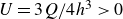 $U=3 Q/4 h^3\gt 0$
; the maximum of the actual inlet and outlet velocities is
$U=3 Q/4 h^3\gt 0$
; the maximum of the actual inlet and outlet velocities is
 $U_{\textit{max}}=3 Q/4 h=Uh^2$
. We have plane Poiseuille flow at infinity of each ‘arm’ (in the far field of the four ends).
$U_{\textit{max}}=3 Q/4 h=Uh^2$
. We have plane Poiseuille flow at infinity of each ‘arm’ (in the far field of the four ends).
(a) Splitting of the whole cross-slot domain into five sub-domains (solid lines indicate real boundaries, dashed lines indicate transition between domain 5 and each of four ‘arms’). (b) Expansions of the Goursat functions
 $f(z)$
and
$f(z)$
and
 $g'(z)$
in each of five sub-domains.
$g'(z)$
in each of five sub-domains.

We decompose our cross-slot domain into five convex polygonal sub-domains, as shown in figure 2(a). Domains 1–4 are unbounded, and domain 5 is bounded, and the arrows show the directions of integration, which will be discussed later.
The flow in each of domains 1, 2 and 5 is symmetric about the
 $x$
-axis (
$x$
-axis (
 $y=0$
), which implies, from the definition of the Schwarz conjugate in (2.9), the symmetry conditions
$y=0$
), which implies, from the definition of the Schwarz conjugate in (2.9), the symmetry conditions
 \begin{equation} \overline {f}(z)=f(z), \quad \overline {g}'(z)=g'(z). \end{equation}
Similarly, the flow in each of domains 3, 4 and 5 is symmetric about the
 $y$
-axis (
$y$
-axis (
 $x=0$
), giving the symmetry conditions
$x=0$
), giving the symmetry conditions
 \begin{equation} \overline {f}(z)=-f(-z), \quad \overline {g}'(z)=-g'(-z). \end{equation}
4. Expansions of the Goursat functions
We expand the Goursat functions of each sub-domain into forcing terms, which capture the far-field behaviour of pressure-driven flow, and correction terms, which will be found through the UTM (Fokas Reference Fokas1997, Reference Fokas2008), as shown in figure 2(b). The details of the decomposition will be discussed later in this section.
4.1. Domain 1
The expansions of the Goursat functions of domain 1 take the form
 \begin{equation} f(z)=f_{s}(z)+f_{1}(z), \quad g'(z)=g'_{s}(z)+g'_{1}(z), \end{equation}
where
 $f_{s} (z )$
and
$f_{s} (z )$
and
 $g'_{s} (z )$
are forcing terms, and
$g'_{s} (z )$
are forcing terms, and
 $f_{1} (z )$
and
$f_{1} (z )$
and
 $g'_{1} (z )$
are correction terms.
$g'_{1} (z )$
are correction terms.
We write the forcing terms
 $f_{s} (z )$
and
$f_{s} (z )$
and
 $g'_{s} (z )$
of domain 1 as
$g'_{s} (z )$
of domain 1 as
 \begin{equation} f_{s}(z)=-\dfrac {U z^{2}}{4} + Pz + c_{\textit{in}}, \quad g'_{s}(z)=\dfrac {U z^{2}}{4} + U h^{2} + c_{\textit{in}}. \end{equation}
Here, we add a linear contribution
 $Pz$
with
$Pz$
with
 $P \in \mathbb{R}$
to domains 1 and 2, and additive parameters
$P \in \mathbb{R}$
to domains 1 and 2, and additive parameters
 $c_{\textit{in}} \in \mathbb{C}$
and
$c_{\textit{in}} \in \mathbb{C}$
and
 $-c_{\textit{in}}$
as constant terms to them, respectively. Without any loss of generality, we do not add any linear term to domains 3 and 4; however, it is still necessary to add complex additive parameters
$-c_{\textit{in}}$
as constant terms to them, respectively. Without any loss of generality, we do not add any linear term to domains 3 and 4; however, it is still necessary to add complex additive parameters
 $c_{\textit{out}}$
and
$c_{\textit{out}}$
and
 $-c_{\textit{out}}$
to them, respectively, as shown below. From the symmetry condition (3.2) we can deduce that
$-c_{\textit{out}}$
to them, respectively, as shown below. From the symmetry condition (3.2) we can deduce that
 $c_{\textit{in}} \in \mathbb{R}$
, and it can also be deduced from (3.3) that
$c_{\textit{in}} \in \mathbb{R}$
, and it can also be deduced from (3.3) that
 $c_{\textit{out}} \in {\mathrm{i}} \mathbb{R}$
. We will see later that
$c_{\textit{out}} \in {\mathrm{i}} \mathbb{R}$
. We will see later that
 $P$
has a connection with the value of the Couette correction, and that there is a relation between the constant parameters
$P$
has a connection with the value of the Couette correction, and that there is a relation between the constant parameters
 $c_{\textit{in}}$
and
$c_{\textit{in}}$
and
 $c_{\textit{out}}$
.
$c_{\textit{out}}$
.
The correction terms
 $f_{1} (z )$
and
$f_{1} (z )$
and
 $g'_{1} (z )$
can then be represented in terms of so-called spectral functions, and can be found through the UTM (Fokas Reference Fokas1997, Reference Fokas2008), as shown below. It is easy to see that the correction terms decay well in the far field so that the integrals make no contribution in the far field, and the Cauchy integral formula can be generalised into unbounded domains. The correction term
$g'_{1} (z )$
can then be represented in terms of so-called spectral functions, and can be found through the UTM (Fokas Reference Fokas1997, Reference Fokas2008), as shown below. It is easy to see that the correction terms decay well in the far field so that the integrals make no contribution in the far field, and the Cauchy integral formula can be generalised into unbounded domains. The correction term
 $f_{1} (z )$
can be represented in terms of spectral functions (Fokas & Kapaev Reference Fokas and Kapaev2003) as
$f_{1} (z )$
can be represented in terms of spectral functions (Fokas & Kapaev Reference Fokas and Kapaev2003) as
 \begin{equation} f_{1}(z)=\dfrac {1}{2 \pi }\left [ \int _{0}^{\infty } { \rho _{1}(k) \mathrm{e}^{{\mathrm{i}} k z}\, {\mathrm{d}} k} + \int _{0}^{-\infty } { \rho _{2}(k) \mathrm{e}^{{\mathrm{i}} k z}\, {\mathrm{d}} k}+\int _{0}^{-{\mathrm{i}} \infty } { \rho _{3}(k) \mathrm{e}^{{\mathrm{i}} k z}\, {\mathrm{d}} k}\right ]\!, \end{equation}
with spectral functions of the form
 \begin{align} \rho _{1}(k)=\int _{-\infty -{\mathrm{i}} h}^{-h-{\mathrm{i}} h} {f_{1}(z) \mathrm{e}^{-{\mathrm{i}} k z}\, {\mathrm{d}} z}, &\quad \rho _{2}(k)=\int _{-h+{\mathrm{i}} h}^{-\infty +{\mathrm{i}} h} {f_{1}(z) \mathrm{e}^{-{\mathrm{i}} k z}\, {\mathrm{d}} z} , \end{align}
 \begin{align} \rho _{3}(k)=\int _{-h-{\mathrm{i}} h}^{-h+{\mathrm{i}} h} &{f_{1}(z) \mathrm{e}^{-{\mathrm{i}} k z}\, {\mathrm{d}} z} . \end{align}
According to Cauchy’s theorem, the spectral functions satisfy the global relation
 \begin{equation} \rho _{1}(k)+\rho _{2}(k)+\rho _{3}(k)=0, \quad \text{Im}\left [k\right ]\geq 0. \end{equation}
Similar to (4.3)–(4.5), the correction term
 $g'_{1} (z )$
can be written in terms of the spectral functions
$g'_{1} (z )$
can be written in terms of the spectral functions
 $\hat {\rho }_{j} (k )$
,
$\hat {\rho }_{j} (k )$
,
 $j=1,2,3$
, with a similar global relation.
$j=1,2,3$
, with a similar global relation.
4.2. Domains 2, 3 and 4
Similar to domain 1, the Goursat functions of domain 2 can be expanded into
 \begin{equation} f(z)=f_{t}(z)+f_{2}(z), \quad g'(z)=g'_{t}(z)+g'_{2}(z), \end{equation}
where the forcing terms
 $f_{t} (z )$
,
$f_{t} (z )$
,
 $g'_{t} (z )$
are given by
$g'_{t} (z )$
are given by
 \begin{equation} f_{t}(z)=\dfrac {U z^{2}}{4} + Pz - c_{\textit{in}}, \quad g'_{t}(z)= - \dfrac {U z^{2}}{4} - U h^{2} - c_{\textit{in}}, \end{equation}
and the correction term
 $f_{2} (z )$
can be represented by
$f_{2} (z )$
can be represented by
 \begin{equation} f_{2}(z)=\dfrac {1}{2 \pi }\left [ \int _{0}^{\infty } { \sigma _{1}(k) \mathrm{e}^{{\mathrm{i}} k z}\, {\mathrm{d}} k} + \int _{0}^{-\infty } { \sigma _{2}(k) \mathrm{e}^{{\mathrm{i}} k z}\, {\mathrm{d}} k} + \int _{0}^{{\mathrm{i}} \infty } { \sigma _{3}(k) \mathrm{e}^{{\mathrm{i}} k z}\, {\mathrm{d}} k} \right ]\!, \end{equation}
with the spectral functions
 \begin{align} \sigma _{1}(k)=\int _{h-{\mathrm{i}} h}^{\infty -{\mathrm{i}} h} {f_{2}(z) \mathrm{e}^{-{\mathrm{i}} k z}\, {\mathrm{d}} z}, &\quad \sigma _{2}(k)=\int _{\infty +{\mathrm{i}} h}^{h+{\mathrm{i}} h} {f_{2}(z) \mathrm{e}^{-{\mathrm{i}} k z}\, {\mathrm{d}} z} , \end{align}
 \begin{align} \sigma _{3}(k)=\int _{h+{\mathrm{i}} h}^{h-{\mathrm{i}} h} &{f_{2}(z) \mathrm{e}^{-{\mathrm{i}} k z}\, {\mathrm{d}} z} . \end{align}
The spectral functions satisfy the global relation
 \begin{equation} \sigma _{1}(k)+\sigma _{2}(k)+\sigma _{3}(k)=0, \quad \text{Im}\left [k\right ]\leq 0. \end{equation}
Expressions similar to (4.8)–(4.10) can be written for
 $g'_{2} (z )$
(in terms of
$g'_{2} (z )$
(in terms of
 $\hat {\sigma }_{j} (k )$
,
$\hat {\sigma }_{j} (k )$
,
 $j=1,2,3$
).
$j=1,2,3$
).
The expansions of the Goursat functions of domain 3 take the form
 \begin{equation} f(z)=f_{u}(z)+f_{3}(z), \quad g'(z)=g'_{u}(z)+g'_{3}(z), \end{equation}
with forcing terms
 \begin{equation} f_{u}(z)=\dfrac {{\mathrm{i}} U z^{2}}{4} + c_{\textit{out}}, \quad g'_{u}(z)=\dfrac {{\mathrm{i}} U z^{2}}{4} - {\mathrm{i}} U h^{2} - c_{\textit{out}}, \end{equation}
and the correction term
 $f_{3} (z )$
can be written as
$f_{3} (z )$
can be written as
 \begin{equation} f_{3}(z)=\dfrac {1}{2 \pi }\left [ \int _{0}^{- {\mathrm{i}} \infty } { \tau _{1}(k) \mathrm{e}^{{\mathrm{i}} k z} \,{\mathrm{d}} k} + \int _{0}^{{\mathrm{i}} \infty } { \tau _{2}(k) \mathrm{e}^{{\mathrm{i}} k z}\, {\mathrm{d}} k} + \int _{0}^{\infty } { \tau _{3}(k) \mathrm{e}^{{\mathrm{i}} k z}\, {\mathrm{d}} k} \right ]\!, \end{equation}
using the spectral functions
 \begin{align} \tau _{1}(k)=\int _{h+{\mathrm{i}} h}^{h+{\mathrm{i}} \infty } {f_{3}(z) \mathrm{e}^{-{\mathrm{i}} k z}\, {\mathrm{d}} z}, &\quad \tau _{2}(k)=\int _{-h+{\mathrm{i}} \infty }^{-h+{\mathrm{i}} h} {f_{3}(z) \mathrm{e}^{-{\mathrm{i}} k z}\, {\mathrm{d}} z} , \end{align}
 \begin{align} \tau _{3}(k)=\int _{-h+{\mathrm{i}} h}^{h+{\mathrm{i}} h} &{f_{3}(z) \mathrm{e}^{-{\mathrm{i}} k z}\, {\mathrm{d}} z} , \end{align}
and the global relation becomes
 \begin{equation} \tau _{1}(k)+\tau _{2}(k)+\tau _{3}(k)=0, \quad \text{Re}\left [k\right ]\leq 0. \end{equation}
Similar to (4.13)–(4.15),
 $g'_{3} (z )$
can be written in terms of
$g'_{3} (z )$
can be written in terms of
 $\hat {\tau }_{j} (k )$
,
$\hat {\tau }_{j} (k )$
,
 $j=1,2,3$
, with a similar global relation.
$j=1,2,3$
, with a similar global relation.
Similarly, for the Goursat functions of domain 4, we write
 \begin{equation} f(z)=f_{v}(z)+f_{4}(z), \quad g'(z)=g'_{v}(z)+g'_{4}(z), \end{equation}
with forcing terms
 \begin{equation} f_{v}(z)= - \dfrac {{\mathrm{i}} U z^{2}}{4} - c_{\textit{out}}, \quad g'_{v}(z)= - \dfrac {{\mathrm{i}} U z^{2}}{4} + {\mathrm{i}} U h^{2} + c_{\textit{out}}, \end{equation}
and the representation of the correction term as
 \begin{equation} f_{4}(z)=\dfrac {1}{2 \pi }\left [ \int _{0}^{- {\mathrm{i}} \infty } { \chi _{1}(k) \mathrm{e}^{{\mathrm{i}} k z} \,{\mathrm{d}} k} + \int _{0}^{{\mathrm{i}} \infty } { \chi _{2}(k) \mathrm{e}^{{\mathrm{i}} k z}\, {\mathrm{d}} k} + \int _{0}^{- \infty } { \chi _{3}(k) \mathrm{e}^{{\mathrm{i}} k z}\, {\mathrm{d}} k} \right ]\!, \end{equation}
using spectral functions
 \begin{align} \chi _{1}(k)=\int _{h-{\mathrm{i}}\infty }^{h-{\mathrm{i}} h} {f_{4}(z) \mathrm{e}^{-{\mathrm{i}} k z}\, {\mathrm{d}} z}, &\quad \chi _{2}(k)=\int _{-h-{\mathrm{i}} h}^{-h-{\mathrm{i}}\infty } {f_{4}(z) \mathrm{e}^{-{\mathrm{i}} k z}\, {\mathrm{d}} z} , \end{align}
 \begin{align} \chi _{3}(k)=\int _{h-{\mathrm{i}} h}^{-h-{\mathrm{i}} h} &{f_{4}(z) \mathrm{e}^{-{\mathrm{i}} k z}\, {\mathrm{d}} z} . \end{align}
The global relation becomes
 \begin{equation} \chi _{1}(k)+\chi _{2}(k)+\chi _{3}(k)=0, \quad \text{Re}\left [k\right ]\geq 0. \end{equation}
We can write expressions similar to (4.18)–(4.20) for
 $g'_{4} (z )$
in terms of
$g'_{4} (z )$
in terms of
 $\hat {\chi }_{j} (k )$
,
$\hat {\chi }_{j} (k )$
,
 $j=1,2,3$
.
$j=1,2,3$
.
4.3. Domain 5
Since domain 5 is a bounded sub-domain, the Goursat functions in domain 5 have correction terms only. Hence we have
 \begin{equation} f(z)=f_{5}(z), \quad g'(z)=g'_{5}(z). \end{equation}
Similarly, the correction term
 $f_{5} (z )$
can also be written in terms of spectral functions:
$f_{5} (z )$
can also be written in terms of spectral functions:
 \begin{eqnarray} f_{5}(z)&=&\dfrac {1}{2 \pi }\left [ \int _{0}^{\infty } { \upsilon _{1}(k) \mathrm{e}^{{\mathrm{i}} k z} \,{\mathrm{d}} k} + \int _{0}^{-{\mathrm{i}} \infty } { \upsilon _{2}(k) \mathrm{e}^{{\mathrm{i}} k z}\, {\mathrm{d}} k} \right . \nonumber \\ && \quad \left . {}+ \int _{0}^{- \infty } { \upsilon _{3}(k) \mathrm{e}^{{\mathrm{i}} k z}\, {\mathrm{d}} k} + \int _{0}^{{\mathrm{i}} \infty } { \upsilon _{4}(k) \mathrm{e}^{{\mathrm{i}} k z}\, {\mathrm{d}} k} \right ]\!, \end{eqnarray}
where the spectral functions are
 \begin{align} \upsilon _{1}(k)=\int _{-h-{\mathrm{i}} h}^{h-{\mathrm{i}} h} {f_{5}(z) \mathrm{e}^{-{\mathrm{i}} k z}\, {\mathrm{d}} z}, &\quad \upsilon _{2}(k)=\int _{h-{\mathrm{i}} h}^{h+{\mathrm{i}} h} {f_{5}(z) \mathrm{e}^{-{\mathrm{i}} k z}\, {\mathrm{d}} z} , \end{align}
 \begin{align} \upsilon _{3}(k)=\int _{h+{\mathrm{i}} h}^{-h+{\mathrm{i}} h} {f_{5}(z) \mathrm{e}^{-{\mathrm{i}} k z}\, {\mathrm{d}} z}, &\quad \upsilon _{4}(k)=\int _{-h+{\mathrm{i}} h}^{-h-{\mathrm{i}} h} {f_{5}(z) \mathrm{e}^{-{\mathrm{i}} k z}\, {\mathrm{d}} z} , \end{align}
and the global relation is
 \begin{equation} \upsilon _{1}(k)+\upsilon _{2}(k)+\upsilon _{3}(k)+\upsilon _{4}(k)=0, \quad k \in \mathbb{C}. \end{equation}
Similar to (4.22)–(4.24), the correction term
 $g'_{5} (z )$
can be written in terms of the spectral functions
$g'_{5} (z )$
can be written in terms of the spectral functions
 $\hat {\upsilon }_{j} (k )$
,
$\hat {\upsilon }_{j} (k )$
,
 $j=1,2,3,4$
, with a similar global relation.
$j=1,2,3,4$
, with a similar global relation.
5. Spectral analysis
In this section, we will use the no-slip boundary condition (3.1) on the channel walls to obtain relations between the spectral functions.
5.1. Domain 1
Using the symmetry condition in (3.2) and the expansions (4.1), on the lower boundary
 ${\overline {z}}=z+2{\mathrm{i}} h$
we have
${\overline {z}}=z+2{\mathrm{i}} h$
we have
 \begin{equation} -f_{1}\left (z+2{\mathrm{i}} h\right )+\left (z+2{\mathrm{i}} h\right ) f'_{1}(z)+g'_{1}(z)=0. \end{equation}
Similarly, on the upper boundary
 ${\overline {z}}=z-2{\mathrm{i}} h$
we have
${\overline {z}}=z-2{\mathrm{i}} h$
we have
 \begin{equation} -f_{1}\left (z-2{\mathrm{i}} h\right )+\left (z-2{\mathrm{i}} h\right ) f'_{1}(z)+g'_{1}(z)=0. \end{equation}
Multiplying (5.1) by
 $\mathrm{e}^{-{\mathrm{i}} kz}$
and integrating along the lower boundary (in the arrow direction shown in figure 2), it can be shown that
$\mathrm{e}^{-{\mathrm{i}} kz}$
and integrating along the lower boundary (in the arrow direction shown in figure 2), it can be shown that
 \begin{align} \mathrm{e}^{-2kh}\, \rho _{2}(k)-\dfrac {\partial \left [k \rho _{1}(k)\right ]}{\partial k}-2kh\, \rho _{1}(k)+\hat {\rho }_{1}(k) + \left (-h+{\mathrm{i}} h\right ) f_{1}\left (-h-{\mathrm{i}} h\right ) \mathrm{e}^{-{\mathrm{i}} k \left (-h-{\mathrm{i}} h\right )}=0.\\[-20pt]\nonumber \end{align}
Similarly, multiplying (5.2) by
 $\mathrm{e}^{-{\mathrm{i}} kz}$
and integrating along the upper boundary (in the arrow direction shown in figure 2), we can show that
$\mathrm{e}^{-{\mathrm{i}} kz}$
and integrating along the upper boundary (in the arrow direction shown in figure 2), we can show that
 \begin{equation} \mathrm{e}^{2kh}\, \rho _{1}(k)-\dfrac {\partial \left [k \rho _{2}(k)\right ]}{\partial k}+2kh\, \rho _{2}(k)+\hat {\rho }_{2}(k) - \left (-h-{\mathrm{i}} h\right ) f_{1}\left (-h+{\mathrm{i}} h\right ) \mathrm{e}^{-{\mathrm{i}} k\left (-h+{\mathrm{i}} h\right )}=0. \end{equation}
Adding (5.3) and (5.4), and using the global relation (4.5), we have
 \begin{equation} 2\left [\sinh \left (2kh\right )-2kh\right ] \rho _{1}(k)=W_{1}(k), \quad \text{Im}\left [k\right ]\geq 0, \end{equation}
where
 \begin{eqnarray} W_{1}(k)&=&\big [\mathrm{e}^{-2kh}+2kh\big ] \rho _{3}(k) - \dfrac {\partial \left [k\, \rho _{3}(k)\right ]}{\partial k}+\hat {\rho }_{3}(k) \nonumber \\ && \mbox{} -\left (-h+{\mathrm{i}} h\right ) f_{1}\left (-h-{\mathrm{i}} h\right ) \mathrm{e}^{-{\mathrm{i}} k \left (-h-{\mathrm{i}} h\right )} \nonumber \\ && \mbox{} +\left (-h-{\mathrm{i}} h\right ) f_{1}\left (-h+{\mathrm{i}} h\right ) \mathrm{e}^{-{\mathrm{i}} k\left (-h+{\mathrm{i}} h\right )}. \end{eqnarray}
5.2. Domains 2, 3 and 4
Using similar spectral analysis and the global relations (4.10), (4.15) and (4.20), respectively, we can deduce that
 \begin{equation} 2\left [\sinh \left (2kh\right )-2kh\right ] \sigma _{1}(k)=W_{2}(k), \quad \text{Im}\left [k\right ]\leq 0, \end{equation}
where
 \begin{eqnarray} W_{2}(k)&=&\big [\mathrm{e}^{-2kh}+2kh\big ] \sigma _{3}(k) - \dfrac {\partial \left [k\, \sigma _{3}(k)\right ]}{\partial k}+\hat {\sigma }_{3}(k) \nonumber \\ && \mbox{} +\left (h+{\mathrm{i}} h\right ) f_{2}\left (h-{\mathrm{i}} h\right ) \mathrm{e}^{-{\mathrm{i}} k\left (h-{\mathrm{i}} h\right )} \nonumber \\ && \mbox{} -\left (h-{\mathrm{i}} h\right ) f_{2}\left (h+{\mathrm{i}} h\right ) \mathrm{e}^{-{\mathrm{i}} k\left (h+{\mathrm{i}} h\right )}, \end{eqnarray}
and that
 \begin{equation} 2\big [\sinh \left (2{\mathrm{i}} kh\right )-2{\mathrm{i}} kh\big ] \tau _{1}(k)=W_{3}(k), \quad \text{Re}\left [k\right ]\leq 0, \end{equation}
where
 \begin{eqnarray} W_{3}(k)&=&\big [\mathrm{e}^{-2{\mathrm{i}} kh}+2{\mathrm{i}} kh\big ] \tau _{3}(k) - \dfrac {\partial \left [k\, \tau _{3}(k)\right ]}{\partial k}-\hat {\tau }_{3}(k) \nonumber \\ && \mbox{} +\left (-h+{\mathrm{i}} h\right ) f_{3}\left (h+{\mathrm{i}} h\right ) \mathrm{e}^{-{\mathrm{i}} k\left (h+{\mathrm{i}} h\right )} \nonumber \\ && \mbox{} -\left (h+{\mathrm{i}} h\right ) f_{3}\left (-h+{\mathrm{i}} h\right ) \mathrm{e}^{-{\mathrm{i}} k\left (-h+{\mathrm{i}} h\right )}, \end{eqnarray}
and finally that
 \begin{equation} 2\left [\sinh \left (2{\mathrm{i}} kh\right )-2{\mathrm{i}} kh\right ] \chi _{1}(k)=W_{4}(k), \quad \text{Re}\left [k\right ]\geq 0, \end{equation}
where
 \begin{eqnarray} W_{4}(k)&=&\big [\mathrm{e}^{-2{\mathrm{i}} kh}+2{\mathrm{i}} kh\big ] \chi _{3}(k) - \dfrac {\partial \left [k\, \chi _{3}(k)\right ]}{\partial k}-\hat {\chi }_{3}(k) \nonumber \\ && \mbox{} -\left (-h-{\mathrm{i}} h\right ) f_{4}\left (h-{\mathrm{i}} h\right ) \mathrm{e}^{-{\mathrm{i}} k\left (h-{\mathrm{i}} h\right )} \nonumber \\ && \mbox{} +\left (h-{\mathrm{i}} h\right ) f_{4}\left (-h-{\mathrm{i}} h\right ) \mathrm{e}^{-{\mathrm{i}} k\left (-h-{\mathrm{i}} h\right )}. \end{eqnarray}
More mathematical details of the spectral analysis of these sub-domains are given in Appendix A.
6. Continuity conditions
Imposing the continuity of velocity, pressure and vorticity along the transition between neighbouring sub-domains, we can obtain continuity conditions for the Goursat functions.
For the transition between domains 1 and 5, along
 $z=-h+{\mathrm{i}} y$
,
$z=-h+{\mathrm{i}} y$
,
 $y \in [-h,h ]$
, we have
$y \in [-h,h ]$
, we have
 \begin{equation} f_{s}(z)+f_{1}(z)=f_{5}(z), \quad g'_{s}(z)+g'_{1}(z)=g'_{5}(z). \end{equation}
Similarly, between domains 2 and 5, along
 $z=h+{\mathrm{i}} y$
,
$z=h+{\mathrm{i}} y$
,
 $y \in [-h,h]$
, we have
$y \in [-h,h]$
, we have
 \begin{equation} f_{5}(z)=f_{t}(z)+f_{2}(z), \quad g'_{5}(z)=g'_{t}(z)+g'_{2}(z); \end{equation}
between domains 3 and 5, along
 $z=x+{\mathrm{i}} h$
,
$z=x+{\mathrm{i}} h$
,
 $x \in [-h,h ]$
, we have
$x \in [-h,h ]$
, we have
 \begin{equation} f_{u}(z)+f_{3}(z)=f_{5}(z), \quad g'_{u}(z)+g'_{3}(z)=g'_{5}(z); \end{equation}
and finally between domains 4 and 5, along
 $z=x-{\mathrm{i}} h$
,
$z=x-{\mathrm{i}} h$
,
 $x \in [-h,h]$
, we have
$x \in [-h,h]$
, we have
 \begin{equation} f_{5}(z)=f_{v}(z)+f_{4}(z), \quad g'_{5}(z)=g'_{v}(z)+g'_{4}(z). \end{equation}
7. Solution scheme
In this section, we formulate the linear system to calculate the Goursat functions along the transition between domain 5 and each of the four ‘arms’. We will discuss three different possibilities: without the use of any symmetry condition, with the use of a symmetry condition in domain 5 only, and finally with the use of a symmetry condition in domain 5 and symmetry between each pair of opposite ‘arms’. We will compare the results under these different conditions to ensure computational accuracy of our results, and investigate whether our transform approach can capture the symmetry conditions ‘automatically’, and whether this method can be used to solve Stokes flow problems in further complicated geometries.
After spectral analysis, we have the following system:
 \begin{align} &2\left [\sinh \left (2kh\right )-2kh\right ] \rho _{1}(k)=W_{1}(k), \quad\,\, \text{Im}\left [k\right ]\geq 0, \end{align}
 \begin{align} &2\left [\sinh \left (2kh\right )-2kh\right ] \sigma _{1}(k)=W_{2}(k), \quad\,\, \text{Im}\left [k\right ]\leq 0, \end{align}
 \begin{align} &2\left [\sinh \left (2{\mathrm{i}} kh\right )-2{\mathrm{i}} kh\right ] \tau _{1}(k)=W_{3}(k), \quad \text{Re}\left [k\right ]\leq 0, \end{align}
 \begin{align} &2\left [\sinh \left (2{\mathrm{i}} kh\right )-2{\mathrm{i}} kh\right ] \chi _{1}(k)=W_{4}(k), \quad\! \text{Re}\left [k\right ]\geq 0. \end{align}
Here, since the spectral functions
 $\rho _{1} (k )$
,
$\rho _{1} (k )$
,
 $\sigma _{1} (k )$
,
$\sigma _{1} (k )$
,
 $\tau _{1} (k )$
and
$\tau _{1} (k )$
and
 $\chi _{1} (k )$
are analytic in their corresponding spectral
$\chi _{1} (k )$
are analytic in their corresponding spectral
 $k$
-plane (half-plane), respectively, we have
$k$
-plane (half-plane), respectively, we have
 \begin{align} &W_{1}(k)=0 \quad \mbox{for } \ k \in \varSigma _{1} \equiv \{k: \text{Im}\left [k\right ] \geq 0\, | \sinh \left (2kh\right )-2kh=0\}, \end{align}
 \begin{align} &W_{2}(k)=0 \quad \mbox{for } \ k \in \varSigma _{2} \equiv \{k: \text{Im}\left [k\right ] \leq 0\, | \sinh \left (2kh\right )-2kh=0\}, \end{align}
 \begin{align} &W_{3}(k)=0 \quad \mbox{for } \ k \in \varSigma _{3} \equiv \{k: \text{Re}\left [k\right ] \leq 0\, | \sinh \left (2{\mathrm{i}} kh\right )-2{\mathrm{i}} kh=0\}, \end{align}
 \begin{align} &W_{4}(k)=0 \quad \mbox{for } \ k \in \varSigma _{4} \equiv \{k: \text{Re}\left [k\right ] \geq 0\, | \sinh \left (2{\mathrm{i}} kh\right )-2{\mathrm{i}} kh=0\}. \end{align}
We also have
 \begin{equation} \sinh \left (2kh\right )-2kh=O\big (k^3\big ) \quad \mbox{as } \ k \rightarrow 0, \end{equation}
which indicates that
 \begin{align} W_{1}\left (0\right )=W_{1}'\left (0\right )=W_{1}''\left (0\right )=0, \end{align}
 \begin{align} W_{2}\left (0\right )=W_{2}'\left (0\right )=W_{2}''\left (0\right )=0,\end{align}
 \begin{align} W_{3}\left (0\right )=W_{3}'\left (0\right )=W_{3}''\left (0\right )=0, \end{align}
 \begin{align} W_{4}\left (0\right )=W_{4}'\left (0\right )=W_{4}''\left (0\right )=0. \end{align}
We have now reduced our problem to that of determining the values of
 $f (z )$
and
$f (z )$
and
 $g' (z )$
along the transition between neighbouring sub-domains, i.e. along the four edges of domain 5. We now expand each of these in terms of Chebyshev polynomials:
$g' (z )$
along the transition between neighbouring sub-domains, i.e. along the four edges of domain 5. We now expand each of these in terms of Chebyshev polynomials:
 \begin{align} f_5\left (z_{1}\left (s\right )\right )&=\sum _{m=0}^{\infty } {a_{m}\, T_{m}\left (s\right )}, \quad g'_5\left (z_{1}\left (s\right )\right )=\sum _{m=0}^{\infty } {A_{m}\, T_{m}\left (s\right )}, \end{align}
 \begin{align} f_5\left (z_{2}\left (s\right )\right )&=\sum _{m=0}^{\infty } {b_{m}\, T_{m}\left (s\right )}, \quad g'_5\left (z_{2}\left (s\right )\right )=\sum _{m=0}^{\infty } {B_{m}\, T_{m}\left (s\right )}, \end{align}
 \begin{align} f_5\left (z_{3}\left (s\right )\right )&=\sum _{m=0}^{\infty } {c_{m}\, T_{m}\left (s\right )}, \quad g'_5\left (z_{3}\left (s\right )\right )=\sum _{m=0}^{\infty } {C_{m}\, T_{m}\left (s\right )}, \end{align}
 \begin{align} f_5\left (z_{4}\left (s\right )\right )&=\sum _{m=0}^{\infty } {d_{m}\, T_{m}\left (s\right )}, \quad g'_5\left (z_{4}\left (s\right )\right )=\sum _{m=0}^{\infty } {D_{m}\, T_{m}\left (s\right )}, \end{align}
where the four edges of domain 5 are parametrised in the obvious way in terms of a new variable
 $s$
:
$s$
:
 \begin{align} z_1\left (s\right )&=hs-{\mathrm{i}} h, \quad\,\,\,\, s \in \left [-1,1\right ], \end{align}
 \begin{align} z_2\left (s\right )&=h+{\mathrm{i}} h s, \quad\,\,\,\, s \in \left [-1,1\right ], \end{align}
 \begin{align} z_3\left (s\right )&=-hs+{\mathrm{i}} h, \quad s \in \left [-1,1\right ], \end{align}
 \begin{align} z_4\left (s\right )&=-h-{\mathrm{i}} h s, \quad s \in \left [-1,1\right ]. \end{align}
Here,
 $T_{m} (s )=\cos (m \cos ^{-1} (s ) )$
is the
$T_{m} (s )=\cos (m \cos ^{-1} (s ) )$
is the
 $m$
th Chebyshev polynomial of the first kind (Boyd Reference Boyd2000), and
$m$
th Chebyshev polynomial of the first kind (Boyd Reference Boyd2000), and
 $\{a_{m}, b_{m}, c_{m}, d_{m}, A_{m}, B_{m}, C_{m}, D_{m}\}$
are the unknown coefficients that need to be calculated. According to (4.23), the spectral functions of domain 5 can then be expressed as
$\{a_{m}, b_{m}, c_{m}, d_{m}, A_{m}, B_{m}, C_{m}, D_{m}\}$
are the unknown coefficients that need to be calculated. According to (4.23), the spectral functions of domain 5 can then be expressed as
 \begin{align} \upsilon _{1}(k)&=\sum _{m=0}^{\infty } {a_{m} \left [T_1\left (k,m\right )\right ]}, \quad \hat {\upsilon }_{1}(k)=\sum _{m=0}^{\infty } {A_{m} \left [T_1\left (k,m\right )\right ]}, \end{align}
 \begin{align} \upsilon _{2}(k)&=\sum _{m=0}^{\infty } {b_{m} \left [T_2\left (k,m\right )\right ]}, \quad \hat {\upsilon }_{2}(k)=\sum _{m=0}^{\infty } {B_{m} \left [T_2\left (k,m\right )\right ]}, \end{align}
 \begin{align} \upsilon _{3}(k)&=\sum _{m=0}^{\infty } {c_{m} \left [T_3\left (k,m\right )\right ]}, \quad \hat {\upsilon }_{3}(k)=\sum _{m=0}^{\infty } {C_{m} \left [T_3\left (k,m\right )\right ]}, \end{align}
 \begin{align} \upsilon _{4}(k)&=\sum _{m=0}^{\infty } {d_{m} \left [T_4\left (k,m\right )\right ]}, \quad \hat {\upsilon }_{4}(k)=\sum _{m=0}^{\infty } {D_{m} \left [T_4\left (k,m\right )\right ]}, \end{align}
where
 \begin{equation} T_{j}\left (k,m\right )=\int _{-1}^{1} {T_m\left (s\right ) \mathrm{e}^{-{\mathrm{i}} k z_j(s)}\, z'_{j}\left (s\right ) {\mathrm{d}} s}, \quad j=1,2,3,4. \end{equation}
Using the continuity conditions (6.1)–(6.4), we can deduce that
 \begin{align} \chi _{3}(k)&=-\upsilon _{1}(k)+I_{1}(k), \quad \hat {\chi }_{3}(k)=-\hat {\upsilon }_{1}(k)+\hat {I}_{1}(k), \end{align}
 \begin{align} \sigma _{3}(k)&=-\upsilon _{2}(k)+I_{2}(k), \quad \hat {\sigma }_{3}(k)=-\hat {\upsilon }_{2}(k)+\hat {I}_{2}(k), \end{align}
 \begin{align} \tau _{3}(k)&=-\upsilon _{3}(k)+I_{3}(k), \quad \hat {\tau }_{3}(k)=-\hat {\upsilon }_{3}(k)+\hat {I}_{3}(k), \end{align}
 \begin{align} \rho _{3}(k)&=-\upsilon _{4}(k)+I_{4}(k), \quad \hat {\rho }_{3}(k)=-\hat {\upsilon }_{4}(k)+\hat {I}_{4}(k), \end{align}
where
 \begin{align} I_{1}(k)&=\int _{-h-{\mathrm{i}} h}^{h -{\mathrm{i}} h} {f_v(z) \mathrm{e}^{-{\mathrm{i}} k z}\, {\mathrm{d}} z}, \quad\,\, \hat {I}_{1}(k)=\int _{-h-{\mathrm{i}} h}^{h -{\mathrm{i}} h} {g'_v(z) \mathrm{e}^{-{\mathrm{i}} k z}\, {\mathrm{d}} z}, \end{align}
 \begin{align} I_{2}(k)&=\int _{h-{\mathrm{i}} h}^{h +{\mathrm{i}} h} {f_t(z) \mathrm{e}^{-{\mathrm{i}} k z}\, {\mathrm{d}} z}, \quad\,\,\, \hat {I}_{2}(k)=\int _{h-{\mathrm{i}} h}^{h +{\mathrm{i}} h} {g'_t(z) \mathrm{e}^{-{\mathrm{i}} k z}\, {\mathrm{d}} z}, \end{align}
 \begin{align} I_{3}(k)&=\int _{h+{\mathrm{i}} h}^{-h +{\mathrm{i}} h} {f_u(z) \mathrm{e}^{-{\mathrm{i}} k z}\, {\mathrm{d}} z}, \quad \hat {I}_{3}(k)=\int _{h+{\mathrm{i}} h}^{-h +{\mathrm{i}} h} {g'_u(z) \mathrm{e}^{-{\mathrm{i}} k z}\, {\mathrm{d}} z}, \end{align}
 \begin{align} I_{4}(k)&=\int _{-h+{\mathrm{i}} h}^{-h -{\mathrm{i}} h} {f_s(z) \mathrm{e}^{-{\mathrm{i}} k z}\, {\mathrm{d}} z}, \quad \hat {I}_{4}(k)=\int _{-h+{\mathrm{i}} h}^{-h -{\mathrm{i}} h} {g'_s(z) \mathrm{e}^{-{\mathrm{i}} k z}\, {\mathrm{d}} z}. \end{align}
7.1. Without the use of any symmetry condition
Using the continuity conditions (6.1)–(6.4), a linear system can be formulated with conditions in (4.24), (7.2) and (7.4), which allows us to calculate the unknown coefficients
 $\{a_{m}, b_{m}, c_{m}, d_{m}, A_{m}, B_{m}, C_{m}, D_{m}\}$
and the additive parameters
$\{a_{m}, b_{m}, c_{m}, d_{m}, A_{m}, B_{m}, C_{m}, D_{m}\}$
and the additive parameters
 $P$
,
$P$
,
 $c_{\textit{in}}$
and
$c_{\textit{in}}$
and
 $c_{\textit{out}}$
. In order to calculate these unknown coefficients and additive parameters, the infinite series expansions in (7.5) and (7.7) are truncated at suitable
$c_{\textit{out}}$
. In order to calculate these unknown coefficients and additive parameters, the infinite series expansions in (7.5) and (7.7) are truncated at suitable
 $M$
. For moderate values of
$M$
. For moderate values of
 $M$
, we find that the coefficients
$M$
, we find that the coefficients
 $\{a_{m}, b_{m}, c_{m}, d_{m}, A_{m}, B_{m}, C_{m}, D_{m}\}$
that we solve for decay reliably. However, if we truncate at too high a value of
$\{a_{m}, b_{m}, c_{m}, d_{m}, A_{m}, B_{m}, C_{m}, D_{m}\}$
that we solve for decay reliably. However, if we truncate at too high a value of
 $M$
, then we encounter difficulties with convergence: all physical quantities (stress and velocity components) show unphysical artefacts on the transition between neighbouring sub-domains. For this reason, we choose the truncation parameter to be
$M$
, then we encounter difficulties with convergence: all physical quantities (stress and velocity components) show unphysical artefacts on the transition between neighbouring sub-domains. For this reason, we choose the truncation parameter to be
 $M = 8$
, for which the ratios
$M = 8$
, for which the ratios
 $a_8/a_1$
,
$a_8/a_1$
,
 $A_8/A_1$
, and so on are all of order at most
$A_8/A_1$
, and so on are all of order at most
 $10^{-2}$
. Our choice here, using a Chebyshev basis to expand the Goursat functions along the four sides of domain 5, as shown in (7.5), yields convergent solutions with good accuracy in the domain interior. The system size, for
$10^{-2}$
. Our choice here, using a Chebyshev basis to expand the Goursat functions along the four sides of domain 5, as shown in (7.5), yields convergent solutions with good accuracy in the domain interior. The system size, for
 $M=8$
and
$M=8$
and
 $20$
non-zero roots in each spectral
$20$
non-zero roots in each spectral
 $k$
-plane, is
$k$
-plane, is
 $254 \times 75$
. Solving this linear system takes a computational time of less than a second on a standard laptop.
$254 \times 75$
. Solving this linear system takes a computational time of less than a second on a standard laptop.
The presence of sharp corners suggests that instead of Chebyshev expansions, one could employ tailor-made basis functions that account for the precise singularity at each corner. Such an approach was applied by Crowdy & Luca (Reference Crowdy and Luca2014), who used the UTM to analyse a biharmonic mixed boundary value problem; they introduced a uniformisation variable incorporating the known singular behaviour near corner points, and used it in a polynomial expansion to represent the unknown data. It was shown that spectrally accurate results were obtained. More recently, Colbrook and co-workers (Colbrook, Flyer & Fornberg Reference Colbrook, Flyer and Fornberg2018, Reference Colbrook, Ayton and Fokas2019a ,Reference Colbrook, Ayton and Fokas b ; Colbrook Reference Colbrook2020) proposed methods for addressing elliptic problems (for Laplace’s, modified Helmholtz and Helmholtz equations) via the UTM in domains with corner singularities, which embed the known corner behaviour directly into the approximation scheme. While these strategies are relevant in the present context for the biharmonic equation, their implementation lies beyond the scope of this study. The use of a Chebyshev basis nevertheless provides good accuracy both in the domain interior and in the vicinity of the corners.
7.2. With the use of a symmetry condition in domain 5 only
If we use a symmetry condition in domain 5, then the global relation of domain 5 takes the form
 \begin{align} \upsilon _{1}(k)+\upsilon _{2}(k)+\upsilon _{1}\left (-k\right )+\upsilon _{2}\left (-k\right )=0, & \quad k \in \mathbb{C}, \end{align}
 \begin{align} \hat {\upsilon }_{1}(k)+\hat {\upsilon }_{2}(k)+\hat {\upsilon }_{1}\left (-k\right )+\hat {\upsilon }_{2}\left (-k\right )=0, & \quad k \in \mathbb{C}, \end{align}
 \begin{align} \upsilon _{3}(k)+\upsilon _{4}(k)+\upsilon _{3}\left (-k\right )+\upsilon _{4}\left (-k\right )=0, & \quad k \in \mathbb{C}, \end{align}
 \begin{align} \hat {\upsilon }_{3}(k)+\hat {\upsilon }_{4}(k)+\hat {\upsilon }_{3}\left (-k\right )+\hat {\upsilon }_{4}\left (-k\right )=0, & \quad k \in \mathbb{C}. \end{align}
The system of equations in (7.2), (7.4) and (7.11) allows us to calculate the unknown coefficients
 $\{a_{m}, b_{m}, c_{m}, d_{m}, A_{m}, B_{m}, C_{m}, D_{m}\,|\, m=0,\ldots ,M\}$
and the additive parameters
$\{a_{m}, b_{m}, c_{m}, d_{m}, A_{m}, B_{m}, C_{m}, D_{m}\,|\, m=0,\ldots ,M\}$
and the additive parameters
 $P$
,
$P$
,
 $c_{\textit{in}}$
and
$c_{\textit{in}}$
and
 $c_{\textit{out}}$
.
$c_{\textit{out}}$
.
7.3. With the use of a symmetry condition in domain 5 and symmetry between each pair of opposite ‘arms’
If we use the symmetry between domains 1 and 2, and the symmetry between domains 3 and 4, then the system of equations in (7.2) and (7.4), and the last two equations in (7.11), allow us to calculate the unknown coefficients
 $\{c_{m}, d_{m}, C_{m}, D_{m}\,|\, m=0,\ldots ,M\}$
and the additive parameters
$\{c_{m}, d_{m}, C_{m}, D_{m}\,|\, m=0,\ldots ,M\}$
and the additive parameters
 $P$
,
$P$
,
 $c_{\textit{in}}$
and
$c_{\textit{in}}$
and
 $c_{\textit{out}}$
.
$c_{\textit{out}}$
.
More mathematical details of the analysis using these symmetry conditions are given in Appendix B.
The coefficients
 $\{a_{m}, b_{m}, c_{m}, d_{m}, A_{m}, B_{m}, C_{m}, D_{m}\,|\, m=0,\ldots ,M\}$
(with some or no symmetry conditions) or
$\{a_{m}, b_{m}, c_{m}, d_{m}, A_{m}, B_{m}, C_{m}, D_{m}\,|\, m=0,\ldots ,M\}$
(with some or no symmetry conditions) or
 $\{c_{m}, d_{m}, C_{m}, D_{m}\,|\, m=0,\ldots ,M\}$
(with all symmetry conditions) and the additive parameters
$\{c_{m}, d_{m}, C_{m}, D_{m}\,|\, m=0,\ldots ,M\}$
(with all symmetry conditions) and the additive parameters
 $P$
,
$P$
,
 $c_{\textit{in}}$
and
$c_{\textit{in}}$
and
 $c_{\textit{out}}$
have been computed; the results can be obtained within only a second on a standard laptop for
$c_{\textit{out}}$
have been computed; the results can be obtained within only a second on a standard laptop for
 $M=8$
, and it has been confirmed that the result is stable in terms of both the number of roots in the spectral
$M=8$
, and it has been confirmed that the result is stable in terms of both the number of roots in the spectral
 $k$
-planes and the truncation of Chebyshev expansions (choice of
$k$
-planes and the truncation of Chebyshev expansions (choice of
 $M$
). Within the limits of numerical precision, we obtained
$M$
). Within the limits of numerical precision, we obtained
 $c_{\textit{out}} = {\mathrm{i}} c_{\textit{in}}$
, which corresponds to the symmetry between the inlets and outlets. After calculating the coefficients and the additive parameters, all the spectral functions (and therefore all the Goursat functions) can be calculated; we discuss these in the next section.
$c_{\textit{out}} = {\mathrm{i}} c_{\textit{in}}$
, which corresponds to the symmetry between the inlets and outlets. After calculating the coefficients and the additive parameters, all the spectral functions (and therefore all the Goursat functions) can be calculated; we discuss these in the next section.
Under the above three conditions (with all, some or no symmetry conditions), we obtain the same solution within the limits of numerical precision, which indicates that our method is valid even without the symmetry conditions between different ‘arms’ so that it can be used to solve Stokes flow problems in further complicated geometries with sharp corners.
8. Further calculation of the Goursat functions and their derivatives
In this section, our aim is to calculate the Goursat functions
 $f (z )$
and
$f (z )$
and
 $g' (z )$
and their derivatives in the interior of each of the sub-domains.
$g' (z )$
and their derivatives in the interior of each of the sub-domains.
Using the expansions of the Goursat functions
 $f_5 (z )$
and
$f_5 (z )$
and
 $g'_5 (z )$
in the interior of domain 5 (e.g. (4.22) for
$g'_5 (z )$
in the interior of domain 5 (e.g. (4.22) for
 $f_5 (z )$
) and the series expansions of the corresponding spectral functions in (7.7), the Goursat functions in the interior of domain 5 can be easily expressed in the form of integrals with coefficients that have already been obtained when solving the linear system. We can also obtain the first and second derivatives of the Goursat functions by differentiating (4.22) once or twice, and similarly expressing them in the form of integrals.
$f_5 (z )$
) and the series expansions of the corresponding spectral functions in (7.7), the Goursat functions in the interior of domain 5 can be easily expressed in the form of integrals with coefficients that have already been obtained when solving the linear system. We can also obtain the first and second derivatives of the Goursat functions by differentiating (4.22) once or twice, and similarly expressing them in the form of integrals.
More careful analysis is necessary when computing the Goursat functions in the interior of each of the four ‘arms’ (e.g. domain 1). Similar to domain 5, we use the expansion of the Goursat function in (4.1) with the value of the additive parameters
 $P$
and
$P$
and
 $c_{\textit{in}}$
that we have obtained when solving the linear system, and the expansion of the correction term
$c_{\textit{in}}$
that we have obtained when solving the linear system, and the expansion of the correction term
 $f_1 (z )$
in (4.3). The spectral functions can be expressed from (4.5) and (7.1). Then we split the original integral into two terms: e.g. for the first term of the Goursat function
$f_1 (z )$
in (4.3). The spectral functions can be expressed from (4.5) and (7.1). Then we split the original integral into two terms: e.g. for the first term of the Goursat function
 $f_1 (z )$
in domain 1, we have
$f_1 (z )$
in domain 1, we have
 \begin{equation} \dfrac {1}{2 \pi } \int _{0}^{\infty } { \rho _{1}(k) \mathrm{e}^{{\mathrm{i}} k z}\, {\mathrm{d}} k} = \dfrac {1}{2 \pi } \int _{0}^{\epsilon } { \rho _{1}(k) \mathrm{e}^{{\mathrm{i}} k z}\, {\mathrm{d}} k} + \dfrac {1}{2 \pi } \int _{\epsilon }^{\infty } { \rho _{1}(k) \mathrm{e}^{{\mathrm{i}} k z}\, {\mathrm{d}} k}, \end{equation}
where the second integral on the right-hand side can be easily expressed using the continuity conditions in (6.1) and (7.9) with the series expansions in (7.5) and (7.7). Then we can use (7.4) and local analysis near
 $k=0$
to calculate the first integral on the right-hand side.
$k=0$
to calculate the first integral on the right-hand side.
In order to calculate the correction terms of the Goursat function
 $g' (z )$
in the interior of each of the four ‘arms’ (e.g.
$g' (z )$
in the interior of each of the four ‘arms’ (e.g.
 $g'_1 (z )$
in domain 1), we again use the expansion in the form of spectral functions, where the spectral function
$g'_1 (z )$
in domain 1), we again use the expansion in the form of spectral functions, where the spectral function
 $\hat {\rho }_{3} (k )$
can be expressed directly using the continuity condition in (7.9) with the series expansion in (7.7). The other two spectral functions can be expressed from (5.3) and (5.4), respectively. Then the first two integrals can be split into several terms, and we can find that several of them have already been calculated when calculating the correction term
$\hat {\rho }_{3} (k )$
can be expressed directly using the continuity condition in (7.9) with the series expansion in (7.7). The other two spectral functions can be expressed from (5.3) and (5.4), respectively. Then the first two integrals can be split into several terms, and we can find that several of them have already been calculated when calculating the correction term
 $f_1 (z )$
and its derivatives, and that the others can be calculated directly using the continuity conditions in (6.1) and (7.9) with the series expansions in (7.5) and (7.7), and the technique of integration by parts.
$f_1 (z )$
and its derivatives, and that the others can be calculated directly using the continuity conditions in (6.1) and (7.9) with the series expansions in (7.5) and (7.7), and the technique of integration by parts.
9. Computational results for physical quantities
We can compute all physical quantities of interest after we compute the Goursat functions and their derivatives. In this section, we will show the computational results for all physical quantities of interest, including pressure and Couette correction, velocity field and streamlines, and acceleration-like quantities such as stress, vorticity and flow-type parameter.
9.1. Pressure and Couette correction
We can deduce from (2.7) that the pressure takes the form
 \begin{equation} p={\rm Re} \big [4 \eta _s\, f' (z )\big ]. \end{equation}
Then we plot the pressure deviation
 $ (p-p_{\textit{fd}} )/4\eta _s$
, where
$ (p-p_{\textit{fd}} )/4\eta _s$
, where
 $p_{\textit{fd}}$
is the linear pressure associated with fully-developed Poiseuille flow in an inlet or outlet channel, along the central line (as shown in figure 1) of the sharp-cornered cross-slot geometry. This pressure deviation profile is shown in figure 3(a). The difference between the far-field inlets and outlets is the additive parameter
$p_{\textit{fd}}$
is the linear pressure associated with fully-developed Poiseuille flow in an inlet or outlet channel, along the central line (as shown in figure 1) of the sharp-cornered cross-slot geometry. This pressure deviation profile is shown in figure 3(a). The difference between the far-field inlets and outlets is the additive parameter
 $P$
that we have solved from the linear system, which is part of the contribution to the Couette correction discussed below.
$P$
that we have solved from the linear system, which is part of the contribution to the Couette correction discussed below.
(a) The deviation of pressure from the linear variation corresponding to fully-developed unidirectional Poiseuille flow along the central line (from domain 1 to 5 to 3). (b) Velocity (solid line indicates real part
 $u$
; dashed line indicates imaginary part
$u$
; dashed line indicates imaginary part
 $v$
) along the transition between domains 1 and 5. All quantities are dimensionless.
$v$
) along the transition between domains 1 and 5. All quantities are dimensionless.

The Couette correction can be used to compare the pressure drop from the inlets to the outlets of the cross-slot geometry with fully developed flow in the straight channel. Defining the pressure drop from the inlets to the outlets of the cross-slot (e.g. from
 $z=- (L+h )$
to
$z=- (L+h )$
to
 $z={\mathrm{i}} (L+h )$
, where
$z={\mathrm{i}} (L+h )$
, where
 $L$
is large enough) as
$L$
is large enough) as
 $\Delta p$
, and the pressure drop from the inlet to the outlet of fully developed channel (from
$\Delta p$
, and the pressure drop from the inlet to the outlet of fully developed channel (from
 $z=-L$
to
$z=-L$
to
 $z=L$
) as
$z=L$
) as
 $\Delta p_{\textit{fd}}$
, we can deduce that
$\Delta p_{\textit{fd}}$
, we can deduce that
 \begin{equation} \Delta p - \Delta p_{\textit{fd}} = p (z=- (L+h )) - p (z={\mathrm{i}} (L+h)) - 4 \eta _s UL = 4 \eta _s (U h + P). \end{equation}
Since the wall stress takes the form
 \begin{equation} \sigma _w = \eta _s \left |\dfrac {\partial u}{\partial y}\right | \left (y=h\right ) = 2 \eta _s U h, \end{equation}
and the average velocity across the channel is
 $2U h^2/3$
, from
$2U h^2/3$
, from
 $P \approx -0.3 U h$
, which we have computed when solving the linear system, we can obtain the Couette correction
$P \approx -0.3 U h$
, which we have computed when solving the linear system, we can obtain the Couette correction
 $C$
as
$C$
as
 \begin{equation} C = \dfrac {\Delta p - \Delta p_{\textit{fd}}}{2 \sigma _w} \approx 0.7, \end{equation}
which corresponds well with the numerical results of the Newtonian case shown in the graph of figure 14 in Rocha et al. (Reference Rocha, Poole, Alves and Oliveira2009).
Dimensionless velocity field and streamlines of pressure-driven flow through the cross-slot.

9.2. Velocity field and streamlines
In figure 3(b), we show the velocity along the transition between domains 1 and 5, as computed from (2.10). As expected, the
 $u$
velocity (crossing the transition line) is symmetric across the channel, and the
$u$
velocity (crossing the transition line) is symmetric across the channel, and the
 $v$
velocity (parallel to the transition line) is antisymmetric. The deviation from zero velocity at the corner is of order
$v$
velocity (parallel to the transition line) is antisymmetric. The deviation from zero velocity at the corner is of order
 $10^{-1}$
. We can also compute the velocity field in the whole cross-slot. The resulting streamlines are shown in figure 4, which correspond well with the numerical results of the Newtonian case shown in the qualitative figure (figure 4) of Rocha et al. (Reference Rocha, Poole, Alves and Oliveira2009).
$10^{-1}$
. We can also compute the velocity field in the whole cross-slot. The resulting streamlines are shown in figure 4, which correspond well with the numerical results of the Newtonian case shown in the qualitative figure (figure 4) of Rocha et al. (Reference Rocha, Poole, Alves and Oliveira2009).
9.3. Acceleration-like quantities
We define the strain rate tensor (also called the deformation rate tensor) as
 \begin{equation} \boldsymbol{E} := \dfrac {1}{2} \left ( \boldsymbol{\nabla } \boldsymbol{U} + \left (\boldsymbol{\nabla } \boldsymbol{U}\right )^{\rm T} \right )\!, \end{equation}
and the vorticity tensor as
 \begin{equation} \boldsymbol{\varOmega } := \dfrac {1}{2} \left ( \boldsymbol{\nabla } \boldsymbol{U} - \left (\boldsymbol{\nabla } \boldsymbol{U}\right )^{\rm T} \right )\!. \end{equation}
The flow-type parameter
 $\xi \in [-1, 1 ]$
is defined (Lee et al. Reference Lee, Dylla-Spears, Teclemariam and Muller2007; Davoodi et al. Reference Davoodi, Domingues and Poole2019) as
$\xi \in [-1, 1 ]$
is defined (Lee et al. Reference Lee, Dylla-Spears, Teclemariam and Muller2007; Davoodi et al. Reference Davoodi, Domingues and Poole2019) as
 \begin{equation} \xi := \dfrac {\| \boldsymbol{E} \|-\| \boldsymbol{\varOmega } \|}{\| \boldsymbol{E} \|+\| \boldsymbol{\varOmega } \|}, \end{equation}
where
 \begin{equation} \| \boldsymbol{E} \| := \sqrt {\dfrac {\boldsymbol{E}:\boldsymbol{E}}{2}}, \quad \| \boldsymbol{\varOmega } \| :=\sqrt {\dfrac {\boldsymbol{\varOmega }:\boldsymbol{\varOmega }}{2}}. \end{equation}
Here,
 $\xi = -1$
corresponds to a solid-like rotational flow,
$\xi = -1$
corresponds to a solid-like rotational flow,
 $\xi = 0$
to a simple shear flow, and
$\xi = 0$
to a simple shear flow, and
 $\xi = 1$
to a pure extensional flow, and for intermediate values of
$\xi = 1$
to a pure extensional flow, and for intermediate values of
 $\xi$
, we have a mixture of different flow types. Defining
$\xi$
, we have a mixture of different flow types. Defining
 $F (z,{\overline {z}} ) := {\overline {z}}\, f'' (z ) + g'' (z )$
, we have
$F (z,{\overline {z}} ) := {\overline {z}}\, f'' (z ) + g'' (z )$
, we have
 \begin{align} \displaystyle &\boldsymbol{E}_{xx} = - \boldsymbol{E}_{yy} = \dfrac {1}{2} \big (\boldsymbol{E}_{xx}-\boldsymbol{E}_{yy}\big ) = \text{Re}\left [F\left (z,{\overline {z}}\right )\right ]\!, \end{align}
 \begin{align} \displaystyle &\boldsymbol{E}_{xy} = \boldsymbol{E}_{yx} = - \text{Im}\left [F\left (z,{\overline {z}}\right )\right ]\!, \end{align}
 \begin{align} &\boldsymbol{\varOmega }_{xy} = - \boldsymbol{\varOmega }_{yx} = {\mathrm{i}} \big [ f'(z) - \overline {f}'\big({\overline {z}}\big ) \big ],\end{align}
 \begin{align} &\xi = 1-\dfrac {2 \big | f'(z) - \overline {f}'\big({\overline {z}}\big ) \big |}{\big |F\big (z,{\overline {z}}\big )\big |+\big | f'(z) - \overline {f}'\big({\overline {z}}\big ) \big |}. \end{align}
Dimensionless strain rate
 $\boldsymbol{E}_{xx} = - \boldsymbol{E}_{yy}$
(a) along the transition between domains 1 and 5, and (b) along the central line (from domain 1 to 5 to 3).
$\boldsymbol{E}_{xx} = - \boldsymbol{E}_{yy}$
(a) along the transition between domains 1 and 5, and (b) along the central line (from domain 1 to 5 to 3).

Figures 5(a) and 5(b) show the behaviour of the strain rate
 $\boldsymbol{E}_{xx} = -\boldsymbol{E}_{yy}$
along the transition between domains 1 and 5, and along the central line, respectively; these both agree with the numerical results of the sharp-cornered Newtonian case shown in figures 5, 6 and 10 of Rocha et al. (Reference Rocha, Poole, Alves and Oliveira2009).
$\boldsymbol{E}_{xx} = -\boldsymbol{E}_{yy}$
along the transition between domains 1 and 5, and along the central line, respectively; these both agree with the numerical results of the sharp-cornered Newtonian case shown in figures 5, 6 and 10 of Rocha et al. (Reference Rocha, Poole, Alves and Oliveira2009).
(a) Strain rate
 $\boldsymbol{E}_{xy}$
, (b) vorticity
$\boldsymbol{E}_{xy}$
, (b) vorticity
 $\boldsymbol{\varOmega }_{xy}$
and (c) flow-type parameter
$\boldsymbol{\varOmega }_{xy}$
and (c) flow-type parameter
 $\xi$
along the transition between domains 1 and 5. All quantities are dimensionless.
$\xi$
along the transition between domains 1 and 5. All quantities are dimensionless.

Dimensionless strain rate
 $\boldsymbol{E}_{xy}$
of pressure-driven flow through the cross-slot.
$\boldsymbol{E}_{xy}$
of pressure-driven flow through the cross-slot.

Figures 6(a) and 7 display the strain rate
 $\boldsymbol{E}_{xy}$
along the transition between domains 1 and 5 and in the whole cross-slot, respectively.
$\boldsymbol{E}_{xy}$
along the transition between domains 1 and 5 and in the whole cross-slot, respectively.
Dimensionless vorticity
 $\boldsymbol{\varOmega }_{xy}$
of pressure-driven flow through the cross-slot.
$\boldsymbol{\varOmega }_{xy}$
of pressure-driven flow through the cross-slot.

The vorticity
 $\boldsymbol{\varOmega }_{xy}$
along the transition between domains 1 and 5, and in the whole cross-slot, and the flow-type parameter
$\boldsymbol{\varOmega }_{xy}$
along the transition between domains 1 and 5, and in the whole cross-slot, and the flow-type parameter
 $\xi$
along the transition between domains 1 and 5, all correspond well with the numerical results of the Newtonian case shown in the qualitative figures in figure 7 of Davoodi et al. (Reference Davoodi, Domingues and Poole2019); these quantities are shown in figures 6 and 8.
$\xi$
along the transition between domains 1 and 5, all correspond well with the numerical results of the Newtonian case shown in the qualitative figures in figure 7 of Davoodi et al. (Reference Davoodi, Domingues and Poole2019); these quantities are shown in figures 6 and 8.
On the central line, we have also computed the strain rate
 $\boldsymbol{E}_{xy}$
(always
$\boldsymbol{E}_{xy}$
(always
 $0$
within the limits of numerical precision), vorticity
$0$
within the limits of numerical precision), vorticity
 $\boldsymbol{\varOmega }_{xy}$
(always
$\boldsymbol{\varOmega }_{xy}$
(always
 $0$
within the limits of numerical precision) and flow-type parameter
$0$
within the limits of numerical precision) and flow-type parameter
 $\xi$
(always
$\xi$
(always
 $1$
within the limits of numerical precision). Here, both
$1$
within the limits of numerical precision). Here, both
 $\boldsymbol{\varOmega }_{xy}$
and
$\boldsymbol{\varOmega }_{xy}$
and
 $\xi$
also correspond well with figure 7 of Davoodi et al. (Reference Davoodi, Domingues and Poole2019).
$\xi$
also correspond well with figure 7 of Davoodi et al. (Reference Davoodi, Domingues and Poole2019).
10. Discussion and future directions
We have analysed Stokes flow through a symmetric sharp-cornered cross-slot geometry using the UTM. We split the non-convex domain into five convex sub-domains, and analysed the boundary conditions in each of the sub-domains to obtain relations between the so-called spectral functions. The analysis of the relations between the spectral functions, and the use of global relations, offered information on a reduced set of unknown spectral functions at special points in the spectral
 $k$
-plane. Using series expansions to represent unknown boundary data, we formulated and solved a low-order linear system for the unknown coefficients. All the spectral functions followed from back-substitution into the spectral relations. With all, some or no symmetry conditions, we obtained the same solution within the limits of numerical precision, which ensured that our results were accurate, and our transform approach can capture the symmetry conditions ‘automatically’.
$k$
-plane. Using series expansions to represent unknown boundary data, we formulated and solved a low-order linear system for the unknown coefficients. All the spectral functions followed from back-substitution into the spectral relations. With all, some or no symmetry conditions, we obtained the same solution within the limits of numerical precision, which ensured that our results were accurate, and our transform approach can capture the symmetry conditions ‘automatically’.
One of the main advantages of our transform approach over full numerical simulations is that all physical quantities of interest can be computed from the solution of low-order linear systems, with great computational speed as well as computational accuracy in solving the Stokes flow problem in a complicated geometry. Another advantage is that one can calculate the quantities of interest everywhere in unbounded geometries without meshing for some preset regions or truncating at some finite distance. All the aforementioned features are a result of the quasi-analytical nature of our solution. It should also be noted that we have considered symmetric flow and exploited the symmetry to obtain conditions between the Goursat functions, but it is straightforward to adapt our analysis to analyse antisymmetric or even general flow with different inlets and outlets, as well as different channel widths.
Dimensionless strain rate
 $\boldsymbol{E}_{xx} = - \boldsymbol{E}_{yy}$
of pressure-driven flow through the cross-slot.
$\boldsymbol{E}_{xx} = - \boldsymbol{E}_{yy}$
of pressure-driven flow through the cross-slot.

We have used the UTM to compute all the physical quantities of interest in order to investigate the use of this method in solving a complicated geometry. Without the requirements of any extra local asymptotic analysis near the sharp corners, our transform approach with the Chebyshev expansions representing the unknown boundary data is able to capture the asymptotic behaviour of the velocity at and near the sharp corners ‘automatically’.
As expected, there is considerable symmetry in the computed velocity fields, with a stagnation point at the centre of the geometry, and the velocity is maximal at the centreline of the inlets and outlets. The rate of strain shows a more complicated behaviour, with rapid oscillations in shear stress near each corner singularity, which agree with near-field asymptotics; and we are able to compute the Couette correction (extra pressure drop due to the junction) as
 $0.7$
.
$0.7$
.
As expected, the accuracy of our numerical results is at its weakest close to the four sharp corners, where the flow is singular. Indeed, it is known (Moffatt Reference Moffatt1964; Hawa & Rusak Reference Hawa and Rusak2002; Pozrikidis Reference Pozrikidis2011) that if we look close to one of the corners and use
 $r$
to represent distance from the corner, velocities scale like
$r$
to represent distance from the corner, velocities scale like
 $r^{\lambda -1}$
, and therefore strain rates and stresses diverge as
$r^{\lambda -1}$
, and therefore strain rates and stresses diverge as
 $r^{\lambda -2}$
, where
$r^{\lambda -2}$
, where
 $\lambda \approx 1.54448374$
. We have no difficulty with velocity here, but our results for acceleration-like quantities (stress, vorticity, flow-type parameter, etc.) are less accurate very close to the corners, hence a more careful analysis is required; this remains a topic for future investigation. This behaviour is illustrated in figure 9 (for strain rate
$\lambda \approx 1.54448374$
. We have no difficulty with velocity here, but our results for acceleration-like quantities (stress, vorticity, flow-type parameter, etc.) are less accurate very close to the corners, hence a more careful analysis is required; this remains a topic for future investigation. This behaviour is illustrated in figure 9 (for strain rate
 $\boldsymbol{E}_{xx} = - \boldsymbol{E}_{yy}$
) and figure 10 (for flow-type parameter
$\boldsymbol{E}_{xx} = - \boldsymbol{E}_{yy}$
) and figure 10 (for flow-type parameter
 $\xi$
, which is derived from strain rate as defined in (9.7)). Our approach has difficulty in capturing the correct asymptotic behaviour very close to the corners for these quantities, but this concerns only the nearest grid points from the corners. All the physical quantities away from the corners, in which we are more interested, are well-behaved, and the computational results are accurate. Our results are in agreement with the full simulation results of the Newtonian case shown in Rocha et al. (Reference Rocha, Poole, Alves and Oliveira2009) and Davoodi et al. (Reference Davoodi, Domingues and Poole2019). To conclude, we obtain the whole velocity profile, including the asymptotic behaviour near the corners, with very smooth streamlines, and all the other quantities far from the corner very accurately. We expect that our method can be adapted to further complicated geometries with sharp corners in the future. For example, we could introduce different widths of inlets and outlets as extra parameters to capture an asymmetric cross-slot.
$\xi$
, which is derived from strain rate as defined in (9.7)). Our approach has difficulty in capturing the correct asymptotic behaviour very close to the corners for these quantities, but this concerns only the nearest grid points from the corners. All the physical quantities away from the corners, in which we are more interested, are well-behaved, and the computational results are accurate. Our results are in agreement with the full simulation results of the Newtonian case shown in Rocha et al. (Reference Rocha, Poole, Alves and Oliveira2009) and Davoodi et al. (Reference Davoodi, Domingues and Poole2019). To conclude, we obtain the whole velocity profile, including the asymptotic behaviour near the corners, with very smooth streamlines, and all the other quantities far from the corner very accurately. We expect that our method can be adapted to further complicated geometries with sharp corners in the future. For example, we could introduce different widths of inlets and outlets as extra parameters to capture an asymmetric cross-slot.
Flow-type parameter
 $\xi$
of pressure-driven flow through the cross-slot.
$\xi$
of pressure-driven flow through the cross-slot.

Funding
This research received no specific grant from any funding agency, commercial or not-for-profit sectors.
Declaration of interests
The authors report no conflict of interest.
Author contributions
X.J. carried out all the calculations and wrote the computational code with all technical details. H.J.W. and E.L. contributed equally to some technical details of the methods. All three authors contributed to the writing of the paper: X.J. original draft, H.J.W. and E.L. refinement.
Appendix A. Mathematical details of spectral analysis of domains 2, 3 and 4
A.1. Domain 2
Using the symmetry condition in (3.2) and the expansions (4.6), on the lower boundary
 $\overline {z}=z+2{\mathrm{i}} h$
we have
$\overline {z}=z+2{\mathrm{i}} h$
we have
 \begin{equation} -f_{2}\left (z+2{\mathrm{i}} h\right )+\left (z+2{\mathrm{i}} h\right ) f'_{2}(z)+g'_{2}(z)=0. \end{equation}
Similarly, on the upper boundary
 $\overline {z}=z-2{\mathrm{i}} h$
we have
$\overline {z}=z-2{\mathrm{i}} h$
we have
 \begin{equation} -f_{2}\left (z-2{\mathrm{i}} h\right )+\left (z-2{\mathrm{i}} h\right ) f'_{2}(z)+g'_{2}(z)=0. \end{equation}
Multiplying (A1) by
 $\mathrm{e}^{-{\mathrm{i}} kz}$
and integrating along the lower boundary (in the arrow direction shown in figure 2), it can be shown that
$\mathrm{e}^{-{\mathrm{i}} kz}$
and integrating along the lower boundary (in the arrow direction shown in figure 2), it can be shown that
 \begin{equation} \mathrm{e}^{-2kh}\, \sigma _{2}(k)-\dfrac {\partial \left [k \sigma _{1}(k)\right ]}{\partial k}-2kh \sigma _{1}(k)+\hat {\sigma }_{1}(k) -\left (h+{\mathrm{i}} h\right ) f_{2}\left (h-{\mathrm{i}} h\right ) \mathrm{e}^{-{\mathrm{i}} k\left (h-{\mathrm{i}} h\right )}=0. \end{equation}
Similarly, multiplying (A2) by
 $\mathrm{e}^{-{\mathrm{i}} kz}$
and integrating along the upper boundary (in the arrow direction shown in figure 2), we have
$\mathrm{e}^{-{\mathrm{i}} kz}$
and integrating along the upper boundary (in the arrow direction shown in figure 2), we have
 \begin{equation} \mathrm{e}^{2kh}\, \sigma _{1}(k)-\dfrac {\partial \left [k \sigma _{2}(k)\right ]}{\partial k}+2kh \sigma _{2}(k)+\hat {\sigma }_{2}(k) +\left (h-{\mathrm{i}} h\right ) f_{2}\left (h+{\mathrm{i}} h\right ) \mathrm{e}^{-{\mathrm{i}} k\left (h+{\mathrm{i}} h\right )}=0. \end{equation}
Adding (A3) and (A4), and using the global relation (4.10), we obtain (5.7).
A.2. Domain 3
Using the symmetry condition in (3.3) and the expansions (4.11), on the right-hand boundary
 $\overline {z}=-z+2h$
we have
$\overline {z}=-z+2h$
we have
 \begin{equation} f_{3}\left (z-2h\right )-\left (z-2h\right ) f'_{3}(z)+g'_{3}(z)=0. \end{equation}
Similarly, on the left-hand boundary
 $\overline {z}=-z-2h$
we have
$\overline {z}=-z-2h$
we have
 \begin{equation} f_{3}\left (z+2h\right )-\left (z+2h\right ) f'_{3}(z)+g'_{3}(z)=0. \end{equation}
Multiplying (A5) by
 $\mathrm{e}^{-{\mathrm{i}} kz}$
and integrating along the right-hand boundary (in the arrow direction shown in figure 2), we can obtain that
$\mathrm{e}^{-{\mathrm{i}} kz}$
and integrating along the right-hand boundary (in the arrow direction shown in figure 2), we can obtain that
 \begin{align} -\mathrm{e}^{-2{\mathrm{i}} kh}\, \tau _{2}(k)+\dfrac {\partial \left [k\, \tau _{1}(k)\right ]}{\partial k}+2{\mathrm{i}} kh\, \tau _{1}(k)+\hat {\tau }_{1}(k) +\left (-h+{\mathrm{i}} h\right ) f_{3}\left (h+{\mathrm{i}} h\right ) \mathrm{e}^{-{\mathrm{i}} k\left (h+{\mathrm{i}} h\right )}=0.\\[-20pt]\nonumber \end{align}
Similarly, multiplying (A6) by
 $\mathrm{e}^{-{\mathrm{i}} kz}$
and integrating along the left-hand boundary (in the arrow direction shown in figure 2), we have
$\mathrm{e}^{-{\mathrm{i}} kz}$
and integrating along the left-hand boundary (in the arrow direction shown in figure 2), we have
 \begin{equation} -\mathrm{e}^{2{\mathrm{i}} kh}\, \tau _{1}(k)+\dfrac {\partial \left [k\, \tau _{2}(k)\right ]}{\partial k}-2{\mathrm{i}} kh\, \tau _{2}(k)+\hat {\tau }_{2}(k) - \left (h+{\mathrm{i}} h\right ) f_{3}\left (-h+{\mathrm{i}} h\right ) \mathrm{e}^{-{\mathrm{i}} k\left (-h+{\mathrm{i}} h\right )}=0. \end{equation}
Adding (A7) and (A8) and using the global relation (4.15) gives (5.9).
A.3. Domain 4
Using the symmetry condition in (3.3) and the expansions (4.16), on the right-hand boundary
 $\overline {z}=-z+2h$
we have
$\overline {z}=-z+2h$
we have
 \begin{equation} f_{4}\left (z-2h\right )-\left (z-2h\right ) f'_{4}(z)+g'_{4}(z)=0. \end{equation}
Similarly, on the left-hand boundary
 $\overline {z}=-z-2h$
we have
$\overline {z}=-z-2h$
we have
 \begin{equation} f_{4}\left (z+2h\right )-\left (z+2h\right ) f'_{4}(z)+g'_{4}(z)=0. \end{equation}
Multiplying (A9) by
 $\mathrm{e}^{-{\mathrm{i}} kz}$
and integrating along the right-hand boundary (in the arrow direction shown in figure 2), we can show that
$\mathrm{e}^{-{\mathrm{i}} kz}$
and integrating along the right-hand boundary (in the arrow direction shown in figure 2), we can show that
 \begin{equation} -\mathrm{e}^{-2{\mathrm{i}} kh}\, \chi _{2}(k)+\dfrac {\partial \left [k\, \chi _{1}(k)\right ]}{\partial k}+2{\mathrm{i}} kh\, \chi _{1}(k)+\hat {\chi }_{1}(k) -\left (-h-{\mathrm{i}} h\right ) f_{4}\left (h-{\mathrm{i}} h\right ) \mathrm{e}^{-{\mathrm{i}} k\left (h-{\mathrm{i}} h\right )}=0. \end{equation}
Similarly, multiplying (A10) by
 $\mathrm{e}^{-{\mathrm{i}} kz}$
and integrating along the left-hand boundary (in the arrow direction shown in figure 2), we have
$\mathrm{e}^{-{\mathrm{i}} kz}$
and integrating along the left-hand boundary (in the arrow direction shown in figure 2), we have
 \begin{equation} -\mathrm{e}^{2{\mathrm{i}} kh}\, \chi _{1}(k)+\dfrac {\partial \left [k\, \chi _{2}(k)\right ]}{\partial k}-2{\mathrm{i}} kh\, \chi _{2}(k)+\hat {\chi }_{2}(k) + \left (h-{\mathrm{i}} h\right ) f_{4}\left (-h-{\mathrm{i}} h\right ) \mathrm{e}^{-{\mathrm{i}} k\left (-h-{\mathrm{i}} h\right )}=0. \end{equation}
Adding (A11) and (A12), and using the global relation (4.20), we obtain (5.11).
Appendix B. Mathematical details of analysis on the symmetry condition in domain 5 and symmetry between each pair of opposite ‘arms’
If we use the symmetry condition in domain 5 as
 \begin{equation} f_5(z)=-f_{5}(-z), \quad g'_5(z)=-g'_{5}(-z), \end{equation}
then we know that
 \begin{equation} \upsilon _{1}(k)=\upsilon _{3}\left (-k\right ), \quad \upsilon _{2}(k)=\upsilon _{4}\left (-k\right ), \quad \hat {\upsilon }_{1}(k)=\hat {\upsilon }_{3}\left (-k\right ), \quad \hat {\upsilon }_{2}(k)=\hat {\upsilon }_{4}\left (-k\right ), \end{equation}
which indicates that
 \begin{eqnarray} f_{5}(z)=\dfrac {1}{2 \pi }\left [ \int _{0}^{\infty } { \upsilon _{3}\left (-k\right ) \mathrm{e}^{{\mathrm{i}} k z}\, {\mathrm{d}} k} + \int _{0}^{-{\mathrm{i}} \infty } { \upsilon _{4}\left (-k\right ) \mathrm{e}^{{\mathrm{i}} k z}\, {\mathrm{d}} k} + \int _{0}^{- \infty } { \upsilon _{3}(k) \mathrm{e}^{{\mathrm{i}} k z}\, {\mathrm{d}} k} + \int _{0}^{{\mathrm{i}} \infty } { \upsilon _{4}(k) \mathrm{e}^{{\mathrm{i}} k z}\, {\mathrm{d}} k} \right ]\!, \nonumber \\ \end{eqnarray}
 \begin{eqnarray} g'_{5}(z)=\dfrac {1}{2 \pi }\left [ \int _{0}^{\infty } { \hat {\upsilon }_{3}\left (-k\right ) \mathrm{e}^{{\mathrm{i}} k z}\, {\mathrm{d}} k} + \int _{0}^{-{\mathrm{i}} \infty } { \hat {\upsilon }_{4}\left (-k\right ) \mathrm{e}^{{\mathrm{i}} k z}\, {\mathrm{d}} k} + \int _{0}^{- \infty } { \hat {\upsilon }_{3}(k) \mathrm{e}^{{\mathrm{i}} k z}\, {\mathrm{d}} k} + \int _{0}^{{\mathrm{i}} \infty } { \hat {\upsilon }_{4}(k) \mathrm{e}^{{\mathrm{i}} k z}\, {\mathrm{d}} k} \right ]\!, \nonumber \\ \end{eqnarray}
and gives the global relation (7.11).
If we use the symmetry between domains 1 and 2, then we can show that
 \begin{equation} f_{2}\left (z_{2}\right )=-f_{1}\left (z_{1}\right ), \quad g'_{2}\left (z_{2}\right )=-g'_{1}\left (z_{1}\right )\!, \end{equation}
where
 $z_{1}$
is in domain 1,
$z_{1}$
is in domain 1,
 $z_{2}$
is in domain 2, and
$z_{2}$
is in domain 2, and
 $z_{1} = - z_{2}$
. Similarly, if we use the symmetry between domains 3 and 4, then we have
$z_{1} = - z_{2}$
. Similarly, if we use the symmetry between domains 3 and 4, then we have
 \begin{equation} f_{4}\left (z_{4}\right )= - f_{3}\left (z_{3}\right ), \quad g'_{4}\left (z_{4}\right )= - g'_{3}\left (z_{3}\right )\!, \end{equation}
where
 $z_{3}$
is in domain 3,
$z_{3}$
is in domain 3,
 $z_{4}$
is in domain 4, and
$z_{4}$
is in domain 4, and
 $z_{3} = - z_{4}$
.
$z_{3} = - z_{4}$
.


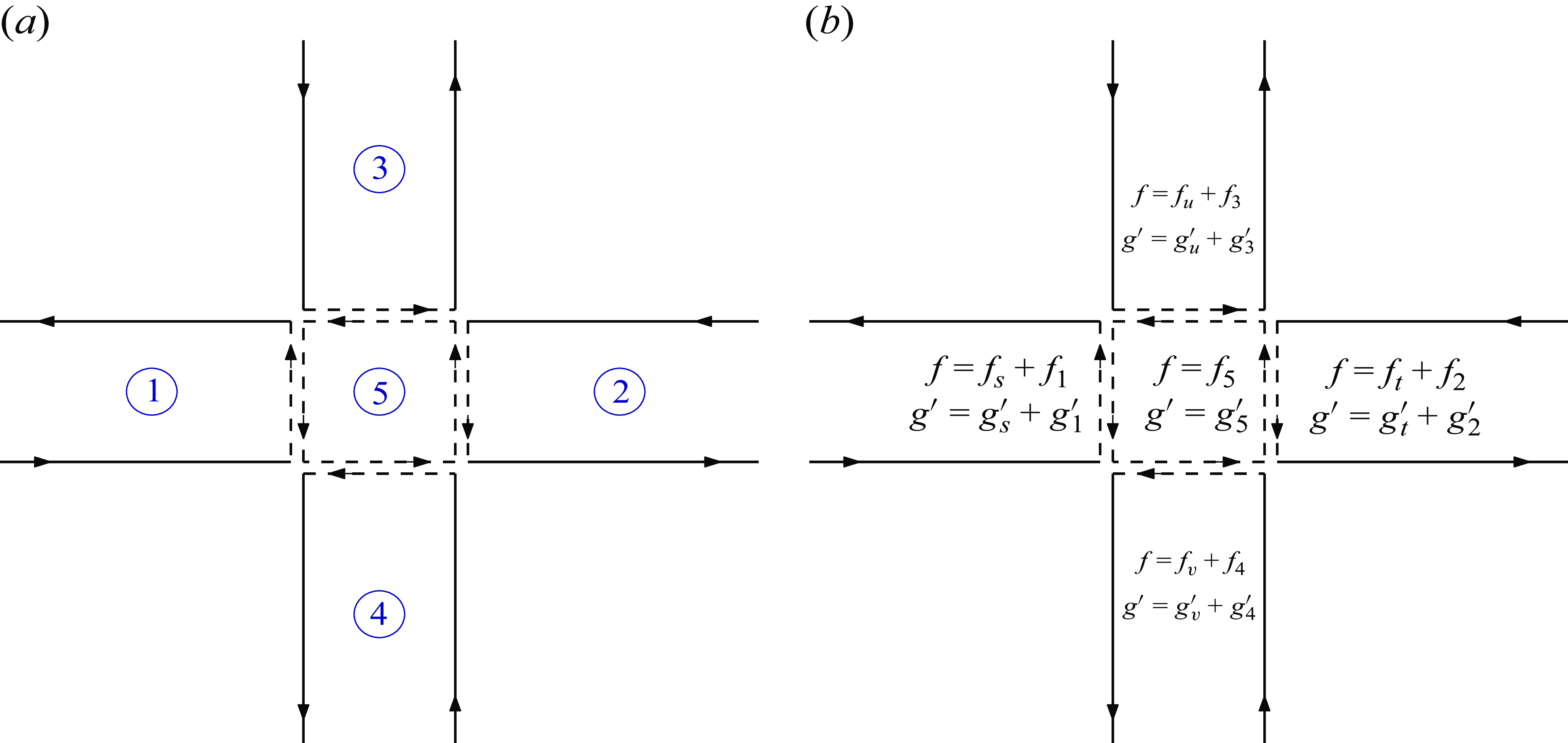


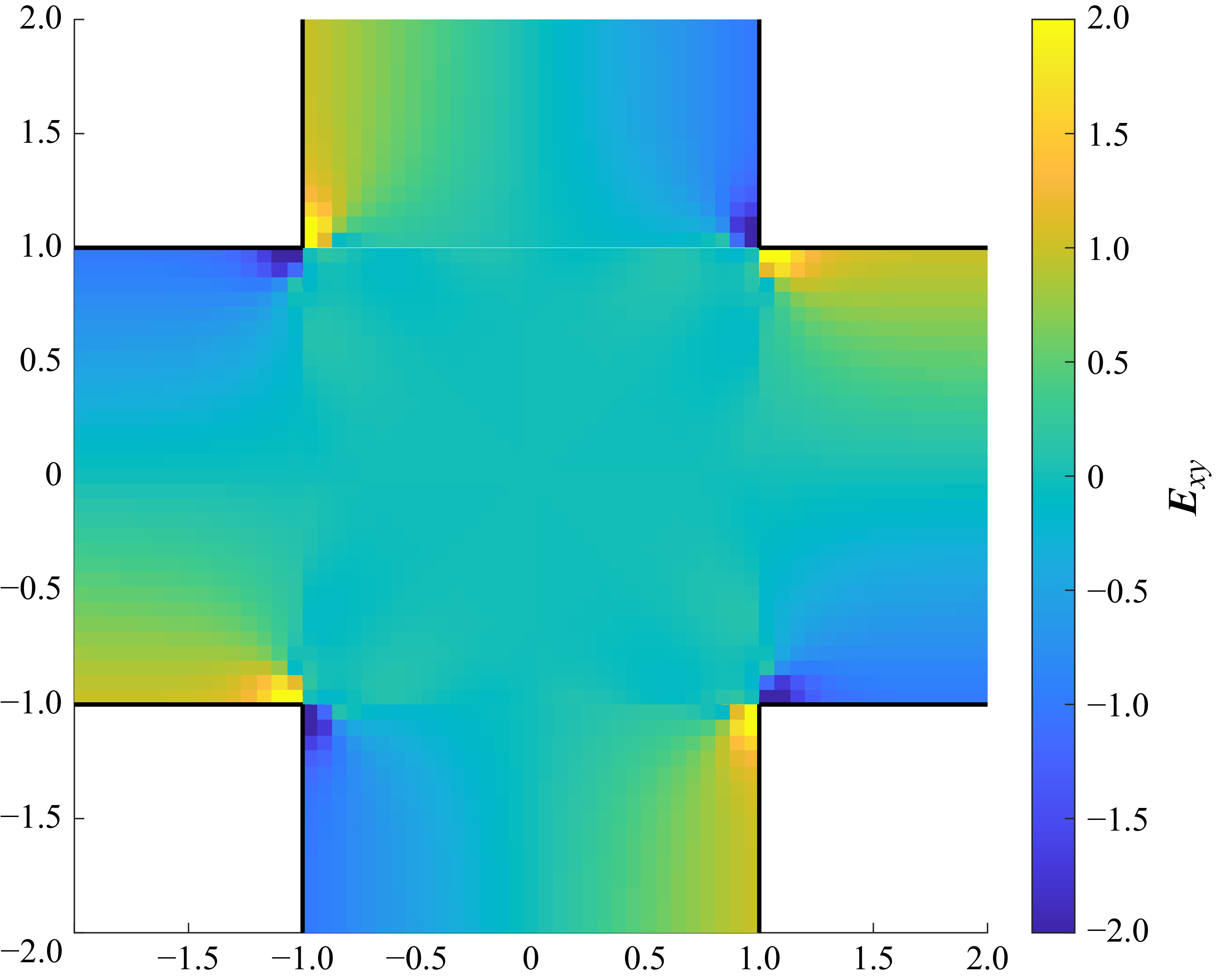

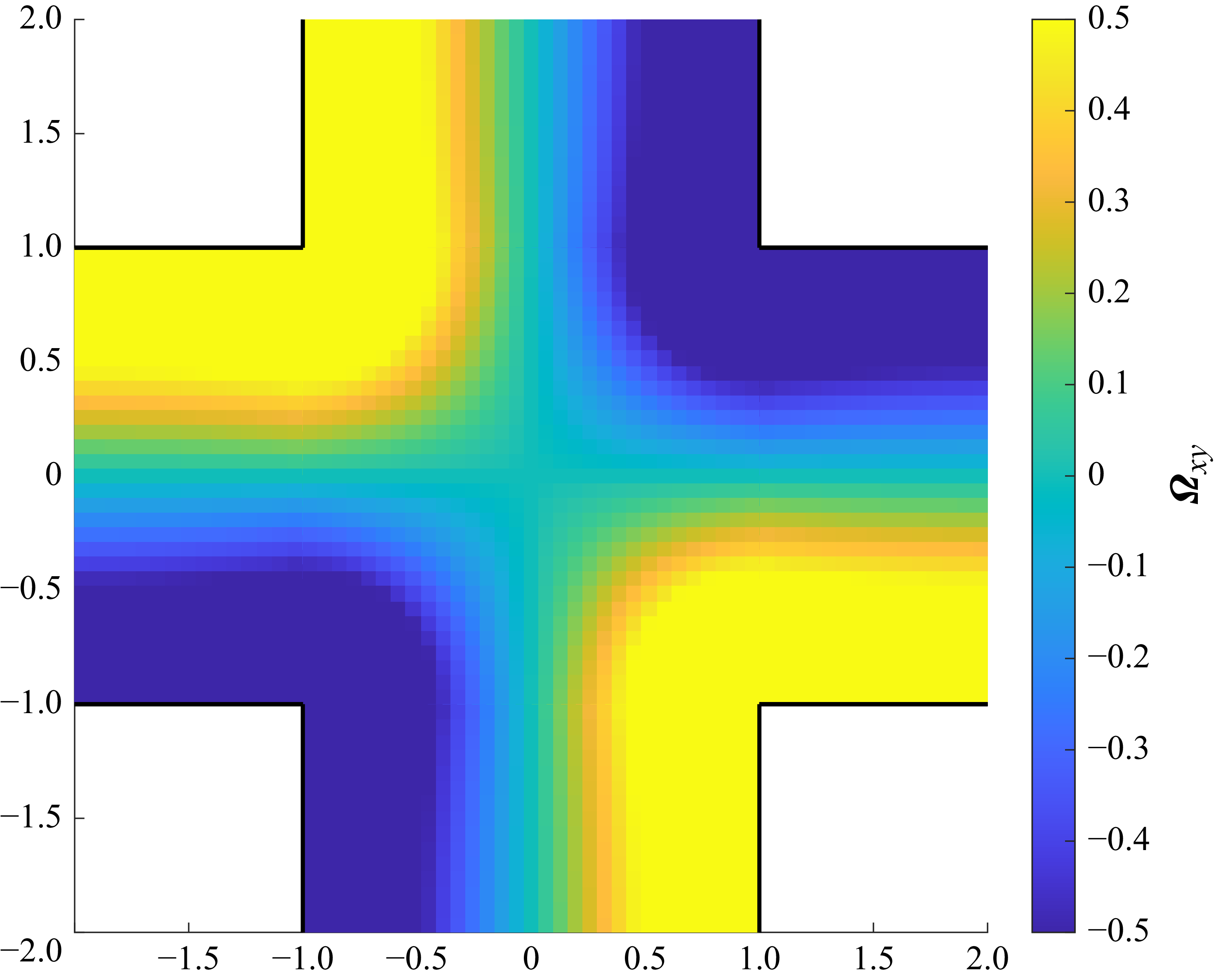

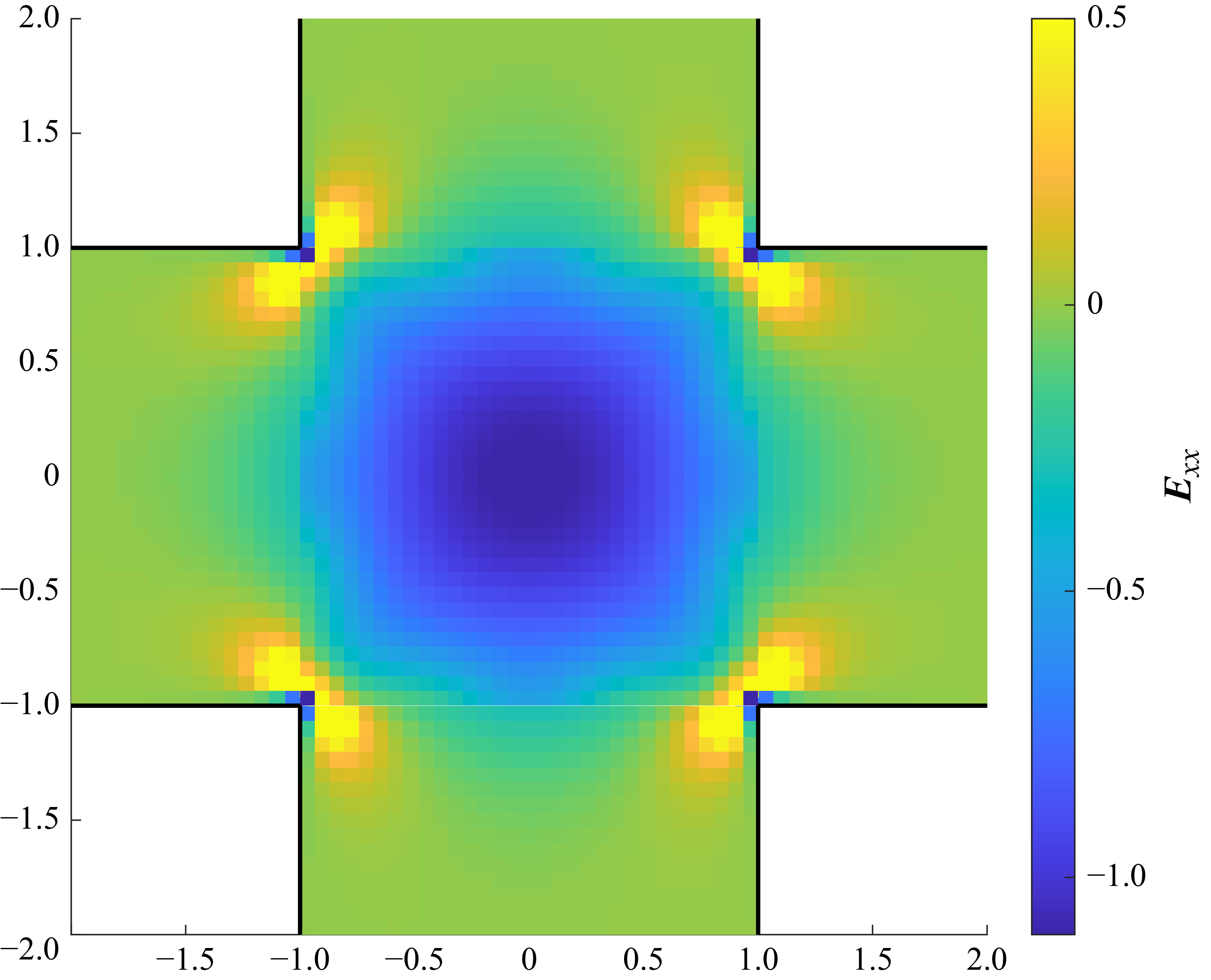

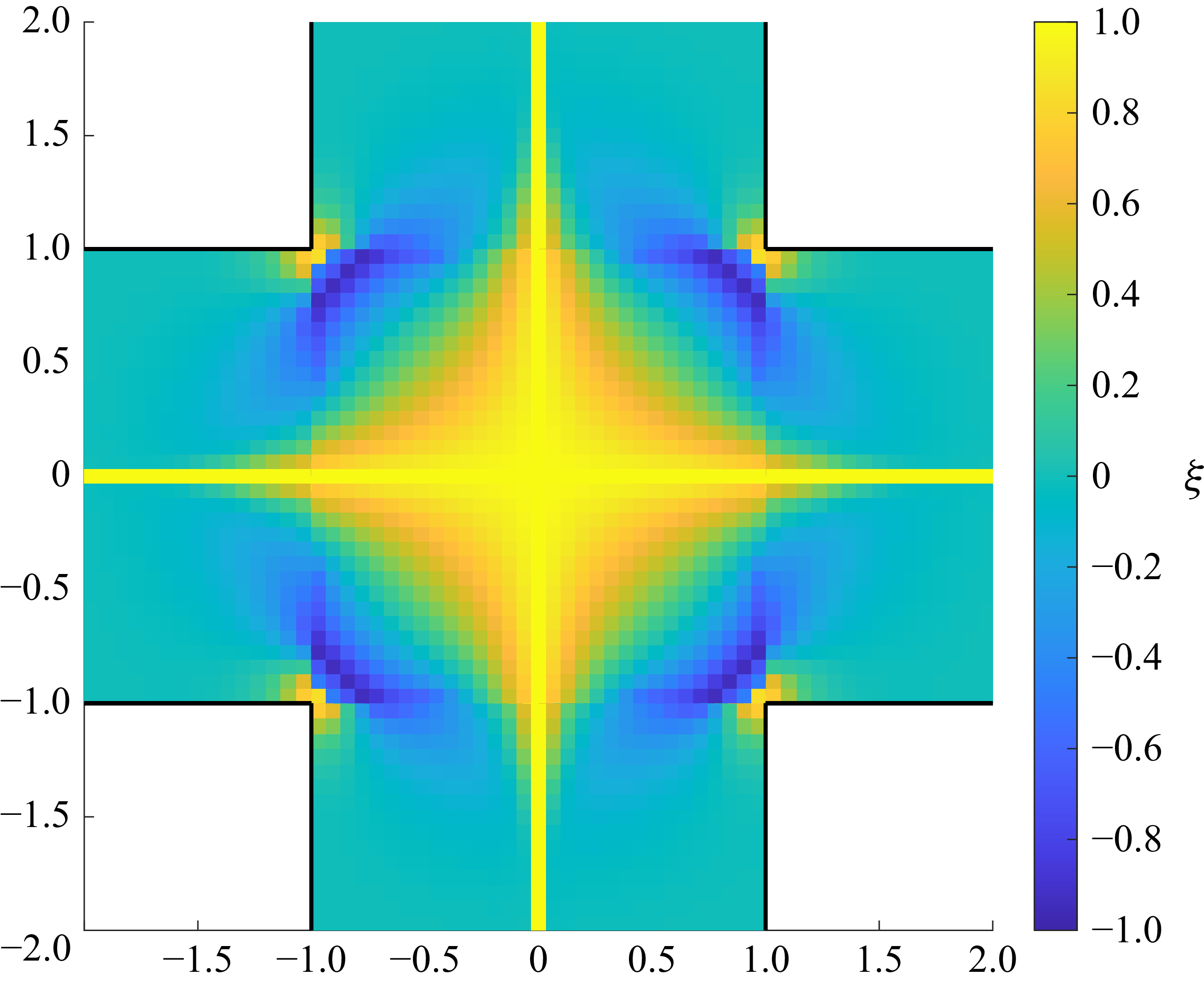


 Open access