


1. Introduction
The transition to a carbon-free energy system will heavily rely on chemical energy carriers like green hydrogen ( $\textrm {H}_{2}$
) to meet the requirements for energy transport and long-term storage (Dreizler et al. Reference Dreizler, Pitsch, Scherer, Schulz and Janicka2021). From an engineering perspective, fuel-lean premixed hydrogen combustion is especially relevant, primarily as it limits thermal
$\textrm {H}_{2}$
) to meet the requirements for energy transport and long-term storage (Dreizler et al. Reference Dreizler, Pitsch, Scherer, Schulz and Janicka2021). From an engineering perspective, fuel-lean premixed hydrogen combustion is especially relevant, primarily as it limits thermal $\textrm {NO}_{x}$
formation (Verhelst & Wallner Reference Verhelst and Wallner2009; Pitsch Reference Pitsch2024). However, lean hydrogen flames are known to be susceptible to intrinsic flame instabilities under operating conditions typical of practical combustion systems, including gas turbines at elevated pressures and temperatures, and domestic heaters at low temperatures and ambient pressure (Berger et al. Reference Berger, Attili and Pitsch2022a
,
Reference Berger, Attili and Pitschb
; Schneider et al. Reference Schneider, Nicolai, Schuh, Steinhausen and Hasse2025a
,
Reference Schneider, Nicolai, Schuh, Steinhausen and Hasseb
).
$\textrm {NO}_{x}$
formation (Verhelst & Wallner Reference Verhelst and Wallner2009; Pitsch Reference Pitsch2024). However, lean hydrogen flames are known to be susceptible to intrinsic flame instabilities under operating conditions typical of practical combustion systems, including gas turbines at elevated pressures and temperatures, and domestic heaters at low temperatures and ambient pressure (Berger et al. Reference Berger, Attili and Pitsch2022a
,
Reference Berger, Attili and Pitschb
; Schneider et al. Reference Schneider, Nicolai, Schuh, Steinhausen and Hasse2025a
,
Reference Schneider, Nicolai, Schuh, Steinhausen and Hasseb
).
Intrinsic flame instabilities comprise hydrodynamic (Darrieus–Landau, DL) instabilities, caused by the density jump across the flame front, and thermodiffusive (TD) instabilities, stemming from the disparity between heat and mass diffusivity, amplified by hydrogen’s high molecular diffusivity (Matalon Reference Matalon2007; Creta et al. Reference Creta, Lapenna, Lamioni, Fogla and Matalon2020). TD instabilities promote local mixture enrichment and burning-rate fluctuations. Furthermore, although TD instabilities are localised effects, they lead to significant acceleration of the global flame speed (Altantzis et al. Reference Altantzis, Frouzakis, Tomboulides, Matalon and Boulouchos2012; Berger et al. Reference Berger, Kleinheinz, Attili and Pitsch2019; Howarth, Hunt & Aspden Reference Howarth, Hunt and Aspden2023), thereby posing challenges to maintain stable flame operation.
Additionally, technical combustion systems are typically confined by walls, leading to flame–wall interactions (FWIs). These interactions potentially increase pollutant formation due to flame quenching and incomplete combustion, while also inducing wall heat fluxes that may lead to material degradation (Dreizler & Böhm Reference Dreizler and Böhm2015). FWIs have been studied mostly in hydrocarbon flames (e.g. Bioche, Vervisch & Ribert Reference Bioche, Vervisch and Ribert2018; Steinhausen et al. Reference Steinhausen2020, Reference Steinhausen, Zirwes, Ferraro, Scholtissek, Bockhorn and Hasse2023) and partially also in hydrogen flames under fuel-rich operating conditions (e.g. Gruber et al. Reference Gruber, Sankaran, Hawkes and Chen2010, Reference Gruber, Chen, Valiev and Law2012; see Dreizler & Böhm (Reference Dreizler and Böhm2015) for a detailed overview). Furthermore, other studies have examined the influence of non-unity Lewis numbers on the quenching process in turbulent HOQ flames (e.g. Lai & Chakraborty Reference Lai and Chakraborty2015; Lai et al. Reference Lai, Ahmed, Klein and Chakraborty2022). Addressing an aspect not covered in previous studies, Schneider et al. (Reference Schneider, Nicolai, Schuh, Steinhausen and Hasse2025a , Reference Schneider, Nicolai, Schuh, Steinhausen and Hasseb ) have demonstrated for the first time that TD instabilities fundamentally alter the quenching behaviour of multidimensional lean premixed (laminar) hydrogen flames, leading to significantly higher wall heat fluxes and markedly shorter quenching distances than a one-dimensional (1D) reference flame under identical conditions.
Toward more application-relevant configurations, simulations that resolve detailed chemical kinetics and transport become increasingly complex and may become prohibitively expensive or even practically infeasible (Fiorina, Veynante & Candel Reference Fiorina, Veynante and Candel2014). This motivates the use of reduced-order models, among which tabulated chemistry (TC) methods offer particularly high computational efficiency (Fiorina et al. Reference Fiorina, Veynante and Candel2014; van Oijen et al. Reference van Oijen, Donini, Bastiaans, ten Thije Boonkkamp and de Goey2016). These methods rely on the assumption that the thermochemical state of the flame resides on a lower-dimensional manifold, typically derived from 1D laminar flame simulations and parametrised by a set of reduced control variables $\mathcal{Y}_i$
. This allows for only solving the transport equations for
$\mathcal{Y}_i$
. This allows for only solving the transport equations for $\mathcal{Y}_i$
at runtime and retrieving the corresponding thermochemical state directly from the manifold. Various tabulation strategies, such as flame prolongation of intrinsic low-dimensional manifold method (Gicquel, Darabiha & Thévenin Reference Gicquel, Darabiha and Thévenin2000), the flamelet–progress variable (FPV) method (Pierce & Moin Reference Pierce and Moin2004) and flamelet-generated manifolds (FGM) (Oijen & Goey Reference Oijen van and Goey de2000; van Oijen et al. Reference van Oijen, Donini, Bastiaans, ten Thije Boonkkamp and de Goey2016), have been successfully developed for hydrocarbon fuels and shown to yield accurate results even in complex configurations.
$\mathcal{Y}_i$
at runtime and retrieving the corresponding thermochemical state directly from the manifold. Various tabulation strategies, such as flame prolongation of intrinsic low-dimensional manifold method (Gicquel, Darabiha & Thévenin Reference Gicquel, Darabiha and Thévenin2000), the flamelet–progress variable (FPV) method (Pierce & Moin Reference Pierce and Moin2004) and flamelet-generated manifolds (FGM) (Oijen & Goey Reference Oijen van and Goey de2000; van Oijen et al. Reference van Oijen, Donini, Bastiaans, ten Thije Boonkkamp and de Goey2016), have been successfully developed for hydrocarbon fuels and shown to yield accurate results even in complex configurations.
In recent years, extensions of TC approaches to FWIs have been intensively investigated in laminar and turbulent side-wall quenching (SWQ) configurations to improve pollutant predictions in hydrocarbon flames (Ganter et al. Reference Ganter, Heinrich, Meier, Kuenne, Jainski, Rißmann, Dreizler and Janicka2017, Reference Ganter, Straßacker, Kuenne, Meier, Heinrich, Maas and Janicka2018; Efimov, de Goey & van Oijen Reference Efimov, de Goey and van Oijen2019; Steinhausen et al. Reference Steinhausen2020, Reference Steinhausen, Zirwes, Ferraro, Scholtissek, Bockhorn and Hasse2023). These studies demonstrated that manifolds based on head-on quenching (HOQ) flamelets offer superior accuracy, particularly regarding CO formation, compared with those based on freely propagating (FP) flames with varying levels of enthalpy, as usually employed to capture heat losses in lifted flames (Ketelheun, Kuenne & Janicka Reference Ketelheun, Kuenne and Janicka2013). However, these studies focus exclusively on hydrocarbon fuels, where differential and preferential diffusion effects are typically assumed to be negligible. As a result, the unity Lewis number assumption is commonly applied in both manifold generation and the transport equations with minimal impact on the model accuracy (Ganter et al. Reference Ganter, Heinrich, Meier, Kuenne, Jainski, Rißmann, Dreizler and Janicka2017). Note that in the following, the term differential diffusion comprises both differential diffusion through the disparity of heat and species diffusion (i.e. non-unity Lewis numbers) and preferential diffusion between individual species (i.e. non-equal Lewis numbers).
In contrast, assuming a unity Lewis number in hydrogen combustion artificially suppresses differential diffusion effects and thereby predicts incorrect flame properties, such as flame speeds and flame thicknesses, and, most critically, fails to capture TD instabilities. To overcome this limitation, in recent years, a number of studies (de Swart et al. Reference de Swart, Bastiaans, van Oijen, de Goey and Cant2010; Regele et al. Reference Regele, Knudsen, Pitsch and Blanquart2013; Abtahizadeh, de Goey & van Oijen Reference Abtahizadeh, de Goey and van Oijen2015; Donini et al. Reference Donini, Bastiaans, van Oijen and de Goey2015; Schlup & Blanquart Reference Schlup and Blanquart2019; Mukundakumar et al. Reference Mukundakumar, Efimov, Beishuizen and van Oijen2021; Böttler et al. Reference Böttler, Chen, Xie, Scholtissek, Chen and Hasse2022; Nicolai et al. Reference Nicolai, Dressler, Janicka and Hasse2022; Böttler et al. Reference Böttler, Lulic, Steinhausen, Wen, Hasse and Scholtissek2023, Reference Böttler, Kaddar, Karpowski, Federica, Scholtissek, Nicolai and Hasse2024; Fortes et al. Reference Fortes, Pérez-Sánchez, Both, Grenga and Mira2025; Pérez-Sánchez et al. Reference Pérez-Sánchez, Fortes and Mira2025; Schepers & van Oijen Reference Schepers and van Oijen2025) have extended TC approaches to capture differential diffusion effects in premixed hydrogen flames. While some studies focus on TD instabilities and others on heat losses, none simultaneously address both effects with explicit consideration of FWIs, a critical gap given their coupled impact in practical combustion systems.
Accordingly, to provide reliable reduced-order simulations of near-wall TD instabilities, the objectives of this work are as follows:
-
(i) To develop an accurate TC model for the FWI of TD unstable $\textrm {H}_{2}$
/air flames, advancing a recently proposed flamelet tabulation framework by Abtahizadeh et al. (Reference Abtahizadeh, de Goey and van Oijen2015), Nicolai et al. (Reference Nicolai, Dressler, Janicka and Hasse2022); Pérez-Sánchez et al. (Reference Pérez-Sánchez, Fortes and Mira2025).
$\textrm {H}_{2}$
/air flames, advancing a recently proposed flamelet tabulation framework by Abtahizadeh et al. (Reference Abtahizadeh, de Goey and van Oijen2015), Nicolai et al. (Reference Nicolai, Dressler, Janicka and Hasse2022); Pérez-Sánchez et al. (Reference Pérez-Sánchez, Fortes and Mira2025). -
(ii) To derive a universal approach for accurately and efficiently determining the additional terms in the transport equations resulting from differential diffusion.
-
(iii) To incorporate thermal (Soret) diffusion into the flamelet tabulation framework, acknowledging its significant role in lean hydrogen combustion, including the near-wall regions (Schlup & Blanquart Reference Schlup and Blanquart2017, Reference Schlup and Blanquart2018; Zirwes et al. Reference Zirwes, Zhang, Kaiser, Oberleithner, Stein, Bockhorn and Kronenburg2024).
-
(iv) To examine two different flamelet databases: one derived from 1D FP flames with enthalpy variation, and another based on 1D HOQ flamelets, which have demonstrated superior accuracy for hydrocarbon flames.
-
(v) To validate the framework and the manifolds in both an a-priori and a-posteriori manner against reference detailed chemistry (DC) simulations.

The remainder of this work is structured as follows: § 2 presents the flamelet tabulation approach, highlighting the novel extensions introduced in this work beyond the base model, with a particular focus on the formulation and computation of additional terms capturing differential diffusion effects. Section 3 outlines the numerical methods used, while § 4 introduces the different manifolds employed in this study, targeting either TD instabilities or heat losses. Furthermore, a combination of these manifolds into joint manifolds is developed to simultaneously capture both effects. Subsequently, § 5 evaluates the manifolds across a sequence of increasingly complex configurations: 1D FP flames for model verification; 1D HOQ flames to assess the model’s capabilities to capture heat losses; two-dimensional (2D) TD unstable flames to assess the model’s capabilities to capture TD instabilities and, finally, 2D HOQ of a thermodiffusively unstable flame, which demands that the manifolds simultaneously capture both instabilities and heat losses. In this context, both a-priori analyses and a-posteriori evaluations based on fully coupled TC simulations are conducted and compared against DC reference simulations. The paper concludes with a summary and outlook in § 6.
2. Differential diffusion in TC models: background and model extensions
Various TC modelling approaches from the literature are first briefly summarised to demonstrate the foundation of the proposed model and to contextualise its differences from other model formulations. Subsequently, the TC model employed in this study is derived in detail and the manifold construction is outlined.
2.1. Model background and classification
To incorporate differential diffusion, various approaches have been proposed in the literature (Oijen & Goey Reference Oijen van and Goey de2000; Vreman et al. Reference Vreman, van Oijen, de Goey and Bastiaans2009; de Swart et al. Reference de Swart, Bastiaans, van Oijen, de Goey and Cant2010; Regele et al. Reference Regele, Knudsen, Pitsch and Blanquart2013; Abtahizadeh et al. Reference Abtahizadeh, de Goey and van Oijen2015; Böttler et al. Reference Böttler, Scholtissek, Chen, Chen and Hasse2021; Nicolai et al. Reference Nicolai, Dressler, Janicka and Hasse2022; Pérez-Sánchez et al. Reference Pérez-Sánchez, Fortes and Mira2025). All these models within the TC framework have in common that they are constructed from precomputed flamelets (see van Oijen et al. Reference van Oijen, Donini, Bastiaans, ten Thije Boonkkamp and de Goey2016 for details) and employ a reaction progress variable $Y_{{c}}$
as one of the controlling variables of the manifolds, typically defined as a linear combination of species mass fractions:
$Y_{{c}}$
as one of the controlling variables of the manifolds, typically defined as a linear combination of species mass fractions:
 \begin{equation} Y_{{c}} = \sum _{k=1}^{N_{{s}}} a_k Y_k . \end{equation}
Here $a_k$
is the weighting factor associated with the mass fraction
$a_k$
is the weighting factor associated with the mass fraction $Y_k$
of species
$Y_k$
of species $k$
. The transport equation for the progress variable can be derived from the species transport equation. The general form of the transport equation for a species mass fraction
$k$
. The transport equation for the progress variable can be derived from the species transport equation. The general form of the transport equation for a species mass fraction $Y_k$
is given by
$Y_k$
is given by
 \begin{equation} \frac {\partial \rho Y_k}{\partial t} + \frac {\partial \rho u_i Y_k}{\partial x_i} = - \frac {\partial \rho Y_k V_{k,i}}{\partial x_i} + \dot {\omega }_k, \quad k=1,\ldots ,N_{{s}} , \end{equation}
where $u_i$
is the velocity in direction
$u_i$
is the velocity in direction $i$
,
$i$
, $V_{k,i}$
is the diffusion velocity of species
$V_{k,i}$
is the diffusion velocity of species $k$
in direction
$k$
in direction $i$
,
$i$
, $\rho$
is the density and
$\rho$
is the density and $\dot {\omega }_k$
is the reaction source term of species
$\dot {\omega }_k$
is the reaction source term of species $k$
. An equation for the progress variable
$k$
. An equation for the progress variable $Y_{{c}}$
follows by summing the species transport equations, weighted by
$Y_{{c}}$
follows by summing the species transport equations, weighted by $a_k$
:
$a_k$
:
 \begin{equation} \frac {\partial \rho Y_{{c}}}{\partial t} + \frac {\partial \rho u_i Y_{{c}}}{\partial x_i} = -\frac {\partial }{\partial x_i}\! \left ( \rho \sum _{k=1}^{N_{{s}}} a_k Y_k V_{k,i} \right ) + \sum _{k=1}^{N_{{s}}} a_k \dot {\omega }_k. \end{equation}
Notably, the diffusion term involves a summation over the diffusion fluxes of all species contributing to the progress variable, which necessitates an appropriate closure. In contrast, assuming a unity Lewis number implies identical diffusion coefficients for all species, which can be factored out of the summation, thereby enabling an analytical closure of the term.
When differential diffusion becomes important, the multidimensional flame structure can deviate from a 1D profile due to flame front curvature, and might therefore vary locally. Thus, even in a purely premixed flame, multidimensional diffusion effects emerge, with transport occurring not only normal to the flame front but also tangential to it. As a result, the thermochemical state cannot be represented by a single controlling variable (de Swart et al. Reference de Swart, Bastiaans, van Oijen, de Goey and Cant2010; Regele et al. Reference Regele, Knudsen, Pitsch and Blanquart2013). Thus, theoretically, to take differential diffusion into account in a three-element system (H, O, N), in addition to the reaction progress variable $Y_{{c}}$
, two elemental mass fractions, e.g.
$Y_{{c}}$
, two elemental mass fractions, e.g. $Z_{\textrm {H}}$
and
$Z_{\textrm {H}}$
and $Z_{\textrm {O}}$
(since the missing elemental mass fraction is determined from the element mass fraction unity constraint), are required to capture the local elemental composition and chemical equilibrium (de Swart et al. Reference de Swart, Bastiaans, van Oijen, de Goey and Cant2010; Nicolai et al. Reference Nicolai, Dressler, Janicka and Hasse2022). In this context, elemental mass fractions (and mixture fractions in general) offer the key advantage for TC approaches that they are conserved during chemical reactions and, consequently, their transport equations contain no chemical source terms.
$Z_{\textrm {O}}$
(since the missing elemental mass fraction is determined from the element mass fraction unity constraint), are required to capture the local elemental composition and chemical equilibrium (de Swart et al. Reference de Swart, Bastiaans, van Oijen, de Goey and Cant2010; Nicolai et al. Reference Nicolai, Dressler, Janicka and Hasse2022). In this context, elemental mass fractions (and mixture fractions in general) offer the key advantage for TC approaches that they are conserved during chemical reactions and, consequently, their transport equations contain no chemical source terms.
The elemental mass fraction of an element $e$
is defined as
$e$
is defined as
 \begin{equation} Z_{e} = \sum _{k=1}^{N_{{s}}} \gamma _{e,k} \frac {W_e}{W_k} Y_k, \end{equation}
where $\gamma _{e,k}$
is the number of atoms of element
$\gamma _{e,k}$
is the number of atoms of element $e$
in species
$e$
in species $k$
, and
$k$
, and $W_e$
and
$W_e$
and $W_k$
are the molar masses of element
$W_k$
are the molar masses of element $e$
and species
$e$
and species $k$
, respectively. Summing the species transport equations according to (2.4), the elemental mass fraction transport equation is obtained:
$k$
, respectively. Summing the species transport equations according to (2.4), the elemental mass fraction transport equation is obtained:
 \begin{equation} \frac {\partial \rho Z_e}{\partial t} + \frac {\partial \rho u_i Z_e}{\partial x_i} = -\frac {\partial }{\partial x_i}\! \left ( \rho \sum _{k=1}^{N_{{s}}} \gamma _{e,k} \frac {W_e}{W_k} Y_k V_{k,i} \right )\!. \end{equation}
Note that the same considerations also apply to other definitions of mixture fractions, for example, $Z_{\textit{Bilger}}$
, which is defined as a normalised linear combination of elemental mass fractions, allowing a corresponding transport equation to be derived, as detailed by Pérez-Sánchez et al. (Reference Pérez-Sánchez, Fortes and Mira2025). The diffusion term in the transport equation(s) of the elemental mass fractions(s) (or mixture fraction(s)) also requires closure, as it involves the summation of the diffusive fluxes of multiple species. To simplify this, many studies adopt a reduced mixture fraction, though its definition often varies. Furthermore, to limit the number of controlling variables, which is computationally unfavourable, the dimensionality is often reduced by assuming a relation between the elemental mass fractions (and enthalpy) (de Swart et al. Reference de Swart, Bastiaans, van Oijen, de Goey and Cant2010; Nicolai et al. Reference Nicolai, Kuenne, Knappstein, Schneider, Becker, Hasse, Mare, di Dreizler and Janicka2020).
$Z_{\textit{Bilger}}$
, which is defined as a normalised linear combination of elemental mass fractions, allowing a corresponding transport equation to be derived, as detailed by Pérez-Sánchez et al. (Reference Pérez-Sánchez, Fortes and Mira2025). The diffusion term in the transport equation(s) of the elemental mass fractions(s) (or mixture fraction(s)) also requires closure, as it involves the summation of the diffusive fluxes of multiple species. To simplify this, many studies adopt a reduced mixture fraction, though its definition often varies. Furthermore, to limit the number of controlling variables, which is computationally unfavourable, the dimensionality is often reduced by assuming a relation between the elemental mass fractions (and enthalpy) (de Swart et al. Reference de Swart, Bastiaans, van Oijen, de Goey and Cant2010; Nicolai et al. Reference Nicolai, Kuenne, Knappstein, Schneider, Becker, Hasse, Mare, di Dreizler and Janicka2020).
In summary, existing models differ notably in how they treat diffusion, leading to variations not only in the definition of the mixture fraction but, in some cases, also in the flamelet database. These distinctions are examined in more detail through a review of the respective modelling strategies found in the literature.
2.1.1. Simplified mixture fraction models
Initial efforts to capture differential diffusion effects were conducted by Vreman et al. (Reference Vreman, van Oijen, de Goey and Bastiaans2009), who computed an effective Lewis number for each controlling variable. Their approach accounted for differential diffusion between heat and fuel but did not capture preferential diffusion between individual species. Moreover, the results were found to be sensitive to the choice of controlling variables.
Another approach to capture differential and preferential diffusion was proposed by Regele et al. (Reference Regele, Knudsen, Pitsch and Blanquart2013), who extended the FPV model to incorporate constant, non-unity Lewis numbers. They employed a reduced mixture fraction that considers only fuel and oxidiser, and assumed one-step chemistry for the derivation of its transport equation. This offers the advantage of a simplified closure of the diffusion terms, however, only the diffusion effects of the major species are taken into account. Note that the mixture fraction transport equation includes a cross-diffusion term that accounts for diffusion induced by the gradient of the progress variable. However, no corresponding cross-diffusion term is included in the progress variable transport equation. The authors employed a flamelet database consisting of 1D FP flames with varying equivalence ratios. Schlup & Blanquart (Reference Schlup and Blanquart2019) extended the work by Regele et al. (Reference Regele, Knudsen, Pitsch and Blanquart2013) and relaxed the constant Lewis number assumption to include mixture-averaged transport and thermal (Soret) diffusion. The model was tested on a spherically expanding flame and a TD unstable FP flame, both showing good results. A three-dimensional (3D) simulation of a turbulent premixed lean hydrogen/air flame showed good agreement in regions without superadiabatic temperatures, but deviations were observed in superadiabatic regions. Yao & Blanquart (Reference Yao and Blanquart2024) applied this model in the framework of the large eddy simulations (LES) of a low-swirl burner with a lean premixed hydrogen/air mixture using a presumed probability density function (PDF) approach for turbulence-chemistry interaction (TCI), while Berger et al. (Reference Berger, Attili, Gauding and Pitsch2025) also applied the model in the LES of a lean hydrogen/air slot flame also using a presumed PDF approach for TCI.
Böttler et al. (Reference Böttler, Chen, Xie, Scholtissek, Chen and Hasse2022, Reference Böttler, Lulic, Steinhausen, Wen, Hasse and Scholtissek2023) adopted an approach conceptually similar to that of Regele et al. (Reference Regele, Knudsen, Pitsch and Blanquart2013) and Schlup & Blanquart (Reference Schlup and Blanquart2019), employing a reduced mixture fraction based on the major species ( $\textrm {H}_{2}$
,
$\textrm {H}_{2}$
, $\textrm {O}_{2}$
and
$\textrm {O}_{2}$
and ${\textrm {H}_{2}}\textrm {O}$
). However, instead of directly transporting this reduced mixture fraction, they solved transport equations for the major species and reconstructed both the reduced mixture fraction and the progress variable from those species prior to the table lookup. In the transport equations of the major species, the diffusion coefficients of the transported species are well defined and can be tabulated directly. The correction velocity and thermal diffusion are neglected in the transport equations, as their closure is not straightforward within this framework. As the model was originally developed for forced ignition in hydrogen/air mixtures (Böttler et al. Reference Böttler, Chen, Xie, Scholtissek, Chen and Hasse2022), a transport equation for the enthalpy
${\textrm {H}_{2}}\textrm {O}$
). However, instead of directly transporting this reduced mixture fraction, they solved transport equations for the major species and reconstructed both the reduced mixture fraction and the progress variable from those species prior to the table lookup. In the transport equations of the major species, the diffusion coefficients of the transported species are well defined and can be tabulated directly. The correction velocity and thermal diffusion are neglected in the transport equations, as their closure is not straightforward within this framework. As the model was originally developed for forced ignition in hydrogen/air mixtures (Böttler et al. Reference Böttler, Chen, Xie, Scholtissek, Chen and Hasse2022), a transport equation for the enthalpy $h$
was included, resulting in a 3D manifold with
$h$
was included, resulting in a 3D manifold with $Y_{{c}}$
,
$Y_{{c}}$
, $Z$
and
$Z$
and $h$
as controlling variables. For the differential diffusion term in the enthalpy equation, the gradients of the non-transported species were approximated using the corresponding gradients in the 1D flamelets. Instead of 1D FP unstretched flamelets, the composition space model (CSM) (Scholtissek et al. Reference Scholtissek, Domingo, Vervisch and Hasse2019a
,
Reference Scholtissek, Domingo, Vervisch and Hasseb
) was used for generating the flamelet database, enabling the representation of flame structures from various canonical premixed flame configurations, including arbitrary combinations of strain and curvature (Böttler et al. Reference Böttler, Scholtissek, Chen, Chen and Hasse2021). The model was applied to a spherically expanding TD unstable lean hydrogen/air flame and compared with a second model, also based on the CSM, in which the mixture fraction and the curvature of the flamelets have been varied (Böttler et al. Reference Böttler, Lulic, Steinhausen, Wen, Hasse and Scholtissek2023). Instead of using curvature directly as a controlling variable, the H radical was employed as a second progress variable, resulting in a 3D manifold with a reduced mixture fraction and two progress variables. The newly proposed model showed improved accuracy for TD unstable flames, although discrepancies with DC simulations remain. Schepers & van Oijen (Reference Schepers and van Oijen2025) effectively combined the two aforementioned models and replaced the major species
$h$
as controlling variables. For the differential diffusion term in the enthalpy equation, the gradients of the non-transported species were approximated using the corresponding gradients in the 1D flamelets. Instead of 1D FP unstretched flamelets, the composition space model (CSM) (Scholtissek et al. Reference Scholtissek, Domingo, Vervisch and Hasse2019a
,
Reference Scholtissek, Domingo, Vervisch and Hasseb
) was used for generating the flamelet database, enabling the representation of flame structures from various canonical premixed flame configurations, including arbitrary combinations of strain and curvature (Böttler et al. Reference Böttler, Scholtissek, Chen, Chen and Hasse2021). The model was applied to a spherically expanding TD unstable lean hydrogen/air flame and compared with a second model, also based on the CSM, in which the mixture fraction and the curvature of the flamelets have been varied (Böttler et al. Reference Böttler, Lulic, Steinhausen, Wen, Hasse and Scholtissek2023). Instead of using curvature directly as a controlling variable, the H radical was employed as a second progress variable, resulting in a 3D manifold with a reduced mixture fraction and two progress variables. The newly proposed model showed improved accuracy for TD unstable flames, although discrepancies with DC simulations remain. Schepers & van Oijen (Reference Schepers and van Oijen2025) effectively combined the two aforementioned models and replaced the major species $\textrm {O}_{2}$
with the
$\textrm {O}_{2}$
with the $\textrm {H}$
radical. This substitution is motivated by the significant contribution of the
$\textrm {H}$
radical. This substitution is motivated by the significant contribution of the $\textrm {H}$
radical to the differential diffusion of enthalpy. To construct their model, they employed a flamelet database generated from 1D FP flames with varying enthalpy and mixture fraction levels. Their approach demonstrated improved accuracy when applied to a 2D TD unstable FP flame, while discrepancies remain, for example, in the linear regime of TD instabilities.
$\textrm {H}$
radical to the differential diffusion of enthalpy. To construct their model, they employed a flamelet database generated from 1D FP flames with varying enthalpy and mixture fraction levels. Their approach demonstrated improved accuracy when applied to a 2D TD unstable FP flame, while discrepancies remain, for example, in the linear regime of TD instabilities.
2.1.2. Full mixture fraction models
In contrast, the foundation for the framework presented in this study, originally proposed by Oijen & Goey (Reference Oijen van and Goey de2000) and de Swart et al. (Reference de Swart, Bastiaans, van Oijen, de Goey and Cant2010) within the FGM framework (van Oijen et al. Reference van Oijen, Donini, Bastiaans, ten Thije Boonkkamp and de Goey2016), is not based on a reduced mixture fraction definition. In their formulation, constant Lewis numbers were assumed (i.e. $\textit{Le}_i$
does not vary across the flame front). They demonstrated that, under the manifold assumption, i.e. that any quantity
$\textit{Le}_i$
does not vary across the flame front). They demonstrated that, under the manifold assumption, i.e. that any quantity $\xi$
depends solely on the controlling variables, the diffusion terms in the transport equations of the controlling variable can be closed, as illustrated through the following considerations.
$\xi$
depends solely on the controlling variables, the diffusion terms in the transport equations of the controlling variable can be closed, as illustrated through the following considerations.
While diffusion terms could be computed directly during simulation using the manifold, this would require storing all species mass fractions and diffusion coefficients, causing significant memory and computational overhead. Instead, gradients are partially precomputed in the manifold, greatly reducing the number of variables retrieved from the table. For any manifold quantity $\xi (\mathcal{Y}_1, \ldots , \mathcal{Y}_n)$
(e.g. a species mass fraction
$\xi (\mathcal{Y}_1, \ldots , \mathcal{Y}_n)$
(e.g. a species mass fraction $Y_k$
), the total differential is defined as
$Y_k$
), the total differential is defined as
 \begin{equation} \frac {\partial \xi }{\partial x_i} = \sum _{j=1}^{N_{{c}}} \left .\frac {\partial \xi }{\partial \mathcal{Y}_{\!j}}\right |_{\mathcal{Y}_1,\ldots ,\mathcal{Y}_{j-1},\mathcal{Y}_{j+1},\ldots ,\mathcal{Y}_{n}} \frac {\partial \mathcal{Y}_{\!j}}{\partial x_i}, \end{equation}
where gradients with respect to the controlling variables $\mathcal{Y}_{\!j}$
are precomputed within the manifold, while spatial gradients of the controlling variables are obtained during the simulation. (Note that in the following,
$\mathcal{Y}_{\!j}$
are precomputed within the manifold, while spatial gradients of the controlling variables are obtained during the simulation. (Note that in the following, $\left .{\partial \xi }/{\partial \mathcal{Y}_{\!j}}\right |_{\mathcal{Y}_1,\ldots ,\mathcal{Y}_{j-1},\mathcal{Y}_{j+1},\ldots ,\mathcal{Y}_{n}}$
is abbreviated as
$\left .{\partial \xi }/{\partial \mathcal{Y}_{\!j}}\right |_{\mathcal{Y}_1,\ldots ,\mathcal{Y}_{j-1},\mathcal{Y}_{j+1},\ldots ,\mathcal{Y}_{n}}$
is abbreviated as ${\partial \xi }/{\partial \mathcal{Y}_{\!j}}$
.) Various approaches exist for this purpose, and the method employed in this work for calculating the gradients with respect to the controlling variables is discussed in detail in the following section. Assuming constant Lewis numbers, the diffusion flux is defined as
${\partial \xi }/{\partial \mathcal{Y}_{\!j}}$
.) Various approaches exist for this purpose, and the method employed in this work for calculating the gradients with respect to the controlling variables is discussed in detail in the following section. Assuming constant Lewis numbers, the diffusion flux is defined as $Y_{k} V_{k,i} = - {\alpha }/{{\textit{Le}_k}}\,{\partial Y_k}/{\partial x_i}$
, which can be reformulated as
$Y_{k} V_{k,i} = - {\alpha }/{{\textit{Le}_k}}\,{\partial Y_k}/{\partial x_i}$
, which can be reformulated as $Y_k V_{k,i} = - \sum _{l=1}^{N_{{c}}} ({\alpha }/{\textit{Le}_k} \, {\partial Y_k}{/\partial \mathcal{Y}_l}) {\partial \mathcal{Y}_l} / \partial x_i = - \sum _{l=1}^{N_{{c}}} \varLambda _{Y_k,\mathcal{Y}_l} \partial \mathcal{Y}_{l} / \partial x_i$
using (2.6).
$Y_k V_{k,i} = - \sum _{l=1}^{N_{{c}}} ({\alpha }/{\textit{Le}_k} \, {\partial Y_k}{/\partial \mathcal{Y}_l}) {\partial \mathcal{Y}_l} / \partial x_i = - \sum _{l=1}^{N_{{c}}} \varLambda _{Y_k,\mathcal{Y}_l} \partial \mathcal{Y}_{l} / \partial x_i$
using (2.6).
For an exemplary controlling variable $\mathcal{Y}_{\!j}$
, the transport equation is given by
$\mathcal{Y}_{\!j}$
, the transport equation is given by
 \begin{equation} \frac {\partial \rho \mathcal{Y}_{\!j}}{\partial t} + \frac {\partial \rho u_i \mathcal{Y}_{\!j}}{\partial x_i} = \frac {\partial }{\partial x_i}\! \left (\rho \sum _{k=1}^{N_{{s}}} \varsigma _{j,k} Y_k V_{k,i} \right ) + S_{\mathcal{Y}_{\!j}}, \end{equation}
with the source term $S_{\mathcal{Y}_{\!j}}$
and the weighting factor
$S_{\mathcal{Y}_{\!j}}$
and the weighting factor $\varsigma _{j,k}$
of species
$\varsigma _{j,k}$
of species $k$
associated with the controlling variable
$k$
associated with the controlling variable $\mathcal{Y}_{\!j}$
, which, for example, corresponds to the weighting factor
$\mathcal{Y}_{\!j}$
, which, for example, corresponds to the weighting factor $a_{k}$
in the case of a reaction progress variable. The diffusion term in the
$a_{k}$
in the case of a reaction progress variable. The diffusion term in the $\mathcal{Y}_{\!j}$
transport equation can be reformulated as
$\mathcal{Y}_{\!j}$
transport equation can be reformulated as
 \begin{align} - \rho \sum _{k=1}^{N_{{s}}} \varsigma _{j,k} Y_k V_{k,i} = \rho \sum _{k=1}^{N_{{s}}} \varsigma _{j,k}\! \left (-Y_k V_{k,i}\right ) - \frac {\kappa }{c_p} \frac {\partial \mathcal{Y}_{\!j}}{\partial x_i} + \frac {\kappa }{c_p} \frac {\partial \mathcal{Y}_{\!j}}{\partial x_i} \notag \\ = \underbrace {\rho \sum _{k=1}^{N_{{s}}} \varsigma _{j,k}\! \underbrace {\left ( -Y_k V_{k,i} - \frac {\kappa }{\rho c_{\!p}} \frac {\partial {Y}_{k}}{\partial x_i} \right )}_{j_{k,i}}}_{\textit{differential diffusion}} + \underbrace {\frac {\kappa }{c_{\!p}} \frac {\partial \mathcal{Y}_{\!j}}{\partial x_i}}_{\textit{unity Lewis diffusion}}, \end{align}
which is decomposed into a unity Lewis number contribution and a contribution accounting for differential diffusion, as proposed, for example, in the work of Nicolai et al. (Reference Nicolai, Dressler, Janicka and Hasse2022). Using (2.6) (and the closure of the diffusion flux proposed above), the differential diffusion flux is obtained as
 \begin{equation} \sum _{k=1}^{N_{{s}}}\varsigma _{j,k} j_{k,i} = \sum _{l=1}^{N_{{c}}} \varGamma _{\mathcal{Y}_{\!j},\mathcal{Y}_{l}}\frac {\partial \mathcal{Y}_l}{\partial x_i}, \end{equation}
where $\varGamma _{\mathcal{Y}_{\!j},\mathcal{Y}_l}$
denotes the contribution of the controlling variable
$\varGamma _{\mathcal{Y}_{\!j},\mathcal{Y}_l}$
denotes the contribution of the controlling variable $\mathcal{Y}_{l}$
on
$\mathcal{Y}_{l}$
on $\mathcal{Y}_{\!j}$
:
$\mathcal{Y}_{\!j}$
:
 \begin{equation} \varGamma _{\mathcal{Y}_{c},\mathcal{Y}_{l}} = \sum _{k=1}^{N_{{s}}} \varsigma _{j,k} \varLambda _{Y_{k},\mathcal{Y}_l}^{*} = \sum _{k=1}^{N_{{s}}} \varsigma _{j,k}\! \left ( \varLambda _{Y_{k},\mathcal{Y}_l} - \frac {\kappa }{\rho c_p} \frac {\partial {Y}_k}{\partial \mathcal{Y}_l} \right )\!. \end{equation}
Finally, the transport equation for the controlling variable $\mathcal{Y}_{\!j}$
reads
$\mathcal{Y}_{\!j}$
reads
 \begin{equation} \frac {\partial \rho \mathcal{Y}_{\!j}}{\partial t} + \frac {\partial \rho u_i \mathcal{Y}_{\!j}}{\partial x_i} = \frac {\partial }{\partial x_i}\! \left (\rho \sum _{l=1}^{N_{{c}}} \varGamma _{\mathcal{Y}_{\!j},\mathcal{Y}_l}\frac {\partial \mathcal{Y}_l}{\partial x_i} + \frac {\kappa }{c_p} \frac {\partial \mathcal{Y}_{\!j}}{\partial x_i} \right ) + S_{\mathcal{Y}_{\!j}}. \end{equation}
Based on these considerations, it becomes evident that the diffusion terms consist of two components: normal diffusion aligned with the gradient of each controlling variable and cross-diffusion (or drift) terms directed along the gradients of the other controlling variables. These terms effectively account for multidimensional differential and preferential diffusion effects. For instance, in a 2D manifold parametrised by the progress variable and the mixture fraction, the transport equation for each variable includes not only its own diffusion term but also an additional cross-diffusion term involving the gradient of the other controlling variable.
Some notes regarding the diffusion terms are as follows:
-
(i) In the original approach of Oijen & Goey (Reference Oijen van and Goey de2000), de Swart et al. (Reference de Swart, Bastiaans, van Oijen, de Goey and Cant2010), however, it was additionally assumed that the controlling variables
$\mathcal{Y}_i$
depend locally only on the progress variable
$Y_{{c}}$
, i.e.
$\mathcal{Y}_i = \mathcal{Y}^{\textrm{1D}}_{i}(Y_{{c}})$
. This assumption effectively decouples the equations (as the cross-diffusion term in the progress variable transport equation vanishes) and implies that differential diffusion occurs only in the direction of the gradient of the progress variable. Donini et al. (Reference Donini, Bastiaans, van Oijen and de Goey2015) introduced enthalpy as an additional controlling variable and adopted the same assumptions as de Swart et al. (Reference de Swart, Bastiaans, van Oijen, de Goey and Cant2010). Mukundakumar et al. (Reference Mukundakumar, Efimov, Beishuizen and van Oijen2021) eliminated the additional assumptions by employing a mathematical reformulation that avoids the need to compute gradients within the manifold. Instead, additional terms are stored in the manifold, whose gradients are evaluated during the simulation. However, this approach is only valid under the assumption of constant Lewis numbers, as it relies on the spatial gradients of the Lewis numbers being zero. -
(ii) Abtahizadeh et al. (Reference Abtahizadeh, de Goey and van Oijen2015) and Nicolai et al. (Reference Nicolai, Dressler, Janicka and Hasse2022) also relaxed the assumptions and included cross-diffusion fluxes between all controlling variables in the context of the autoignition of
$\textrm {CH}_{4}$
/
$\textrm {H}_{2}$
flames (Abtahizadeh et al. Reference Abtahizadeh, de Goey and van Oijen2015) and turbulent stratified
$\textrm {CH}_{4}$
/
$\textrm {H}_{2}$
flames (Nicolai et al. Reference Nicolai, Dressler, Janicka and Hasse2022). However, as both studies also assumed constant, non-unity Lewis numbers, Pérez-Sánchez et al. (Reference Pérez-Sánchez, Fortes and Mira2025) recently extended the model to incorporate a mixture-averaged diffusion formulation that also accounts for contributions to the diffusion fluxes arising from the correction velocity. Their flamelet database consists of FP flames with varying equivalence ratios and the extended model was tested on a stratified hydrogen/air triple flame and showed very accurate results. It was subsequently applied to 2D TD unstable FP hydrogen/air flames (Fortes et al. Reference Fortes, Pérez-Sánchez, Both, Grenga and Mira2025), where it also yielded good agreement with DC simulations with minor deviations, for example, in numerically obtained dispersion relations.


The framework employed in this work should incorporate the least restrictive assumptions in the model derivation, while ensuring the robust computation of diffusion terms, as the FWI introduces an additional effect that increases the complexity and further challenges the model. The least restrictive assumptions are provided by the previously introduced framework (Nicolai et al. Reference Nicolai, Dressler, Janicka and Hasse2022; Fortes et al. Reference Fortes, Pérez-Sánchez, Both, Grenga and Mira2025; Pérez-Sánchez et al. Reference Pérez-Sánchez, Fortes and Mira2025), although these studies have focused exclusively on FP flames rather than on FWIs. Thus, the following section presents an extended modelling framework, which integrates a mixture-averaged diffusion model including thermal diffusion and accounts for heat losses via an additional controlling variable alongside the reaction progress variable and mixture fraction, usually employed for TC approaches focusing on TD unstable flames.
2.2. Detailed model formulation
First, the treatment of the (differential) diffusion terms for a mixture-averaged transport model including thermal diffusion is discussed. Subsequently, an extension of the framework to account for heat losses is proposed. Finally, a generalised procedure for accurately computing gradients of manifold quantities with respect to the controlling variables is detailed, as required for closure of the differential diffusion terms in the coupled simulations.
2.2.1. Closure of the diffusion terms
In this study, differential diffusion effects are taken into account by modelling the diffusive fluxes using the mixture-averaged approximation, including thermal (Soret) diffusion. Note that, in principle, any diffusion model can be used. In the supplementary material, the extension to the multicomponent diffusion model, including multicomponent thermal diffusion, is demonstrated and validated. Employing the mixture-averaged approximation (Hirschfelder, Bird & Curtiss Reference Hirschfelder, Bird and Curtiss1964), the diffusion flux in the transport equations is expressed as
 \begin{equation} \rho Y_k V_{k,i} = \rho Y_k V_{k,i}^{{D}} + \rho Y_k V_{k,i}^{{T}} + \rho Y_k V_{k,i}^{{C}}, \end{equation}
where $V_{k,i}^{{D}}$
is the mixture-averaged diffusion velocity,
$V_{k,i}^{{D}}$
is the mixture-averaged diffusion velocity, $V_{k,i}^{{T}}$
is the thermal diffusion velocity and
$V_{k,i}^{{T}}$
is the thermal diffusion velocity and $V_{k,i}^{{C}}$
is the correction velocity, which is required for the non-mass conservative mixture-averaged approximation. Thermal diffusion is considered and is modelled using a simplified formulation from Chapman & Cowling (Reference Chapman and Cowling1990). It is applied only to light species with molecular weights
$V_{k,i}^{{C}}$
is the correction velocity, which is required for the non-mass conservative mixture-averaged approximation. Thermal diffusion is considered and is modelled using a simplified formulation from Chapman & Cowling (Reference Chapman and Cowling1990). It is applied only to light species with molecular weights $W_k \lt 5$
(specifically H and
$W_k \lt 5$
(specifically H and $\textrm {H}_{2}$
; see Reaction Design 2015; Schlup & Blanquart Reference Schlup and Blanquart2018; Howarth et al. Reference Howarth, Day, Pitsch and Aspden2024 for further details). Details on the formulation of the mixture-averaged diffusion velocity, thermal diffusion velocity and correction velocity are provided in the supplementary material. Overall, the diffusion flux
$\textrm {H}_{2}$
; see Reaction Design 2015; Schlup & Blanquart Reference Schlup and Blanquart2018; Howarth et al. Reference Howarth, Day, Pitsch and Aspden2024 for further details). Details on the formulation of the mixture-averaged diffusion velocity, thermal diffusion velocity and correction velocity are provided in the supplementary material. Overall, the diffusion flux $Y_kV_{k,i}$
of species
$Y_kV_{k,i}$
of species $k$
in direction
$k$
in direction $i$
is given by
$i$
is given by
 \begin{align} Y_k V_{k,i} &= - D_{\textit{mix},k} \frac {\partial Y_k}{\partial x_i} - \frac {Y_k D_{\textit{mix},k}}{\overline {W}} \frac {\partial \overline {W}}{\partial x_i} - \frac {D_{\textit{therm},k}}{\rho T} \frac {\partial T}{\partial x_i} \notag \\ &\quad + Y_k \sum _{j=1}^{N_{{s}}} D_{\textit{mix},j} \frac {\partial Y_{\!j}}{\partial x_i} + \frac {Y_k}{\overline {W}} \frac {\partial \overline {W}}{\partial x_i} \sum _{j=1}^{N_{{s}}} D_{\textit{mix},j} Y_{\!j} \notag \\ &\quad + \frac {Y_k}{\rho T} \frac {\partial T}{\partial x_i} \sum _{j=1}^{N_{{s}}} D_{\textit{therm},j}. \end{align}
Based on (2.6), similar to de Swart et al. (Reference de Swart, Bastiaans, van Oijen, de Goey and Cant2010), Nicolai et al. (Reference Nicolai, Dressler, Janicka and Hasse2022), Pérez-Sánchez et al. (Reference Pérez-Sánchez, Fortes and Mira2025), the diffusion flux can be reformulated as
 \begin{align} Y_k V_{k,i} &= - \sum _{l=1}^{N_{{c}}} \Bigg ( D_{\textit{mix},k} \frac {\partial Y_k}{\partial \mathcal{Y}_l} + \frac {Y_k D_{\textit{mix},k}}{\overline {W}} \frac {\partial \overline {W}}{\partial \mathcal{Y}_l} + \frac {D_{\textit{therm},k}}{\rho T} \frac {\partial T}{\partial \mathcal{Y}_l} \notag \\ &\quad - Y_k \sum _{j=1}^{N_{{s}}} D_{\textit{mix},j} \frac {\partial Y_{\!j}}{\partial \mathcal{Y}_l} - \frac {Y_k}{\overline {W}} \frac {\partial \overline {W}}{\partial \mathcal{Y}_l} \sum _{j=1}^{N_{{s}}} D_{\textit{mix},j} Y_{\!j} \notag \\ &\quad - \frac {Y_k}{\rho T} \frac {\partial T}{\partial \mathcal{Y}_l} \sum _{j=1}^{N_{{s}}} {D_{\textit{therm},j}} \Bigg ) \frac {\partial \mathcal{Y}_l}{\partial x_i} \notag \\ &\quad = - \sum _{l=1}^{N_{{c}}} \varLambda _{Y_{k},\mathcal{Y}_l} \frac {\partial \mathcal{Y}_l}{\partial x_i}. \end{align}
This flux is included in the transport equations of the respective controlling variable (e.g. progress variable $Y_{{c}}$
).
$Y_{{c}}$
).
2.2.2. Extension to heat losses
To capture heat losses in flamelet manifolds, the flamelet database must be extended to account for heat losses within the flamelets. To distinguish these additional states, the enthalpy $h$
is typically employed as an additional controlling variable. However, in this study, temperature
$h$
is typically employed as an additional controlling variable. However, in this study, temperature $T$
has proven to be more suitable for the construction of manifolds involving differential diffusion and heat losses, which is discussed in detail in § 4. The transport equation for temperature can be derived from the enthalpy transport equation and is given by
$T$
has proven to be more suitable for the construction of manifolds involving differential diffusion and heat losses, which is discussed in detail in § 4. The transport equation for temperature can be derived from the enthalpy transport equation and is given by
 \begin{align} c_{\!p} \frac {\partial \rho T}{\partial t} + c_{\!p} \frac {\partial \rho u_i T}{\partial x_i}\nonumber \\ &\quad = \frac {\partial }{\partial x_i}\! \left (\kappa \frac {\partial T}{\partial x_i}\right ) -\! \left ( \rho \sum _{k=1}^{N_{{s}}}c_{{{p}},k} Y_k V_{k,i} \right ) \frac {\partial T}{\partial x_i} + \dot {\omega }_T^{\prime }, \end{align}
where $c_{\!p,k}$
is the specific heat capacity of species
$c_{\!p,k}$
is the specific heat capacity of species $k$
at constant pressure,
$k$
at constant pressure, $\kappa$
is the thermal conductivity and the heat release rate is defined as
$\kappa$
is the thermal conductivity and the heat release rate is defined as $\dot {\omega }_T^{\prime } = - \sum _{k=1}^{N_{{s}}}h_k \dot {\omega }_k$
.
$\dot {\omega }_T^{\prime } = - \sum _{k=1}^{N_{{s}}}h_k \dot {\omega }_k$
.
2.2.3. Controlling variable transport equations
Finally, the reformulated transport equations for the (up to) three controlling variables used in the manifolds employed in this study are provided.
The transport equation for the reaction progress variable $Y_{{c}}$
reads
$Y_{{c}}$
reads
 \begin{align} \frac {\partial (\rho Y_{c})}{\partial t} + \frac {\partial (\rho u_i Y_{c})}{\partial x_i} &= \frac {\partial }{\partial x_i}\! \underbrace {\left ( \rho \sum _{l=1}^{N_{c}} \varGamma _{Y_{c},\mathcal Y_l} \frac {\partial \mathcal Y_l}{\partial x_i} + \frac {\kappa }{c_p} \frac {\partial Y_{c}}{\partial x_i} \right )}_{= -\,\rho \sum _{k=1}^{N_{s}} a_k Y_k V_{k,i}} + \rho \dot {\omega }_{Y_{c}}, \end{align}
where $\dot {\omega }_{Y_{{c}}} = \sum _{k=1}^{N_{{s}}} a_k \dot {\omega }_k$
and
$\dot {\omega }_{Y_{{c}}} = \sum _{k=1}^{N_{{s}}} a_k \dot {\omega }_k$
and $\varGamma _{Y_{{c}},\mathcal{Y}_l}$
denotes the contribution of the controlling variable
$\varGamma _{Y_{{c}},\mathcal{Y}_l}$
denotes the contribution of the controlling variable $\mathcal{Y}_l$
on
$\mathcal{Y}_l$
on $Y_{{c}}$
:
$Y_{{c}}$
:
 \begin{equation} \varGamma _{Y_{{c}},\mathcal{Y}_l} = \sum _{k=1}^{N_{{s}}} a_{k} \varLambda _{Y_{k},\mathcal{Y}_l}^{*} = \sum _{k=1}^{N_{{s}}} a_{k}\! \left ( \varLambda _{Y_{k},\mathcal{Y}_l} - \frac {\kappa }{\rho c_p} \frac {\partial Y_{{c}}}{\partial \mathcal{Y}_l} \right )\!. \end{equation}
For the transport equation of the elemental mass fraction $Z_e$
, it follows that
$Z_e$
, it follows that
 \begin{align} \frac {\partial (\rho Z_e)}{\partial t} + \frac {\partial (\rho u_i Z_e)}{\partial x_i} &= \frac {\partial }{\partial x_i}\! \underbrace {\left ( \rho \sum _{l=1}^{N_{c}} \varGamma _{Z_e,\mathcal Y_l}\, \frac {\partial \mathcal Y_l}{\partial x_i} + \frac {\kappa }{c_p}\, \frac {\partial Z_e}{\partial x_i} \right )}_{=- \rho \sum _{k=1}^{N_{s}} \gamma _{e,k}\,\dfrac {W_e}{W_k}\,Y_k V_{k,i}} , \end{align}
where $\varGamma _{Z_{e},\mathcal{Y}_l}$
denotes the contribution of the controlling variable
$\varGamma _{Z_{e},\mathcal{Y}_l}$
denotes the contribution of the controlling variable $\mathcal{Y}_l$
to
$\mathcal{Y}_l$
to $Z_{e}$
:
$Z_{e}$
:
 \begin{equation} \varGamma _{Z_{e},\mathcal{Y}_l} = W_e\sum _{k=1}^{N_{{s}}} \frac {\gamma _{e,k}}{W_k} \varLambda _{Y_{k},\mathcal{Y}_l}^{*} = W_e \sum _{k=1}^{N_{{s}}} \frac {\gamma _{e,k}}{W_k}\! \left ( \varLambda _{Y_{k},\mathcal{Y}_l} - \frac {\kappa }{\rho c_p} \frac {\partial Y_k}{\partial \mathcal{Y}_l} \right )\!. \end{equation}
The transport equation of the temperature $T$
reads
$T$
reads
 \begin{equation} c_{\!p} \frac {\partial \rho T}{\partial t} + c_{\!p} \frac {\partial \rho u_i T}{\partial x_i} = \frac {\partial }{\partial x_i}{\left (\kappa \frac {\partial T}{\partial x_i}\right )} + \rho\! \underbrace {\left ( \sum _{l=1}^{N_{{c}}} \varGamma _{T,\mathcal{Y}_l} \frac {\partial \mathcal{Y}_l}{\partial x_i} \right )}_{=\sum _{k=1}^{N_{{s}}} c_{\!p,k} Y_k V_{k,i} } \frac {\partial T}{\partial x_i} + \dot {\omega }_T^{\prime },\end{equation}
with the contribution $\varGamma _{T,\mathcal{Y}_l}$
of the controlling variable
$\varGamma _{T,\mathcal{Y}_l}$
of the controlling variable $\mathcal{Y}_l$
to the temperature
$\mathcal{Y}_l$
to the temperature $T$
defined as
$T$
defined as
 \begin{equation} \varGamma _{T,\mathcal{Y}_l} = \sum _{k=1}^{N_{{s}}} c_{\!p,k} \varLambda _{Y_k,\mathcal{Y}_l}. \end{equation}
To apply these transport equations in fully coupled simulations, the coefficients $\varGamma _{\mathcal{Y}_{\!j},\mathcal{Y}_l}$
must be computed from the gradients
$\varGamma _{\mathcal{Y}_{\!j},\mathcal{Y}_l}$
must be computed from the gradients $\partial \xi / \partial \mathcal{Y}_k$
within the manifold. These gradients are efficiently evaluated during the construction of the tabulated flamelet manifold prior to the simulation, as detailed below.
$\partial \xi / \partial \mathcal{Y}_k$
within the manifold. These gradients are efficiently evaluated during the construction of the tabulated flamelet manifold prior to the simulation, as detailed below.
2.2.4. Calculation of gradients in the manifold
The following section outlines the calculation of gradients of quantities $\xi$
in the manifold for a general manifold with controlling variables
$\xi$
in the manifold for a general manifold with controlling variables $\mathcal{Y}_1$
to
$\mathcal{Y}_1$
to $\mathcal{Y}_n$
, as required in (2.14). An evaluation on the final manifold is not straightforward, as it is typically constructed in terms of normalised controlling variables. Therefore, a robust, generalised method is required for the efficient calculation of gradients with respect to the controlling variables. While Pérez-Sánchez et al. (Reference Pérez-Sánchez, Fortes and Mira2025) proposed an approach for the controlling variables mixture fraction and progress variable, a general framework has not yet been established in the literature. Note that the proposed procedure also relies solely on the manifold assumption (i.e. that each quantity
$\mathcal{Y}_n$
, as required in (2.14). An evaluation on the final manifold is not straightforward, as it is typically constructed in terms of normalised controlling variables. Therefore, a robust, generalised method is required for the efficient calculation of gradients with respect to the controlling variables. While Pérez-Sánchez et al. (Reference Pérez-Sánchez, Fortes and Mira2025) proposed an approach for the controlling variables mixture fraction and progress variable, a general framework has not yet been established in the literature. Note that the proposed procedure also relies solely on the manifold assumption (i.e. that each quantity $\xi$
depends exclusively on the controlling variables) and introduces no further assumptions.
$\xi$
depends exclusively on the controlling variables) and introduces no further assumptions.
The controlling variables are normalised and stored on a regular grid to enable direct, search-free access and straightforward interpolation within the tabulated manifold. In this context, the normalised controlling variables ( $\mathcal{Y}_{\textit{norm},1}$
to
$\mathcal{Y}_{\textit{norm},1}$
to $\mathcal{Y}_{\textit{norm},n}$
) depend only on the preceding controlling variables through their respective normalisation bounds. They are independent of subsequent variables, as such dependencies would require iterative table access, something generally avoided in tabulated manifold approaches for performance reasons. Thus, a controlling variable
$\mathcal{Y}_{\textit{norm},n}$
) depend only on the preceding controlling variables through their respective normalisation bounds. They are independent of subsequent variables, as such dependencies would require iterative table access, something generally avoided in tabulated manifold approaches for performance reasons. Thus, a controlling variable $\mathcal{Y}_n$
is normalised as
$\mathcal{Y}_n$
is normalised as
 \begin{align} \mathcal{Y}_{\textit{norm},n} = \frac {\mathcal{Y}_n - \mathcal{Y}_{n,\textit{min}}(\mathcal{Y}_{1}, \ldots , \mathcal{Y}_{n-1})}{\mathcal{Y}_{n,max }(\mathcal{Y}_{1}, \ldots , \mathcal{Y}_{n-1}) - \mathcal{Y}_{n,\textit{min}}(\mathcal{Y}_{1}, \ldots , \mathcal{Y}_{n-1})}\, . \end{align}
Next, the manifold assumption $\xi = \xi (\mathcal{Y}_1,\mathcal{Y}_2,\ldots ,\mathcal{Y}_{n})$
is exploited. Applying the chain rule yields a coordinate transformation for any quantity
$\xi = \xi (\mathcal{Y}_1,\mathcal{Y}_2,\ldots ,\mathcal{Y}_{n})$
is exploited. Applying the chain rule yields a coordinate transformation for any quantity $\xi$
(note that
$\xi$
(note that $\big |_{\mathcal{Y}_{\textit{norm},1},\ldots ,\mathcal{Y}_{\textit{norm},j-1},\mathcal{Y}_{\textit{norm},j+1},\ldots ,\mathcal{Y}_{\textit{norm},n}}$
is omitted here for brevity in the derivatives with respect to the normalised controlling variable
$\big |_{\mathcal{Y}_{\textit{norm},1},\ldots ,\mathcal{Y}_{\textit{norm},j-1},\mathcal{Y}_{\textit{norm},j+1},\ldots ,\mathcal{Y}_{\textit{norm},n}}$
is omitted here for brevity in the derivatives with respect to the normalised controlling variable $\mathcal{Y}_{\textit{norm},j}$
):
$\mathcal{Y}_{\textit{norm},j}$
):
 \begin{align} \frac {\partial \xi }{\partial \mathcal{Y}_{\textit{norm},j}} &= \frac {\partial \mathcal{Y}_1}{\partial \mathcal{Y}_{\textit{norm},j}} \frac {\partial \xi }{\partial \mathcal{Y}_{1}} + \frac {\partial \mathcal{Y}_2}{\partial \mathcal{Y}_{\textit{norm},j}} \frac {\partial \xi }{\partial \mathcal{Y}_{2}} \notag \\ &\quad + \ldots + \frac {\partial \mathcal{Y}_n}{\partial \mathcal{Y}_{\textit{norm},j}} \frac {\partial \xi }{\partial \mathcal{Y}_{n}} \, . \end{align}
This can be expressed in matrix–vector form for all controlling variables $\mathcal{Y}_i$
:
$\mathcal{Y}_i$
:
 \begin{equation} \underbrace { \begin{bmatrix} \dfrac {\partial \xi _i}{\partial \mathcal{Y}_{\textit{norm},1}} \\[12pt] \dfrac {\partial \xi _i}{\partial \mathcal{Y}_{\textit{norm},2}} \\[12pt] \vdots \\[12pt] \dfrac {\partial \xi _i}{\partial \mathcal{Y}_{\textit{norm},n}} \end{bmatrix} }_{\underline {g}_{\textit{norm}}} = \underbrace { \begin{bmatrix} \dfrac {\partial \mathcal{Y}_1}{\partial \mathcal{Y}_{\textit{norm},1}} & \dfrac {\partial \mathcal{Y}_2}{\partial \mathcal{Y}_{\textit{norm},1}} & \ldots & \dfrac {\partial \mathcal{Y}_n}{\partial \mathcal{Y}_{\textit{norm},1}} \\[12pt] \dfrac {\partial \mathcal{Y}_1}{\partial \mathcal{Y}_{\textit{norm},2}} & \dfrac {\partial \mathcal{Y}_2}{\partial \mathcal{Y}_{\textit{norm},2}} & \ldots & \dfrac {\partial \mathcal{Y}_n}{\partial \mathcal{Y}_{\textit{norm},2}} \\[12pt] \vdots & \vdots & \ddots & \vdots \\[12pt] \dfrac {\partial \mathcal{Y}_1}{\partial \mathcal{Y}_{\textit{norm},n}} & \dfrac {\partial \mathcal{Y}_2}{\partial \mathcal{Y}_{\textit{norm},n}} & \ldots & \dfrac {\partial \mathcal{Y}_n}{\partial \mathcal{Y}_{\textit{norm},n}} \end{bmatrix} }_{\underline {\underline {C}}} \underbrace { \begin{bmatrix} \dfrac {\partial \xi _i}{\partial \mathcal{Y}_1} \\[12pt] \dfrac {\partial \xi _i}{\partial \mathcal{Y}_2} \\[12pt] \vdots \\[12pt] \dfrac {\partial \xi _i}{\partial \mathcal{Y}_n} \end{bmatrix} }_{\underline {g}}\!. \end{equation}
This expression can be inverted to obtain $\underline {g}$
from
$\underline {g}$
from $\underline {g}_{\textit{norm}}$
and
$\underline {g}_{\textit{norm}}$
and $\underline {\underline {C}}$
, whose entries can be directly computed on the (normalised) manifold:
$\underline {\underline {C}}$
, whose entries can be directly computed on the (normalised) manifold:
 \begin{equation} \underline {g} = \underline {\underline {C}}^{-1} \boldsymbol{\cdot }\underline {g}_{\textit{norm}}. \end{equation}
In this case, a linear system of equations must be solved. However, the relation in (2.22) can be exploited: if it holds for all controlling variables, the resulting matrix $\underline {\underline {C}}$
becomes upper triangular, since
$\underline {\underline {C}}$
becomes upper triangular, since
 \begin{equation} \frac {\partial \mathcal{Y}_{\!j}}{\partial \mathcal{Y}_{\textit{norm},k}} = 0 \quad \text{for all }\quad k \gt j . \end{equation}
In this case, $\underline {g}$
can be directly determined from
$\underline {g}$
can be directly determined from $\underline {g}_{\textit{norm}}$
and
$\underline {g}_{\textit{norm}}$
and $\underline {\underline {C}}$
through back substitution.
$\underline {\underline {C}}$
through back substitution.
Furthermore, the entries of the matrix $\underline {\underline {C}}$
can be simplified through analytical derivation. The diagonal entries can be determined analytically from (2.22) as
$\underline {\underline {C}}$
can be simplified through analytical derivation. The diagonal entries can be determined analytically from (2.22) as
 \begin{equation} \frac {\partial \mathcal{Y}_{\!j}}{\partial \mathcal{Y}_{\textit{norm},j}} = \mathcal{Y}_{j,max } - \mathcal{Y}_{j,min }, \end{equation}
while the remaining non-diagonal entries can also be determined from a reformulation of (2.22):
 \begin{equation} \frac {\partial \mathcal{Y}_{\!j}}{\partial \mathcal{Y}_{\textit{norm},k}} = \mathcal{Y}_{\textit{norm},j}\! \left ( \frac {\partial \mathcal{Y}_{j,\textit{max}}}{\partial \mathcal{Y}_{\textit{norm},k}} - \frac {\partial \mathcal{Y}_{j,\textit{min}}}{\partial \mathcal{Y}_{\textit{norm},k}} \right ) + \frac {\partial \mathcal{Y}_{j,\textit{min}}}{\partial \mathcal{Y}_{\textit{norm},k}}. \end{equation}
These mathematical considerations enable the efficient calculation of the derivatives of any quantity $\xi$
with respect to the controlling variables
$\xi$
with respect to the controlling variables $\mathcal{Y}_i$
on manifolds of arbitrary dimension. This aspect will be discussed in more detail in the context of the specific manifolds used in this study (§ 4).
$\mathcal{Y}_i$
on manifolds of arbitrary dimension. This aspect will be discussed in more detail in the context of the specific manifolds used in this study (§ 4).
3. Numerical methods
Simulations in this work are performed using the open-source computational fluid dynamics library OpenFOAM (Weller et al. Reference Weller, Tabor, Jasak and Fureby1998), which employs the finite volume method.
For the DC reference simulations, the reactive compressible Navier–Stokes equations are solved. The reactive flow solver used for the simulations is an in-house solver derived from the standard OpenFOAM reactingFoam solver. In addition to the continuity and momentum equations, the species transport equations for all species $Y_{k}$
expect for
$Y_{k}$
expect for $\textrm {N}_{2}$
, which is computed from the constraint
$\textrm {N}_{2}$
, which is computed from the constraint $\sum _k^{N_{{s}}} Y_k = 1$
, and the enthalpy transport equation are solved. The ideal gas law is applied for closure of the system of equations. For detailed information on the DC simulations, the reader is referred to Schneider et al. (Reference Schneider, Nicolai, Schuh, Steinhausen and Hasse2025a
,
Reference Schneider, Nicolai, Schuh, Steinhausen and Hasseb
).
$\sum _k^{N_{{s}}} Y_k = 1$
, and the enthalpy transport equation are solved. The ideal gas law is applied for closure of the system of equations. For detailed information on the DC simulations, the reader is referred to Schneider et al. (Reference Schneider, Nicolai, Schuh, Steinhausen and Hasse2025a
,
Reference Schneider, Nicolai, Schuh, Steinhausen and Hasseb
).
For the TC simulations, the transport equations for the controlling variables of the respective manifold are solved in addition to the continuity and momentum equations. These simulations are conducted using an in-house solver derived from the standard OpenFOAM pimpleFoam solver. The quantities required in the equations, such as the density $\rho$
, transport properties (thermal conductivity
$\rho$
, transport properties (thermal conductivity $\kappa$
, diffusion coefficients
$\kappa$
, diffusion coefficients $\varGamma _{\mathcal{Y}_i,\mathcal{Y}_{\!j}}$
) and the source terms
$\varGamma _{\mathcal{Y}_i,\mathcal{Y}_{\!j}}$
) and the source terms $\dot {\omega }_{\mathcal{Y}_i}$
, are retrieved from the tabulated manifold, which is stored on a regular grid, using a non-search-based access method.
$\dot {\omega }_{\mathcal{Y}_i}$
, are retrieved from the tabulated manifold, which is stored on a regular grid, using a non-search-based access method.
To ensure comparability with the DC simulations, the same spatial resolution was used in all cases ( $20$
points per thermal flame thickness, which has proven to be sufficient; see, e.g. Schuh, Hasse & Nicolai Reference Schuh, Hasse and Nicolai2024; Schneider et al. Reference Schneider, Nicolai, Schuh, Steinhausen and Hasse2025a
,
Reference Schneider, Nicolai, Schuh, Steinhausen and Hasseb
). An implicit second-order backward differentiation formula is employed for time integration, and second-order discretisation schemes are applied to all spatial derivatives, except for scalar convection, which is treated using a total variation diminishing limiter. The code is well validated and has been successfully employed in previous works (e.g. Schuh et al. Reference Schuh, Hasse and Nicolai2024; Schneider et al. Reference Schneider, Steinhausen, Nicolai and Hasse2024, Reference Schneider, Nicolai, Schuh, Steinhausen and Hasse2025a
,
Reference Schneider, Nicolai, Schuh, Steinhausen and Hasseb
for DC simulations and Schneider et al. Reference Schneider, Steinhausen, Nicolai and Hasse2024) for TC simulations).
$20$
points per thermal flame thickness, which has proven to be sufficient; see, e.g. Schuh, Hasse & Nicolai Reference Schuh, Hasse and Nicolai2024; Schneider et al. Reference Schneider, Nicolai, Schuh, Steinhausen and Hasse2025a
,
Reference Schneider, Nicolai, Schuh, Steinhausen and Hasseb
). An implicit second-order backward differentiation formula is employed for time integration, and second-order discretisation schemes are applied to all spatial derivatives, except for scalar convection, which is treated using a total variation diminishing limiter. The code is well validated and has been successfully employed in previous works (e.g. Schuh et al. Reference Schuh, Hasse and Nicolai2024; Schneider et al. Reference Schneider, Steinhausen, Nicolai and Hasse2024, Reference Schneider, Nicolai, Schuh, Steinhausen and Hasse2025a
,
Reference Schneider, Nicolai, Schuh, Steinhausen and Hasseb
for DC simulations and Schneider et al. Reference Schneider, Steinhausen, Nicolai and Hasse2024) for TC simulations).
The reaction mechanism by Li et al. (Reference Li, Zhao, Kazakov and Dryer2004) that contains nine species and $19$
reactions is applied in all simulations. Details of the operating condition investigated in this study are provided in § 5.
$19$
reactions is applied in all simulations. Details of the operating condition investigated in this study are provided in § 5.
4. Manifolds
In this section the different manifolds utilised in this study are introduced. These manifolds vary in dimensionality and underlying databases, tailored to capture specific physical phenomena. A comparative assessment is provided in § 5, where the manifolds are evaluated across configurations of increasing complexity, each designed to highlight specific physical phenomena. Thus, while the focus in this section is on the parametrisation and the type of flamelets, § 5 provides the corresponding detailed information and settings for the operating conditions investigated in this work, including the specific implementation of the flamelet manifolds (e.g. range and number of flamelets used).
Table 1 provides an overview of the different manifolds. Manifold M-TD targets local mixture variations to capture TD instabilities and employs the elemental mass fraction $Z_{\textrm {H}}$
as the mixture fraction and the hydrogen mass fraction
$Z_{\textrm {H}}$
as the mixture fraction and the hydrogen mass fraction $Y_{\textrm {H}_{2}}$
as the reaction progress variable. Both M-EGR and M-HOQ address FWIs and, therefore, employ the reaction progress variable
$Y_{\textrm {H}_{2}}$
as the reaction progress variable. Both M-EGR and M-HOQ address FWIs and, therefore, employ the reaction progress variable $Y_{\textrm {H}_{2}}$
and the temperature
$Y_{\textrm {H}_{2}}$
and the temperature $T$
to capture heat losses, but differ in their respective flamelet databases: M-EGR is based on 1D FP flames with varying levels of exhaust gas recirculation (EGR) and M-HOQ is based on 1D HOQ flames. Finally, the joint manifolds M-EGR-TD and M-HOQ-TD combine M-TD with M-EGR and M-HOQ, respectively, with the aim of capturing mixture variations and heat losses simultaneously, thereby enabling the modelling of FWIs of TD unstable flames. These manifolds are discussed in more detail below. It should be noted that alternative definitions of the reaction progress variable are possible, such as
$T$
to capture heat losses, but differ in their respective flamelet databases: M-EGR is based on 1D FP flames with varying levels of exhaust gas recirculation (EGR) and M-HOQ is based on 1D HOQ flames. Finally, the joint manifolds M-EGR-TD and M-HOQ-TD combine M-TD with M-EGR and M-HOQ, respectively, with the aim of capturing mixture variations and heat losses simultaneously, thereby enabling the modelling of FWIs of TD unstable flames. These manifolds are discussed in more detail below. It should be noted that alternative definitions of the reaction progress variable are possible, such as $Y_{{\textrm {H}_{2}}\textrm {O}}$
. For instance, Berger et al. (Reference Berger, Attili, Gauding and Pitsch2025) compared
$Y_{{\textrm {H}_{2}}\textrm {O}}$
. For instance, Berger et al. (Reference Berger, Attili, Gauding and Pitsch2025) compared $Y_{{\textrm {H}_{2}}\textrm {O}}$
and
$Y_{{\textrm {H}_{2}}\textrm {O}}$
and $Y_{\textrm {H}_{2}}$
for the modelling of TD unstable turbulent hydrogen flames and found no discernible differences in the results. Similarly, Fortes et al. (Reference Fortes, Pérez-Sánchez, Both, Grenga and Mira2025) employed
$Y_{\textrm {H}_{2}}$
for the modelling of TD unstable turbulent hydrogen flames and found no discernible differences in the results. Similarly, Fortes et al. (Reference Fortes, Pérez-Sánchez, Both, Grenga and Mira2025) employed $Y_{{\textrm {H}_{2}}\textrm {O}}$
as the reaction progress variable in TD unstable laminar hydrogen flames and obtained accurate results. Alternatively, combinations of multiple species may be employed, provided they uniquely define the thermochemical state (i.e. are monotonically increasing across the flame front), which primarily affects the required manifold resolution (Oijen & Goey Reference Oijen van and Goey de2000; Kuenne, Ketelheun & Janicka Reference Kuenne, Ketelheun and Janicka2011). However, for consistency with the manifolds based on HOQ flames, which are further detailed below and require
$Y_{{\textrm {H}_{2}}\textrm {O}}$
as the reaction progress variable in TD unstable laminar hydrogen flames and obtained accurate results. Alternatively, combinations of multiple species may be employed, provided they uniquely define the thermochemical state (i.e. are monotonically increasing across the flame front), which primarily affects the required manifold resolution (Oijen & Goey Reference Oijen van and Goey de2000; Kuenne, Ketelheun & Janicka Reference Kuenne, Ketelheun and Janicka2011). However, for consistency with the manifolds based on HOQ flames, which are further detailed below and require $Y_{\textrm {H}_{2}}$
as the progress variable to ensure a unique mapping of the thermochemical state space,
$Y_{\textrm {H}_{2}}$
as the progress variable to ensure a unique mapping of the thermochemical state space, $Y_{\textrm {H}_{2}}$
was also used as the progress variable for all other manifolds in this work.
$Y_{\textrm {H}_{2}}$
was also used as the progress variable for all other manifolds in this work.
Overview of the manifolds with their respective controlling variables, flamelet databases and the configurations they are employed in.

4.1. Manifold for mixture variation
As shown in previous studies (Schlup & Blanquart Reference Schlup and Blanquart2019; Fortes et al. Reference Fortes, Pérez-Sánchez, Both, Grenga and Mira2025), TD unstable $\textrm {H}_{2}$
/air flames can be accurately represented using a manifold constructed from a flamelet database composed of 1D unstretched adiabatic FP flames with varying equivalence ratio
$\textrm {H}_{2}$
/air flames can be accurately represented using a manifold constructed from a flamelet database composed of 1D unstretched adiabatic FP flames with varying equivalence ratio $\varphi$
. These are computed using an in-house flamelet solver (Zschutschke et al. Reference Zschutschke, Messig, Scholtissek and Hasse2017). The equivalence ratio
$\varphi$
. These are computed using an in-house flamelet solver (Zschutschke et al. Reference Zschutschke, Messig, Scholtissek and Hasse2017). The equivalence ratio $\varphi$
in the unburnt mixture is varied to ensure that the full range of mixture fractions observed in DC simulations of unstable 2D FP flames at the corresponding equivalence ratio is covered. Below the lower flammability limit, the last flammable flamelet is interpolated with pure air (at the temperature of the unburned mixture), while the reaction source terms in this region are set to zero.
$\varphi$
in the unburnt mixture is varied to ensure that the full range of mixture fractions observed in DC simulations of unstable 2D FP flames at the corresponding equivalence ratio is covered. Below the lower flammability limit, the last flammable flamelet is interpolated with pure air (at the temperature of the unburned mixture), while the reaction source terms in this region are set to zero.
For this manifold, a reaction progress variable $Y_{{c}}$
and a mixture fraction
$Y_{{c}}$
and a mixture fraction $Z$
are suitable controlling variables (Berger et al. Reference Berger, Attili and Pitsch2022b
; Nicolai et al. Reference Nicolai, Dressler, Janicka and Hasse2022). The
$Z$
are suitable controlling variables (Berger et al. Reference Berger, Attili and Pitsch2022b
; Nicolai et al. Reference Nicolai, Dressler, Janicka and Hasse2022). The $\textrm {H}_{2}$
mass fraction is chosen as the reaction progress variable (
$\textrm {H}_{2}$
mass fraction is chosen as the reaction progress variable ( $Y_{{c}} = Y_{\textrm {H}_{2}}$
), as it provides a monotonic and consistent representation of all thermochemical states. Following Nicolai et al. (Reference Nicolai, Dressler, Janicka and Hasse2022), the hydrogen elemental mass fraction
$Y_{{c}} = Y_{\textrm {H}_{2}}$
), as it provides a monotonic and consistent representation of all thermochemical states. Following Nicolai et al. (Reference Nicolai, Dressler, Janicka and Hasse2022), the hydrogen elemental mass fraction $Z_{\textrm {H}}$
is selected as the mixture fraction to capture local mixture variation. Note that alternative definitions of the mixture fraction can also be employed, such as the Bilger mixture fraction
$Z_{\textrm {H}}$
is selected as the mixture fraction to capture local mixture variation. Note that alternative definitions of the mixture fraction can also be employed, such as the Bilger mixture fraction $Z_{\textit{Bilger}}$
(see, for example, Pérez-Sánchez et al. 2025; Fortes et al. Reference Fortes, Pérez-Sánchez, Both, Grenga and Mira2025). Exemplary flamelets (
$Z_{\textit{Bilger}}$
(see, for example, Pérez-Sánchez et al. 2025; Fortes et al. Reference Fortes, Pérez-Sánchez, Both, Grenga and Mira2025). Exemplary flamelets ( $Z_{\textrm {H}}$
over
$Z_{\textrm {H}}$
over $Y_{\textrm {H}_{2}}$
) for varying equivalence ratio
$Y_{\textrm {H}_{2}}$
) for varying equivalence ratio $\varphi$
are shown in the supplementary material.
$\varphi$
are shown in the supplementary material.
The flamelet solutions are interpolated onto a regular $Z_{\textrm {H}}$
–
$Z_{\textrm {H}}$
– $Y_{\textrm {H}_{2},\textit{norm}}$
grid. No normalisation is applied to
$Y_{\textrm {H}_{2},\textit{norm}}$
grid. No normalisation is applied to $Z_{\textrm {H}}$
, as it already satisfies
$Z_{\textrm {H}}$
, as it already satisfies $0 \leqslant Z_{\textrm {H}} \leqslant 1$
. The reaction progress variable
$0 \leqslant Z_{\textrm {H}} \leqslant 1$
. The reaction progress variable $Y_{{c}} = Y_{\textrm {H}_{2}}$
is normalised as a function of
$Y_{{c}} = Y_{\textrm {H}_{2}}$
is normalised as a function of $Z_{\textrm {H}}$
, i.e.:
$Z_{\textrm {H}}$
, i.e.:
 \begin{equation} Y_{\textrm {H}_{2},\textit{norm}} = \frac {Y_{\textrm {H}_{2}}-Y_{\textrm {H}_{2},\textit{min}}}{Y_{\textrm {H}_{2},\textit{max}}-Y_{\textrm {H}_{2},\textit{min}}}, \end{equation}
where $Y_{\textrm {H}_{2},\textit{min}} = \textrm{min} (Y_{\textrm {H}_{2}}(Z_{\textrm {H}})) = Y_{\textrm {H}_{2}}^{\textit{eq.}}(Z_{\textrm {H}})$
and
$Y_{\textrm {H}_{2},\textit{min}} = \textrm{min} (Y_{\textrm {H}_{2}}(Z_{\textrm {H}})) = Y_{\textrm {H}_{2}}^{\textit{eq.}}(Z_{\textrm {H}})$
and $Y_{\textrm {H}_{2},\textit{max}} = \textrm{max} (Y_{\textrm {H}_{2}}(Z_{\textrm {H}})) = Z_{\textrm {H}}$
, with
$Y_{\textrm {H}_{2},\textit{max}} = \textrm{max} (Y_{\textrm {H}_{2}}(Z_{\textrm {H}})) = Z_{\textrm {H}}$
, with $Y_{\textrm {H}_{2}}^{\textit{eq.}}(Z_{\textrm {H}})$
denoting the mass fraction of
$Y_{\textrm {H}_{2}}^{\textit{eq.}}(Z_{\textrm {H}})$
denoting the mass fraction of $\textrm {H}_{2}$
at chemical equilibrium.
$\textrm {H}_{2}$
at chemical equilibrium.
The transport equation for $Y_{\textrm {H}_{2}}$
follows from (2.16), while the the transport equation for
$Y_{\textrm {H}_{2}}$
follows from (2.16), while the the transport equation for $Z_{\textrm {H}}$
follows from (2.18). They are detailed in the supplementary material, including the corresponding cross-diffusion terms. To compute the diffusion and cross-diffusion coefficients
$Z_{\textrm {H}}$
follows from (2.18). They are detailed in the supplementary material, including the corresponding cross-diffusion terms. To compute the diffusion and cross-diffusion coefficients $\varGamma _{Y_{\textrm {H}_{2}}, Y_{\textrm {H}_{2}}}$
,
$\varGamma _{Y_{\textrm {H}_{2}}, Y_{\textrm {H}_{2}}}$
, $\varGamma _{Y_{\textrm {H}_{2}}, Z_{\textrm {H}}}$
,
$\varGamma _{Y_{\textrm {H}_{2}}, Z_{\textrm {H}}}$
, $\varGamma _{Z_{\textrm {H}}, Z_{\textrm {H}}}$
and
$\varGamma _{Z_{\textrm {H}}, Z_{\textrm {H}}}$
and $\varGamma _{Z_{\textrm {H}}, Y_{\textrm {H}_{2}}}$
, the gradients within the manifold are needed, as detailed in § 2.2.4. Further details are given in the supplementary material.
$\varGamma _{Z_{\textrm {H}}, Y_{\textrm {H}_{2}}}$
, the gradients within the manifold are needed, as detailed in § 2.2.4. Further details are given in the supplementary material.
4.2. Manifolds for heat losses
When considering heat losses, the specific mechanism (e.g. radiation, conduction, etc.) is often not critical to the internal flame structure, as demonstrated by Fiorina et al. (Reference Fiorina, Baron, Gicquel, Thevenin, Carpentier and Darabiha2003). Thus, to capture heat losses in a flamelet manifold, a standard approach commonly applied in hydrocarbon flames is to use 1D unstretched adiabatic FP flames with varying enthalpy levels as the flamelet database for the manifold. For example, EGR can be used to vary the enthalpy of a flamelet, whereby the enthalpy level is controlled through the ratio of fresh to exhaust gases (van Oijen & de Goey Reference van Oijen and de Goey2002; van Oijen et al. Reference van Oijen, Donini, Bastiaans, ten Thije Boonkkamp and de Goey2016; Nicolai et al. Reference Nicolai, Kuenne, Knappstein, Schneider, Becker, Hasse, Mare, di Dreizler and Janicka2020; Steinhausen et al. Reference Steinhausen2020). The EGR level can be described by the EGR mass fraction $Y_{\textit{EGR}} = {m_{\textit{exhaust}}}/({m_{\textit{fresh}} + m_{\textit{exhaust}}})$
, where
$Y_{\textit{EGR}} = {m_{\textit{exhaust}}}/({m_{\textit{fresh}} + m_{\textit{exhaust}}})$
, where $m_{\textit{fresh}}$
and
$m_{\textit{fresh}}$
and $m_{\textit{exhaust}}$
denote the amounts of fresh and cooled exhaust gases in the inflow mixture, respectively, with the exhaust gases cooled to the temperature of the unburnt mixture. The manifold (M-EGR) is constructed by reducing enthalpy via increasing
$m_{\textit{exhaust}}$
denote the amounts of fresh and cooled exhaust gases in the inflow mixture, respectively, with the exhaust gases cooled to the temperature of the unburnt mixture. The manifold (M-EGR) is constructed by reducing enthalpy via increasing $Y_{\textit{EGR}}$
to the flammability limit, below which values are interpolated with pure exhaust gas (
$Y_{\textit{EGR}}$
to the flammability limit, below which values are interpolated with pure exhaust gas ( $Y_{\textit{EGR}}=1$
) with the reaction source terms set to zero. For consistency with the manifold based on HOQ flamelets (discussed below), the EGR-based manifold employs the reaction progress variable
$Y_{\textit{EGR}}=1$
) with the reaction source terms set to zero. For consistency with the manifold based on HOQ flamelets (discussed below), the EGR-based manifold employs the reaction progress variable $Y_{{c}} = Y_{\textrm {H}_{2}}$
and the temperature
$Y_{{c}} = Y_{\textrm {H}_{2}}$
and the temperature $T$
, instead of the commonly employed enthalpy, as controlling variables. It should be noted that for this manifold (based on 1D FP flames with varying EGR levels), a parametrisation using the enthalpy
$T$
, instead of the commonly employed enthalpy, as controlling variables. It should be noted that for this manifold (based on 1D FP flames with varying EGR levels), a parametrisation using the enthalpy $h$
as a controlling variable would also be possible, even in cases where differential diffusion becomes relevant.
$h$
as a controlling variable would also be possible, even in cases where differential diffusion becomes relevant.
Furthermore, employing the temperature $T$
as a controlling variable eliminates the need for a second (equivalent) manifold derived from the same flamelet database but using a different parametrisation to impose wall boundary conditions. This would otherwise be required when using enthalpy, since the wall temperature is prescribed, whereas the species composition, and thus, the enthalpy at the wall, are part of the solution (Ketelheun et al. Reference Ketelheun, Kuenne and Janicka2013).
$T$
as a controlling variable eliminates the need for a second (equivalent) manifold derived from the same flamelet database but using a different parametrisation to impose wall boundary conditions. This would otherwise be required when using enthalpy, since the wall temperature is prescribed, whereas the species composition, and thus, the enthalpy at the wall, are part of the solution (Ketelheun et al. Reference Ketelheun, Kuenne and Janicka2013).
Figure 1(a) presents example flamelets with varying $Y_{\textit{EGR}}$
, as well as the interpolated region below the flammable region and the cooled exhaust gas at
$Y_{\textit{EGR}}$
, as well as the interpolated region below the flammable region and the cooled exhaust gas at $Y_{\textit{EGR}} = 1$
.
$Y_{\textit{EGR}} = 1$
.
(a): Flamelets for varying levels of EGR ( $Y_{\textit{EGR}}$
). (b) Flamelets for varying time steps
$Y_{\textit{EGR}}$
). (b) Flamelets for varying time steps $t$
from 1D HOQ. The reference flamelet denotes the adiabatic flamelet without heat losses (no EGR (
$t$
from 1D HOQ. The reference flamelet denotes the adiabatic flamelet without heat losses (no EGR ( $Y_{\textit{EGR}} = 0$
), no quenching).
$Y_{\textit{EGR}} = 0$
), no quenching).

As EGR-based manifolds have shown limitations in accurately capturing certain aspects of FWIs in hydrocarbon flames, particularly with regard to near-wall pollutant formation and, to some extent, global properties such as the wall heat flux (Ganter et al. Reference Ganter, Heinrich, Meier, Kuenne, Jainski, Rißmann, Dreizler and Janicka2017, Reference Ganter, Straßacker, Kuenne, Meier, Heinrich, Maas and Janicka2018; Schneider et al. Reference Schneider, Steinhausen, Nicolai and Hasse2024), 1D HOQ flames have been employed as a promising alternative for manifold generation in the FWI context (Efimov et al. Reference Efimov, de Goey and van Oijen2019; Steinhausen et al. Reference Steinhausen2020, Reference Steinhausen, Zirwes, Ferraro, Scholtissek, Bockhorn and Hasse2023; Schneider et al. Reference Schneider, Steinhausen, Nicolai and Hasse2024). In this approach, the flamelets (i.e. different time steps $t$
from a 1D HOQ simulation) are physically coupled, thereby accounting for the enthalpy gradient in the manifold generation (Efimov et al. Reference Efimov, de Goey and van Oijen2019; Steinhausen et al. Reference Steinhausen, Zirwes, Ferraro, Scholtissek, Bockhorn and Hasse2023). To evaluate this approach for hydrogen FWIs, analogous to the manifold M-EGR, a 2D manifold based on HOQ flamelets (M-HOQ) is constructed with the same controlling variables (
$t$
from a 1D HOQ simulation) are physically coupled, thereby accounting for the enthalpy gradient in the manifold generation (Efimov et al. Reference Efimov, de Goey and van Oijen2019; Steinhausen et al. Reference Steinhausen, Zirwes, Ferraro, Scholtissek, Bockhorn and Hasse2023). To evaluate this approach for hydrogen FWIs, analogous to the manifold M-EGR, a 2D manifold based on HOQ flamelets (M-HOQ) is constructed with the same controlling variables ( $Y_{{c}} = Y_{\textrm {H}_{2}}$
and
$Y_{{c}} = Y_{\textrm {H}_{2}}$
and $T$
). Example HOQ flamelets (
$T$
). Example HOQ flamelets ( $T$
over
$T$
over $Y_{{c}} = Y_{\textrm {H}_{2}}$
) for increasing time steps
$Y_{{c}} = Y_{\textrm {H}_{2}}$
) for increasing time steps $t$
are shown in figure 1(b). As indicated previously, the temperature
$t$
are shown in figure 1(b). As indicated previously, the temperature $T$
chosen as a controlling variable instead of the commonly used enthalpy
$T$
chosen as a controlling variable instead of the commonly used enthalpy $h$
, as the
$h$
, as the $Y_{{c}}$
–
$Y_{{c}}$
– $h$
state space exhibits overlap in the case of the HOQ flamelets at these conditions, preventing the construction of a unique manifold. A similar overlap is observed when other progress variables are used (e.g.
$h$
state space exhibits overlap in the case of the HOQ flamelets at these conditions, preventing the construction of a unique manifold. A similar overlap is observed when other progress variables are used (e.g. $Y_{{c}} = Y_{{\textrm {H}_{2}}\textrm {O}}$
), highlighting the critical importance of selecting an appropriate set of controlling variables for manifolds including differential diffusion with strong heat losses. Further aspects of the choice of controlling variables are presented in the supplementary material. It should be noted that both manifolds (M-EGR and M-HOQ) can be readily extended to account for preheating effects by including additional flamelets (1D FP flames) with elevated fresh-gas temperatures.
$Y_{{c}} = Y_{{\textrm {H}_{2}}\textrm {O}}$
), highlighting the critical importance of selecting an appropriate set of controlling variables for manifolds including differential diffusion with strong heat losses. Further aspects of the choice of controlling variables are presented in the supplementary material. It should be noted that both manifolds (M-EGR and M-HOQ) can be readily extended to account for preheating effects by including additional flamelets (1D FP flames) with elevated fresh-gas temperatures.
Temperature $T$
over mass fraction
$T$
over mass fraction $Y_{\textrm {H}_{2}}$
, coloured in the elemental mass fraction
$Y_{\textrm {H}_{2}}$
, coloured in the elemental mass fraction $Z_{\textrm {H}}$
for manifolds M-EGR and M-HOQ.
$Z_{\textrm {H}}$
for manifolds M-EGR and M-HOQ.

To highlight the differences in the flamelet databases for M-EGR and M-HOQ, figure 2 shows the elemental mass fraction $Z_{\textrm {H}}$
over the mass fraction
$Z_{\textrm {H}}$
over the mass fraction $Y_{\textrm {H}_{2}}$
and the temperature
$Y_{\textrm {H}_{2}}$
and the temperature $T$
for the two manifolds. Manifold M-HOQ is observed to yield significantly lower values of
$T$
for the two manifolds. Manifold M-HOQ is observed to yield significantly lower values of $Z_{\textrm {H}}$
at low temperatures in comparison to M-EGR. This is because in the HOQ process,
$Z_{\textrm {H}}$
at low temperatures in comparison to M-EGR. This is because in the HOQ process, $\textrm {H}_{2}$
diffuses away from the wall toward the flame front.
$\textrm {H}_{2}$
diffuses away from the wall toward the flame front.
For both manifolds, the reaction progress variable is normalised globally; i.e. in contrast to (4.1), $Y_{\textrm {H}_{2},\textit{max}}$
and
$Y_{\textrm {H}_{2},\textit{max}}$
and $Y_{\textrm {H}_{2},\textit{min}}$
are global values. The normalised temperature
$Y_{\textrm {H}_{2},\textit{min}}$
are global values. The normalised temperature $T_{\textit{norm}}$
is defined as
$T_{\textit{norm}}$
is defined as
 \begin{equation} T_{\textit{norm}} = \frac {T - T_{\textit{min}}}{T_{\textit{max}}-T_{\textit{min}}}, \end{equation}
where $T_{\textit{min}} = \textrm{min} (T(Y_{\textrm {H}_{2},\textit{norm}})) = T_{{u}}$
and
$T_{\textit{min}} = \textrm{min} (T(Y_{\textrm {H}_{2},\textit{norm}})) = T_{{u}}$
and $T_{\textit{max}} = \textrm{max} (T(Y_{\textrm {H}_{2},\textit{norm}}))$
, corresponding to the temperature profile of the adiabatic (reference) flamelet without heat losses (see figure 1). Note that at the maximum of
$T_{\textit{max}} = \textrm{max} (T(Y_{\textrm {H}_{2},\textit{norm}}))$
, corresponding to the temperature profile of the adiabatic (reference) flamelet without heat losses (see figure 1). Note that at the maximum of $Y_{\textrm {H}_{2}}$
(i.e. in the unburned mixture), a very small value of
$Y_{\textrm {H}_{2}}$
(i.e. in the unburned mixture), a very small value of $\epsilon$
is added to
$\epsilon$
is added to $T_{{max}}$
to ensure that
$T_{{max}}$
to ensure that $T_{\textit{norm}}$
is defined and that the matrix in (2.24) remains non-singular. This has no influence on the solution, as no values of
$T_{\textit{norm}}$
is defined and that the matrix in (2.24) remains non-singular. This has no influence on the solution, as no values of $T \gt T_{\textit{min}} = {298}\,\textrm {K}$
occur in the unburned mixture. As an example, the source term
$T \gt T_{\textit{min}} = {298}\,\textrm {K}$
occur in the unburned mixture. As an example, the source term $\dot {\omega }_{\textrm {H}_{2}}$
over the normalised manifolds M-EGR and M-HOQ is shown in the supplementary material.
$\dot {\omega }_{\textrm {H}_{2}}$
over the normalised manifolds M-EGR and M-HOQ is shown in the supplementary material.
The transport equation for $Y_{{c}} = Y_{\textrm {H}_{2}}$
follows from (2.16), while the the transport equation for
$Y_{{c}} = Y_{\textrm {H}_{2}}$
follows from (2.16), while the the transport equation for $T$
follows from (2.20). The transport equations tailored to these controlling variables, along with the corresponding diffusion and cross-diffusion coefficients (
$T$
follows from (2.20). The transport equations tailored to these controlling variables, along with the corresponding diffusion and cross-diffusion coefficients ( $\varGamma _{Y_{\textrm {H}_{2}}, Y_{\textrm {H}_{2}}}$
,
$\varGamma _{Y_{\textrm {H}_{2}}, Y_{\textrm {H}_{2}}}$
, $\varGamma _{Y_{\textrm {H}_{2}}, T}$
,
$\varGamma _{Y_{\textrm {H}_{2}}, T}$
, $\varGamma _{T, Y_{\textrm {H}_{2}}}$
and
$\varGamma _{T, Y_{\textrm {H}_{2}}}$
and $\varGamma _{T, T}$
) are also detailed in the supplementary material.
$\varGamma _{T, T}$
) are also detailed in the supplementary material.
4.3. Manifolds for mixture variation and heat losses
To capture both local mixture variations and heat losses, manifold M-TD is combined with either M-EGR or M-HOQ, forming the joint manifolds M-EGR-TD and M-HOQ-TD, respectively. Thus, the respective parametric variations and controlling variables ( $Z_{\textrm {H}}$
,
$Z_{\textrm {H}}$
, $Y_{\textrm {H}_{2}}$
and
$Y_{\textrm {H}_{2}}$
and $T$
) introduced in the preceding sections are merged.
$T$
) introduced in the preceding sections are merged.
The access variables for the normalised 3D manifold are, in order, $Z_{\textrm {H}}$
,
$Z_{\textrm {H}}$
, $Y_{\textrm {H}_{2},\textit{norm}}$
and
$Y_{\textrm {H}_{2},\textit{norm}}$
and $T_{\textit{norm}}$
. Similar to manifold M-TD,
$T_{\textit{norm}}$
. Similar to manifold M-TD, $Z_{\textrm {H}}$
is not normalised and
$Z_{\textrm {H}}$
is not normalised and $Y_{\textrm {H}_{2},\textit{norm}}$
is normalised, with the normalisation bounds depending on
$Y_{\textrm {H}_{2},\textit{norm}}$
is normalised, with the normalisation bounds depending on $Z_{\textrm {H}}$
. The normalised temperature
$Z_{\textrm {H}}$
. The normalised temperature $T_{\textit{norm}}$
is defined similar to manifolds M-EGR and M-HOQ (see (4.2)); however,
$T_{\textit{norm}}$
is defined similar to manifolds M-EGR and M-HOQ (see (4.2)); however, $T_{\textit{min}} = \textrm{min} (T(Z_{\textrm {H}}, Y_{\textrm {H}_{2},\textit{norm}})) = T_{{u}}$
and
$T_{\textit{min}} = \textrm{min} (T(Z_{\textrm {H}}, Y_{\textrm {H}_{2},\textit{norm}})) = T_{{u}}$
and $T_{\textit{max}} = \textrm{max} (T(Z_{\textrm {H}}, Y_{\textrm {H}_{2},\textit{norm}})) = T^{{ad}}(Z_{\textrm {H}}, Y_{\textrm {H}_{2},\textit{norm}})$
, which corresponds to the temperature surface spanned by the adiabatic flamelets without heat losses for the varying equivalence ratios
$T_{\textit{max}} = \textrm{max} (T(Z_{\textrm {H}}, Y_{\textrm {H}_{2},\textit{norm}})) = T^{{ad}}(Z_{\textrm {H}}, Y_{\textrm {H}_{2},\textit{norm}})$
, which corresponds to the temperature surface spanned by the adiabatic flamelets without heat losses for the varying equivalence ratios $\varphi$
(i.e. this surface corresponds to M-TD).
$\varphi$
(i.e. this surface corresponds to M-TD).
The transport equations are given in general form in (2.16), (2.18) and (2.20) and are provided in full detail in the supplementary material.
The derivatives within the manifold required for the computation of the coefficients $\varGamma _{\mathcal{Y}_i,\mathcal{Y}_{\!j}}$
, which increase from four in the 2D manifolds to nine in the 3D manifolds, can be evaluated according to (2.24) and (2.26), (2.27), (2.28):
$\varGamma _{\mathcal{Y}_i,\mathcal{Y}_{\!j}}$
, which increase from four in the 2D manifolds to nine in the 3D manifolds, can be evaluated according to (2.24) and (2.26), (2.27), (2.28):
 \begin{align} & \underbrace { \begin{bmatrix} \dfrac {\partial \xi }{\partial Z_{\textrm {H}}} \\[12pt] \dfrac {\partial \xi }{\partial Y_{\textrm {H}_{2},\textit{norm}}} \\[12pt] \dfrac {\partial \xi }{\partial T_{\textit{norm}}} \end{bmatrix} }_{\underline {g}_{\textit{norm}}} = \begin{bmatrix} \dfrac {\partial Z_{\textrm {H}}}{\partial Z_{\textrm {H}}} & \dfrac {\partial Y_{\textrm {H}_{2}}}{\partial Z_{\textrm {H}}} & \dfrac {\partial T}{\partial Z_{\textrm {H}}} \\[12pt] \dfrac {\partial Z_{\textrm {H}}}{\partial Y_{\textrm {H}_{2},\textit{norm}}} & \dfrac {\partial Y_{\textrm {H}_{2}}}{\partial Y_{\textrm {H}_{2},\textit{norm}}} & \dfrac {\partial T}{\partial Y_{\textrm {H}_{2},\textit{norm}}} \\[12pt] \dfrac {\partial Z_{\textrm {H}}}{\partial T_{\textit{norm}}} & \dfrac {\partial Y_{\textrm {H}_{2}}}{\partial T_{\textit{norm}}} & \dfrac {\partial T}{\partial T_{\textit{norm}}} \end{bmatrix} \begin{bmatrix} \dfrac {\partial \xi }{\partial Z_{\textrm {H}}} \\[12pt] \dfrac {\partial \xi }{\partial Y_{\textrm {H}_{2}}} \\[12pt] \dfrac {\partial \xi }{\partial T} \end{bmatrix} \notag \\&= \underbrace { \begin{bmatrix} 1 & Y_{\textrm {H}_{2},\textit{norm}} + \dfrac {\partial Y_{\textrm {H}_{2}}^{\textit{eq.}}(Z_{\textrm {H}})}{\partial Z_{\textrm {H}}} (1 - Y_{\textrm {H}_{2},\textit{norm}}) & T_{\textit{norm}} \dfrac {\partial T_{\textit{max}}(Z_{\textrm {H}}, Y_{\textrm {H}_{2},\textit{norm}})}{\partial Z_{\textrm {H}}} \\[12pt] 0 & Y_{\textrm {H}_{2},\textit{max}} - Y_{\textrm {H}_{2},\textit{min}} & T_{\textit{norm}} \dfrac {\partial T_{\textit{max}}(Z_{\textrm {H}}, Y_{\textrm {H}_{2},\textit{norm}})}{\partial Y_{\textrm {H}_{2},\textit{norm}}} \\[12pt] 0 & 0 & T_{\textit{max}} - T_{\textit{min}} \end{bmatrix} }_{\underline {\underline {C}}} \underbrace { \begin{bmatrix} \dfrac {\partial \xi }{\partial Z_{\textrm {H}}} \\[12pt] \dfrac {\partial \xi }{\partial Y_{\textrm {H}_{2}}} \\[12pt] \dfrac {\partial \xi }{\partial T} \end{bmatrix} }_{\underline {g}}\!. \end{align}
It is evident that the gradient evaluation for the 3D manifold differs from that of the 2D manifolds; however, with the gradient evaluation procedure developed in this work, the approach can be readily generalised from 2D to 3D manifolds.
5. Model verification and validation
In the following, each of the configurations listed in table 1 is employed to compare the different manifolds with the corresponding DC simulations. The configurations are designed with increasing complexity, enabling stepwise validation of the manifolds, systematic identification of their limitations and demonstration of the need for novel 3D manifolds, while also assessing their accuracy.
5.1. Configurations
The configurations are schematically illustrated in figure 3 and, as outlined in the Introduction, include:
-
(i) an adiabatic, unstretched, 1D FP flame;
-
(ii) a 1D HOQ case to assess the performance of the manifolds, which include heat losses, particularly in light of their different flamelet databases;
-
(iii) a TD unstable 2D FP flame in both the linear and nonlinear regimes to evaluate the performance of the manifolds including mixture variations; and
-
(iv) the HOQ of the 2D TD unstable flame (2D HOQ), to ultimately analyse the performance of the 3D manifolds accounting for heat losses and mixture variation for the FWI of TD unstable
$\textrm {H}_{2}$
/air flames. (Note that the configuration is the same for the linear and nonlinear regimes, but the domain size is varied in the linear regime to determine a numerical dispersion relation, as indicated in figure 3
c.)

(a): Schematic of the 1D FP configuration. (b) Schematic of the 1D HOQ configuration. (c) Schematic of the 2D FP configuration. The varying domain sizes used for the dispersion relations are illustrated using different shades of grey. (d) Schematic of the 2D HOQ configuration.

All configurations are examined at operating conditions of $\varphi = 0.4$
,
$\varphi = 0.4$
, $T_{{u}} = {298}\,\textrm {K}$
and
$T_{{u}} = {298}\,\textrm {K}$
and $p = {1}\,\textrm {atm}$
, where the flame exhibits strong TD instabilities (see, e.g. Berger et al. Reference Berger, Kleinheinz, Attili and Pitsch2019; Howarth & Aspden Reference Howarth and Aspden2022; Schneider et al. Reference Schneider, Nicolai, Schuh, Steinhausen and Hasse2025a
). The respective boundary conditions are also indicated in figure 3. They are identical for the 1D and the corresponding 2D setups, except for the extension in the second spatial dimension (
$p = {1}\,\textrm {atm}$
, where the flame exhibits strong TD instabilities (see, e.g. Berger et al. Reference Berger, Kleinheinz, Attili and Pitsch2019; Howarth & Aspden Reference Howarth and Aspden2022; Schneider et al. Reference Schneider, Nicolai, Schuh, Steinhausen and Hasse2025a
). The respective boundary conditions are also indicated in figure 3. They are identical for the 1D and the corresponding 2D setups, except for the extension in the second spatial dimension ( $y$
direction) and the associated periodic boundary conditions. It should be noted that, for the HOQ setups, a zero-flux boundary condition is imposed at the wall for the species, ensuring zero mass flux for all species across the boundary (for details, see Schneider et al. Reference Schneider, Steinhausen, Nicolai and Hasse2024, Reference Schneider, Nicolai, Schuh, Steinhausen and Hasse2025a
). In the TC simulation, this translates to a zero-flux boundary condition for the reaction progress variable, as well as for the mixture fraction. Furthermore, the wall temperature is prescribed and set equal to that of the fresh gases (
$y$
direction) and the associated periodic boundary conditions. It should be noted that, for the HOQ setups, a zero-flux boundary condition is imposed at the wall for the species, ensuring zero mass flux for all species across the boundary (for details, see Schneider et al. Reference Schneider, Steinhausen, Nicolai and Hasse2024, Reference Schneider, Nicolai, Schuh, Steinhausen and Hasse2025a
). In the TC simulation, this translates to a zero-flux boundary condition for the reaction progress variable, as well as for the mixture fraction. Furthermore, the wall temperature is prescribed and set equal to that of the fresh gases ( $T_{{w\textit{all}}} = T_{{u}} = {298}\,\textrm {K}$
). In the HOQ simulations the fresh gases are at rest and the flame propagates toward the wall at laminar flame speed
$T_{{w\textit{all}}} = T_{{u}} = {298}\,\textrm {K}$
). In the HOQ simulations the fresh gases are at rest and the flame propagates toward the wall at laminar flame speed $s_{{l}}$
, with the initial flame profile mapped from the corresponding FP flame.
$s_{{l}}$
, with the initial flame profile mapped from the corresponding FP flame.
For each configuration, the manifold types listed in table 1 are employed. In the following, the specific settings applied for manifold construction at the operating condition described above are presented.
The flamelet database of manifold M-TD consists of 81 flamelets, linearly spaced between equivalence ratios of $\varphi = 0.3$
and
$\varphi = 0.3$
and $0.7$
. As detailed above, the region below the lowest simulated equivalence ratio is interpolated with pure air (oxidiser). Manifold M-EGR consists of 29 flamelets, linearly spaced between EGR levels of
$0.7$
. As detailed above, the region below the lowest simulated equivalence ratio is interpolated with pure air (oxidiser). Manifold M-EGR consists of 29 flamelets, linearly spaced between EGR levels of $0$
and
$0$
and $0.28$
;
$0.28$
; $Y_{\textit{EGR}}$
is increased until no flame solution can be obtained. As also described above, the remaining range between the last flammable flamelet and
$Y_{\textit{EGR}}$
is increased until no flame solution can be obtained. As also described above, the remaining range between the last flammable flamelet and $Y_{\textit{EGR}} = 1$
is filled by linear interpolation. For manifold M-HOQ, a single HOQ flamelet is computed. For manifold M-EGR-TD, flamelets are computed for varying equivalence ratios
$Y_{\textit{EGR}} = 1$
is filled by linear interpolation. For manifold M-HOQ, a single HOQ flamelet is computed. For manifold M-EGR-TD, flamelets are computed for varying equivalence ratios $\varphi$
(81 in total, analogous to M-TD) and linearly spaced EGR levels with a spacing of
$\varphi$
(81 in total, analogous to M-TD) and linearly spaced EGR levels with a spacing of $\Delta Y_{\textit{EGR}} = 0.01$
, which are increased until no flammable solution can be obtained. As in manifold M-EGR, the range between the last flammable flamelet and
$\Delta Y_{\textit{EGR}} = 0.01$
, which are increased until no flammable solution can be obtained. As in manifold M-EGR, the range between the last flammable flamelet and $Y_{\textit{EGR}} = 1$
is filled by linear interpolation. For manifold M-HOQ-TD, which combines M-TD and M-HOQ, 81 HOQ flamelets are calculated for varying
$Y_{\textit{EGR}} = 1$
is filled by linear interpolation. For manifold M-HOQ-TD, which combines M-TD and M-HOQ, 81 HOQ flamelets are calculated for varying $\varphi$
, analogous to M-TD.
$\varphi$
, analogous to M-TD.
All manifolds have a resolution of $101$
in
$101$
in $Z_{\textrm {H}}$
(if applicable),
$Z_{\textrm {H}}$
(if applicable), $501$
in
$501$
in $Y_{\textrm {H}_{2},\textit{norm}}$
(locally refined in the range
$Y_{\textrm {H}_{2},\textit{norm}}$
(locally refined in the range $Y_{\textrm {H}_{2},\textit{norm}} = 0.0$
–
$Y_{\textrm {H}_{2},\textit{norm}} = 0.0$
– $0.01$
to better resolve the burned-gas region, where small variations in
$0.01$
to better resolve the burned-gas region, where small variations in $\textrm {H}_{2}$
lead to pronounced changes in the dependent variables) and
$\textrm {H}_{2}$
lead to pronounced changes in the dependent variables) and $101$
in
$101$
in $T_{\textit{norm}}$
(if applicable). Consequently, manifold M-TD has a resolution of
$T_{\textit{norm}}$
(if applicable). Consequently, manifold M-TD has a resolution of $101 \times 501$
(
$101 \times 501$
( $Z_{\textrm {H}}$
,
$Z_{\textrm {H}}$
, $Y_{\textrm {H}_{2},\textit{norm}}$
), manifolds M-EGR and M-HOQ have resolutions of
$Y_{\textrm {H}_{2},\textit{norm}}$
), manifolds M-EGR and M-HOQ have resolutions of $501 \times 101$
(
$501 \times 101$
( $Y_{\textrm {H}_{2},\textit{norm}}$
,
$Y_{\textrm {H}_{2},\textit{norm}}$
, $T_{\textit{norm}}$
) and manifolds M-EGR-TD and M-HOQ-TD have resolutions of
$T_{\textit{norm}}$
) and manifolds M-EGR-TD and M-HOQ-TD have resolutions of $101 \times 501 \times 101$
(
$101 \times 501 \times 101$
( $Z_{\textrm {H}}$
,
$Z_{\textrm {H}}$
, $Y_{\textrm {H}_{2},\textit{norm}}$
,
$Y_{\textrm {H}_{2},\textit{norm}}$
, $T_{\textit{norm}}$
). In general, the resolution of the tables (normalised manifolds) in this study is chosen conservatively to ensure that the results are not influenced by grid-resolution effects.
$T_{\textit{norm}}$
). In general, the resolution of the tables (normalised manifolds) in this study is chosen conservatively to ensure that the results are not influenced by grid-resolution effects.
5.2. Assessment strategies: A-priori and a-posteriori analysis
The validation of the manifolds is carried out through both a-priori analysis and a-posteriori assessment (a schematic representation is provided in the supplementary material). In an a-priori analysis the controlling variables are taken directly from the reference data (DC simulation), whereas in an a-posteriori assessment the transport equations for the controlling variables are solved as part of the simulation. The a-priori analysis is particularly well suited for the detailed validation of the tabulated thermochemical state, without the influence of errors in solving the transport equations within a coupled simulation (Steinhausen et al. Reference Steinhausen, Zirwes, Ferraro, Scholtissek, Bockhorn and Hasse2023), especially in light of the additional terms that arise due to differential and preferential diffusion. Moreover, a-priori analysis provides a unique and consistent framework for comparing non-stationary simulations at the level of individual time steps. This is particularly crucial for capturing and analysing instabilities, which are highly sensitive to temporal dynamics.
Building on this, the a-posteriori assessment is especially useful for evaluating the performance of a fully coupled TC simulation, as it captures the full interaction of the controlling variables, including the impact of the additional transport terms resulting from differential and preferential diffusion and reaction source terms. Nevertheless, it should be emphasised that good a-posteriori prediction accuracy may, in some cases, arise from error compensation. Therefore, the combination of a-priori and a-posteriori analyses is essential for a comprehensive assessment of model performance (Gierth et al. Reference Gierth, Hunger, Popp, Wu, Ihme and Hasse2018).
5.3. 1D FP flame
For model verification, all manifolds and their corresponding transport equations, including cross-diffusion terms, are evaluated a-posteriori by comparison with a reference DC simulation of a 1D FP flame under identical conditions, which is included in the flamelet database of all manifolds.
A-posteriori comparison of the DC reference simulations with the TC simulations. Profiles of (a) mass fractions of $\textrm {H}_{2}$
(
$\textrm {H}_{2}$
( $Y_{\textrm {H}_{2}}$
, left axis) and
$Y_{\textrm {H}_{2}}$
, left axis) and ${\textrm {H}_{2}}\textrm {O}$
(
${\textrm {H}_{2}}\textrm {O}$
( $Y_{{\textrm {H}_{2}}\textrm {O}}$
, right axis); (b) elemental hydrogen mass fraction
$Y_{{\textrm {H}_{2}}\textrm {O}}$
, right axis); (b) elemental hydrogen mass fraction $Z_{\textrm {H}}$
; (c) temperature
$Z_{\textrm {H}}$
; (c) temperature $T$
; (d) heat release rate
$T$
; (d) heat release rate $\dot {\omega }_T^{\prime }$
(left axis) and source term of
$\dot {\omega }_T^{\prime }$
(left axis) and source term of $\textrm {H}_{2}$
,
$\textrm {H}_{2}$
, $\dot {\omega }_{\textrm {H}_{2}}$
(right axis); (e) diffusion flux of
$\dot {\omega }_{\textrm {H}_{2}}$
(right axis); (e) diffusion flux of $\textrm {H}_{2}$
(
$\textrm {H}_{2}$
( $Y_{\textrm {H}_{2}} V_{\textrm {H}_{2}}$
) including contributions from differential diffusion (diff. diff.) and unity Lewis number diffusion (unity Le. diff.); ( f) relative errors
$Y_{\textrm {H}_{2}} V_{\textrm {H}_{2}}$
) including contributions from differential diffusion (diff. diff.) and unity Lewis number diffusion (unity Le. diff.); ( f) relative errors $\varepsilon (\xi )$
in laminar flame speed
$\varepsilon (\xi )$
in laminar flame speed $s_{{l}}$
and thermal thickness
$s_{{l}}$
and thermal thickness $\delta _{T,{l}}$
with respect to the DC simulation. Note that (a) is plotted over the physical flame-attached coordinate
$\delta _{T,{l}}$
with respect to the DC simulation. Note that (a) is plotted over the physical flame-attached coordinate $x$
, while (b–e) are plotted over a normalised reaction progress variable
$x$
, while (b–e) are plotted over a normalised reaction progress variable $Y_{{c,\textit{norm}}} = 1 - {Y_{\textrm {H}_{2}}}/{Y_{\textrm {H}_{2},{u}}}$
.
$Y_{{c,\textit{norm}}} = 1 - {Y_{\textrm {H}_{2}}}/{Y_{\textrm {H}_{2},{u}}}$
.

Figure 4 shows an a-posteriori comparison of the 1D FP flames from the fully coupled TC simulations and the reference DC simulation. Notably, the profiles of $Y_{\textrm {H}_{2}}$
,
$Y_{\textrm {H}_{2}}$
, $Z_{\textrm {H}}$
and
$Z_{\textrm {H}}$
and $T$
match perfectly for all simulations. These quantities represent the transported variables in the TC simulations:
$T$
match perfectly for all simulations. These quantities represent the transported variables in the TC simulations: $Y_{\textrm {H}_{2}}$
in all manifolds,
$Y_{\textrm {H}_{2}}$
in all manifolds, $Z_{\textrm {H}}$
in M-TD, M-EGR-TD and M-HOQ-TD, and
$Z_{\textrm {H}}$
in M-TD, M-EGR-TD and M-HOQ-TD, and $T$
in M-EGR, M-HOQ, M-EGR-TD and M-HOQ-TD. This excellent agreement demonstrates the very accurate prediction of the quantities that contribute to the transport equations in the TC simulations, such as the heat release rate and diffusion velocity (see figure 4
d,e). Consequently, the relative errors
$T$
in M-EGR, M-HOQ, M-EGR-TD and M-HOQ-TD. This excellent agreement demonstrates the very accurate prediction of the quantities that contribute to the transport equations in the TC simulations, such as the heat release rate and diffusion velocity (see figure 4
d,e). Consequently, the relative errors $\varepsilon (\xi ) = (\xi _{{TC}} - \xi _{\textit{DC}}) / \xi _{\textit{DC}}$
in global flame properties (with respect to the DC simulation) such as the laminar flame speed
$\varepsilon (\xi ) = (\xi _{{TC}} - \xi _{\textit{DC}}) / \xi _{\textit{DC}}$
in global flame properties (with respect to the DC simulation) such as the laminar flame speed $s_{{l}}$
and the thermal flame thickness
$s_{{l}}$
and the thermal flame thickness $\delta _{T,{l}} = (T_{{b}} - T_{{u}}) / \max ({\rm d}T/{\rm d}x)$
, shown in figure 4( f), also show very good agreement with the results from the DC simulation (
$\delta _{T,{l}} = (T_{{b}} - T_{{u}}) / \max ({\rm d}T/{\rm d}x)$
, shown in figure 4( f), also show very good agreement with the results from the DC simulation ( $|\varepsilon | \lt 1.25\,\%$
).
$|\varepsilon | \lt 1.25\,\%$
).
Budget analysis for $Z_{\textrm {H}}$
,
$Z_{\textrm {H}}$
, $Y_{\textrm {H}_{2}}$
and
$Y_{\textrm {H}_{2}}$
and $T$
from the DC simulation. (a,b) Source term (source; applies only to
$T$
from the DC simulation. (a,b) Source term (source; applies only to $Y_{\textrm {H}_{2}}$
), convection term (conv.), contribution of unity Lewis diffusion to the diffusion term (unity Le. diff.), contributions of differential and preferential diffusion to the diffusion term (diff. diff.) and the sum
$Y_{\textrm {H}_{2}}$
), convection term (conv.), contribution of unity Lewis diffusion to the diffusion term (unity Le. diff.), contributions of differential and preferential diffusion to the diffusion term (diff. diff.) and the sum $\sum$
of all terms. (c) Heat release rate, convection term (conv.), heat conduction and heat flux due to species diffusion.
$\sum$
of all terms. (c) Heat release rate, convection term (conv.), heat conduction and heat flux due to species diffusion.

To highlight the importance of accurately predicting the contributions from differential diffusion, a budget analysis for the transported quantities $Y_{\textrm {H}_{2}}$
,
$Y_{\textrm {H}_{2}}$
, $Z_{\textrm {H}}$
and
$Z_{\textrm {H}}$
and $T$
based on the DC simulation is presented in figure 5. When examining the different contributions, it is clearly evident that differential diffusion contributions play a significant role in lean hydrogen/air combustion and cannot be neglected.
$T$
based on the DC simulation is presented in figure 5. When examining the different contributions, it is clearly evident that differential diffusion contributions play a significant role in lean hydrogen/air combustion and cannot be neglected.
The findings confirm that all manifolds successfully reproduce the 1D laminar flame, which is part of each flamelet database, and that the proposed approach is both consistent and correctly implemented. This is particularly noteworthy for the 3D manifolds and demonstrates the capability of the proposed approach to capture processes in which differential and preferential diffusion play a central role. Moreover, the results show that thermal diffusion can be incorporated into the flamelet manifold and that the proposed generalised gradient evaluation method works independently of the specific flamelet database; an important aspect for the broader applicability of the approach.
5.4. 1D HOQ
In the next step, the manifolds that include enthalpy variations in their flamelet databases (M-EGR, M-HOQ, M-EGR-TD, M-HOQ-TD) are analysed in the 1D HOQ configuration, which is illustrated in figure 3(b). The analysis aims to investigate the combined effects of differential diffusion and heat losses, with a particular focus on the influence of the different flamelet databases.
First, an a-priori analysis is conducted to examine deviations of the manifold state space from the DC reference simulations in detail, without feedback effects arising from errors in the transport equations of the controlling variables introduced by quantities retrieved from the manifold (e.g. source terms). This allows for a targeted assessment of the accuracy of the terms entering the transport equations.
Profiles of the temperature $T$
, the
$T$
, the $\textrm {H}_{2}$
mass fraction
$\textrm {H}_{2}$
mass fraction $Y_{\textrm {H}_{2}}$
(first row), the
$Y_{\textrm {H}_{2}}$
(first row), the ${\textrm {H}_{2}}\textrm {O}$
mass fraction
${\textrm {H}_{2}}\textrm {O}$
mass fraction $Y_{{\textrm {H}_{2}}\textrm {O}}$
(second row), the elemental mass fraction
$Y_{{\textrm {H}_{2}}\textrm {O}}$
(second row), the elemental mass fraction $Z_{\textrm{H}}$
(third row), the
$Z_{\textrm{H}}$
(third row), the ${\textrm {H}_{2}}\textrm {O}_{2}$
mass fraction
${\textrm {H}_{2}}\textrm {O}_{2}$
mass fraction $Y_{\textrm {H}_{2}{\textrm {O}_{2}}}$
(fourth row), the
$Y_{\textrm {H}_{2}{\textrm {O}_{2}}}$
(fourth row), the $\textrm {HO}_{2}$
mass fraction
$\textrm {HO}_{2}$
mass fraction $Y_{\textrm {HO}_{2}}$
(fifth row), the heat release rate
$Y_{\textrm {HO}_{2}}$
(fifth row), the heat release rate $\dot {\omega }_{T}^{\prime }$
(sixth row),
$\dot {\omega }_{T}^{\prime }$
(sixth row), $\sum _{k=1}^{N_{{s}}} c_{\!p,k} Y_k V_{k,x}$
, which represents the main part of the heat flux due to species diffusion in the temperature equation (see (2.20); seventh row) and the diffusion flux of
$\sum _{k=1}^{N_{{s}}} c_{\!p,k} Y_k V_{k,x}$
, which represents the main part of the heat flux due to species diffusion in the temperature equation (see (2.20); seventh row) and the diffusion flux of $\textrm {H}_{2}$
(
$\textrm {H}_{2}$
( $Y_{\textrm {H}_{2}} V_{\textrm {H}_{2}}$
, see (2.16); eighth row) over the wall-normal coordinate
$Y_{\textrm {H}_{2}} V_{\textrm {H}_{2}}$
, see (2.16); eighth row) over the wall-normal coordinate $x$
for the DC simulations and from the a-priori lookups using the different manifolds.
$x$
for the DC simulations and from the a-priori lookups using the different manifolds.

Figure 6 shows spatial profiles of various quantities obtained from a DC simulation and a-priori manifold lookups for different stages of the quenching process. The time instant $t_{1}$
corresponds to the 1D FP flame, at which the wall has no influence on the quenching process. Time instants
$t_{1}$
corresponds to the 1D FP flame, at which the wall has no influence on the quenching process. Time instants $t_{2}$
to
$t_{2}$
to $t_{4}$
correspond to stages during which the wall heat flux increases (i.e. during the quenching process), while
$t_{4}$
correspond to stages during which the wall heat flux increases (i.e. during the quenching process), while $t_{5} = t_{{q}}$
marks the time of quenching, defined as the instant at which the wall heat flux reaches its maximum (further detailed below in the context of the a-posteriori validation). The time instant
$t_{5} = t_{{q}}$
marks the time of quenching, defined as the instant at which the wall heat flux reaches its maximum (further detailed below in the context of the a-posteriori validation). The time instant $t_{6}$
corresponds to a stage after quenching, when the flame has extinguished and only mixing of the burned gases occurs, which are cooled by the wall. These time instants are also illustrated in the supplementary material based on the temporal evolution of the wall heat flux.
$t_{6}$
corresponds to a stage after quenching, when the flame has extinguished and only mixing of the burned gases occurs, which are cooled by the wall. These time instants are also illustrated in the supplementary material based on the temporal evolution of the wall heat flux.
The temperature $T$
and the
$T$
and the $\textrm {H}_{2}$
mass fraction
$\textrm {H}_{2}$
mass fraction $Y_{\textrm {H}_{2}}$
, shown in the first row of figure 6, represent controlling variables of the manifolds and are thus given input quantities in the a-priori lookups and further serve to highlight the progression of the quenching process.
$Y_{\textrm {H}_{2}}$
, shown in the first row of figure 6, represent controlling variables of the manifolds and are thus given input quantities in the a-priori lookups and further serve to highlight the progression of the quenching process.
The second row of figure 6 shows profiles of the elemental mass fraction (mixture fraction) $Z_{\textrm {H}}$
, which serves as a controlling variable in the 3D manifolds. Therefore, only results from the 2D manifolds M-EGR and M-HOQ are shown, where
$Z_{\textrm {H}}$
, which serves as a controlling variable in the 3D manifolds. Therefore, only results from the 2D manifolds M-EGR and M-HOQ are shown, where $Z_{\textrm {H}}$
is an output quantity. The profiles from the DC simulations clearly show that the mixture becomes significantly leaner near the wall during the quenching process, as fuel diffuses towards the flame, while the wall prevents supply of the additional unburned mixture. This mixture shift reflects a strong interaction between differential diffusion and heat losses, which must be accurately captured by the models.
$Z_{\textrm {H}}$
is an output quantity. The profiles from the DC simulations clearly show that the mixture becomes significantly leaner near the wall during the quenching process, as fuel diffuses towards the flame, while the wall prevents supply of the additional unburned mixture. This mixture shift reflects a strong interaction between differential diffusion and heat losses, which must be accurately captured by the models.
Manifold M-HOQ, which is based on a 2D flamelet database, accurately captures the quenching process. This is evident from the correct representation of the mixture shift in the near-wall region (see $Z_{\textrm {H}}$
profiles in the second row of figure 6), as well as from the species profiles, such as those of
$Z_{\textrm {H}}$
profiles in the second row of figure 6), as well as from the species profiles, such as those of $Y_{{\textrm {H}_{2}}\textrm {O}}$
,
$Y_{{\textrm {H}_{2}}\textrm {O}}$
, $Y_{\textrm {H}_{2}}{\textrm {O}_{2}}$
and
$Y_{\textrm {H}_{2}}{\textrm {O}_{2}}$
and $Y_{\textrm {HO}_{2}}$
shown in the third, fourth and fifth rows, respectively. This is attributed to the flamelet database inherently capturing the interaction between differential diffusion and heat losses, as it is generated directly from the DC reference simulation. Nevertheless, the a-priori analysis confirms that the controlling variables
$Y_{\textrm {HO}_{2}}$
shown in the third, fourth and fifth rows, respectively. This is attributed to the flamelet database inherently capturing the interaction between differential diffusion and heat losses, as it is generated directly from the DC reference simulation. Nevertheless, the a-priori analysis confirms that the controlling variables $Y_{{c}} = Y_{\textrm {H}_{2}}$
and
$Y_{{c}} = Y_{\textrm {H}_{2}}$
and $T$
unambiguously and accurately represent the quenching process. These findings equally apply to manifold M-HOQ-TD, as it also incorporates thermochemical states extracted directly from the DC reference simulation into its flamelet database.
$T$
unambiguously and accurately represent the quenching process. These findings equally apply to manifold M-HOQ-TD, as it also incorporates thermochemical states extracted directly from the DC reference simulation into its flamelet database.
In contrast, the $Z_{\textrm {H}}$
profile obtained from manifold M-EGR deviates significantly from that of the DC reference simulation during the quenching process. Consequently, M-EGR is unable to reproduce the local mixture shift in the near-wall region during quenching, and therefore, does not capture the essential interaction between differential diffusion and heat losses. This deficiency is attributed to the interpolation of flamelet solutions in the low-temperature region (see § 4.2), which does not reflect the actual physics of a quenching process. The resulting discrepancy is further illustrated by the differences between the thermochemical states of the EGR and HOQ flamelets shown in figure 2. Hence, M-EGR also fails to reproduce the local thermochemical state during quenching, as demonstrated by the deviations in the
$Z_{\textrm {H}}$
profile obtained from manifold M-EGR deviates significantly from that of the DC reference simulation during the quenching process. Consequently, M-EGR is unable to reproduce the local mixture shift in the near-wall region during quenching, and therefore, does not capture the essential interaction between differential diffusion and heat losses. This deficiency is attributed to the interpolation of flamelet solutions in the low-temperature region (see § 4.2), which does not reflect the actual physics of a quenching process. The resulting discrepancy is further illustrated by the differences between the thermochemical states of the EGR and HOQ flamelets shown in figure 2. Hence, M-EGR also fails to reproduce the local thermochemical state during quenching, as demonstrated by the deviations in the $Y_{{\textrm {H}_{2}}\textrm {O}}$
profiles shown in the third row of figure 6.
$Y_{{\textrm {H}_{2}}\textrm {O}}$
profiles shown in the third row of figure 6.
Examining the $Y_{{\textrm {H}_{2}}\textrm {O}}$
profile for manifold M-EGR-TD (which, like M-EGR, is constructed from 1D FP flames with varying levels of EGR, but includes an additional variation in
$Y_{{\textrm {H}_{2}}\textrm {O}}$
profile for manifold M-EGR-TD (which, like M-EGR, is constructed from 1D FP flames with varying levels of EGR, but includes an additional variation in $\varphi$
and uses
$\varphi$
and uses $Z_{\textrm {H}}$
as a controlling variable) reveals no noticeable deviations from the DC reference simulation. This indicates the ability of M-EGR-TD to capture the interaction between heat losses and differential diffusion, which is attributed to the increased manifold dimensionality through variation of the equivalence ratio
$Z_{\textrm {H}}$
as a controlling variable) reveals no noticeable deviations from the DC reference simulation. This indicates the ability of M-EGR-TD to capture the interaction between heat losses and differential diffusion, which is attributed to the increased manifold dimensionality through variation of the equivalence ratio $\varphi$
, effectively extending the thermochemical state space in the
$\varphi$
, effectively extending the thermochemical state space in the $Z_{\textrm {H}}$
direction. Manifold M-EGR-TD also predicts the profiles of other species with high accuracy, including
$Z_{\textrm {H}}$
direction. Manifold M-EGR-TD also predicts the profiles of other species with high accuracy, including $Y_{\textrm {O}_{2}}$
and
$Y_{\textrm {O}_{2}}$
and $Y_{\textrm {H}}$
(shown in the supplementary material). However, deviations persist for certain minor species, such as
$Y_{\textrm {H}}$
(shown in the supplementary material). However, deviations persist for certain minor species, such as ${\textrm {H}_{2}}\textrm {O}_{2}$
and
${\textrm {H}_{2}}\textrm {O}_{2}$
and $\textrm {HO}_{2}$
, particularly in the near-wall region. These species are known to be highly sensitive to FWIs (Dabireau et al. Reference Dabireau, Cuenot, Vermorel and Poinsot2003), and the discrepancies are visible in the fourth and fifth rows of figure 6, respectively.
$\textrm {HO}_{2}$
, particularly in the near-wall region. These species are known to be highly sensitive to FWIs (Dabireau et al. Reference Dabireau, Cuenot, Vermorel and Poinsot2003), and the discrepancies are visible in the fourth and fifth rows of figure 6, respectively.
To obtain accurate results employing the manifolds in fully coupled TC simulations, the terms that appear in the transport equations of the controlling variables must also be predicted with high accuracy. Consequently, as an example, the heat release rate $\dot {\omega }^{\prime }_{T}$
and
$\dot {\omega }^{\prime }_{T}$
and $\sum _{k=1}^{N_{{s}}} c_{\!p,k} Y_{k} V_{k,x}$
, which represents the contribution to the heat flux due to species diffusion that is obtained via the normal diffusion and cross-diffusion terms in the manifold and the gradients of the controlling variables (see (2.20)), are shown in figure 6.
$\sum _{k=1}^{N_{{s}}} c_{\!p,k} Y_{k} V_{k,x}$
, which represents the contribution to the heat flux due to species diffusion that is obtained via the normal diffusion and cross-diffusion terms in the manifold and the gradients of the controlling variables (see (2.20)), are shown in figure 6.
For the heat release rate, the manifolds whose flamelet databases are based on 1D flames with varying EGR levels (M-EGR and M-EGR-TD) show minor discrepancies for increasing time steps in the near-wall region. The same applies to the source term of the progress variable ( $\dot {\omega }_{\textrm {H}_{2}}$
), which is not shown here for brevity. This can be attributed to the differing thermochemical states, as discussed above. For the term representing the contribution to the heat flux due to species diffusion, after quenching (
$\dot {\omega }_{\textrm {H}_{2}}$
), which is not shown here for brevity. This can be attributed to the differing thermochemical states, as discussed above. For the term representing the contribution to the heat flux due to species diffusion, after quenching ( $t \geqslant t_{{q}}$
), there are significant deviations for manifold M-EGR, while minor deviations are also observed for the other manifolds. For manifold M-HOQ-TD, this term exhibits minor interpolation errors in the burned-gas region, which arise from the complex 3D interpolation.
$t \geqslant t_{{q}}$
), there are significant deviations for manifold M-EGR, while minor deviations are also observed for the other manifolds. For manifold M-HOQ-TD, this term exhibits minor interpolation errors in the burned-gas region, which arise from the complex 3D interpolation.
For the diffusion flux of $\textrm {H}_{2}$
(
$\textrm {H}_{2}$
( $Y_{\textrm {H}_{2}} V_{\textrm {H}_{2},x}$
, shown in the last row of figure 6), which appears in the transport equation of
$Y_{\textrm {H}_{2}} V_{\textrm {H}_{2},x}$
, shown in the last row of figure 6), which appears in the transport equation of $Y_{{c}} = Y_{\textrm {H}_{2}}$
(see (2.16)) and includes cross-diffusion terms in the TC simulations, no significant deviations can be observed. The same applies to the analogous term in the transport equation for
$Y_{{c}} = Y_{\textrm {H}_{2}}$
(see (2.16)) and includes cross-diffusion terms in the TC simulations, no significant deviations can be observed. The same applies to the analogous term in the transport equation for $Z_{\textrm{H}}$
(see (2.18), for brevity not shown here).
$Z_{\textrm{H}}$
(see (2.18), for brevity not shown here).
The observed deviations (especially in the heat release rate profile) for the EGR-based manifolds will directly affect the corresponding transport equation and indirectly influence the transport equations of the other controlling variables. This results from the direct coupling through cross-diffusion terms and the indirect coupling via quantities retrieved from the manifold. The impact of these deviations on the transported scalars is presented next in an a-posteriori evaluation, based on the results from the fully coupled TC simulations.
(a) Wall heat flux $\varPhi$
over relative time
$\varPhi$
over relative time $t-t_{{q}}$
for the DC simulation and the TC simulations for all manifolds, including enthalpy variations. (b) Relative error of the quenching wall heat fluxes
$t-t_{{q}}$
for the DC simulation and the TC simulations for all manifolds, including enthalpy variations. (b) Relative error of the quenching wall heat fluxes $\varepsilon (\varPhi _{{q}})$
. (c) Relative error of the quenching distances
$\varepsilon (\varPhi _{{q}})$
. (c) Relative error of the quenching distances $\varepsilon (x_{{q}})$
.
$\varepsilon (x_{{q}})$
.

Figure 7(a) shows the evolution of the wall heat flux, defined as
 \begin{equation} \varPhi = - \kappa \frac {\partial T }{ \partial x_i} \bigg |_{{w\textit{all}}} n_{{w\textit{all}},i}, \end{equation}
as a function of time $t$
(relative to the quenching time
$t$
(relative to the quenching time $t_{{q}}$
) for the DC simulation and the TC simulations analysis using the different manifolds. The quenching time
$t_{{q}}$
) for the DC simulation and the TC simulations analysis using the different manifolds. The quenching time $t_{{q}}$
is determined by the quenching wall heat flux
$t_{{q}}$
is determined by the quenching wall heat flux $\varPhi _{{q}}$
, which is defined as the maximum wall heat flux
$\varPhi _{{q}}$
, which is defined as the maximum wall heat flux $\varPhi _{{q}} = \textrm{max}_{t}(\varPhi (t))$
. To quantify the accuracy of the manifolds, figures 7(b) and 7(c) show the relative errors
$\varPhi _{{q}} = \textrm{max}_{t}(\varPhi (t))$
. To quantify the accuracy of the manifolds, figures 7(b) and 7(c) show the relative errors $\varepsilon$
in the predicted quenching wall heat flux
$\varepsilon$
in the predicted quenching wall heat flux $\varPhi _{{q}}$
and quenching distance
$\varPhi _{{q}}$
and quenching distance $x_{{q}}$
, respectively. Here, the quenching distance
$x_{{q}}$
, respectively. Here, the quenching distance $x_{{q}}$
is defined as the minimum distance of the peak value of the absolute source term of
$x_{{q}}$
is defined as the minimum distance of the peak value of the absolute source term of $Y_{\textrm {H}_{2}}: x_{{q}} = \min _{t} ( {\arg}\,\max _{x} (| \dot {\omega }_{\textrm {H}_{2}}(x,t) |) )$
(see Schneider et al. Reference Schneider, Nicolai, Schuh, Steinhausen and Hasse2025a
,
Reference Schneider, Nicolai, Schuh, Steinhausen and Hasseb
).
$Y_{\textrm {H}_{2}}: x_{{q}} = \min _{t} ( {\arg}\,\max _{x} (| \dot {\omega }_{\textrm {H}_{2}}(x,t) |) )$
(see Schneider et al. Reference Schneider, Nicolai, Schuh, Steinhausen and Hasse2025a
,
Reference Schneider, Nicolai, Schuh, Steinhausen and Hasseb
).
As indicated by the a-priori analysis, the two manifolds based on HOQ flamelets yield quantitatively accurate results, with errors in the global quantities smaller than $7\,\%$
. These are likely to be attributed to numerical interpolation errors in the construction of the manifolds, as the HOQ is part of the flamelet database in both cases, and the a-priori analysis confirmed that the selected controlling variables yield a unique mapping.
$7\,\%$
. These are likely to be attributed to numerical interpolation errors in the construction of the manifolds, as the HOQ is part of the flamelet database in both cases, and the a-priori analysis confirmed that the selected controlling variables yield a unique mapping.
Manifold M-EGR produces quantitatively reasonable results but overestimates the quenching wall heat flux $\varPhi _{{q}}$
by
$\varPhi _{{q}}$
by $\varepsilon \approx 25\,\%$
and the quenching distance
$\varepsilon \approx 25\,\%$
and the quenching distance $x_{{q}}$
by
$x_{{q}}$
by $\varepsilon \approx 13\,\%$
, as well as the duration of the quenching process. This is also consistent with the results of the a-priori analysis, as the thermochemical state near the wall during quenching deviates significantly from that of the DC simulation.
$\varepsilon \approx 13\,\%$
, as well as the duration of the quenching process. This is also consistent with the results of the a-priori analysis, as the thermochemical state near the wall during quenching deviates significantly from that of the DC simulation.
Manifold M-EGR-TD performs significantly better than manifold M-EGR, exhibiting substantially lower errors in the quenching wall heat flux $\varPhi _{{q}}$
and smaller deviations in the quenching distance
$\varPhi _{{q}}$
and smaller deviations in the quenching distance $x_{{q}}$
. However, especially the quenching distance still shows larger errors compared with the manifolds based on HOQ flamelets. Additionally, manifold M-EGR-TD slightly overestimates the duration of the quenching process and the post-quenching wall heat flux. These findings are also consistent with the results of the a-priori analysis, for example, due to slight discrepancies in the heat release rate profiles.
$x_{{q}}$
. However, especially the quenching distance still shows larger errors compared with the manifolds based on HOQ flamelets. Additionally, manifold M-EGR-TD slightly overestimates the duration of the quenching process and the post-quenching wall heat flux. These findings are also consistent with the results of the a-priori analysis, for example, due to slight discrepancies in the heat release rate profiles.
In summary, M-HOQ and M-HOQ-TD reproduce global quenching characteristics and local thermochemical states with very high accuracy in both a-priori and a-posteriori analysis. Since the 1D HOQ simulation is part of the respective flamelet database, the results confirm the suitability of the chosen controlling variables and demonstrate that the flamelet tabulation approach can accurately capture FWI in non-unity Lewis number flames. In contrast, M-EGR does not reproduce the quenching process with adequate accuracy, as it fails to capture the near-wall mixture shift during quenching. Manifold M-EGR-TD, however, recovers global characteristics accurately by incorporating mixture variation via fresh-gas composition variation, though small discrepancies remain in local thermochemistry owing to the distinct heat-loss mechanism used in the flamelets that comprise the database.
5.5. 2D FP flame
In the following, the performance of the manifolds is evaluated for TD unstable flames in both the linear and nonlinear regimes. The present analysis is similar to that conducted by Fortes et al. (Reference Fortes, Pérez-Sánchez, Both, Grenga and Mira2025), who demonstrated good accuracy using a 2D manifold, comparable to M-TD, that accounts for local mixture variations. However, in the present study, the TC model is further extended to account for thermal diffusion. Furthermore, special emphasis is placed on validating the 3D manifolds that incorporate both local mixture variations and heat losses. In this context, it should be assessed whether the extended manifolds can further improve the prediction accuracy for TD unstable FP flames.
In the linear regime, the short-term flame response to an initially weak harmonic perturbation is analysed, whereas in the nonlinear regime, the long-term flame dynamics is investigated, during which TD instabilities lead to the formation of chaotic cellular structures along the flame front (Altantzis et al. Reference Altantzis, Frouzakis, Tomboulides, Kerkemeier and Boulouchos2011).
The DC simulations are initialised from 1D FP flame solutions obtained with Cantera (Goodwin et al. Reference Goodwin, Moffat, Schoegl, Speth and Weber2023), and the same solutions are used to construct the controlling variables for the fully coupled TC simulations. A small sinusoidal perturbation is applied to the flame front to initiate instability growth in both the linear and nonlinear regimes.
First, the linear regime of the fully coupled TC simulations (a-posteriori assessment) is compared with the DC simulations. Subsequently, the nonlinear regime is analysed through both a-priori and a-posteriori analysis.
5.5.1. Linear regime
The linear regime is analysed via numerical dispersion relations, focusing on the growth rate of the flame amplitude in response to sinusoidal perturbations of the form $A_0 \sin (2\pi y / \lambda )$
with varying wavelengths
$A_0 \sin (2\pi y / \lambda )$
with varying wavelengths $\lambda = 2\pi / k$
, where the domain width exactly matches one wavelength of the imposed perturbation (
$\lambda = 2\pi / k$
, where the domain width exactly matches one wavelength of the imposed perturbation ( $L_y = \lambda$
; see figure 3
c). For further details on numerically obtained dispersion relations, the interested reader is referred to Altantzis et al. (Reference Altantzis, Frouzakis, Tomboulides, Kerkemeier and Boulouchos2011, Reference Altantzis, Frouzakis, Tomboulides, Matalon and Boulouchos2012), Berger et al. (Reference Berger, Attili and Pitsch2022a
).
$L_y = \lambda$
; see figure 3
c). For further details on numerically obtained dispersion relations, the interested reader is referred to Altantzis et al. (Reference Altantzis, Frouzakis, Tomboulides, Kerkemeier and Boulouchos2011, Reference Altantzis, Frouzakis, Tomboulides, Matalon and Boulouchos2012), Berger et al. (Reference Berger, Attili and Pitsch2022a
).
Dispersion relations from DC simulations and fully coupled TC simulations with the different manifolds. Symbols refer to the growth rates extracted from simulations, solid lines represent cubic spline fits to these growth rates. The growth rates $\omega$
and wavelengths
$\omega$
and wavelengths $\lambda$
are normalised by the laminar flame time
$\lambda$
are normalised by the laminar flame time $\tau _{{l}} = \delta _{T,{l}} / s_{{l}}$
and laminar (thermal) flame thickness
$\tau _{{l}} = \delta _{T,{l}} / s_{{l}}$
and laminar (thermal) flame thickness $\delta _{T,{{l}}}$
of the corresponding unstretched 1D flamelet. The grey dashed line indicates the growth rate of the DL (hydrodynamic) instability (Matalon Reference Matalon2007).
$\delta _{T,{{l}}}$
of the corresponding unstretched 1D flamelet. The grey dashed line indicates the growth rate of the DL (hydrodynamic) instability (Matalon Reference Matalon2007).

Figure 8 shows numerical dispersion relations obtained from DC simulations and TC simulations with the different manifolds. For the simulations at varying wavelengths $\lambda$
, the growth rate
$\lambda$
, the growth rate $\omega$
is determined by tracking the temporal evolution of the maximum displacement of the flame front, as detailed in Altantzis et al. (Reference Altantzis, Frouzakis, Tomboulides, Kerkemeier and Boulouchos2011), and shown as a function of the initial perturbation wavelength
$\omega$
is determined by tracking the temporal evolution of the maximum displacement of the flame front, as detailed in Altantzis et al. (Reference Altantzis, Frouzakis, Tomboulides, Kerkemeier and Boulouchos2011), and shown as a function of the initial perturbation wavelength $\lambda$
. The manifolds whose flamelet databases include flamelets with varying equivalence ratios
$\lambda$
. The manifolds whose flamelet databases include flamelets with varying equivalence ratios $\varphi$
of the unburnt mixture yield highly accurate results in the fully coupled TC simulations, closely matching those of the DC simulations. Only the maximum growth rate,
$\varphi$
of the unburnt mixture yield highly accurate results in the fully coupled TC simulations, closely matching those of the DC simulations. Only the maximum growth rate, $\omega _{\textit{max}} = \max (\omega (\lambda ))$
, and the cutoff wavelength,
$\omega _{\textit{max}} = \max (\omega (\lambda ))$
, and the cutoff wavelength, $\lambda _{{c}}$
, which marks the transition point where the dispersion relation changes sign at low wavelengths (i.e. high wavenumbers), are slightly underpredicted. In contrast, the manifolds M-EGR and M-HOQ significantly underestimate both the maximum growth rate
$\lambda _{{c}}$
, which marks the transition point where the dispersion relation changes sign at low wavelengths (i.e. high wavenumbers), are slightly underpredicted. In contrast, the manifolds M-EGR and M-HOQ significantly underestimate both the maximum growth rate $\omega _{\textit{max}}$
and the corresponding wavelength at which this maximum occurs,
$\omega _{\textit{max}}$
and the corresponding wavelength at which this maximum occurs, $\lambda _{\omega _{\textit{max}}} = {\arg}\,\max (\omega (\lambda ))$
. While manifold M-HOQ still provides an accurate prediction of the cutoff wavelength
$\lambda _{\omega _{\textit{max}}} = {\arg}\,\max (\omega (\lambda ))$
. While manifold M-HOQ still provides an accurate prediction of the cutoff wavelength $\lambda _{{c}}$
, manifold M-EGR overestimates this value (i.e. underestimates the corresponding wavenumber). The manifolds that only capture heat losses (M-EGR and M-HOQ) are therefore not suitable for the accurate prediction of TD instabilities. This limitation is attributed to the absence of mixture variation in the flamelet databases of M-EGR and M-HOQ. Furthermore, this implies that enthalpy variation alone is not sufficient to capture TD instabilities.
$\lambda _{{c}}$
, manifold M-EGR overestimates this value (i.e. underestimates the corresponding wavenumber). The manifolds that only capture heat losses (M-EGR and M-HOQ) are therefore not suitable for the accurate prediction of TD instabilities. This limitation is attributed to the absence of mixture variation in the flamelet databases of M-EGR and M-HOQ. Furthermore, this implies that enthalpy variation alone is not sufficient to capture TD instabilities.
5.5.2. Nonlinear regime
Next, the nonlinear regime is investigated. The setup for the nonlinear regime is similar to that used for the linear regime; however, the lateral domain size is set to $L_y = 100 \delta _{T,{l}} \gt 30 \lambda _{{c}}$
to ensure that no relevant length scales of the TD instabilities are suppressed (Berger et al. Reference Berger, Kleinheinz, Attili and Pitsch2019; Lapenna, Lamioni & Creta Reference Lapenna, Lamioni and Creta2021). The streamwise domain length is chosen to be sufficiently large (
$L_y = 100 \delta _{T,{l}} \gt 30 \lambda _{{c}}$
to ensure that no relevant length scales of the TD instabilities are suppressed (Berger et al. Reference Berger, Kleinheinz, Attili and Pitsch2019; Lapenna, Lamioni & Creta Reference Lapenna, Lamioni and Creta2021). The streamwise domain length is chosen to be sufficiently large ( $L_x = 150 \delta _{T,{l}}$
) to guarantee that all species and temperature profiles (as well as the profiles of the controlling variables in the TC simulations) exhibit no gradients at the domain boundaries.
$L_x = 150 \delta _{T,{l}}$
) to guarantee that all species and temperature profiles (as well as the profiles of the controlling variables in the TC simulations) exhibit no gradients at the domain boundaries.
Temperature $T$
(fist row, left), elemental mass fraction
$T$
(fist row, left), elemental mass fraction $Z_{\textrm {H}}$
(first row, right),
$Z_{\textrm {H}}$
(first row, right), $\textrm {H}_{2}$
source term
$\textrm {H}_{2}$
source term $\dot {\omega }_{\textrm {H}_{2}}$
(second row), species profiles of
$\dot {\omega }_{\textrm {H}_{2}}$
(second row), species profiles of ${\textrm {H}_{2}}\textrm {O}$
(third row),
${\textrm {H}_{2}}\textrm {O}$
(third row), $\textrm {H}$
(fourth row) and
$\textrm {H}$
(fourth row) and $\textrm {OH}$
(fifth row) for a snapshot of a 2D TD unstable flame in the nonlinear regime. The relative errors
$\textrm {OH}$
(fifth row) for a snapshot of a 2D TD unstable flame in the nonlinear regime. The relative errors $\varepsilon (\xi )$
obtained from an a-priori lookup using the various manifolds are displayed on the right of each respective quantity
$\varepsilon (\xi )$
obtained from an a-priori lookup using the various manifolds are displayed on the right of each respective quantity $\xi$
.
$\xi$
.

A-priori analysis: first, an a-priori analysis is conducted for the different manifolds. Figure 9 shows various thermochemical quantities (e.g. temperature $T$
,
$T$
, ${\textrm {H}_{2}}\textrm {O}$
mass fraction
${\textrm {H}_{2}}\textrm {O}$
mass fraction $Y_{{\textrm {H}_{2}}\textrm {O}}$
) for a snapshot of the DC simulation of the TD unstable flame in the nonlinear regime and the respective relative errors
$Y_{{\textrm {H}_{2}}\textrm {O}}$
) for a snapshot of the DC simulation of the TD unstable flame in the nonlinear regime and the respective relative errors $\varepsilon (\xi )$
from an a-priori lookup with the manifolds, as defined in § 5.2. First, the manifolds that account for mixture variations (M-TD, M-EGR-TD and M-HOQ-TD) are discussed, followed by the manifolds without mixture variation in the flamelet database (M-HOQ and M-EGR).
$\varepsilon (\xi )$
from an a-priori lookup with the manifolds, as defined in § 5.2. First, the manifolds that account for mixture variations (M-TD, M-EGR-TD and M-HOQ-TD) are discussed, followed by the manifolds without mixture variation in the flamelet database (M-HOQ and M-EGR).
At the top left of figure 9, in addition to the temperature from the DC simulation used as a reference, the relative temperature error $\varepsilon (T)$
for manifold M-TD is shown, exhibiting a maximum error of only
$\varepsilon (T)$
for manifold M-TD is shown, exhibiting a maximum error of only $3\,\%$
. For the other manifolds, temperature serves as a controlling variable. The second row shows the
$3\,\%$
. For the other manifolds, temperature serves as a controlling variable. The second row shows the $Y_{\textrm {H}_{2}}$
source term,
$Y_{\textrm {H}_{2}}$
source term, $\dot {\omega }_{\textrm {H}_{2}}$
, together with the relative a-priori errors
$\dot {\omega }_{\textrm {H}_{2}}$
, together with the relative a-priori errors $\varepsilon (Y_{{\textrm {H}_{2}}\textrm {O}})$
for the manifolds including mixture variation (i.e. M-TD, M-EGR-TD and M-HOQ-TD). Local errors of up to
$\varepsilon (Y_{{\textrm {H}_{2}}\textrm {O}})$
for the manifolds including mixture variation (i.e. M-TD, M-EGR-TD and M-HOQ-TD). Local errors of up to $8\,\%$
occur in regions of strong positive curvature, demonstrating the manifolds’ consistency with the reference DC simulation and indicating good expected accuracy in the subsequent a-posteriori validation. The third row shows
$8\,\%$
occur in regions of strong positive curvature, demonstrating the manifolds’ consistency with the reference DC simulation and indicating good expected accuracy in the subsequent a-posteriori validation. The third row shows $Y_{{\textrm {H}_{2}}\textrm {O}}$
together with the corresponding relative a-priori errors. Errors below
$Y_{{\textrm {H}_{2}}\textrm {O}}$
together with the corresponding relative a-priori errors. Errors below $0.2\,\%$
for the manifolds including mixture variation indicate very good agreement for this major species; similar accuracy is obtained for
$0.2\,\%$
for the manifolds including mixture variation indicate very good agreement for this major species; similar accuracy is obtained for $Y_{\textrm {O}_{2}}$
, which is not shown for brevity. For the minor species
$Y_{\textrm {O}_{2}}$
, which is not shown for brevity. For the minor species $\textrm {H}$
and
$\textrm {H}$
and $\textrm {OH}$
(fourth and fifth rows, respectively), the manifolds M-TD, M-EGR-TD and M-HOQ-TD exhibit local mass fraction errors of up to
$\textrm {OH}$
(fourth and fifth rows, respectively), the manifolds M-TD, M-EGR-TD and M-HOQ-TD exhibit local mass fraction errors of up to $8\,\%$
, primarily in regions of high flame curvature, similar to the source term of
$8\,\%$
, primarily in regions of high flame curvature, similar to the source term of $Y_{\textrm {H}_{2}}$
.
$Y_{\textrm {H}_{2}}$
.
The relative error of $Z_{\textrm {H}}$
for manifold M-HOQ (top right of figure 9) clearly demonstrates its inability to predict local mixture variations resulting from differential and preferential diffusion. This limitation is also evident in all other quantities. For instance, the
$Z_{\textrm {H}}$
for manifold M-HOQ (top right of figure 9) clearly demonstrates its inability to predict local mixture variations resulting from differential and preferential diffusion. This limitation is also evident in all other quantities. For instance, the $Y_{\textrm {H}_{2}}$
source term
$Y_{\textrm {H}_{2}}$
source term $\dot {\omega }_{\textrm {H}_{2}}$
deviates by more than
$\dot {\omega }_{\textrm {H}_{2}}$
deviates by more than $50\,\%$
from the reference solution in some regions, and the mass fractions of minor species such as
$50\,\%$
from the reference solution in some regions, and the mass fractions of minor species such as $\textrm {H}$
and
$\textrm {H}$
and $\textrm {OH}$
exhibit errors of similar magnitude. Even major species such as
$\textrm {OH}$
exhibit errors of similar magnitude. Even major species such as ${\textrm {H}_{2}}\textrm {O}$
exhibit relative errors exceeding
${\textrm {H}_{2}}\textrm {O}$
exhibit relative errors exceeding $20\,\%$
at various locations. It is noted that the results from the a-priori lookup of the M-EGR manifold are similar to those of M-HOQ (as this manifold is likewise unable to capture the TD instability) and are therefore omitted for brevity.
$20\,\%$
at various locations. It is noted that the results from the a-priori lookup of the M-EGR manifold are similar to those of M-HOQ (as this manifold is likewise unable to capture the TD instability) and are therefore omitted for brevity.
Time-averaged relative error of the flame consumption speed $\varepsilon (s_{{c}})$
, obtained from an a-priori analysis of all manifolds with respect to the reference DC simulation.
$\varepsilon (s_{{c}})$
, obtained from an a-priori analysis of all manifolds with respect to the reference DC simulation.

Figure 10 shows the time-averaged relative error of the a-priori flame consumption speed $s_{{c}}$
, averaged over more than
$s_{{c}}$
, averaged over more than $100$
snapshots, as defined by Remiddi et al. (Reference Remiddi, Lapenna, Cavalieri, Schintu, Indelicato, Attili, Berger, Pitsch and Creta2024), in comparison with the reference DC simulation for each manifold.
$100$
snapshots, as defined by Remiddi et al. (Reference Remiddi, Lapenna, Cavalieri, Schintu, Indelicato, Attili, Berger, Pitsch and Creta2024), in comparison with the reference DC simulation for each manifold.
The flame consumption speed $s_{{c}}$
is defined as
$s_{{c}}$
is defined as
 \begin{equation} s_{{c}} = - \frac {1}{\rho _{{u}} Y_{\textrm {H}_{2},{u}} L_y} \int _{0}^{L_y}\int _{0}^{L_x}\dot {\omega }_{\textrm {H}_{2}} {\rm d}x\, {\rm d}y. \end{equation}
For the manifolds, the corresponding thermochemical quantities, such as the source term of $\textrm {H}_{2}$
, are taken from the a-priori lookups. The relative errors in flame consumption speed
$\textrm {H}_{2}$
, are taken from the a-priori lookups. The relative errors in flame consumption speed $\varepsilon (s_{{c}})$
also exhibit only minor deviations for the manifolds whose flamelet databases contain flamelets at varying equivalence ratios
$\varepsilon (s_{{c}})$
also exhibit only minor deviations for the manifolds whose flamelet databases contain flamelets at varying equivalence ratios $\varphi$
(i.e. M-TD, M-EGR-TD and M-HOQ-TD); they show a slight underprediction of approximately
$\varphi$
(i.e. M-TD, M-EGR-TD and M-HOQ-TD); they show a slight underprediction of approximately $4\,\%$
relative to the DC reference solution. It is particularly noteworthy that the relative errors from an a-priori analysis using a manifold constructed directly from a DC simulation of a TD unstable flame fall within the same range, as shown in Remiddi et al. (Reference Remiddi, Lapenna, Cavalieri, Schintu, Indelicato, Attili, Berger, Pitsch and Creta2024). Additionally, it should be noted that the relative error in flame consumption speed in an a-priori analysis can be directly associated with the error in the reactivity factor (normalised mean local flame speed)
$4\,\%$
relative to the DC reference solution. It is particularly noteworthy that the relative errors from an a-priori analysis using a manifold constructed directly from a DC simulation of a TD unstable flame fall within the same range, as shown in Remiddi et al. (Reference Remiddi, Lapenna, Cavalieri, Schintu, Indelicato, Attili, Berger, Pitsch and Creta2024). Additionally, it should be noted that the relative error in flame consumption speed in an a-priori analysis can be directly associated with the error in the reactivity factor (normalised mean local flame speed) $I_0 = ({s_{{c}} / s_{{l}}})/( {A / L_y})$
(Bray & Cant Reference Bray and Cant1991), since the flame front surface area (i.e. length in two dimensions)
$I_0 = ({s_{{c}} / s_{{l}}})/( {A / L_y})$
(Bray & Cant Reference Bray and Cant1991), since the flame front surface area (i.e. length in two dimensions) $A/L_y$
remains unchanged in the a-priori assessment. It should also be noted that local errors in the source term
$A/L_y$
remains unchanged in the a-priori assessment. It should also be noted that local errors in the source term $\dot {\omega }_{\textrm {H}_{2}}$
can lead to deviations in the local flame speed, for example, in regions of strong positive and negative curvature, which may locally differ from the (mean) errors in the overall consumption speed and reactivity factor across the domain; see also the a-priori analysis of the source term
$\dot {\omega }_{\textrm {H}_{2}}$
can lead to deviations in the local flame speed, for example, in regions of strong positive and negative curvature, which may locally differ from the (mean) errors in the overall consumption speed and reactivity factor across the domain; see also the a-priori analysis of the source term $\dot {\omega }_{\textrm {H}_{2}}$
. The other two manifolds that only capture heat losses (M-EGR and M-HOQ) significantly underestimate the flame consumption speed
$\dot {\omega }_{\textrm {H}_{2}}$
. The other two manifolds that only capture heat losses (M-EGR and M-HOQ) significantly underestimate the flame consumption speed $s_{{c}}$
, as their flamelet databases do not include flamelets with varying equivalence ratio as discussed previously.
$s_{{c}}$
, as their flamelet databases do not include flamelets with varying equivalence ratio as discussed previously.
In summary, the manifolds that capture mixture variation (M-TD, M-EGR-TD and M-HOQ-TD) exhibit very high accuracy in the a-priori analysis, whereas the manifolds that account only for heat losses (M-EGR and M-HOQ) show significant errors for the TD unstable flame.
A-posteriori analysis: in the following, the manifolds are evaluated in an a-posteriori assessment based on the fully coupled TC simulations, in comparison with the DC reference simulation. This serves as a validation step to demonstrate that, in particular, the 3D manifolds can accurately represent TD instabilities a-posteriori, which is an essential prerequisite for subsequently investigating the 2D HOQ configuration where FWIs and TD instabilities interact.
Physical space
Snapshots of the flame front in the nonlinear regime showing the normalised temperature $\varTheta$
(top row) and elemental mass fraction of hydrogen
$\varTheta$
(top row) and elemental mass fraction of hydrogen $Z_{\textrm {H}}$
(bottom row) in a section of the computational domain for the DC simulation and the fully coupled TC simulations.
$Z_{\textrm {H}}$
(bottom row) in a section of the computational domain for the DC simulation and the fully coupled TC simulations.

Figure 11 presents snapshots of a zoom into the flame fronts in the nonlinear regime, comparing the results of the fully coupled TC simulations with the DC reference. The top row shows profiles of the normalised temperature $\varTheta$
, defined as
$\varTheta$
, defined as
 \begin{equation} \varTheta = \frac {T - T_{{u}}}{T_{\textit{ad}} - T_{{u}}}, \end{equation}
where $T_{\textit{ad}}$
is the adiabatic flame temperature of the unburned mixture, and the bottom row shows profiles of the elemental hydrogen mass fraction
$T_{\textit{ad}}$
is the adiabatic flame temperature of the unburned mixture, and the bottom row shows profiles of the elemental hydrogen mass fraction $Z_{\textrm {H}}$
.
$Z_{\textrm {H}}$
.
The analysis of the profiles demonstrates that all manifolds accounting for mixture variations (M-TD, M-EGR-TD and M-HOQ-TD) are capable of accurately representing the structure and dynamics of TD instabilities. This includes local mixture variation in positively and negatively curved regions of the flame front, as well as the presence of superadiabatic temperatures ( $\varTheta \gt 1$
). Furthermore, the manifolds reproduce both the small-scale features of the instabilities (i.e. small-scale wrinkling) and the large-scale structures (i.e. flame fingers). For manifold M-HOQ, the findings from the linear regime and the a-priori analysis of the nonlinear regime are confirmed: M-HOQ is not capable of predicting TD instabilities as only DL instabilities develop. Results for manifold M-EGR are not shown, as they are analogous to those of M-HOQ and similarly fail to reproduce TD instabilities.
$\varTheta \gt 1$
). Furthermore, the manifolds reproduce both the small-scale features of the instabilities (i.e. small-scale wrinkling) and the large-scale structures (i.e. flame fingers). For manifold M-HOQ, the findings from the linear regime and the a-priori analysis of the nonlinear regime are confirmed: M-HOQ is not capable of predicting TD instabilities as only DL instabilities develop. Results for manifold M-EGR are not shown, as they are analogous to those of M-HOQ and similarly fail to reproduce TD instabilities.
These findings are further supported and quantified by comparisons of flame front curvature and instability cell size between the DC and TC simulations, as detailed in the supplementary material.
Thermochemical state space
Joint PDFs of the $\textrm {H}_{2}$
reaction rate
$\textrm {H}_{2}$
reaction rate $\dot {\omega }_{\textrm {H}_{2}}$
(fuel consumption rate) and the normalised reaction progress variable
$\dot {\omega }_{\textrm {H}_{2}}$
(fuel consumption rate) and the normalised reaction progress variable $Y_{{c,\textit{norm}}}$
(top row), and of the elemental mass fraction
$Y_{{c,\textit{norm}}}$
(top row), and of the elemental mass fraction $Z_{\textrm {H}}$
and
$Z_{\textrm {H}}$
and $Y_{{c,\textit{norm}}}$
(bottom row) for the DC simulation and the fully coupled TC simulations employing manifolds M-TD (centre) and M-HOQ (right). The respective conditional means
$Y_{{c,\textit{norm}}}$
(bottom row) for the DC simulation and the fully coupled TC simulations employing manifolds M-TD (centre) and M-HOQ (right). The respective conditional means $\langle \dot {\omega }_{\textrm {H}_{2}} \mid Y_{{c,\textit{norm}}} \rangle$
and
$\langle \dot {\omega }_{\textrm {H}_{2}} \mid Y_{{c,\textit{norm}}} \rangle$
and $\langle Z_{\textrm {H}} \mid Y_{{c,\textit{norm}}} \rangle$
(red lines) are included for all cases, and the corresponding conditional means from the DC simulation,
$\langle Z_{\textrm {H}} \mid Y_{{c,\textit{norm}}} \rangle$
(red lines) are included for all cases, and the corresponding conditional means from the DC simulation, $\langle \dot {\omega }_{\textrm {H}_{2}} \mid Y_{{c,\textit{norm}}} \rangle _{\textit{DC}}$
and
$\langle \dot {\omega }_{\textrm {H}_{2}} \mid Y_{{c,\textit{norm}}} \rangle _{\textit{DC}}$
and $\langle Z_{\textrm {H}} \mid Y_{{c,\textit{norm}}} \rangle _{\textit{DC}}$
, are also shown in the TC results (dashed grey lines). The respective profiles from an unstretched flamelet at the unburnt mixture conditions are included (black lines).
$\langle Z_{\textrm {H}} \mid Y_{{c,\textit{norm}}} \rangle _{\textit{DC}}$
, are also shown in the TC results (dashed grey lines). The respective profiles from an unstretched flamelet at the unburnt mixture conditions are included (black lines).

Following the analysis in physical space, the fully coupled TC simulations are compared with the DC simulation in thermochemical state space. Figure 12 presents the joint distributions of the fuel consumption rate $\dot {\omega }_{\textrm {H}_{2}}$
and the progress variable
$\dot {\omega }_{\textrm {H}_{2}}$
and the progress variable $Y_{{c,\textit{norm}}}$
(top row), as well as the elemental mass fraction
$Y_{{c,\textit{norm}}}$
(top row), as well as the elemental mass fraction $Z_{\textrm {H}}$
(mixture fraction; bottom row), for the DC case and for the TC simulations employing manifolds M-TD and M-HOQ. Results for manifolds M-HOQ-TD and M-EGR-TD are not displayed because their state spaces are nearly identical to that of M-TD, while those for manifold M-EGR are omitted as they closely resemble that of M-HOQ.
$Z_{\textrm {H}}$
(mixture fraction; bottom row), for the DC case and for the TC simulations employing manifolds M-TD and M-HOQ. Results for manifolds M-HOQ-TD and M-EGR-TD are not displayed because their state spaces are nearly identical to that of M-TD, while those for manifold M-EGR are omitted as they closely resemble that of M-HOQ.
The large scatter in the fuel consumption rate, which correlates with fluctuations in the mixture fraction (Schneider et al. Reference Schneider, Nicolai, Schuh, Steinhausen and Hasse2025a ), as evident in figure 12 (bottom row) and figure 11 (bottom row), is captured accurately by manifold M-TD (and likewise by manifolds M-EGR-TD and M-HOQ-TD). In contrast, the absence of the mixture fraction variation in the flamelet database of manifold M-HOQ (and M-EGR) prevents reproduction of these fluctuations, which also explains the large discrepancies observed in physical space.
The conditional means $\langle \dot {\omega }_{\textrm {H}_{2}} \mid Y_{{c,\textit{norm}}} \rangle$
and
$\langle \dot {\omega }_{\textrm {H}_{2}} \mid Y_{{c,\textit{norm}}} \rangle$
and $\langle Z_{\textrm {H}} \mid Y_{{c,\textit{norm}}} \rangle$
obtained from the TC simulations employing the manifolds including mixture variation agree closely with those from the DC simulation, and deviate markedly from the profiles of a FP flamelet evaluated at the unburnt mixture conditions. For the manifolds that only capture heat losses, the opposite holds: good agreement with the profiles from the FP flamelet but large deviations from the conditional means of the DC simulation. The thermochemical states that deviate from the conditional mean are caused by discrepancies in the negatively curved regions of the DL instability (see figure 11). These discrepancies are presumably associated with manifold states where enthalpy variation, captured in the flamelet database, compensates for mixture variations.
$\langle Z_{\textrm {H}} \mid Y_{{c,\textit{norm}}} \rangle$
obtained from the TC simulations employing the manifolds including mixture variation agree closely with those from the DC simulation, and deviate markedly from the profiles of a FP flamelet evaluated at the unburnt mixture conditions. For the manifolds that only capture heat losses, the opposite holds: good agreement with the profiles from the FP flamelet but large deviations from the conditional means of the DC simulation. The thermochemical states that deviate from the conditional mean are caused by discrepancies in the negatively curved regions of the DL instability (see figure 11). These discrepancies are presumably associated with manifold states where enthalpy variation, captured in the flamelet database, compensates for mixture variations.
This demonstrates that the manifolds incorporating mixture variations in the database are capable of accurately predicting the instability. Consequently, the global flame consumption speed $s_{{c}}$
and the reactivity factor
$s_{{c}}$
and the reactivity factor $I_0$
are also expected to be accurately captured a-posteriori by these manifolds. In contrast, the manifolds that only capture heat losses are expected to reproduce only the 1D laminar flame speed and, therefore, fail to account for the enhancement associated with TD instabilities. This is discussed in detail in the following.
$I_0$
are also expected to be accurately captured a-posteriori by these manifolds. In contrast, the manifolds that only capture heat losses are expected to reproduce only the 1D laminar flame speed and, therefore, fail to account for the enhancement associated with TD instabilities. This is discussed in detail in the following.
Global flame properties
(a): Temporal averages of the normalised flame consumption speed $s_{{c}} / s_{{l}}$
, the normalised flame surface area
$s_{{c}} / s_{{l}}$
, the normalised flame surface area $A / L_y$
and the reactivity factor
$A / L_y$
and the reactivity factor $I_0$
(mean values
$I_0$
(mean values $\pm 1$
standard deviation
$\pm 1$
standard deviation $\sigma$
) for the DC reference simulation and the fully coupled TC simulations. (b) Relative errors of the temporally averaged normalised flame consumption speed
$\sigma$
) for the DC reference simulation and the fully coupled TC simulations. (b) Relative errors of the temporally averaged normalised flame consumption speed $\varepsilon (s_{{c}} / s_{{l}})$
of the fully coupled TC simulation with respect to the DC reference simulation. (c) Relative errors of the temporally averaged reactivity factor
$\varepsilon (s_{{c}} / s_{{l}})$
of the fully coupled TC simulation with respect to the DC reference simulation. (c) Relative errors of the temporally averaged reactivity factor $\varepsilon (I_0)$
of the fully coupled TC simulation with respect to the DC reference simulation.
$\varepsilon (I_0)$
of the fully coupled TC simulation with respect to the DC reference simulation.

Figure 13(a) shows temporal averages of the normalised flame consumption speed $s_{{c}} / s_{{l}}$
, the normalised flame surface area
$s_{{c}} / s_{{l}}$
, the normalised flame surface area $A / L_y$
and the reactivity factor (mean values with
$A / L_y$
and the reactivity factor (mean values with $\pm 1$
standard deviation
$\pm 1$
standard deviation $\sigma$
), for the DC simulation and the fully coupled TC simulations. The flame surface area is defined as the length of the isoline corresponding to
$\sigma$
), for the DC simulation and the fully coupled TC simulations. The flame surface area is defined as the length of the isoline corresponding to $Y_{{c,\textit{norm}}} = 1 - Y_{\textrm {H}_{2}} / Y_{\textrm {H}_{2},{u}} = 0.9$
, following Howarth & Aspden (Reference Howarth and Aspden2022). Manifolds M-TD, M-EGR-TD and M-HOQ-TD accurately predict all three quantities, with relative errors in the global consumption speed
$Y_{{c,\textit{norm}}} = 1 - Y_{\textrm {H}_{2}} / Y_{\textrm {H}_{2},{u}} = 0.9$
, following Howarth & Aspden (Reference Howarth and Aspden2022). Manifolds M-TD, M-EGR-TD and M-HOQ-TD accurately predict all three quantities, with relative errors in the global consumption speed $\varepsilon (s_{{c}}/s_{{l}})$
below
$\varepsilon (s_{{c}}/s_{{l}})$
below $4\,\%$
(see figure 13
b). The relative errors of the reactivity factor
$4\,\%$
(see figure 13
b). The relative errors of the reactivity factor $\varepsilon (I_0)$
are below
$\varepsilon (I_0)$
are below $5\,\%$
(see figure 13
c), which is particularly relevant for the subsequent HOQ analysis (Schneider et al. Reference Schneider, Nicolai, Schuh, Steinhausen and Hasse2025a
,
Reference Schneider, Nicolai, Schuh, Steinhausen and Hasseb
). The manifolds that include mixture variations in the flamelet database are therefore capable of predicting the TD instability with high accuracy. As discussed in detail in the previous sections, the manifolds M-EGR and M-HOQ are, by contrast, unable to capture the TD instability and, consequently, fail to predict the enhanced global flame consumption speed
$5\,\%$
(see figure 13
c), which is particularly relevant for the subsequent HOQ analysis (Schneider et al. Reference Schneider, Nicolai, Schuh, Steinhausen and Hasse2025a
,
Reference Schneider, Nicolai, Schuh, Steinhausen and Hasseb
). The manifolds that include mixture variations in the flamelet database are therefore capable of predicting the TD instability with high accuracy. As discussed in detail in the previous sections, the manifolds M-EGR and M-HOQ are, by contrast, unable to capture the TD instability and, consequently, fail to predict the enhanced global flame consumption speed $s_{{c}}/s_{{l}}$
, the increased flame surface area
$s_{{c}}/s_{{l}}$
, the increased flame surface area $A / L_y$
and the elevated local reactivity
$A / L_y$
and the elevated local reactivity $I_0$
.
$I_0$
.
To summarise the findings from the 2D FP flame validation setup, the manifolds M-TD, M-EGR-TD and M-HOQ-TD accurately predict TD unstable flames in both the linear and nonlinear regimes, whereas the manifolds M-EGR and M-HOQ fail to capture the TD instability.
5.6. Two-dimensional HOQ
Finally, the performance of manifolds M-EGR-TD and M-HOQ-TD, which both achieved high accuracy for the 1D HOQ and the TD unstable 2D FP flame, is evaluated for a TD unstable flame in a 2D HOQ configuration. This configuration was investigated in detail using DC simulations in previous works (Schneider et al. Reference Schneider, Nicolai, Schuh, Steinhausen and Hasse2025a , Reference Schneider, Nicolai, Schuh, Steinhausen and Hasseb ), which demonstrated that TD instabilities have a significant impact on the quenching process. It therefore poses a substantial challenge to TC models, since both local mixture variation and heat losses, as well as their interaction, must be accurately and simultaneously captured.
The setup for the 2D HOQ is illustrated in figure 3(d). The DC simulations are initialised using temperature, velocity and species profiles from the DC simulation, while the TC simulations are initialised using velocity and controlling variable profiles ( $Z_{\textrm {H}}$
,
$Z_{\textrm {H}}$
, $\textrm {H}_{2}$
and
$\textrm {H}_{2}$
and $T$
), also extracted from the DC simulation of the 2D FP flame in the nonlinear regime five flame times prior to the quenching process, to ensure better comparability between the DC and TC simulations. The supplementary material presents additional fully coupled TC simulations of the quenching process using manifolds M-EGR-TD and M-HOQ-TD, based on a TC simulation of the 2D FP flame in the nonlinear regime employing manifold M-TD. However, since the 2D HOQ configuration represents an unsteady process, the simulations shown in the main paper focus on cases initialised from identical initial conditions to ensure better comparability. Nevertheless, the simulations based on the fully coupled TC simulation with the M-TD manifold used to generate the initial condition for the 2D HOQ show very similar results.
$T$
), also extracted from the DC simulation of the 2D FP flame in the nonlinear regime five flame times prior to the quenching process, to ensure better comparability between the DC and TC simulations. The supplementary material presents additional fully coupled TC simulations of the quenching process using manifolds M-EGR-TD and M-HOQ-TD, based on a TC simulation of the 2D FP flame in the nonlinear regime employing manifold M-TD. However, since the 2D HOQ configuration represents an unsteady process, the simulations shown in the main paper focus on cases initialised from identical initial conditions to ensure better comparability. Nevertheless, the simulations based on the fully coupled TC simulation with the M-TD manifold used to generate the initial condition for the 2D HOQ show very similar results.
As with the previous configurations, the performance of the manifolds is initially evaluated based on a-priori comparisons, and subsequently analysed a-posteriori in fully coupled TC simulations.
5.6.1. A-priori analysis
Figure 14 presents representative wall-normal profiles (at $y/\delta_{T,{l}} = 20$
) of selected thermochemical quantities, analogous to the 1D HOQ analysis, for the DC simulation and a-priori lookups using manifolds M-EGR-TD and M-HOQ-TD at different time steps during the quenching process.
$y/\delta_{T,{l}} = 20$
) of selected thermochemical quantities, analogous to the 1D HOQ analysis, for the DC simulation and a-priori lookups using manifolds M-EGR-TD and M-HOQ-TD at different time steps during the quenching process.
Profiles of temperature $T$
(first row),
$T$
(first row), ${\textrm {H}_{2}}\textrm {O}$
mass fraction
${\textrm {H}_{2}}\textrm {O}$
mass fraction $Y_{{\textrm {H}_{2}}\textrm {O}}$
(second row),
$Y_{{\textrm {H}_{2}}\textrm {O}}$
(second row), $\textrm {H}$
mass fraction
$\textrm {H}$
mass fraction $Y_{\textrm {H}}$
(third row),
$Y_{\textrm {H}}$
(third row), ${\textrm {H}_{2}}\textrm {O}_{2}$
mass fraction
${\textrm {H}_{2}}\textrm {O}_{2}$
mass fraction $Y_{\textrm {H}_{2}\textrm {O}_{2}}$
(fourth row) and heat release rate
$Y_{\textrm {H}_{2}\textrm {O}_{2}}$
(fourth row) and heat release rate $\dot {\omega }^{\prime }_{T}$
(fifth row) along a wall-normal line (
$\dot {\omega }^{\prime }_{T}$
(fifth row) along a wall-normal line ( $y/\delta _{T,{l}} = 20$
) in the near-wall region, obtained from the 2D HOQ DC simulation and from a-priori lookups using manifolds M-EGR-TD and M-HOQ-TD, at different time steps
$y/\delta _{T,{l}} = 20$
) in the near-wall region, obtained from the 2D HOQ DC simulation and from a-priori lookups using manifolds M-EGR-TD and M-HOQ-TD, at different time steps $t$
.
$t$
.

Very similar results to those of the 1D HOQ case are observed. The mass fractions of major species such as ${\textrm {H}_{2}}\textrm {O}$
, as well as most other species including radicals like
${\textrm {H}_{2}}\textrm {O}$
, as well as most other species including radicals like $\textrm {H}$
, can be predicted with high accuracy by both manifolds throughout the entire quenching process. For manifold M-EGR-TD, however, noticeable deviations appear in the near-wall region at later stages of the quenching process in the mass fraction profiles of species that are particularly sensitive to quenching dynamics, such as
$\textrm {H}$
, can be predicted with high accuracy by both manifolds throughout the entire quenching process. For manifold M-EGR-TD, however, noticeable deviations appear in the near-wall region at later stages of the quenching process in the mass fraction profiles of species that are particularly sensitive to quenching dynamics, such as $Y_{\textrm {H}_{2}}{\textrm {O}_{2}}$
. In contrast, manifold M-HOQ-TD predicts these profiles with high accuracy as well. The heat release rate
$Y_{\textrm {H}_{2}}{\textrm {O}_{2}}$
. In contrast, manifold M-HOQ-TD predicts these profiles with high accuracy as well. The heat release rate $\dot {\omega }^{\prime }_T$
profiles also show minor deviations when predicted using manifold M-EGR-TD. Since this quantity enters the transport equation for temperature
$\dot {\omega }^{\prime }_T$
profiles also show minor deviations when predicted using manifold M-EGR-TD. Since this quantity enters the transport equation for temperature $T$
in the fully coupled simulations, larger deviations can be expected in the a-posteriori analysis for the fully coupled TC simulations with manifold M-EGR-TD, compared with M-HOQ-TD, similar to what was observed in the 1D HOQ case. Nevertheless, both manifolds are capable of accurately predicting the individual effects of TD instabilities, differential diffusion, quenching (i.e. heat losses), as well as the interactions between these phenomena, in the a-priori assessment.
$T$
in the fully coupled simulations, larger deviations can be expected in the a-posteriori analysis for the fully coupled TC simulations with manifold M-EGR-TD, compared with M-HOQ-TD, similar to what was observed in the 1D HOQ case. Nevertheless, both manifolds are capable of accurately predicting the individual effects of TD instabilities, differential diffusion, quenching (i.e. heat losses), as well as the interactions between these phenomena, in the a-priori assessment.
Note that these results also apply to other wall positions (i.e. different $y$
coordinates). An additional example, in which the flame front impinges on the wall at a different angle, is provided in the supplementary material.
$y$
coordinates). An additional example, in which the flame front impinges on the wall at a different angle, is provided in the supplementary material.
5.6.2. A-posteriori analysis
Figure 15 shows the profiles of normalised temperature $\varTheta$
and elemental mass fraction
$\varTheta$
and elemental mass fraction $Z_{\textrm {H}}$
in the near-wall region at various time steps during the quenching process for the DC simulation and the corresponding TC simulations. The profiles show very good agreement for all time steps, especially also in the near-wall region where the flame quenches and a temperature boundary layer develops. Both manifolds are also able to reproduce the near-wall mixture shift, which was analysed and discussed in detail for the 1D HOQ case (see third row in figure 6). Furthermore, only minor differences between the two different TC simulations can be observed based on these profiles. This demonstrates that both manifolds also perform well a-posteriori for the 2D HOQ of a TD unstable flame. Thus, both manifolds capture the interaction between differential diffusion, the associated TD instabilities and FWIs. To further assess the performance of the two manifolds, the wall heat flux and quenching distance are analysed and compared across the simulation results in the following.
$Z_{\textrm {H}}$
in the near-wall region at various time steps during the quenching process for the DC simulation and the corresponding TC simulations. The profiles show very good agreement for all time steps, especially also in the near-wall region where the flame quenches and a temperature boundary layer develops. Both manifolds are also able to reproduce the near-wall mixture shift, which was analysed and discussed in detail for the 1D HOQ case (see third row in figure 6). Furthermore, only minor differences between the two different TC simulations can be observed based on these profiles. This demonstrates that both manifolds also perform well a-posteriori for the 2D HOQ of a TD unstable flame. Thus, both manifolds capture the interaction between differential diffusion, the associated TD instabilities and FWIs. To further assess the performance of the two manifolds, the wall heat flux and quenching distance are analysed and compared across the simulation results in the following.
Snapshots of the normalised temperature $\varTheta$
(a) and the elemental mass fraction
$\varTheta$
(a) and the elemental mass fraction $Z_{\textrm {H}}$
(b) at different time steps of the 2D HOQ simulations are shown for the DC case (first row) and the fully coupled TC simulations using manifolds M-EGR-TD (second row) and M-HOQ-TD (third row).
$Z_{\textrm {H}}$
(b) at different time steps of the 2D HOQ simulations are shown for the DC case (first row) and the fully coupled TC simulations using manifolds M-EGR-TD (second row) and M-HOQ-TD (third row).

Wall heat flux $\varPhi$
, normalised by the quenching wall heat flux of the 1D HOQ case (DC)
$\varPhi$
, normalised by the quenching wall heat flux of the 1D HOQ case (DC) $\varPhi _{{q,\textrm{1D}}}$
, shown for the same time steps as in figure 15 for the DC simulation (a) and the fully coupled TC simulations employing manifolds M-EGR-TD (b) and M-HOQ-TD (c).
$\varPhi _{{q,\textrm{1D}}}$
, shown for the same time steps as in figure 15 for the DC simulation (a) and the fully coupled TC simulations employing manifolds M-EGR-TD (b) and M-HOQ-TD (c).

Figure 16 shows the normalised wall heat flux $\varPhi / \varPhi _{{q,\textrm{1D}}}$
for the DC simulation and the fully coupled TC simulations employing manifolds M-EGR-TD and M-HOQ-TD. Note that, at the first time step, the flame has not yet reached the wall in any of the simulations, and the wall heat flux
$\varPhi / \varPhi _{{q,\textrm{1D}}}$
for the DC simulation and the fully coupled TC simulations employing manifolds M-EGR-TD and M-HOQ-TD. Note that, at the first time step, the flame has not yet reached the wall in any of the simulations, and the wall heat flux $\varPhi$
is therefore zero. The discussion first focuses on the analysis of the physical phenomena using the DC simulation, followed by an assessment of the reproduction of these phenomena in the TC simulations.
$\varPhi$
is therefore zero. The discussion first focuses on the analysis of the physical phenomena using the DC simulation, followed by an assessment of the reproduction of these phenomena in the TC simulations.
As seen in figure 15, a single ‘flame finger’ first approaches and quenches head-on at the lower wall, which is accompanied by an increase in the wall heat flux. At the edges of this region, the wall heat flux locally exceeds the quenching wall heat flux of the 1D HOQ $\varPhi _{{q,\textrm{1D}}}$
, which correlates with the locally increased mixture fraction (equivalence ratio). Subsequently, the flame propagates in both positive and negative
$\varPhi _{{q,\textrm{1D}}}$
, which correlates with the locally increased mixture fraction (equivalence ratio). Subsequently, the flame propagates in both positive and negative $y$
directions, locally quenching in a SWQ manner. The wall heat flux is highest at the propagating edges, where the flame burns close to and quenches at the wall, whereas in regions where the flame has already extinguished, the hot products are cooled by the wall, resulting in a continued decrease in wall heat flux over time. At later times, additional parts of the flame, particularly in the upper region, also reach the wall and locally quench; in some areas still resembling SWQ, in others resembling HOQ, and in some regions, the flame quenches under varying local angles. Combined with the locally varying mixture fraction, this results in strong spatial and temporal fluctuations of the wall heat flux. Finally, once the flame is fully extinguished, the wall heat flux continues to decrease as the burned gases are further cooled by the wall. For a more detailed analysis of the 2D HOQ case based on DC simulations, the interested reader is referred to Schneider et al. (Reference Schneider, Nicolai, Schuh, Steinhausen and Hasse2025a
,
Reference Schneider, Nicolai, Schuh, Steinhausen and Hasseb
,
Reference Schneider, Rong, Steinhausen, Hasse and Nicolaic
).
$y$
directions, locally quenching in a SWQ manner. The wall heat flux is highest at the propagating edges, where the flame burns close to and quenches at the wall, whereas in regions where the flame has already extinguished, the hot products are cooled by the wall, resulting in a continued decrease in wall heat flux over time. At later times, additional parts of the flame, particularly in the upper region, also reach the wall and locally quench; in some areas still resembling SWQ, in others resembling HOQ, and in some regions, the flame quenches under varying local angles. Combined with the locally varying mixture fraction, this results in strong spatial and temporal fluctuations of the wall heat flux. Finally, once the flame is fully extinguished, the wall heat flux continues to decrease as the burned gases are further cooled by the wall. For a more detailed analysis of the 2D HOQ case based on DC simulations, the interested reader is referred to Schneider et al. (Reference Schneider, Nicolai, Schuh, Steinhausen and Hasse2025a
,
Reference Schneider, Nicolai, Schuh, Steinhausen and Hasseb
,
Reference Schneider, Rong, Steinhausen, Hasse and Nicolaic
).
Both manifolds are able to qualitatively predict the wall heat flux very well. The characteristic spatial and temporal evolution, namely the initial increase in the lower region due to the quenching of a ‘flame finger’, followed by propagation along the wall in a SWQ manner associated with elevated wall heat fluxes at the propagating flame edges, the subsequent cooling of the burned gases by the wall, and the quenching of local flame structures (such as additional ‘flame fingers’) in the upper region, is well captured by the representation of TD instability features in the fully coupled TC simulations. As a result, the spatio-temporal variability of the wall heat flux is accurately reproduced, including the elevated wall heat fluxes compared with the 1D HOQ case, which are partly associated with local mixture variations. Accordingly, both manifolds, M-EGR-TD and M-HOQ-TD, predict the wall heat fluxes within the correct range of values; however, given that the quenching process is inherently unsteady, a precise quantitative comparison based on individual time steps alone is neither meaningful nor appropriate. Therefore, in the following, a statistical comparison of the wall heat flux between the different simulations is presented.
Mean values $\pm$
one standard deviation
$\pm$
one standard deviation $\sigma$
of the quenching wall heat flux
$\sigma$
of the quenching wall heat flux $\varPhi _{{q}}$
(a) and quenching distance
$\varPhi _{{q}}$
(a) and quenching distance $x_{{q}}$
(b) obtained from 2D HOQ simulations using DC and TC, with manifolds M-EGR-TD and M-HOQ-TD.
$x_{{q}}$
(b) obtained from 2D HOQ simulations using DC and TC, with manifolds M-EGR-TD and M-HOQ-TD.

Figure 17 shows the mean quenching wall heat flux $\overline {\varPhi }_{{q}}$
(panel a) and mean quenching distance
$\overline {\varPhi }_{{q}}$
(panel a) and mean quenching distance $\overline {x}_{{q}}$
(panel b), each presented with
$\overline {x}_{{q}}$
(panel b), each presented with $\pm$
one standard deviation (
$\pm$
one standard deviation ( $\sigma$
), for the 2D HOQ simulations using DC and fully coupled TC simulations employing the M-EGR-TD and M-HOQ-TD manifolds. Compared with the 1D HOQ (dashed grey lines in figure 17), the mean wall heat flux increases due to TD instabilities in the DC simulations. Moreover, it exhibits noticeable scatter around the mean value as a result of locally varying flame structures (see Schneider et al. (Reference Schneider, Nicolai, Schuh, Steinhausen and Hasse2025a
,
Reference Schneider, Nicolai, Schuh, Steinhausen and Hasseb
) for further details). This behaviour is qualitatively captured in the TC simulations employing either manifold.
$\sigma$
), for the 2D HOQ simulations using DC and fully coupled TC simulations employing the M-EGR-TD and M-HOQ-TD manifolds. Compared with the 1D HOQ (dashed grey lines in figure 17), the mean wall heat flux increases due to TD instabilities in the DC simulations. Moreover, it exhibits noticeable scatter around the mean value as a result of locally varying flame structures (see Schneider et al. (Reference Schneider, Nicolai, Schuh, Steinhausen and Hasse2025a
,
Reference Schneider, Nicolai, Schuh, Steinhausen and Hasseb
) for further details). This behaviour is qualitatively captured in the TC simulations employing either manifold.
Quantitatively, both manifold M-HOQ-TD and M-EGR-TD predict the mean quenching wall heat flux with good agreement. The mean quenching distance is likewise well predicted by both manifolds, although it is slightly overestimated in the TC simulation with M-HOQ-TD and to a greater extent with M-EGR-TD. With manifold M-EGR-TD, the standard deviation of the quenching wall heat flux is slightly underestimated, while that of the quenching distance is overestimated. For M-HOQ-TD, the latter is also slightly overestimated, but to a lesser extent. Overall, both manifolds perform very well in terms of predicting the global quenching properties. To further assess the performance of the manifolds with respect to the temporal evolution of the quenching process, the wall heat flux profiles as a function of time are analysed in the following.
(a) Distribution of the wall heat flux $\varPhi$
over the relative time
$\varPhi$
over the relative time $t - t_{{q}}$
for the 2D HOQ configuration for the DC simulation and the TC simulations employing manifolds M-EGR-TD and M-HOQ-TD. (b) Conditional means of the wall heat flux
$t - t_{{q}}$
for the 2D HOQ configuration for the DC simulation and the TC simulations employing manifolds M-EGR-TD and M-HOQ-TD. (b) Conditional means of the wall heat flux $\langle \varPhi \,|(t-t_{{q}}) \rangle$
for the same simulations.
$\langle \varPhi \,|(t-t_{{q}}) \rangle$
for the same simulations.

Figure 18(a) shows distributions of the wall heat flux $\varPhi$
over the relative time
$\varPhi$
over the relative time $(t - t_{{q}})$
, as well as the conditional means of the wall heat flux
$(t - t_{{q}})$
, as well as the conditional means of the wall heat flux $\langle \varPhi \,|(t-t_{{q}}) \rangle$
for the DC and TC simulations (for manifolds M-EGR-TD and M-HOQ-TD). To facilitate comparison, the conditional means of the wall heat flux,
$\langle \varPhi \,|(t-t_{{q}}) \rangle$
for the DC and TC simulations (for manifolds M-EGR-TD and M-HOQ-TD). To facilitate comparison, the conditional means of the wall heat flux, $\langle \varPhi \mid (t - t_{{q}}) \rangle$
, are also shown in a combined plot in figure 18(b).
$\langle \varPhi \mid (t - t_{{q}}) \rangle$
, are also shown in a combined plot in figure 18(b).
As illustrated in the preceding analysis of figure 17, it is evident that both TC simulations (employing manifolds M-EGR-TD and M-HOQ-TD) accurately capture the increase in wall heat flux, as well as the variations observed in the wall heat flux profiles, which are attributed to TD instabilities. However, the extreme values, i.e. the maximum quenching wall heat flux, are captured more accurately by manifold M-HOQ-TD than by manifold M-EGR-TD. In addition to the previously discussed deviations in the quenching wall heat fluxes at $(t - t_{{q}} = 0)$
, similar to the 1D HOQ case, the shape of the wall heat flux profile predicted by M-EGR-TD does not perfectly match that of the DC simulation. The wall heat flux profile is somewhat broader, and the post-quenching wall heat flux remains elevated relative to the 1D HOQ. This behaviour is not observed in the DC simulation and appears only to a smaller extent in the TC simulation employing manifold M-HOQ-TD, and is presumably linked to varying rates of heat loss at the wall (Efimov et al. Reference Efimov, de Goey and van Oijen2019). These observations are fully consistent with the results of the 1D HOQ analysis.
$(t - t_{{q}} = 0)$
, similar to the 1D HOQ case, the shape of the wall heat flux profile predicted by M-EGR-TD does not perfectly match that of the DC simulation. The wall heat flux profile is somewhat broader, and the post-quenching wall heat flux remains elevated relative to the 1D HOQ. This behaviour is not observed in the DC simulation and appears only to a smaller extent in the TC simulation employing manifold M-HOQ-TD, and is presumably linked to varying rates of heat loss at the wall (Efimov et al. Reference Efimov, de Goey and van Oijen2019). These observations are fully consistent with the results of the 1D HOQ analysis.
In summary, both manifolds, M-EGR-TD and M-HOQ-TD, demonstrate high accuracy in capturing the HOQ of a TD unstable hydrogen/air flame, with M-HOQ-TD exhibiting slightly superior performance compared with M-EGR-TD. From the analysis of the 1D HOQ and the a-priori analysis of the 2D HOQ, it becomes apparent that the local thermochemical state is better predicted in the near-wall region during quenching with regard to some minor species, such as ${\textrm {H}_{2}}{\textrm {O}_{2}}$
and
${\textrm {H}_{2}}{\textrm {O}_{2}}$
and $\textrm {HO}_{2}$
. However, the overall performance of M-EGR-TD with respect to global quantities such as the wall heat flux and also most species distributions, including major species like
$\textrm {HO}_{2}$
. However, the overall performance of M-EGR-TD with respect to global quantities such as the wall heat flux and also most species distributions, including major species like ${\textrm {H}_{2}}\textrm {O}$
and radical species like
${\textrm {H}_{2}}\textrm {O}$
and radical species like $\textrm {H}$
, is very good. In this context, it is also apparent that an accurate prediction of the reactivity factor
$\textrm {H}$
, is very good. In this context, it is also apparent that an accurate prediction of the reactivity factor $I_0$
leads to a reliable estimation of the mean wall heat flux. Consequently, the quenching of lean premixed hydrogen/air flames depends strongly on the local mixture composition, irrespective of the underlying physical mechanism (EGR or HOQ) by which heat losses are introduced in the flamelets used to construct the underlying manifold database. This behaviour contrasts with that observed for hydrocarbon fuels, where manifolds based on HOQ flamelets, compared with those derived from flamelets with varying enthalpy in the initial mixture (e.g. through EGR), perform significantly better in predicting pollutant formation (primarily CO), and also better in capturing global quantities of the quenching process, such as the wall heat flux. This can be explained as follows. When comparing the thermochemical state spaces of
$I_0$
leads to a reliable estimation of the mean wall heat flux. Consequently, the quenching of lean premixed hydrogen/air flames depends strongly on the local mixture composition, irrespective of the underlying physical mechanism (EGR or HOQ) by which heat losses are introduced in the flamelets used to construct the underlying manifold database. This behaviour contrasts with that observed for hydrocarbon fuels, where manifolds based on HOQ flamelets, compared with those derived from flamelets with varying enthalpy in the initial mixture (e.g. through EGR), perform significantly better in predicting pollutant formation (primarily CO), and also better in capturing global quantities of the quenching process, such as the wall heat flux. This can be explained as follows. When comparing the thermochemical state spaces of $\textrm {H}_{2}$
and
$\textrm {H}_{2}$
and $\textrm {CH}_{4}$
, the one corresponding to
$\textrm {CH}_{4}$
, the one corresponding to $\textrm {H}_{2}$
is less complex in the context of the quenching process. This is, for instance, reflected in the a-priori analysis of the 1D and 2D HOQ cases, where only minor deviations are observed in the species profiles of
$\textrm {H}_{2}$
is less complex in the context of the quenching process. This is, for instance, reflected in the a-priori analysis of the 1D and 2D HOQ cases, where only minor deviations are observed in the species profiles of ${\textrm {H}_{2}}\textrm {O}_{2}$
and
${\textrm {H}_{2}}\textrm {O}_{2}$
and $\textrm {HO}_{2}$
when using manifold M-EGR-TD, compared with the DC simulations and manifold M-HOQ-TD. However, since these minor species have mass fractions several orders of magnitude smaller than those of the major species, their deviations have a negligible impact on the overall thermochemical state and, consequently, on thermal conductivity.
$\textrm {HO}_{2}$
when using manifold M-EGR-TD, compared with the DC simulations and manifold M-HOQ-TD. However, since these minor species have mass fractions several orders of magnitude smaller than those of the major species, their deviations have a negligible impact on the overall thermochemical state and, consequently, on thermal conductivity.
For $\textrm {CH}_{4}$
, on the other hand, the prediction of especially CO, but also other species, near the wall is known to be inaccurate (Ganter et al. Reference Ganter, Heinrich, Meier, Kuenne, Jainski, Rißmann, Dreizler and Janicka2017, Reference Ganter, Straßacker, Kuenne, Meier, Heinrich, Maas and Janicka2018). Because CO constitutes a significantly larger fraction of the total mass in
$\textrm {CH}_{4}$
, on the other hand, the prediction of especially CO, but also other species, near the wall is known to be inaccurate (Ganter et al. Reference Ganter, Heinrich, Meier, Kuenne, Jainski, Rißmann, Dreizler and Janicka2017, Reference Ganter, Straßacker, Kuenne, Meier, Heinrich, Maas and Janicka2018). Because CO constitutes a significantly larger fraction of the total mass in $\textrm {CH}_{4}$
flames (Efimov et al. Reference Efimov, de Goey and van Oijen2019; Steinhausen et al. Reference Steinhausen2020, Reference Steinhausen, Zirwes, Ferraro, Scholtissek, Bockhorn and Hasse2023; Schneider et al. Reference Schneider, Steinhausen, Nicolai and Hasse2024), compared with species such as
$\textrm {CH}_{4}$
flames (Efimov et al. Reference Efimov, de Goey and van Oijen2019; Steinhausen et al. Reference Steinhausen2020, Reference Steinhausen, Zirwes, Ferraro, Scholtissek, Bockhorn and Hasse2023; Schneider et al. Reference Schneider, Steinhausen, Nicolai and Hasse2024), compared with species such as ${\textrm {H}_{2}}\textrm {O}_{2}$
and
${\textrm {H}_{2}}\textrm {O}_{2}$
and $\textrm {HO}_{2}$
, also in the near-wall region, deviations in its prediction exert a much stronger influence on the local thermochemical state and, consequently, on the thermal conductivity and, thus, on the wall heat flux. This effect is particularly relevant in fully coupled simulations, where the thermal conductivity feeds back into the transport equations of the controlling variables via the diffusion term. Additionally, it should also be noted that the HOQ manifolds were primarily developed to improve the prediction of CO. As a secondary effect, the wall heat flux is captured slightly more accurately with the HOQ-based manifold, although it is already predicted with good accuracy (showing only small deviations in the peak values) when using the EGR-based manifolds (Efimov et al. Reference Efimov, de Goey and van Oijen2019; Schneider et al. Reference Schneider, Steinhausen, Nicolai and Hasse2024). For further details, especially on the importance of accurately predicting enthalpy gradients at the wall to improve overall near-wall prediction accuracy, see Ganter et al. (Reference Ganter, Heinrich, Meier, Kuenne, Jainski, Rißmann, Dreizler and Janicka2017, Reference Ganter, Straßacker, Kuenne, Meier, Heinrich, Maas and Janicka2018), Efimov et al. (Reference Efimov, de Goey and van Oijen2019). Based on these observations, in the context of lean
$\textrm {HO}_{2}$
, also in the near-wall region, deviations in its prediction exert a much stronger influence on the local thermochemical state and, consequently, on the thermal conductivity and, thus, on the wall heat flux. This effect is particularly relevant in fully coupled simulations, where the thermal conductivity feeds back into the transport equations of the controlling variables via the diffusion term. Additionally, it should also be noted that the HOQ manifolds were primarily developed to improve the prediction of CO. As a secondary effect, the wall heat flux is captured slightly more accurately with the HOQ-based manifold, although it is already predicted with good accuracy (showing only small deviations in the peak values) when using the EGR-based manifolds (Efimov et al. Reference Efimov, de Goey and van Oijen2019; Schneider et al. Reference Schneider, Steinhausen, Nicolai and Hasse2024). For further details, especially on the importance of accurately predicting enthalpy gradients at the wall to improve overall near-wall prediction accuracy, see Ganter et al. (Reference Ganter, Heinrich, Meier, Kuenne, Jainski, Rißmann, Dreizler and Janicka2017, Reference Ganter, Straßacker, Kuenne, Meier, Heinrich, Maas and Janicka2018), Efimov et al. (Reference Efimov, de Goey and van Oijen2019). Based on these observations, in the context of lean $\textrm {H}_{2}$
combustion, manifold M-EGR-TD is generally recommended for accurately predicting the quenching process in TD unstable flames, as it is easier to construct, being based on FP rather than HOQ flames. If an accurate prediction of extreme values or local thermochemical states of certain minor species is required, manifold M-HOQ-TD should be preferred. In this context, highly unsteady processes, such as turbulent flames or flashback (Gruber et al. Reference Gruber, Chen, Valiev and Law2012), require further investigation using both manifolds.
$\textrm {H}_{2}$
combustion, manifold M-EGR-TD is generally recommended for accurately predicting the quenching process in TD unstable flames, as it is easier to construct, being based on FP rather than HOQ flames. If an accurate prediction of extreme values or local thermochemical states of certain minor species is required, manifold M-HOQ-TD should be preferred. In this context, highly unsteady processes, such as turbulent flames or flashback (Gruber et al. Reference Gruber, Chen, Valiev and Law2012), require further investigation using both manifolds.
6. Conclusions
This work presented a combustion modelling approach for predicting FWI of thermodiffusively unstable hydrogen/air flames. To this end, extended flamelet manifolds were introduced, differing in both the controlling variables used to parametrise the manifolds and the underlying flamelet databases. A key challenge in this context is the accurate closure of differential diffusion terms, which are particularly significant in lean premixed hydrogen/air flames and are key in capturing TD instabilities. Evaluating these terms requires pre-computing gradients of manifold quantities with respect to the controlling variables, which is addressed through a novel, generalisable approach that enables efficient gradient evaluation independent of both the number and choice of controlling variables. The performance of the manifolds was then compared both a-priori and a-posteriori with corresponding simulations using DC across various configurations.
The main conclusions are as follows:
-
(i) All manifolds demonstrated high a-posteriori accuracy in fully coupled TC simulations of a 1D FP flame, which confirms that gradients of manifold quantities with respect to the controlling variables can be computed accurately and efficiently, and that the extended manifold models are robust. Furthermore, thermal diffusion was successfully integrated into the framework.
-
(ii) A 2D manifold was constructed based on a 1D HOQ flame and subsequently successfully applied a-posteriori to the HOQ configuration. This demonstrated that the thermochemical state space of a hydrogen/air 1D HOQ flame can be effectively parametrised by
$Y_{\textrm {H}_{2}}$
as a reaction progress variable and the temperature
$T$
. In contrast, a 2D manifold with the same parametrisation (
$Y_{\textrm {H}_{2}}$
and
$T$
), but derived from 1D FP flames with varying levels of EGR, was found to inaccurately predict the local thermochemical state during quenching. -
(iii) A 2D manifold (parametrised by
$Y_{\textrm {H}_{2}}$
and
$Z_{\textrm {H}}$
) that incorporates mixture variation in both the model and the flamelet database demonstrated excellent performance in capturing the flame dynamics across both the linear and nonlinear regimes of a TD unstable flame. It accurately captures the local thermochemical state and global quantities, such as the flame consumption speed. -
(iv) The combination of the manifold that captures local mixture variations with the corresponding manifold that accounts for heat losses results in two distinct 3D manifolds. These manifolds generally achieved an accuracy comparable to that of the underlying 2D manifolds, and in some cases even exceeded it. For the 2D FP flame, introducing an additional control variable and extending the flamelet databases resulted in neither a significant improvement nor a deterioration in prediction accuracy. However, the incorporation of equivalence ratio variation into the manifold based on FP flames with varying levels of EGR proved beneficial, enabling a significantly more accurate representation of the 1D HOQ process. While the wall heat flux during quenching was predicted accurately, the quenching duration and post-quenching heat flux were slightly overpredicted, and small discrepancies persisted for several minor species in the near-wall region.
-
(v) Finally, the HOQ of a TD unstable hydrogen/air flame in a 2D configuration was accurately predicted by both combined (3D) manifolds, in close agreement with the reference DC simulation. The manifold based on HOQ flames exhibited slightly better performance than the manifold based on FP flames with varying levels of EGR, particularly with respect to the distribution of the wall heat flux and local thermochemical states.


Based on these findings, recommendations were provided regarding the appropriate selection of manifolds for FWIs in TD unstable flames. The 3D EGR-based manifold is recommended for simulating quenching processes when predicting the mean quenching wall heat flux is the primary objective and precise local thermochemical states of minor species are not required, as it is easier to construct from 1D FP flames than the HOQ-based manifold.
The 3D HOQ-based manifold is recommended in cases where accurate local thermochemical states of minor species, such as ${\textrm {H}_{2}}\textrm {O}_{2}$
and
${\textrm {H}_{2}}\textrm {O}_{2}$
and $\textrm {HO}_{2}$
, are required and is expected to be particularly beneficial when investigating fuel blends containing, for example,
$\textrm {HO}_{2}$
, are required and is expected to be particularly beneficial when investigating fuel blends containing, for example, $\textrm {CH}_{4}$
, as the prediction of CO and other pollutants is known to be more accurate in manifolds constructed from HOQ flames.
$\textrm {CH}_{4}$
, as the prediction of CO and other pollutants is known to be more accurate in manifolds constructed from HOQ flames.
Furthermore, the method employed in this study could also enhance prediction accuracy for hydrocarbon fuels, for example, in the context of FWIs, since it does not rely on the commonly adopted unity Lewis number assumption, which, although frequently used in flamelet manifold models, does not yield optimal accuracy.
Regarding future work, this study provides the foundation for applying and evaluating the developed manifolds in safety-critical, highly unsteady scenarios such as flame flashback. It also establishes a robust basis for assessing model performance and extending the analysis to more complex turbulent configurations, including channel flows and wall-confined jet flames. In these applications, different approaches for TCI closure should also be considered in the context of LES, such as the artificially thickened flame model and PDF closures for modelling subgrid-scale interactions between chemistry and turbulence.
Furthermore, in future work, the models incorporating local mixture variations in the flamelet database should be investigated in configurations where stratification and TD instabilities occur simultaneously, such as in an effusion-cooled combustor or a stratified burner. This will allow the evaluation of their capability to represent both effects using a single manifold dimension (mixture fraction), where good model performance can also be expected.
Supplementary material
Supplementary material is available at https://doi.org/10.1017/jfm.2026.11200.
Acknowledgements
The simulations were performed on the Lichtenberg high-performance cluster at the Technical University of Darmstadt.
Funding
This work has been funded by the Deutsche Forschungsgemeinschaft (DFG, German Research Foundation) – Project Number 523792378 – SPP 2419.
Declaration of interests
The authors report no conflict of interest.
Author contributions
Max Schneider: Conceptualisation, Methodology, Investigation, Software, Formal analysis, Data Curation, Visualisation, Writing – original draft. Felix Rong: Investigation, Data Curation, Visualisation, Writing – review & editing. Christian Hasse: Resources, Supervision, Project administration, Funding acquisition, Writing – review & editing. Hendrik Nicolai: Conceptualisation, Methodology, Formal analysis, Supervision, Project administration, Writing – review & editing.


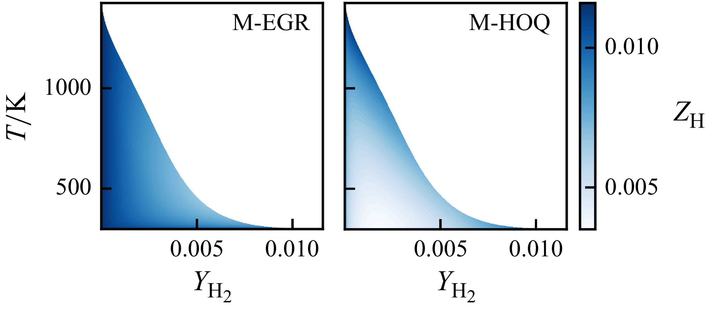


 Open access