

Introduction
In the Great Lakes region of the United States and Canada, pollen data derived from lacustrine and peatland sediments represent the most widely used proxy for the reconstruction of Late Quaternary paleoenvironments and paleoclimate conditions (e.g., Bernabo, Reference Bernabo1981; Anderson, Reference Anderson1995; Davis et al., Reference Davis, Douglas, Calcote, Cole, Winkler and Flakne2000; Yu, Reference Yu2000; Marlon et al., Reference Marlon, Pederson, Nolan, Goring, Shuman, Robertson and Booth2017; Watson et al., Reference Watson, Williams, Russell, Jackson, Shane and Lowell2018; Fastovich et al., Reference Fastovich, Russell, Jackson and Williams2020; Jensen et al., Reference Jensen, Fastovich, Watson, Gill, Jackson, Russell and Bevington2021). From these and other studies, researchers have identified prominent changes in the species composition of Holocene (11,700 cal yr BP to present) vegetation communities of the upper Great Lakes region resulting from changes in the abundance and geographic distribution of multiple arboreal pollen (AP) taxa (Davis et al., Reference Davis, Woods, Webb and Futyma1986; Bennett, Reference Bennett1988; Woods and Davis, Reference Woods and Davis1989; Brugam et al., Reference Brugam, Giorgi, Sesvold, Johnson and Almos1997; Jackson and Booth, Reference Jackson and Booth2002; Parshall, Reference Parshall2002). The paleoecological dynamics of the region’s major Holocene pollen taxa have been attributed to multiple biotic and abiotic factors, including postglacial migration and recolonization (Fuller, Reference Fuller1998), ecophysiological limitations on dispersal, pathogen outbreaks (Zhao et al., Reference Zhao, Yu and Zhao2010), climate change (Davis et al., Reference Davis, Douglas, Calcote, Cole, Winkler and Flakne2000; Hupy and Yansa, Reference Hupy, Yansa, Schaetzl, Darden and Brandt2009a, 2009b; Jackson et al., Reference Jackson, Booth, Reeves, Andersen, Minckley and Jones2014), pedogenic development and substrate constraints (Brubaker, Reference Brubaker1975; Graumlich and Davis, Reference Graumlich and Davis1993), and Indigenous land-use practices (Gajewski et al., Reference Gajewski, Kriesche, Chaput, Kulik and Schmidt2019).
Complementing vegetation-oriented palynological studies, other investigations have utilized testate amoebae to calibrate water-table fluctuations in regional lakes and peatlands, revealing substantial hydroclimatic variability occurring at decadal, centennial, and millennial timescales (Booth and Jackson, Reference Booth and Jackson2003; Booth, Reference Booth2010; Ireland et al., Reference Ireland, Booth, Hotchkiss and Schmitz2012). As a result of these multiple lines of proxy evidence, centennial- and millennial-scale Holocene hydroclimate variability has increasingly been implicated as an important modulator of regional lake and peatland hydrology and long-term patterns of vegetation change in the upper Great Lakes. Linkages have been suggested between modern forest species composition and regional Great Lakes climate phenomena such as lake-effect snowfall (LES; Henne et al., Reference Henne, Hu and Cleland2007; Fulton and Yansa, Reference Fulton and Yansa2021), lake-breeze cooling (Harman, Reference Harman1970), and enhanced moisture availability (Dodge, Reference Dodge1995). Similar climatological influences have also been inferred from the pollen record for prior millennia (Delcourt et al., Reference Delcourt, Nester, Delcourt, Mora and Orvis2002; Byun et al., Reference Byun, Cowling and Finkelstein2022). Climate changes that drove Holocene vegetation dynamics may have also modulated long-term Holocene water levels within the upper Great Lakes (Anderton and Loope, Reference Anderton and Loope1995; Lichter, Reference Lichter1995; Thompson and Baedke, Reference Thompson and Baedeke1997; Arbogast and Loope, Reference Arbogast and Loope1999; Baedke and Thompson, Reference Baedke and Thompson2000; Baedke et al., Reference Baedke, Thompson, Johnston and Wilcox2004; Thompson et al., Reference Thompson, Baedeke and Johnston2004; Lewis et al., Reference Lewis, King, Blasco, Brooks, Coakley, Croley and Dettman2008; Thompson et al., Reference Thompson, Lepper, Endres, Johnston, Baedke, Argyilan, Booth and Wilcox2011), as recent decades of lake-level fluctuations have been linked to precipitation variability (Hanrahan et al., Reference Hanrahan, Kravtsov and Roebber2010). Although aspects of the distinctive climatology of the Great Lakes region (Leighly, Reference Leighly1941; Kopec, Reference Kopec1965; Scott and Huff, Reference Scott and Huff1996; Hinkel and Nelson, Reference Hinkel and Nelson2012; Winkler et al., Reference Winkler, Burnett and Guentchev2022) have likely been active since the late Pleistocene (Griggs et al., Reference Griggs, Lewis and Kristovich2022), their temporal development, geographic extent, and overall impact on key environmental parameters such as vegetation composition and landscape stability remain largely unquantified, as does the overall sensitivity of the Great Lakes region to hydroclimate forcing (e.g., Salonen et al., Reference Salonen, Schenk, Williams, Shuman, Dauner, Wagner, Jungclau, Zhang and Luoto2025).
To this end, we generated a multiproxy record from Pup Lake, a small kettle basin in northern Lower Michigan, USA, with a particular focus on two potentially critical proxies: (1) magnetic susceptibility (MS) measurements of lake sediments and (2) detailed spatiotemporal analysis of Tsuga (hemlock) pollen at local (Pup Lake) and regional (Lower Michigan) scales. MS represents the acquired magnetization of a sediment sample when subjected to a low-frequency magnetic field, with the magnetizability of a sediment proportional to its concentration of magnetic minerals, chiefly iron oxides (Oldfield et al., Reference Oldfield, Barnosky, Loepold and Smith1983; Thompson and Oldfield, Reference Thompson and Oldfield1986; Gale and Hoare, Reference Gale and Hoare1992). Such minerals have both authigenic (within-basin; e.g., magnetotactic bacteria) and allogenic (extra-basinal; e.g., detrital, atmospheric fallout) sources (Dearing Reference Dearing1999a; Liu et al., Reference Liu, Roberts, Larrasoaña, Banerjee, Guyodo, Tauxe and Oldfield2012). A number of studies have postulated a functional relationship between lacustrine MS signals and hydroclimate, hypothesized to be mediated through precipitation and runoff (Rosenbaum et al., Reference Rosenbaum, Reynolds, Adam, Drexler, Sarna-Wojcicki and Whitney1996; Kodama et al., Reference Kodama, Lyons, Siver and Lott1997), lake-level fluctuations (Geiss et al., Reference Geiss, Umbanhowar, Camill and Banerjee2003; Li et al., Reference Li, Yu and Kodama2007), or groundwater flow/recharge (Maxbauer et al., Reference Maxbauer, Shapley, Geiss and Ito2020) and their impacts on erosion of catchment-wide and lake-marginal sediments. Interpreting lake-sediment MS chronologies as a function of paleoclimate requires (1) the development of a process-based conceptual model linking MS to climate change and (2) the use of a comparative multiproxy approach that enables direct evaluation of magnetic and independent nonmagnetic proxy records (Geiss et al., Reference Geiss, Umbanhowar, Camill and Banerjee2003) such as pollen. In particular, pollen taxa sensitive to variations in effective moisture would be best suited to such a goal. Tsuga canadensis (eastern hemlock) is a drought- and fire-intolerant coniferous tree species common throughout much of northern Lower Michigan and the Great Lakes region (Dickmann, Reference Dickmann2004; Kershaw, Reference Kershaw2006; Albert and Comer, Reference Albert and Comer2008; Voss and Reznicek, Reference Voss and Reznicek2012; Cohen et al., Reference Cohen, Kost, Slaughter and Albert2015) and has been an integral component of cool-mesic forests in the Great Lakes region and in northeastern North America for much of the Holocene (Foster, Reference Foster2014). Owing to its thin bark, shallow rooting system, and heavy litter deposits, Tsuga canadensis is generally regarded as one of the most drought-sensitive tree species within its range (Godman and Lancaster, Reference Godman, Lancaster, Burns and Honkala1990). As the establishment of Tsuga canadensis seedlings is inhibited by soil moisture stress (Carey, Reference Carey1993; Goerlich and Nyland, Reference Goerlich, Nyland, McManus, Shields and Souto2000; Rogers, Reference Rogers1978), local and regional hydroclimate conditions—and their interactions with soil texture—have likely influenced Tsuga’s geographic distribution and abundance during the Holocene. Variations in Tsuga pollen frequencies in regional pollen spectra have been noted during hydroclimate transitions (e.g., Booth and Jackson, Reference Booth and Jackson2002; Booth et al., Reference Booth, Notaro, Jackson and Kutzbach2006, Reference Booth, Jackson, Sousa, Sullivan, Minckley and Clifford2012b), and we seek to test and potentially extend the taxon’s utility as a sensitive paleoenvironmental indicator of key changes in Holocene hydroclimate conditions when utilized in conjunction with proxy records of MS and sedimentation rates from Pup Lake. Further, we compare our Pup Lake proxies to optically stimulated luminescence (OSL) dates from inland sand dunes across the Great Lakes region in order to assess whether Pup Lake’s history mirrors patterns of aeolian activity, erosion, and vegetation change that were potentially tied to regional-scale climate changes. Finally, we deploy a spatiotemporal analysis of existing regional Tsuga pollen profiles from multiple lacustrine and peatland sites in order to track changes in the taxon’s range that could shed light on broader questions of climate–vegetation–landscape interactions in the upper Great Lakes region during the Holocene, particularly the influence of the region’s distinctive lake-effect climatology (Eichenlaub, Reference Eichenlaub1970; Henne and Hu, Reference Henne and Hu2010; Henne et al., Reference Henne, Hu and Cleland2007).
Study area
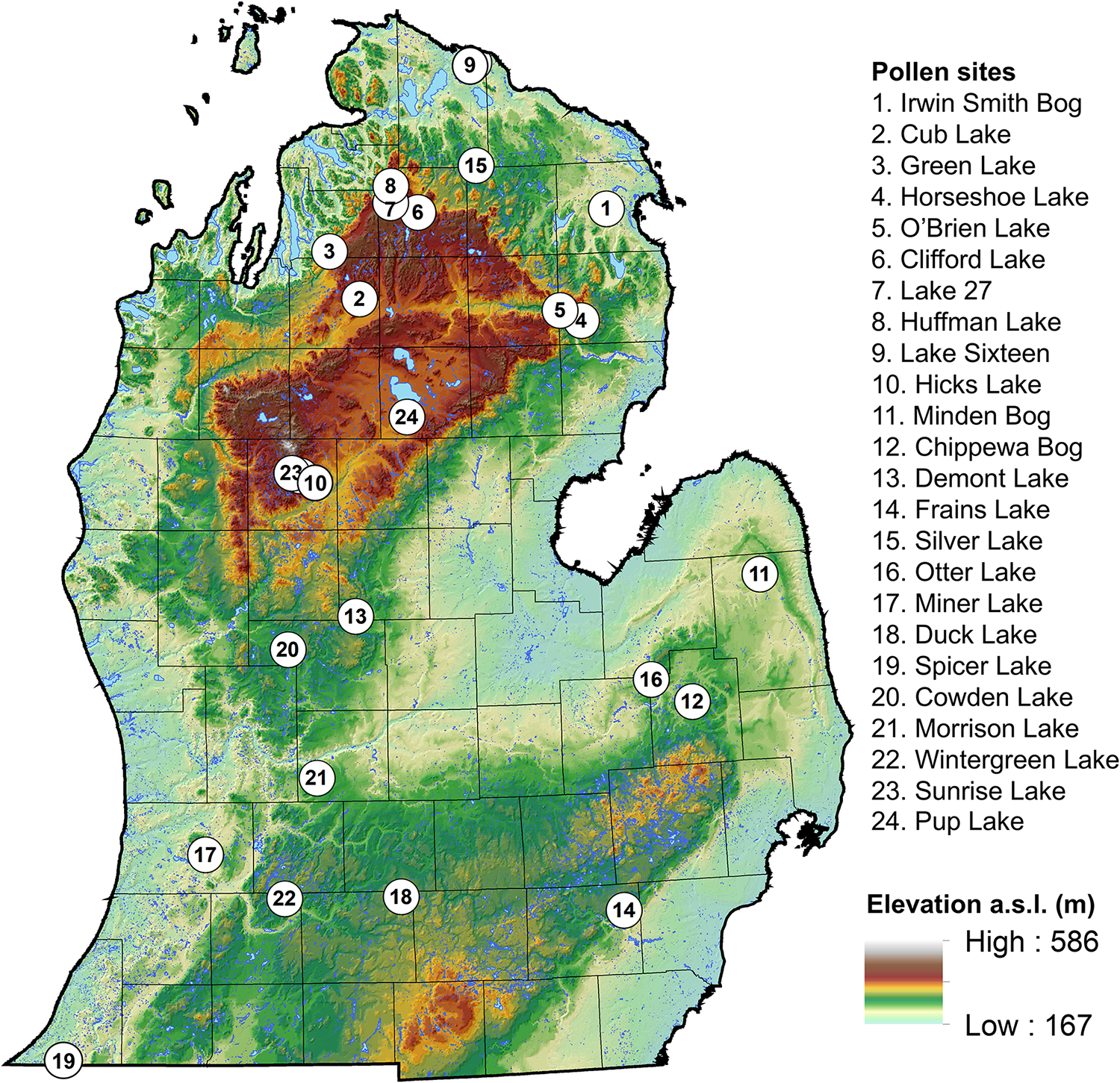
Pup Lake is a small (∼5.6 ha), deep (9.8 m) kettle lake at an elevation of 343 m above sea level in Roscommon County, MI, USA (44.24°N, 84.71°W; Fig. 1). The lake possesses a small inlet and outlet stream but is largely fed by underground springs. The topography is level to rolling and is underlain by deposits of coarse-textured, glacially derived outwash. High ridges of stratified ice-contact sand and gravel occur within ∼1–2 km of the lake. The east side of the lake features a prominent shoreline of a large paleolake, glacial Lake Roscommon, at 344.5 m (Schaetzl et al., Reference Schaetzl, Arbogast, Baish, Curry, Esch, Fulton II and Kincare2023). Upland soils are somewhat excessively drained or excessively drained sands and sandy loams, with poorly drained organic and mineral soils in lowland areas and depressions (Supplementary Fig. S1). Historic vegetation communities growing near Pup Lake were characterized by a mosaic of mesic (Fagus grandifolia [beech]–Acer saccharum [sugar maple]–Tsuga canadensis [eastern hemlock]), dry-mesic (Pinus strobus [white pine]–Pinus resinosa [red pine]–Quercus spp. [oak]), and dry (Pinus banksiana [jack pine]–Pinus resinosa-Quercus ellipsoidalis [northern pin oak]) northern forests, Pinus banksiana and Pinus banksiana–Quercus ellipsoidalis barrens, and extensive mixed conifer swamps of Abies balsamea (balsam fir), Larix laricina (tamarack), Picea mariana (black spruce), and Thuja occidentalis (northern whitecedar) in lowland areas (Cohen et al., Reference Cohen, Kost, Slaughter and Albert2015; Supplementary Fig. S2).
Study area location. (a) Michigan, USA (red shading) with respect to North America. (b) Lower and Upper Michigan within the wider Laurentian Great Lakes region. Pup Lake is indicated by the star. (c) Aerial view of Pup Lake looking south. (d) Bathymetric map of Pup Lake with coring location indicated.

The contemporary climate of the study area is cool humid-continental, with a mean January temperature of −7.4°C, a mean July temperature of 19.8°C, mean annual precipitation of ∼730 mm/yr, and mean annual snowfall of ∼1650 mm/yr (Houghton Lake National Weather Service station data, 1980–2009 climate normals; Garoogian, Reference Garoogian2011). Pup Lake’s interior position between Lakes Michigan (∼125 km to the west) and Huron (∼90 km to the east) attenuates the moderating influence of the Great Lakes on the area’s temperature and precipitation regimes. Thus, daily and yearly temperature ranges are larger, especially in summer, and temperature extremes are greater than in areas nearer to the Great Lakes’ shoreline. LES, primarily from Lake Michigan, tends to be heavier to the northwest of Pup Lake, progressively decreasing toward the south and east (Muller, Reference Muller1966; Eichenlaub, Reference Eichenlaub1970; Braham and Dungey, Reference Braham and Dungey1984; Norton and Bolsenga, Reference Norton and Bolsenga1993).
Methods
Field methods
Three sediment cores (A, B, and C; each separated by ∼0.5 m lateral distance) were taken from Pup Lake in the winter of 2019. The ice-platform surface overlaid an 865-cm-deep water column. Coring was done using a modified Livingstone piston corer and coring tower. Core A captured the sediment column from 878 cm to 1384 cm below the ice surface. Sediment recovery was not possible below 1384 cm, as sediments consisted of loose, coarse sand. Core B was taken at a depth offset of 50 cm with respect to core A. Core C was a duplicate recovery of only the bottommost 1 m of sediment. Visual correlation of basal laminations was used to align the three cores. The composite/duplicate core sediment was analyzed for pollen and plant macrofossils, and where possible, organic fragments were radiocarbon dated (see “Results”). Cores were wrapped in plastic film and placed inside halved PVC tubing for transfer to the Pollen Analysis Laboratory, Michigan State University. Cores were stored at 4.5°C before laboratory analyses.
Laboratory methods
To develop a radiocarbon chronology for the core, sediment samples of ∼20 cm3 volume (n = 123) were extracted from the core, sieved, and examined for plant macrofossils following the guidelines of Birks and Birks (Reference Birks and Birks1980). We used visual logging of core lithology, MS maxima and minima, and relative depth within lithostratigraphic units as a basis for guiding macrofossil extraction. Table 1 lists the Holocene-age radiocarbon samples from the Pup A core (n = 12), 10 of which provided results suitable for establishing chronological control. All radiocarbon dates were calibrated and the core’s age–depth model developed using the IntCal20 calibration curve (Reimer et al., Reference Reimer, Austin, Bard, Bayliss, Blackwell, Ramsey and Butzin2020) of the rbacon v. 2.4.3 package (Blaauw and Christen, Reference Blaauw and Christen2011) within the RStudio 2023.06.1 programming environment (RStudio Team, 2023). We present herein only median calibrated ages, determined at 2σ. Sedimentation rates (cm/yr) calculated using the core’s Holocene age–depth model were utilized in conjunction with pollen and MS data to track basin- and landscape-scale paleoenvironmental change.
Holocene-age radiocarbon dates (n = 12) from Pup Lake, northern Lower Michigan, USA: Core A.

* aRejected; too old for stratigraphic position.
† bRejected; too young for stratigraphic position.
Additional sediment samples (n = 119) were analyzed for pollen at variable depth increments ranging from 1 to 16 cm depending upon lithologic changes, radiocarbon age estimates, and inferred sedimentation rates derived from the core’s age–depth model. In general, the uppermost 100 cm of the core was sampled at a lower resolution (7 to 16 cm) due to higher sedimentation rates (cores A and C). Pollen samples were prepared according to standard chemical procedures (Faegri and Iverson, Reference Faegri, Iversen, Faegri, Kaland and Krzywinski1989). Pollen concentrates were examined at 400× magnification using a compound microscope and a minimum of 300 pollen grains of upland arboreal and herbaceous taxa (excluding Cyperaceae [sedge]) was counted per sample and identified to the greatest taxonomic resolution using a published key (McAndrews et al., Reference McAndrews, Berti and Norris1973) and the modern pollen reference collection in the Pollen Analysis Laboratory, Michigan State University. A few samples with low pollen abundances produced pollen counts <300 grains/sample. Pollen percentage data were plotted using Tilia 1.7.16 software (Grimm, Reference Grimm2019), and a constrained incremental sum-of-squares (CONISS) clustering algorithm was used to establish pollen zones. Vegetation community type descriptions, ecological characteristics, and plant geographic distributions used in this paper are based on data in Dickmann (Reference Dickmann2004), Voss and Reznicek (Reference Voss and Reznicek2012), and Cohen et al. (Reference Cohen, Kost, Slaughter and Albert2015), unless otherwise noted. Botanical terminology follows Barnes and Wagner (Reference Barnes and Wagner2004).
Whole-core volume MS (κ) analysis was performed to determine variations in the concentration of magnetic minerals present in the Pup Lake core (Dearing, Reference Dearing1999a; Gale and Hoare, Reference Gale and Hoare1992; Maher and Thompson, Reference Maher and Thompson1999; Thompson et al., Reference Thompson, Battarbee, O’Sullivan and Oldfield1975). Down-core variability in MS was used to infer the relative contribution of high-susceptibility allogenic sediments eroded from within the Pup Lake catchment into the lake’s basin (Dearing, Reference Dearing, Maher and Thompson1999b; Hatfield and Stoner, Reference Hatfield, Stoner and Elias2013; Liu et al., Reference Liu, Roberts, Larrasoaña, Banerjee, Guyodo, Tauxe and Oldfield2012; Oldfield, Reference Oldfield2013). We work from the assumption that long-term patterns of moisture variability in forested, humid-temperate regions directly affect soil erosion dynamics within a lake catchment by modulating two potential sources of detrital terrigenous magnetic minerals: (1) precipitation-mediated runoff, which contributes to erosional sediment flux (Jones et al., Reference Jones, Reinhardt, Dearing, Crook, Chiverrell, Welsh and Vergès2013; Kirby et al., Reference Kirby, Poulsen, Lund, Patterson, Reidy and Hammond2004; Kodama et al., Reference Kodama, Lyons, Siver and Lott1997; Thompson et al., Reference Thompson, Battarbee, O’Sullivan and Oldfield1975); and (2) lake-level fluctuations that expose, weather, and redeposit littoral-zone sediments (Li et al., Reference Li, Yu, Kodama and Moeller2006, Reference Henne, Hu and Cleland2007). Sediment cores were removed from refrigeration and allowed to stabilize to a temperature of 20°C before MS analysis. Measurements were made in triplicate at 1 cm intervals using a Bartington MS2F probe sensor and MS2 magnetic susceptibility meter with a low-frequency (0.465 kHz) applied magnetic field, with values recorded in dimensionless SI units. Individual MS readings were corrected for sensor drift, and triplicate values were averaged to yield a single mean measurement for each stratigraphic interval.
Statistical and comparative proxy analyses
Pup Lake pollen data were analyzed using nonmetric multidimensional scaling (NMS; Kent, Reference Kent2012) to ordinate pollen taxa and pollen sampling units along major paleoenvironmental gradients. For the NMS analysis, we utilized a similarity matrix of Pearson product-moment correlation coefficients of Hellinger (square-root)-transformed pollen data comprising stratigraphic samples (n = 96) and their associated pollen taxa (n = 22) in PC-ORD 6.19 (autopilot mode; medium speed and thoroughness; 2–4 axes; 50 runs on real data, 50 runs on randomized data; stability criterion = 0.00001; solution stability evaluation = 10 out of 200 maximum iterations; random starting coordinates; step length = 0.2; varimax rotation enabled; McCune and Mefford, Reference McCune and Mefford2011). Hellinger transformation of the raw pollen count data was deemed necessary before NMS analysis in order to down-weight the biasing influence of overly abundant taxa (Legendre and Gallagher, Reference Legendre and Gallagher2001) in the Pup Lake pollen record, particularly Pinus. NMS employs rank-order information within a multivariate (dis)similarity matrix between taxa and sampling units to reduce data dimensionality to a smaller number of synthetic axes (k-space) in which distances between taxa and sampling units have the same rank order as in the original (dis)similarity matrix (Kent, Reference Kent2012). Goodness of fit between rank orders in the k-space ordination and the (dis)similarity matrix is determined through a stress value ranging from 0 to 100, with values <20 generally indicating a robust ordination (Clarke, Reference Clarke1993). Once an initial solution was determined, NMS ordination was repeated four times using starting coordinates derived from the best solution of each run to verify the consistency of outputs across multiple runs. We generated plots of NMS scores for pollen taxa (to reconstruct paleoenvironmental gradients modulating forest composition dynamics) and stratigraphic sampling units (to track up-core temporal changes in paleoenvironmental gradients). We estimated the proportion of the total variance in the Pup Lake pollen data explained by each NMS axis by calculating coefficients of determination (r 2) between the relative Euclidean distance in the original, unreduced species space and Euclidean distance in the NMS ordination space (Peck, Reference Peck2010).
Pup Lake MS data were partitioned into discrete temporal zones using a customized script written in the R programming language (v. 4.4.2; R Core Team, 2024) utilizing the onlineBcp package (Yiğiter et al., Reference Yiğiter, Chen, An and Danacioglu2022). The onlineBcp algorithm implements Bayesian change point analysis methods to partition a univariate data sequence into segments by generating a posterior probability representing the likelihood of a change point occurring at each location within the sequence (Yiğiter et al., Reference Yiğiter, Chen, An and Danacioglu2015). For our analysis, we set theta (θ; probability of occurrence of a change point) to 0.1 and alpha (α) and beta (β)—hyperparameters of posterior distribution—to the default value of 1.0, with a threshold level for the posterior distribution of a change point set to 0.5. To minimize the potential biasing effect of anomalously high or low MS values on the detection of change points, we filtered the MS dataset for outliers using Grubbs’s test in the R package outliers (Komsta, Reference Komsta2022) before Bayesian change point analysis. We removed a total of six MS values identified as outliers based on initial G-test statistic results (MS outlier = 11.1 × 10⁻⁵ SI [1150 cm; 5016 cal yr BP]; G observed = 4.66; G critical = 3.36; P < 0.0001; α = 0.05) and computed z scores, which identified an additional five outlier MS values at 1252 cm (8176 cal yr BP), 1153 cm (5267 cal yr BP), 1152 cm (5183 cal yr BP), 1151 cm (5097 cal yr BP), and 1051 cm (2176 cal yr BP).
To evaluate regional spatiotemporal vegetation dynamics with respect to the Pup Lake pollen record, we obtained pollen data from multiple paleoecological sites (n = 23) across Lower Michigan, downloaded from the Neotoma Paleoecology Database website (https://www.neotomadb.org; Fig. 2, Table 2). Revised age–depth models for each site were constructed using the rbacon package (v. 3.3.1; Blaauw and Christen, Reference Blaauw and Christen2011; Blaauw et al., Reference Blaauw, Christen, Lopez, Vazquez, Gonzalez, Belding, Theiler, Gough and Karney2024) of the R programming language (v. 4.4.2; R Core Team, 2024) within the RStudio 2023.06.1 programming environment (RStudio Team, 2023) using each site’s available radiocarbon dates and the IntCal20 calibration curve (Reimer et al., Reference Reimer, Austin, Bard, Bayliss, Blackwell, Ramsey and Butzin2020). We specifically focused on temporal trends in Tsuga pollen across sites, due to the taxon’s drought and fire sensitivity (Goerlich and Nyland, Reference Goerlich, Nyland, McManus, Shields and Souto2000) and inferred relationship to LES gradients in northern Lower Michigan (Henne et al., Reference Henne, Hu and Cleland2007). Once revised age–depth models were created, we calculated the relative frequency of Tsuga pollen in each site’s pollen spectrum based on the sum of terrestrial AP and non-arboreal pollen (NAP) taxa for all dated stratigraphic intervals using the same taxa (n = 21) as identified in the Pup Lake core. The resulting data were linearly interpolated at 1000 year intervals using an R script (approx function) in order to (1) make direct inter-site comparisons at discrete points in time and (2) generate smoothed, continuous raster surfaces of regional Tsuga pollen frequencies using the Geostatistical Wizard tool of the Geostatistical Analyst toolbox (inverse distance weighting [IDW] algorithm; standard neighborhood type; minimum neighbors = 10; maximum neighbors = 15; sector type = 1 sector) in ArcGIS 10.8.2 (ESRI, 2021).
Location of Lower Michigan pollen sites (n = 24) used in the regional spatiotemporal analysis of Holocene Tsuga pollen dynamics. See Table 1 for site details.
Summary of pollen sites (n = 24) used in comparative spatiotemporal analysis of Holocene Tsuga pollen dynamics in Lower Michigan.
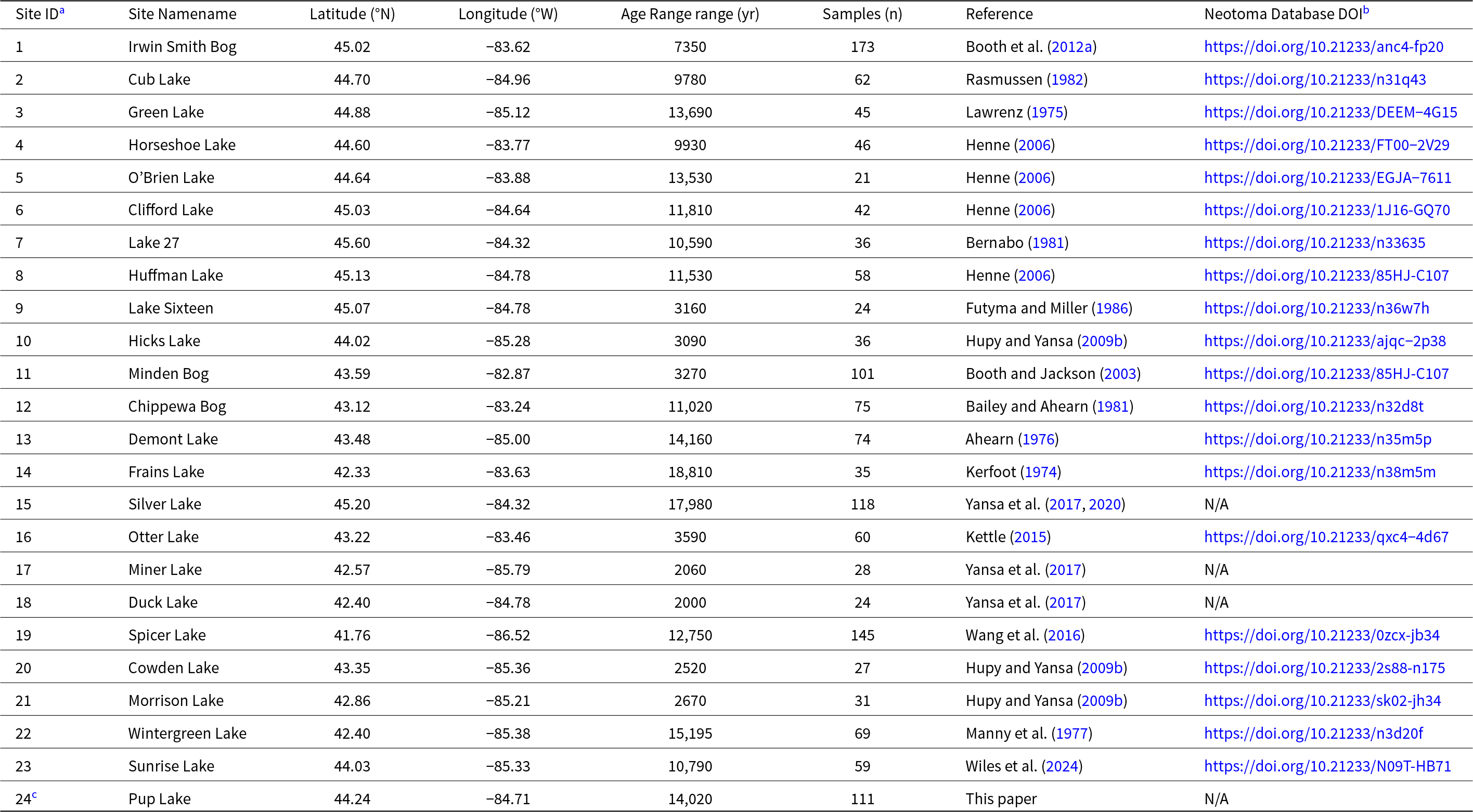
a See Fig. 2 for site locations.
b Twenty-three pollen profiles were downloaded from the Neotoma Paleoecology Database (https://www.neotomadb.org).
c up Lake data (Site ID 24) are from this paper.
To explore historic (post-1800 CE) Tsuga–LES associations within the Pup Lake study area, we created a raster dataset of mean annual snowfall totals for Lower Michigan interpolated from the 1981–2010 National Weather Service cooperative weather station data (Garoogian, Reference Garoogian2011) in ArcGIS 10.8.2 using the same IDW algorithm and settings utilized in the Tsuga pollen map interpolation stage described earlier. The interpolated raster was used to model the spatial relationship between snowfall totals and the distribution of eastern hemlock (Tsuga canadensis) witness trees within a 30 km buffer of Pup Lake during the umid-nineteenth century using georeferenced vegetation point data for Lower Michigan described in Paciorek et al. (Reference Paciorek, Cogbill, Peters, Williams, Mladenoff, Dawson and McLachlan2021) and downloaded from the EDI online data repository (https://portal.edirepository.org/nis/home.jsp; McLachlan, Reference McLachlan2020; McLachlan and Williams, Reference McLachlan and Williams2020a, Reference McLachlan and Williams2020b). Mean annual snowfall totals estimated at each eastern hemlock point feature were extracted using the Extract Values to Points tool of the ArcGIS Spatial Analyst toolbox. The total number of hemlock witness trees inside the 30 km buffer were tallied within each of six snowfall bins: ≤1499 mm/yr, 1500–1599 mm/yr, 1600–1699 mm/yr, 1700–1799 mm/yr, and ≥1800 mm/yr. To map snowfall, Tsuga canadensis witness trees, soils, and pre-Euro-American settlement vegetation patterns within the Pup Lake study area, we utilized a 30 km buffer surrounding the lake. This choice was based on calculations of the basin’s likely 90% pollen source area (estimated radius = 33.5 km) for light, buoyant pollen taxa with low fall speeds (mean grain diameter <32μm; e.g., Acer, Betula, Quercus, Salix) using the lake’s diameter (155 m) as a determinant of pollen source area (e.g., Sugita, Reference Sugita1993).
Because we (1) did not differentiate between the pollen of disturbance-adapted haploxylon (e.g., Pinus strobus) and fire-adapted diploxylon (e.g., Pinus banksiana and Pinus resinosa) pines during our analyses and (2) did not generate a charcoal record from Pup Lake’s sediments, we developed two pollen-based indices of moisture and disturbance regimes. First, we summed the percentage frequencies of all upland pollen taxa whose associated tree species are known to possess eco-physiological adaptations to xeric conditions and/or low-intensity surface fires (“pyrophilic taxa”; sum of Pinus, Quercus [oak], Carya [hickory], and Populus [aspen/poplar]; Thomas-Van Gundy and Nowacki, Reference Thomas-Van Gundy and Nowacki2013; Nowacki and Thomas-Van Gundy, Reference Nowacki and Thomas-Van Gundy2022). Upland pollen taxa associated with tree species favoring mesic conditions and/or fire intolerance were similarly tallied (“pyrophobic taxa”; sum of Acer [maple], Fagus [beech], Fraxinus [ash], Tsuga [hemlock], and Ulmus [elm]). We did not incorporate Betula (birch) into either the pyrophilic or pyrophobic taxa calculations, as the genus contains two species common in Lower Michigan with contrasting adaptations to moisture and fire, pyrophilic Betula papyrifera (paper birch) and pyrophobic Betula alleghaniensis (yellow birch) (Kershaw, Reference Kershaw2006). Second, we generated a vegetation disturbance index using the sum of all non-arboreal upland pollen taxa including Ambrosia (ragweed), Artemisia (mugwort), Poaceae (grasses), and other herb taxa unidentified to taxonomic group, divided by the sum of Acer, Fagus, and Tsuga pollen. We selected these taxa under the assumption that long-term, climatically modulated patterns of moisture variability would impact the relative frequencies of disturbance-adapted herbaceous taxa and late-successional, drought-intolerant Acer–Fagus–Tsuga communities (Cohen et al., Reference Cohen, Kost, Slaughter and Albert2015, while simultaneously minimizing the “swamping” effect of overrepresented Pinus pollen in the Pup Lake core.
Finally, we created a probability density plot (PDP) of the summed probability distribution (SPD) of OSL dates from inland sand dunes across the Great Lakes region (n = 177 dates) in order to evaluate relationships between dune activity and changing climate conditions inferred from the Pup Lake pollen, sedimentation rate, and MS records and regional Holocene Tsuga pollen trends. OSL data were compiled from the published literature (Arbogast et al., Reference Arbogast, Hansen and Van Oort2002a, Reference Arbogast, Wintle and Packman2002b, Reference Arbogast, Luehmann, Miller, Wernette, Adams, Waha and Oneil2015, Reference Arbogast, Luehmann, Monaghan, Lovis and Wang2017, Reference Arbogast, Lovis, McKeehan and Monaghan2023a; Arbogast and Packman, Reference Arbogast and Packman2004; Rawling et al., Reference Rawling, Hanson, Young and Attig2008; Loope et al., Reference Loope, Loope, Goble, Fisher, Jol and Seong2010, Reference Loope, Loope, Goble, Fisher, Lytle, Legg, Wysocki, Hanson and Young2012; Campbell et al., Reference Campbell, Fisher and Goble2011; Kilibarda and Blockland, Reference Kilibarda and Blockland2011; Vader et al., Reference Vader, Zeman, Schaetzl, Anderson, Walquist, Freiberger, Emmendorfer and Wang2012; Fisher et al., Reference Fisher, Blockland, Anderson, Krantz, Stierman and Goble2015, Reference Fisher, Horton, Lepper and Loope2019; Colgan et al., Reference Colgan, Amidon and Thurkettle2017). OSL dates for local sand dunes within the Pup Lake study area were obtained (Schaetzl, R.J., unpublished data). The kernel density estimate of OSL measurement values used in the SPD analysis was generated with an R script utilizing the Luminescence package (Kreutzer et al., Reference Kreutzer, Burow, Dietze, Fuchs, Schmidt, Fischer and Friedrich2025) employing default parameters, including Silverman’s rule of thumb for choosing the bandwidth of the kernel density estimator (Silverman, Reference Silverman1986).
Results
Chronology, stratigraphy, and pollen zonation
Ten radiocarbon dates were used to construct an age–depth model for the Pup Lake cores (Fig. 3). In general, sedimentation rates are highest at the top of the core (950–860 cm depth; 800 to −64 cal yr BP) and lowest between 1100 and 1200 cm depth, approximately dating to the Middle Holocene, 7000 to 3700 cal yr BP.
Pup Lake age–depth model for Holocene-age portion of Core A. (a) Markov chain Monte Carlo (MCMC) iterations. (b) Prior (green line) and posterior (shaded area) distributions of accumulation rate. (c) Prior (green line) and posterior (shaded area) distributions of memory (autocorrelation strength). (d) Age–depth model (shaded area). Node icons = age-estimate probability distributions; linear icons = user-input ages; stippled border = 95% confidence interval; red line = best-fit curve based on weighted mean ages. Uncalibrated 14C dates are also shown. Note that the x-axis represents depth below the Pup Lake ice surface (cm) during core extraction.

The core’s stratigraphy is characterized by several notable changes (Fig. 3). The basal portion of the Holocene-age sediments is composed of marl containing sapropelic gyttja rip-up clasts (1306–1269 cm; 9030–8480 cal yr BP). This basal unit is successively overlain by sapropelic gyttja (1269–1154 cm; 8480–4920 cal yr BP), sapropel (1154–872 cm; 8480–170 cal yr BP), and finally by a diffuse, organic-rich layer at the sediment–water interface (872–860 cm; 170–68 cal yr BP).
CONISS partitioning of the Pup Lake pollen data resulted in three primary zones (Fig. 4): (1) zone PL-1 (1278–1191 cm; 8770–6680 cal yr BP); (2) zone PL-2 (1191–1040 cm; 6680–2260 cal yr BP); and (3) zone PL-3 (1040–860 cm; 2260–68 cal yr BP). Details on the paleoenvironmental context and our interpretation of each zone and subzone are given in the following sections.
Pup Lake pollen diagram showing major pollen taxa (n = 21), percent pyrophilic (fire-tolerant) pollen taxa (sum of Pinus [pine], Quercus [oak], Carya [hickory], and Populus [aspen/poplar] pollen), percent pyrophobic (fire-intolerant) pollen taxa(sum of Tsuga [hemlock], Fagus [beech], Acer [maple], Fraxinus [ash], and Ulmus [elm]), Disturbance Index (ratio of all herbaceous pollen taxa to Fagus–Acer–Tsuga pollen), and sedimentation rate. Solid line above selected pollen taxa represents 5x exaggeration. Core lithostratigraphy, constrained incremental sum-of-squares (CONISS) dendrogram, and pollen zones are also shown.

Pollen zone PL-1 (1299–1186 cm; 9137–6460 cal yr BP)
The lowermost Holocene unit of the core, zone PL-1 is divided into three subzones (Fig. 4). PL-1a (1299–1292 cm; 9137–9002 cal yr BP; Pinus–Larix–Fraxinus–Cupressaceae), is the lowermost portion of a brecciated layer consisting of dark olive-gray (Munsell color: 5Y 3/2) marl matrix with black (5Y 2.5/2) sapropelic gyttja rip-up clasts approximately 0.5–1.5 cm in diameter. A radiocarbon date of 8055 ± 25 14C yr BP (2σ: 9030 to 8970 cal yr BP; 1298 cm; UCIAMS-230637) places this breccia unit within the Early Holocene (Table 1). This unit overlies a prominent late Pleistocene–age rhythmite layer (1385–1306 cm; not shown) of silty clay loam (dark grayish brown, 10YR 4/2 to light brownish gray, 10YR 6/2) with fine sand laminae (0.3 to 0.9 cm thickness; 10YR 6/2) and thin organic lenses. Below the rhythmites is an underlying coarse sand unit; the abrupt contact between these units represents an inferred depositional hiatus/unconformity across the Pleistocene–Holocene boundary, based on available radiocarbon dates (Schaetzl, R.J., unpublished data). Within this basal subzone, herbaceous pollen taxa including Poaceae (grasses; 5–8%), Ambrosia (ragweed; 5–6%), and Artemisia (mugwort; 2–4%) are found in relatively high frequencies (16–17% for combined NAP taxa) along with a variety of arboreal taxa, including moderate amounts of Pinus (17–25%), Larix (11–15%), Fraxinus (5–15%), and Cupressaceae (cedar/juniper, likely Thuja occidentalis; 2–14%). Tsuga pollen is entirely absent in subzone PL-1a. Sedimentation rates are also relatively high in this subzone, ranging from 0.05–0.14 cm/yr.
Overlying subzone PL-1b (1226–1246 cm; 9002–7612 cal yr BP; Pinus–Abies–Quercus–Ulmus–Picea) is dominated by Pinus (33–60%), with lesser amounts of numerous pollen taxa including Abies (fir; 7–16%), Larix (2–6%), Quercus (oak; 3–8 %), Cupressaceae (2–6%), Acer (maple; 1–4%), and Ulmus (3–5%). Minor quantities of Picea mariana (black spruce; 1–4%), Betula (birch; <1–3%), Fraxinus (<1–3%), Corylus (hazel; <1–4%), Populus (poplar/aspen; 1–3%), Salix (willow; ∼1%), and Carya (hickory; 0–3%) further characterize the pollen of this subzone. Tsuga pollen is absent or occurs in very low frequencies (0–1%).
Pollen subzone PL-1c (1246–1186 cm; 7612 to 6460 cal yr BP; Pinus–Abies–Ulmus–Quercus) is composed of black (5Y 2.5/2) sapropelic gyttja. A notable decline in Pinus pollen (60% at 7706 cal yr BP; 34% by 7152 cal yr BP) and a contemporaneous rise in Ulmus pollen (5% at 7612 cal yr BP; 11% by 7152 cal yr BP) is evident in this unit. Mesic upland pollen taxa are initially very low or absent, but begin rising, including Fagus (beech; 1% at 7494 cal yr BP; 5% by 6556 cal yr BP) and Tsuga (hemlock; <1% at 7379 cal yr BP; 5% by 6556 cal yr BP).
Pollen zone PL-2 (1186–1055 cm; 6460–2264 cal yr BP)
Pollen zone PL-2 encompasses the majority of the Mid-Holocene and the first half of the Late Holocene and is divided into three subzones (Fig. 4). PL-2a (1186–1151 cm; 6460 to 5097 cal yr BP; Pinus–Tsuga–Quercus–Ulmus–Fagus) is marked by a notable rise in Tsuga (4% at 6460 cal yr BP; 11% by 5404 cal yr BP) and Acer (2% at 6460 cal yr BP; 6% by 5267 cal yr BP). Quercus pollen also increases from 2% at 6326 cal yr BP to 10% by 5516 cal yr BP and Fagus (beech) pollen is variable, ranging from 2% to 7%. Subzone PL-2b (1151–1106 cm; 5097–3725 cal yr BP; Pinus–Fagus–Acer) is notable for the prominent decline in Tsuga pollen commencing during terminal PL-2a (11% at 5404 cal yr BP; 2% by 4918 cal yr BP). A variety of hardwood and coniferous taxa show modest increases during the Tsuga decline, including Fagus (4% at 5097 cal yr BP; 11% by 4908 cal yr BP), Acer (3% at 4918 cal yr BP; 7% by 4627 cal yr BP), Betula (2% at 5016 cal yr BP; 4% by 4438 cal yr BP), Pinus (38% at 5016 cal yr BP; 45% by 4250 cal yr BP), Cupressaceae (4% at 5097 cal yr BP; 7% by 4908 cal yr BP), and Larix (4% at 5097 cal yr BP; 6% by 4817 cal yr BP). Sedimentation rates are the lowest of the entire Holocene during the Tsuga decline, averaging ∼0.01 cm/yr. During final subzone PL-2c (1106–1055 cm; 3725 to 2264 cal yr BP; Pinus–Tsuga–Betula), the most notable change is the progressive increase in Tsuga pollen (3% at 3827 cal yr BP; 11% by 2641 cal yr BP) and the simultaneous decline of Pinus (42% at 3412 cal yr BP; 22% by 2461 cal yr BP). Sedimentation rates increase slightly from subzone PL-2b, averaging ∼0.03 cm/yr.
Pollen zone PL-3 (1055–852 cm; 2264 to −64 cal yr BP)
The uppermost pollen zone of the Pup Lake record is divided into three subzones (Fig. 4). Subzone PL-3a (1055–974 cm; 2264–886 cal yr BP; Pinus–Tsuga–Fagus), is characterized by a continued increase in Tsuga pollen that began during subzone PL-2c, culminating in a Holocene peak frequency of 30% by 1578 cal yr BP. Fagus percentages also rise slightly during subzone PL-3a, from 6% at 2087 cal yr BP to 11% by 1938 cal yr BP, while Pinus pollen is variable (20% at 1938 cal yr BP; 51% at 802 cal yr BP). Subzone PL-3b (974–910 cm; 886 to 216 cal yr BP; Pinus–Abies–Poaceae) exhibits a steady decline in Pinus from 51% at the top of the subzone to 31% by 300 cal yr BP. This is accompanied by decreasing Tsuga values (16% at 984 cal yr BP; 4% by 802 cal yr BP) and an increase in Poaceae pollen (2% at 886 cal yr BP; 6% by 356 cal yr BP). Abies (9% at 802 cal yr BP; 15% by 550 cal yr BP) and Picea mariana (0% at 802 cal yr BP; 4% by 550 cal yr BP) both increase during subzone PL-2b. Final subzone PL-3c (910–852 cm; 216 to −64 cal yr BP; Pinus–Ambrosia) possesses pollen signatures suggesting disturbance such as forest clearance and agricultural activity related to Euro-American settlement. For example, Ambrosia, which rarely exceeds 1% for most of Pup Lake’s Holocene pollen record, increases to 7% by 81 cal yr BP. Overall, sedimentation rates rise progressively during the entirety of pollen zone PL-3 (range = 0.04–0.3 cm/yr; 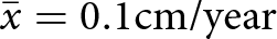 $\bar{x} = 0.1 {\text{cm/year}}$; s = 0.07 cm/yr), with peak levels typical of the Early Holocene evident within Euro-American subzone PL-3c.
In general, xeric pyrophilic pollen taxa—chiefly Pinus—tend to decrease slightly over the course of the Holocene, while mesic pyrophobic taxa increase (Fig. 4). The major exception to this trend occurs after 1000 cal yr BP, where there is an evident rise in pyrophilic taxa and coeval decrease in pyrophobic pollen taxa. The disturbance index declines sharply from 9100 to 8900 cal yr BP, with a slight increase at ∼8100 cal yr BP. Values then decline to low levels until another minor increase appears between 5000 and 4000 cal yr BP, followed by a gradual decline. After 1000 cal yr BP, the disturbance index increases again, with a final rise beginning at ∼200 cal yr BP.
NMS ordination and paleoenvironmental gradients
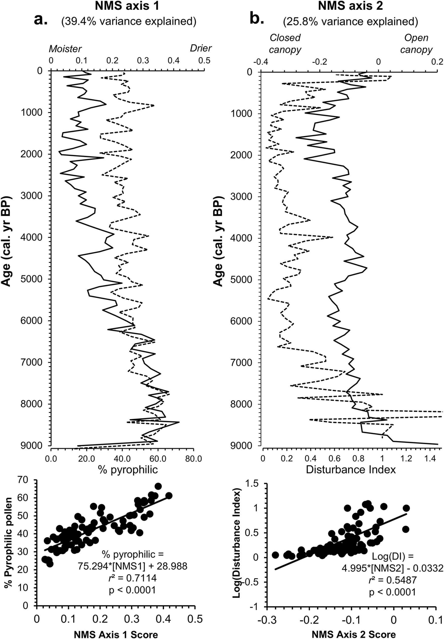
NMS ordination of Pup Lake’s Holocene pollen spectrum resulted in a solution (final stress = 7.63) possessing two primary axes collectively explaining 65.2% of the total variance in the pollen data (Fig. 5). NMS axis 1 (39.4% variance explained; Fig. 5a) is very strongly positively correlated with percent pyrophilic pollen taxa (r = 0.8184; P < 0.0001) and is interpreted as a gradient in moisture availability and/or fire frequency/intensity. NMS axis 2 (25.8% variance explained; Fig. 4) is strongly positively correlated with percent NAP and is interpreted as a gradient in vegetation disturbance and/or forest canopy density.
Chronology of nonmetric multidimensional scaling (NMS) scores (top; solid lines) generated from the full Pup Lake Holocene pollen spectrum, compared with inferred paleoenvironmental correlates (dashed lines). Correlation scatter plots of NMS scores and environmental correlates are shown at bottom. Collectively, NMS axes 1 and 2 explain 65.2% of the pollen data’s total variance. (a) NMS axis 1 (39.4% variance explained) is very strongly positively correlated with percent pyrophilic (i.e., fire- and drought-tolerant) pollen taxa and is interpreted as a gradient in moisture availability. (b) NMS axis 2 (25.8% variance explained) is strongly positively correlated with percent non-arboreal pollen (NAP) and is interpreted as a disturbance and/or canopy density indicator.
Scatter plots of NMS axis 1 and 2 scores (Fig. 6a) place major pyrophobic (fire/drought-intolerant) upland forest taxa, including Tsuga (hemlock), Fagus (beech), and Betula (birch) along the lower left portion of the axis, with pyrophilic (fire-/drought-tolerant) upland forest taxa such as Pinus (pine) and Quercus (oak) along the right side of the axis. Several herbaceous pollen taxa indicative of open or disturbed sites (e.g., Ambrosia, Artemisia, Poaceae) are positioned near the top of the graph. NMS plots of pollen sampling units (Fig. 6b) indicate a temporal shift away from open-land, herbaceous indicator taxa in the earliest Holocene samples (∼9100–9000 cal yr BP; “Start”) near the top of the ordination diagram toward pyrophilic Pinus and Quercus (9000–7000 cal yr BP) along the right, followed by a gradual transition during the Mid-Holocene toward the lower left-hand side of the diagram, associated with mesic Tsuga and Fagus. A slight shift toward herbaceous taxa near the top of the NMS plot is evident in the most recent samples (−64 cal yr BP; “End”).
Plot of nonmetric multidimensional scaling (NMS) axis 1 and 2 scores of major Pup Lake Holocene pollen taxa (circles) and pollen sampling units (crosses). NMS axis 1 (abscissa; 39.4% variance explained) is interpreted as a moisture-availability gradient, with mesic upland (e.g., Acer, Betula, Fagus, Tsuga) and lowland/wetland (e.g., Alnus, Corylus, Cupressaceae, Cyperaceae, Picea mariana) taxa grouped on the left side of the axis and pyrophilic upland forest taxa (e.g., Pinus, Quercus) on the right side. NMS axis 2 (ordinate; 25.8% variance explained) is interpreted as a disturbance and/or canopy density gradient, with several herbaceous open-land indicator taxa (e.g., Ambrosia, Artemisia, Poaceae) arranged near the top of the graph, with closed-canopy forest taxa at the bottom. In a, crosses represent pollen sampling units and their 2σ median calibrated radiocarbon dates shown with respect to major pollen taxa. (b) Detail of sampling units labeled with associated 2σ median calibrated radiocarbon dates. Dashed line indicates up-core temporal trajectory of NMS scores from oldest (9137 BP; “Start”) to youngest (−64 BP; “End”).

Holocene MS trends
The Pup Lake MS record exhibits high-magnitude (n = 6) peaks at 9250, 8130, 5240, 2480, 810, and 120 cal yr BP (Fig. 7). Additionally, several low-magnitude (n = 6) MS peaks are evident at 8700, 7000, 6200, 5900, 1900, and 290 cal yr BP. These short-term (centennial- to sub-centennial timescale) positive excursions are superimposed upon longer-term (multi-centennial- to millennial-scale) phases of elevated (n = 4; 9300–8100, 7200–5200, 3200–800, and 500–0 cal yr BP) and low/negative (n = 3; 8100–7200, 5200–3200, and 800–500 cal yr BP) MS values (Fig. 7). The onlineBcp algorithm identified three change points within the MS data: at 1248 cm (posterior probability = 0.77), 1148 cm (posterior probability = 0.78), and 1048 cm (posterior probability = 0.64). These change points define four temporal MS zones: zone 1 (1302–1249 cm; 9300–8110 BP; x̅ = 2.02 × 10⁻⁵ SI; s = 3.11; P = 0.0002), zone 2 (1248–1149 cm; 8110–5170 BP; x̅ = 0.98 × 10⁻⁵ SI; s = 1.84; P < 0.0001), zone 3 (1148–1049 cm; 5170–2440 BP; x̅ = 0.34 × 10⁻⁵ SI; s = 1.53; P < 0.0001), and zone 4 (1048–878 cm; 2440–120 BP; x̅ = 1.22 × 10⁻⁵ SI; s =2.09; P = <0.0001).
Holocene Pup Lake magnetic susceptibility (MS) record with major (i.e., >5.0 × 10⁻⁵ SI; n = 6) and minor (i.e., <5.0 × 10⁻⁵ SI; n = 6) peaks labeled with 2σ median calibrated radiocarbon dates. MS zonation determined using Bayesian change point analysis performed with the onlineBcp R package (Yiğiter et al., Reference Yiğiter, Chen, An and Danacioglu2015). Red dashed line represents 3× exaggeration of main MS curve (solid black line). The main curve has been truncated at 0.0 × 10⁻⁵ SI to better emphasize millennial-scale, high-MS phases. Major Tsuga pollen events at Pup Lake are shown in blue. Inferred moist (blue capital letter “M”; high-MS phases) and dry (red capital letter “D”; low-MS phases) conditions are indicated. Prominent paleoclimate episodes are labeled in black. DACP/LALIA, Dark Ages Cold Period/Late Antique Little Ice Age; MCA, Medieval Climate Anomaly (REFS); LIA, Little Ice Age.

Comparative proxy analyses
Pup Lake’s MS and Tsuga pollen records are broadly aligned with each other (Fig. 8a and b). A period of elevated MS values is evident after 7000 cal yr BP, continuing until ∼5000 BP, largely overlapping with (1) the Mid-Holocene Tsuga peak from 6800 to 5200 cal yr BP, (2) a slight increase in sedimentation rate followed by gradual decline (Fig. 8c), and (3) the latter portion of the Nipissing I high stand (Fig. 8d). A subsequent phase of decreasing MS values from ∼5200 to 3800 cal yr BP is accompanied by a coeval decline in Tsuga pollen, an increase in sedimentation rate, and the Nipissing II high stand. A progressive increase in MS values after 3800 cal yr BP is closely timed with the prolonged resurgence of Tsuga and the Algoma high stand. These trends culminate in notable increases in MS, Tsuga pollen, and sedimentation rate from 2100 to 1000 cal yr BP and an unnamed Lake Michigan high stand. These temporal patterns are further reflected in changing correlation patterns between Tsuga pollen frequencies, sedimentation rates, and MS at Pup Lake during the Holocene. Percent Tsuga pollen and sedimentation rates exhibit a strong, negative relationship (r = −0.72; P <0.0001) from 8200 to 5200 cal yr BP, which changes to a very strong, positive correlation (r = 0.88; P < 0.0001) from 5200 to 1000 cal yr BP (Fig. 8e). This relationship weakens and becomes statistically insignificant (r = 0.36; P = 0.39) from 1000 cal yr BP to the present. The relationship between MS and sedimentation rate also changes through time, from a medium, negative correlation (r = −0.38; P = 0.05) from 8200 to 5200 cal yr BP, to a strong, positive relationship (r = 0.64; P < 0.0001) from 5200 to 1000 cal yr BP, and a somewhat stronger, positive correlation (r = 0.73) that is marginally statistically insignificant (P = 0.06) after 1000 cal yr BP (Fig. 8f). Finally, the relationship between MS and percent Tsuga pollen demonstrates a moderate, positive correlation (r = 0.42; P = 0.03) from 8200 to 5200 BP, a strong, positive correlation (r = 0.64; P < 0.0001) from 5200 to 1000 cal yr BP, and a very weak, positive, correlation (r = 0.13) that is highly statistically insignificant (P = 0.79) after 1000 cal yr BP (Fig. 8g).
Comparison of Holocene temporal trends in: (a) Pup Lake magnetic susceptibility (MS; numbers indicate 2σ median calibrated dates for selected MS peaks; major paleoclimate events are also labeled); (b) Pup Lake Tsuga pollen frequencies; (c) Pup Lake sedimentation rate (purple dashed line denotes 3× exaggeration to better highlight temporal trends); (d) reconstructed Lake Michigan water levels (modified from Baedke and Thompson, Reference Baedke and Thompson2000; dashed portion of the line represents hypothesized water-level curve; question mark denotes unnamed Late Holocene high stand); (e) correlation between Tsuga pollen frequencies and sedimentation rate decomposed into three temporal intervals (8200–5200 cal yr BP; 5200–1000 cal yr BP; 1000–0 cal yr BP); (f) temporally decomposed correlation between MS and sedimentation rate; and (g) temporally decomposed correlation between MS and Tsuga pollen frequencies.

Great Lakes regional inland dune activity
SPD analysis of inland sand dune OSL ages reveals two phases of dune formation and stabilization: (1) during the late Pleistocene, generally between 13,500 and 12,500 yr ago, and (2) a larger phase, generally between 11,000 and 9000 yr ago (Fig. 9). The termination of the Early Holocene growth phase is closely followed by the arrival, establishment, and expansion of Tsuga both at Pup Lake and across Lower Michigan after 8000 cal yr BP.
Probability density plot (PDP) of published optically stimulated luminescence (OSL) ages (n = 177) from inland sand dunes in the Great Lakes region (blue solid line; data sources listed in text). Mean percent Tsuga pollen from Lower Michigan paleoecological sites (red solid line; n = 23 sites; Table 2) and Pup Lake Tsuga pollen percentages (solid purple line) are also shown. Dunes along the shorelines of the Great Lakes were not included in the OSL analysis because they may be primarily responding to lake-level fluctuations more than to paleoclimate drivers (Arbogast and Loope Reference Arbogast and Loope1999; Arbogast et al., Reference Arbogast, Hansen and Van Oort2002a, Reference Arbogast, Wintle and Packman2002b, Reference Arbogast and Packman2004). The rapid termination of the PDP peak after ca. 9000 yr ago generally coincides with the early phases of the re-establishment of lacustrine conditions at Pup Lake by 9100 cal yr BP. Before this time, Pup Lake may have been dry. Note that initial Mid-Holocene Tsuga establishment (after ∼8200 BP) and rise (after 6800 BP)—both regionally and at Pup Lake—also coincide with the attenuating PDP peak, suggesting increasingly mesic conditions across Lower Michigan.

Tsuga spatiotemporal dynamics
Tsuga spatiotemporal patterns indicate a shifting geographic distribution and major changes in the relative frequency of Tsuga during the Holocene (Fig. 10). At 9000 cal yr BP, Tsuga pollen was present in very low frequencies (<1%) in the extreme eastern part of Lower Michigan (Fig. 10a). By 8000 cal yr BP, frequencies were still very low; however, sites with the highest Tsuga pollen percentages had shifted inland away from Lake Huron to include Pup Lake (<1%; Fig. 10b). From 7000 to 6000 cal yr BP, Tsuga values were highest within the northeastern part of Lower Michigan, with near-peak values for the Mid-Holocene (12–24%) attained by 6000 cal yr BP (Fig. 10c and d), with Tsuga pollen rising from 1% (7000 cal yr BP) to 6% (6000 cal yr BP) at Pup Lake. This was followed by rapidly declining Tsuga percentages by 5000 cal yr BP (regional maximum = 13%; Pup Lake = 3%; Fig. 10e) and 4000 cal yr BP (regional maximum = 8%; Pup Lake = 3%; Fig. 10f). Notably, by 4000 cal yr BP, the area of maximum Tsuga percentages had shifted to northwestern Lower Michigan (Fig. 10f). Subsequently, from 3000 to 1000 BP, Tsuga pollen experienced a resurgence and major geographic expansion to the east and south (Fig. 10g–i), followed by a slight decline and marked retreat to the northwest over the last millennium (Fig. 10j).
Spatiotemporal dynamics of Tsuga pollen frequencies across Lower Michigan, 9000–0 BP, linearly interpolated at 1000 yr intervals from lacustrine and peatland pollen spectra (n = 23) downloaded from the Neotoma paleoecology database (https://www.neotomadb.org; see Table 2 and Figure 2) and Pup Lake pollen data (this paper). Tsuga percentages were calculated for each site using the same taxa (n = 21) as identified in the Pup Lake core. Green star indicates the location of Pup Lake. Note (a) initial presence of Tsuga pollen at very low frequencies (<1%) in extreme eastern Lower Michigan, associated with inferred Early Holocene Tsuga colonization (9000 BP); (b–c) range shift into north-central and northeastern Lower Michigan at continued low percentages (<2%; 8000–7000 BP); (d) major increase within northeastern core (6000 BP); (e) initial decline (5000 BP); (f) continued decline and northwestward shift (4000 BP); (g–i) recovery and subsequent expansion toward the south and east (3000–1000 BP); and (j) northwesterly retreat (0 BP).

Discussion
Our records of pollen, MS, and sedimentation rates from Pup Lake reveal notable covarying relationships among these proxies over the course of the Holocene, with an overall trend of increasing available moisture following the transition from the Early to the Middle Holocene. The regional dune OSL chronology conforms well with this interpretation, suggesting increasing effective moisture, both locally and regionally, as the Pup Lake basin infilled by ∼9000 cal yr BP following a prolonged period of non-deposition and erosion during the terminal Pleistocene and Early Holocene. The stabilization of regional aeolian systems after 9000 cal yr BP, as suggested by the probability density plot of OSL ages (Fig. 9), presumably occurred in response to ameliorating and more mesic climate conditions. This aligns with (1) the timing of Tsuga arrival at Pup Lake by 8200 cal yr BP and its subsequent rise after 6800 cal yr BP, culminating in its Mid-Holocene peak by 5400 cal yr BP, and (2) the sharp decline in the disturbance index between 9100 and 8900 cal yr BP (Fig. 4).
The Pup Lake proxy data further reveal distinct MS variations that appear to be associated with long-term patterns of Tsuga pollen variability at Pup Lake. For example, the initial arrival of Tsuga ca. 8200 cal yr BP is closely timed with a major MS peak at 8130 cal yr BP. The Mid-Holocene Tsuga rise beginning ∼6800 cal yr BP follows a minor MS peak at 7000 cal yr BP, and the subsequent Mid-Holocene Tsuga peak occurs during an extended phase of elevated MS values from 7400 to 5200 cal yr BP. The Mid-Holocene Tsuga decline—which occurs at ∼5200 cal yr BP at Pup Lake—is coeval with the termination of an MS peak at 5240 cal yr BP. The post-decline period of low Tsuga pollen from ∼5000 to 3800 cal yr BP falls within a phase of the lowest MS values of the entire Holocene at Pup Lake. The initial Late Holocene Tsuga rise beginning ∼3800 cal yr BP commences as MS values begin to increase steadily, coinciding with the Late Holocene Tsuga rise. An MS peak at 2480 cal yr BP occurs shortly before the commencement of the Late Holocene Tsuga peak at ∼2250 cal yr BP. Another major MS peak at 1900 cal yr BP precedes maximum Tsuga values of the entire Holocene at 1580 cal yr BP. The prominent decline in Tsuga percentages after this date accelerates in tandem with the onset of yet another major MS peak at 810 cal yr BP, an event noted as a significant, brief, wet episode at Minden Bog (Booth and Jackson, Reference Booth and Jackson2003) and Houghton and Higgins Bogs near Pup Lake (Sales, Reference Sales2017) and identified in numerous MS profiles from the lower Great Lakes region (Fulton, A.E., unpublished data). Tsuga percentages and MS values remain very low for a few centuries following the 810 cal yr BP MS peak, but both increase in tandem beginning ∼500 cal yrs BP. The proxies diverge after ∼200 cal yr BP, with MS values continuing to increase sharply, while Tsuga pollen percentages decline to the present time (Fig. 8).
To our knowledge, our study is the first to identify a relationship between Tsuga pollen frequencies and MS variations, contributing a novel insight to regional Holocene paleoecological research. The fact that many of Pup Lake’s high-magnitude positive MS peaks, including the earliest Holocene peak at 9250 cal yr BP and others at 8130, 5240, and 2480 cal yr BP, appear to be closely associated with major, widely recognized paleoclimate events at continental, hemispheric, and global spatial scales (e.g., Magny, Reference Magny2004; Helama et al., Reference Helama, Stoffel, Hall, Jones, Arppe, Matskovsky, Timonen, Nöjd, Mielikäinen and Oinonen2021) is noteworthy. Such events include the 9.2 ka BP event (Fleitmann et al., Reference Fleitmann, Mudelsee, Burns, Bradley, Kramers and Matter2008; Yu et al., Reference Yu, Colman, Lowell, Milne, Fisher, Breckenridge, Boyd and Teller2010; Flohr et al., Reference Flohr, Fleitmann, Matthews, Matthews and Black2016), 8.2 ka BP event (Alley and Ágústsdóttir, Reference Alley and Ágústsdóttir2005; Cheng et al., Reference Cheng, Fleitmann, Edwards, Wang, Cruz, Auler and Mangini2009), 5.2 ka BP event (Magny and Haas, Reference Magny and Hass2004; Roland et al., Reference Roland, Daley, Caseldine, Charman, Turney, Amesbury, Thompson and Woodley2015), 2.5 ka BP event (van Geel et al., Reference van Geel, Buurman and Waterbolk1996), and the Little Ice Age (LIA; Clifford and Booth Reference Clifford and Booth2015; Owens et al., Reference Owens, Lockwood, Hawkins, Usoskin, Jones, Barnard, Schurer and Fasullo2017). Other major paleoclimate events are variously associated with (1) prolonged, gradual increases in MS values (e.g., the 3.2 ka BP event; Drake Reference Drake2012), (2) sharp MS declines (e.g., the Medieval Climate Anomaly [MCA]; Mann et al., Reference Mann, Zhang, Rutherford, Bradley, Hughes, Shindell and Ammann2009; Diaz et al., Reference Diaz, Trigo, Hughes, Mann, Xoplaki and Barriopedro2011; Booth et al., Reference Booth, Jackson, Sousa, Sullivan, Minckley and Clifford2012b), and (3) ambiguous or non-evident MS trends such as the 4.2 ka BP event (Booth et al., Reference Booth, Jackson, Forman, Kutzbach, Bettis, Kreigs and Wright2005; McFadden et al., Reference McFadden, Mullins, Patterson and Anderson2004; Min and Liang, Reference Min and Liang2019), the Roman Warm Period (Lepofsky et al., Reference Lepofsky, Lertzman, Hallett and Mathewes2005; Booth et al., Reference Booth, Notaro, Jackson and Kutzbach2006), and the Dark Ages Cold Period/Late Antique Little Ice Age (DACP/LALIA; Helama et al., Reference Helama, Jones and Briffa2017).
The bracketing of the Mid-Holocene Tsuga peak at Pup Lake by major positive MS excursions at 8130 and 5240 cal yr BP suggests a potentially important role for the 8.2 and 5.2 ka BP events as triggers for changes in regional hydroclimate and forest composition, particularly as they relate to the initial Mid-Holocene rise and subsequent terminal decline of Tsuga throughout the Laurentian Great Lakes and Northeast regions (Allison et al., Reference Allison, Moeller and Davis1986; Boucherle et al., Reference Boucherle, Smol, Oliver, Brown and McNeely1986; Bhiry and Fillion, Reference Bhiry and Filion1996; Fuller, Reference Fuller1998; Bennett and Fuller, Reference Bennett and Fuller2002; Booth et al., Reference Booth, Brewer, Blaauw, Minckley and Jackson2012a). We also note that the MS peak at 8130 cal yr BP is accompanied by a slight, but evident, increase in the disturbance index, suggesting that climate changes were severe enough to impact local vegetation, if only marginally. Several paleoecological studies have postulated a connection between the Mid-Holocene Tsuga decline and increased regional aridity (e.g., Yu et al., Reference Yu, McAndrews and Eicher1997; Haas and McAndrews, Reference Haas, McAndrews, McManus, Shields and Souto2000; Calcote, Reference Calcote2003; Foster et al., Reference Foster, Oswald, Faison, Doughty and Hansen2006; Zhao et al., Reference Zhao, Yu and Zhao2010; Oswald and Foster, Reference Oswald and Foster2011; Marsicek et al., Reference Marsicek, Shuman, Brewer, Foster and Oswald2013), an interpretation supported by generally elevated but variable MS values before 5200 cal yr BP. The period following the Mid-Holocene Tsuga decline is characterized by low MS values and a minor increase in the disturbance index, indicating that conditions at Pup Lake were likely drier, with attenuated erosion and slightly more open-canopy forests (Fig. 4). The contemporaneous 4.2 ka BP event is noted as a period of severe drought in the upper Great Lakes region (Booth et al., Reference Booth, Jackson, Forman, Kutzbach, Bettis, Kreigs and Wright2005).
Our conceptual model linking MS to hydroclimate was based on the hypothesis that MS variations within the Pup Lake core were likely a reflection of centennial- and millennial-scale moisture dynamics due to either (1) precipitation-mediated runoff or (2) redeposition of littoral-zone sediments arising from lake-level fluctuations. As the landscape immediately surrounding Pup Lake possesses relatively limited topographic relief, we propose that the source of the lake’s MS signals derives from a two-step process: (1) subaerial exposure of lake sediments as water levels fall during periods of increasing aridity and (2) subsequent erosion and redeposition of sediments into deeper portions of the basin as lake levels rise during phases of increasing moisture availability. The densely forested environment surrounding Pup Lake during the Holocene likely inhibited the efficacy of runoff as an erosional mechanism, as has been suggested in other MS-based studies of lakes in humid-temperate regions (e.g., Li et al, Reference Li, Yu, Kodama and Moeller2006, Reference Li, Yu and Kodama2007). The overall good fit between our magnetic and independent, nonmagnetic proxies (pollen, sedimentation rates, OSL dates), combined with robust chronological control, suggests that the Pup Lake MS record has responded sensitively and consistently to both long-term local and regional patterns of climate change and that sediment records of MS (and other environmental magnetic parameters) from the region’s small lakes hold promise for future paleoclimate studies (e.g., Geiss et al., Reference Geiss, Umbanhowar, Camill and Banerjee2003).
In addition to the apparent relationship between MS and Tsuga pollen frequencies, the Pup Lake record also suggests connections between these proxies and the lake’s lithologic transitions. We note that the change from marl to sapropelic gyttja at 1249 cm coincides with the 8130 cal yr BP MS peak and attendant increase in Tsuga percentages, while the subsequent transition from sapropelic gyttja to sapropel at 1153 cm occurs immediately before the 5240 cal yr BP MS peak at 1150 cm depth and the Mid-Holocene Tsuga decline after 5200 cal yr BP. These changes in Pup Lake’s sedimentology are possibly related to the effects of shifting patterns of sediment influx to the lake basin arising from the establishment of Tsuga in local forests after 8200 cal yr BP and its sudden near disappearance after 5200 cal yr BP. In their analysis of three lakes in southern Ontario, Canada, Boucherle et al. (Reference Boucherle, Smol, Oliver, Brown and McNeely1986) noted changes in cladoceran and diatom assemblages associated with the Mid-Holocene Tsuga decline, suggesting accelerated eutrophication likely driven by greater erosional inputs of nutrients from within the lakes’ catchments. Hall and Smol (Reference Hall and Smol1993) noted evidence of changing algal communities during the Mid-Holocene Tsuga decline at five southern Ontario lakes but found the strongest evidence of eutrophication was in lakes with the largest catchments. St. Jacques et al. (Reference St. Jacques, Douglas and McAndrews2000) also interpreted changing diatom communities and inferred phosphorous concentrations at van Nostrand Lake, Ontario, during the Mid-Holocene Tsuga decline as a consequence of accelerated erosion and nutrient input that drove increasing eutrophication. Although such data are not presently available for Pup Lake, we suggest that prominent lithologic transitions, MS trends, and changing Tsuga pollen frequencies between 8200 and 5200 cal yr BP are likely indicators of similar shifts in Pup Lake’s trophic status in response to changing hydroclimate conditions and their cumulative effect on vegetation composition and erosion dynamics.
Linkages among Pup Lake’s proxies appear to have strengthened and consolidated following the Mid-Holocene Tsuga decline, attaining their strongest expression—as inferred from our correlation analysis of pollen, MS, and sedimentation rate trends—during the interval from 5200 to 1000 cal yr BP. Strong, positive, highly statistically significant proxy relationships are characteristic of this period; they generally were weaker, negative, and/or statistically insignificant before (8200 to 5200 cal yr BP) this interval (Fig. 8). Although we cannot explain the root causes of these shifting proxy interactions with data from a single lake basin, we hypothesize that increasing Late Holocene moisture availability, at a level surpassing that of the Mid-Holocene Tsuga peak, modulated an emerging vegetation–hydroclimate system that (1) favored the expansion of Tsuga into increasingly mesic environments at Pup Lake and (2) likely contributed to accelerated erosion and higher sedimentation rates at Pup Lake.
Close modulation of regional hydroclimate conditions by Great Lakes water levels was suggested by Booth and Jackson (Reference Booth and Jackson2002), who noted pollen and plant macrofossil evidence at Mud Lake, western Upper Michigan, for all major Holocene Great Lakes high stands. At Pup Lake, we note that: (1) the Nipissing I high stand ca. 6300 cal yr BP is broadly contemporaneous with elevated MS values and the Mid-Holocene increase in Tsuga pollen; (2) there is ambiguous expression of the Nipissing II high stand ca. 4600 cal yr BP; (3) the Algoma high stand (3200–2300 cal yr BP) aligns with the initial period of Late Holocene Tsuga recovery and rising MS values from ∼3800 to 2500 cal yr BP; and (4) a small-magnitude, unnamed high stand centered at 1600 cal yr BP overlaps with peak Holocene Tsuga frequencies and high MS values. Similarly, changes in the testate amoeba record of Minden Bog in southern Lower Michigan were noted by Booth and Jackson (Reference Booth and Jackson2003) to be temporally associated with the Algoma and the later, unnamed Great Lakes high stand and were interpreted as being the result of greater effective moisture during the Late Holocene (Fig. 8d).
Multiple studies of regional lakes, peatlands, and forest hollows have suggested increasing available moisture as a driver for Tsuga expansion during the Late Holocene. For example, in their study of Holocene vegetation change in the Sylvania Wilderness Area of Michigan’s Upper Peninsula, Brugam et al. (Reference Brugam, Giorgi, Sesvold, Johnson and Almos1997) suggested that a notable increase in Tsuga pollen in the sediments of Crooked and Glimmerglass Lakes ca. 3000 BP signaled the establishment of modern regional winter atmospheric circulation patterns responsible for the generation of LES. Brugam and Johnson (Reference Brugam and Johnson1997) noted that the most rapid period of growth of the Kerr Lake peatland, also in the Sylvania Wilderness Area, occurred from 3900 to 3000 cal yr BP at a time when local Pinus-dominated woodlands were transitioning to Tsuga- and Acer saccharum–dominated forests, presumably due to increasing moisture availability. Davis et al. (Reference Davis, Calcote, Sugita and Takahara1998), in their study of the pollen records of small forest hollows in the Sylvania Wilderness Area, noted that several modern Tsuga canadensis stands originated as patches of Pinus strobus (eastern white pine) woodland that were invaded by hemlock ∼3000 cal yr BP, likely as a result of higher water tables and more mesic conditions. Delcourt et al. (Reference Delcourt, Nester, Delcourt, Mora and Orvis2002) suggested that higher Tsuga, Fagus, and Picea pollen percentages at Nelson Lake in the eastern Upper Peninsula of Michigan (within the Lake Superior snowbelt) represented an expansion of mesic habitat after ∼3000 cal yr BP. A coeval depletion of δ13C and δ18O isotopic values in the lake’s sediments were also likely the result of increased LES according to these authors. Davis et al. (Reference Davis, Douglas, Calcote, Cole, Winkler and Flakne2000) also suggested increasing LES was likely responsible for higher frequencies of mesic pollen taxa, including Tsuga, at paleoecological sites across the upper Great Lakes after 4000 cal yr BP. Miller and Futyma (Reference Miller and Futyma1987) and Futyma and Miller (Reference Futyma and Miller1986) hypothesized that an increasingly cool and moist climate from 4000 to 3000 cal yr BP might have driven paludification in several small lakes and peatlands in northern Lower Michigan and in the adjacent Upper Peninsula.
Several studies have implicated lake-effect climatology—in particular, LES—as a potential long-term driver of critical environmental processes in the Great Lakes region, particularly as it influences soil moisture status and forest species composition (Harman, Reference Harman1970; Dodge, Reference Dodge1995; Henne et al., Reference Henne, Hu and Cleland2007; Henne and Hu, Reference Henne and Hu2010; Byun et al., Reference Byun, Cowling and Finkelstein2022; Delcourt et al., Reference Delcourt, Nester, Delcourt, Mora and Orvis2002; Fulton and Yansa, Reference Fulton and Yansa2021; Griggs et al., Reference Griggs, Lewis and Kristovich2022). Pronounced gradients in LES are characteristic of northern Lower Michigan and much of the wider Laurentian Great Lakes (Norton and Bolsenga, Reference Norton and Bolsenga1993; Scott and Huff, Reference Scott and Huff1996; Meng and Ma, Reference Meng and Ma2021; Jones et al., Reference Jones, Lang and Laird2022). Local and regional variability in LES—including total annual snowfall and snowpack persistence—influences the distribution and abundance of multiple forest taxa by altering nutrient cycling (Campbell et al., Reference Campbell, Mitchell, Groffman, Christenson and Hardy2005); pedogenic processes such as soil freezing, infiltration, and podzolization (Schaetzl, Reference Schaetzl2002; Schaetzl et al., Reference Schaetzl, Rothstein and Šamonil2018); and soil-moisture conditions (Hardy et al., Reference Hardy, Groffman, Fitzhugh, Henry, Welman, Demers and Fahey2001). Areas with low LES totals and less persistent snowpacks tend to enter the growing season with drier soils that can produce earlier and more severe water deficits, exacerbating warm-season droughts. Forest litter in areas of reduced LES and more ephemeral snowpacks likely result in earlier drying after snowmelt, contributing to more active fire regimes. Under such conditions, taxa with adaptations to drought and fire such as Pinus and Quercus would likely be favored over mesic, drought- and fire-intolerant Acer, Fagus, and Tsuga (Simard and Blank, Reference Simard and Blank1982; Radeloff et al., Reference Radeloff, Mladenoff, He and Boyce1999; Henne et al., Reference Henne, Hu and Cleland2007).
In addition to modulating forest species composition, higher LES totals would have likely contributed to changing trajectories of soil development. Ewing and Nater (Reference Ewing and Nater2002) noted geochemical evidence of increasing podzolization in the sediments of Lake O’Pines, WI, USA (influenced by the modern Lake Superior snowbelt) beginning at ∼5900 cal yr BP, subsequently intensifying from 3200 to 300 cal yr BP. Schaetzl et al. (Reference Schaetzl, Rothstein and Šamonil2018) noted that modern spatial patterns of soil podzolization across northern Lower Michigan follow the existing LES gradient modulated by Lake Michigan and hypothesized that diverging soil morphologies might have developed only within the last 4000 to 7000 years as climate conditions became increasingly mesic during this time (Davis et al., Reference Davis, Woods, Webb and Futyma1986, Reference Davis, Douglas, Calcote, Cole, Winkler and Flakne2000; Henne, Reference Henne2006; Henne and Hu, Reference Henne and Hu2010). Over time, greater LES would have increased soil podzolization (Schaetzl and Isard, Reference Schaetzl and Isard1996; Schaetzl and Rothstein, Reference Schaetzl and Rothstein2016; Rothstein et al., Reference Rothstein, Toosi, Schaetzl and Grandy2018) and reinforced an emerging regional LES–vegetation–soil system.
LES likely became an increasingly important component of the regional climate system beginning in the Mid-Holocene as Great Lakes water levels rose, ending a prolonged period of hydrologic isolation of the basins during the late Pleistocene and Early Holocene (Lewis et al, Reference Lewis, King, Blasco, Brooks, Coakley, Croley and Dettman2008; McCarthy and McAndrews, Reference McCarthy and McAndrews2012). Henne and Hu (Reference Henne and Hu2010), in their study of Holocene isotopic variability at O’Brien and Huffman Lakes in northern Lower Michigan, noted a trend of depleted δ18O values at Huffman Lake after ∼7000 cal yr BP that they attributed to the development of the Lake Michigan snowbelt and inception of LES. Henne and Hu (Reference Henne and Hu2010) hypothesized that initiation of LES in northern Michigan likely resulted from changing atmospheric circulation patterns that shifted the modal position of the polar front jet stream to the south, enabling cold, dry continental polar air masses to interact with the Great Lakes, thereby creating favorable conditions for LES production. These authors further suggested that rising lake levels associated with the Nipissing transgression were associated with the amplification of LES at this time. Byun et al. (Reference Byun, Cowling and Finkelstein2022) also suggested that rising Great Lakes water levels were responsible for initiation of LES in southern Ontario following the termination of the Lake Stanley low stand after 8300 cal yr BP. The resulting development of the Lake Huron snowbelt was responsible, according to these authors, for the transition of vegetation at Greenock Swamp from pyrophilic Pinus to pyrophobic Tsuga, Fagus, Ulmus, and Fraxinus dominance.
Although the Pup Lake study area (∼125 km east of the Lake Michigan coast) lies beyond the 80 km zone of lake-effect climate modification as defined by Scott and Huff (Reference Scott and Huff1996), the influence of the Lake Michigan snowbelt is nevertheless evident on modern snowfall totals within the 30 km Pup Lake buffer, where a pronounced NW-to-SE gradient is present: 1800–1900 cm/yr to the northwest versus ∼1650 cm/yr in the vicinity of Pup Lake (Supplementary Fig. S3). The statistically significant spatial relationship between historic Tsuga canadensis occurrences and mean annual snowfall totals at Pup Lake (r 2 = 0.91; P < 0.0001) and across Lower Michigan (r 2 = 0.74; P < 0.0001; Supplementary Fig. S4) suggests that such relationships were potentially important throughout the Mid- and Late Holocene. Therefore, Tsuga dynamics observed in the Pup Lake pollen record and other regional paleoecological sites possibly represent responses of Tsuga canadensis populations to temporal variations in LES. Presumably, mesic Tsuga would have expanded during periods of greater LES as the deeper, more persistent snowpacks generated would have increased snowmelt, leading to higher soil moisture content ideal for seedling germination (Coffman, Reference Coffman1978), establishment, and expansion.
We hypothesize that Tsuga’s Holocene spatiotemporal dynamics across Lower Michigan should reflect two fundamental geographic gradients: (1) latitudinal variation in temperature, as Tsuga canadensis is a cool-adapted northern species (Denton and Barnes, Reference Denton and Barnes1987); and (2) LES. At present, LES gradients are defined by the Lake Michigan snowbelt, which produces maximum snowfall totals in the northwestern portion of Lower Michigan as cold, dry continental polar air masses travel across the lake’s surface during winter, generating intense snowfall over adjacent terrestrial surfaces (Eichenlaub, Reference Eichenlaub1970; Norton and Bolsenga, Reference Norton and Bolsenga1993; Meng and Ma, Reference Meng and Ma2021; Jones et al., Reference Jones, Lang and Laird2022). Our interpolated Tsuga isopoll maps in fact reveal that for much of the Early and Mid-Holocene (9000–5000 cal yr BP), a period of time largely overlapping with the first Tsuga peak, the taxon was largely confined to northeastern Lower Michigan, in closer proximity to Lake Huron than Lake Michigan (Fig. 10a–e). The contours of the modern Lake Michigan snowbelt do not become evident until 4000 cal yr BP, when maximum Tsuga values shift to the northwest, in areas downwind of Lake Michigan (Fig. 10f). This pattern begins to change by 3000 cal yr BP, as Tsuga expands and increases toward the south and east, approximating the modern forest tension zone boundary (Hupy and Yansa, Reference Hupy and Yansa2009b; Hupy, Reference Hupy2012), suggesting overall moister, and possibly cooler, climate conditions. Tsuga’s expanded geographic range remains stable for the next two millennia (Fig. 10h and i), eventually retreating to the northwest by the present time (Fig. 10j).
The absence of a clear spatial signal of the Lake Michigan snowbelt until 4000 cal yr BP may have been due to factors such as (1) unfavorable atmospheric circulation (Harrison and Metcalfe, Reference Harrison and Metcalfe1985; Rodionov, Reference Rodionov1994; Yu et al., Reference Yu, McAndrews and Eicher1997), (2) geographic differences in Lake Michigan water levels and their impact on fetch (Henne and Hu, Reference Henne and Hu2010), or (3) the local influence of NE winds off of Lake Huron producing a more pronounced lake-effect climate in northeastern Lower Michigan during the Mid-Holocene than at the present time. Alternatively, cool-mesic taxa other than Tsuga might be better indicators of Mid-Holocene snowbelt configurations, such as Betula alleghaniensis, although difficulties in differentiating species of Betula pollen render this objective problematic (Jackson and Booth, Reference Jackson and Booth2002). In any event, conditions at Pup Lake were clearly favorable to moderately high Tsuga frequencies during the Mid-Holocene, and the lake’s somewhat closer position to Lake Huron (∼95 km) might have been a factor in Tsuga’s local abundance.
Some of Tsuga’s Late Holocene expansion could have been due to increasing LES totals. Wright et al. (2013), in model simulations of LES extent and intensity over the Great Lakes region, observed a 30% increase in predicted snowfall totals as a result of warmer lake-surface temperatures and reduced lake-ice coverage, as well as a geographic expansion of LES in areas downwind of Lakes Michigan, Huron, and Ontario. As the precise nature of Great Lakes surface temperatures and winter ice extent are largely unquantified before the instrumental record, we cannot offer a complete explanation for these trends. The development, intensification, and expansion of LES is modulated by cold-season ice cover of the Great Lakes, dominant wind direction and source areas of cyclogenesis, and temperature characteristics of air moving across the lakes’ surfaces (Norton and Bolsenga, Reference Norton and Bolsenga1993). As suggested by Davis et al. (Reference Davis, Douglas, Calcote, Cole, Winkler and Flakne2000), one or more of these controlling factors likely changed over the course of the Holocene. Our synthesis of Pup Lake’s pollen, MS, and sedimentation rate records, in conjunction with dune OSL dates and reconstruction of Tsuga pollen spatiotemporal dynamics, appear to support this view. Based on the results of our analyses presented herein, we suggest that LES was likely a growing influence on the regional climate after 8200 cal yr BP, but the Lake Michigan snowbelt did not become recognizable in its present form until 4000–3000 cal yr BP, as the regional climate became cooler and moister and atmospheric circulation patterns produced more frequent winter incursions of continental polar air masses passing across Lake Michigan.
Finally, drier local and regional climate conditions after 1000 cal yr BP are suggested by (1) sharply decreasing Tsuga pollen frequencies; (2) an increase in pyrophilic taxa; (3) a rising disturbance index; (4) sharply lower MS values after 810 cal yr BP, coinciding with the MCA; (5) decoupling of Tsuga pollen frequencies from sedimentation rate and MS; and (6) contraction of Tsuga’s geographic range and/or decline in frequency in forests across Lower Michigan. These trends could potentially represent a weakening of the regional lake-effect climate system and a reduction in LES over parts of Lower Michigan, including the Pup Lake area, where mesic vegetation communities are presently uncommon.
Conclusions
High-resolution records of pollen, MS, and sedimentation rates from Pup Lake spanning the last 9200 years document emerging proxy relationships that likely developed as moisture availability increased during the Early and Mid-Holocene, resulting in the rapid infilling of the lake basin by 9000 cal yr BP, the waning of regional inland sand dune activity, and the local establishment of Tsuga populations between 8200 and 6800 cal yr BP. Tsuga pollen frequencies and MS values broadly track each other through the Mid-Holocene Tsuga peak, which is clearly bracketed by two high-magnitude MS peaks at 8130 and 5240 cal yr BP, coeval with the widely reported 8.2 and 5.2 ka BP events. Sedimentologic changes at the commencement and termination of the Mid-Holocene Tsuga peak further suggest that erosional inputs—primarily from the lake’s littoral zone—were likely modulated by shifting patterns of moisture availability associated with the establishment and subsequent near disappearance of local Tsuga populations during this 3000 year period. Evidence of a consolidating regional vegetation–hydroclimate system is apparent during the period from 5200 to 1000 cal yr BP as (1) Pup Lake Tsuga pollen attained peak percentages of the entire Holocene, (2) MS values and sedimentation rates attained or exceeded previous Holocene levels, (3) correlations among the lake’s proxies strengthened during the Late Holocene, and (4) the contours of the modern Lake Michigan snowbelt first appeared in regional Tsuga isopoll maps by 4000 cal yr BP. The intensification of LES may have been a key factor in the overall increase in regional moisture availability, accelerated erosion, higher sedimentation rates, and major expansion of Tsuga at Pup Lake and across Lower Michigan at this time. MS, in particular, represents an underutilized paleoenvironmental proxy that is apparently sensitive to centennial- and millennial-scale hydroclimate dynamics and should be employed more frequently in future studies of Holocene hydroclimate change both in Lower Michigan and across the wider Great Lakes region. Additional high-resolution MS records from lacustrine and peatland depositional contexts, combined with independent nonmagnetic proxies such as pollen, offer a potentially promising source of insights regarding interactions among hydroclimate, vegetation, and erosion dynamics over the course of the Holocene.
Supplementary material
The supplementary material for this article can be found at https://doi.org/10.1017/qua.2025.10052.
Acknowledgments
We thank the people who braved the cold to help us core Pup Lake, particularly John Esch, Bill Baker, Grahame Larson, Riley Gugel, Chuck Schepke, and Jarrod Knauf. We also thank Sara Hotchkiss and an anonymous reviewer, whose comments helped improve the quality of this article.
Funding
The authors disclose receipt of the following financial support for the research, authorship, and/or publication of this article: This work was supported by the National Science Foundation (grant no. NSF-1759528), awarded to RJS and four other colleagues and administered through the Department of Geography, Environment, and Spatial Sciences at Michigan State University.
Competing Interests
The authors have no conflict of interests to declare.
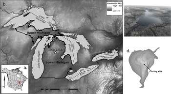
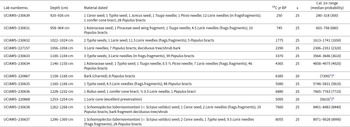
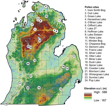
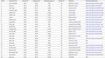
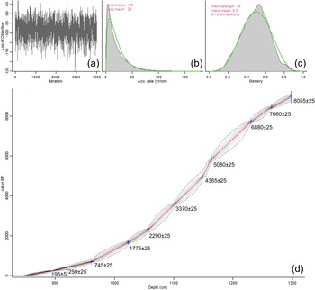
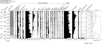

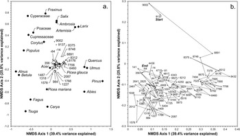


 Open access