


1. Introduction
Frame semantic approaches to semantic and syntactic valency have not only been continuously refined since their inception but also increasingly applied to languages other than English (Boas, Reference Boas, Enghels, Defrancq and Jansegers2020; Boas et al., Reference Boas, Ruppenhofer and Baker2024; Fillmore et al., Reference Fillmore, Lee-Goldman, Rhomieux, Boas and Sag2012). This is also true of the English FrameNet database,Footnote
1 which comprises over 13,000 lexical units in more than 1,000 semantic frames with approximately 200,000 annotated sentences (Ruppenhofer et al., Reference Ruppenhofer, Ellsworth, Petruck, Johnson, Baker and Scheffczyk2016, p. 7). In the broadest sense, the notion of ‘frames’ signifies ‘schematic representations of the conceptual structures and patterns of beliefs, practices, institutions, images, etc. that provide a foundation for meaningful interaction in a given speech community’ (Fillmore et al., Reference Fillmore, Johnson and Petruck2003, p. 235). These frames group lexical units based on the frame elements, that is, the thematic (or $ \theta $
) roles, they evoke (Ruppenhofer et al., Reference Ruppenhofer, Ellsworth, Petruck, Johnson, Baker and Scheffczyk2016, pp. 7–8).
$ \theta $
) roles, they evoke (Ruppenhofer et al., Reference Ruppenhofer, Ellsworth, Petruck, Johnson, Baker and Scheffczyk2016, pp. 7–8).
For instance, verbal lexical units such as boil, brown, or fry are said to evoke the Apply_Heat frame,Footnote 2 in which a COOK applies heat with a certain TEMPERATURE_SETTING to FOOD using a HEATING_INSTRUMENT or a CONTAINER (cf. (1)–(3)).Footnote 3 While these frame element types are mostly specific to the APPLY_HEAT frame, speakers may also choose to supply circumstantial elements, such as MANNER or PLACE, to flexibly modify this or other events. Frame elements are thus assumed to vary with respect to how essential they are to the frame they instantiate: While a cooking event is definitely conceivable without reference to a particular PLACE, this is not possible without a COOK or FOOD.

FrameNet distinguishes between different degrees of ‘coreness’ among the elements evoked as part of a frame. More specifically, there are core and non-core elements, with the core category subsuming core and core-unexpressed elements, and the non-core category peripheral and extra-thematic ones. For example, COOK, FOOD, HEATING_INSTRUMENT and CONTAINER are classified as core to the APPLY_HEAT frame, whereas MEDIUM and PLACE are non-core. The non-core element PLACE is considered to belong to the subset of peripheral elements, which ‘do not introduce additional, independent or distinct events’ (Ruppenhofer et al., Reference Ruppenhofer, Ellsworth, Petruck, Johnson, Baker and Scheffczyk2016, p. 24), while MEDIUM does, thus rendering it extra-thematic. As expected, core-unexpressed elements are rarely attested in FrameNet. The few existing examples list the ACT role, which is said to be evoked as part of the INTENTIONALLY_ACT frame, as a core-unexpressed element (cf. (4)–(5)).

This raises the question of the grounds on which these coreness distinctions are made.
The FrameNet team classifies an element as core if it is (a) realised without exception, (b) assumes a definite reading upon omission, or is (c) formally or semantically idiosyncratic (Ruppenhofer et al., Reference Ruppenhofer, Ellsworth, Petruck, Johnson, Baker and Scheffczyk2016, pp. 23–24). Core-unexpressed elements are claimed to be inherited from more abstract frames, and they are not available for independent realisation, as they are ‘absorbed by the lexical units in the frame’ (Ruppenhofer et al., Reference Ruppenhofer, Ellsworth, Petruck, Johnson, Baker and Scheffczyk2016, p. 25). Of these criteria, only (a) can be directly quantified, suggesting that prototypical core elements occur with a probability equal to 1 or, at the very least, with a probability greater than that of core-unexpressed and non-core elements.Footnote 4 , Footnote 5 However, since FrameNet does not list ‘any statistical information about frequency of occurrence of syntactic patterns or about LUs [lexical units]’ (Fillmore et al., Reference Fillmore, Johnson and Petruck2003, p. 248), this undermines the database’s reliability from a usage-based perspective. Similarly, in light of the quantitative turn of cognitive approaches to language (Janda, Reference Janda2013), the lack of empirical evidence for FrameNet’s coreness labels could potentially undermine theoretical work relying on them.
In particular, research on argument omission would greatly benefit from the empirical validation of FrameNet’s coreness labels. In cognitive linguistics, omission phenomena are subsumed under the notion of Null Instantiation, whose scope only extends to core frame elements (Buskin, Reference Buskin2025, p. 284; Willich, Reference Willich2022, p. 24; Ruppenhofer & Michaelis, Reference Ruppenhofer, Michaelis, Bourns and Lambrecht2014, p. 60; Fillmore, Reference Fillmore1986). For instance, the FrameNet team deems CONTAINER a core element of the APPLY_HEAT frame (cf. (1) earlier); therefore, this thematic role would be considered null-instantiated in (2) and (3), respectively; yet, this would not apply to the putative non-core elements MEDIUM and PLACE. Fundamentally, this issue boils down to what thematic roles can be considered conceptually obligatory for parsing a given event and when this obligatory status is attained.Footnote 6 Arriving at both a usage-based and reproducible method of capturing argument coreness would provide a robust baseline not only for further argument omission research (e.g., Chaves et al., Reference Chaves, Kay and Michaelis2025; Gavruseva, Reference Gavruseva2024) but also for the cross-linguistic study of argument realisation more generally (e.g., Goldberg, Reference Goldberg, Östman and Fried2005).
Previous quantitative research on the core/non-core distinction specifically has been conducted within the context of natural language processing (Matsubayashi et al., Reference Matsubayashi, Okazaki and Tsujii2010; Nikolaev & Padó, Reference Nikolaev, Padó, Amblard and Breitholtz2023). Nikolaev and Padó (Reference Nikolaev, Padó, Amblard and Breitholtz2023) have found that bidirectional encoder representations from transformers (BERT) are capable of distinguishing between core and non-core arguments, displaying substantial frequency effects (Nikolaev & Padó, Reference Nikolaev, Padó, Amblard and Breitholtz2023, p. 235). Yet, the study does not examine the core/non-core contrast itself and does not adduce pertinent accuracy metrics; instead, the emphasis lies on frame identification accuracy. Matsubayashi et al. (Reference Matsubayashi, Okazaki and Tsujii2010) focus on the classification of semantic roles by developing a new softmax classifier that assigns the most plausible frame element label to a constituent, given its frame and formal realisation (Matsubayashi et al., Reference Matsubayashi, Okazaki and Tsujii2010, pp. 850–851). Their data indicate that core and non-core elements can be identified with very high accuracy using frame element descriptors such as SELLER (Matsubayashi et al., Reference Matsubayashi, Okazaki and Tsujii2010, pp. 858–859), which were coined by the FrameNet annotators. Since the objective is to perform accurate semantic role labelling, the plausibility of the coreness labels is inconsequential.
This article addresses two issues: First, it aims to alleviate FrameNet’s empirical opacity by supplementing it with statistical information on the attested combinations of verbs, frames and frame elements. Second, the article examines FrameNet’s empirical plausibility by estimating how well usage data, which is derived from FrameNet’s very own corpus examples, can explain the coreness distinctions made by its annotators. Since ‘usage’ can be conceptualised in different ways, it will be jointly captured in terms of information-theoretic measures and word embeddings, thereby catering to the probabilistic and distributional semantic characteristics of frame elements. Based on this data set, three supervised machine learning models are trained on the usage profiles of all retrieved frame elements to predict the following three coreness distinctions: (i) core versus non-core, (ii) core versus core-unexpressed and (iii) peripheral versus extra-thematic, respectively.
If the usage profiles meaningfully contribute to distinguishing between the different coreness categories, then the models should display high predictive accuracy. I hypothesise that the accuracy will be highest for (expressed) core elements, as this is the only element type for which FrameNet provides an overtly usage-based annotation criterion. Conversely, the remaining coreness types are expected to be less predictable, potentially resulting in poor model performance and hence less grounding in actual language use.
The analysis proceeds as follows: Section 2 formalises frame semantic concepts and their quantification, introduces information-theoretic measures and word embeddings and describes the statistical modelling approach. Section 3 presents results and model evaluation. Section 4 summarises the findings and discusses implications for frame semantics and cognitive linguistics.
2. Methodology
2.1. Formalisation and quantification
The FrameNet database, and hence the derived data set, is characterised by many-to-many relationships between verbs, frames and frame elements. In order to facilitate the statistical analysis, these interrelated sets and relations are formally modelled using set theory. Let $ V $
denote the set of verbs
$ V $
denote the set of verbs $ \left\{{v}_1,{v}_2,\dots, {v}_k\right\} $
, which serve as frame-evoking elements, and
$ \left\{{v}_1,{v}_2,\dots, {v}_k\right\} $
, which serve as frame-evoking elements, and $ F $
the set of all indexed semantic frames
$ F $
the set of all indexed semantic frames $ \left\{{f}_1,{f}_2,\dots, {f}_j\right\} $
. Furthermore, let
$ \left\{{f}_1,{f}_2,\dots, {f}_j\right\} $
. Furthermore, let $ E=\left\{{e}_1,{e}_2,\dots, {e}_t\right\} $
denote the set of all distinct frame elements. These sets are jointly illustrated in Figure 1.Footnote
7 For instance, the lexical unit leave, depending on the context of its occurrence, may evoke the DEPARTING, GIVING, or the ABANDONMENT frame, among others. The participant roles associated with these frames often recur in other frames as well; the THEME argument is common to all three of them, whereas DONOR and AGENT are not. To avoid ambiguity, frame elements should always be characterised with respect to their underlying frame and the evoking verb.
$ E=\left\{{e}_1,{e}_2,\dots, {e}_t\right\} $
denote the set of all distinct frame elements. These sets are jointly illustrated in Figure 1.Footnote
7 For instance, the lexical unit leave, depending on the context of its occurrence, may evoke the DEPARTING, GIVING, or the ABANDONMENT frame, among others. The participant roles associated with these frames often recur in other frames as well; the THEME argument is common to all three of them, whereas DONOR and AGENT are not. To avoid ambiguity, frame elements should always be characterised with respect to their underlying frame and the evoking verb.
Simplified representation of set relations in the FrameNet database.

Consequently, this calls for relations that handle the evocation of frame elements and return the frame structure. To this end, define $ {R}_1\subseteq V\times F $
and
$ {R}_1\subseteq V\times F $
and $ {R}_2\subseteq F\times E $
, so that the set of elements conditioned on a specific verb and a specific frame is given by
$ {R}_2\subseteq F\times E $
, so that the set of elements conditioned on a specific verb and a specific frame is given by
 $$ {E}_v^f=\left\{e\in E:\left(v,f\right)\in {R}_1\wedge \left(f,e\right)\in {R}_2\right\}. $$
Referring to Figure 1, the elements associated with the frame DEPARTING and the verb leave in particular could be represented as follows:
 $$ {E}_{leave}^{\mathrm{DEPARTING}}=\{\mathrm{SOURCE},\mathrm{THEME}\}. $$
To establish the empirical distribution of frame elements in a corpus, all observed elements need to be counted (cf. Definition 2.1.1), giving rise to a discrete probability distribution as in Definition 2.1.2. In order to obtain the observed frequencies and probabilities, an extraction pipeline has been developed using Python’s Natural Language Toolkit (NLTK) FrameNet corpus (version 1.7) (Bird et al., Reference Bird, Loper and Klein2009); the output was subsequently processed in RStudio (RStudio Team, 2020; R version 4.4.2) and Python (Van Rossum & Drake, Reference Van Rossum and Drake2009; Python version 3.13.1). The set of extracted lexical units is limited to verbs, but it could be readily extended to include further parts of speech (see Busse, Reference Busse2012, p. 748). As part of this procedure, data on $ \mid V\mid $
= 2,679 verbs have been obtained, co-occurring with
$ \mid V\mid $
= 2,679 verbs have been obtained, co-occurring with $ \mid E\mid $
= 822 distinct frame elements and representing
$ \mid E\mid $
= 822 distinct frame elements and representing $ \mid F\mid $
= 641 frames in total. For each verbal unit, I processed all attested examples, extracted the annotated frame elements, and aggregated frequency counts for each tuple
$ \mid F\mid $
= 641 frames in total. For each verbal unit, I processed all attested examples, extracted the annotated frame elements, and aggregated frequency counts for each tuple $ \left(v,f,e\right) $
, yielding 21,160 distinct combinations with a total element count of 193,349.
$ \left(v,f,e\right) $
, yielding 21,160 distinct combinations with a total element count of 193,349.
Definition 2.1.1 (Observed frequency). Let $ {N}_v^f $
denote the total number of times verb
$ {N}_v^f $
denote the total number of times verb $ v $
evokes frame
$ v $
evokes frame $ f $
in the corpus. The observed frequency
$ f $
in the corpus. The observed frequency $ {O}_v^f(e) $
of element
$ {O}_v^f(e) $
of element $ e $
given verb
$ e $
given verb $ v $
and frame
$ v $
and frame $ f $
is the count of corpus instances where element
$ f $
is the count of corpus instances where element $ e $
appears when verb
$ e $
appears when verb $ v $
evokes frame
$ v $
evokes frame $ f $
:
$ f $
:
 $$ {O}_v^f(e)=\sum \limits_{i=1}^{N_v^f}\left[\mathrm{element}\hskip0.42em e\hskip0.42em \mathrm{occurs}\ \mathrm{in}\ \mathrm{in}\mathrm{stance}\hskip0.22em i\right] $$
Definition 2.1.2 (Probability mass function). The probability mass function $ {P}_v^f(e) $
returns the probability that element
$ {P}_v^f(e) $
returns the probability that element $ e $
occurs given verb
$ e $
occurs given verb $ v $
and frame
$ v $
and frame $ f $
with
$ f $
with $ {\sum}_{e\in {E}_v^f}{P}_v^f(e)=1 $
. The maximum likelihood estimate is given by
$ {\sum}_{e\in {E}_v^f}{P}_v^f(e)=1 $
. The maximum likelihood estimate is given by
 $$ {P}_v^f(e)=\frac{O_v^f(e)}{\sum_{e\in {E}_v^f}{O}_v^f(e)}. $$
Elements that are theoretically possible but not observed in the corpus (i.e., $ {O}_v^f(e)=0 $
) are excluded from the support of the probability mass function.
$ {O}_v^f(e)=0 $
) are excluded from the support of the probability mass function.
2.2. Frame elements and Zipf’s law
For illustration, the frame element distribution of eat (INGESTION) is presented in Table 1. Note that $ z $
denotes the (Zipfian) frequency rank of an element, which is inversely proportional to its observed frequency. In each case, there are two high-probability elements which contrast with a longer tail of considerably rarer ones.
$ z $
denotes the (Zipfian) frequency rank of an element, which is inversely proportional to its observed frequency. In each case, there are two high-probability elements which contrast with a longer tail of considerably rarer ones.
Frame element distribution of the verb eat in the INGESTION frame with $ N $
= 35
$ N $
= 35

The skewed patterns of these two frame-evoking elements might reflect a more general distributional regularity. In fact, Liu (Reference Liu2011, pp. 211–212) has previously shown that the syntactic complements of English verbs obey a power law. As frame elements can be viewed as semantic complements, it can be hypothesised that frame elements follow a power law as well. By analogy with Baayen (Reference Baayen2001, p. 20), one would need to show that the power model
 $$ {O}_v^f(e)={az}^{-b} $$
reasonably fits the observed data. If the logarithm is taken over both sides, then the respective quantities should be linear in the log–log plane:
 $$ \log {O}_v^f(e)=\log a+b\log z. $$
For instance, regressing $ \log z $
over
$ \log z $
over $ \log {O}_v^f(e) $
returns an
$ \log {O}_v^f(e) $
returns an $ {R}^2 $
of 0.89 for the distribution in Table 1. Repeating this procedure for the 3,875 frame element distributions
$ {R}^2 $
of 0.89 for the distribution in Table 1. Repeating this procedure for the 3,875 frame element distributions $ {E}_v^f $
represented in the FrameNet corpus, least squares solutions could be computed for 3,219. For these cases, it can be confirmed that frame elements follow a Zipfian power law rather well (Mean
$ {E}_v^f $
represented in the FrameNet corpus, least squares solutions could be computed for 3,219. For these cases, it can be confirmed that frame elements follow a Zipfian power law rather well (Mean $ {R}^2 $
= 0.82, SD = 0.11).Footnote
8
$ {R}^2 $
= 0.82, SD = 0.11).Footnote
8
General distributional characteristics of $ {O}_v^f(e) $
and
$ {O}_v^f(e) $
and $ {P}_v^f(e) $
are visualised in Figure 2. Panel A shows the distribution of observed frequencies on a linear scale, exhibiting extreme right-skew, with the vast majority of observations concentrated at very low frequencies. The density curve peaks sharply near zero and decays rapidly, with most frame elements occurring fewer than 50 times. The long tail extends to the most frequent frame element (
$ {P}_v^f(e) $
are visualised in Figure 2. Panel A shows the distribution of observed frequencies on a linear scale, exhibiting extreme right-skew, with the vast majority of observations concentrated at very low frequencies. The density curve peaks sharply near zero and decays rapidly, with most frame elements occurring fewer than 50 times. The long tail extends to the most frequent frame element ( $ {O}_v^f(e)=330 $
), yet only 25% of elements have a frequency greater than 10. Panel B represents the same frequency distribution on a log-scale, revealing some additional structure. The log-frequencies show a more complex distribution with multiple local modes. This pattern suggests distinct ‘tiers’ of element frequencies, approximately binning them into rare, common and highly frequent elements.
$ {O}_v^f(e)=330 $
), yet only 25% of elements have a frequency greater than 10. Panel B represents the same frequency distribution on a log-scale, revealing some additional structure. The log-frequencies show a more complex distribution with multiple local modes. This pattern suggests distinct ‘tiers’ of element frequencies, approximately binning them into rare, common and highly frequent elements.
Density plots of observed (log-)frequencies and sample proportions in the FrameNet data. A: Distribution of observed frequencies. B: Distribution of observed frequencies (log-scale). C: Distribution of element probabilities.

Unsurprisingly, the element probabilities in Panel C similarly demonstrate heavy concentration in the lower value range. The density is highest near zero, with most element having probabilities below 0.10. The distribution continues to show a deep decline followed by several smaller peaks around 0.30–0.50 and approximately 0.60. The long right tail extends to probability values near 1.0, though such cases are very rare.
All of these observations are consistent with pronounced power law behaviour. Regardless, these patterns pose challenges for further statistical inference and, thus, for capturing coreness. Specifically, the extreme sparsity and log-linear structure of frame element distributions call for measures that (a) handle heavily skewed discrete data and (b) respect the logarithmic scaling inherent in power law phenomena. In this regard, information theory provides an apt toolkit for the analysis of argument realisation.
2.3. Information-theoretic framework
Information-theoretic measures are regularly applied in a variety of linguistic subdisciplines, including corpus linguistics (Gries, Reference Gries, Paquot and Gries2020), natural language processing (Manning & Schütze, Reference Manning and Schütze1999), syntactic typology (Levshina, Reference Levshina2019) and psycholinguistics (e.g., Frank et al., Reference Frank, Otten, Galli and Vigliocco2015; Linzen & Jaeger, Reference Linzen and Jaeger2016; Smith & Levy, Reference Smith and Levy2013), among others. Recent advances include information-theoretic studies of valency (Say, Reference Say2025). Since argument realisation is regularly viewed in connection with predictability (e.g., Givón, Reference Givón2017, p. 187 or Goldberg, Reference Goldberg2001, p. 519), and information-theoretic metrics can capture the relative predictability of discrete categories while operating naturally in log-space, they constitute suitable measures for the analysis of frame element distributions. In short, information-theoretic measures represent ‘[d]istributional information for language’ (Slaats & Martin, Reference Slaats and Martin2025, p. 234), which is precisely what is needed for a usage-based characterisation of frame element coreness.
To introduce the basic concepts, recall the set $ {E}_v^f $
, which is a set of discrete categories, and the probability mass function
$ {E}_v^f $
, which is a set of discrete categories, and the probability mass function $ {P}_v^f(e) $
, which returns the probability of observing an element
$ {P}_v^f(e) $
, which returns the probability of observing an element $ e\in {E}_v^f $
. A fundamental measure in information theory is surprisal, which quantifies how unexpected, informative, or surprising a particular outcome is (Cover & Thomas, Reference Cover and Thomas1991, p. 13; Willems et al., Reference Willems, Frank, Nijhof, Hagoort and van den Bosch2016, p. 2507). The surprisal (or information content) of a singular frame element
$ e\in {E}_v^f $
. A fundamental measure in information theory is surprisal, which quantifies how unexpected, informative, or surprising a particular outcome is (Cover & Thomas, Reference Cover and Thomas1991, p. 13; Willems et al., Reference Willems, Frank, Nijhof, Hagoort and van den Bosch2016, p. 2507). The surprisal (or information content) of a singular frame element $ {S}_v^f(e) $
is defined as follows:
$ {S}_v^f(e) $
is defined as follows:
Definition 2.3.1 (Surprisal of frame elements). If $ {P}_v^f(e) $
denotes the probability that a frame element
$ {P}_v^f(e) $
denotes the probability that a frame element $ e $
occurs with verb
$ e $
occurs with verb $ v $
and
$ v $
and $ f $
, then the surprisal of said element is:
$ f $
, then the surprisal of said element is:
 $$ {S}_v^f(e):= -{\log}_2\;{P}_v^f(e)\hskip0.42em \mathrm{with}\hskip0.42em {\log}_2\hskip0.42em 0=0. $$
This value, measured in bits if the logarithmic base is $ 2 $
, increases as the probability
$ 2 $
, increases as the probability $ {P}_v^f(e) $
decreases: Rare (less probable) elements are more informative when they occur and thus have higher surprisal values, as opposed to more common outcomes. As a natural consequence of the log-scaling, small differences in probability are strongly amplified. While the difference between the probabilities 0.03 and 0.01 appears minute (cf. MANNER vs. SOURCE in Table 1), their surprisal equivalents are
$ {P}_v^f(e) $
decreases: Rare (less probable) elements are more informative when they occur and thus have higher surprisal values, as opposed to more common outcomes. As a natural consequence of the log-scaling, small differences in probability are strongly amplified. While the difference between the probabilities 0.03 and 0.01 appears minute (cf. MANNER vs. SOURCE in Table 1), their surprisal equivalents are $ -{\log}_2(0.0345)=3.37 $
and
$ -{\log}_2(0.0345)=3.37 $
and $ -{\log}_2(0.0172)=4.06 $
, respectively. Because frame elements follow a power law and their corresponding probabilities exhibit a strong right-skew, the majority of the probability mass involves low probability elements with small differences in values; surprisal effectively ‘uncompresses’ the probability distribution. This is particularly striking in Figure 3, which exhibits not only more symmetry but also clearer bimodality compared to the untransformed proportions in Figure 2C. Two clusters emerge: uninformative, high probability elements (left peak), and informative, moderate-to-low probability elements (right peak), potentially corresponding to core and non-core elements, respectively.
$ -{\log}_2(0.0172)=4.06 $
, respectively. Because frame elements follow a power law and their corresponding probabilities exhibit a strong right-skew, the majority of the probability mass involves low probability elements with small differences in values; surprisal effectively ‘uncompresses’ the probability distribution. This is particularly striking in Figure 3, which exhibits not only more symmetry but also clearer bimodality compared to the untransformed proportions in Figure 2C. Two clusters emerge: uninformative, high probability elements (left peak), and informative, moderate-to-low probability elements (right peak), potentially corresponding to core and non-core elements, respectively.
Density plot of surprisal in the FrameNet data.

When the weighted sum is taken across all surprisal values in a frame element distribution, we obtain its Shannon entropy $ H\left({E}_v^f\right) $
(cf. Definition 2.3.2), which, in the current application, measures the average information contained in the distribution of frame elements for a given verb
$ H\left({E}_v^f\right) $
(cf. Definition 2.3.2), which, in the current application, measures the average information contained in the distribution of frame elements for a given verb $ v $
and frame
$ v $
and frame $ f $
. This is because Shannon entropy equals the mathematical expectation
$ f $
. This is because Shannon entropy equals the mathematical expectation $ \unicode{x1D53C} $
of
$ \unicode{x1D53C} $
of $ {S}_v^f(e) $
, written
$ {S}_v^f(e) $
, written $ \unicode{x1D53C}\left[{S}_v^f(e)\right] $
.Footnote
9 Since each element’s contribution to the overall entropy is weighted by its occurrence probability, high-probability elements will minimally increase uncertainty, whereas unlikely ones will contribute more substantially. Entropy reaches its maximum value when all outcomes are equally likely (Shannon, Reference Shannon1948), representing the greatest amount of uncertainty in outcomes.Footnote
10 Entropy is low if ‘there are few options, or one of them has a much higher probability than the others’ (Slaats & Martin, Reference Slaats and Martin2025, p. 234). In FrameNet, the entropy of frame element distributions exhibits some bimodality (cf. Figure C1A), indicating that there is a noteworthy set of frames with little uncertainty (
$ \unicode{x1D53C}\left[{S}_v^f(e)\right] $
.Footnote
9 Since each element’s contribution to the overall entropy is weighted by its occurrence probability, high-probability elements will minimally increase uncertainty, whereas unlikely ones will contribute more substantially. Entropy reaches its maximum value when all outcomes are equally likely (Shannon, Reference Shannon1948), representing the greatest amount of uncertainty in outcomes.Footnote
10 Entropy is low if ‘there are few options, or one of them has a much higher probability than the others’ (Slaats & Martin, Reference Slaats and Martin2025, p. 234). In FrameNet, the entropy of frame element distributions exhibits some bimodality (cf. Figure C1A), indicating that there is a noteworthy set of frames with little uncertainty ( $ {H}_v^f\approx 1 $
).Footnote
11 As a distribution-level feature, entropy characterises semantic valency patterns as a whole, revealing the degree of asymmetry in argument realisation preference.
$ {H}_v^f\approx 1 $
).Footnote
11 As a distribution-level feature, entropy characterises semantic valency patterns as a whole, revealing the degree of asymmetry in argument realisation preference.
Definition 2.3.2 (Entropy of a frame element distribution). Suppose every element $ e\in {E}_v^f $
has probability
$ e\in {E}_v^f $
has probability $ {P}_v^f(e) $
and surprisal
$ {P}_v^f(e) $
and surprisal $ {S}_v^f(e) $
. The entropy of the corresponding frame element distribution, written
$ {S}_v^f(e) $
. The entropy of the corresponding frame element distribution, written $ H\left({E}_v^f\right) $
, is:
$ H\left({E}_v^f\right) $
, is:
 $$ H\left({E}_v^f\right)=-\sum \limits_{e\in {E}_v^f}{P}_v^f(e)\;{\log}_2\;{P}_v^f(e). $$
A useful consequence of Definitions 2.3.1 and 2.3.2 is that the surprisal of each individual outcome $ e\in {E}_v^f $
can be compared to the average surprisal of the whole distribution. That is, one can calculate a deviation score that captures whether a frame element is more or less informative than expected in its distribution. This can be achieved in a way that respects the sign of the difference (cf. Definition 2.3.3) or instead emphasises the absolute difference by analogy with squared errors (cf. Definition 2.3.4). Some general statistical properties of (squared) entropy deviation are given in Appendix A. By analogy with the other measures, entropy deviation exhibits a bimodal distribution in the FrameNet data (Figure C1B), with a substantial portion of elements clustering slightly below 0.
$ e\in {E}_v^f $
can be compared to the average surprisal of the whole distribution. That is, one can calculate a deviation score that captures whether a frame element is more or less informative than expected in its distribution. This can be achieved in a way that respects the sign of the difference (cf. Definition 2.3.3) or instead emphasises the absolute difference by analogy with squared errors (cf. Definition 2.3.4). Some general statistical properties of (squared) entropy deviation are given in Appendix A. By analogy with the other measures, entropy deviation exhibits a bimodal distribution in the FrameNet data (Figure C1B), with a substantial portion of elements clustering slightly below 0.
Definition 2.3.3 (Entropy deviation). Let $ {S}_v^f(e) $
denote the surprisal of a frame element and
$ {S}_v^f(e) $
denote the surprisal of a frame element and $ H\left({E}_v^f\right) $
the entropy of its frame element distribution. Then, entropy deviation expresses how much more (or less) surprising a specific outcome
$ H\left({E}_v^f\right) $
the entropy of its frame element distribution. Then, entropy deviation expresses how much more (or less) surprising a specific outcome $ e $
is upon occurrence compared to the expected level of surprise in the distribution:
$ e $
is upon occurrence compared to the expected level of surprise in the distribution:
 $$ {\Delta}_v^f(e):= {S}_v^f(e)-H\left({E}_v^f\right). $$
Definition 2.3.4 (Squared entropy deviation). Suppose $ {\Delta}_v^f(e) $
captures the entropy deviation of an element
$ {\Delta}_v^f(e) $
captures the entropy deviation of an element $ e $
. The squared entropy deviation captures how strongly this element deviates from
$ e $
. The squared entropy deviation captures how strongly this element deviates from $ H\left({E}_v^f\right) $
:
$ H\left({E}_v^f\right) $
:
 $$ {\left[{\Delta}_v^f(e)\right]}^2:= {\left[{S}_v^f(e)-H\left({E}_v^f\right)\right]}^2. $$
The total spread of surprisal values around their expected value is their variance and is known as varentropy; in other words, it ‘measures the variability in the information content’ (Di Crescenzo & Paolillo, Reference Di Crescenzo and Paolillo2021, p. 682) of a random variable:
Definition 2.3.5 (Varentropy). The total variance of surprisal values in a frame element distribution is the varentropy $ \unicode{x1D54D}\left[{S}_v^f(e)\right] $
.
$ \unicode{x1D54D}\left[{S}_v^f(e)\right] $
.
It can be easily shown that varentropy is the expected (i.e., average) squared deviation of surprisal values from the distributional average (cf. Proposition A.2). When comparing their corresponding histograms (cf. Figure C1C and C1D), frame elements typically cluster quite closely around the expected surprisal (entropy), suggesting little deviation overall.
2.4. Word vectors
Distributional semantic models represent word meaning on the basis of usage patterns in large corpora and have proven highly informative in the synchronic and diachronic study of English lexis, morphology and syntax (e.g., Hamilton et al., Reference Hamilton, Leskovec, Jurafsky, Erk and Smith2016; Marelli & Baroni, Reference Marelli and Baroni2015; Perek, Reference Perek2016; Shafaei-Bajestan et al., Reference Shafaei-Bajestan, Uhrig and Baayen2022). These approaches are fundamentally usage-based in that semantic content is approximated via statistical word co-occurrence patterns in representative collections of authentic linguistic data (Boleda, Reference Boleda2020, pp. 214–215; Günther et al., Reference Günther, Rinaldi and Marelli2019).Footnote 12
In the present study, distributional semantic representations are used to characterise the semantic profiles of FrameNet frame elements. While information-theoretic measures capture how frequently elements occur in particular frames, word embeddings may capture what semantic content typically fills a given frame element. Rather than modelling concrete phrasal or clausal realisations directly, the analysis abstracts away from surface structure and focuses on the aggregate semantic properties of frame element fillers. To this end, pre-trained word embeddings from the fastText library (Bojanowski et al., Reference Bojanowski, Grave, Joulin and Mikolov2017; Mikolov et al., Reference Mikolov, Grave, Bojanowski, Puhrsch, Joulin, Calzolari, Choukri, Cieri, Declerck, Goggi, Hasida, Isahara, Maegaard, Mariani, Mazo, Moreno, Odijk, Piperidis and Tokunaga2018; Mouselimis, Reference Mouselimis2024) were extracted for all attested frame element fillers in the FrameNet database. These embeddings incorporate subword information and are therefore well suited to modelling morphologically complex and low-frequency items.
At the level of individual corpus instances, frame elements realised by a single word are represented by that word’s embedding, while multi-word realisations are represented by the unweighted average of the embeddings of their constituent words. This procedure reflects the assumption that words jointly realising a frame element contribute equally to its semantic interpretation, and it avoids introducing additional parameters for which no independent weighting criteria are available. To obtain distributional representations at the level required for the present analysis, these token-level representations are further aggregated across all attestations of a given verb–frame–element combination. The resulting frame element embeddings thus capture the typical distributional semantic profile of a frame element as it is realised with a particular verb and frame. A fully formal specification of the embedding construction and aggregation procedure is provided in Appendix B.
2.5. Machine learning methods
The statistical analysis in this study uses ensembles of boosted decision trees with random effects, implemented via the Gaussian Process Boosting (GPBoost) framework (Sigrist, Reference Sigrist2022). This approach combines the strengths of tree-based machine learning (such as decision trees and random forests, which are already familiar in corpus linguistics; e.g., Tagliamonte & Baayen, Reference Tagliamonte and Baayen2012) with mixed-effects modelling. In essence, GPBoost enables the modelling of complex, non-linear relationships between predictors and outcomes while also accounting for hierarchical structure in the data (Sigrist, Reference Sigrist2022, p. 1).
For each coreness distinction, I fit a mixed-effects model with both fixed and random effects and compare it to a null model with random effects only. Information-theoretic measures and word vectors constitute the fixed effects, and ‘verb’ as well as ‘frame’ the grouping factors. Formally, the model predicts the response vector $ \mathbf{y} $
(e.g., whether an element is core or non-core) following Equation (11).
$ \mathbf{y} $
(e.g., whether an element is core or non-core) following Equation (11).
 $$ \mathbf{y}=F(\mathbf{X})+\mathbf{Z}\mathbf{b}+\boldsymbol{\epsilon} \hskip1em \mathrm{w}\mathrm{i}\mathrm{t}\mathrm{h}\hskip0.4em \mathbf{b}\sim \mathcal{N}(\mathbf{0},\boldsymbol{\Sigma} ),\boldsymbol{\epsilon} \sim \mathcal{N}(\mathbf{0},{\sigma}^2{\mathbf{I}}_n) $$ $ F\left(\mathbf{X}\right) $
is the set of boosted trees used to approximate the relationship between the independent variables
$ F\left(\mathbf{X}\right) $
is the set of boosted trees used to approximate the relationship between the independent variables $ \mathbf{X} $
and the target variable,
$ \mathbf{X} $
and the target variable, $ \mathbf{Zb} $
represents random effects, and
$ \mathbf{Zb} $
represents random effects, and $ \boldsymbol{\epsilon} $
is the model error. The grouping factor is assumed to follow a multivariate normal distribution with mean vector
$ \boldsymbol{\epsilon} $
is the model error. The grouping factor is assumed to follow a multivariate normal distribution with mean vector $ \boldsymbol{\mu} =\mathbf{0} $
and covariance matrix
$ \boldsymbol{\mu} =\mathbf{0} $
and covariance matrix $ \boldsymbol{\Sigma} $
, and the residuals should be independent and identically distributed normal variables.
$ \boldsymbol{\Sigma} $
, and the residuals should be independent and identically distributed normal variables.
Model fitting in GPBoost proceeds via gradient boosting, where each decision tree is sequentially added to minimise prediction error by following the direction of steepest descent in the loss function (gradient descent; see Hastie et al., Reference Hastie, Tibshirani and Friedman2017, pp. 358–360, for details). To ensure robust predictive performance, hyperparameters (such as tree depth and learning rate) are optimised using randomised grid search with binary log-loss (cross-entropy) as the minimisation criterion. All models are trained and validated in Python’s scikit-learn environment (Pedregosa et al., Reference Pedregosa, Varoquaux, Gramfort, Michel, Thirion, Grisel, Blondel, Prettenhofer, Weiss, Dubourg, Vanderplas, Passos, Cournapeau, Brucher, Perrot and Duchesnay2011), with the data split into 75% training and 25% test sets to assess overfitting.
Predictive performance is evaluated using standard classification metrics, namely, accuracy, AUC, precision, recall and the F1-score; their calculation is summarised in Table 2. In addition, the Matthews Correlation Coefficient (MCC, see Equation 12) will be reported by analogy with Yoffe et al. (Reference Yoffe, Dershowitz, Vishne and Sober2025, p. 10). The MCC is the confusion matrix analogue of Pearson’s $ r $
, ranging from −1 (all labels misclassified) to +1 (all labels correctly classified), with 0 representing the random baseline (Chicco & Jurman, Reference Chicco and Jurman2020, p. 5). It can only be high if both positive cases are consistently identified correctly (i.e., high precision and recall) and negative ones are as well. As such, for each of the three coreness contrasts, it will provide a joint metric of how well both outcomes can be predicted.
$ r $
, ranging from −1 (all labels misclassified) to +1 (all labels correctly classified), with 0 representing the random baseline (Chicco & Jurman, Reference Chicco and Jurman2020, p. 5). It can only be high if both positive cases are consistently identified correctly (i.e., high precision and recall) and negative ones are as well. As such, for each of the three coreness contrasts, it will provide a joint metric of how well both outcomes can be predicted.
 $$ \mathrm{MCC}=\frac{TP\cdot TN- FP\cdot FN}{\sqrt{\left( TP+ FP\right)\cdot \left( TP+ FN\right)\cdot \left( TN+ FP\right)\cdot \left( TN+ FN\right)}} $$
Summary of common classification metrics (TP = true positive, TN = true negative, FP = false positive, FN = false negative) based on Chicco and Jurman (Reference Chicco and Jurman2023, pp. 2–3), Alpaydın (Reference Alpaydın2022, pp. 632–636) and James et al. (Reference James, Witten, Hastie and Tibshirani2021, pp. 148–152)

3. Results
The information-theoretic measures introduced in Section 2.3 can be harnessed to capture fine-grained quantitative characteristics of the right-skewed frame element distributions. Table 3 revisits the INGESTION frame and provides information-theoretic metrics for each element. It is worth noting that some elements appear to be less surprising than expected upon occurrence ( $ {\Delta}_v^f<0 $
), while some are more surprising (
$ {\Delta}_v^f<0 $
), while some are more surprising ( $ {\Delta}_v^f>0 $
). At the same time, two elements, which are in fact core elements of this frame, are very close to the expected surprisal of elements in this frame (
$ {\Delta}_v^f>0 $
). At the same time, two elements, which are in fact core elements of this frame, are very close to the expected surprisal of elements in this frame ( $ {[{\Delta}_v^f]}^2\approx 0 $
), while the non-core elements are substantially further away (
$ {[{\Delta}_v^f]}^2\approx 0 $
), while the non-core elements are substantially further away ( $ {\left[{\Delta}_v^f\right]}^2\gg 0 $
). This pattern is remarkably consistent across a variety of verb-frame combination (cf. Figure 4), albeit not categorical; some putative core elements (e.g., DELIVERY_DEVICE in Panel E) pattern more closely to non-core elements.
$ {\left[{\Delta}_v^f\right]}^2\gg 0 $
). This pattern is remarkably consistent across a variety of verb-frame combination (cf. Figure 4), albeit not categorical; some putative core elements (e.g., DELIVERY_DEVICE in Panel E) pattern more closely to non-core elements.
Probability distribution of frame elements conditioned on the verb eat and the frame INGESTION with a Shannon entropy $ H({E}_{eat}^{\mathrm{INGESTION}}) $
of 1.85 bits and a varentropy of 1.38
$ H({E}_{eat}^{\mathrm{INGESTION}}) $
of 1.85 bits and a varentropy of 1.38

Surprisal $ {S}_v^f(e) $
, Shannon entropy (dashed line) and entropy deviation (solid horizontal lines) of frame element types conditioned on verbs in different frames.
$ {S}_v^f(e) $
, Shannon entropy (dashed line) and entropy deviation (solid horizontal lines) of frame element types conditioned on verbs in different frames.

3.1. Descriptive overview
The frame element types are distributed unevenly (see Table 4), with core elements constituting half of all realised elements, peripheral ones a third and extra-thematic ones approximately one-sixth. Core-unexpressed elements are rare at less than 1% of occurrences. Table 5 presents descriptive statistics on the observed usage data. Particularly striking is the asymmetry and extreme tailedness in the observed counts: Typically, the element distributions derived from the FrameNet data involve low-frequency and low-probability elements while still allowing for substantial outliers. This pattern aptly reflects the data reported in Table 3 earlier. It also applies to the squared entropy deviation, albeit in a strongly attenuated form, as the bulk of elements tend to be rather close to the expected surprisal of their distribution.
Distribution of element types for all verbs in the FrameNet database

Summary statistics on the predictor variables ( $ n $
= 21,160)
$ n $
= 21,160)

Figure 5 illustrates the conditional distributions of element probabilities and information-theoretic measures by element coreness. Given that counts are sample-dependent, the estimated proportions are provided in Figure 5A. These data show that the vast majority of non-core elements show low probabilities of occurrence, with only one out 10,278 exceeding the 0.5 probability mark. By contrast, core elements are considerably more spread out, taking on values across the entire [0, 1] interval, with 75% lying below 0.42. Accordingly, core and core-unexpressed elements concentrate around lower surprisal values (Panel 5B), which correspond to probabilities of occurrence close to 1, but display negative skew with long tails. Non-core elements show more symmetric distributions with notably higher surprisal values; for reference, a surprisal of 5 corresponds to a probability of $ {2}^{-5}=0.03 $
and a value of 7.5 to
$ {2}^{-5}=0.03 $
and a value of 7.5 to $ {2}^{-7.5}=0.006 $
.
$ {2}^{-7.5}=0.006 $
.
Distribution of information-theoretic measures across frame element types (density plots). A: Distribution of $ {P}_v^f(e) $
by coreness. B: Distribution of
$ {P}_v^f(e) $
by coreness. B: Distribution of $ {S}_v^f(e) $
by coreness. C: Distribution of
$ {S}_v^f(e) $
by coreness. C: Distribution of $ {\Delta}_v^f(e) $
by coreness. D: Distribution of
$ {\Delta}_v^f(e) $
by coreness. D: Distribution of $ [{\Delta}_v^f(e){]}^2 $
by coreness.
$ [{\Delta}_v^f(e){]}^2 $
by coreness.

When examining the entropy deviations (Panel C), core elements cluster closely around the average surprisal of their distributions, with the majority having deviation scores less than 0, reflecting the intuition that core elements are less surprising than expected upon occurrence. Extra-thematic and peripheral elements consistently show positive entropy deviations, carrying more information than average. The squared deviation (Panel D) highlights the magnitude of these deviations regardless of direction. On the whole, the squared deviation scores are right-skewed, with a small subset of frame elements exhibiting exceptionally large departures from expected surprisal values. Non-parametric Dunn tests reveal no significant differences between core and core-unexpressed elements across any information-theoretic measure, while all other pairwise comparisons between coreness types are statistically significant (cf. Table 6).
Dunn test results with Bonferroni-adjusted $ p $
-values (
$ p $
-values ( $ {p}_{\mathrm{adjusted}} $
) for pairwise comparisons between frame element types based on three entropy-derived metrics
$ {p}_{\mathrm{adjusted}} $
) for pairwise comparisons between frame element types based on three entropy-derived metrics

Prior to model fitting, it is worth inspecting the pairwise feature correlations in Table 7 to rule out mutual redundancies. In fact, the determinant of the matrix is 0, rendering it singular and non-invertible. Due to perfect collinearity between probability and surprisal, and given the information-theoretic approach pursued here, surprisal is retained as the more theoretically motivated measure of element predictability. Moreover, raw observed counts were excluded due to their sample dependence, as absolute frequencies may reflect corpus composition rather than inherent usage patterns. The analysis instead focuses on distributional properties that capture relative predictability across different verb-frame combinations.
Feature correlation matrix based on Spearman’s $ \rho $

3.2. Model evaluation
Tables 8 and 9 compare the overall predictive performance of the mixed-effects gradient boosting models with and without usage data. The corresponding metrics are visualised in Figure 6.Footnote
13 Usage data provide substantial improvements for the core versus non-core distinction, with MCC increasing from 0.542 to 0.817 and accuracy from 0.527 to 0.907. As for the peripheral versus extra-thematic contrast, the MCC only improves marginally (MCC: 0.533 $ \to $
0.556). The core versus core-unexpressed distinction shows high accuracy in both models (
$ \to $
0.556). The core versus core-unexpressed distinction shows high accuracy in both models ( $ > $
0.98), though this largely reflects class imbalance given the extreme rarity of core-unexpressed elements (0.89% of cases). Quite strikingly, the MCC for this contrast decreases from 0.813 to 0.538 with the addition of usage data, indicating that the null model’s apparent success was driven by predicting the majority class rather than genuine discriminative power.
$ > $
0.98), though this largely reflects class imbalance given the extreme rarity of core-unexpressed elements (0.89% of cases). Quite strikingly, the MCC for this contrast decreases from 0.813 to 0.538 with the addition of usage data, indicating that the null model’s apparent success was driven by predicting the majority class rather than genuine discriminative power.
General performance metrics for the full model with fixed and random effects (95% confidence intervals); MCC normalised to [0,1] scale

General performance metrics for the random-effects-only model (95% confidence intervals); MCC normalised to [0,1] scale

Summary of general performance metrics (dashed line represents expected values if the model was guessing randomly).

Class-specific metrics (Tables 10 and 11, Figure 7) reveal distinct patterns across contrasts. For core versus non-core, the full model achieves balanced performance (F1 $ \approx $
0.919 for both classes), while the null model defaults to predicting ‘core’ for nearly all instances (non-core recall = 0.040). This demonstrates that distributional information is essential for this distinction.
$ \approx $
0.919 for both classes), while the null model defaults to predicting ‘core’ for nearly all instances (non-core recall = 0.040). This demonstrates that distributional information is essential for this distinction.
Class-specific performance metrics for the Full Model (95% confidence intervals)

Class-specific performance metrics for the random-effects-only model (95% confidence intervals)

Summary of class-specific test performance with 95% CIs.

The core versus core-unexpressed contrast presents a different challenge. While core elements are predicted near-perfectly (F1 = 0.994), core-unexpressed elements exhibit extreme variance with confidence intervals spanning [0.000, 1.000] for both precision and recall. This instability persists even with usage data, suggesting insufficient training instances for stable pattern learning.Footnote 14 Counterintuitively, the full model’s MCC (0.538) is substantially lower than the null model’s (0.813), though both exhibit wide confidence intervals. This pattern suggests that while the null model achieves moderate balanced performance by relying on structural patterns alone, the addition of usage features destabilises predictions for the rare core-unexpressed class without providing sufficient discriminative information.
For peripheral versus extra-thematic, the full model shows asymmetric performance: Peripheral elements are identified accurately (F1 = 0.884, recall = 0.980), while extra-thematic elements show high precision (0.910) but poor recall (0.453). The model correctly identifies extra-thematic elements when it predicts this label but misclassifies over half as peripheral. The null model defaults to predicting ‘extra-thematic’ for most instances (recall = 0.997), failing to identify peripheral elements (recall = 0.025). Despite similar MCC values between models (0.533 vs. 0.556), the full model achieves substantially higher accuracy (0.821 vs. 0.319), indicating that usage data enable meaningful classification where the null model cannot distinguish the categories.
Finally, the covariance parameters for the three models differ only in terms of frames, as they were consistently zero for the verbs. The core/non-core model showed the smallest contribution of frames as a random effect (0.13), closely followed by the peripheral/extra-thematic one (0.17). The outcomes of the core/core-unexpressed distinction, by contrast, were heavily affected by the frame under consideration (2.42), indicating that frame identity explains substantial between-frame variation in core-unexpressed classification.
3.3. Feature importance and partial dependence
The relative contributions of individual predictors are visualised in Figures 8 and 9. These plots include only predictors whose bootstrapped 95% confidence intervals exclude zero after 250 resampling iterations, indicating reliable non-zero contributions to model performance. While considerable overlap exists between confidence intervals across features, several patterns emerge. For the core versus non-core distinction (Figure 8), entropy deviation $ {\Delta}_v^f(e) $
and word vector dimension V163 emerge as the strongest predictors. Intermediate contributors include surprisal
$ {\Delta}_v^f(e) $
and word vector dimension V163 emerge as the strongest predictors. Intermediate contributors include surprisal $ {S}_v^f(e) $
, V80 and V95. The peripheral versus extra-thematic distinction (Figure 9) is dominated by word vector dimensions V163, surprisal, and V134. No feature importance plot is presented for the core versus core-unexpressed contrast, as all predictors displayed confidence intervals spanning zero or including negative values, reflecting the instability discussed above.
$ {S}_v^f(e) $
, V80 and V95. The peripheral versus extra-thematic distinction (Figure 9) is dominated by word vector dimensions V163, surprisal, and V134. No feature importance plot is presented for the core versus core-unexpressed contrast, as all predictors displayed confidence intervals spanning zero or including negative values, reflecting the instability discussed above.
Feature importance scores for the core versus non-core distinction with bootstrapped 95% CIs (‘H_vf’ = $ H\left({E}_v^f\right) $
, ‘Se_vf’ =
$ H\left({E}_v^f\right) $
, ‘Se_vf’ = $ {S}_v^f(e) $
, ‘Dev_S_H’ =
$ {S}_v^f(e) $
, ‘Dev_S_H’ = $ {\Delta}_v^f(e) $
, ‘Dev_sq_S_H’ =
$ {\Delta}_v^f(e) $
, ‘Dev_sq_S_H’ = $ {\left[{\Delta}_v^f(e)\right]}^2 $
).
$ {\left[{\Delta}_v^f(e)\right]}^2 $
).

Feature importance scores for the extra-thematic versus peripheral distinction with bootstrapped 95% CIs.

Partial dependence plots (Figures 10–12) reveal the functional form of these relationships. For core versus non-core, $ {\Delta}_v^f(e) $
shows a robust positive effect: Non-core status becomes increasingly likely as an element’s surprisal exceeds the distribution’s entropy (i.e.,
$ {\Delta}_v^f(e) $
shows a robust positive effect: Non-core status becomes increasingly likely as an element’s surprisal exceeds the distribution’s entropy (i.e., $ {\Delta}_v^f(e)>0 $
). At
$ {\Delta}_v^f(e)>0 $
). At $ {\Delta}_v^f(e)=2 $
, the predicted probability of ‘non-core’ is approximately 0.25 times higher than the model’s average prediction. Surprisal
$ {\Delta}_v^f(e)=2 $
, the predicted probability of ‘non-core’ is approximately 0.25 times higher than the model’s average prediction. Surprisal $ {S}_v^f(e) $
shows a weaker effect, with probability increases becoming relevant only for values
$ {S}_v^f(e) $
shows a weaker effect, with probability increases becoming relevant only for values $ \ge 3 $
; the effect of varentropy is markedly non-linear. Positive loadings of the word vector dimensions in Figure 11 appear to be associated with core status. Remarkably, higher V163 scores increase the probability that a frame element is a core element, and lower scores are linked to peripheral non-core elements. Surprisal appears to be marginally lower for peripheral elements compared to extra-thematic ones.
$ \ge 3 $
; the effect of varentropy is markedly non-linear. Positive loadings of the word vector dimensions in Figure 11 appear to be associated with core status. Remarkably, higher V163 scores increase the probability that a frame element is a core element, and lower scores are linked to peripheral non-core elements. Surprisal appears to be marginally lower for peripheral elements compared to extra-thematic ones.
Partial dependence of the core versus non-core model (information-theoretic measures).

Partial dependence of the core versus non-core model (word vectors).

Partial dependence of the extra-thematic versus peripheral model.

4. Discussion
4.1. Summary and limitations
The present study examined whether FrameNet’s coreness distinctions are grounded in actual language use by training machine learning models on information-theoretic measures and word embeddings to predict three coreness contrasts: (i) core versus non-core, (ii) core versus core-unexpressed and (iii) peripheral versus extra-thematic. The choice of information-theoretic predictors was motivated by the finding that frame elements follow Zipf’s law, making entropy-based measures particularly well-suited to capturing their predictability patterns. Word embeddings complement this approach by capturing the semantic profiles of frame element fillers grounded in authentic language use. The results provide clear but differentiated support for these distinctions:
-
1) The core versus non-core contrast showed strong usage-based grounding. The full model achieved near-perfect classification, with entropy deviation $ {\Delta}_v^f(e) $
emerging as the strongest predictor. Crucially, the null model containing only lexical and frame information failed catastrophically, demonstrating the importance of usage data. Partial dependence analysis additionally reveals important quantitative characteristics of core elements:
$ {\Delta}_v^f(e) $
emerging as the strongest predictor. Crucially, the null model containing only lexical and frame information failed catastrophically, demonstrating the importance of usage data. Partial dependence analysis additionally reveals important quantitative characteristics of core elements:-
– Core elements display
$ {\Delta}_v^f(e)\le 0 $
. Their information content is systematically below the average (entropy) of the frame element distribution. -
– Core elements minimise
$ {S}_v^f(e) $
. They are highly likely to occur and thus do not convey much new information upon occurrence. -
– Core elements minimise
$ {\left[{\Delta}_v^f(e)\right]}^2 $
. They cluster relatively closely around the entropy of the frame element distribution. -
– Core elements maximise word vectors V163, V80, V95 and V169. Thus, they exhibit characteristic distributional semantic profiles.
-
-
2) The peripheral versus extra-thematic distinction showed moderate usage-based support. The classifier relied on semantic features (word vectors V163 and V134) as well as on surprisal, which did not raise the general performance metrics above the random baseline. They did, however, improve the class-specific performance, especially the identification of peripheral elements. In particular, these display the following features:
-
– Peripheral elements minimise
$ {S}_v^f(e) $
. Their information content is on the lower end, yet it is higher than that of core elements. -
– Peripheral elements minimise V163, and they display a non-linear association with V134.
-
-
3) The core versus core-unexpressed contrast proved empirically problematic. Despite high overall accuracy, this reflected class imbalance rather than genuine discriminative success. Confidence intervals for core-unexpressed precision and recall spanned [0.000, 1.000], indicating extreme instability across bootstrap samples. It is, therefore, not surprising that no relevant predictors could be identified. It is likely that the rarity of core-unexpressed elements (0.89% of cases) prevented stable pattern learning, raising questions about whether this constitutes a coherent coreness category.


Overall, the results indicate that FrameNet’s core-non-core distinction is robustly usage-based, while finer-grained coreness subtypes lack consistent distributional grounding, highlighting both the empirical strengths and theoretical limits of FrameNet’s current annotation system.
Several limitations suggest directions for future research. The analysis is restricted to verbal lexical units in English; extension to other parts of speech and languages would test cross-linguistic validity. The extreme rarity of core-unexpressed elements warrants targeted investigation with expanded data collection or clearer annotation guidelines. The semantic content of influential word vector dimensions (particularly V163) remains unexplored and could reveal deeper connections between distributional semantics and argument structure. Finally, pursuing an unsupervised rather than supervised machine learning approach could reveal whether coreness distinctions naturally emerge from the feature space.Footnote 15
4.2. Implications
4.2.1. For frame semantics and FrameNet
The present findings have non-negligible implications for frame semantics and the architecture of FrameNet. First, the strong performance of information-theoretic measures in distinguishing core from non-core elements validates the intuition in the literature that coreness fundamentally reflects argument predictability. This interpretation aligns with FrameNet’s criterion that a core element ‘always has to be overtly specified’ (Ruppenhofer et al., Reference Ruppenhofer, Ellsworth, Petruck, Johnson, Baker and Scheffczyk2016, p. 23), which translates empirically to high probability and low surprisal. However, the current analysis reveals that this probability-based criterion is less diagnostic than entropy deviation, that is, the predictability of an element relative to the frame’s average. More broadly, these findings provide strong empirical support for the traditional argument/adjunct dichotomy, suggesting that while individual borderline cases exist, the core/non-core boundary reflects genuine distributional patterns.
The failure of the core versus core-unexpressed distinction raises more fundamental questions about FrameNet. Core-unexpressed elements, by definition, lack surface realisation and should not occur to begin with. The extreme instability in classification performance suggests that this category may not constitute a coherent distributional class but rather an idiosyncratic collection of annotations that are strongly frame-dependent, as was suggested by the elevated frame covariance parameter. The category’s theoretical basis (elements ‘absorbed by the lexical units in the frame’; Ruppenhofer et al., Reference Ruppenhofer, Ellsworth, Petruck, Johnson, Baker and Scheffczyk2016, p. 25) may describe a semantic or lexical phenomenon that does not manifest in usage patterns. From a usage-based perspective, this disconnect between theoretical motivation and empirical realisation warrants reconsideration of whether core-unexpressed should be treated as a coreness category at all, potentially justifying their removal from FrameNet.
The peripheral versus extra-thematic distinction presents a different challenge. Usage data primarily improve the identification of peripheral elements, which exhibit distinct surprisal and word vector patterns. Entropy deviation is probably no longer helpful because non-core elements predominantly concentrate in the high deviation region, with peripheral ones being slightly less surprising than extra-thematic ones. What is striking is the importance of word vector dimension V163 across both core/non-core and peripheral/extra-thematic tasks, suggesting it may encode a general semantic property of participant roles or coreness, though further investigation of its content is needed, as word vectors are notoriously challenging to interpret (see Günther et al., Reference Günther, Rinaldi and Marelli2019, for an in-depth discussion). In short, it appears likely that there are at least two subpopulations among the non-core elements, yet they are more difficult to delimit than in the core/non-core case.
4.2.2. For cognitive research in argument realisation
The empirical validation of the core versus non-core distinction has direct consequences for research on argument null instantiation and for argument realisation more generally. Since null instantiation is conventionally restricted to core frame elements, establishing which elements qualify as core is foundational to defining the phenomenon’s scope. Previous work has lacked an empirical basis for this determination, potentially including non-core elements in null instantiation analyses or excluding legitimate core elements. The information-theoretic and distributional semantic criteria examined in this study provide a principled and reproducible method for the identification of conceptually essential arguments across languages.
Given the features summarised in Section 4.1, it is possible to develop a coreness annotation pipeline without the need for computationally expensive classifiers. If, at the very least, frequency counts are available, an entropy-based decision rule could be used: An element $ e\in {E}_v^f $
belongs to the set of core elements
$ e\in {E}_v^f $
belongs to the set of core elements $ {C}_v^f\subseteq {E}_v^f $
if and only if entropy deviation is less than or equal to zero (cf. Equation 13), that is,
$ {C}_v^f\subseteq {E}_v^f $
if and only if entropy deviation is less than or equal to zero (cf. Equation 13), that is,
 $$ {C}_v^f=\left\{e\in {E}_v^f:{\Delta}_v^f(e)\le 0\right\}. $$
To validate this measure, the mixed-effects gradient boosting model was refitted with entropy deviation as a single predictor, yielding very good performance for both core (Precision = 0.89, Recall = 0.81, F1 = 0.85) and non-core outcomes (Precision = 0.82, Recall = 0.89, F1 = 0.85) with a normalised MCC of 0.85. As such, this very simple model is basically equivalent to the full, complex model reported in Table 8 earlier. Although this criterion may perform well as a practical decision rule, assuming a sharp boundary necessarily involves loss in nuance and further disregards the subtle influence of other distributional factors.
Data availability statement
The data that support the findings of this study are openly available in this OSF repository: https://osf.io/n74e9.
Competing interests
The author reports that there are no competing interests to declare.
Appendix A Information theory
Proposition A.1 (Property of entropy deviation). Let $ {S}_v^f(e) $
denote the surprisal of element
$ {S}_v^f(e) $
denote the surprisal of element $ e $
and
$ e $
and $ H\left({E}_v^f\right)=\unicode{x1D53C}\left[{S}_v^f(e)\right] $
the entropy of its corresponding frame element distribution. Then, the entropy deviation
$ H\left({E}_v^f\right)=\unicode{x1D53C}\left[{S}_v^f(e)\right] $
the entropy of its corresponding frame element distribution. Then, the entropy deviation $ {\Delta}_v^f(e) $
satisfies:
$ {\Delta}_v^f(e) $
satisfies:
 $$ \unicode{x1D53C}\left[{\Delta}_v^f(e)\right]=0. $$
Proof.
 $$ \unicode{x1D53C}\left[{\Delta}_v^f(e)\right]=\sum \limits_e\;{P}_v^f(e)\hskip0.1em \left({S}_v^f(e)-H\left({E}_v^f\right)\right) $$
 $$ =\sum \limits_e\;{P}_v^f(e){S}_v^f(e)-H\left({E}_v^f\right)\sum \limits_e\;{P}_v^f(e) $$
 $$ =H\left({E}_v^f\right)-H\left({E}_v^f\right) $$
 $$ =0. $$
Proposition A.2 (Entropy variance). The expectation of the squared entropy deviation corresponds to the varentropy of the frame element distribution:
 $$ \unicode{x1D53C}\left[{\left[{\Delta}_v^f(e)\right]}^2\right]=\unicode{x1D54D}\left[{S}_v^f(e)\right]. $$
Proof. The variance of a random variable $ X $
is defined as follows:
$ X $
is defined as follows:
 $$ \unicode{x1D54D}\left[X\right]:= \unicode{x1D53C}\left[{X}^2\right]-{\left(\unicode{x1D53C}\left[X\right]\right)}^2. $$
Therefore, the goal is to show that:
 $$ \unicode{x1D53C}\left[{\left[{\Delta}_v^f(e)\right]}^2\right]=\unicode{x1D53C}\left[{S}_v^f(e)\right]-{\left(\unicode{x1D53C}\left[{S}_v^f(e)\right]\right)}^2. $$
After applying the definition of expectation (cf. Equation 7) to $ {[{\Delta}_v^f(e)]}^2 $
, expanding the square and summarising the remaining terms, the identity in Equation 21 follows naturally.
$ {[{\Delta}_v^f(e)]}^2 $
, expanding the square and summarising the remaining terms, the identity in Equation 21 follows naturally.
 $$ \unicode{x1D53C}\left[{\left[{\Delta}_v^f(e)\right]}^2\right]=\sum \limits_e\;{P}_v^f(e){\left[{S}_v^f(e)-H\left({E}_v^f\right)\right]}^2 $$
 $$ =\sum \limits_e\;{P}_v^f(e)\left[{S}_v^f{(e)}^2-2{S}_v^f(e)H\left({E}_v^f\right)+H{\left({E}_v^f\right)}^2\right] $$
 $$ =\sum \limits_e\;{P}_v^f(e){S}_v^f{(e)}^2-\sum \limits_e\;{P}_v^f(e)2{S}_v^fH\left({E}_v^f\right)+\sum \limits_e\;{P}_v^f(e)H{\left({E}_v^f\right)}^2 $$
 $$ =\sum \limits_e\;{P}_v^f(e){S}_v^f{(e)}^2-2H\left({E}_v^f\right)H\left({E}_v^f\right)+H{\left({E}_v^f\right)}^2 $$
 $$ =\sum \limits_e\;{P}_v^f(e){S}_v^f{(e)}^2-H{\left({E}_v^f\right)}^2 $$
 $$ =\unicode{x1D53C}\left[{S}_v^f{(e)}^2\right]-{\left(\unicode{x1D53C}\left[{S}_v^f(e)\right]\right)}^2\hskip1em \left(\mathrm{definition}\ \mathrm{of}\ \mathrm{variance}\right) $$
 $$ =\unicode{x1D54D}\left[{S}_v^f(e)\right] $$
Appendix B Formal specification of word vector construction
This appendix provides a formal specification of the procedures used to construct distributional semantic representations of FrameNet frame elements.
B.1. Frame element realisation
For each occurrence $ i $
in which verb
$ i $
in which verb $ v $
evokes frame
$ v $
evokes frame $ f $
(where
$ f $
(where $ i=1,2,\dots, {N}_v^f $
), let
$ i=1,2,\dots, {N}_v^f $
), let $ {\mathcal{W}}_i^{(v,f)}(e) $
denote the ordered sequence of words that realise frame element
$ {\mathcal{W}}_i^{(v,f)}(e) $
denote the ordered sequence of words that realise frame element $ e $
in that occurrence:
$ e $
in that occurrence:
 $$ {\mathcal{W}}_i^{(v,f)}(e)=({w}_1,{w}_2,\dots, {w}_{n_i}), $$
where
![]() is the number of words in the realisation of element
is the number of words in the realisation of element $ e $
in occurrence
$ e $
in occurrence $ i $
. If element
$ i $
. If element $ e $
is not present in occurrence
$ e $
is not present in occurrence $ i $
, then
$ i $
, then
![]() .
.
B.2 Word embeddings
Let $ \varphi :W\to {\mathrm{\mathbb{R}}}^d $
denote the word embedding function that maps each word
$ \varphi :W\to {\mathrm{\mathbb{R}}}^d $
denote the word embedding function that maps each word $ w\in W $
(the vocabulary) to a
$ w\in W $
(the vocabulary) to a $ d $
-dimensional vector representation, where
$ d $
-dimensional vector representation, where $ d $
is the embedding dimensionality.
$ d $
is the embedding dimensionality.
For each occurrence $ i $
of verb
$ i $
of verb $ v $
evoking frame
$ v $
evoking frame $ f $
, the sequence of word vectors corresponding to the realisation of frame element
$ f $
, the sequence of word vectors corresponding to the realisation of frame element $ e $
is defined as follows:
$ e $
is defined as follows:
 $$ {\Phi}_i^{\left(v,f\right)}(e)=\left(\varphi \left({w}_1\right),\varphi \left({w}_2\right),\dots, \varphi \left({w}_{n_i}\right)\right), $$
where $ {w}_j\in {\mathcal{W}}_i^{(v,f)}(e) $
for
$ {w}_j\in {\mathcal{W}}_i^{(v,f)}(e) $
for $ j\in \left\{1,2,\dots, {n}_i\right\} $
. If
$ j\in \left\{1,2,\dots, {n}_i\right\} $
. If
![]() , then
, then
![]() .
.
B.3 Frame element vector representations
To obtain a single vector representation for each realised frame element, three cases are distinguished. If a frame element is not realised in a given occurrence, no vector representation is defined. If it is realised by a single word, the corresponding word embedding is used. If it is realised by multiple words, the unweighted arithmetic mean of their embeddings is computed.
Formally, the vector representation $ {\mathbf{v}}_i^{\left(v,f\right)}(e) $
of frame element
$ {\mathbf{v}}_i^{\left(v,f\right)}(e) $
of frame element $ e $
in occurrence
$ e $
in occurrence $ i $
is defined as follows:
$ i $
is defined as follows:

Instances for which
![]() are excluded from subsequent aggregation.
are excluded from subsequent aggregation.
Since the analysis operates at the level of verb–frame–element combinations, token-level frame element vectors are further aggregated across all attestations. Let $ {O}_v^f(e) $
denote the observed frequency of element
$ {O}_v^f(e) $
denote the observed frequency of element $ e $
with verb
$ e $
with verb $ v $
in frame
$ v $
in frame $ f $
. The aggregated vector representation of frame element
$ f $
. The aggregated vector representation of frame element $ e $
is then given by the following:
$ e $
is then given by the following:
 $$ {\mathbf{v}}_v^f(e)=\frac{1}{O_v^f(e)}\sum \limits_{i:e\;\mathrm{attested}\ \mathrm{in}\;i}{\mathbf{v}}_i^{\left(v,f\right)}(e). $$
These aggregated vectors, which represent centroids of all token-level vectors in embedding space, constitute the distributional semantic representations used in the main analysis.
Appendix C Supplementary Figures
Unconditional distributions of information-theoretic measures (density plots). A: Distribution of entropy. B: Distribution of entropy deviation. C: Distribution of squared entropy deviation. D: Distribution of varentropy.


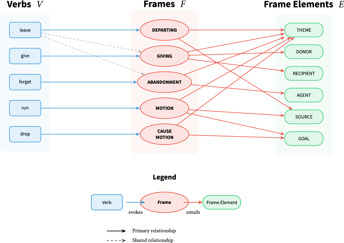
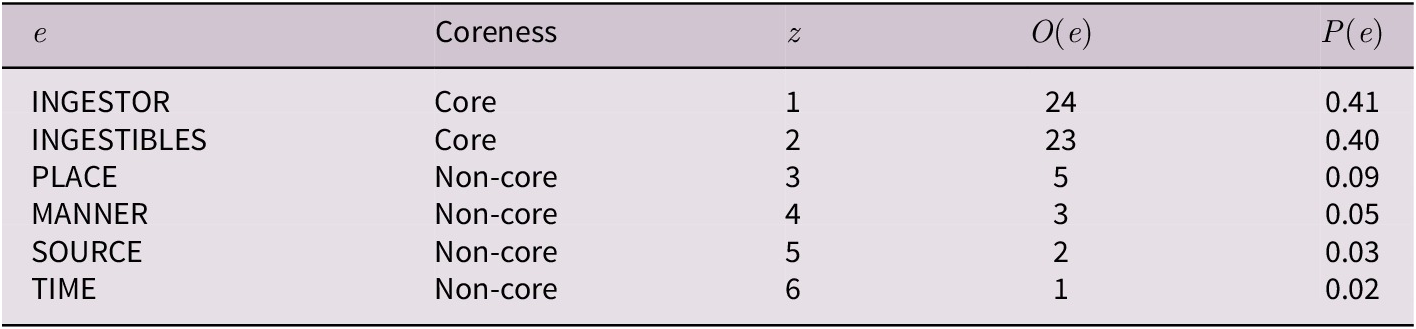

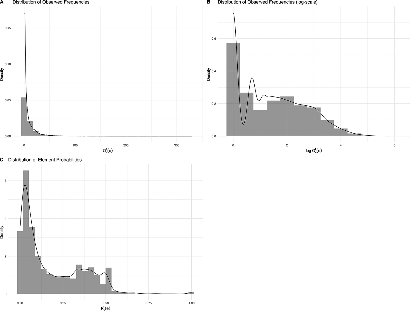
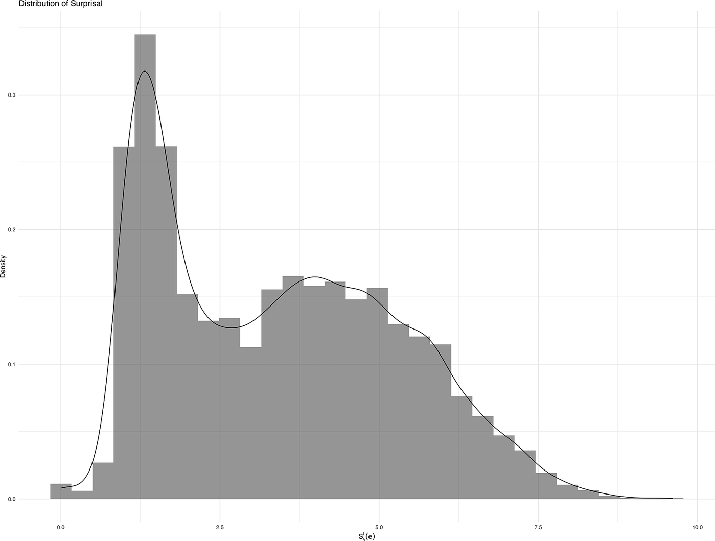

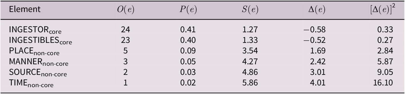

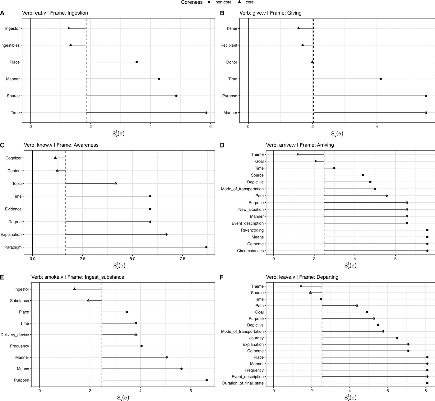

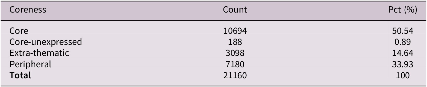


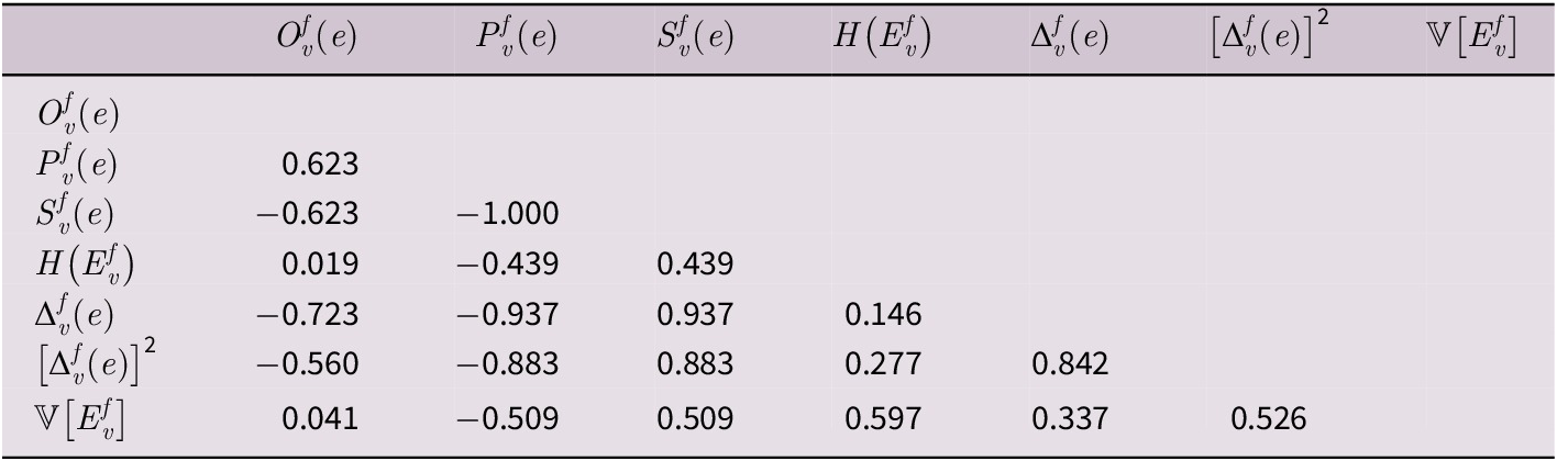


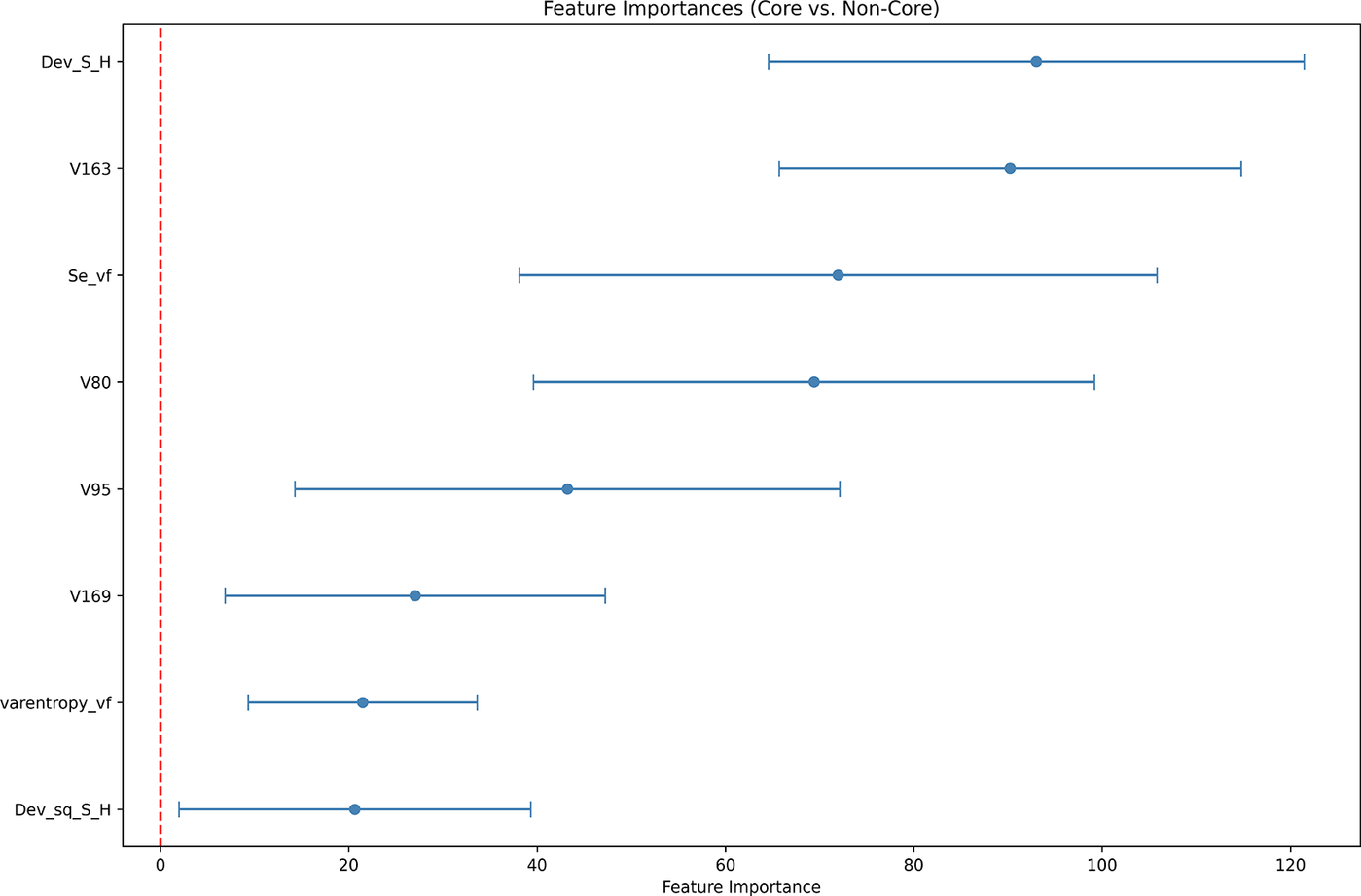


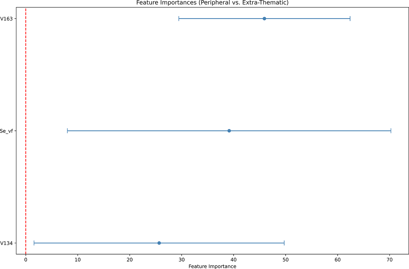


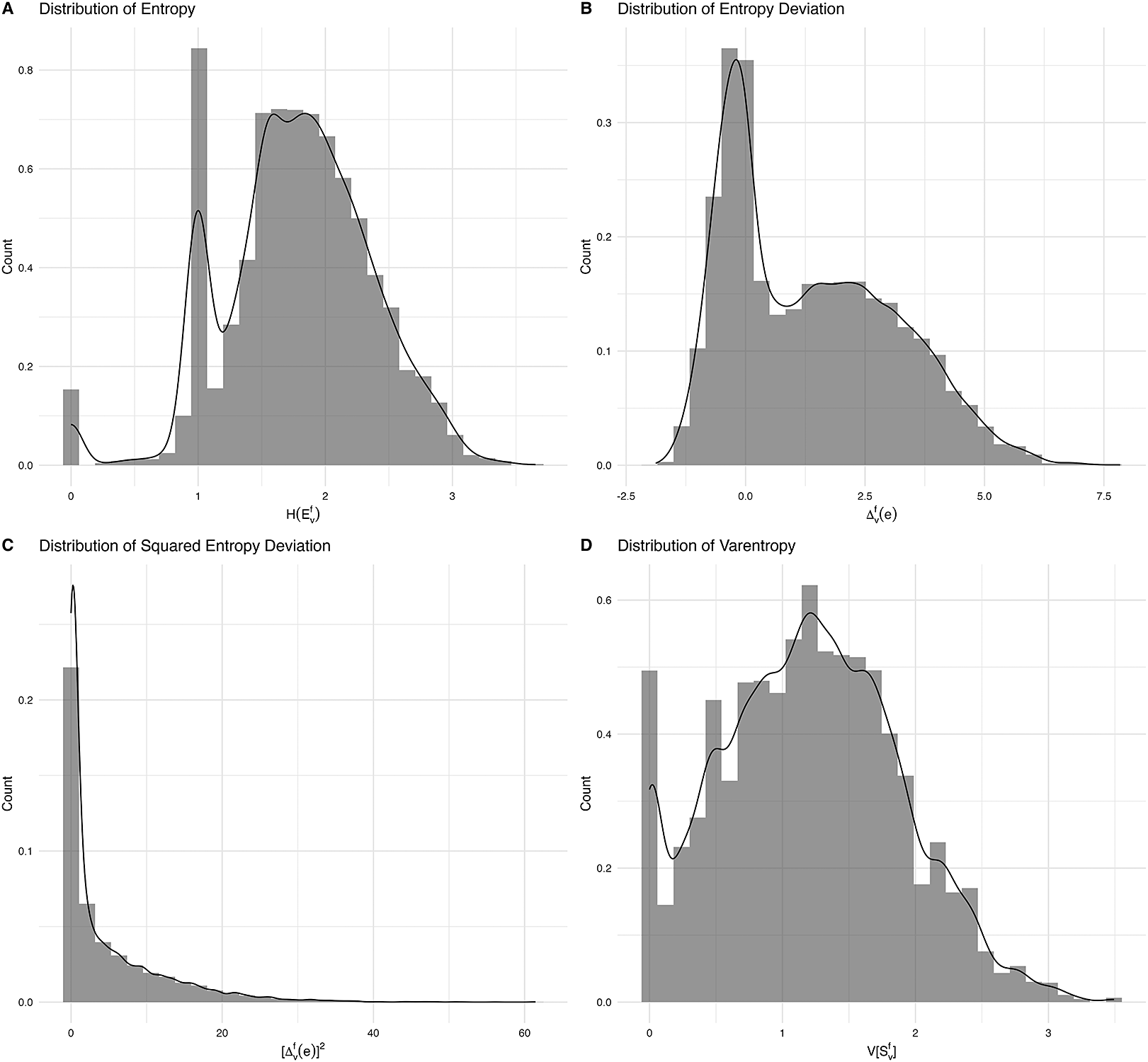

 Open access