


Introduction and study area
Canada contains about  $185,000\,\mathrm{km}^{2}$ of glacierised terrain, about one quarter of the global total area outside of the ice sheets (RGI 7.0 Consortium, 2023), and most of these glaciers are rapidly retreating. Glaciers in Western Canada experienced an acceleration in the rate of area loss by a factor of $\sim$7 between 1984–2010 and 2011–20 (Bevington and Menounos, Reference Bevington and Menounos2022). Acceleration continued over the past four years as mass loss nearly doubled from 2010–19 to 2020–24 (Menounos and others, Reference Menounos, Huss, Marshall, Ednie, Florentine and Hartl2025). This mass loss occurred primarily through widespread surface thinning driven by warm, dry conditions and general darkening of glacier surfaces.
Given the importance of glacier runoff to Canada’s economy, the federal government established a network of glacier monitoring sites during the International Hydrological Decade (Ommanney, Reference Ommanney1986). These sites became operational in 1965 and, ten years later, the Government of Canada added Helm Glacier to the inventory (Ommanney and others, Reference Ommanney, Demuth and Meier2002). Helm Glacier is a World Glacier Monitoring Service (WGMS) reference glacier and only one of seven glaciers in Canada where mass balance observations exceed 40 years. Helm Glacier ( $49^{\circ}57'29''\,\mathrm{N}$, $122^{\circ}59'13''\,\mathrm{W}$, RGI60-02.00377) lies on the western edge of Garibaldi Provincial Park, British Columbia, Canada, in the Pacific Ranges of the southern Coast Mountains and in the traditional territory of the Squamish Nation (Fig. 1). As of April 2025, the small ( $0.35\,\mathrm{km}^{2}$) glacier spanned an elevation range from $1780\,\mathrm{m}$ a.s.l. to $2150\,\mathrm{m}$ a.s.l. Helm Glacier reached its maximum Holocene extent ( $4.5\,\mathrm{km}^{2}$) at about 1690-1710 CE (Koch and others, Reference Koch, Menounos and Clague2009). Except for a period of slowed recession with a minor advance between the late 1960s and 1970s, Helm Glacier experienced widespread thinning with attendant shrinkage throughout the Twentieth Century. In 1928, Helm Glacier had an area of approximately
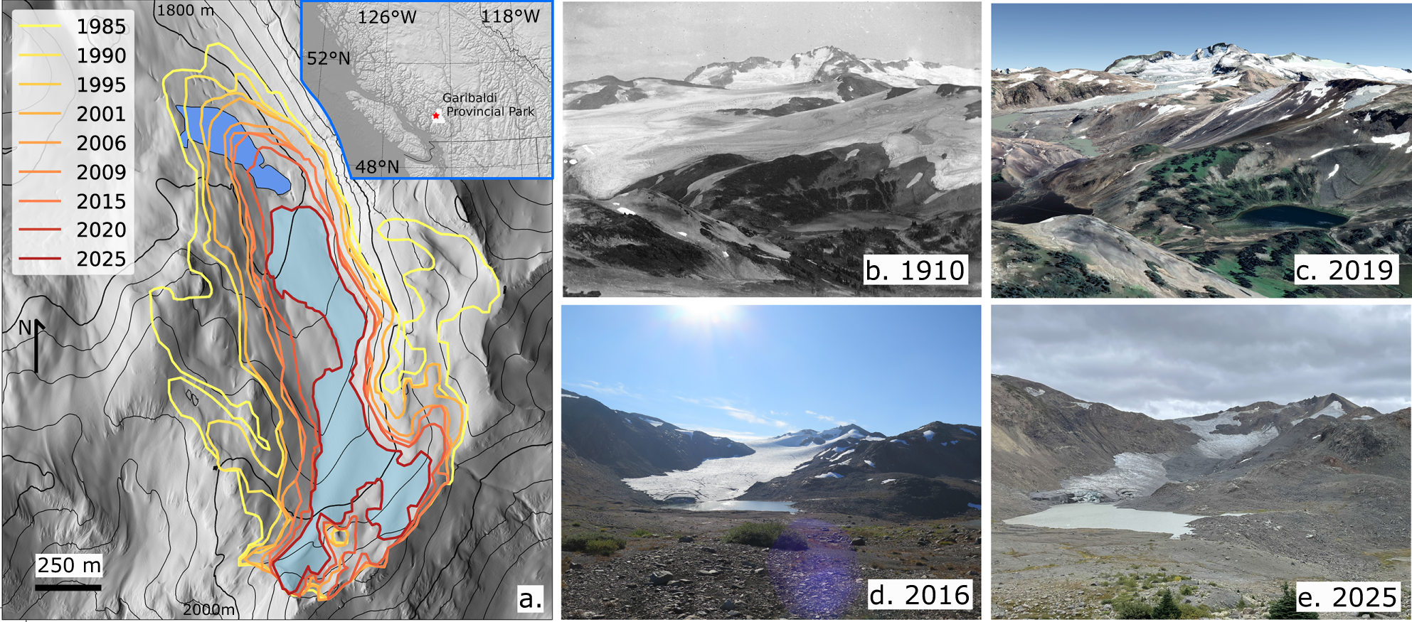
  $4.28\,\mathrm{km}^2$, losing over 80% of its area by 2005 (Koch and others, Reference Koch, Menounos and Clague2009) with an average area loss rate of roughly 3.5% per year from 1985 to 2025 (Fig. 2, see Supplementary Material for details of historic area change). Pronounced retreat of Helm Glacier led to the formation of a proglacial lake around 1990. Thinning over the last eight years led to fragmentation of the glacier in its uppermost elevations, eventually fragmenting the upper and lower glaciers in the fall of 2025.
(a) 2025 glacier extent (red outline with blue fill) with historic glacier outlines traced from end-of-summer spaceborne Landsat imagery and airborne ortho-imagery. Topography is shown using a 2025 LiDAR hillshade with 50 m contour intervals (see Supplementary Material for methods and acquisition dates). Inset showing Helm Glacier (red star) within Garibaldi Provincial Park and in the traditional territory of the Squamish Nation. Proglacial lake shown in dark blue. (b) Oblique image of Helm Glacier in 1910s (unknown photographer, courtesy of City of Vancouver Archives). (c) Google Earth Engine image (6 Aug, 2019 imagery) shown from approximately the same location as (b). (d) Helm Glacier in 2016 (M. Ednie) and (e) from approximately the same location in 2025 (M. Ednie).

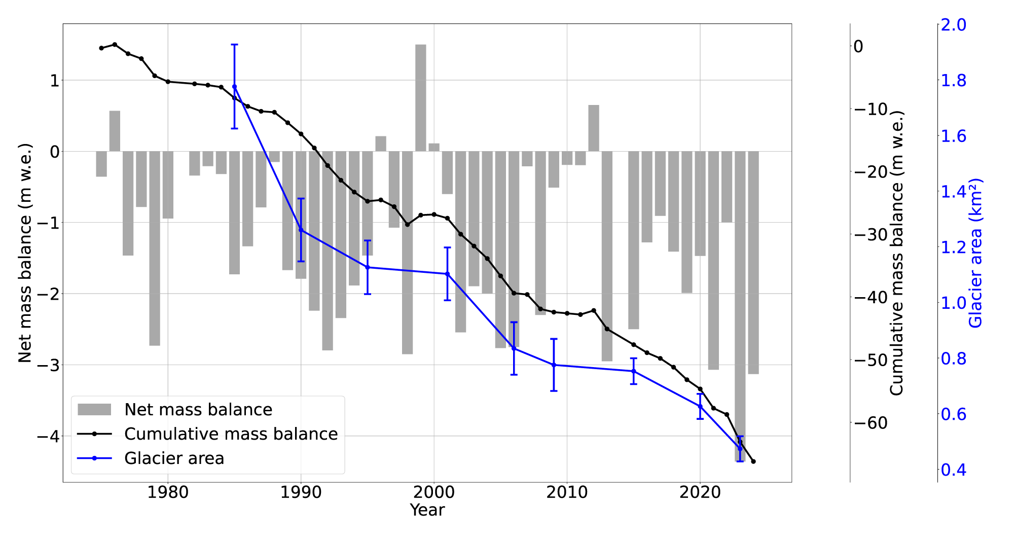
Annual mass balance (grey bars) and cumulative mass balance (dotted black line) at Helm Glacier from WGMS (2024) plotted with the glacier area (blue line, contours shown in Figure 1). The error in glacier area is computed from the product of the perimeter and the image resolution (see Table S1).

In situ observations at Helm Glacier have been collected since 1975 and use the stratigraphic method (e.g. Kaser and others, Reference Kaser, Fountain and Jansson2003). Along a series of centreline stakes, ablation is measured in late September, while snow thickness and snow density (measured in snow pits at two of the stakes) are measured in late April. Balance measurements are binned into elevation bands that are summed to yield a glacier-wide net mass balance. Based on the mass balance record (WGMS, 2024), Helm Glacier experienced only five years of positive mass balance since 1975 (Fig. 2). Recent imagery and mass balance surveys of the glacier reveal widespread loss of firn with negligible accumulation area, especially from 2021 to 2025. In situ data averaged over the last seven years show an annual balance at the terminus of  $-3.6\,\mathrm{m\,w.e}.$, $-1.6\,\mathrm{m}$ w.e. at the summit and a glacier-wide net mass balance of $-2.3\,\mathrm{m}$ w.e. During that time period, the winter balance averaged over the entire glacier was $1.85\,\mathrm{m}$ w.e. Helm Glacier experienced its most extreme year of mass loss in 2023 ( $-4.34\,\mathrm{m w.e}$.), roughly 2.5 times greater than the average of the previous six years (Menounos and others, Reference Menounos, Huss, Marshall, Ednie, Florentine and Hartl2025).
From 1984 to 2025, Helm Glacier experienced the most negative climatic mass balance of all 16 WGMS monitored glaciers in North America (WGMS, 2024), implying high sensitivity to temperature changes or enhanced local warming. A rapid decrease in area, fragmentation and a strongly negative mass balance all point towards glacier extinction in the near future, indicating that an important WGMS long-term monitoring site will be lost. In this work, our primary objectives are to: (1) project the timing of extinction for Helm Glacier; and (2) investigate the drivers of mass balance and mass balance sensitivity.
Methods
In situ observations at Helm Glacier provide invaluable validation data and long-term mass balance records (e.g. Zemp and others, Reference Zemp2019), but for small alpine glaciers these point measurements cannot capture the complex spatial variability in mass balance arising from snow redistribution (McGrath and others, Reference McGrath2015; Pulwicki and others, Reference Pulwicki, Flowers, Radić and Bingham2018; Kneib and others, Reference Kneib2024) or topographic shading (Olson and Rupper, Reference Olson and Rupper2019). Automatic weather station (AWS) data can help validate energy balance and accumulation models, but AWS datasets similarly lack spatial coverage and are not available at Helm Glacier. To overcome these limitations, we use repeat laser altimetry to quantify the spatial distribution of surface elevation change that cannot be resolved with lower-resolution satellite products or in situ measurements (Beedle and others, Reference Beedle, Menounos and Wheate2014; Pelto and others, Reference Pelto, Menounos and Marshall2019). Accurate knowledge of ice thickness is also essential for predicting the timing of disappearance of small alpine glaciers (Langhammer and others, Reference Langhammer, Grab, Bauder and Maurer2019; Millan and others, Reference Millan, Mouginot, Rabatel and Morlighem2022), so we conduct an ice-penetrating radar survey to constrain the bed topography. These datasets allow us to develop a multivariate statistical regression essential for modelling area change and mass balance sensitivity of Helm Glacier.
Ice thickness and surface topography
On 21 May, 2025, we completed an ice-penetrating radar survey of Helm Glacier on skis. The Blue Systems Integration Ltd. radar system uses resistively-loaded dipole antennas with a centre frequency of 10 MHz, has 12-bit resolution and yields a sampling rate of up to 250 Megasamples per second (Mingo and Flowers, Reference Mingo and Flowers2010). The radar system contains a single frequency global navigation satellite system (GNSS) with an accuracy of  $\pm5\,\mathrm{m}$. The antenna spacing was $15\,\mathrm{m}$ and we assume a velocity through ice at $1.68 \times 10^{8}\,\mathrm{m\,s}^{-1}$ (Reynolds, Reference Reynolds2011). We processed the radar data with IceRadarAnalyzer processing software (Blue System Integration Ltd, version 6.3.1 beta). To increase the signal-to-noise ratio of the data, we averaged 128 stacks for each trace in the radargram and then applied gain and filtering for the identification of bed reflectors. Using a $10 \times 10\,\mathrm{m}$ grid, we compute a map of the ice thickness from a 2D linear interpolation of the radar data with the boundary of the glacier set to zero thickness. Taking i) the uncertainty as the mean of the ice thickness at intersecting transects, ii) the uncertainty of one-quarter of the radar wavelength (Reynolds, Reference Reynolds2011) and iii) the uncertainty that arises from surface slope within a $10 \times 10\,\mathrm{m}$ grid cell, we estimate the total error in ice thickness by propagating the error in quadrature.
To measure the glacier surface elevation, we carry out end-of-ablation season repeat LiDAR surveys from 2020 to 2024, carried out by the Hakai-UNBC Airborne Coastal Observatory (acquisition dates given in Table S1). LiDAR was acquired by a 1064-nm laser equipped with an inertial measurement unit and GNSS, yielding a vertical accuracy of  $\pm 0.5\,\mathrm{m}$ (Donahue and others, Reference Donahue2023; Menounos and others, Reference Menounos, Huss, Marshall, Ednie, Florentine and Hartl2025). We derive four yearly surface elevation change maps that are co-registered using the XDEM package (https://pypi.org/project/xdem/) following methods described in Nuth and Kääb (Reference Nuth and Kääb2011) and Hugonnet and others (Reference Hugonnet2022). Elevation change maps are downsampled to $10\,\mathrm{m}$ ground spacing distance to match the ice thickness grid.
To increase the vertical accuracy of the ice-penetrating radar survey, we carried out additional LiDAR survey on 24 April, 2025. Observations of surface elevation change from a sonic depth ranger equipped with satellite telemetry (Bevington and others, Reference Bevington, Menounos and Ednie2025) reveals about  $1\,\mathrm{m}$ of thinning between our LiDAR and radar surveys.
Projection of glacier disappearance
We use an area of  $0.01\,\mathrm{km}^{2}$ to define the threshold at which point Helm Glacier would cease to exist (RGI 7.0 Consortium, 2023). To estimate the year when this will occur, we forward model the yearly surface elevation change of Helm Glacier using two approaches. In our first simple approach, we extrapolate the four year average surface elevation change at each grid cell forward in time by subtracting this average change from the ice thickness grid each year. Ice vanishes from a grid cell when the cumulative elevation change exceeds the grid cell ice thickness, and the area is recomputed at each time step.
For the second approach, we use multivariate regression to model elevation change. Regression models of surface mass balance of individual glaciers or collections of glaciers are commonly carried out on direct explanatory variables such as temperature and precipitation (Lliboutry, Reference Lliboutry1974; Letréguilly, Reference Letréguilly1988), or indirect synoptic-scale climate indices (Moore and Demuth, Reference Moore and Demuth2001; Shea and Marshall, Reference Shea and Marshall2007). Here we use four years of data to fit a distributed model over the glacier surface, though a minimum of ten years of data would be ideal (Letréguilly, Reference Letréguilly1988; Vincent and Vallon, Reference Vincent and Vallon1997; Zekollari and Huybrechts, Reference Zekollari and Huybrechts2018). We model surface elevation change  $\mathbf{dh}$ based on the design matrix $\mathbf{X}$. The regression $\mathbf{dh} = \mathbf{X} \boldsymbol{\beta} + \boldsymbol{\varepsilon}$ is computed from the $n=3540$, $10 \times 10\,\mathrm{m}$ grid cells from data concatenated across four glaciological years from 2021 to 2024. The matrix $\mathbf{X}$ is composed of slope ( $\boldsymbol{\theta}$), orientation ( $\boldsymbol{\alpha}$), positive-degree days ( $\mathbf{PDD}$), masked shortwave radiation at the surface ( $\mathbf{SW_{\downarrow}}$) and snow depth ( $\mathbf{s}$). The optimal coefficients are estimated through least-squares regression as, $\hat{\boldsymbol{\beta}} = (\mathbf{X}^\top \mathbf{X})^{-1} \mathbf{X}^\top \mathbf{dh}$. These bulk $\hat{\boldsymbol{\beta}}$-values are tested on each of the $j^{th}$ years individually as $\hat{\mathbf{dh}}^{j} = \mathbf{X}^{j} \hat{\boldsymbol{\beta}}$, with the $R^2$ computed between the yearly difference in observed and modelled elevation change at each grid cell.
Computed PDDs are summed in the time intervals given by the LiDAR acquisition dates (Table S1) as  $\mathbf{PDD}_j = \sum T(z)$ for $T \gt 0^{\circ}$C. The temperature ( $T$) is taken from dynamically downscaled hourly ERA-5 land temperatures (Hersbach and others, Reference Hersbach2020) given at the nearest grid point $4.5\,\mathrm{km}$ from the centre of the glacier ( $50^{\circ}$N, $123^{\circ}$W) and lapsed up from $1550\,\mathrm{m}$ to the elevation of each grid cell. Similar to the melt-season lapse rate computed by Shea and others (Reference Shea, Moore and Stahl2009) of $-6.0^{\circ}\mathrm{C\,km}^{-1}$, we calculate an April-to-October average lapse rate of $-5.8^{\circ}\mathrm{C\,km}^{-1}$ from 2021 to 2025 based on three BC Hydro weather stations within $20\,\mathrm{km}$ of Helm Glacier. We compute annual snow depth for the glacier using snow depth collected each April at six locations along the glacier centreline. We derive a polynomial fit between snow depth and elevation to compute an elevation-dependent snow-depth field. Summer (May-Sept) incoming shortwave radiation is computed by multiplying a shading factor matrix computed in the HORAYZON v1.2 model (Steger and others, Reference Steger, Steger and Schär2022) with the mean of the daily averaged downwelling shortwave radiation obtained from the nearest gridpoint of ERA5-Land reanalysis. Although the shading model and surface normal shortwave radiation both depend on surface slope and aspect, we include slope and aspect as independent variables to capture other mass balance processes that may affect snow depth (Fig. S1).
To forward model elevation change and area, we start with the 2024 DEM and force the model with the average of the yearly PDD fields from 2014 to 2024, all computed at the 2024 grid cell elevations with a start date of October 31. The forcing for  $\mathbf{SW}_{\downarrow}$ and the snow depth field ( $\mathbf{s}$) are generated from averaging the 2020–24 fields used in the regression model. At each yearly time step, we recompute the surface elevation, slope, aspect, PDDs and snow-depth fields, but keep $\mathbf{SW}_{\downarrow}$ fixed in time. We estimate uncertainty in elevation change by initialising the ice thickness with the error bounds derived from the radar survey. Given the widespread loss of firn, the modelled elevation change does not depend on firn densification.
Mass balance sensitivity
We test the net mass balance ( $B_n$) sensitivity of our model to changes in temperature as $\mathrm{C_T} = \partial B_n/ \partial T$ and precipitation as $\mathrm{C_P} = \partial B_n/ \partial P$. Sensitivities are computed using the $\hat{\boldsymbol{\beta}}$-values obtained in the regression model, but we vary the mean summer temperature and the mean winter balance (e.g. Cuffey and Paterson, Reference Cuffey and Paterson2010), then model the change in mass balance one year into the future, neglecting firn densification and ice dynamics. We test the sensitivity of i) yearly specific mass balance using the 2024 reference surface (e.g. Elsberg and others, Reference Elsberg, Harrison, Echelmeyer and Krimmel2001) and ii) by allowing the accumulation area to grow from the 2024 reference surface. In the sensitivity model, PDDs are recalculated at each grid cell for each incremental temperature change, whereas changes in snow depth are applied equally to all grid cells. We use densities of 917 kg $\mathrm{m^{-3}}$ and 410 kg $\mathrm{m^{-3}}$ to convert volume change to mass change for elevation loss (ice melt) and elevation gain (snow accumulation), respectively. The snow density is taken as the integrated snow pit density averaged from up to two pit locations per year from 14 years of spring surveys dating back to 1997. Modelling results are compared to observed sensitivities at Helm Glacier, which are computed from the slope of the regression between ERA5-Land mean summer temperature and net mass balance from 1975 to 2024 (WGMS, 2024).
Results
Ice thickness
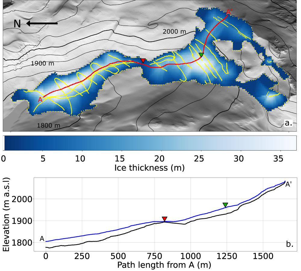
Results from the ice-penetrating radar survey show that the remaining ice at Helm Glacier is thin, with a mean and maximum ice thickness of  $13.0\,\pm 4.5\,\mathrm{m}$ and $37.2\,\pm 4.5\,\mathrm{m}$, respectively (Fig. 3). To compare these data with modelled ice thickness from Farinotti and others (Reference Farinotti2019) and Millan and others (Reference Millan, Mouginot, Rabatel and Morlighem2022), we apply a simple glacier wide surface lowering based on WGMS (2024) data from the date that the model thickness was derived to 2024. Within the 2025 boundary, estimated mean (maximum) ice thickness from Farinotti and others (Reference Farinotti2019) is 50.8 m (85.4 m) in the year 2000. From 2000 to 2024, the cumulative glacier-wide net mass loss taken from WGMS (2024) was 39.4 m w.e. (or 46.4 m of lowering assuming a density conversion factor of 0.85 (Huss, Reference Huss2013)), which would lead to a thickness estimate of 4.4 m (39.0 m) in 2025. Using data from Millan and others (Reference Millan, Mouginot, Rabatel and Morlighem2022) yields mean (maximum) thickness 53.9 m (107.6 m) in 2017–18, and from 2018 to 2024, net mass loss taken from WGMS (2024) was 15.0 m w.e. (surface lowering of 17.6 m), leading to 2025 ice thickness estimates of 36.3 m (90.0 m).
(a) Ice thickness map from linear 2D interpolation of ice-penetrating radar data (yellow dots on glacier) overlain on hillshade of LiDAR DEM with  $50\,\mathrm{m}$ contour intervals. The ice margin (yellow dots on perimeter) is set to a zero-thickness boundary and was traced out from the hillshade of the 2025 LiDAR DEM. Red line and location triangle markers in (a) show the path of cross-section in (b). Ice and bed profile were extracted from a 2D spline interpolated map at a $1\,\mathrm{m}$ upsampled resolution.

The steepest part of the tributary has a surface slope of  $30^\circ$, with an ice thickness of $15\,\mathrm{m}$, while the thickest ice in the middle of the glacier is $37\,\mathrm{m}$ with a surface slope of $8^\circ$. Assuming a shallow ice approximation and with no basal slip (e.g. Greve and Blatter, Reference Greve and Blatter2009), we compute surface velocities for each grid cell and obtain a mean velocity of $0.12\,\mathrm{m\,a}^{-1}$ and a maximum of $2\,\mathrm{m\,a}^{-1}$. Similarly, mean annual velocities from repeat optical imagery (ITS_LIVE) show a decrease in velocity at the mean elevation of the glacier from roughly $2\,\mathrm{m\,a}^{-1}$ in 1984 to $ \lt 1\,\mathrm{m\,a}^{-1}$ in 2022 (Gardner and others, Reference Gardner, Fahnestock and Scambos2022). The resulting surface elevation changes from ice advection would therefore be an order of magnitude lower than the average observed surface elevation change, justifying the omission of ice dynamics in the surface elevation change model.
Performance of the regression model
By concatenating the data across the four year observation period to compute bulk  $\hat{\boldsymbol{\beta}}$-coefficients, the model yields a bulk $R^2$ of 0.85. $\hat{\boldsymbol{\beta}}$-values are all statistically significant at $p \lt 0.001$. Comparing the modelled versus measured yearly elevation change averaged across the glacier leads to an $R^2$ of 0.96 (Fig. S2). Applying the $\hat{\boldsymbol{\beta}}$-coefficients to each year individually, then computing the differences in modelled versus observed surface elevation change across each grid cell leads to
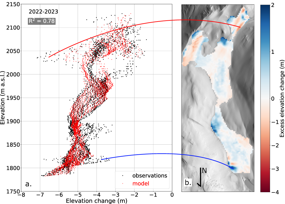
  $R^2$ values of 0.65, 0.81, 0.78 and 0.75 for the four consecutive glaciological years (2022–23 results shown in Fig. 4a, all other years shown in Fig. S3). For all years, a map of the difference between modelled and observed elevation change (Fig. 4b and Fig. S4) shows that the model is underestimating elevation change below steep valley walls where avalanching is leading to excess snow accumulation. The largest modelled underestimate of melt occurs along a steep slope near the head of the glacier, where ice is exposed early in the melt season relative to the surrounding glacier.
(a) Observed (black dots) and modelled (red dots) surface elevation change for each  $10 \times 10\,\mathrm{m}$ grid cell for the 2022–23 glaciological year. (b) Map of the observed minus modelled surface elevation change showing overestimates of surface lowering in blue with underestimates in red. Examples of points at elevation in (a) are linked to the location of the glacier in (b) for spatial context. All other years are shown in Figure S3.

A regression of the standard normal variates shows that the slope and aspect contribute to 19% and 7% of the explained variance, respectively, while snow depth accounts for 52%, PDDs account for 19% and incoming shortwave radiation accounts for only 2% of the variance. By excluding slope and aspect from the design matrix, the bulk  ${R^2}$ decreases to 0.75 while ${R^2}$ values for individual melt years drop to roughly 0.6 for all years (shown for 2022–23 in Fig. S5). Omitting both $\mathbf{SW}_{\downarrow}$ and snow depth fields from $\mathbf{X}$ can lead to reasonable estimates of elevation change for the 2020–21 and 2023–24 glaciological years, with $R^2\sim0.7$. However, $\mathbf{SW}_{\downarrow}$ needs to be included when fitting the model to the four year record to validate the high melt season of 2022–23. Similarly, snow depth needs to be included when fitting the model to the four year record to adequately model the high snow accumulation season of 2021–22. Relative to the uncertainty in ice thickness, the regression model shows little sensitivity to a change in lapse rate.
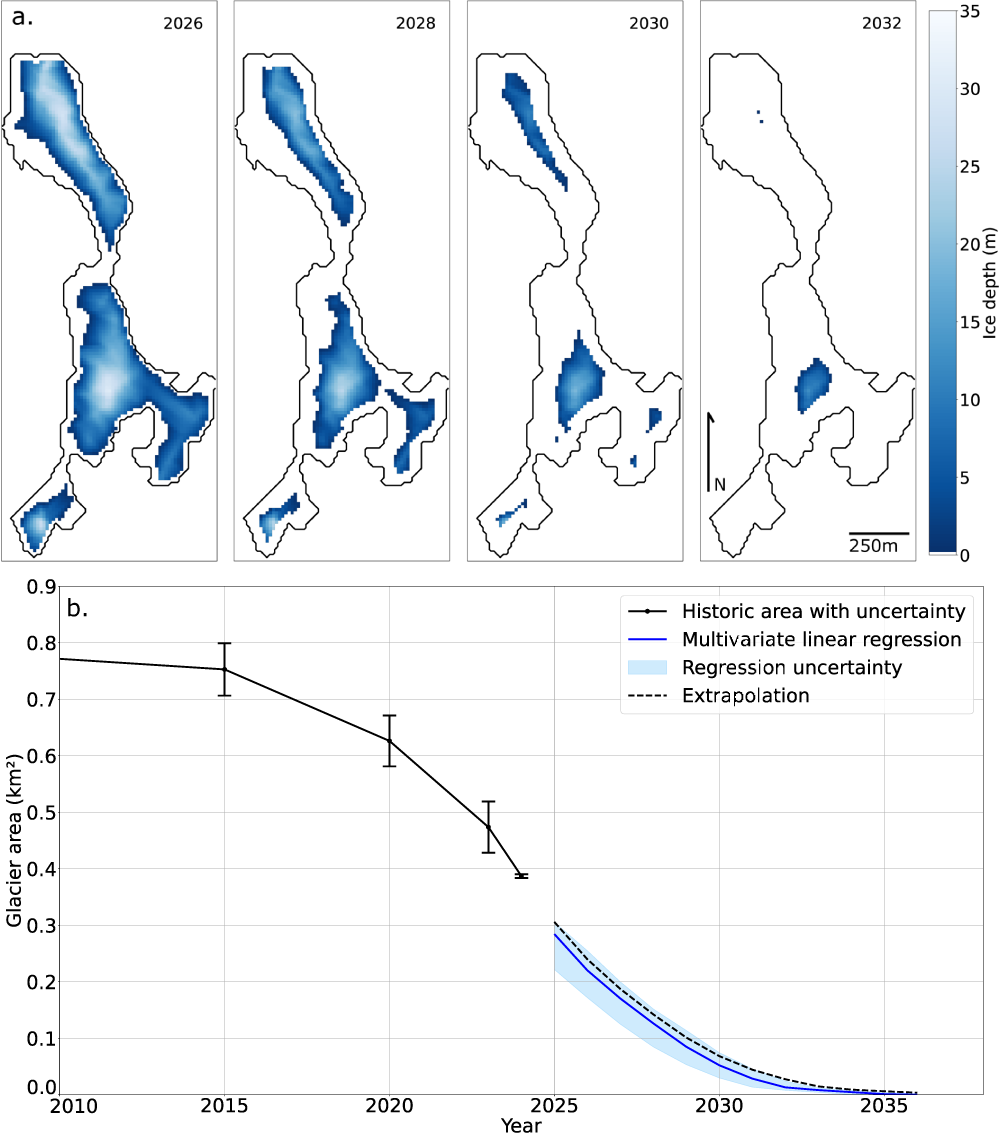
Projected ice loss
Both the simple extrapolation and the regression analysis project that Helm Glacier will fragment into ice patches less than  $0.01\,\mathrm{km}^2$ by 2035 and will no longer be classified as a glacier within a decade (Fig. 5). Projected area loss patterns are controlled predominantly by the remaining ice thickness rather than elevation, orientation and slope. With the exception of an accelerated area loss between 1985 and 1990 when thin ice melted out from shallow bed topography in the upper basin, the historic cumulative mass loss correlates very highly with the area change ( $R^2$ = 0.99, Fig. S6) with the slope of the fit being dictated by the basin geometry. By assuming that the net elevation change is from ice loss alone, we convert the modelled volume change to mass using a conversion factor of 0.917. The forward modelled cumulative mass balance—area relationship becomes concave upward as glacier area tends to zero.
(a - top panels) Glacier area and thickness forward modelled with multivariate linear regression and shown at two year increments, with 2025 outline shown in black. (b) Historic area (black line with error bars) and modelled area based on extrapolation (dashed black line) and multivariate linear regression (solid blue line), with uncertainty (light blue region) determined by  $\pm 4.5\,\mathrm{m}$ error in ice thickness.

Mass balance sensitivity
For current conditions at Helm Glacier, we compute a mass balance sensitivity to temperature as  $\mathrm{C}_\mathrm{T} = -0.58\,\mathrm{m\,w.e.\,a}^{-1}\,^\circ\,\mathrm{C}^{-1}$ while the sensitivity to snow depth is $\mathrm{C}_\mathrm{P} = 0.90\,\mathrm{m\,w.e.\,a}^{-1}\,\mathrm{m\,w.e}.^{-1}$. By normalising perturbations in temperature by the mean of the summer temperature and normalising accumulation by the mean of the winter accumulation, both from 2020 to 2024 (Fig. S7), we calculate that the glacier is roughly 12% more sensitive to changes in summer temperature than winter accumulation. Our modelled value of $\mathrm{C}_\mathrm{T} = -0.58\,\mathrm{m\,w.e.\,a}^{-1}\,^\circ\,\mathrm{C}^{-1}$ is slightly less negative than the observed mass balance temperature sensitivity of $\mathrm{C}_\mathrm{T} = -0.64\,\mathrm{m\,w.e.\,a}^{-1}\,^\circ\,\mathrm{C}^{-1}$ derived from in situ data (Fig. S8). The sensitivity analysis shows an increase in sensitivity as the temperature increases (Fig. S7). The mass balance sensitivities computed using the reference surface method or by allowing the accumulation area to grow yield the same outcome. From the modelled sensitivity of $\mathrm{C}_\mathrm{T} = -0.58\,\mathrm{m\,w.e.\,a}^{-1}\,^\circ\,\mathrm{C}^{-1}$, the mean summer temperature would need to decrease by $4.1^{\circ}\mathrm{C}$ (56%) to achieve a net-zero mass balance from the current average balance of $-2.3\,\mathrm{m}$ w.e. Similarly, the mean winter balance would need to increase by 2.55 m w.e. (138%).
Discussion
Surface elevation change
Both methods used to project the demise of Helm Glacier indicate that survival of the glacier beyond the next decade is unlikely. Extrapolating the average elevation change forward in time is more conservative than the regression model because surface parameters like slope, orientation and elevation that are updated at each yearly time step in the regression model create a positive feedback in melt rate, which is not captured with the simple extrapolation. For each melt season, modelled surface elevation change is underestimated along the glacier’s eastern margin where avalanche accumulation and shading occur. These factors are known to influence mass balance for glaciers in topographically complex settings (e.g. Olson and Rupper, Reference Olson and Rupper2019; Kneib and others, Reference Kneib2024). Elevation change is overestimated at the eastern head of the glacier where snow redistribution by wind causes a reversal of the accumulation gradient. Linear interpolation and extrapolation of snow depth measurements to the snow depth field yield the best  $R^2$ averaged across all observation periods, but in cases of extreme years for snow redistribution, a second or third-order polynomial can significantly increase the fit at high and low elevations for that year. Given that this thin glacier is strongly out of balance with the present-day climate, capturing these finer-scale patterns of accumulation and melt would not change the fate of Helm Glacier’s extinction within the decade, however. For example, slope and aspect are important for capturing across-glacier variations in melt (see Fig. S5), yet omitting these variables from the model extends the life of the glacier by only one year. Furthermore, while the simple extrapolation captures all processes not explicitly modelled in the regression, the resulting estimates of extinction timing differ only slightly between the two modelling approaches.
The linear regression model is driven by average temperatures over the past decade and an average snow depth field. As such, the forward model does not capture extreme melt events observed regionally and at Helm Glacier. Examples of events and processes that likely make our projections conservative include the extreme melt year of 2023 (Menounos and others, Reference Menounos, Huss, Marshall, Ednie, Florentine and Hartl2025), proglacial lake development leading to basal melt and calving (Carrivick and Tweed, Reference Carrivick and Tweed2013; Shugar and others, Reference Shugar2020), surface darkening and subsequent changes to albedo and radiant heat from increasing bedrock exposure (Naegeli and Huss, Reference Naegeli and Huss2017; Aubry-Wake and others, Reference Aubry-Wake, Zephir, Baraer, McKenzie and Mark2018; Reference Aubry-Wake, Bertoncini and Pomeroy2022; Marshall and Miller, Reference Marshall and Miller2020; Menounos and others, Reference Menounos, Huss, Marshall, Ednie, Florentine and Hartl2025). We have not quantified the influence of the proglacial lake on retreat rates or the effect of surface darkening and radiant bedrock heat on melt rate. Our projections do not account for small, remnant fragments of dead or debris-covered ice, which could provide important buffering capacity for ecosystem health. Though these small ice masses may exist longer than a decade, projected warming will likely melt these ice masses away by the end of the century irrespective of debris cover or shading.
Given the high correlation between glacier area and cumulative net mass balance (Fig. 2), area loss for this small glacier can validate regional approaches that seek to understand mass loss and deglaciation from area loss alone (Bahr and others, Reference Bahr, Pfeffer and Kaser2015; Bevington and Menounos, Reference Bevington and Menounos2022). The accelerated mass loss from 2011 to present (Fig. 2) is in good agreement with regional assessments of mass and area loss between 2011 and 2020 (Menounos and others, Reference Menounos2019; Hugonnet and others, Reference Hugonnet2021; Bevington and Menounos, Reference Bevington and Menounos2022) with another increase in mass loss after 2020 (Menounos and others, Reference Menounos, Huss, Marshall, Ednie, Florentine and Hartl2025). An equilibrium line rising above the head of Helm Glacier is also in agreement with regional trends of rapid equilibrium line rise that is starving these glaciers of mass (Mcgrath and others, Reference McGrath, Sass, O’Neel, Arendt and Kienholz2017; Bevington and Menounos, Reference Bevington and Menounos2025). The current fragmentation and imminent disappearance of Helm Glacier accords with a loss of 8% of glaciers throughout western Canada between 2011 and 2020, with the southern Coast Mountains being among the hardest hit (Bevington and Menounos, Reference Bevington and Menounos2022).
Our modelling results suggest that the pattern of area loss follows closely the 2025 distribution of ice thickness, largely because net mass balance is so negative. Accurate ice thickness estimates are therefore important for predicting the timing of extinction. For example, initiating a maximum ice thickness at  $39.0\,\mathrm{m}$ (derived from the Farinotti and others (Reference Farinotti2019) model) with a surface lowering rate of $2.6\,\mathrm{m a}^{-1}$ would lead to ice extinction in 14.8 years, while an initial maximum ice thickness of $90.0\,\mathrm{m}$ (derived from the Millan and others (Reference Millan, Mouginot, Rabatel and Morlighem2022) model) would lead to extinction in 34.1 years. The rate of $2.6\,\mathrm{m a}^{-1}$ represents the mean elevation change between 2020 and 2024 at the location of maximum ice thickness (green triangle marker in Fig. 3). This wide range of disappearance dates suggests that in situ thickness data are crucial for predicting the timing of extinction for small glaciers like Helm Glacier and will help to improve physically-based models of future ice evolution in western Canada.
Model parameters
For continental glaciers, temperature alone can account for over 80% of the explained variance in net mass balance (Letréguilly, Reference Letréguilly1988; Zekollari and Huybrechts, Reference Zekollari and Huybrechts2018), but as glaciers become more coastal, both temperature and precipitation are needed to explain a majority of the variance (Letréguilly, Reference Letréguilly1988; Moore and Demuth, Reference Moore and Demuth2001; Trachsel and Nesje, Reference Trachsel and Nesje2015). The continentality of Helm Glacier is  $18^{\circ}\mathrm{C}$, as computed from the 20 year mean of the difference in temperature between the warmest and coldest months. Helm Glacier is therefore transitional between continental and maritime regimes. In our regression model, we find that snow depth explains the highest variance in surface elevation change over the four year record. From the in situ mass balance record, however, the annual net balance shows positive correlation with the summer balance ( ${R^2}$ = 0.91), while the winter balance is positively correlated to the net balance, but only at ${R^2}$ = 0.41. In situ summer and winter balance records are uncorrelated.
Snow depth and temperature account for a majority of the explained variance, leaving the masked incoming shortwave radiation to account for only 2% of the explained variance despite its large contribution to melt (e.g. Munro and Marosz-Wantuch, Reference Munro and Marosz-Wantuch2009; Marshall, Reference Marshall2014). The small explained variance of  $\mathbf{SW}_{\downarrow}$ likely arises from a confounding relationship between $\mathbf{SW}_{\downarrow}$ and air temperature, which controls the timing of melt and ice exposure (Cuffey and Paterson, Reference Cuffey and Paterson2010; Marshall and Miller, Reference Marshall and Miller2020; Kinnard and others, Reference Kinnard, Larouche, Demuth and Menounos2022) and can be correlated with cloud transmittance (Pellicciotti and others, Reference Pellicciotti, Raschle, Huerlimann, Carenzo and Burlando2011). Mean glacier slope and aspect correlate with equilibrium line altitude and net mass balance at a regional scale (Rabatel and others, Reference Rabatel, Letréguilly, Dedieu and Eckert2013; Davaze and others, Reference Davaze, Rabatel, Dufour, Hugonnet and Arnaud2020). By omitting slope and aspect, we cannot capture across-glacier variations in elevation change (Fig. S5), likely because slope is a predictor for the spatial distribution of snow depth (McGrath and others, Reference McGrath2015; Pulwicki and others, Reference Pulwicki, Flowers, Radić and Bingham2018). Aspect may be affecting end-of-winter snow depth if melt is occurring prior to the survey date (Hultstrand and others, Reference Hultstrand, Fassnacht, Stednick and Hiemstra2021).
Mass balance sensitivity
At a regional scale, mass balance sensitivity depends on climatic factors such as continentality, mass balance amplitude (Hock and others, Reference Hock, De Woul, Radić and Dyurgerov2009; Anderson and Mackintosh, Reference Anderson and Mackintosh2012) and precipitation (Oerlemans and Fortuin, Reference Oerlemans and Fortuin1992), and these factors can vary seasonally depending on climate (Oerlemans and Reichert, Reference Oerlemans and Reichert2000; Hock and others, Reference Hock, De Woul, Radić and Dyurgerov2009). Mass balance temperature sensitivities for maritime-transition glaciers are generally in the range of  $-0.6 \,\mathrm{m\,w.e.\,a}^{-1}\,^\circ\,\mathrm{C}^{-1} \gt \mathrm{C}_\mathrm{T} \gt -0.9 \,\mathrm{m\,w.e.\,a}^{-1}\,^\circ\,\mathrm{C}^{-1}$ (Braithwaite and Raper, Reference Braithwaite and Raper2007; Cuffey and Paterson, Reference Cuffey and Paterson2010; Anderson and Mackintosh, Reference Anderson and Mackintosh2012; Kinnard and others, Reference Kinnard, Larouche, Demuth and Menounos2022), though again, continentality is not the sole indicator of sensitivity. Our modelled mass balance temperature sensitivity of $-0.58\,\mathrm{m\,w.e.\,a}^{-1}\,^\circ\,\mathrm{C}^{-1}$ is in close agreement with the in situ-derived value of $-0.64\,\mathrm{m\,w.e.\,a}^{-1}\,^\circ\,\mathrm{C}^{-1}$, but is slightly lower than expected given the elevation, the winter accumulation of $1.85\,\mathrm{m}$ w.e. and the continentality of $18^{\circ}\mathrm{C}$ of Helm Glacier. As the climate warms, a glacier’s mass balance sensitivity can evolve with changes in slope, aspect, elevation, debris cover (Braithwaite and Zhang, Reference Braithwaite and Zhang2000; Anderson and Mackintosh, Reference Anderson and Mackintosh2012), hypsometry (Mcgrath and others, Reference McGrath, Sass, O’Neel, Arendt and Kienholz2017; Wang and others, Reference Wang, Liu, Shangguan, Radić and Zhang2019) and albedo (Naegeli and Huss, Reference Naegeli and Huss2017; Kinnard and others, Reference Kinnard, Larouche, Demuth and Menounos2022). In our model, temperature sensitivity increases with temperature (Fig. S7), as modelled by Kinnard and others (Reference Kinnard, Larouche, Demuth and Menounos2022) and Wang and others (Reference Wang, Liu, Shangguan, Radić and Zhang2019), but we cannot parse out the confounding effects of temperature increase on geometric factors like slope, aspect, elevation and hypsometry.
The mass balance sensitivity analysis shows that Helm Glacier is currently  $4.1^{\circ}\mathrm{C}$ out of equilibrium with current conditions relative to the 2024 reference geometry. This modelled disequilibrium is close to the observed increase in mean summer temperature of $4.6^{\circ}\mathrm{C}$ from 1950 to present at the nearest ERA5-Land grid point (Fig. S9). Over the monitoring period, winter balance data from Helm Glacier show no evidence of changes in precipitation that could explain the glacier’s disequilibrium. We suggest that the glacier is likely more than $4.1^{\circ}\mathrm{C}$ out of equilibrium because mass balance sensitivity is computed from the present-day geometry, and the modelled temperature sensitivity increases over time.
Conclusion
Over the last 97 years, Helm Glacier lost 90% of its surface area, with notable accelerated area and mass loss over the past decade. We compute a mass balance sensitivity to temperature for the glacier of  $\mathrm{C}_\mathrm{T} = -0.58\,\mathrm{m\,w.e.\,a}^{-1}\,^\circ\,\mathrm{C}^{-1}$, consistent with its regional climate setting. Projected warming and the glacier’s shallow ice imply that the glacier will vanish within the next decade. For small ice masses like Helm Glacier, ice thickness is a predominant control on the timing of extinction, highlighting the importance of ice-thickness measurements. While the volume of water storage in Helm Glacier is small, the loss of this glacier will reduce the availability of long-term in situ mass balance observations from North America, which are essential for improving physically based models of glacier evolution.
Supplementary material
The supplementary material for this article can be found at https://doi.org/10.1017/aog.2026.10043.
Data availability statement
All code and data used for the regression analysis can be obtained from https://github.com/jwheelsc/helm_SEC.
Acknowledgements
We are grateful for the research supported by the National Sciences and Engineering Research Council of Canada, Tula Foundation and Natural Hazards and Climate Change Geoscience Program at the Geological Survey of Canada. We appreciate the site access granted by B.C. Parks. The ice radar survey was made possible with the help of Felix Parkinson, and mass balance monitoring was made possible with the help of Jason VanderSchoot. We thank the two anonymous reviewers who helped to improve this manuscript.
Author contributions
JWC and BM designed and co-wrote the paper. BM provided the reanalysis and LiDAR data. ME collected all in situ mass balance observations from 2019 to present and mapped historic area change. JWC collected and processed the radar data and performed the regression analysis.


 Open access