


1. Introduction
With global warming, more icebergs are breaking off from Antarctica, accelerating sea level rise (Scambos et al. Reference Scambos2017). Additionally, melting icebergs and sea ice floes also contribute significantly to climate and environment change, including freshwater supply (Huppert & Turner Reference Huppert and Turner1978), biological productivity (Wadham et al. Reference Wadham, Hawkings, Tarasov, Gregoire, Spencer, Gutjahr, Ridgwell and Kohfeld2019) and carbon sequestration (Duprat, Bigg & Wilton Reference Duprat, Bigg and Wilton2016), making the understanding of iceberg melting rates crucial for comprehending the interplay between icebergs and the climate (Cenedese & Straneo Reference Cenedese and Straneo2023). To describe the melt rate of icebergs, different parametrization models are proposed, such as employing empirical relations for turbulent heat transfer over a flat plate to predict iceberg melt rates (Weeks & Campbell Reference Weeks and Campbell1973), considering meltwater-plume effect on the melt rate with ambient flows (FitzMaurice, Cenedese & Straneo Reference FitzMaurice, Cenedese and Straneo2017), and coupling effects of turbulence, buoyant convection and waves (Martin & Adcroft Reference Martin and Adcroft2010).
Various lab experiments and direct numerical simulations have been conducted to investigate the interaction between ice melting and ambient flow in the laboratory scale, including ice melting in still and flowing water (Dumore, Merk & Prins Reference Dumore, Merk and Prins1953; Vanier & Tien Reference Vanier and Tien1970; Hao & Tao Reference Hao and Tao2002; Hester et al. Reference Hester, McConnochie, Cenedese, Couston and Vasil2021; Weady et al. Reference Weady, Tong, Zidovska and Ristroph2022), in Rayleigh–Bénard convection (Davis, Müller & Dietsche Reference Davis, Müller and Dietsche1984; Dietsche & Müller Reference Dietsche and Müller1985; Esfahani et al. Reference Esfahani, Hirata, Berti and Calzavarini2018; Favier, Purseed & Duchemin Reference Favier, Purseed and Duchemin2019; Yang et al. Reference Yang, Howland, Liu, Verzicco and Lohse2023b), which involves a plate being heated from below and a plate being cooled from above (Lohse & Xia Reference Lohse and Xia2010; Ecke & Shishkina Reference Ecke and Shishkina2023), and in vertical convection (Wang et al. Reference Wang, Jiang, Du, Sun and Calzavarini2021c; Yang et al. Reference Yang, Chong, Liu, Verzicco and Lohse2022). The density anomaly effect in freshwater, combined with inclination, causes distinct flow regimes and ice melting morphology under different temperatures, which has been comprehensively investigated by Wang, Calzavarini & Sun (Reference Wang, Calzavarini and Sun2021a), Wang et al. (Reference Wang, Calzavarini, Sun and Toschi2021b,Reference Wang, Jiang, Du, Sun and Calzavarinic). Salinity results in even more complex mushy layer structures (Worster Reference Worster1997), where convection also occurs (Du et al. Reference Du, Wang, Jiang, Calzavarini and Sun2023). These studies highlight the complex interplay between ice melting and ambient flow, leading to distinct ice morphologies and melt rates.
Icebergs and ice floes exhibit considerable variations in shape and size (Gherardi & Lagomarsino Reference Gherardi and Lagomarsino2015), with horizontal extents ranging from a few metres to several hundred kilometres. Despite extensive research on iceberg melt rates using models, experiments and simulations, the potential effects of the aspect ratio on the melt rate have not received much attention. One of the experimental results is that the overall melt rate strongly depends on the aspect ratio (Hester et al. Reference Hester, McConnochie, Cenedese, Couston and Vasil2021; Cenedese & Straneo Reference Cenedese and Straneo2023), which is also the motivation for our study on the aspect ratio effect on the melt rate.
Further theoretical understanding on the melting of solid objects in fluid flow can be gained from the analogy with dissolution or erosion processes. Whereas the ablation rate of a melting object is determined by the temperature gradient at the liquid–solid boundary, for dissolution this is instead the gradient of solute concentration, and for erosion it is the shear stress at the boundary. From this perspective, the underlying physics of melting and dissolution are identical, and the Reynolds analogy for passive scalar transport can be used to also draw comparisons with erosion. Ristroph et al. (Reference Ristroph, Moore, Childress, Shelley and Zhang2012) performed experiments of an erodible sphere in a uniform flow and use a simple boundary-layer model to describe the resulting self-similar shape. Moore et al. (Reference Moore, Ristroph, Childress, Zhang and Shelley2013) extended this work with further experiments and quasistatic simulations to describe how other initial shapes, including ellipses, evolve towards a self-similar shape. For dissolving objects, Huang, Moore & Ristroph (Reference Huang, Moore and Ristroph2015) use a similar boundary layer approach to describe the dissolution rate and resulting dynamical shapes. Although this series of work has made great progress in understanding the ablation rate scalings and shape evolution, the effect of the initial aspect ratio on the time taken for the object to vanish has not yet been considered. We note that a difference between melting and dissolution is the very different Prandtl respective Schmidt number, with the latter one for dissolution typically being more than two orders of magnitude larger.
In this study, we investigate the influence of the ice shape (ellipse aspect ratio) on melt rates through numerical simulations and theoretical analysis in an idealized setting. We focus on the scenario of ice melting in a uniform flow, as detailed in § 2, and neglect buoyancy effects and basal melting due to our focus on the top view of the melting process, distinguishing our work from previous studies (Couston et al. Reference Couston, Hester, Favier, Taylor, Holland and Jenkins2021; Hester et al. Reference Hester, McConnochie, Cenedese, Couston and Vasil2021). Our aim is to understand how the aspect ratio affects ice melt rates by conducting a series of numerical simulations in a simplified system as a fundamental problem. Our findings reveal that the aspect ratio plays a crucial role in the melting process, leading to substantial variations in melt rates. We further propose a theoretical model for the dependence of melt rates on the control parameters that agrees well with the simulation results. In this model, two contributions to the total melt rate are distinguished – surface contact-induced melt and advective flow-induced melt. The observed strong aspect ratio dependence can be quantitatively understood.
2. Numerical method and set-up
We numerically integrate the velocity field  $\boldsymbol {u}$ and the temperature field $\theta$ according to the Navier–Stokes equations, neglecting the effect of buoyancy induced by temperature differences. The melting process is modelled by the phase-field method, which has been widely used in previous studies (Favier et al. Reference Favier, Purseed and Duchemin2019; Couston et al. Reference Couston, Hester, Favier, Taylor, Holland and Jenkins2021; Hester et al. Reference Hester, McConnochie, Cenedese, Couston and Vasil2021; Yang et al. Reference Yang, Chong, Liu, Verzicco and Lohse2022, Reference Yang, Howland, Liu, Verzicco and Lohse2023b). In this technique, the phase-field variable $\phi$ is integrated in time and space and smoothly transitions from a value of $1$ in the solid to a value of $0$ in the liquid. The equations are non-dimensionalized by inflow speed $U_0$ as the velocity scale, ice effective diameter $D$ as the length scale, and the temperature difference between the ambient flow and the ice $T_0$ as the temperature scale. The non-dimensionalized quantities include three velocity components $u_i$ with $i=1,2,3$, the pressure $p$, the temperature $\theta$ and the phase-field scalar $\phi$. The dimensionless governing equations read
 $$\begin{gather} \boldsymbol{\nabla} \boldsymbol{\cdot} \boldsymbol{u}=0, \end{gather}$$
 $$\begin{gather}\partial_t \boldsymbol{u}+\boldsymbol{\nabla} \boldsymbol{\cdot} (\boldsymbol{u} \boldsymbol{u})={-}\boldsymbol{\nabla} p+\frac{1}{Re}\nabla^2 \boldsymbol{u}, \end{gather}$$
 $$\begin{gather}\partial_t \theta+\boldsymbol{\nabla} \boldsymbol{\cdot} (\boldsymbol{u} \theta)=\frac{1}{{RePr}} \nabla^2 \theta+S t \partial_t \phi, \end{gather}$$
 $$\begin{gather}\frac{\partial \phi}{\partial t}=\frac{6}{5 S t C {{RePr}}}\left[\nabla^2 \phi-\frac{1}{\beta^2} \phi(1-\phi)(1-2 \phi+C \theta)\right], \end{gather}$$
where  $\beta$ is the diffusive interface thickness, which is typically set to be the mean grid spacing. The control parameters of the system are the Reynolds number $Re$, which is the dimensionless flow strength, the Prandtl number $Pr$, which is the ratio between kinematic viscosity $\nu$ and thermal diffusivity $\kappa$, and the Stefan number $St$, which is the ratio between latent heat and sensible heat, and the aspect ratio of the initial ice shape $\gamma$, which is defined as the ratio of its width and length and will be the focus of this paper:
 \begin{equation} Re=\frac{U_0D}{\nu},\quad Pr=\frac{\nu}{\kappa},\quad St=\frac{\mathcal{L}}{c_p\varDelta T},\quad \gamma=\frac{l_w}{l_l}. \end{equation}
Here,  $U_0$ is the inflow velocity, $l_w$ and $l_l$ are the initial width and length of the ice shape (shown in figure 1b), $\mathcal {L}$ is the latent heat, $c_p$ is the specific heat capacity, $\varDelta T=T_0-T_i$ is the temperature difference between inflow temperature $T_0$ and the initial ice temperature $T_i$. Due to the large parameter space, some of the control parameters have to be fixed in order to make the study feasible. For the time being, we fix $Pr=7$ and $St=4$ as the values for water at $20\,^\circ {\rm C}$, unless specified otherwise, and $T_i=0\,^\circ {\rm C}$, the same as the melting temperature. Varying $T_i$ presumably also affects the melting process as the temperature conduction inside the solid also plays a role, which is worth further exploration. Later we also investigate the effect of $Pr$ and $St$ independently. Our simulations cover a parameter range of $0\le Re\le 10^3$ ( $Re=10^3$ corresponds to flow speed $U=5\ {\rm cm}\ {\rm s}^{-1}$ and ice diameter $D=2$ cm) and $0.1 \le \gamma \le 2.25$. Here $C$ is the phase mobility parameters related to the Gibbs–Thompson relation. We choose $C = 1$, which may overestimate the Gibbs-Thomson effect for high curvature. Therefore we avoid too extreme values of $\gamma$, where the high curvature regions might be inaccurate. We further impose a direct forcing of the velocity to zero for $\phi >0.9$, preventing spurious motions inside the solid phase (Howland Reference Howland2022). More details can be found in previous studies (Hester et al. Reference Hester, Couston, Favier, Burns and Vasil2020; Yang et al. Reference Yang, Howland, Liu, Verzicco and Lohse2023b). Simulations are performed using the second-order staggered finite difference code AFiD, which has been extensively validated and used to study a wide range of turbulent flow problems (Ostilla-Mónico et al. Reference Ostilla-Mónico, Yang, Van Der Poel, Lohse and Verzicco2015; Yang, Verzicco & Lohse Reference Yang, Verzicco and Lohse2016; Liu et al. Reference Liu, Chong, Yang, Verzicco and Lohse2022), including phase-change problems (Yang et al. Reference Yang, Chong, Liu, Verzicco and Lohse2022, Reference Yang, Howland, Liu, Verzicco and Lohse2023b). The phase-field method is applied to model the phase-change process, which has been widely used in previous studies (Favier et al. Reference Favier, Purseed and Duchemin2019; Couston et al. Reference Couston, Hester, Favier, Taylor, Holland and Jenkins2021; Hester et al. Reference Hester, McConnochie, Cenedese, Couston and Vasil2021; Ravichandran & Wettlaufer Reference Ravichandran and Wettlaufer2021; Yang et al. Reference Yang, Howland, Liu, Verzicco and Lohse2023b).
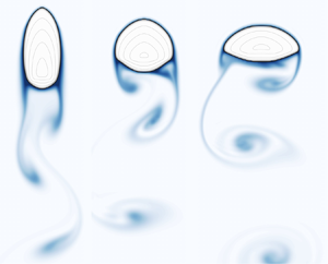
(a) An illustration of the set-up for ice melting in flowing water. The inflow is set at the left boundary with unidirectional velocity  $U_0$ and uniform temperature $T_0$. (b) Zoomed-in view of the ice object. Here $l_w$ and $l_l$ represent the width and the length of the object, respectively. Panels (c–f) represent the snapshots of the temperature field of ice melting in flowing water with different aspect ratios $\gamma$, namely (c) $\gamma =0.25$, (d) $0.44$, (e) $1$ and (f) $2.25$. The corresponding movies are shown as supplementary movies and are available at https://doi.org/10.1017/jfm.2023.1080. Panels (g–j) show the snapshots of $\partial \phi /\partial t$ (see text for more details), corresponding to the cases in (c–f). The colour represents the local melt rate over the surface at different times. Also, the corresponding plot of the shift distance $\tilde {D}_x$ (normalized by corresponding $l_l$) of the centroids as a function of the dimensionless time is given. The mass loss rate $\dot {m}$, normalized $\partial \phi /\partial t$, is colour-coded.

The flow is confined vertically by two parallel boundaries with free-slip boundary conditions for the velocity and adiabatic for the temperature (see figure 1a). In the simulations, we prescribe an ice object with area  $A_0$ and effective diameter $D=2\sqrt {A_0/{\rm \pi} }$ in a domain of length $L=20D$ and width $W_z=5D$. Both two-dimensional (2-D) ( $L/W_z=4$) and three-dimensional (3-D) simulations ( $L/W_z=L/W_x=4$) are conducted. The long and short axis lengths of the ellipse are $l_l=D/\sqrt {\gamma }$ and $l_w=D\sqrt {\gamma }$, respectively. Note that the finite cross-stream dimension of the computation domain could in principle lead to blockage effects. To ensure that this does not affect our results, we performed a test for circle shapes at $Re=400$ with different $W_z$, which produced a convergent melt rate at $W_z=5D$. Initially, the simulations are run with the ice object fixed at zero velocity and $\theta _i=0$, and the melting process is turned off until the flow reaches the fully developed stage, then we turn on the melting process. The velocity and temperature at the left and right boundary are set as uniform $U_0$ and $T_0$ by a penalty force. The initial temperature of the ice is set as the melting temperature $\theta _i=0$, and the ambient fluid is set as the inflow temperature $\theta =1$. The position of the ice front is described as isocontour $\phi =1/2$ as time evolves. Grid convergence tests are shown in figure 2.
Resolution convergence test. (a) The normalized area as a function of dimensionless time for different resolutions at  $Re=400$. (b) The contour plots of the ice surface at $t=8t_0$ (grey dashed line in (a)). (c) Calculated $t_f$ as a function of the grid resolution. The dashed line shows the value of $t_f$ for the highest resolution we run. Based on this, our final choice of the resolution N of the cross-section length for $Re=400$ is $N=576$. (d) The relative convergence test. The $y$-axis is the relative error $|t_f-t_{f_0}|/t_{f_0}$ where $t_{f_0}$ is the $t_f$ for the highest resolution. The dashed lines represent the linear and quadratic relations.

3. Shape evolution and melt-rate dependence on parameters
We first investigate the evolution of ice shapes, which depends on the initial shape and the flow rate. Temperature fields under different initial shapes for a fixed area are shown in figure 1(c–f) ( $\gamma$ increases from (c) to (f)). From the temperature field, one can see the complex interaction between melting and detaching wake vortices. The ice has distinct front and back shapes – ice at the back is more deformed than at the front, due to the detaching vortices in the wake flow, which induce reduced and non-uniform heat flux.
To study the local melt rate at the ice front, we further plot  $\partial \phi /\partial t$ in figure 1(g–j), whose value is zero in the solid and liquid phases. At the solid–liquid interface, its value provides insight into the local melt rate. It reveals that two parts of the ice melt faster (in reddish colour): the front due to inflow, and the back due to wake flow. This melting characteristic is similar to that of dissolution (Ristroph et al. Reference Ristroph, Moore, Childress, Shelley and Zhang2012; Huang et al. Reference Huang, Moore and Ristroph2015) and to what was formed in previous experiments on melting spheres (Hao & Tao Reference Hao and Tao2002), where the front tends to melt faster than the back. This occurs because the liquid at the back of the solid is cooler than at the front due to mixing induced by the wake. We investigate the front-to-back asymmetry in the melting by plotting the distance of the ice centroid from its initial position over time in figure 1(g–j). For small $\gamma$, we observe a significant shift of the centroid to the back, while for large $\gamma$, the larger cross-section results in stronger detaching flow, which enhances melting at the back and thus prevents a significant movement of the centroid (see figure 1f). As melting progresses, the front of the shape remains rounded, and different back shapes are obtained for different $\gamma$. These shapes can be attributed to the presence of the detaching vortices, whose shedding occurs in an oscillating manner at the top and bottom of the body. As a result, melting is favoured at the top and bottom, creating a wedge-like shape. It is also interesting to note that earlier works emphasized that the front shape of eroding/dissolving bodies converges to a terminal form (Ristroph et al. Reference Ristroph, Moore, Childress, Shelley and Zhang2012; Huang et al. Reference Huang, Moore and Ristroph2015). Here we observed that slender bodies are blunted and blunt bodies are made slender. The front shapes of different bodies become similar as they melt, but they completely melt before the stage where they may converge to a terminal form.
The complicated ice–water interaction affects not only the melting shape but also the melt rate. Figure 3(a) shows the normalized total area change over time for different aspect ratio  $\gamma$. For increasing $\gamma$, the melt curves exhibit a non-monotonic trend, with the melt rate first decreasing and then increasing. We measure the time taken for the ice to completely melt as $t_f$, and take $\bar{f}=1/t_f$ to be the mean melt rate. Figure 3(b) shows the normalized melt rate $\bar{f}/f_0$ as a function of $\gamma$ for different $Re$, where $f_0(Re)$ is the mean melt rate for the circles ( $\gamma =1$). Here, the same trend is observed, and $\bar {f}$ depends not only on $\gamma$ but also on $Re$. In the absence of flow ( $Re=0$), the minimum melt rate occurs at the optimal aspect ratio $\gamma _{min}=1$ for a circle shape. As $Re$ increases, $\gamma _{min}$ decreases until it converges to approximately $\gamma _{min}\approx 0.5$. The same trend is also observed for 3-D simulations of a cylinder with the cross-section of different aspect ratios.
(a) The area  $A$ normalized $A_0$ as function of time normalized by $t_0=D/U_0$ for different $\gamma$ and fixed $Re=10^3$, $Pr=7$ and $St=4$. (b) Overall melt rate $\bar {f}/f_0$ (from initial to complete melt), normalized by the overall melt rate $f_0$ at $\gamma =1$, as a function of $\gamma$ for different $Re$. The inset image shows the snapshots of temperature fields for 3-D simulation results ( $Re=10^3$). The dashed line is the theoretical curve from (4.6), which is expected to hold for larger $Re$.
$Re$.

Our findings demonstrate that ice with an elliptical shape (when the long axis is aligned with the flow direction) can melt up to 10 % slower than a circle shape when exposed to flowing water. This previously neglected shape factor may have implications for accurately estimating the melt rate of icebergs in previous models that neglected it (Weeks & Campbell Reference Weeks and Campbell1973; Martin & Adcroft Reference Martin and Adcroft2010; FitzMaurice et al. Reference FitzMaurice, Cenedese and Straneo2017). The non-intuitive nature of this phenomenon raises a further question about its physical mechanism.
4. Theoretical model for the melt rate
To quantitatively explain the result, we follow the same approach as used by Ristroph et al. (Reference Ristroph, Moore, Childress, Shelley and Zhang2012) and Huang et al. (Reference Huang, Moore and Ristroph2015) for eroding or dissolving bodies and consider the total ice mass budget for the melting process:
 \begin{equation} \frac{{\rm d} A(t)}{{\rm d} t}=P(\gamma,t)v_n,\end{equation}
where  $P(\gamma,t)$ is the perimeter of the ice (for 2-D), and $v_n(t)$ is the surface-averaged melt speed. Assuming the elliptical shape is not significantly changing with time (i.e. $\gamma (t)\approx \gamma (t=0)=\gamma$), we have the expression for the ellipse perimeter from the elliptic integral:
 \begin{equation} P(\gamma,t)=2\sqrt{\frac{A(t)}{{\rm \pi}\gamma}}\int^{2{\rm \pi}}_0\sqrt{1-(1-\gamma^2) \sin^2\alpha}\, {\rm d} \alpha,\end{equation}
where  $\alpha$ is the angle. Here $v_n(t)$ would be uniform everywhere in the absence of flow. The presence of a flow around the body increases the temperature gradient at the ice front which enhances the heat transfer and also makes $v_n(t)$ non-uniform as $v_n(\alpha,t)$. The flow creates a viscous boundary layer and a thermal boundary layer, respectively of thicknesses $\delta _\nu$ and $\delta _\theta$. The width ratio of the boundary layers is given by the Prandtl number; $Pr=\nu /\kappa =7$ in our case implies $\delta _v>\delta _\theta$, as illustrated in figure 4(a,b). In order to understand the coupling between the shape of the object and the flow around it, we consider the Stefan boundary condition, i.e. the (dimensionless) surface-averaged melt speed $\tilde {v}_n$ is related to the surface-averaged heat flux $\overline {Nu}$:
 \begin{equation} \tilde{v}_n=\frac{v_n}{U_0}={-}\frac{1}{U_0}\frac{\kappa c_p}{\mathcal{L}} \frac{\partial T}{\partial n}=\frac{\overline{Nu}}{StPrReA^{1/2}},\end{equation}
where we can use the relation from the well-known scaling of thermal boundary-layer thickness (Meksyn Reference Meksyn1961; Grossmann & Lohse Reference Grossmann and Lohse2004) for the laminar boundary layer:
 \begin{equation} \overline{Nu}\sim\delta_\theta^{{-}1}\sim Re_{l_w}^{1/2}Pr^{1/3}/C(Pr),\end{equation}
with  $Re_{l_w}=l_w U/\nu$ the Reynolds number defined by the cross-section length $l_w=2\sqrt {\gamma A/{\rm \pi} }$, $C(Pr)$ is an infinite alternating series given in Meksyn (Reference Meksyn1961). In the limit of large $Pr$, the series for $C(Pr)$ will converge to $C(Pr) = 1$. By substituting equations (4.2) and (4.3) into (4.1), we obtain an ordinary differential equation which is easily solved, with the result
 $$\begin{gather} A(t)=A_0\left(1-\frac{t}{t_f}\right)^{{4}/{3}}, \end{gather}$$
 $$\begin{gather}\ t_f^{{-}1}\sim P(\gamma)\gamma^{1/4}\frac{Pr^{{-}2/3}}{C(Pr)}St^{{-}1}. \end{gather}$$
The  $4/3$ scaling of (4.5) is identical to that derived by Ristroph et al. (Reference Ristroph, Moore, Childress, Shelley and Zhang2012) and Moore et al. (Reference Moore, Ristroph, Childress, Zhang and Shelley2013) for eroding bodies, and the time to fully melt (4.6) is similar to the expression obtained by Huang et al. (Reference Huang, Moore and Ristroph2015) in the case of dissolution, though there Prandtl/Schmidt number is more than two orders of magnitude larger. The additional novelty of (4.6) is in the dependence on the aspect ratio $\gamma$, which arises from including such dependence in the Reynolds number used in (4.4). This dependence is the focus of this work.
(a). A schematic of the flow and temperature fields for different  $\gamma$. The steady outer flow consists of warm water, while the attached flow near the body forms a boundary layer (dashed line) containing the melted fluid. It also shows that the separation point of flow moves downstream as $\gamma$ decreases. (b) Zoomed-in view of the velocity and temperature boundary layers, the former defined by the velocity and the latter by the temperature gradient. (c) The theoretical curve from (4.6), including $P(\gamma )$, $\epsilon ^{1/4}$ and $P(\gamma )\gamma ^{1/4}$ as a function of $\gamma$. Here, $Pr=7$, $St=4$.

From (4.6) the overall melt rate  $\bar {f}$ depends on $\gamma$ as $\bar {f}=t_f^{-1}\sim P(\gamma )\gamma ^{1/4}$, where $\gamma ^{1/4}$ originates from the scaling of $\overline {Nu}$, representing the advective flow-induced melt, and $P(\gamma )$ represents the surface contact-induced melt. The contributions of $P(\gamma )$ and $\gamma ^{1/4}$ are both presented in figure 4(b), with $P(\gamma )$ exhibiting a symmetric curve as a function of $\gamma$ with a minimum at $\gamma =1$, which represents melting without flow. In contrast, $\gamma ^{1/4}$ displays a monotonic increase in melt rate, indicating that ambient flow enhances melt rate. The overall melt rate $\bar {f}\sim P(\gamma )\gamma ^{1/4}$ has a non-monotonic trend with $\gamma$, with a minimum at $\gamma _{{min,theory}}=0.48$ (which is essentially the same as the value $\gamma _{{min,sim}} \simeq 0.5$ observed by our numerical simulations). Figure 3(b) shows the total melt-rate curve, which agrees well with the numerical results obtained at high $Re$ in our numerical results. For relatively low $Re$ and even $Re=0$, the advective flow is weak, meaning $\overline {Nu}$ is close to $1$, instead of satisfying the boundary-layer relation (4.4).
In summary, the non-monotonic relation and shift of the minimum melt-rate point are physically explained by the combined contributions from the melt driven by surface contact and the melt driven by the advective flow. The former is related to the surface area, with the minimum at  $\gamma =1$, while the latter is driven by the ambient flow, leading to a monotonic increase in melt rate with increasing $\gamma$. We confirmed that the assumption of a fixed shape as the ice melts is valid by comparing the measured and calculated perimeters from (4.2) in figure 5(a). The ratio remains close to $1$, except for large $\gamma$, which is attributed to the strong wake flow (see figure 1f). The deviation of the assumption at large $\gamma$ also explains the deviation in figure 3(b) at large $\gamma$.
(a) The ratio between the measured perimeter from simulations and the ideal elliptical perimeter from (4.2) for varying  $\gamma$ at $Re=400$. The ratio close to $1$ means that our assumption is valid. (b) The normalized area $A/A_0$ as a function $1-t/t_f$ for varying $\gamma$ at $Re=400$. All curves follow the $4/3$ scaling as theoretically derived in (4.5). (c) The compensated plot of the normalized area $A/A_0(1-t/t_f)^{-4/3}$ as a function $1-t/t_f$ for varying $\gamma$ at $Re=400$. (d) The melt rate as a function of $St$ for fixed $\gamma =1$. The dashed grey line represents $\bar {f}\sim St^{-1}$. (e) The melt rate as a function of $Pr$ for fixed $\gamma =1$. The dashed grey line represents $\bar {f}\sim Pr^{-2/3}/C(Pr)$.

5. Melt rate scalings – comparison of theory and numerical result
In order to test the scaling law  $A(t)\sim (1-t/t_f)^{4/3}$ derived in the previous section, we conducted simulations with varying $\gamma$ and fixed $Re=10^3$, $Pr=7$ and $St=4$. The evolution of the area of the object is depicted in figure 5(b), along with the scaling law given by (4.5). The trends from simulations for different $\gamma$ all follow the $4/3$ scaling, in agreement with the theoretical result. Our findings demonstrate that regardless of the different physical mechanisms causing the body to ablate, whether it be through erosion (Ristroph et al. Reference Ristroph, Moore, Childress, Shelley and Zhang2012), dissolution (Huang et al. Reference Huang, Moore and Ristroph2015) or melting, the scaling laws associated with the vanishing of the body are analogous.
Besides the dependence of the melt rate on  $\gamma$, we can also obtain the scaling dependence of the melt rate on $Pr$ and $St$ from (4.6). To validate this scaling law, we performed simulations with varying $St$ in figure 5(c) while keeping $\gamma$ fixed at $1$ and $Pr$ fixed at $7$. At large $St$ (relevant for icebergs melting in cold water), the melt rate from simulation results follows $\bar {f}\sim St^{-1}$, which is consistent with the scaling law from (4.6). At small $St$, the scaling deviates from $St^{-1}$. It could be because ice melts so fast that the melted fluid is still surrounding the ice, regardless of the ambient flow. This trend has also been observed in the study of melting in convection (Favier et al. Reference Favier, Purseed and Duchemin2019). Another possible reason is that as the solid melts and the size decreases, the curvature term affects the surface melt temperature, which can cause heat diffusion inside the solid and affect the heat flux, thus the departure from the $St^{-1}$ scaling. It has a more obvious effect for low $St$ because the melt is so fast that the size of the solid quickly decreases. However, in most of our simulations and most of realistic cases, e.g. ice melting, we have $St>1$, where $St^{-1}$ scaling agrees well. We also conducted simulations with varying $Pr$ in figure 5(c) while keeping $\gamma$ fixed as $1$ and $St$ fixed as $4$. The simulation results follow $\bar {f}\sim Pr^{-2/3}/C(Pr)$ from (4.6), implying a simplified scaling $\bar {f}\sim Pr^{-2/3}$ for large $Pr$, which agrees with our results. In brief, our simulation results for varying $St$ and $Pr$ both show good agreement with the scaling law derived in (4.6).
6. Conclusions and outlook
Through a combination of simulations and theoretical modelling, we conducted a comprehensive investigation of the melting dynamics of a disk/elliptical shape of ice immersed in a uniform flow, taking into account the coupled dynamics between flow and ice melting for various initial shapes. Our results demonstrate that in the presence of an incoming flow, the front keeps a rounded shape during the melting process, while the back of the ice exhibits different shapes depending on the initial shape. Our simulations reveal that the presence of detaching vortices behind the ice plays a crucial role in shaping the melting pattern of the object.
Furthermore, we observed that the shape of the ice also has a significant effect on the melt rate. In the absence of flow, the circular shape ( $\gamma =1$) melts more slowly than other elliptical shapes $\gamma \neq 1$. However, in the presence of an external flow, some elliptic cylindrical bodies ( $\gamma <1$) melt less rapidly than circular cylinders with the same volume. This optimal aspect ratio depends on the flow strength, represented by $Re$. Our physical understanding of this dependence of the melt rate on the initial aspect ratio comes from the combined contributions from both the surface-contact-induced melt ( $\sim P(\gamma )$) and the advective-flow-induced melt ( $\sim \gamma ^{1/4}$). By assuming a laminar boundary layer, we obtained a model ((4.5) and (4.6)), accurately predicting the overall melt rate and its scaling as a function of $\gamma$, $Pr$ and $St$. Note that the Gibbs–Thomson curvature term is constantly increasing over time as the ice melts, which may affect the estimate of $t_f$. But the trend of the melt rate dependence on $\gamma$ should be the same, as we consider the relative melt rate for different $\gamma$ compared with the disk. Our findings provide insight into the rich coupling dynamics between the ice–water interface and ambient flows and demonstrate the importance of considering ice shape in predicting melting rates, advancing the understanding of previous studies (Hao & Tao Reference Hao and Tao2002; Ristroph et al. Reference Ristroph, Moore, Childress, Shelley and Zhang2012; Moore et al. Reference Moore, Ristroph, Childress, Zhang and Shelley2013; Huang et al. Reference Huang, Moore and Ristroph2015). Though the present setting has many idealizations, we believe there is scientific importance for our study as an interesting and non-intuitive fundamental finding that the circle does not always melt the slowest. More factors will be gradually added, such as the gravity effect, salinity effect, and their combinations, which we will investigate in the next step.
Beyond the elliptical shape we explored in this study, it would be interesting to explore a wider range of shapes to find the optimal one. The results could be sensitive to the initial shape since flow separation is an important factor. From the shape progression images of figure 1, the fastest melt rates occur in the front where the boundary-layer flow is attached to the body, while the back region in the separated wake melts more slowly. Therefore, a shape that triggers separation earlier without strongly changing the cross-section could melt more slowly. The approach employed in this study, which combines fully resolved direct numerical simulations and theoretical explanations, offers the possibility to explain other phase-change problems coupled with advective flows. We caution that our findings reveal only a subset of the numerous factors that influence the ice–water system dynamics. In future investigations, it would be worthwhile to further explore additional factors such as the buoyancy force (Favier et al. Reference Favier, Purseed and Duchemin2019; Couston et al. Reference Couston, Hester, Favier, Taylor, Holland and Jenkins2021; Wang et al. Reference Wang, Calzavarini, Sun and Toschi2021b; Yang et al. Reference Yang, Howland, Liu, Verzicco and Lohse2023b), melting near sidewalls or basal walls in the presence of ambient flow, and the effect of dissolved salt (Huppert & Turner Reference Huppert and Turner1978; Du et al. Reference Du, Wang, Jiang, Calzavarini and Sun2023; Yang et al. Reference Yang, Howland, Liu, Verzicco and Lohse2023a). These topics have significant relevance to the modelling of geophysical and climatological large-scale processes. Additionally, we plan to investigate the interaction between the motion of solid objects and phase change, as this holds significant potential for further exploration since icebergs can move and rotate.
Supplementary movies
Supplementary movies are available at https://doi.org/10.1017/jfm.2023.1080.
Acknowledgements
We acknowledge PRACE for awarding us access to MareNostrum in Spain at the Barcelona Computing Center (BSC) under the project 2020235589 and project 2021250115 and the Netherlands Center for Multiscale Catalytic Energy Conversion (MCEC). We also acknowledge the support by the Priority Programme SPP 1881 Turbulent Superstructures of the Deutsche Forschungsgemeinschaf and the ERC-Advanced Grant under project ‘MultiMelt’ with no. 101094492.
Funding
This research was supported in part by the National Science Foundation under grant no. NSF PHY-1748958.
Declaration of interests
The authors report no conflict of interest.


 Open access