


1. Introduction
Rigid robots depend on simulation as an inner loop of modeling, control, and computational design algorithms. Tremendous effort has gone into ensuring such simulators are fast, robust, and accurate, thus enabling these downstream applications. What is more, many of these simulators are differentiable, meaning gradients can be computed with respect to most, if not all aspects of the physical rigid body system. Such differentiability has unlocked powerful applications in robotics, such as trajectory optimization (which leverages state-of-the-art gradient-based numerical optimizers), optimal closed-loop control strategies, gradient-based system identification, and parametric automated design. By comparison, the landscape of simulators for soft robotic simulation is paltry. Unlike rigid body simulators which need only simulate a small number of rigid objects (usually tens to a few hundreds) with relatively few degrees of freedom (DoFs) and sparse contact, soft robot simulators strive to simulate elastic continuum structures which are, by nature, infinite dimensional. In order to accurately simulate these structures, these infinite dimensional structures must be discretized into a large number of finite primitives, often in the tens of thousands range or higher, with dense, complex contact. Computing gradients of such a system is even more complex, making computational modeling, control, and design of soft robots vastly underexplored compared to their rigid brethren.
In order to address shortcomings in the space of computational modeling of soft robots, Hu et al. [Reference Hu, Liu, Spielberg, Tenenbaum, Freeman, Wu, Rus and Matusik1] presented ChainQueen, an open-source, fully differentiable soft robot simulator. ChainQueen is based off the material point method (MPM) [Reference Sulsky, Zhou and Schreyer2], a hybrid Lagrangian–Eulerian method that uses both particles and a background grid for simulation. ChainQueen is fast, fully differentiable (even in the presence of complex contact), and allows for highly accurate and precise simulation. Because both simulation and gradient computation are computed on the graphics processing unit (GPU), ChainQueen is fast, able to simulate systems of tens of thousands of particles in real time. ChainQueen is embedded directly in TensorFlow via specialized GPU kernels allowing for seamless application with complex deep learning infrastructure.
In this paper, we present extensions to the original ChainQueen infrastructure. Contrasted with the original ChainQueen engine, these new features allow for full material co-optimization to be performed with GPU acceleration, more efficient handling of the outer TensorFlow layer both in terms of runtime and memory complexity, and a new soft robotics application programming interface (API) for rapidly prototyping in the ChainQueen library. We demonstrate the power of these new features by presenting complex 2D and 3D experiments in advanced system identification, control tasks with curvilinear geometries and new actuator models, and co-optimization over control, materials, and geometry.
In this paper, we contribute the following:
-
(1) A newer, more scalable version of the ChainQueen physical simulator, building upon the results and formulation of the original library, including increased computational efficiency and GPU-accelerated gradients for more aspects of the constitutive materials.
-
(2) A new soft robotics API for simple prototyping of advanced soft robotics applications.
-
(3) Further experiments in advanced system identification, control, and co-optimization tasks which leverage our enhanced GPU kernels and soft robotics API. The latter of these experiments are, to our knowledge, the first dynamic soft robot co-optimization demonstrations that consider Young’s modulus, Poisson’s ratio, and densities of the constitutive material and highlight the power of co-optimization over pure control optimization, proposing this as a critical avenue for future soft robotic fabrication research.
2. Related work
This work is based on ChainQueen [Reference Hu, Liu, Spielberg, Tenenbaum, Freeman, Wu, Rus and Matusik1], which in turn builds upon a rich history of soft body simulation, differentiable simulation, and control.
2.1. Soft robot simulation
Although the landscape of soft robot simulation is sparse, there are a few preceding soft body simulators. Hiller et al. [Reference Hiller and Lipson3] introduce VoxCAD, a voxel-based soft-bodied simulator. VoxCAD is a hyperelastic soft-body simulator that prioritizes fast, CPU-based simulation. In promoting fast simulation, VoxCAD employs a fine-tuned Bernoulli–Euler beam model (a linear spring model) that has been pegged to physical reality for soft beams. VoxCAD’s fast, CPU-based simulation has made it particularly well-suited to evolutionary algorithms which can be embarrassingly parallelized over massive numbers of cores. It has been employed in a number of applications in soft-robot co-design [Reference Cheney, MacCurdy, Clune and Lipson4]. VoxCAD’s linearized model makes it best-suited, however, for small deformations. Further, its lack of GPU acceleration makes it less suited to large-scale problems, and the lack of differentiability makes gradient-based optimization approaches not compatible with this simulator.
The Soft Robotics Framework (SOFA) [Reference Coevoet, Morales-Bieze, Largilliere, Zhang, Thieffry, Sanz-Lopez, Carrez, Marchal, Goury, Dequidt and Duriez5] is a soft material simulation engine developed using a GPU-accelerated Lagrangian finite element method [Reference Sifakis and Barbic6] (FEM). Lagrangian FEM is a highly efficient and well-understood method for simulating deformable objects in which objects are represented as 2D or 3D meshes. FEM has led to some early successes in linear soft-body control for animation [Reference BarbiČ and PopoviĆ7]. Developed with medical and robotics applications in mind, SOFA provides a number of utilities for modeling actuators and materials. Further, SOFA has manually derived gradients for most of the soft robot dynamics, enabling model-based applications such as optimal control [Reference Duriez and Bieze8]. Despite being fast, SOFA has a few drawbacks. First, FEM, which it relies on for simulation, is very slow at computing and resolving collisions, especially self-collisions. Second, it does not allow for gradients with respect to physical parameters, making it ill-suited for applications in system identification and computational design.
Finally, NVIDIA FleX [9] is a fast, particle-based, GPU-accelerated simulation framework based off particle-based dynamics (PBD) [Reference Macklin, MÜller, Chentanez and Kim10], which has recently seen great success in applications to model-free robotics experiments (see, e.g., Li et al. [Reference Li, Wu, Tedrake, Tenenbaum and Torralba11]). Much like MPM, PBD’s particle-based representation allows for multiphysics applications, capable of simulating granular flows (such as sand), fluids, and elastic bodies. However, beyond simulation speed, FleX has two drawbacks. First, as FleX was designed primarily for applications in gaming and animation, it prioritizes physically plausible simulation over physically accurate simulation. This is an important distinction when attempting to simulate and fabricate physical soft objects. While elasticity in FleX is implemented by adding springs between clusters of particles, this elasticity is not physically based (i.e., it is not derived from continuum mechanics, and therefore it does not encode accurate models of constitutive materials). To that end, specifying physical constants, such as Young’s moduli or Poisson’s ratios of physical objects, is hard and the stiffness of objects depends on the number of iterations of PBD solvers. Second, FleX provides no gradient-based information, making model-based optimization in FleX difficult.
None of these existing prior simulation toolboxes provide full system differentiability, a key ingredient for all demonstrations presented in this paper, nor are they embedded in a differentiable framework such as CppAD [Reference Bell12], TensorFlow [Reference Abadi, Barham, Chen, Chen, Davis, Dean, Devin, Ghemawat, Irving, Isard, Kudlur, Levenberg, Monga, Moore, Murray, Steiner, Tucker, Vasudevan, Warden, Wicke, Yu and Zheng13], or PyTorch [Reference Paszke, Gross, Chintala, Chanan, Yang, DeVito, Lin, Desmaison, Antiga and Lerer14].
2.2. Material point method
The MPM has a rich developmental history from both a solid and fluid mechanics [Reference Sulsky, Zhou and Schreyer2] perspective and a computer graphics [Reference Jiang, Schroeder, Teran, Stomakhin and Selle15] perspective. MPM is a hybrid Eulerian–Lagrangian simulation method which has proven success and versatility in faithfully simulating snow [Reference Stomakhin, Schroeder, Chai, Teran and Selle16], sand [Reference KlÁr, Gast, Pradhana, Fu, Schroeder, Jiang and Teran17], non-Newtonian fluids, silicones [Reference Fang, Li, Gao and Jiang18], and cloth [Reference Jiang, Gast and Teran19], as well as multiphysics applications in elastic-fluid and soft-rigid body coupling [Reference Hu, Fang, Ge, Qu, Zhu, Pradhana and Jiang20]. Further, MPM can easily be extended to extreme plastic phenomena such as fracture [Reference Guo and Nairn21]. In recent years, a number of methods have been proposed for increasing the computational efficiency of MPM simulation [Reference Gao, Tampubolon, Jiang and Sifakis22].
ChainQueen was the first simulator to apply MPM for soft robotics, to which it is particularly well-suited. First, MPM is physically accurate, derived directly from the weak form of conservation laws, making it easy to match simulations faithfully with the physical world. Second, MPM operates on particles and grids, two objects which are embarrassingly parallelized on modern hardware architectures. Third, MPM naturally handles large deformations and collisions through its background grid. MPM is especially efficient at resolving these collisions when compared with mesh-based approaches, such as FEM. Finally, MPM’s continuum dynamics formulation, including its soft contact model, is fully differentiable, enabling gradient-based applications. This paper extends the original ChainQueen GPU kernels in order to allow for more sophisticated and scalable material optimization experiments.
2.3. Differentiable simulation and control
The advent of differentiable pipelines for deep learning has inspired a wide range of differentiable rigid body simulators, both from a learned-dynamics perspective [Reference de Avila Belbute-Peres, Smith, Allen, Tenenbaum and Zico Kolter23,Reference Degrave, Hermans, Dambre and Wyffels24] and an explicit differentiable dynamics formulation [Reference Battaglia, Pascanu, Lai, Rezende and Kavukcuoglu25–Reference Mrowca, Zhuang, Wang, Haber, Fei-Fei, Tenenbaum and Yamins28]. Both approaches have demonstrated remarkable efficiency in complex, sometimes contact-heavy control, manipulation, planning, and interaction tasks [Reference Sanchez-Gonzalez, Heess, Springenberg, Merel, Riedmiller, Hadsell and Battaglia29,Reference Toussaint, Allen, Smith and Tenenbaum30].
Continuum mechanics have been less studied in differentiable frameworks, not least of all because of the high computational complexity they incur. Schenck and Fox [Reference Schenck and Fox31] presented differentiable simulation of position-based fluids, using neural networks to approximate the dynamics in a differentiable way. A learned, differentiable, hierarchical particle-based representation of continuum systems was presented in Mrowca et al. [Reference Mrowca, Zhuang, Wang, Haber, Fei-Fei, Tenenbaum and Yamins28]. Rather than learn smooth, neural-network-based models of physics from other simulators, ChainQueen directly differentiates moving least squares MPM (MLS-MPM) for much more accurate simulation results and gradients. More recently, Liang et al. [Reference Liang, Lin and Koltun32] presented a differentiable simulation framework for spring-based cloth simulation without the need for neural-network approximations.
3. Forward simulation and backpropagation
In this section, we briefly summarize the ChainQueen simulator. We briefly describe the structure and details of its soft body simulation (which we alternatively refer to as forward simulation, or the forward pass) and gradient computation (which we alternatively refer to as backpropagation or the backward pass). We also describe details of modeling specifically for robotics applications, and implementation details used to ensure that our simulation is efficient. We do not evaluate the simulator’s efficiency or accuracy in high detail in this manuscript, for detailed experiments demonstrating its state-of-the-art efficiency and pegging it to physical reality, please see ref. [Reference Hu, Liu, Spielberg, Tenenbaum, Freeman, Wu, Rus and Matusik1] for a comprehensive report.
3.1. Preliminaries
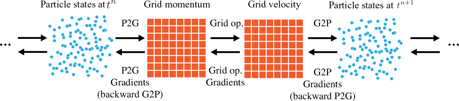
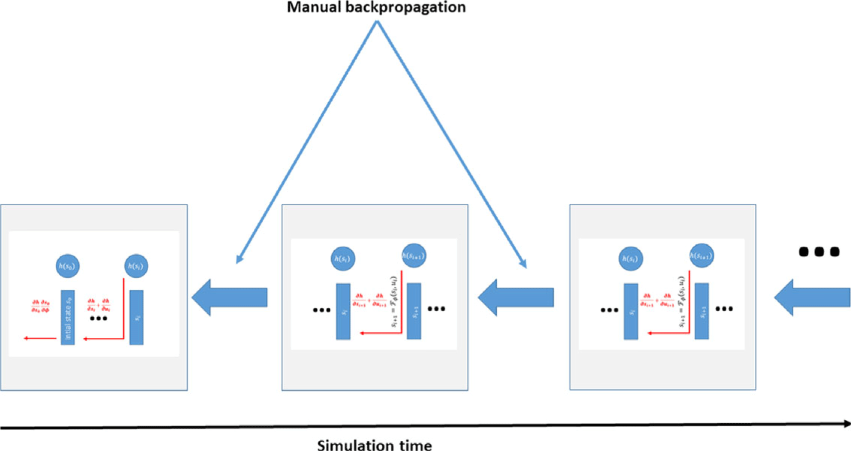
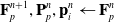
ChainQueen has two features: forward simulation, in which a soft-body simulation is timestepped forward in time, and backward propagation, in which gradients of some loss function are computed with respect to physical and controller parameters of the robot. Unlike passive soft body simulators, ChainQueen is a soft robot simulator, meaning that control signals and actuation are applied at appropriate times during the simulation. A simulation occurs over a user-specified T timesteps. The backward gradient computation procedure involves the same forward simulation operations carried out in MPM, but in a reverse order; a visual depiction can be seen in Fig. 1.
One timestep of MLS-MPM. Top arrows are for forward simulation and bottom ones are for backpropagation. A controller is embedded in the P2G process to generate actuation given particle configurations
The backpropagation graph for a timestep (which may include a final state and/or a final loss). The forward simulated system is reverse-mode autodifferentiated in order to compute gradients with respect to state, actuation, and/or controller and design parameters. A memo containing all of the relevant information for analysis is computed and maintained according to the checkpointing strategy discussed in Section 3.6
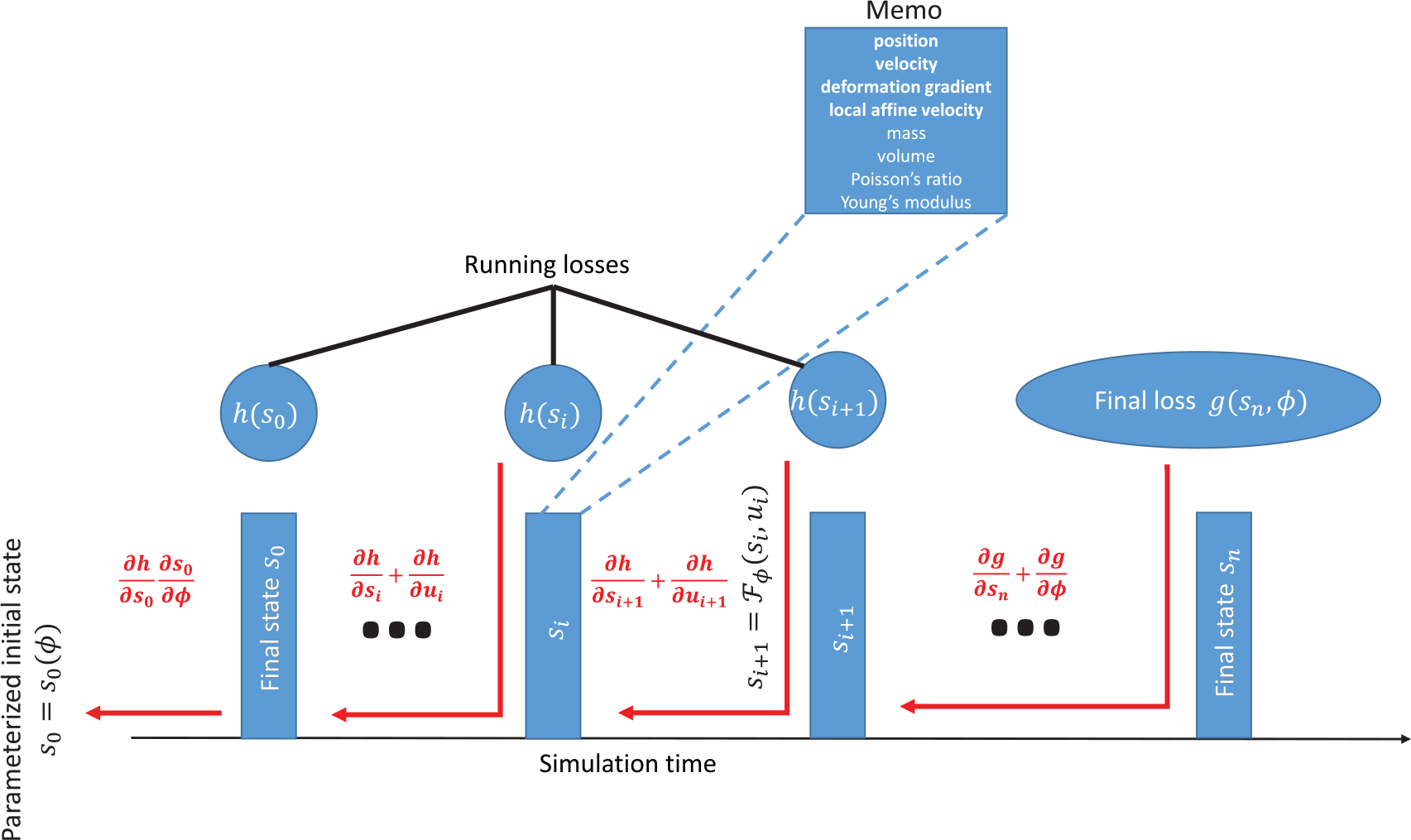
The loss function is a function which takes in a measure of the robot state (positions, velocities, deformation gradients, etc.) and actuation signal at each timestep i and a measurement of the robot’s performance. For convenience, we also define an explicit final loss for the design and the final state T. ChainQueen thus is well-suited for computing gradients with respect to loss functions of the form:
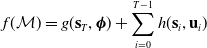 \begin{align} f(\mathcal{M}) = g(\mathbf{s}_{T}, \boldsymbol\phi) + \sum_{i=0}^{T-1} h(\mathbf{s}_{i}, \mathbf{u}_{i}) \end{align}
Here,
 $\mathcal{M}$
is referred to as the “Memo,” a descriptor of the robot state evolution throughout simulation,
$\mathcal{M}$
is referred to as the “Memo,” a descriptor of the robot state evolution throughout simulation,
 $s_i$
is the state of the robot at timestep i,
$s_i$
is the state of the robot at timestep i,
 $\mathbf{u}_i$
is the received actuation signal at timestep i, and
$\mathbf{u}_i$
is the received actuation signal at timestep i, and
 $\boldsymbol\phi$
is the static design of the robot. While
$\boldsymbol\phi$
is the static design of the robot. While
 $\mathbf{u}$
is typically a compact vector, as one can imagine,
$\mathbf{u}$
is typically a compact vector, as one can imagine,
 $\mathbf{s}$
and
$\mathbf{s}$
and
 $\mathbf{u}$
can be particularly complex, having to describe a very high-dimensional system. We describe each in turn later in this section.
$\mathbf{u}$
can be particularly complex, having to describe a very high-dimensional system. We describe each in turn later in this section.
3.2. Forward simulation
ChainQueen uses the MLS-MPM [Reference Hu, Fang, Ge, Qu, Zhu, Pradhana and Jiang20] to discretize continuum mechanics, which is governed by the following two equations:
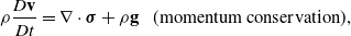 \begin{align} \rho\frac{D\mathbf{v}}{Dt} &= \nabla \cdot \boldsymbol\sigma + \rho \mathbf{g} \ \ \ \text{(momentum conservation)}, \end{align}
 \begin{align} \frac{D\rho}{Dt} + \rho \nabla \cdot \mathbf{v} &= 0 \ \ \ \text{(mass conservation)}.\end{align}
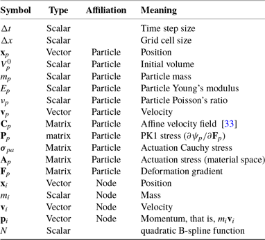
Here, we only briefly cover the basics of MLS-MPM and readers are referred to Jiang et al. [Reference Jiang, Schroeder, Teran, Stomakhin and Selle15] and Hu et al. [Reference Hu, Fang, Ge, Qu, Zhu, Pradhana and Jiang20] for a comprehensive introduction of MPM and MLS-MPM, respectively. The MPM is a hybrid Eulerian–Lagrangian method, where both particles and grid nodes are used. Simulation state information is transferred back-and-forth between these two representations. We summarize the notations we use in this paper in the table in Appendix A.I. Subscripts are used to denote particle (p) and grid nodes (i), while superscripts such as n and
 $n+1$
are used to distinguish quantities in different timesteps. The MLS-MPM simulation cycle has three steps:
$n+1$
are used to distinguish quantities in different timesteps. The MLS-MPM simulation cycle has three steps:
-
(1). Particle-to-grid transfer (P2G). Particles transfer mass
 $m_p$
, momentum
$(m\mathbf{v})_p^n$
, and stress-contributed impulse to their neighboring grid nodes, using the Affine Particle-in-Cell method [Reference Jiang, Schroeder, Selle, Teran and Stomakhin33] and MLS force discretization [Reference Hu, Fang, Ge, Qu, Zhu, Pradhana and Jiang20], weighted by a compact B-spline kernel N: (
$\mathbf{G}_p^n$
below is a temporary tensor) (4)
\begin{align}m_i^{n} & = \sum_p N(\mathbf{x}_i-\mathbf{x}_p^n)m_p,\end{align}
(5)
\begin{align}\mathbf{G}_p^n&=-\frac{4}{\Delta x^2}\Delta t V_p^0\mathbf{P}_p^n\mathbf{F}_p^{nT} + m_p \mathbf{C}_p^n,\end{align}
(6)
\begin{align}\small\mathbf{p}_i^{n} & = \sum_p N(\mathbf{x}_i- \mathbf{x}_p^n) \left[m_p\mathbf{v}_p^n+\mathbf{G}_p^n(\mathbf{x}_i-\mathbf{x}_p^n)\right].\end{align}
$m_p$
, momentum
$(m\mathbf{v})_p^n$
, and stress-contributed impulse to their neighboring grid nodes, using the Affine Particle-in-Cell method [Reference Jiang, Schroeder, Selle, Teran and Stomakhin33] and MLS force discretization [Reference Hu, Fang, Ge, Qu, Zhu, Pradhana and Jiang20], weighted by a compact B-spline kernel N: (
$\mathbf{G}_p^n$
below is a temporary tensor) (4)
\begin{align}m_i^{n} & = \sum_p N(\mathbf{x}_i-\mathbf{x}_p^n)m_p,\end{align}
(5)
\begin{align}\mathbf{G}_p^n&=-\frac{4}{\Delta x^2}\Delta t V_p^0\mathbf{P}_p^n\mathbf{F}_p^{nT} + m_p \mathbf{C}_p^n,\end{align}
(6)
\begin{align}\small\mathbf{p}_i^{n} & = \sum_p N(\mathbf{x}_i- \mathbf{x}_p^n) \left[m_p\mathbf{v}_p^n+\mathbf{G}_p^n(\mathbf{x}_i-\mathbf{x}_p^n)\right].\end{align}
-
(2). Grid operations. Grid momentum is normalized into grid velocity after division by grid mass:
(7)Note that neighboring particles interact with each other through their shared grid nodes, and collisions are handled automatically. Here, we omit boundary conditions and gravity for simplicity.
\begin{align}\mathbf{v}_i^{n} & = \frac{1}{m_i^n}\mathbf{p}_i^n.\end{align}
-
(3). Grid-to-particle transfer (G2P). Particles gather updated velocity
$\mathbf{v}_p^{n+1}$
, local velocity field gradients
$\mathbf{C}_p^{n+1}$
, and position
$\mathbf{x}_p^{n+1}$
. The constitutive model properties (e.g., deformation gradients
$\mathbf{F}_p^{n+1}$
) are updated. (8)
\begin{align}\mathbf{v}_p^{n+1} & = \sum_i N(\mathbf{x}_i- \mathbf{x}_p^n)\mathbf{v}_i^n, \end{align}
(9)
\begin{align}\mathbf{C}_p^{n+1} & = \frac{4}{\Delta x^2} \sum_i N(\mathbf{x}_i- \mathbf{x}_p^n)\mathbf{v}_i^n(\mathbf{x}_i-\mathbf{x}_p^n)^T, \end{align}
(10)
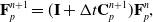
\begin{align}\mathbf{F}_p^{n+1} & = (\mathbf{I} + \Delta t \mathbf{C}_p^{n+1})\mathbf{F}_p^n, \end{align}
(11)
\begin{align}\mathbf{x}_p^{n+1} & = \mathbf{x}_p^n + \Delta t \mathbf{v}_p^{n+1}.\end{align}


Boundary conditions (Contact models)
ChainQueen adopts four commonly used MPM boundary conditions from computer graphics [Reference Stomakhin, Schroeder, Chai, Teran and Selle16]. These boundary conditions happen on the grid, after Eq. (7). Denoting the grid node velocity as
 $\mathbf{v}$
and local boundary normal as
$\mathbf{v}$
and local boundary normal as
 $\mathbf{n}$
, the four boundary conditions are
$\mathbf{n}$
, the four boundary conditions are
Sticky Directly set the grid node velocity to
 $\mathbf{0}$
. That is,
$\mathbf{0}$
. That is,
 $\mathbf{v} \leftarrow \mathbf{0}$
.
$\mathbf{v} \leftarrow \mathbf{0}$
.
Slip Set the normal component of the grid node velocity to 0. That is,
 $\mathbf{v} \leftarrow \mathbf{v} - (\mathbf{v} \cdot \mathbf{n})\mathbf{n}$
.
$\mathbf{v} \leftarrow \mathbf{v} - (\mathbf{v} \cdot \mathbf{n})\mathbf{n}$
.
Seperate If the velocity is moving away from the boundary
 $(\mathbf{v} \cdot \mathbf{n} > 0)$
then do nothing. Otherwise use Slip. This can be considered as a special case (coefficient of friction
$(\mathbf{v} \cdot \mathbf{n} > 0)$
then do nothing. Otherwise use Slip. This can be considered as a special case (coefficient of friction
 $=0$
) of Friction.
$=0$
) of Friction.
Friction If the velocity is moving away from the boundary
 $(\mathbf{v} \cdot \mathbf{n} > 0)$
, then do nothing. Otherwise apply Coulomb’s law of friction to compute the new tangential and normal components of velocity after collision and friction.
$(\mathbf{v} \cdot \mathbf{n} > 0)$
, then do nothing. Otherwise apply Coulomb’s law of friction to compute the new tangential and normal components of velocity after collision and friction.
3.3. Material models
We extend ChainQueen’s original material model, which was simply fixed corotated material, in order to further support Neohookean materials as well. We emphasize that other material models can be simply, modularly added as an option in ChainQueen, so long as they are differentiable.
The difference between Neohookean, corotated, and linear materials has been well studied and documented [Reference Bonet and Wood34–Reference Smith, De Goes and Kim36], especially in the static load case. We direct the reader to the accompanying video, for a simple example of material model choice on a nearly incompressible oscillating actuator, demonstrating a modest, but not insignificant effect that choice of material model can have on a soft robot’s dynamical response. The (wall-time) difference in the computational cost of the Neohookean and corotated models is negligible.
Fixed corotated
The fixed corotated material model [Reference Stomakhin, Howes, Schroeder and Teran37] is defined as having first Piola–Kirchhoff stress function
 $\mathbf{P}$
:
$\mathbf{P}$
:
 \begin{align}\mathbf{P}(\mathbf{F}) = 2 \mu (\mathbf{F}-\mathbf{R}) + \lambda (J-1)J \mathbf{F}^{-T}\end{align}
where
 $J = \det(\mathbf{F})$
, and
$J = \det(\mathbf{F})$
, and
 $\lambda$
and
$\lambda$
and
 $\mu$
are the first and second LamÉ parameters, determined by the material’s Young’s modulus and Poisson’s ratio. Here,
$\mu$
are the first and second LamÉ parameters, determined by the material’s Young’s modulus and Poisson’s ratio. Here,
 $\mathbf{R}$
is the rotational component of
$\mathbf{R}$
is the rotational component of
 $\mathbf{F}$
, computable via the (differentiable) polar decomposition.
$\mathbf{F}$
, computable via the (differentiable) polar decomposition.
Neohookean
The Neohookean material model is especially popular in modeling nonlinear rubbers and silicones. The Neohookean elastic stress tensor is defined as:
 \begin{align} \mathbf{P}(\mathbf{F}) = \mu(\mathbf{F} - \mathbf{F}^{-T}) + \lambda \log(J) \mathbf{F}^{-T}\end{align}
Although this energy model possesses a pole at
 $J=0$
, this corresponds to the situation where the material is compressed to a singularity. While instability caused by this singularity can happen in practice in general, it rarely occurs in the types of systems explored here, and never happened in any of our experiments. \footnote Note that in MPM the update of J (i.e.,
$J=0$
, this corresponds to the situation where the material is compressed to a singularity. While instability caused by this singularity can happen in practice in general, it rarely occurs in the types of systems explored here, and never happened in any of our experiments. \footnote Note that in MPM the update of J (i.e.,
 $\textbf{det}(F)$
) is multiplicative instead of additive; getting
$\textbf{det}(F)$
) is multiplicative instead of additive; getting
 $J \le 0$
is rare in our domain. Inversions are still a serious topic of investigation for many other applications in MPM and MPM at large.
$J \le 0$
is rare in our domain. Inversions are still a serious topic of investigation for many other applications in MPM and MPM at large.
Incompressible materials
Materials may be made approximately incompressible by adding a stress, as described by Bonet and Wood [Reference Bonet and Wood34]. In this scenario, an additional incompressibility stress tensor is added to the original stress tensor:
 $\mathbf{P} = \mathbf{P}_{elastic} + \mathbf{P}_{inc}$
:
$\mathbf{P} = \mathbf{P}_{elastic} + \mathbf{P}_{inc}$
:
 \begin{align} \mathbf{P}_{inc}(\mathbf{F}) = \frac{E}{3 (2 - 2 \nu)} p (J - 1)^{p-1} J \mathbf{F}^{-T}\end{align}
where p is a parameter
 $ \geq 2$
. The larger p is chosen, the more strongly incompressibility will be enforced. The ability to simulate incompressible materials is included in our ChainQueen extensions.
$ \geq 2$
. The larger p is chosen, the more strongly incompressibility will be enforced. The ability to simulate incompressible materials is included in our ChainQueen extensions.
3.4. Actuation models
Designed to model real-world soft robots, our extended ChainQueen implementation supports two common actuation models found in soft robots. The first, aimed at modeling fluidic actuators, is a stress-based actuation model. The second, which we present here and aimed at modeling cable-based actuation, is a force-based actuation model. These models are physically based and do not inject any net fictitious forces or pressures to the system (thus respecting Newton’s third law). We modify the classical MLS-MPM formulation with two additional steps in order to account for application of the actuation.
In order to model stress-based (including fluidic) actuators, we have designed an actuation model that stretches a given particle p with an additional Cauchy stress:
 \begin{align}\mathbf{A}_p=\mathbf{F}_p\boldsymbol\sigma_{pa}^{}\mathbf{F}_p^T\end{align}
Here,
 $\boldsymbol\sigma_{pa}=\text{diag}(a_x, a_y, a_z)$
. This equation corresponds to the stress in material space. Particles corresponding to a given actuator are assigned at robot design time; each actuator thus affects many corresponding particles applying the same stress. Note that this formulation naturally allows for both isotropic and anisotropic pressure actuators, useful for modeling directionally constrained actuators (e.g., Sun et al. [Reference Sun, Song, Liang and Ren38]). Already, this model is well-suited for modeling stress-based actuators (e.g., Hara et al. [Reference Hara, Zama, Takashima and Kaneto39]) and pneumatic actuators (e.g., Marchese et al. [Reference Marchese, Katzschmann and Rus40]). This model is similarly well-suited to simulating hydraulic actuators, modeling the actuator’s particles as incompressible, as previously described in Section 3.3.
$\boldsymbol\sigma_{pa}=\text{diag}(a_x, a_y, a_z)$
. This equation corresponds to the stress in material space. Particles corresponding to a given actuator are assigned at robot design time; each actuator thus affects many corresponding particles applying the same stress. Note that this formulation naturally allows for both isotropic and anisotropic pressure actuators, useful for modeling directionally constrained actuators (e.g., Sun et al. [Reference Sun, Song, Liang and Ren38]). Already, this model is well-suited for modeling stress-based actuators (e.g., Hara et al. [Reference Hara, Zama, Takashima and Kaneto39]) and pneumatic actuators (e.g., Marchese et al. [Reference Marchese, Katzschmann and Rus40]). This model is similarly well-suited to simulating hydraulic actuators, modeling the actuator’s particles as incompressible, as previously described in Section 3.3.
In order to model force-based actuators, such as cable-driven actuators, we simply integrate these forces when updating our particle velocity, creating an additional summable velocity term,
 $\mathbf{v}_{act}$
:
$\mathbf{v}_{act}$
:
 \begin{align} \mathbf{v}_{act} = \mathbf{f}_{act} dt { / m}\end{align}
Velocities, forces, and masses here refer to particle states. Here,
 $\mathbf{f}_{act}$
is computed as some user-defined force model. We detail one such model here, which also provides a concrete example of how actuation signals can be applied.
$\mathbf{f}_{act}$
is computed as some user-defined force model. We detail one such model here, which also provides a concrete example of how actuation signals can be applied.
Let
 $\{\mathbf{p}_i\}$
be an ordered sequence of r particles through which a cable is routed. Let the actuation signal associated with this actuator be the scalar u, and let R be the rest length of the cable. We then model a cable energy, based off Hooke’s law:
$\{\mathbf{p}_i\}$
be an ordered sequence of r particles through which a cable is routed. Let the actuation signal associated with this actuator be the scalar u, and let R be the rest length of the cable. We then model a cable energy, based off Hooke’s law:
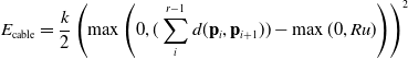 \begin{align} E_{\text{cable}} = \frac{k}{2}\left(\max{\left(0, (\sum_{i}^{r-1} d(\mathbf{p}_i, \mathbf{p}_{i+1})) - \max{(0, Ru)}\right)}\right)^2\end{align}
Here, and throughout our simulator, we assume actuation signals to be normalized between
 $-1$
and 1. d is the
$-1$
and 1. d is the
 $L_2$
distance function and k is a user-defined cable stiffness. Here, the summation computes the distance the cable must span, and Ru is the true length of the cable given the current actuation parameters (L can be thought of as a fraction of unspooled cable since we clamp it to be positive). If the true length of the cable is larger than the summed particle distance, then there is slack in the cable, and thus no stored energy. Otherwise, the cable stores an energy related to the difference in these quantities, much like a linear spring. Forces are computed by differentiating the energy with respect to positions (which can be computed easily in TensorFlow via tf.gradients with respect to the positions at timestep i) and integrated as described above.
$L_2$
distance function and k is a user-defined cable stiffness. Here, the summation computes the distance the cable must span, and Ru is the true length of the cable given the current actuation parameters (L can be thought of as a fraction of unspooled cable since we clamp it to be positive). If the true length of the cable is larger than the summed particle distance, then there is slack in the cable, and thus no stored energy. Otherwise, the cable stores an energy related to the difference in these quantities, much like a linear spring. Forces are computed by differentiating the energy with respect to positions (which can be computed easily in TensorFlow via tf.gradients with respect to the positions at timestep i) and integrated as described above.
3.5. Backpropagation
In order to compute gradients of losses of the form of Eq. (1), we apply the following backward propagation scheme. First, we assume a memo
 $\mathcal{M}$
computed via a forward simulation is available. We begin by computing gradients with respect to the final loss g, as
$\mathcal{M}$
computed via a forward simulation is available. We begin by computing gradients with respect to the final loss g, as
 $\frac{\partial l_T}{\partial \mathcal{M}} = \frac{\partial g}{\partial s_T} + \frac{\partial g}{\partial \phi}$
the partial derivative with respect to the final state, we then recursively compute:
$\frac{\partial l_T}{\partial \mathcal{M}} = \frac{\partial g}{\partial s_T} + \frac{\partial g}{\partial \phi}$
the partial derivative with respect to the final state, we then recursively compute:
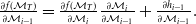 $\frac{\partial f(\mathcal{M}_T)}{\partial \mathcal{M}_{i-1}} = \frac{\partial f(\mathcal{M}_T)}{\partial \mathcal{M}_{i}} \frac{\partial \mathcal{M}_{i}}{\partial \mathcal{M}_{i-1}} + \frac{\partial h_{i-1}}{\partial \mathcal{M}_{i-1}}.$
Computing
 $\frac{\partial \mathcal{M}_i}{\partial \mathcal{M}_{i-1}}$
is highly nontrivial and, in the absence of an autodifferentiation framework, requires extensive manual derivation. While one can implement an autodifferentiated version (in TensorFlow), implementation’s enormous graph is far too slow (both in compilation and runtime) to be practical for complex tasks. To remedy this, we manually derived the simulation gradients
$\frac{\partial \mathcal{M}_i}{\partial \mathcal{M}_{i-1}}$
is highly nontrivial and, in the absence of an autodifferentiation framework, requires extensive manual derivation. While one can implement an autodifferentiated version (in TensorFlow), implementation’s enormous graph is far too slow (both in compilation and runtime) to be practical for complex tasks. To remedy this, we manually derived the simulation gradients
 $\frac{\partial \mathcal{M}_i}{\partial \mathcal{M}_{i-1}}$
and packaged them along with forward simulation in highly optimized GPU kernels. For the full details of the backward propagation derivation, please see Appendix A.2.
$\frac{\partial \mathcal{M}_i}{\partial \mathcal{M}_{i-1}}$
and packaged them along with forward simulation in highly optimized GPU kernels. For the full details of the backward propagation derivation, please see Appendix A.2.
3.6. Practical implementation
Although we have provided all the ingredients for our fully differentiable MPM simulation, we describe two optimizations which make practical implementation fast and efficient.
First, it may be tempting to create a TensorFlow graph which adds each instance of our simulation kernel (along with any control code) to one large graph, and backpropagate through the entire graph with a single call to tf.gradients. Unfortunately, we have found the TensorFlow’s compiler is unable to efficiently optimize such a graph (despite its simplicity). Therefore, we build a graph that simply includes a single simulation step (with control) and manually perform backpropagation by iteratively calling tf.gradients. That graph, whose construction we describe in more detail in Section 4, can be seen in Fig. 3.
Each step is, in itself, a large TensorFlow graph (from Fig. 2), which the TensorFlow compiler is ill-suited to optimize. For practical efficiency, we compute only the gradients with respect to individual timesteps, and manually backpropagate them using tf.gradients
Second, although a scene may need to be simulated at a small dt for physical stability, real-world controllers typically run at a much lower frequency. In order to account for this, we allow for substepping, in which the simulation kernel is executed many times at a smaller timestep between simulation steps for stability. The number of substeps, b, to use is a user parameter that can be chosen, and the effective timestep used in that kernel is set to
 $\frac{dt}{b}$
. Since TensorFlow-native controllers are typically orders of magnitude slower to execute than our MPM kernel, substepping has the added bonus of providing faster simulation and backpropagation. This is a new optimization included in our ChainQueen extension which has two benefits. First, it greatly accelerates robot optimizations, since everything aside from the (highly optimized) timestepping kernel is the bottleneck. Second, it allows us to more faithfully model real-world robots, which might have limited controller frequencies.
$\frac{dt}{b}$
. Since TensorFlow-native controllers are typically orders of magnitude slower to execute than our MPM kernel, substepping has the added bonus of providing faster simulation and backpropagation. This is a new optimization included in our ChainQueen extension which has two benefits. First, it greatly accelerates robot optimizations, since everything aside from the (highly optimized) timestepping kernel is the bottleneck. Second, it allows us to more faithfully model real-world robots, which might have limited controller frequencies.
The memory consumption to store all simulation steps is proportional to the number of timesteps. In practice when the number of timesteps N is high, the memory consumption may grow as O(N). In order to reduce memory consumption, we apply a checkpointing trick here to trade time for space. We partition the whole simulation into
 $O(\sqrt{N})$
segments, each with
$O(\sqrt{N})$
segments, each with
 $O(\sqrt{N})$
timesteps. During forward simulation, we memorize not only the latest simulation state but also the initial simulation state of each segment. This means we only have to memorize
$O(\sqrt{N})$
timesteps. During forward simulation, we memorize not only the latest simulation state but also the initial simulation state of each segment. This means we only have to memorize
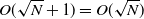 $O(\sqrt{N} + 1) = O(\sqrt{N})$
states. During backpropagation, we compute the gradients in a segment-wise manner, from the final segment to the initial segment. For each segment, we first recompute all the timesteps and store the results. This would result in
$O(\sqrt{N} + 1) = O(\sqrt{N})$
states. During backpropagation, we compute the gradients in a segment-wise manner, from the final segment to the initial segment. For each segment, we first recompute all the timesteps and store the results. This would result in
 $O(\sqrt{N})$
temporary simulation states. Then we can backpropagate within this segment. The total memory consumption of this checkpointing scheme is
$O(\sqrt{N})$
temporary simulation states. Then we can backpropagate within this segment. The total memory consumption of this checkpointing scheme is
 $O(\sqrt{N} + \sqrt{N}) = O(\sqrt{N})$
, which is a significant improvement over O(N). At the same time, the number of forward timesteps is
$O(\sqrt{N} + \sqrt{N}) = O(\sqrt{N})$
, which is a significant improvement over O(N). At the same time, the number of forward timesteps is
 $O(2N)=O(N)$
, and the number of backward timesteps stays O(N).
$O(2N)=O(N)$
, and the number of backward timesteps stays O(N).
3.7. Pitfalls and resilience
Despite our simulator’s strengths, there are two common failure modes which can cause soft simulation to fail. We describe each in turn, below.
Our simulator uses explicit forward Euler timestepping, meaning that the timesteps taken for each substep must be small in order to ensure stable simulation. In particular, as shown in Fang et al. [Reference Fang and Hu41], the
 $\Delta t$
limit for explicit time integration is approximately
$\Delta t$
limit for explicit time integration is approximately
 $ C \Delta x \sqrt{\frac{\rho}{E}}$
, where C is a constant close to one,
$ C \Delta x \sqrt{\frac{\rho}{E}}$
, where C is a constant close to one,
 $\rho$
is the density, and E is the Young’s modulus. This is related to the speed of sound, or the speed of vibrations as it travels through an elastic medium. In our workflow, users specify the timestep size, but must take care; if the timestep is chosen to be significantly larger than this limit, numerical explosions can occur.
$\rho$
is the density, and E is the Young’s modulus. This is related to the speed of sound, or the speed of vibrations as it travels through an elastic medium. In our workflow, users specify the timestep size, but must take care; if the timestep is chosen to be significantly larger than this limit, numerical explosions can occur.
Numerical fracture
A more subtle failure mode, but one that is present as a drawback of MPM is numerical fracture or “tearing” of the elastic medium. However, even just a few particles per cell can show resilience to numerical fracture. Please see the accompanying video for an experiment showing fast convergence in stability, even in the presence of actuation.
4. Soft robotics API
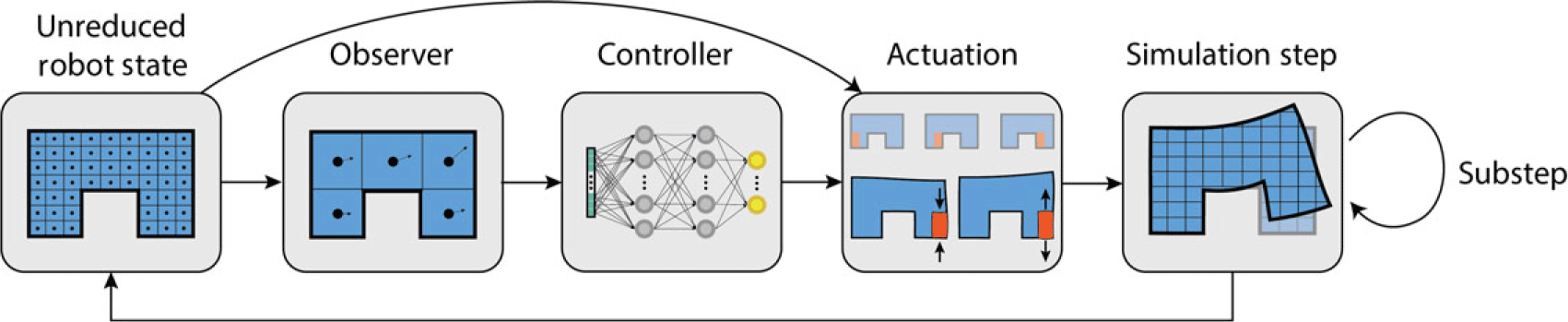
In order to streamline the design and optimization of soft robots, we have developed a simple-to-use, high-level API for interfacing with the ChainQueen physics engine. Our API abstracts the robot simulation process into four parts: observation, control, actuation, and physical timestepping. To optimize a robot for a task, users must specify an initial robot morphology (shape and materials), place actuators on the robot, choose an “observer” model, choose a controller, and specify an objective of the form in Eq. (1). Users may also select from an array of constrained and unconstrained optimizers with which to optimize the robot. Using this API, a robot co-design problem may be specified in a relatively short script. Users only need to specify the above seven items (topology, materials, actuators, observer, controller, objective, optimizer), making the conceptual workflow simple and amenable to rapid prototyping and experimentation.
In the remainder of this section, we describe in more detail how these components combine to form the TensorFlow computational graph, describe the components currently available in the API, and finally present a simple, example program to demonstrate the simplicity of our API.
Construction
Previously, we have referred to two parts of our simulation – physical simulation and control. In truth, what we describe as “control” actually is composed of multiple subcomponents. We describe these here.
Assume a robot is at a state
 $\mathbf{s}_i$
. First, that state
$\mathbf{s}_i$
. First, that state
 $\mathbf{s}_i$
is fed into what is referred to as an observer, which transforms the (very) large state description and summarizes it in what is typically a more compact form, the observation
$\mathbf{s}_i$
is fed into what is referred to as an observer, which transforms the (very) large state description and summarizes it in what is typically a more compact form, the observation
 $\mathbf{o}_i$
. This observation
$\mathbf{o}_i$
. This observation
 $\mathbf{o}_i$
is then fed into a controller in order to produce an actuation signal,
$\mathbf{o}_i$
is then fed into a controller in order to produce an actuation signal,
 $\mathbf{u}_i$
. The actuation signal is fed into the actuators in order to produce appropriate stress or forces to apply. These stresses and forces are then fed into the physical simulator, along with the state
$\mathbf{u}_i$
. The actuation signal is fed into the actuators in order to produce appropriate stress or forces to apply. These stresses and forces are then fed into the physical simulator, along with the state
 $s_i$
, and substepped b times, producing state
$s_i$
, and substepped b times, producing state
 $\mathbf{s}_{i+1}$
. At this point, we can apply the final loss g or the running loss h, depending on if
$\mathbf{s}_{i+1}$
. At this point, we can apply the final loss g or the running loss h, depending on if
 $i=T$
or not, and accumulate it into our total loss.
$i=T$
or not, and accumulate it into our total loss.
We make one final note about this accumulation process. Although as described above, the backpropagation scheme accumulates running losses through a summation, our system is easily modifiable such that other differentiable accumulation functions may be used, including
 $\max$
,
$\max$
,
 $\min$
, product, and so on. Derivation of the backpropagation scheme is mechanically similar for each of these.
$\min$
, product, and so on. Derivation of the backpropagation scheme is mechanically similar for each of these.
The entire process is demonstrated in Fig. 4.
One full step of simulation. The full state of the robot (masses, positions, and velocities of particles and grids, particle material properties, and particle volumes deformation gradients) is fed into an observer. The observer transmits a more compact summary of the full state to the controller function, which produces an output actuation. The system is then substepped a number of user-specified times with the computed actuation, resulting in the robot state for the next timestep
Choosing the objective function
Choosing the objective function amounts to choosing a final cost g, a running cost h, and an accumulator function (which we have chosen to be summation). Examples of final costs may be (the negation of) how far forward a robot has traveled, measured by the average position of its particles, or for design problems, a regularizer to keep design parameters close to their initial values. Examples of running costs include an actuation penalty (say,
 $\frac{1}{2}\mathbf{u}_i^T\mathbf{u}_i$
), which is popular for keeping robots energy efficient. Objectives may be weighted in order to trade off their relative importance.
$\frac{1}{2}\mathbf{u}_i^T\mathbf{u}_i$
), which is popular for keeping robots energy efficient. Objectives may be weighted in order to trade off their relative importance.
Observers
As described, observers translate potentially high dimensional states into typically low dimensional observations. Our API currently supports two observation models. In the first observation model, the centroid observer computes the center of position, velocity, and/or acceleration of manually, or automatically segmented particle clusters, and concatenates these vectors into a long observation vector. The second observation model (also known as the convolutional variational autoencoder, observer) applies a convolutional encoder to the grid cells and returns the latent space as the observer. The autoencoder may be trained offline or in-the-loop (as in Spielberg et al. [Reference Spielberg, Zhao, Hu, Du, Matusik and Rus42]). We expose the API as described in Listing A.1 in order to allow users to easily define their own custom observation functions.
Controllers
Controllers translate (typically compact) observations into actuation signal. Our API currently supports two controller models. The first is an open-loop controller, which simply maintains an actuation vector for each timestep and returns it (notice this controller does not consume the observation in any way). The second, a closed-loop neural network controller, applies a multi-layer perceptron and returns an actuation output. The API for users to extend is described in Listing A.1.
Actuators
Actuators translate actuation signals into stresses or forces to be applied in simulation. An example of each is described in Section 3.4. The API for users to extend is presented in Fig. A.1.
Optimizers
We have created wrappers for PyGMO [43] and TensorFlow’s internal first-order optimizers in order to allow users to easily experiment with both first-order and second-order optimizers. Our first-order optimizer wrapper also allows for variable bounds (maintained via a projection operator, in order to keep physical design parameters within reasonable bounds). Our second-order optimizer allows users to solve problems with complex equality and inequality constraints. Further optimizers could include, for example, the Learning-In-The-Loop optimizer from Spielberg et al. [Reference Spielberg, Zhao, Hu, Du, Matusik and Rus42]. Users are free to define their own optimizers; the API is described in Listing 9.
Other utilities
In addition to the aforementioned components, a library of useful functions is also provided to the user. These include the ability to load robot geometries directly from image files and meshes, in order to simplify the topological design of the robot.
5. Applications
We demonstrate our enhancements to ChainQueen on three classes of applications: inference tasks, in which we algorithmically reason about the physical properties of a simulated system; pure control tasks, in which we optimize control parameters for some target robot performance, and co-optimization tasks, in which we simultaneously co-optimize robot control and design. All units used in the following experiments are in a dimensionless system; for scale, robot models are on the order of around 0.3–0.5 in max length. Please see the accompanying video for simulations and optimized designs. For even more experiments, including experiments which demonstrate dominance over model-free approaches such as reinforcement learning, please see the original ChainQueen manuscript [Reference Hu, Liu, Spielberg, Tenenbaum, Freeman, Wu, Rus and Matusik1].
For all experiments, the more physically realistic Neohookean materials were chosen, as fixed co-rotated materials were showcased in the original ChainQueen paper.
All experiments were performed on a laptop with a 2.9GHz i7 Intel processor, NVIDIA GeForce GTX 1080 graphics card, and 32GB of RAM.
In all drawings of robots at rest in the following sections, visible pneumatic actuators have been segmented with black lines and labeled with red circles.
5.1. Inference
We demonstrate the ability of ChainQueen to determine the physical parameters of simulated objects. Given a sequence of keyframes to match or a final pose to match, we define l, which corresponds to the running loss h or the final loss g as:
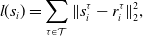 \begin{align} l(s_i) = \sum_\mathcal{\tau \in T} \|s_i^{\tau} - r_i^{\tau}\|_2^2,\end{align}
where r is some target reference pose at that point in time. The summation
 $\tau$
is over different trajectories in a set
$\tau$
is over different trajectories in a set
 $\mathcal{T}$
, generated by different fixed, specified actuation sequences, allowing users to fit robustly to multiple data sequences.
$\mathcal{T}$
, generated by different fixed, specified actuation sequences, allowing users to fit robustly to multiple data sequences.
We minimize this loss using first-order optimization, using the Adam [Reference Kingma and Ba44] optimizer. In the case where one optimizes over multiple trajectories, stochastic gradient descent is performed over the set of given trajectories.
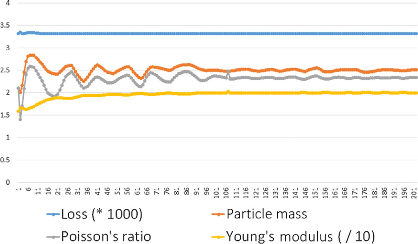
In our demonstration, we attempt to fit three homogeneous material parameters – Young’s modulus, Poisson’s ratio, and density (as specified by particle mass) – to reconstruct the trajectory of a dynamically bending, 2D, cable-driven soft finger. The finger has two cables, one on the left side and one on the right side, and is pulled in 10 different leftward-bending trajectories (generated from 10 different actuation sequences). Keyframes (200) are recorded from each trajectory. Ten copies of each trajectory are created, with noise added normally to each of 100 tracked particles (used for measuring trajectory fitting accuracy). This is used in lieu of the ground-truth trajectory, in order to emulate motion capture error. Ground truth for trajectory generation was set to 20 for Young’s Modulus, 2.33 for particle mass, and 0.25 for the Poisson’s ratio. Please see the video for animations of the simulations we fit to. Before optimizing, initial guesses were set to 15 for Young’s Modulus, 3.0 for particle mass, and 0.3 for the Poisson’s ratio. The loss was chosen to be the average squared particle distance of 100 chosen particles on the soft arm over all trajectories; this was optimized using stochastic gradient descent over the dataset of trajectories. Results can be seen in Fig. 5, featuring convergence of loss and the three constitutive material parameters. (The loss and Young’s Modulus were rescaled in this plot in order to put all plots on the same plot.)
Convergence of system identification for the soft finger. All material parameters converge to their initial values within around 100 epochs of SGD. The x-axis presents epochs of SGD, while the y-axis meaning depends on the trend-line observed. While the loss does not appear to change much in the absolute scale, this is a local (and ground truth) minimum. It cannot converge completely to 0 due to the noise added to the dataset
5.2. Control
We begin our control experiments by demonstrating a few pure control tasks. These include a 2D cable-driven Biped, a 2D Rhino loaded from a.png file, a 2D pneumatically powered biped on graded terrain, and a pneumatically powered “Bulbasaur” (modeled after the PokÉmon) loaded directly from a.stl file. We describe each briefly here; specifics of the parameters of each experiment can be found in Appendix D. The cable-driven 2D walker is an open-loop control example, the others are all closed-loop control using a MLP (2 hidden layers of 64 neurons) controller. All examples in this section were optimized via the Adam optimizer. For all tasks demonstrated here, the objective is for the robot to walk forward as far as possible in the allotted time, thus
 $g(\mathbf{s}_T) = -\mathbf{x}_T$
, where
$g(\mathbf{s}_T) = -\mathbf{x}_T$
, where
 $\mathbf{x}_T$
is the mean of the robot’s particles, A small actuation regularizer
$\mathbf{x}_T$
is the mean of the robot’s particles, A small actuation regularizer
 $h(\mathbf{u_i}) = \frac{10^{-6}}{2}\mathbf{u}_i^T\mathbf{u}_i$
was added as a running cost to each experiment to regularize the motion. Each experiment in this section was repeated 10 times; 90% confidence intervals are presented for each experiment.
$h(\mathbf{u_i}) = \frac{10^{-6}}{2}\mathbf{u}_i^T\mathbf{u}_i$
was added as a running cost to each experiment to regularize the motion. Each experiment in this section was repeated 10 times; 90% confidence intervals are presented for each experiment.
Please see the accompanying video for demonstrations of the optimized controllers.
2D cable-driven walker
In this example, we demonstrate a first, simple 2D locomotion example. A 2D biped with a cable running down each of its legs is tasked with walking forward. These cables are able to contract from their rest pose (but not expand). They are offset from the center; contracting a cable causes the leg to bend toward that cable, allowing the robot to walk. This problem has 5024 particles, for 10,048 DoFs. In this example, the goal is for the robot to walk as far forward (to the right) as possible in the allotted time. Figure 6 presents a rendering of the biped and the progress of the biped with optimization iteration and wall time, demonstrating that this problem can make significant progress (walking two body lengths) within just 5 min.
Progress of the 2D cable-driven biped versus iteration and wall-time. By pulling in an alternating motion on each of the two cables, the biped can ambulate forward
2D rhino
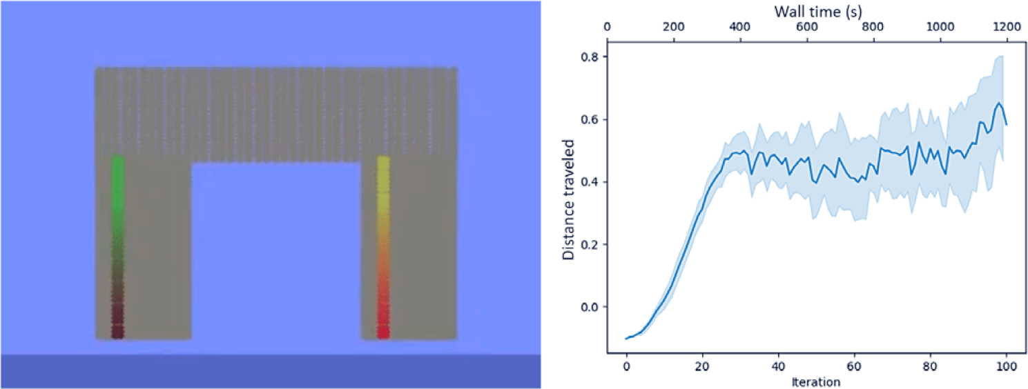
This example similarly demonstrates a simple 2D locomotion example and presents our first example of a pneumatically actuated robot. The rhino has four pneumatic actuators, two, side-by-side in each foot. Unlike the cable-driven biped, the rhino geometry and actuator placement was not instantiated manually, but rather, directly from a png image of a rhino, meaning it can be instantiated in a single line of code. Similar to the biped, however, the rhino must walk as far to the right as possible in the allotted time. The large-headed top-heavy design of the rhino makes this a dynamically challenging control task. Figure 7 presents the progress of the rhino optimization per iteration. This problem has 20,000 particles, for 40,000 DoFs.
Progress of the 2D rhino versus iteration and wall-time
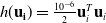
In this example, we demonstrate the ability of ChainQueen to simulate and optimize over varying terrain. In this demonstration, a 2D biped must walk as far to the right as possible in the allotted time. This task is tricky for a few reasons. First, gradients must accurately capture the effects of inter-particle collisions. Second, the optimizer must learn a control scheme that is dependent on the robot’s location in space. Third, the task itself is dynamically challenging, at times requiring the robot to be able to run up slopes of nontrivial steepness. ChainQueen is capable of all of this, and efficiently optimizes the controller for this soft robot, see Fig. 8 for details. This problem has 36,200 particles (including the terrain), for 72,400 DoFs.
Progress of the 2D biped along terrain versus iteration and wall-time
3D Bulbasaur
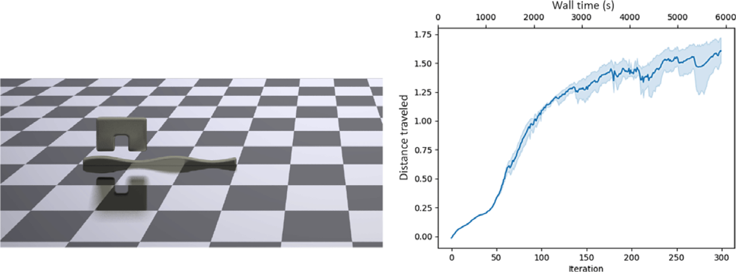
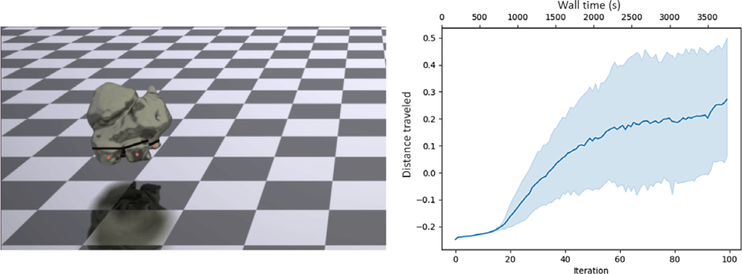
Here, we present our first 3D control optimization example, in which the robot must run as far to the right as possible in the allotted time. The Bulbasaur is instantiated directly from a.stl mesh file based off the popular video game character (with actuators then specified manually). The actuators are placed in the four quadrants of the bottom quarter of the design, which roughly places one actuator in each leg. Because of the curvature of the legs, a single actuator in each is enough to enable a lopping motion forward. Progress of the Bulbasaur optimization can be seen in Fig. 9. This problem has 22,084 particles, for 66,252 DoFs.
Progress of the 3D Bulbasaur versus iteration and wall-time
5.3. Co-design
In this section, we present a suite of open-loop and closed-loop tasks, in which we simultaneously optimize over spatially varying material parameters of the robots. Each of these examples uses pneumatic actuators.
Please see the accompanying video for demonstrations of the optimized controllers and robot designs.
5.3.1. Open-loop control
In these demonstrations, we show the ability of ChainQueen to efficiently optimize over arm reaching tasks. In these tasks, the arms must reach a target goal ball region.
3D arm
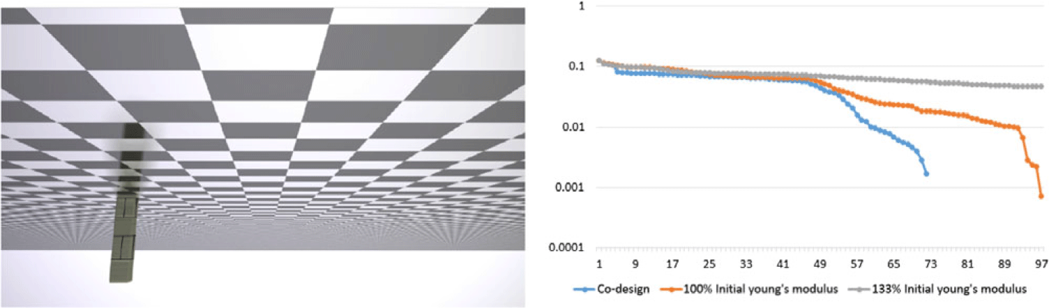
The 3D arm based on the 2D arm from the original ChainQueen manuscript is tasked with reaching a goal region with the end of its arm, shown in Fig. 10. It must further stop at this goal with 0 velocity. The arm hangs upside down from the ceiling; in this task, gravity is enabled, requiring the arm to have to “swing up” against gravity. This is a challenging task, as the stiffness of the arm and gravity requires the arm to swing back and forth in order to build up enough momentum to reach its target, like a soft analogue to a pendulum. For this experiment, we used the constrained sequential quadratic programming solver, WORHP [Reference BÜskens and Wassel45]. The experiment is performed in three configurations – with a fixed Young’s modulus = 300, at fixed Young’s modulus = 400, and with Young’s modulus initialized at 300 but co-optimized with control in a range between 150 and 400. Co-optimization dominates the fixed soft arm designs in optimization steps needed to converge to the goal. This problem has 17,280 particles, for 51,840 DoFs.
Convergence of the 3D arm reaching task for co-design versus fixed arm designs. The fixed designs take significantly longer to optimize than with co-design; it is worth noting that the final total sum-squared actuation cost of the co-optimized 3D arm is less than 75% that of the full 3D arm. Constraint violation is the norm of two constraints: distance of end-effector to goal and mean squared velocity of the particles
An example impossible without co-design
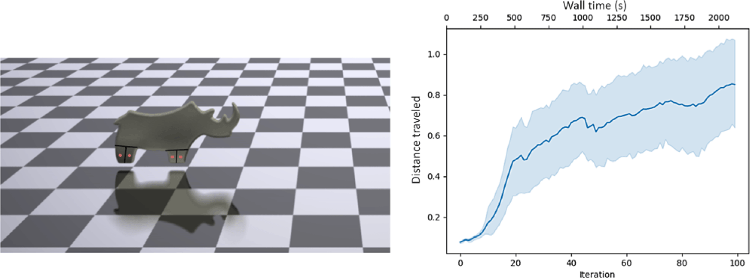
In a further open-loop control example, we present a geometrically parameterized arm, optimized via Adam. This soft arm has only a single parameter, its length, with an objective of minimizing distance of the end-effector to the goal. It must reach a target point that is too far away for it to reach in its default configuration, even with elastic stretching. In order to solve this task, the optimizer must automatically discover that the arm must lengthen to reach the goal; naturally, gradients can provide this information. This problem is successfully optimized with lower than
 $0.001$
distance error within 100 steps; please see the accompanying video for a demonstration.
$0.001$
distance error within 100 steps; please see the accompanying video for a demonstration.
This example demonstrates our system’s support for geometric parameters and shows the power of ChainQueen in enabling co-optimization tasks which transform otherwise infeasible tasks into feasible ones.
5.3.2. Closed-loop control
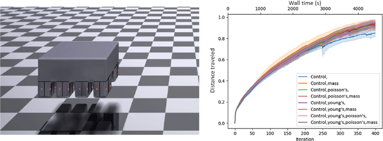
Here, we present four additional closed-loop control co-optimization tasks using an MLP (again, with two hidden layers of 64 neurons). These demonstrations – a 2D biped, a 3D quadruped, a 3D hexapod, and a 3D octoped – show ChainQueen’s ability to co-optimize over neural network controller parameters and spatially varying Young’s modulus, Poisson’s ratio, and density. In these examples, each particle has its own parameter for these three properties, meaning these problems have tens to hundreds of thousands of decision variables. Still, each of these robots can be optimized to (nearly) optimal gaits within 1 h, and often much faster. The 2D biped was run 10 times; the 3D experiments were run 6 times each.
Please see the accompanying video for full renderings of the material optimized robots. For each problem, the Young’s modulus was constrained between 7 and 20 (initial: 10), the Poisson’s ratio between 0.2 and 0.4 (initial 0.3), and the mass between 0.7 and 2.0 (initial 1.0). The maximum pressure per actuation chamber was set to 2.
2D biped
This example demonstrates a simple co-optimization example over the same biped demonstrated in the terrain example, with a goal of running as far to the right as possible in the allotted time. Every combination of the three material parameters (eight in total) was turned on and off, and run 10 times each. An interesting result, which will also follow in all 3D examples, is that each additional material parameter adds additional benefit to the co-optimization, allowing the robot to walk even farther. Furthermore, there is a clear ordering to the effect each of the material parameters has on the robot’s performance, with the Young’s modulus having the most significant impact, followed by material density, and finally Poisson’s ratio. This makes intuitive sense; the flexibility of the material will have the greatest impact in its ability to achieve optimal deformation; the density of the material then affects how easily the robots can overcome inertial forces and the effects of gravity; finally, Poisson’s ratio, while not negligible in impact, has far less of an obvious intuitive effect on soft robot locomotion. Full results can be found in Fig. 11. We highlight that optimization is extremely fast, with each biped walking several body lengths within 5 min. This problem has 12,800 particles, for 25,600 DoFs.
Progress of the 2D biped versus iteration and wall-time
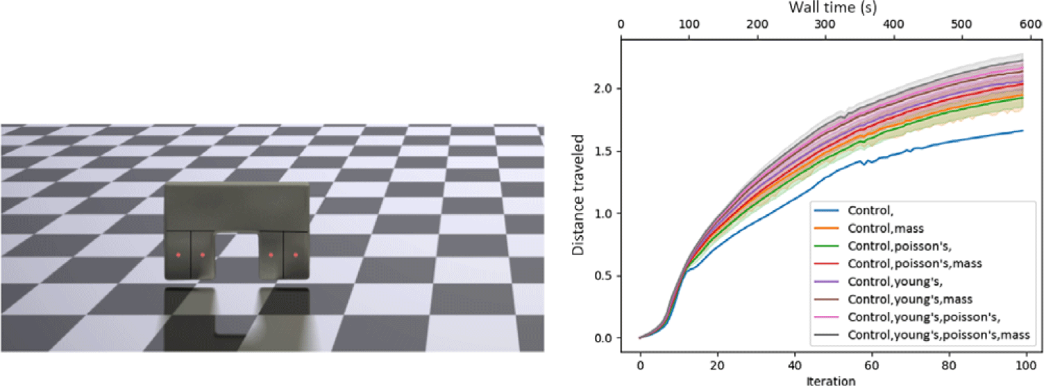
Perhaps particularly stunning is the large impact co-optimization can have on robot performance, providing a nearly 50% improvement in gait over non-co-optimized counterparts.
3D quadruped, hexapod, and octoped
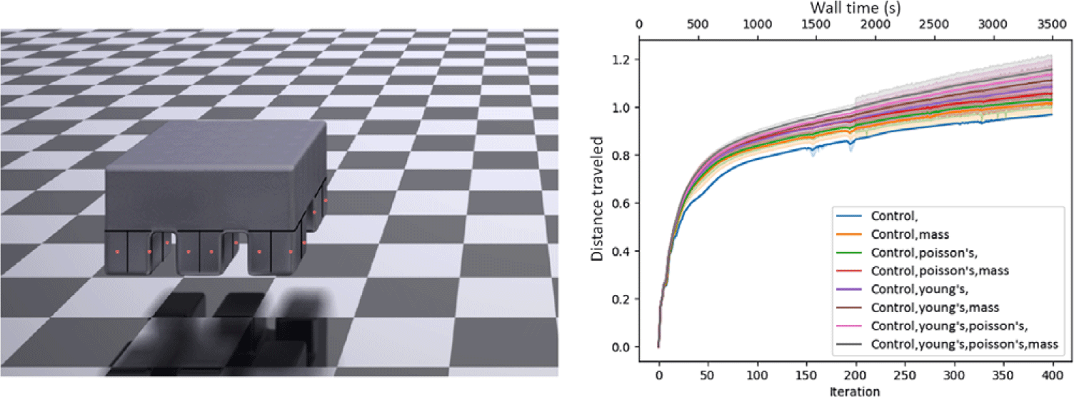
We further perform co-optimization on three complex 3D walkers, a quadruped, a hexapod, and an octoped. Each of these robots has four pressure chambers in each of its legs arranged in a square pattern. As we increase the number of legs, the robots become more dynamically complex (having more actuators) and heavier, making these tasks more challenging. Full results can be found in Figs. 12, 13, 14; these material optimization results mirror those of the 2D biped. Again, the impact of co-optimization is underscored by these graphs, as co-optimization provides a roughly 33% gain in performance for these tasks. The 3D quadruped, hexapod, and octopeds have 84,375, 111,375, and 138,375 particles for 253,125, 334,125, and 415,125 DoF, respectively.
Progress of the 3D quadruped versus iteration and wall-time

Progress of the 3D hexapod versus iteration and wall-time
Progress of the 3D octoped versus iteration and wall-time
6. Discussions and conclusions
We have documented ways we have made the ChainQueen open-source simulator more powerful, flexible, and easy to use. Further, we have highlighted the power of full spatial co-optimization of soft robots, demonstrating that they can vastly outperform their pure control-optimized counterparts in locomotion and reaching tasks. We highlight the speed of all optimization tasks presented here; thanks to our optimized GPU kernels, even large-scale problems can be solved in a matter of minutes. We are hopeful that the soft robotics community will adopt ChainQueen, along with our enhancements, as a means of accelerating soft robotics modeling for both research and industrial-grade robots.
While ChainQueen in its current state is very powerful, some challenges remain. First, more demonstrations of translations to physical robots are desired. Some simple demonstrations on actuators were presented in the original ChainQueen paper, but more sophisticated simulation to reality transfer is desired. Second, the current constitutive models do not handle viscoelastoplastic deformation; exploration of such real-world applicable materials would be an interesting direction to explore. Finally, given the efficacy of co-optimization compared to pure control optimization (as demonstrated in this paper), it would be interesting to explore fabrication methods that could realize such spatially varying programmable materials.
Acknowledgements
This work was supported by IARPA grant No. 2019-19020100001 and National Science Foundation EFRI 1830901. The authors thank Jiancheng Liu, Jiajun Wu, Joshua B. Tenenbuam, and William T. Freeman for their contributions to the original ChainQueen simulator. We thank Thingiverse user FLOWALISTIK for the Bulbasaur.stl model.
Conflicts of Interest
The author(s) declare none.
Supplementary Material
To view supplementary material for this article, please visit https://doi.org/10.1017/S0263574721000722
A. Appendix
A.1. Soft Robotics API
class Observer:
def get_dim(self):
’’’
Return the total dimension
of the observation space
as an int.
’’’
raise NotImplementedError
def observation(self, state):
’’’
Return an observation
vector of size self.get_dim(),
computed from the state.
’’’
raise NotImplementedError
def get_observation_range(self):
’’’
Return the element-wise
maximum and minimum value of the
observation space
(as a pair of vectors).
’’’
raise NotImplementedError
Listing 1:The user-defined Observer class, which converts high-dimensional robot state to a compact representation.
class Controller:
def get_controller_function(self):
’’’
Return a function that maps an
input observation (vector)
to an output actuation signal (vector).
’’’
raise NotImplementedError
Listing 2: The user-defined Controller class, which computes an actuation signal from an observation.
class Actuator:
def __init__(self, particles, is_force_actuator):
’’’The user must pass in an iterable
of ints corresponding to the sequence
of particles to be actuated.
In some cases, order may matter (cables),
in others order may not matter (fluidic actuators).
’’’
self._particles = particles
def get_actuation(self, control, state):
’’’
Given a control input signal normalized between -1 and 1
and the state of the simulation, return a
force vector (n * dim) or a pressure tensor (n * dim * dim).
(NOTE: Not all actuators need be state-dependent.)
Whether this is a force or a stress-based actuator
is inferred from the dimensionality of the output.
’’’
raise NotImplementedError
Listing 3: The user-defined Actuator class, which converts actuation signal to output force or pressure.
class Optimizer:
’’’
assume that objectives and constraints return a pair of a value
and its corresponding gradient.
Our API provides helper functions to compute these gradients.
’’’
def __init__(self, trainables, visualizer=None, **kwargs):
self._visualizer = visualize
self._trainables = trainables
self._equality_constraints = []
self._inequality_constraints = []
def setObjective(self, objective):
’’’
objective is the function to be minimized.
’’’
self._objective = objective
def addInequalityConstraint(self, constraint):
’’’
constraint is a function f interpreted in the form
f(memo) <= 0, intended to be satisfied
during optimization.
’’’
self._inequality_constraints.append(constraint)
def addEqualityConstraint(self, constraint):
’’’
constraint is a function f interpreted in the form
f(memo) = 0, intended to be satisfied
during optimization.
’’’
self._equality_constraints.append(constraint)
def optimize(self):
’’’
Optimize the objective function, subject to the constraints.
Entirely up to the user to define. Algorithms may be unconstrained
and ignore constraints at the implementer’s discretion.
’’’
raise NotImplementedError
Listing 4:The user-defined Optimizer class, which optimizes a robot given user-defined objectives and constraints.
A.2. Forward Simulation and Differentiation
In this section, we discuss the detailed steps for backward gradient computation in ChainQueen, that is, the differentiable moving least squares material point method (MLS-MPM) [Reference Hu, Fang, Ge, Qu, Zhu, Pradhana and Jiang20]. Again, we summarize the notations in Table A.1. We assume fixed particle volume
 $V_p^0$
, hyperelastic constitutive model (with potential energy
$V_p^0$
, hyperelastic constitutive model (with potential energy
 $\psi_p$
or Young’s modulus
$\psi_p$
or Young’s modulus
 $E_p$
and Poisson’s ratio
$E_p$
and Poisson’s ratio
 $\nu_p$
) for simplicity.
$\nu_p$
) for simplicity.
The list of notation for MLS-MPM is below:
A.2.1. Variable dependencies
The MLS-MPM time stepping is defined as follows:
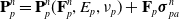 \begin{align}\mathbf{P}_p^{n} & = \mathbf{P}_p^{n}(\mathbf{F}_p^n, E_p, \nu_p)+\mathbf{F}_p\boldsymbol\sigma_{pa}^n\end{align}
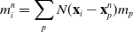 \begin{align}m_i^{n} & = \sum_p N(\mathbf{x}_i-\mathbf{x}_p^n)m_p \end{align}
 \begin{align}\mathbf{p}_i^{n} & = \sum_p N(\mathbf{x}_i- \mathbf{x}_p^n) \left[m_p\mathbf{v}_p^n+\left(-\frac{4}{\Delta x^2}\Delta t V_p^0\mathbf{P}_p^n\mathbf{F}_p^{nT} + m_p \mathbf{C}_p^n\right)(\mathbf{x}_i-\mathbf{x}_p^n)\right] \end{align}
 \begin{align}\mathbf{v}_i^{n} & = \frac{1}{m_i^n}\mathbf{p}_i^n \end{align}
 \begin{align}\mathbf{v}_p^{n+1} & = \sum_i N(\mathbf{x}_i- \mathbf{x}_p^n)\mathbf{v}_i^n \end{align}
 \begin{align}\mathbf{C}_p^{n+1} & = \frac{4}{\Delta x^2} \sum_i N(\mathbf{x}_i- \mathbf{x}_p^n)\mathbf{v}_i^n(\mathbf{x}_i-\mathbf{x}_p^n)^T \end{align}
 \begin{align}\mathbf{F}_p^{n+1} & = (\mathbf{I} + \Delta t \mathbf{C}_p^{n+1})\mathbf{F}_p^n, \end{align}
 \begin{align}\mathbf{x}_p^{n+1} & = \mathbf{x}_p^n + \Delta t \mathbf{v}_p^{n+1}\end{align}
The forward variable dependency is as follows:
 \begin{align}\mathbf{x}_p^{n+1} & \leftarrow \mathbf{x}_p^n, \mathbf{v}_p^{n+1} \end{align}
 \begin{align}\mathbf{v}_p^{n+1} & \leftarrow \mathbf{x}_p^n, \mathbf{v}_i^n \end{align}
 \begin{align}\mathbf{C}_p^{n+1} & \leftarrow \mathbf{x}_p^n, \mathbf{v}_i^n \end{align}
 \begin{align}\mathbf{F}_p^{n+1} & \leftarrow \mathbf{F}_p^n, \mathbf{C}_p^{n+1}\end{align}
 \begin{align}\mathbf{p}_i^{n} & \leftarrow \mathbf{x}_p^n, \mathbf{C}_p^n, \mathbf{v}_p^n, \mathbf{P}_p^n, \mathbf{F}_p^n, m_p^n \end{align}
 \begin{align}\mathbf{v}_i^{n} & \leftarrow \mathbf{p}_i^n, m_i^n \end{align}
 \begin{align}\mathbf{P}_p^n & \leftarrow \mathbf{F}_p^n, \boldsymbol\sigma^n_{pa}, E_p, \nu_p \end{align}
 \begin{align}m_i^{n} & \leftarrow \mathbf{x}_p^n, m_p\end{align}
During backpropagation, we have the following reversed variable dependency:
 \begin{align}\mathbf{x}_p^{n+1}, \mathbf{v}_p^{n+1}, \mathbf{C}_p^{n+1}, \mathbf{p}_i^{n+1}, m_i^{n+1} & \leftarrow \mathbf{x}_p^n \end{align}
 \begin{align}\mathbf{p}_i^{n} & \leftarrow \mathbf{v}_p^n \end{align}
 \begin{align}\mathbf{x}_p^{n+1} & \leftarrow \mathbf{v}_p^{n+1} \end{align}
 \begin{align}\mathbf{v}_p^{n+1}, \mathbf{C}_p^{n+1} & \leftarrow \mathbf{v}_i^{n} \end{align}
 \begin{align}\mathbf{F}_p^{n+1}, \mathbf{P}_p^n, \mathbf{p}_i^n & \leftarrow \mathbf{F}_p^n \end{align}
 \begin{align}\mathbf{F}_p^{n+1} & \leftarrow \mathbf{C}_p^{n+1} \end{align}
 \begin{align}\mathbf{p}_i^{n} & \leftarrow \mathbf{C}_p^n \end{align}
 \begin{align}\mathbf{v}_i^{n} & \leftarrow \mathbf{p}_i^n \end{align}
 \begin{align}\mathbf{v}_i^{n} & \leftarrow m_i^n \end{align}
 \begin{align}\mathbf{p}_i^{n} & \leftarrow \mathbf{P}_p^n \end{align}
 \begin{align}E_p & \leftarrow \mathbf{P}^n_p \end{align}
 \begin{align}\nu_p & \leftarrow \mathbf{P}^n_p \end{align}
 \begin{align}\mathbf{P}_p^n & \leftarrow \boldsymbol\sigma_{pa}^n \end{align}
 \begin{align}m_p & \leftarrow m_i^n, \mathbf{p}_i^n\end{align}
We reverse swap two sides of the equations for easier differentiation derivation:
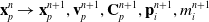 \begin{align}\mathbf{x}_p^n & \rightarrow \mathbf{x}_p^{n+1}, \mathbf{v}_p^{n+1}, \mathbf{C}_p^{n+1}, \mathbf{p}_i^{n+1}, m_i^{n+1}\end{align}
 \begin{align}\mathbf{v}_p^n & \rightarrow \mathbf{p}_p^{n}\end{align}
 \begin{align}\mathbf{v}_p^{n+1} & \rightarrow \mathbf{x}_p^{n+1}\end{align}
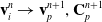 \begin{align}\mathbf{v}_i^{n} & \rightarrow \mathbf{v}_p^{n+1}, \mathbf{C}_p^{n+1}\end{align}
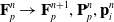 \begin{align}\mathbf{F}_p^n & \rightarrow \mathbf{F}_p^{n+1}, \mathbf{P}_p^n, \mathbf{p}_i^n \end{align}
 \begin{align}\mathbf{C}_p^{n+1} & \rightarrow \mathbf{F}_p^{n+1}\end{align}
 \begin{align}\mathbf{C}_p^n & \rightarrow \mathbf{p}_i^{n}\end{align}
 \begin{align}\mathbf{p}_i^n & \rightarrow \mathbf{v}_i^{n}\end{align}
 \begin{align}m_i^n & \rightarrow \mathbf{v}_i^{n}\end{align}
 \begin{align}\mathbf{P}_p^n & \rightarrow \mathbf{p}_i^{n}\end{align}
 \begin{align}E_p & \rightarrow \mathbf{P}^n_p \end{align}
 \begin{align}\nu_p & \rightarrow \mathbf{P}^n_p \end{align}
 \begin{align}\boldsymbol\sigma_{pa}^n & \rightarrow \mathbf{P}_p^n \end{align}
 \begin{align}m_p & \rightarrow m_i^n, \mathbf{p}_i^n\end{align}
In the following sections, we derive detailed gradient relationships, in the order of actual gradient computation. The frictional boundary condition gradients are postponed to the end since it is less central, though during computation it belongs to grid operations. Backpropagation in ChainQueen is essentially a reversed process of forward simulation. The computation has three steps, backward particle to grid (P2G), backward grid operations, and backward grid to particle (G2P).
A.2.2 Backward particle to grid (P2G)
(A, P2G) For
 $\mathbf{v}_p^{n+1}$
, we have
$\mathbf{v}_p^{n+1}$
, we have
 \begin{align}\mathbf{x}_p^{n+1} & = \mathbf{x}_p^n + \Delta t \mathbf{v}_p^{n+1}\end{align}
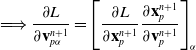 \begin{align} \Longrightarrow \frac{\partial L}{\partial {{\mathbf{v}_{p\alpha}^{n+1}}}} &= \left[\frac{\partial L}{\partial {{\mathbf{x}_p^{n+1}}}} \frac{\partial{{\mathbf{x}_p^{n+1}}}}{\partial{{\mathbf{v}_p^{n+1}}}}\right]_{\alpha} \end{align}
 \begin{align} &= \Delta t \frac{\partial L}{\partial {{\mathbf{x}_{p\alpha}^{n+1}}}}.\end{align}
(B, P2G) For
 $\mathbf{C}_p^{n+1}$
, we have
$\mathbf{C}_p^{n+1}$
, we have
 \begin{align}\mathbf{F}_p^{n+1} & = (\mathbf{I} + \Delta t \mathbf{C}_p^{n+1})\mathbf{F}_p^n \end{align}
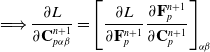 \begin{align} \Longrightarrow \frac{\partial L}{\partial {{\mathbf{C}_{p\alpha\beta}^{n+1}}}} &= \left[\frac{\partial L}{\partial {{\mathbf{F}_p^{n+1}}}} \frac{\partial{{\mathbf{F}_p^{n+1}}}}{\partial{{\mathbf{C}_p^{n+1}}}}\right]_{\alpha\beta} \end{align}
 \begin{align} &= \Delta t \sum_\gamma\frac{\partial L}{\partial {{\mathbf{F}_{p\alpha\gamma}^{n+1}}}}\mathbf{F}_{p\beta\gamma}^n.\end{align}
Note, the above two gradients should also include the contributions of
 $\frac{\partial L}{\partial {{\mathbf{v}_p^{n}}}}$
and
$\frac{\partial L}{\partial {{\mathbf{v}_p^{n}}}}$
and
 $\frac{\partial L}{\partial {{\mathbf{C}_p^{n}}}}$
, respectively, with n being the next time step.
$\frac{\partial L}{\partial {{\mathbf{C}_p^{n}}}}$
, respectively, with n being the next time step.
(C, P2G) For
 $\mathbf{v}_i^n$
, we have
$\mathbf{v}_i^n$
, we have
 \begin{align} \mathbf{v}_p^{n+1} & = \sum_i N(\mathbf{x}_i- \mathbf{x}_p^n)\mathbf{v}_i^n\end{align}
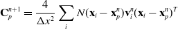 \begin{align} \mathbf{C}_p^{n+1} & = \frac{4}{\Delta x^2} \sum_i N(\mathbf{x}_i- \mathbf{x}_p^n)\mathbf{v}_i^n(\mathbf{x}_i-\mathbf{x}_p^n)^T\end{align}
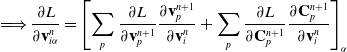 \begin{align} \Longrightarrow \frac{\partial L}{\partial {{\mathbf{v}_{i\alpha}^n}}} &= \left[\sum_p \frac{\partial L}{\partial {{\mathbf{v}_p^{n+1}}}} \frac{\partial{{\mathbf{v}_p^{n+1}}}}{\partial{{\mathbf{v}_i^n}}} + \sum_p \frac{\partial L}{\partial {{\mathbf{C}_p^{n+1}}}} \frac{\partial{{\mathbf{C}_p^{n+1}}}}{\partial{{\mathbf{v}_i^n}}}\right]_{\alpha} \end{align}
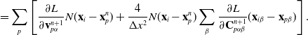 \begin{align} &= \sum_p\left[\frac{\partial L}{\partial {{\mathbf{v}_{p\alpha}^{n+1}}}}N(\mathbf{x}_i-\mathbf{x}_p^n) +\frac{4}{\Delta x^2}N(\mathbf{x}_i-\mathbf{x}_p^n)\sum_\beta \frac{\partial L}{\partial {{\mathbf{C}_{p\alpha\beta}^{n+1}}}} (\mathbf{x}_{i\beta}-\mathbf{x}_{p\beta})\right].\end{align}
A.2.3 Backward grid operations
(D, grid) For
 $\mathbf{p}_i^n$
, we have
$\mathbf{p}_i^n$
, we have
 \begin{align}\mathbf{v}_i^{n} & = \frac{1}{m_i^n}\mathbf{p}_i^n\end{align}
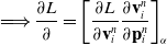 \begin{align} \Longrightarrow \frac{\partial L}{\partial {{{}}}} &= \left[\frac{\partial L}{\partial {{\mathbf{v}_i^{n}}}} \frac{\partial{{\mathbf{v}_i^{n}}}}{\partial{{\mathbf{p}_i^n}}}\right]_{\alpha}\end{align}
 \begin{align} &= \frac{\partial L}{\partial {{\mathbf{v}_{i\alpha}^{n}}}} \frac{1}{m_i^n}.\end{align}
(E, grid) For
 $m_i^n$
, we have
$m_i^n$
, we have
 \begin{align}\mathbf{v}_i^{n} & = \frac{1}{m_i^n}\mathbf{p}_i^n\end{align}
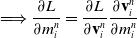 \begin{align} \Longrightarrow \frac{\partial L}{\partial {{m_{i}^n}}} &= \frac{\partial L}{\partial {{\mathbf{v}_i^{n}}}} \frac{\partial{{\mathbf{v}_i^{n}}}}{\partial{{m_i^n}}}\end{align}
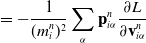 \begin{align} &= -\frac{1}{(m_i^n)^2}\sum_\alpha \mathbf{p}_{i\alpha}^{n}\frac{\partial L}{\partial {{\mathbf{v}_{i\alpha}^{n}}}} \end{align}
 \begin{align} &=-\frac{1}{m_i^n}\sum_\alpha \mathbf{v}_{i\alpha}^{n}\frac{\partial L}{\partial {{\mathbf{v}_{i\alpha}^{n}}}}.\end{align}
A.2.4 Backward grid to particle (G2P)
(F, G2P) For
 $\mathbf{v}_p^n$
, we have
$\mathbf{v}_p^n$
, we have
 \begin{align}\mathbf{p}_i^{n} & = \sum_p N(\mathbf{x}_i- \mathbf{x}_p^n) \left[m_p\mathbf{v}_p^n+\left(-\frac{4}{\Delta x^2}\Delta t V_p^0\mathbf{P}_p^n\mathbf{F}_p^{nT} + m_p \mathbf{C}_p^n\right)(\mathbf{x}_i-\mathbf{x}_p^n)\right] \end{align}
 \begin{align}\Longrightarrow \frac{\partial L}{\partial {{\mathbf{v}_{p\alpha}^n}}} &= \left[\sum_i \frac{\partial L}{\partial {{\mathbf{p}_p^{n}}}} \frac{\partial{{\mathbf{p}_p^{n}}}}{\partial{{\mathbf{v}_p^n}}}\right]_{\alpha} \end{align}
 \begin{align} &= \sum_i N(\mathbf{x}_i-\mathbf{x}_p^n) m_p \frac{\partial L}{\partial {{\mathbf{p}_{i\alpha}^n}}}.\end{align}
(G, G2P) For
 $\mathbf{P}_p^n$
, we have
$\mathbf{P}_p^n$
, we have
 \begin{align}\mathbf{p}_i^{n} & = \sum_p N(\mathbf{x}_i- \mathbf{x}_p^n) \left[m_p\mathbf{v}_p^n+\left(-\frac{4}{\Delta x^2}\Delta t V_p^0\mathbf{P}_p^n\mathbf{F}_p^{nT} + m_p \mathbf{C}_p^n\right)(\mathbf{x}_i-\mathbf{x}_p^n)\right]\end{align}
 \begin{align} \Longrightarrow \frac{\partial L}{\partial {{\mathbf{P}_{p\alpha\beta}^n}}} &= \left[\frac{\partial L}{\partial {{\mathbf{p}_i^{n}}}} \frac{\partial{{\mathbf{p}_i^{n}}}}{\partial{{\mathbf{P}_p^n}}}\right]_{\alpha\beta}\end{align}
 \begin{align} &= -\sum_iN(\mathbf{x}_i-\mathbf{x}_p^n) \frac{4}{\Delta x^2}\Delta t V_p^0 \sum_\gamma \frac{\partial L}{\partial {{\mathbf{p}_{i\alpha}^n}}} \mathbf{F}_{p_\gamma\beta}^{n}(\mathbf{x}_{i\gamma}-\mathbf{x}_{p\gamma}^n).\end{align}
(H, G2P) For
 $\mathbf{F}_p^{n}$
, we have
$\mathbf{F}_p^{n}$
, we have
 \begin{align}\mathbf{F}_p^{n+1} & = (\mathbf{I} + \Delta t \mathbf{C}_p^{n+1})\mathbf{F}_p^n \end{align}
 \begin{align}\mathbf{P}_p^{n} & = \mathbf{P}_p^{n}(\mathbf{F}_p^n, E_p, \nu_p)+\mathbf{F}_p\boldsymbol\sigma_{pa}^n \end{align}
 \begin{align}\mathbf{p}_i^{n} & = \sum_p N(\mathbf{x}_i- \mathbf{x}_p^n) \left[m_p\mathbf{v}_p^n+\left(-\frac{4}{\Delta x^2}\Delta t V_p^0\mathbf{P}_p^n\mathbf{F}_p^{nT} + m_p \mathbf{C}_p^n\right)(\mathbf{x}_i-\mathbf{x}_p^n)\right] \end{align}
 \begin{align} \Longrightarrow \frac{\partial L}{\partial {{\mathbf{F}_{p\alpha\beta}^n}}} &= \left[\frac{\partial L}{\partial {{\mathbf{F}_p^{n+1}}}} \frac{\partial{{\mathbf{F}_p^{n+1}}}}{\partial{{\mathbf{F}_p^n}}} + \frac{\partial L}{\partial {{\mathbf{P}_p^n}}} \frac{\partial{{\mathbf{P}_p^n}}}{\partial{{\mathbf{F}_p^n}}}+\frac{\partial L}{\partial {{\mathbf{p}_i^n}}} \frac{\partial{{\mathbf{p}_i^n}}}{\partial{{\mathbf{F}_p^n}}}\right]_{\alpha\beta} \end{align}
 \begin{align} &= \sum_\gamma\frac{\partial L}{\partial {{\mathbf{F}_{p\gamma\beta}^{n+1}}}}(\mathbf{I}_{\gamma\alpha}+\Delta t \mathbf{C}_{p\gamma\alpha}^{n+1}) + \sum_\gamma \sum_\eta \frac{\partial L}{\partial {{\mathbf{P}_{p\gamma\eta}}}} \frac{\partial ^2\Psi_p}{\partial \mathbf{F}^n_{p\gamma\eta} \partial \mathbf{F}_{p\alpha\beta}^n}+\sum_\gamma\frac{\partial L}{\partial {{\mathbf{P}_{p\alpha\gamma}^{n}}}}\boldsymbol\sigma_{pa\beta\gamma}\end{align}
 \begin{align} &\quad +\sum_i -N(\mathbf{x}_i-\mathbf{x}_p^n) \sum_\gamma \frac{\partial L}{\partial {{\mathbf{p}_{i\gamma}^n}}} \frac{4}{\Delta x^2} \Delta{}t V_p^0\mathbf{P}_{p\gamma\beta}^n (\mathbf{x}_{i\alpha} - \mathbf{x}_{p\alpha}^n).\end{align}
(I, G2P) For
 $\mathbf{C}_p^n$
, we have
$\mathbf{C}_p^n$
, we have
 \begin{align}\mathbf{p}_i^{n} & = \sum_p N(\mathbf{x}_i- \mathbf{x}_p^n) \left[m_p\mathbf{v}_p^n+\left(-\frac{4}{\Delta x^2}\Delta t V_p^0\mathbf{P}_p^n\mathbf{F}_p^{nT} + m_p \mathbf{C}_p^n\right)(\mathbf{x}_i-\mathbf{x}_p^n)\right]\end{align}
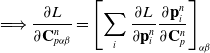 \begin{align} \Longrightarrow \frac{\partial L}{\partial {{\mathbf{C}_{p\alpha\beta}^n}}} &= \left[\sum_i\frac{\partial L}{\partial {{\mathbf{p}_i^{n}}}} \frac{\partial{{\mathbf{p}_i^{n}}}}{\partial{{\mathbf{C}_p^n}}}\right]_{\alpha\beta}\end{align}
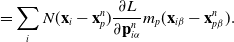 \begin{align} &= \sum_i N(\mathbf{x}_i-\mathbf{x}_p^n) \frac{\partial L}{\partial {{\mathbf{p}_{i\alpha}^{n}}}} m_p (\mathbf{x}_{i\beta}-\mathbf{x}_{p\beta}^n).\end{align}
(J, G2P) For
 $\mathbf{x}_p^n$
, we have
$\mathbf{x}_p^n$
, we have
 \begin{align} \mathbf{x}_p^{n+1} & = \mathbf{x}_p^n + \Delta t \mathbf{v}_p^{n+1} \end{align}
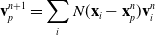 \begin{align} \mathbf{v}_p^{n+1} & = \sum_i N(\mathbf{x}_i- \mathbf{x}_p^n)\mathbf{v}_i^n \end{align}
 \begin{align} \mathbf{C}_p^{n+1} & = \frac{4}{\Delta x^2} \sum_i N(\mathbf{x}_i- \mathbf{x}_p^n)\mathbf{v}_i^n(\mathbf{x}_i-\mathbf{x}_p^n)^T \end{align}
 \begin{align} \mathbf{p}_i^{n} & = \sum_p N(\mathbf{x}_i- \mathbf{x}_p^n) \left[m_p\mathbf{v}_p^n+\left(-\frac{4}{\Delta x^2}\Delta t V_p^0\mathbf{P}_p^n\mathbf{F}_p^{nT} + m_p \mathbf{C}_p^n\right)(\mathbf{x}_i-\mathbf{x}_p^n)\right]\end{align}
 \begin{align} m_i^{n} & = \sum_p N(\mathbf{x}_i-\mathbf{x}_p^n)m_p\end{align}
 \begin{align} \mathbf{G}_p & : = \left(-\frac{4}{\Delta x^2} V_p^0\Delta{}t\mathbf{P}_p^n\mathbf{F}_p^{nT} + m_p \mathbf{C}_p^n\right)\end{align}
 \begin{align} \Longrightarrow&\end{align}
 \begin{align} \frac{\partial L}{\partial {{\mathbf{x}_{p\alpha}^{n}}}} &= \left[\frac{\partial L}{\partial {{\mathbf{x}_p^{n+1}}}} \frac{\partial{{\mathbf{x}_p^{n+1}}}}{\partial{{\mathbf{x}_p^n}}} +\frac{\partial L}{\partial {{\mathbf{v}_p^{n+1}}}} \frac{\partial{{\mathbf{v}_p^{n+1}}}}{\partial{{\mathbf{x}_p^n}}} +\frac{\partial L}{\partial {{\mathbf{C}_p^{n+1}}}} \frac{\partial{{\mathbf{C}_p^{n+1}}}}{\partial{{\mathbf{x}_p^n}}} +\frac{\partial L}{\partial {{\mathbf{p}_i^{n}}}} \frac{\partial{{\mathbf{p}_i^{n}}}}{\partial{{\mathbf{x}_p^n}}}+\frac{\partial L}{\partial {{m_i^{n}}}} \frac{\partial{{m_i^{n}}}}{\partial{{\mathbf{x}_p^n}}}\right]_{\alpha} \end{align}
 \begin{align} &=\frac{\partial L}{\partial {{\mathbf{x}_{p\alpha}^{n+1}}}}\end{align}
 \begin{align} &\quad+\sum_i \sum_\beta \frac{\partial L}{\partial {{\mathbf{v}_{p\beta}^{n+1}}}}\frac{\partial{N(\mathbf{x}_i-\mathbf{x}_p^n)}}{\partial{\mathbf{x}_{i\alpha}}} \mathbf{v}_{i\beta}^n\end{align}
 \begin{align} &\quad+\sum_i \sum_\beta \frac{4}{\Delta x^2} \left\{-\frac{\partial L}{\partial {{\mathbf{C}_{p\beta\alpha}^{n+1}}}}N(\mathbf{x}_i-\mathbf{x}_p^n)\mathbf{v}_{i\beta} + \sum_\gamma \frac{\partial L}{\partial {{\mathbf{C}_{p\beta\gamma}^{n+1}}}}\frac{\partial{N(\mathbf{x}_i-\mathbf{x}_p^n)}}{\partial{\mathbf{x}_{i\alpha}}}\mathbf{v}_{i\beta}(\mathbf{x}_{i\gamma}-\mathbf{x}_{p\gamma})\right\}\end{align}
 \begin{align} &\quad+\sum_i \sum_\beta \frac{\partial L}{\partial {{\mathbf{p}_{i\beta}^{n}}}}\left[\frac{\partial{N(\mathbf{x}_i-\mathbf{x}_p^n)}}{\partial{\mathbf{x}_{i\alpha}}} \left(m_p \mathbf{v}_{p\beta}^n + [\mathbf{G}_{p}(\mathbf{x}_i-\mathbf{x}_p^n)]_{\beta}\right)-N(\mathbf{x}_i-\mathbf{x}_p^n)\mathbf{G}_{p\beta\alpha} \right]\end{align}
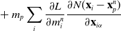 \begin{align} &\quad+m_p \sum_i \frac{\partial L}{\partial {{m_i^n}}} \frac{\partial{N(\mathbf{x}_i-\mathbf{x}_p^n)}}{\partial{\mathbf{x}_{i\alpha}}}\end{align}
Further, we have
 \begin{align} \Longrightarrow \frac{\partial L}{m_p} = \sum_i \frac{\partial L}{m_i^n}\frac{\partial m_i^n}{\partial m_p} = \sum_i \frac{\partial L}{m_i^n} N(\mathbf{\mathbf{x}_i - \mathbf{x}_p^n})\end{align}
(K, G2P) For
 $\boldsymbol\sigma_{pa}^{n}$
, we have
$\boldsymbol\sigma_{pa}^{n}$
, we have
 \begin{align}\mathbf{P}_p^{n} & = \mathbf{P}_p^{n}(\mathbf{F}_p^n, E_p, \nu_p)+\mathbf{F}_p\boldsymbol\sigma_{pa}^n \end{align}
 \begin{align} \Longrightarrow \frac{\partial L}{\partial {{\boldsymbol\sigma_{pa\alpha\beta}^{n}}}} &= \left[\frac{\partial L}{\partial {{\mathbf{P}_{elast, p}^{n}}}} \frac{\partial{{\mathbf{P}_{elast, p}^{n}}}}{\partial{{\boldsymbol\sigma_{p\alpha}^n}}}\right]_{\alpha\beta} \end{align}
 \begin{align} &= \sum_\gamma\frac{\partial L}{\partial {{\mathbf{P}_{p\gamma\beta}^{n+1}}}}\mathbf{F}_{p\gamma\alpha}^{n}. \end{align}
Here, we also note the gradients for the constitutive material constants, E and
 $\nu$
. The precise formulation of the gradients depends on the constitutive model. For the equations below, we use the Neohookean model; other gradients may be derived similarly.
$\nu$
. The precise formulation of the gradients depends on the constitutive model. For the equations below, we use the Neohookean model; other gradients may be derived similarly.
 \begin{align} \Longrightarrow \frac{\partial L}{\partial {{E_{p}^{n}}}} &= \frac{\partial L}{\partial {{\mathbf{P}_p^{n}}}} \frac{\partial{{\mathbf{P}_p^{n}}}}{\partial{{E_{p}^n}}} \end{align}
 \begin{align} &= \sum_{\beta, \gamma}\frac{\partial L}{\partial {{\mathbf{P}_{p\gamma\beta}^{n+1}}}}\frac{1}{E_p}.\end{align}
 \begin{align} \lambda_p^n &= \frac{E_p \nu_p}{(1 + \nu_p)(1 - 2 \nu_p)} \end{align}
 \begin{align} J_p^n &= \det(\mathbf{F}_{p}^{n}) \end{align}
 \begin{align} \phi_p^n &= \mathbf{P}_p^n -\lambda (J_p^n - 1) J_p^n \mathbf{F}^{-T} \end{align}
 \begin{align} \Longrightarrow \frac{\partial L}{\partial {{\nu_{p}^{n}}}} &= \frac{\partial L}{\partial {{\mathbf{P}_p^{n}}}} \frac{\partial{{\mathbf{P}_p^{n}}}}{\partial{{\nu_{p}^n}}} \end{align}
 \begin{align} &= \sum_{\beta, \gamma}\frac{\partial L}{\partial {{\mathbf{P}_{p\gamma\beta}^{n+1}}}} \left( \frac{\phi_{p\gamma\beta}^{n}}{1 + \nu_{p}} + \frac{E J_{p}^{n} (J_{p}^{n} - 1) \mathbf{F}^{-T}_{{p\beta\gamma}^{n}} (1 + 2 \nu)^{2}}{(1 - 2 \nu)^{2} (1 + \nu)^{2}} \right)\end{align}
B. Friction Projection Gradients
When there are boundary conditions:
(L, grid) For
 $\mathbf{v}_i^n$
, we have B
$\mathbf{v}_i^n$
, we have B
 \begin{align} l_{i\mathbf{n}} &= \sum_\alpha \mathbf{v}_{i\alpha} \mathbf{n}_{i\alpha}\end{align}
 \begin{align} \mathbf{v}_{i\mathbf{t}}&=\mathbf{v}_i-l_{i\mathbf{n}}\mathbf{n}_i\end{align}
 \begin{align} l_{i\mathbf{t}} &= \sqrt{\sum_\alpha \mathbf{v}_{i\mathbf{t}\alpha}^2 +\varepsilon } \end{align}
 \begin{align} \hat{\mathbf{v}}_{i\mathbf{t}}&=\frac{1}{l_{i\mathbf{t}}}\mathbf{v}_{i\mathbf{t}}\end{align}
 \begin{align} l_{i\mathbf{t}}^*&=\max\{l_{i\mathbf{t}}+c_i\min\{l_{i\mathbf{n}}, 0\}, 0\}\end{align}
 \begin{align} \mathbf{v}_i^*&=l^*_{i\mathbf{t}}\hat{\mathbf{v}}_{i\mathbf{t}}+\max\{l_{i\mathbf{n}}, 0\}\mathbf{n}_i\end{align}
 \begin{align} H(x)&: = [x\ge 0]\end{align}
 \begin{align} R&: = l_{i\mathbf{t}}+c_i\min\{l_{i\mathbf{n},0}\}\end{align}
 \begin{align} \Longrightarrow \frac{\partial L}{\partial {{l_{i\mathbf{t}}^*}}}&=\sum_\alpha \frac{\partial L}{\partial {{\mathbf{v}^*_{i\alpha}}}}{} \hat{\mathbf{v}}_{i\mathbf{t}\alpha}\end{align}
 \begin{align} \frac{\partial L}{\partial {{\hat{\mathbf{v}}_{i\mathbf{t}}}}} &= \frac{\partial L}{\partial {{\mathbf{v}^*_{i\alpha}}}}l_{i\mathbf{t}}^*\end{align}
 \begin{align} \frac{\partial L}{\partial {{l_{i\mathbf{t}}}}}&=-\frac{1}{l^{2}_{i\mathbf{t}}}\sum_\alpha \mathbf{v}_{i\mathbf{t}\alpha} \frac{\partial L}{\partial {{\hat{\mathbf{v}}_{i\mathbf{t}\alpha}}}}+\frac{\partial L}{\partial {{l_{i\mathbf{t}}^*}}}H(R)\end{align}
 \begin{align} \frac{\partial L}{\partial {{\mathbf{v}_{i\mathbf{t}\alpha}}}}&=\frac{\mathbf{v}_{i\mathbf{t}\alpha}}{l_{i\mathbf{t}}}\frac{\partial L}{\partial {{l_{i\mathbf{t}}}}}+\frac{1}{l_{i\mathbf{t}}}\frac{\partial L}{\partial {{\hat{\mathbf{v}}_{i\mathbf{t}\alpha}}}}\end{align}
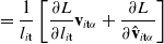 \begin{align} &=\frac{1}{l_{i\mathbf{t}}}\left[\frac{\partial L}{\partial {{l_{i\mathbf{t}}}}}\mathbf{v}_{i\mathbf{t}\alpha}+\frac{\partial L}{\partial {{\hat{\mathbf{v}}_{i\mathbf{t}\alpha}}}}\right]\end{align}
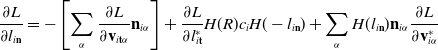 \begin{align} \frac{\partial L}{\partial {{l_{i\mathbf{n}}}}} &= -\left[\sum_\alpha \frac{\partial L}{\partial {{\mathbf{v}_{i\mathbf{t}\alpha}}}}\mathbf{n}_{i\alpha}\right]+\frac{\partial L}{\partial {{l_{i\mathbf{t}}^*}}}H(R) c_i H(-l_{i\mathbf{n}})+\sum_\alpha H(l_{i\mathbf{n}})\mathbf{n}_{i\alpha}\frac{\partial L}{\partial {{\mathbf{v}_{i\alpha}^*}}}\end{align}
 \begin{align} \frac{\partial L}{\partial {{\mathbf{v}_{i\alpha}}}} &= \frac{\partial L}{\partial {{l_{i\mathbf{n}}}}}\mathbf{n}_{i\alpha}+\frac{\partial L}{\partial {{\mathbf{v}_{i\mathbf{t}\alpha}}}}\end{align}
C. A Robot Optimization in 50 Lines of Python Code
\#Some imports we’ll want, including our building blocks and numpy and tensorflow
import tensorflow as tf
import numpy as np
from optimizers.gradient_descent_optimizer import *
from actuators.axis_aligned_pressure_actuator import *
from observors.kmeans_observor import *
from controllers.tanh_nn_controller import *
from controllable_mechanism import ControllableMechanism
from group import *
from math_tools import *
from simulation import get_bounding_box_bc
\#Set up our TF environment
sess_config = tf.ConfigProto(allow_soft_placement=True)
sess\_yconfig.gpu_options.allow_growth = True
sess_config.gpu_options.per_process_gpu_memory_fraction = 0.4
with tf.Session(config=sess_config) as sess:
\#Some constants we’ll use.
sample_density = 60 \#Each group will be 60 by 60 particles.
time, dt = 4.0, 0.005
num_steps = int(time/dt)
\#The geometric parameters of our robot
leg_width, leg_height, body_height, body_width = 0.1, 0.1, 0.1, 0.3
dim = 2 \#the dimension of the problem
\#Compose this robot from block groups of particles - what are their locs and sizes?
group_offsets = [(0, 0), (leg_width/2.0, 0), (0, leg_height),
(leg_width, leg_height),
(leg_width, leg_height + body_height/2.0),
(body_width - leg_width, leg_height),
(body_width - leg_width, 0),
(body_width - leg_width/2.0, 0)]
group_sizes = [(leg_width/2.0, leg_height), (leg_width/2.0, leg_height),
(leg_width, body_height),
(body_width - 2.0 * leg_width, body_height/2.0),
(body_width - 2.0 * leg_width, body_height/2.0),
(leg_width, body_height), (leg_width/2.0, leg_height),
(leg_width/2.0, leg_height)]
groups = []
\#Build the groups from the specifications
for i in range(len(group_offsets)):
groups.append(
Group(np.array(offset=group_offsets[i]), size=np.array(group_sizes[i]),
particle_density=np.array([sample_density, sample_density])))
\#How many particles did we allocate in total?
num_particles = sum(map(Group.get_num_particles, groups))
\#Our robot will have one a list of one observer -
\#based on the mean positions and velocities of clustered portions.
observors = [KMeansObservor(particles_to_track=list(range(num_particles)),
n_clusters=7)]
\#Allocate pressure actuators to certain groups.
\#Set the affected particles, direction, and maximum actuation
actuators = [AxisAlignedPressureActuator(get_group_particles(groups, a),
1, max_act=2.0) for a in [0,Reference Hu, Liu, Spielberg, Tenenbaum, Freeman, Wu, Rus and Matusik1,Reference Sifakis and Barbic6,Reference BarbiČ and PopoviĆ7]]
\#Create MLP with ReLUs in the hidden layers and tanh as the final activation
controller = TanhNNController(use_relu=True, hidden_layers = (64, 64))
\#What are our objective functions?
\#Maximize average forward progress in the x direction
def objective(final_state):
return -tf.reduce_mean(final_state.position[0, :])
\#Minimize running squared actuation
def running_objective(state):
return tf.linalg.norm(state.controller(state))**2
optimizer = GradientDescentOptimizer \#default Adam
\#Feed our specifications into the robot. Defaults to non-trainable design:
\#Default Young’s = 10.0, Poissons = 0.3, particle mass and volume = 1.0
cm = ControllableMechanism(sess, dim=dim, groups=groups, observors=observors,
controller = controller, actuators = actuators, optimizer = optimizer,
objectives = [(objective, 1.0)],
running_objectives = [(running_objective, 1e-8)],
use_neohookean=True)
gravity = (0, gravity_strength)
bc = get_bounding_box_bc((400, 64)) \#grid size
cm.set_world(res, bc, gravity)
\#How long will we simulate for? \#How many steps will we optimize for?
cm.initialize(dt = dt, num_steps = num_steps, num_opt_steps=100)
cm.optimize() \#Optimize over controller
D. Problem Parameters
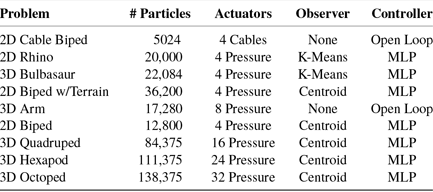


 Open access