


1. Introduction
Reactive processes in porous media play a central role in the transport, transformation and degradation of chemical and biological substances in a wide range of systems, including soils and rocks (Lichtner, Steefel & Oelkers Reference Lichtner, Steefel and Oelkers2018), engineered porous media (Perfect et al. Reference Perfect, Cheng, Kang, Bilheux, Lamanna, Gragg and Wright2014; Huang et al. Reference Huang, Wei, Gu, Kang, Lao, Li, Fan and Shou2022) and biological porous media (Khaled & Vafai Reference Khaled and Vafai2003; Goirand, Le Borgne & Lorthois Reference Goirand, Le Borgne and Lorthois2021). In many applications, reactions are driven by transport processes that bring dissolved reactants into contact (Rolle & Le Borgne Reference Rolle and Le Borgne2019; Valocchi, Bolster & Werth Reference Valocchi, Bolster and Werth2019). This reactive transport process is generally modelled using the advection dispersion reaction equation (Dentz et al. Reference Dentz, Le Borgne, Englert and Bijeljic2011), which describes mixing processes using an effective dispersion coefficient that lumps pore-scale velocity fluctuations into a single coefficient. During the last decades, there have been increasing observations of the breakdown of this model due to incomplete mixing of reactants at the pore scale (Raje & Kapoor Reference Raje and Kapoor2000; Gramling, Harvey & Meigs Reference Gramling, Harvey and Meigs2002; Klenk & Grathwohl Reference Klenk and Grathwohl2002; Battiato et al. Reference Battiato, Tartakovsky, Tartakovsky and Scheibe2009; Battiato & Tartakovsky Reference Battiato and Tartakovsky2011; De Anna et al. Reference De Anna, Jimenez-Martinez, Tabuteau, Turuban, Le Borgne, Derrien and Méheust2014).
Although different phenomenological frameworks have been proposed (Olsson & Grathwohl Reference Olsson and Grathwohl2007; Benson & Meerschaert Reference Benson and Meerschaert2008; Edery, Scher & Berkowitz Reference Edery, Scher and Berkowitz2010; Sanchez-Vila, Fernàndez-Garcia & Guadagnini Reference Sanchez-Vila, Fernàndez-Garcia and Guadagnini2010; Chiogna & Bellin Reference Chiogna and Bellin2013; Ding et al. Reference Ding, Benson, Paster and Bolster2013; Hochstetler & Kitanidis Reference Hochstetler and Kitanidis2013; Hochstetler et al. Reference Hochstetler, Rolle, Chiogna, Haberer, Grathwohl and Kitanidis2013; Porta et al. Reference Porta, Chaynikov, Thovert, Riva, Guadagnini and Adler2013; Paster, Bolster & Benson Reference Paster, Bolster and Benson2014; Bolster, Paster & Benson Reference Bolster, Paster and Benson2016; Ginn Reference Ginn2018), it is still unclear how to correctly upscale reactive processes at the Darcy scale. At the pore scale, the interplay between fluid deformations, molecular diffusion and reaction is conveniently described in a Lagrangian frame using the lamellar theory of mixing (Ranz Reference Ranz1979; Le Borgne, Dentz & Villermaux Reference Le Borgne, Dentz and Villermaux2015; Villermaux Reference Villermaux2019). The latter represents mixing interfaces as elongated lamellar structures whose stretching under the action of flow enhances mixing and reaction rates (Bandopadhyay et al. Reference Bandopadhyay, Le Borgne, Méheust and Dentz2017; Izumoto et al. Reference Izumoto, Heyman, Huisman, De Vriendt, Soulaine, Gomez, Tabuteau, Méheust and Le Borgne2023). However, it is unknown how to upscale such a pore-scale description to three-dimensional (3-D) Darcy-scale porous media. Furthermore, it is unclear how the mixing dynamics at the pore scale interacts with non-uniform flows at larger scale. A case of particular interest is converging flows in which reactive fluids flow towards each other in porous media flows (Hester et al. Reference Hester, Cardenas, Haggerty and Apte2017; Marzadri et al. Reference Marzadri, Dee, Tonina, Bellin and Tank2017; Bresciani, Kang & Lee Reference Bresciani, Kang and Lee2019; de Vriendt Reference de Vriendt2021; Izumoto et al. Reference Izumoto, Heyman, Huisman, De Vriendt, Soulaine, Gomez, Tabuteau, Méheust and Le Borgne2023). This leads to a stagnation point of the flow associated with persistent fluid compression, which can sustain reactions.
Using two-dimensional (2-D) microfluidic devices, several studies have succeeded in quantifying the evolution of concentrations of reacting species at the pore scale in mixing fronts. Reactions producing light or a fluorescent product have been used to image reaction rates in 2-D micromodels (Willingham, Werth & Valocchi Reference Willingham, Werth and Valocchi2008; De Anna et al. Reference De Anna, Jimenez-Martinez, Tabuteau, Turuban, Le Borgne, Derrien and Méheust2014; Izumoto et al. Reference Izumoto, Heyman, Huisman, De Vriendt, Soulaine, Gomez, Tabuteau, Méheust and Le Borgne2023), yielding high-resolution maps of local reaction intensity. Although 2-D porous micromodels greatly facilitate imaging at the pore scale, their mixing dynamics fundamentally differ from 3-D porous media flows, which sustain chaotic advection (Lester et al. Reference Lester, Metcalfe and Trefry2013, Reference Lester, Trefry and Metcalfe2016). Chaotic advection has recently been shown to control dilution rates and scalar gradients on the pore scale (Heyman et al. Reference Heyman, Lester, Turuban, Méheust and Le Borgne2020), affecting incomplete mixing and reactions (Sanquer et al. Reference Sanquer, Heyman, Hanna and Le Borgne2024) and fluid–solid reactions (Aquino, Le Borgne & Heyman Reference Aquino, Le Borgne and Heyman2023). Experimentally, it is particularly challenging to resolve reactive transport processes at the pore scale in 3-D porous media due to the opacity of the grains, and most studies perform measurements of the reaction rate at the outlet of columns (Ham et al. Reference Ham, Prommer, Olsson, Schotting and Grathwohl2007). Recent studies have resolved mixing-induced reactions on the pore scale using magnetic resonance imaging (Markale et al. Reference Markale, Cimmarusti, Britton and Jiménez-Martínez2021), or fluid–grain refractive index matching together with chemical reactions producing fluorescent compounds (Sanquer et al. Reference Sanquer, Heyman, Hanna and Le Borgne2024). However, these high-resolution imaging techniques are currently limited to length scales of a few tens of grains, which is not sufficient to bridge the gap to Darcy scales. Thus the impact of chaotic mixing on the large-scale reaction efficiency remains unclear. Colorimetric reactions have been used in refractive index matching media on the Darcy scale to measure the integrated mass of reaction products in an invading front (Gramling et al. Reference Gramling, Harvey and Meigs2002; Edery et al. Reference Edery, Dror, Scher and Berkowitz2015), demonstrating the persistence of the signature of incomplete mixing at large scales. These experiments were obtained in transient conditions in which a fluid flows and replaces another fluid. Such longitudinal mixing conditions are expected to be dominated by longitudinal shear rather than chaotic advection, which in steady 3-D flows occurs in the transverse direction of the flow (Lester et al. Reference Lester, Dentz, Le Borgne and de Barros2018). Hence the impact of pore-scale chaotic mixing on the Darcy-scale effective reaction reaction front properties remains unknown.
Here, we investigate the properties of the Darcy-scale reaction front of an irreversible bimolecular reaction $A+B\to C$
in steady transverse mixing fronts through porous media. In our flow cells, reactants were continuously injected by two inlets, and mixing occurred in the direction perpendicular to the mean flow direction. We combined the refractive index matching technique with chemiluminescence to map in two dimensions the effective Darcy-scale reaction rates integrated over the gap of the cell. We considered two common scenarios of mixing fronts in porous media: (i) a co-flow configuration where two reactive fluids flow in parallel in a uniform Darcy-scale flow, and (ii) a saddle flow where two reactive fluids flow towards each other in a converging flow around a stagnation point. The paper is organised as follows. We first present the theory for mixing-induced reactions in parallel and converging flows when considering diffusion or dispersion, thus neglecting the effect of incomplete mixing at the pore scale. We then compare these classical predictions with the experimental measurements, showing a significantly different evolution of the effective reaction rate with distance along the front and Péclet number because of incomplete mixing. Finally, we derive a new mechanistic model linking the pore-scale chaotic mixing to the effective reaction front properties at the Darcy scale, capturing experimental data for the range of investigated Péclet numbers, in both parallel and converging flows.
$A+B\to C$
in steady transverse mixing fronts through porous media. In our flow cells, reactants were continuously injected by two inlets, and mixing occurred in the direction perpendicular to the mean flow direction. We combined the refractive index matching technique with chemiluminescence to map in two dimensions the effective Darcy-scale reaction rates integrated over the gap of the cell. We considered two common scenarios of mixing fronts in porous media: (i) a co-flow configuration where two reactive fluids flow in parallel in a uniform Darcy-scale flow, and (ii) a saddle flow where two reactive fluids flow towards each other in a converging flow around a stagnation point. The paper is organised as follows. We first present the theory for mixing-induced reactions in parallel and converging flows when considering diffusion or dispersion, thus neglecting the effect of incomplete mixing at the pore scale. We then compare these classical predictions with the experimental measurements, showing a significantly different evolution of the effective reaction rate with distance along the front and Péclet number because of incomplete mixing. Finally, we derive a new mechanistic model linking the pore-scale chaotic mixing to the effective reaction front properties at the Darcy scale, capturing experimental data for the range of investigated Péclet numbers, in both parallel and converging flows.
2. Reactive front kinetics under diffusion and dispersion
In this section, we present the theory for bimolecular reactions $A+B\to C$
in mixing fronts when considering diffusion or hydrodynamic dispersion, for both parallel and converging flows. Deviations of experimental data from this reference model, which ignores incomplete mixing at the pore scale, will be discussed in the following sections to quantify the role of micro-scale mixing dynamics in macro-scale reactive front properties.
$A+B\to C$
in mixing fronts when considering diffusion or hydrodynamic dispersion, for both parallel and converging flows. Deviations of experimental data from this reference model, which ignores incomplete mixing at the pore scale, will be discussed in the following sections to quantify the role of micro-scale mixing dynamics in macro-scale reactive front properties.
Given a flow velocity $\boldsymbol{v}$
, the dispersion tensor
$\boldsymbol{v}$
, the dispersion tensor $\unicode{x1D63F}$
, and
$\unicode{x1D63F}$
, and $k$
the kinetic constant of a bimolecular reaction, the transport equation for the Darcy-scale concentration of the reactants
$k$
the kinetic constant of a bimolecular reaction, the transport equation for the Darcy-scale concentration of the reactants $C_A$
and
$C_A$
and $C_B$
follows:
$C_B$
follows:
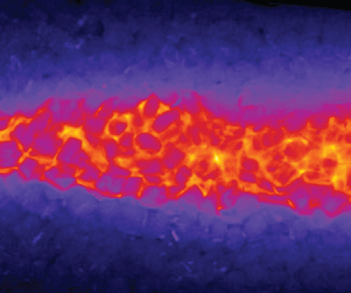
 \begin{align} \frac {\partial {C_A}}{\partial {t}} + {\boldsymbol{{v}}}\cdot \boldsymbol{\nabla} {C_A} &= \boldsymbol{\nabla} \cdot \left (\unicode{x1D63F}\,\boldsymbol{\nabla} {C_A}\right )-{k}{C_A}{C_B}, \notag \\ \frac {\partial {C_B}}{\partial {t}} + {\boldsymbol{{v}}} \cdot \boldsymbol{\nabla} {C_B} &= \boldsymbol{\nabla} \cdot \left (\unicode{x1D63F}\,\boldsymbol{\nabla} {C_B}\right )-{k}{C_A}{C_B}. \end{align}
The dispersion tensor lumps the effect of pore-scale velocity fluctuations and molecular diffusion into a single tensor, classically modelled by (Bear Reference Bear1988; Delgado Reference Delgado2007)
 \begin{equation} \unicode{x1D63F} = \left (D_{{m}} + \alpha _T\, |\boldsymbol{v}| \right )\, \unicode{x1D644}+ \left (\alpha _L-\alpha _T\right ) {\left (\boldsymbol{v} \otimes \boldsymbol{v}\right )}/{|\boldsymbol{v}|}, \end{equation}
where $\alpha _L$
and
$\alpha _L$
and $\alpha _T$
are the longitudinal and transverse dispersivities, respectively,
$\alpha _T$
are the longitudinal and transverse dispersivities, respectively, $D_{{m}}$
is the molecular diffusivity, and
$D_{{m}}$
is the molecular diffusivity, and $\unicode{x1D644}$
is the identity matrix. Two dimensionless numbers, the Péclet number
$\unicode{x1D644}$
is the identity matrix. Two dimensionless numbers, the Péclet number $Pe$
and the Damköhler number
$Pe$
and the Damköhler number $Da$
, characterise respectively the ratio of diffusion and advection times and the ratio of diffusion and reaction times. Setting
$Da$
, characterise respectively the ratio of diffusion and advection times and the ratio of diffusion and reaction times. Setting $L$
as a characteristic length scale,
$L$
as a characteristic length scale, $U$
as a characteristic velocity scale,
$U$
as a characteristic velocity scale, $C_A^0$
as the concentration of reactant
$C_A^0$
as the concentration of reactant $A$
far from the mixing front,
$A$
far from the mixing front,
 \begin{equation} Pe = \frac {U L}{D_{{m}}} \end{equation}
and
 \begin{equation} Da= \frac {k C_A^0 L^2}{D_{{m}}}. \end{equation}
We consider a mixing front in which reactant concentrations vary in the $(x,y)$
plane, with
$(x,y)$
plane, with $x$
the coordinate along the front, and
$x$
the coordinate along the front, and $y$
the coordinate in the transverse direction, and are invariant in the
$y$
the coordinate in the transverse direction, and are invariant in the $z$
direction. The two reactants are initially fully segregated (i.e.
$z$
direction. The two reactants are initially fully segregated (i.e. $(C_A,C_B)=(C_A^0,0)$
for
$(C_A,C_B)=(C_A^0,0)$
for $y\gt 0$
, and
$y\gt 0$
, and $(C_A,C_B)=(0,q C_A^0)$
for
$(C_A,C_B)=(0,q C_A^0)$
for $y\lt 0$
). We define
$y\lt 0$
). We define $q=C_B^0/C_A^0$
as the ratio of reactant concentrations on both sides of the front. The reaction rate is
$q=C_B^0/C_A^0$
as the ratio of reactant concentrations on both sides of the front. The reaction rate is $R = k C_A C_B$
. We characterise the properties of the reaction front as a function of the position
$R = k C_A C_B$
. We characterise the properties of the reaction front as a function of the position $x$
along the flow direction using three metrics: the maximum local reaction rate
$x$
along the flow direction using three metrics: the maximum local reaction rate $R_{{max}}$
defined as
$R_{{max}}$
defined as
 \begin{equation} R_{{max}}(x) = \max _y {R(x,y)}, \end{equation}
the total reaction intensity $I$
defined as the integrated reaction rate along
$I$
defined as the integrated reaction rate along $y$
,
$y$
,
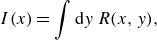 \begin{equation} I(x) = \int \text{d}y\, {R(x,y)}, \end{equation}
and the width of the reactive front $s_R$
defined from the second spatial moment of the reaction rate as
$s_R$
defined from the second spatial moment of the reaction rate as
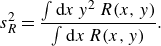 \begin{equation} s^2_R= \frac {\int \text{d}x\, y^2\, R(x,y)}{\int \text{d}x\, R(x,y)}. \end{equation}
From these definitions, $s_R \sim I/ R_{{max}}$
is expected.
$s_R \sim I/ R_{{max}}$
is expected.
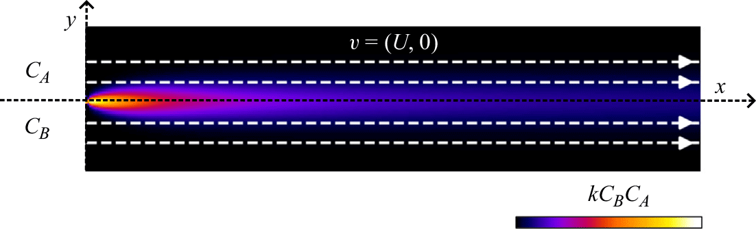
2.1. Diffusion–reaction front (co-flow)
We first consider a mixing front with two reactive fluids flowing in parallel with constant velocity $\boldsymbol{v} \equiv (U,0)$
(figure 1) and mixing transversely through diffusion only (low
$\boldsymbol{v} \equiv (U,0)$
(figure 1) and mixing transversely through diffusion only (low $Pe$
), such that (2.2) reduces to
$Pe$
), such that (2.2) reduces to $\unicode{x1D63F} \equiv D_{{m}}$
. As the flow is steady and uniform, the steady advection–diffusion problem simplifies to an unsteady diffusion problem in the Lagrangian coordinate system, where the Lagrangian time is defined by
$\unicode{x1D63F} \equiv D_{{m}}$
. As the flow is steady and uniform, the steady advection–diffusion problem simplifies to an unsteady diffusion problem in the Lagrangian coordinate system, where the Lagrangian time is defined by $t = x / U$
. From (2.1), the concentration of solute species is governed by the equations
$t = x / U$
. From (2.1), the concentration of solute species is governed by the equations
 \begin{align} \frac {\partial C_A}{\partial t} &= D_{{m}}\frac {\partial ^2 C_A}{\partial y^2}- k C_A C_B,\notag \\ \frac {\partial C_B}{\partial t} &= D_{{m}}\frac {\partial ^2 C_B}{\partial y^2}- k C_A C_B. \end{align}
Flow and boundary conditions corresponding to the co-flow mixing front. Reactants $A$
and
$A$
and $B$
are segregated and co-injected at the left-hand boundary. They flow, mix and react in the domain
$B$
are segregated and co-injected at the left-hand boundary. They flow, mix and react in the domain $x\gt 0$
. The colour scale indicates local reaction rates obtained in numerical simulations of the hydrodynamic dispersion approximation (see § A.4).
$x\gt 0$
. The colour scale indicates local reaction rates obtained in numerical simulations of the hydrodynamic dispersion approximation (see § A.4).
The properties of such a reactive front were studied by Gálfi & Rácz (Reference Gálfi and Rácz1988), Taitelbaum et al. (Reference Taitelbaum, Havlin, Kiefer, Trus and Weiss1991) and Larralde et al. (Reference Larralde, Araujo, Havlin and Stanley1992), and we recall here their main results for completeness. For an instantaneous reaction (infinite $Da$
), reactants react as soon as they meet. Thus they remain fully segregated, and the reaction intensity is driven solely by the mixing flux across the interface. For finite
$Da$
), reactants react as soon as they meet. Thus they remain fully segregated, and the reaction intensity is driven solely by the mixing flux across the interface. For finite $Da$
, two effective reaction regimes must be distinguished. At times
$Da$
, two effective reaction regimes must be distinguished. At times $t$
smaller than the characteristic reaction time
$t$
smaller than the characteristic reaction time $t_r= 1/ (C_A^0 k)$
, i.e. a distance smaller than
$t_r= 1/ (C_A^0 k)$
, i.e. a distance smaller than $t_r U$
, the reaction is slow compared to diffusion, and the front is in a reaction-limited regime. The concentration profiles of reactants can thus be approximated with the conservative concentration profiles. The characteristics of the reactive front follow typical diffusive scaling. When replacing time by position along front
$t_r U$
, the reaction is slow compared to diffusion, and the front is in a reaction-limited regime. The concentration profiles of reactants can thus be approximated with the conservative concentration profiles. The characteristics of the reactive front follow typical diffusive scaling. When replacing time by position along front $t = x / U$
, this leads to,
$t = x / U$
, this leads to,
 \begin{equation} s_r \sim L\, Pe^{-1/2} {\left ( \frac {x}{L} \right )}^{1/2}, \quad R_{{max}} \sim (C_A^0)^2 k\quad \text{and}\quad I \sim (C_A^0)^2 L k \,Pe^{-1/2} \,{\left ( \frac {x}{L} \right )}^{1/2}. \end{equation}
In contrast, at times larger than the reaction time ( $t\gt t_r$
,
$t\gt t_r$
, $x\gt t_r U$
), the front becomes mixing-limited, resulting in different scaling of the reactive front properties with distance,
$x\gt t_r U$
), the front becomes mixing-limited, resulting in different scaling of the reactive front properties with distance, $Pe$
and
$Pe$
and $D_{{m}}$
(Taitelbaum et al. Reference Taitelbaum, Havlin, Kiefer, Trus and Weiss1991). As shown in Larralde et al. (Reference Larralde, Araujo, Havlin and Stanley1992), an approximate solution can be obtained by a perturbation method that uses a spatial linearisation of the conservative profile
$D_{{m}}$
(Taitelbaum et al. Reference Taitelbaum, Havlin, Kiefer, Trus and Weiss1991). As shown in Larralde et al. (Reference Larralde, Araujo, Havlin and Stanley1992), an approximate solution can be obtained by a perturbation method that uses a spatial linearisation of the conservative profile $F=C_A-C_B$
near the front origin, while neglecting nonlinear terms (see Appendix A). This leads to
$F=C_A-C_B$
near the front origin, while neglecting nonlinear terms (see Appendix A). This leads to
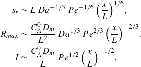 \begin{align} s_r &\sim L\, Da^{-1/3}\,Pe^{-1/6} \, {\left ( \frac {x}{L} \right )}^{1/6}, \nonumber \\ R_{{max}} &\sim \frac {C_A^0 D_{{m}}}{L^2}\, Da^{1/3}\, Pe^{2/3} \,{\left ( \frac {x}{L} \right )}^{-2/3}, \nonumber \\ I &\sim \frac {C_A^0 D_{{m}}}{L} \, Pe^{1/2} \, {\left ( \frac {x}{L} \right )}^{-1/2}. \end{align}
Note that although the reaction is fast compared to mixing in this regime, the reaction kinetics, encoded in $Da$
, still appears in the scaling laws for
$Da$
, still appears in the scaling laws for $s_r$
and
$s_r$
and $R_{{max}}$
. As
$R_{{max}}$
. As $Da$
increases, the width of the reactive zone becomes narrower because the time in which the two species can co-exist at the same location decreases. As
$Da$
increases, the width of the reactive zone becomes narrower because the time in which the two species can co-exist at the same location decreases. As $s_r$
decreases, the maximum reaction rate increases proportionally such that the product
$s_r$
decreases, the maximum reaction rate increases proportionally such that the product $s_r \times R_{{max}}$
is independent of
$s_r \times R_{{max}}$
is independent of $Da$
. This is a consequence of the independence of the reaction intensity
$Da$
. This is a consequence of the independence of the reaction intensity $I \sim s_r \times R_{{max}}$
of
$I \sim s_r \times R_{{max}}$
of $Da$
, as it is proportional to the mixing rate in the mixing-limited regime. For infinite
$Da$
, as it is proportional to the mixing rate in the mixing-limited regime. For infinite $Da$
,
$Da$
, $s_r$
goes to zero,
$s_r$
goes to zero, $R_{{max}}$
goes to infinity, and
$R_{{max}}$
goes to infinity, and $I$
remains proportional to the mixing rate. For simplicity, we did not report here the scaling with
$I$
remains proportional to the mixing rate. For simplicity, we did not report here the scaling with $q$
for the case of an asymmetric reaction in these expressions (see Appendix A for the full scaling laws).
$q$
for the case of an asymmetric reaction in these expressions (see Appendix A for the full scaling laws).
2.2. Advection–diffusion–reaction with compression (saddle flow)
We now consider the case of a reactive front in converging flows, considering a saddle flow around a stagnation point located at $(x,y)=(0,0)$
:
$(x,y)=(0,0)$
:
 \begin{equation} \boldsymbol{v} = \gamma \left (\begin{array}{c} x \\ - y \end{array} \right ), \end{equation}
where $\gamma$
is the compression rate (Haller Reference Haller2015). In this flow field, opposing flows converge and diverge at the stagnation point along directions
$\gamma$
is the compression rate (Haller Reference Haller2015). In this flow field, opposing flows converge and diverge at the stagnation point along directions $y$
and
$y$
and $x$
, respectively, leading to the formation of one stable manifold (
$x$
, respectively, leading to the formation of one stable manifold ( $\boldsymbol{y}$
) and one unstable manifold (
$\boldsymbol{y}$
) and one unstable manifold ( $\boldsymbol{x}$
) that are perpendicular to each other, and an exponential compression of fluid parcels. For this system, we define the characteristic velocity as
$\boldsymbol{x}$
) that are perpendicular to each other, and an exponential compression of fluid parcels. For this system, we define the characteristic velocity as $U=\gamma L$
and the Péclet number as
$U=\gamma L$
and the Péclet number as $Pe=\gamma L^2/D_{{m}}$
.
$Pe=\gamma L^2/D_{{m}}$
.
The saddle flow leads to the formation of a reactive front along the $x$
direction, since the two reactants are supplied in opposite directions on the
$x$
direction, since the two reactants are supplied in opposite directions on the $y$
axis (figure 2). In a Lagrangian coordinate system attached to a fluid particle travelling on the
$y$
axis (figure 2). In a Lagrangian coordinate system attached to a fluid particle travelling on the $x$
axis, the concentration of the reactant approximately follows :
$x$
axis, the concentration of the reactant approximately follows :
 \begin{equation} \frac {\partial C_A}{\partial t} - \gamma y \frac {\partial C_A}{\partial y} = D_{{m}}\frac {\partial ^2 C_A}{\partial y^2} -k C_A C_B. \end{equation}
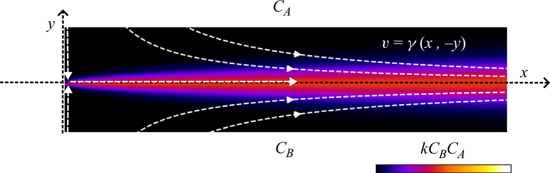
Flow and boundary conditions corresponding to the saddle mixing front. Reactants $A$
and
$A$
and $B$
are segregated and co-injected at the top and bottom boundaries, respectively. They flow, mix and react in the domain. The stagnation point is located at
$B$
are segregated and co-injected at the top and bottom boundaries, respectively. They flow, mix and react in the domain. The stagnation point is located at $(x,y)=(0,0)$
. The colour scale indicates local reaction rates obtained in numerical simulations of the hydrodynamic dispersion approximation (see § A.4).
$(x,y)=(0,0)$
. The colour scale indicates local reaction rates obtained in numerical simulations of the hydrodynamic dispersion approximation (see § A.4).
Equation (2.12) implicitly assumes that longitudinal scalar gradients are much smaller than transverse ones, which is generally the case in steady mixing front. A detailed derivation is provided in Rousseau et al. (Reference Rousseau, Izumoto, Le Borgne and Heyman2023).
As first shown by Ranz (Reference Ranz1979) in the conservative case, this equation can be solved by a change of variables that integrates the deformation of fluid elements in a Lagrangian reference system (see Villermaux (Reference Villermaux2019) for a review). Under this transformation, the advection–diffusion equation simplifies to a diffusion equation with analytical solutions. Bandopadhyay et al. (Reference Bandopadhyay, Le Borgne, Méheust and Dentz2017) and Izumoto et al. (Reference Izumoto, Heyman, Huisman, De Vriendt, Soulaine, Gomez, Tabuteau, Méheust and Le Borgne2023) have shown that reactive transport can also be studied in this Lagrangian framework by using the reaction–diffusion theory of Larralde et al. (Reference Larralde, Araujo, Havlin and Stanley1992). Two regimes can be distinguished in the saddle-flow configuration: first, a kinetic-limited regime when $\gamma \gg t_r^{-1}$
, that is, when reaction at the front is limited by the time for reaction to occur rather than by the supply of reactants; second, a mixing-limited regime for
$\gamma \gg t_r^{-1}$
, that is, when reaction at the front is limited by the time for reaction to occur rather than by the supply of reactants; second, a mixing-limited regime for $ \gamma \ll t_r^{-1}$
, where reaction is limited by the supply of reactant under the action of compression. In the kinetic-limited regime, Izumoto et al. (Reference Izumoto, Heyman, Huisman, De Vriendt, Soulaine, Gomez, Tabuteau, Méheust and Le Borgne2023) have shown that the properties of the reaction front under diffusion and compression are
$ \gamma \ll t_r^{-1}$
, where reaction is limited by the supply of reactant under the action of compression. In the kinetic-limited regime, Izumoto et al. (Reference Izumoto, Heyman, Huisman, De Vriendt, Soulaine, Gomez, Tabuteau, Méheust and Le Borgne2023) have shown that the properties of the reaction front under diffusion and compression are
 \begin{equation} s_R \sim L\, Pe^{-1/2}, \quad R_{{max}} \sim (C_A^0)^2 k\quad \text{and} \quad I \sim (C_A^0)^2 k L\, Pe^{-1/2}, \end{equation}
while in the mixing-limited regime, the front scales as
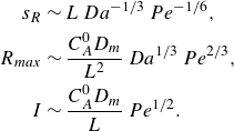 \begin{align} s_R &\sim L\, Da^{-1/3} \, Pe^{-1/6}, \nonumber \\ R_{{max}} &\sim \frac { C_A^0 D_{{m}}}{L^2}\, Da^{1/3} \, Pe^{2/3},\nonumber \\ I &\sim \frac { C_A^0 D_{{m}}}{L}\, Pe^{1/2}. \end{align}
More details on the derivation are given in Appendix A and in Izumoto et al. (Reference Izumoto, Heyman, Huisman, De Vriendt, Soulaine, Gomez, Tabuteau, Méheust and Le Borgne2023).
2.3. Advection–dispersion–reaction in porous media: co-flow
Here, we investigate how the presence of a homogeneous porous media of typical length scale $L=d$
, the grain diameter, and the resulting hydrodynamic dispersion (Delgado Reference Delgado2007) affect the properties of the reaction front for both parallel and converging flows. We assume that
$L=d$
, the grain diameter, and the resulting hydrodynamic dispersion (Delgado Reference Delgado2007) affect the properties of the reaction front for both parallel and converging flows. We assume that $\alpha _T U$
is large compared to
$\alpha _T U$
is large compared to $D_{{m}}$
(high
$D_{{m}}$
(high $Pe$
), so molecular diffusivity can be neglected in (2.2). In the co-flow scenario, the velocity is constant, so the dispersion tensor is also constant. The dispersive mixing front is therefore very similar to the diffusive one. Hence the scaling laws corresponding to diffusive transport ((2.9) and (2.10)) still hold for dispersive transport, with the molecular diffusion coefficient
$Pe$
), so molecular diffusivity can be neglected in (2.2). In the co-flow scenario, the velocity is constant, so the dispersion tensor is also constant. The dispersive mixing front is therefore very similar to the diffusive one. Hence the scaling laws corresponding to diffusive transport ((2.9) and (2.10)) still hold for dispersive transport, with the molecular diffusion coefficient $D_{{m}}$
replaced by the transverse dispersion coefficient
$D_{{m}}$
replaced by the transverse dispersion coefficient
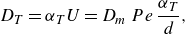 \begin{equation} D_T=\alpha _T U = D_m\, Pe\, \frac {\alpha _T}{d}, \end{equation}
the diffusive Péclet number $Pe$
replaced by a dispersive Péclet number
$Pe$
replaced by a dispersive Péclet number
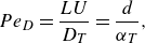 \begin{equation} Pe_D=\frac {L U}{D_T}=\frac {d}{\alpha _T}, \end{equation}
and the diffusive Damköhler number $Da$
replaced by a dispersive Damköhler number
$Da$
replaced by a dispersive Damköhler number
 \begin{equation} Da_D= \frac {Da}{Pe} \frac {d}{\alpha _T}. \end{equation}
We thus obtain in the kinetic-limited regime $x\lt t_r U$
,
$x\lt t_r U$
,
 \begin{equation} s_r \sim {\left ( {\alpha _T x}\right )}^{1/2}, \quad R_{{max}} \sim (C_A^0)^2 k \quad \text{and}\quad I \sim (C_A^0)^2 k \, {\left ( {\alpha _T x} \right )}^{1/2}, \end{equation}
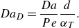
and in the mixing-limited regime $x\gt t_r U$
,
$x\gt t_r U$
,
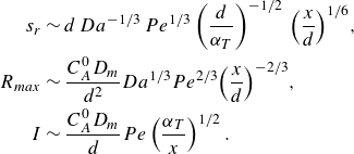 \begin{align} s_r &\sim d \, Da^{-1/3} \, Pe^{1/3} \left (\frac {d}{\alpha _T }\right )^{-1/2} \, {\left ( \frac {x}{d} \right )}^{1/6}, \nonumber \\ \nonumber R_{{max}} &\sim \frac {C_A^0 D_{{m}}}{d^2} Da^{1/3} Pe^{2/3} {\left ( \frac {x}{d} \right )}^{-2/3}, \\ I &\sim \frac {C_A^0 D_{{m}}}{d} Pe \left (\frac {\alpha _T}{x}\right )^{1/2}. \end{align}
2.4. Advection–dispersion–reaction in porous media: saddle flow
For the case of saddle flow, Rousseau et al. (Reference Rousseau, Izumoto, Le Borgne and Heyman2023) have shown that the dispersive front has a shape similar to that of the dispersive co-flow configuration, with a prefactor in the mixing width. The velocity varies spatially along the front as $\boldsymbol{v}(x,0)=(\gamma x,0)$
. Thus the transverse dispersivity is spatially dependent:
$\boldsymbol{v}(x,0)=(\gamma x,0)$
. Thus the transverse dispersivity is spatially dependent:
 \begin{equation} D_T=\alpha _T \gamma x = D_{{m}}\, Pe\, x \alpha _T/d^2 . \end{equation}
The dispersive Péclet and Damköhler numbers thus read $Pe_D= d^2 / (\alpha _T x)$
and
$Pe_D= d^2 / (\alpha _T x)$
and $Da_D = Da\, Pe^{-1}\, d^2/(\alpha _T x)$
, respectively. In the kinetic-limited regime, the diffusive scaling (2.13) thus transforms to the dispersive scaling
$Da_D = Da\, Pe^{-1}\, d^2/(\alpha _T x)$
, respectively. In the kinetic-limited regime, the diffusive scaling (2.13) thus transforms to the dispersive scaling
 \begin{equation} s_r \sim {\left ( {\alpha _T x} \right )}^{1/2}, \quad R_{{max}} \sim (C_A^0)^2 k\quad \text{and} \quad I \sim (C_A^0)^2 k {\left ( {\alpha _T x} \right )}^{1/2}. \end{equation}
In the mixing-limited regime, the diffusive scaling (2.14) transforms into the dispersive scaling
 \begin{align} s_r &\sim Da^{-1/3} Pe^{1/3} {\left ( {\alpha _T x} \right )}^{1/2}, \nonumber \\ \nonumber R_{{max}} &\sim \frac {C_A^0 D_{{m}}}{d^2} \, Da^{1/3} Pe^{2/3} , \\ I &\sim \frac {C_A^0 D_{{m}}}{d^2} \, Pe\, \left ({\alpha _T x }\right )^{1/2}, \end{align}
where $Pe=\gamma d^2/D_{{m}}$
, and
$Pe=\gamma d^2/D_{{m}}$
, and $Da$
is defined in (2.4).
$Da$
is defined in (2.4).
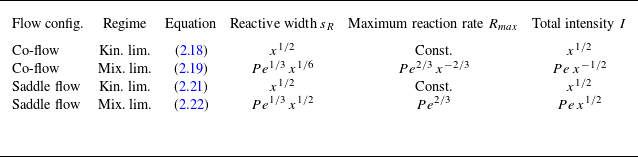
All theoretical scaling laws for reactive transport in the presence of hydrodynamic dispersion are summarised in table 1. In § A.4, we numerically validate these scaling laws for conditions close to the experiments. In the next section, we compare these analytical scaling laws with experimental data. Note that these results are derived by assuming that mixing can be modelled by hydrodynamic dispersion, hence ignoring incomplete mixing at the pore scale. Therefore, a discrepancy of these predictions with observations can be used to assess the impact of the pore-scale mixing dynamics on macroscopic reaction rates in experiments.
Summary of expected scaling laws as a function of Péclet number $Pe$
and distance
$Pe$
and distance $x$
at Darcy scale using the hydrodynamic dispersion equation, where
$x$
at Darcy scale using the hydrodynamic dispersion equation, where $x$
is the distance measured along the downstream flow direction.
$x$
is the distance measured along the downstream flow direction.
3. Experimental results
We investigated steady reactive fronts that form between two reactive fluids flowing in parallel (co-flow) or towards each other (saddle flow) in 3-D porous media. Our imaging set-up measures two-dimensional maps of the effective reaction rate integrated over several pore diameters across the cell gap. To this end, we used the principle of chemiluminescence and refractive index matching. The chemiluminescence reaction occurs through the mixing of reactants at the pore scale, producing photons that travel freely through a transparent, index-matched porous material. A camera records the total light emitted over the thickness of the cell, which corresponds to a macroscale effective reaction rate mapped across the mixing front. Experimental methods are described in the following.
3.1. Methods
3.1.1. Chemiluminescence reaction
We use the chemiluminescence of luminol (Izumoto et al. Reference Izumoto, Heyman, Huisman, De Vriendt, Soulaine, Gomez, Tabuteau, Méheust and Le Borgne2023), which involves a catalytic reaction of $\mathrm{H_2 O_2}$
with
$\mathrm{H_2 O_2}$
with $\mathrm{Co^{2+}}$
followed by an oxidation reaction of the luminol compound with
$\mathrm{Co^{2+}}$
followed by an oxidation reaction of the luminol compound with $\text{OH}\cdot$
and
$\text{OH}\cdot$
and $\mathrm{O_2}\cdot$
radicals (Uchida et al. Reference Uchida, Satoh, Yamashiro and Satoh2004). These reactions can be written as
$\mathrm{O_2}\cdot$
radicals (Uchida et al. Reference Uchida, Satoh, Yamashiro and Satoh2004). These reactions can be written as
 \begin{equation} \mathrm{luminol + H_2 O_2 + 2 OH- \xrightarrow{\,\,\,Co^2+\,\,\,} \text{3-aminophthalatedianion} + N_2 + H_2 O + {photon}} \end{equation}
luminol is oxidised to 3-aminophtalatedianion with an emission of a blue photon of wavelength $\lambda \approx 450$
nm. Such a reaction can be approximated (Matsumoto & Matsuo Reference Matsumoto and Matsuo2015) as a bimolecular reaction:
$\lambda \approx 450$
nm. Such a reaction can be approximated (Matsumoto & Matsuo Reference Matsumoto and Matsuo2015) as a bimolecular reaction:
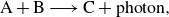 \begin{equation} \mathrm{A + B \longrightarrow C + {photon}}, \end{equation}
where $A$
and
$A$
and $B$
represent the
$B$
represent the $\mathrm{H_2 O_2}$
and the luminol species, respectively. The total reaction rate is thus directly proportional to the intensity of the emitted light. In practice, we prepared two solutions. One was a mixture of 1 mM luminol, 7 mM NaOH and 0.01 mM
$\mathrm{H_2 O_2}$
and the luminol species, respectively. The total reaction rate is thus directly proportional to the intensity of the emitted light. In practice, we prepared two solutions. One was a mixture of 1 mM luminol, 7 mM NaOH and 0.01 mM $\mathrm{CoCl_2}$
(termed luminol solution), and the other was a mixture of 0.5 mM
$\mathrm{CoCl_2}$
(termed luminol solution), and the other was a mixture of 0.5 mM $\mathrm{H_2 O_2}$
and 3.9 mM NaCl (termed
$\mathrm{H_2 O_2}$
and 3.9 mM NaCl (termed $\mathrm{H_2 O_2}$
solution). Izumoto et al. (Reference Izumoto, Heyman, Huisman, De Vriendt, Soulaine, Gomez, Tabuteau, Méheust and Le Borgne2023) have estimated the reaction constant
$\mathrm{H_2 O_2}$
solution). Izumoto et al. (Reference Izumoto, Heyman, Huisman, De Vriendt, Soulaine, Gomez, Tabuteau, Méheust and Le Borgne2023) have estimated the reaction constant $k=0.08$ $\mathrm{s^{-1}\ mM^{-1}}$
by mixing the two solutions in a beaker and measuring the intensity of light over time. This leads to the characteristic time scale
$\mathrm{s^{-1}\ mM^{-1}}$
by mixing the two solutions in a beaker and measuring the intensity of light over time. This leads to the characteristic time scale $t_r=1/(k C_0)=2.5$
s, where
$t_r=1/(k C_0)=2.5$
s, where $C_0=0.5$
mM is the concentration of luminol in the batch solution (i.e. half of the concentration of the solution before mixing). Note that after the fast reaction phase, the luminol reaction continues with a slower reaction. The light emitted from this slow reaction was subtracted from the original images by defining a threshold in the light intensity following the method of Izumoto et al. (Reference Izumoto, Heyman, Huisman, De Vriendt, Soulaine, Gomez, Tabuteau, Méheust and Le Borgne2023). Note also that the commercial
$C_0=0.5$
mM is the concentration of luminol in the batch solution (i.e. half of the concentration of the solution before mixing). Note that after the fast reaction phase, the luminol reaction continues with a slower reaction. The light emitted from this slow reaction was subtracted from the original images by defining a threshold in the light intensity following the method of Izumoto et al. (Reference Izumoto, Heyman, Huisman, De Vriendt, Soulaine, Gomez, Tabuteau, Méheust and Le Borgne2023). Note also that the commercial $\mathrm{H_2 O_2}$
solution may contain stabiliser compounds leading to a departure from the expected bimolecular kinetic. This did not occur for our 30 %
$\mathrm{H_2 O_2}$
solution may contain stabiliser compounds leading to a departure from the expected bimolecular kinetic. This did not occur for our 30 % $\mathrm{H_2 O_2}$
solution, which contained the Sigma-Aldrich stabiliser.
$\mathrm{H_2 O_2}$
solution, which contained the Sigma-Aldrich stabiliser.
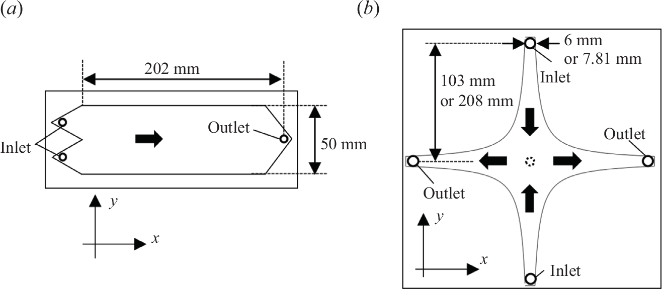
3.1.2. Flow cells
To impose the co-flow and saddle-flow conditions, we designed two flow cells. The first cell includes two inlets in two separated triangular-shaped branches (figure 3
a), leading to a co-flow configuration. By injecting two different solutions from each of the inlets, they start mixing at the edge of the separator, and they flow in parallel towards the outlet at the other side of the cell, placed 220 mm from the start of the mixing zone. The second cell has four flow branches (figure 3
b), with two inlets and two outlets. The cell boundary is chosen to be a streamline of the saddle flow (2.11), i.e. $y = \pm a/x$
, with
$y = \pm a/x$
, with $a$
a constant. The dimensions of the cells are given in figure 3. The flow cells are kept empty or filled by a transparent granular material matched to the water refractive index (fluorinated ethylene propylene, FEP) of size 2 mm. Empty cells, referred to as Hele-Shaw cells, are used to study the advection–diffusion–reaction front. They are thin (2 mm) to maintain viscous flows (low Reynolds number). Porous media cells are thicker (12 mm) to allow for the packing of a few grain diameters. Since the refractive index of FEP (1.34) is close to that of water (1.33), this allowed us to visualise an integrated image of the reaction rate over the whole cell depth. The porosity of the packed FEP was estimated to be 0.37 by comparing the saturated and unsaturated weights of the cell. Since the scalar gradients developing in co-flows and saddle flows mainly involve mixing in the direction transverse to flow (
$a$
a constant. The dimensions of the cells are given in figure 3. The flow cells are kept empty or filled by a transparent granular material matched to the water refractive index (fluorinated ethylene propylene, FEP) of size 2 mm. Empty cells, referred to as Hele-Shaw cells, are used to study the advection–diffusion–reaction front. They are thin (2 mm) to maintain viscous flows (low Reynolds number). Porous media cells are thicker (12 mm) to allow for the packing of a few grain diameters. Since the refractive index of FEP (1.34) is close to that of water (1.33), this allowed us to visualise an integrated image of the reaction rate over the whole cell depth. The porosity of the packed FEP was estimated to be 0.37 by comparing the saturated and unsaturated weights of the cell. Since the scalar gradients developing in co-flows and saddle flows mainly involve mixing in the direction transverse to flow ( $y$
), we assume that Taylor–Aris dispersion due to the Poiseuille velocity profile, which operates mainly in the direction of flow, only weakly alters mixing rates. For saddle-flow experiments, all applied compression rates were such that the characteristic compression time was larger than the reaction time,
$y$
), we assume that Taylor–Aris dispersion due to the Poiseuille velocity profile, which operates mainly in the direction of flow, only weakly alters mixing rates. For saddle-flow experiments, all applied compression rates were such that the characteristic compression time was larger than the reaction time, $\gamma ^{-1}\gt t_r$
. Hence they are in the mixing-limited regime. A summary of the experimental runs and associated parameters is provided in table 2.
$\gamma ^{-1}\gt t_r$
. Hence they are in the mixing-limited regime. A summary of the experimental runs and associated parameters is provided in table 2.
(a) Co-flow set-up and (b) saddle-flow set-up. The distance between the inlet/outlet and the stagnation point is 103 mm. For the porous medium, we used a larger cell; the distance between the inlet/outlet and the stagnation point is 208 mm. In saddle flow, $a$
is 303
$a$
is 303 $\mathrm{mm}^2$
for the Hele-Shaw cell, and 811
$\mathrm{mm}^2$
for the Hele-Shaw cell, and 811 $\mathrm{mm}^2$
for the cell for porous media. The thick arrows indicate the flow direction.
$\mathrm{mm}^2$
for the cell for porous media. The thick arrows indicate the flow direction.
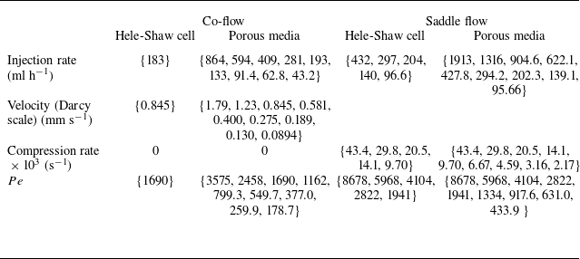
Summary of experimental runs and conditions. Constant parameters are the Damköhler number $Da=1600$
, the molecular diffusion coefficient
$Da=1600$
, the molecular diffusion coefficient $D_{{m}}=10^{-9}$ $\text{m}^2$ $\text{m}^2\ \text{s}^{-1}$
, and the characteristic length
$\text{m}^2\ \text{s}^{-1}$
, and the characteristic length $L=d=2$
mm. For co-flow,
$L=d=2$
mm. For co-flow, $Pe=U L/D_{{m}}$
. For saddle flow,
$Pe=U L/D_{{m}}$
. For saddle flow, $U=\gamma L$
, leading to
$U=\gamma L$
, leading to $Pe=\gamma L^2/D_{{m}}$
. For each flow configuration (columns) the different runs are indicated inside brackets.
$Pe=\gamma L^2/D_{{m}}$
. For each flow configuration (columns) the different runs are indicated inside brackets.
3.1.3. Protocol
Before each experiment, we filled the cell with deionised water. For experiments with porous media, we injected $\mathrm{CO_2}$
gas before filling the cell with water. Hence any trapped
$\mathrm{CO_2}$
gas before filling the cell with water. Hence any trapped $\mathrm{CO_2}$
gas dissolved in the water, and there were no remaining bubbles. Then we injected luminol and
$\mathrm{CO_2}$
gas dissolved in the water, and there were no remaining bubbles. Then we injected luminol and $\mathrm{H_2 O_2}$
solutions from two different inlets at a fixed injection rate. We imposed nine flow rates for each of the experimental configurations. The maximum Reynolds number varied between 0.18 and 3.6 for co-flow cells, and between 0.22 and 4.5 for saddle-flow cells (
$\mathrm{H_2 O_2}$
solutions from two different inlets at a fixed injection rate. We imposed nine flow rates for each of the experimental configurations. The maximum Reynolds number varied between 0.18 and 3.6 for co-flow cells, and between 0.22 and 4.5 for saddle-flow cells ( $Re=Ud/\nu$
, with
$Re=Ud/\nu$
, with $\nu =10^{-6}\ \text{m}^2\ \text{s}^{-1}$
the kinematic viscosity,
$\nu =10^{-6}\ \text{m}^2\ \text{s}^{-1}$
the kinematic viscosity, $d=2$
mm the grain size, and
$d=2$
mm the grain size, and $U=Q/A\phi$
, where
$U=Q/A\phi$
, where $Q$
is the volumetric injection rate,
$Q$
is the volumetric injection rate, $A$
is the cross-sectional area of the tank at injection, and
$A$
is the cross-sectional area of the tank at injection, and $\phi$
is the porosity). We thus assume that inertial effects are small in our experiments. For each flow rate, we waited for the front to stabilise before acquiring images with a full-frame high-sensitivity 14-bit camera (SONY alpha7s) with a macro lens (MACRO GOSS F2.8/90). The image resolution was 0.046 mm per pixel for all cases. For porous media experiments, we triplicate the experiments by repacking the FEP to obtain results independently of the specific grain packing. The images were rescaled by the bit depth of the camera to obtain the normalised reaction rate.
$\phi$
is the porosity). We thus assume that inertial effects are small in our experiments. For each flow rate, we waited for the front to stabilise before acquiring images with a full-frame high-sensitivity 14-bit camera (SONY alpha7s) with a macro lens (MACRO GOSS F2.8/90). The image resolution was 0.046 mm per pixel for all cases. For porous media experiments, we triplicate the experiments by repacking the FEP to obtain results independently of the specific grain packing. The images were rescaled by the bit depth of the camera to obtain the normalised reaction rate.
The luminol reaction can be approximated as a bimolecular reaction after subtracting light emission from the slow reaction kinetics at later times (Izumoto et al. Reference Izumoto, Heyman, Huisman, De Vriendt, Soulaine, Gomez, Tabuteau, Méheust and Le Borgne2023). We measured this weak light emission as follows. We first mixed the luminol solution and the $\mathrm{H_2 O_2}$
solution in a beaker, and then injected this solution into Hele-Shaw and porous media cells. After more than 30 minutes, we started taking images. The intensity of these pictures corresponds to the light emission from the long-lasting reaction. We subtracted these image intensities from the images taken in reactive transport experiments following the protocol of Izumoto et al. (Reference Izumoto, Heyman, Huisman, De Vriendt, Soulaine, Gomez, Tabuteau, Méheust and Le Borgne2023).
$\mathrm{H_2 O_2}$
solution in a beaker, and then injected this solution into Hele-Shaw and porous media cells. After more than 30 minutes, we started taking images. The intensity of these pictures corresponds to the light emission from the long-lasting reaction. We subtracted these image intensities from the images taken in reactive transport experiments following the protocol of Izumoto et al. (Reference Izumoto, Heyman, Huisman, De Vriendt, Soulaine, Gomez, Tabuteau, Méheust and Le Borgne2023).
We estimated the transverse width of the reactive front $s_R$
by computing the spatial standard deviation of a normalised transverse reaction rate profile. The maximum local reaction rate
$s_R$
by computing the spatial standard deviation of a normalised transverse reaction rate profile. The maximum local reaction rate $R_{{max}}$
was taken as the maximum, and the total reaction intensity
$R_{{max}}$
was taken as the maximum, and the total reaction intensity $I$
from the image intensity profile. The width was obtained experimentally by
$I$
from the image intensity profile. The width was obtained experimentally by
 \begin{equation} s_R(x)=\left (\int y^2\, P(x,y)\,{\rm d}y - \left (\int y\, P(x,y)\,{\rm d}y\right )^2\right )^{1/2}, \end{equation}
where $y$
is the transverse position, and
$y$
is the transverse position, and $P(x,y)$
is the normalised image intensity at the position
$P(x,y)$
is the normalised image intensity at the position $(x,y)$
. The maximum image intensity of the profile was chosen as
$(x,y)$
. The maximum image intensity of the profile was chosen as $R_{{max}}(x) = \max _y {P(x,y)}$
, and the image intensity was integrated over the measured line to calculate
$R_{{max}}(x) = \max _y {P(x,y)}$
, and the image intensity was integrated over the measured line to calculate $I_R(x)=\int P(x,y)\,{\rm d}y$
.
$I_R(x)=\int P(x,y)\,{\rm d}y$
.
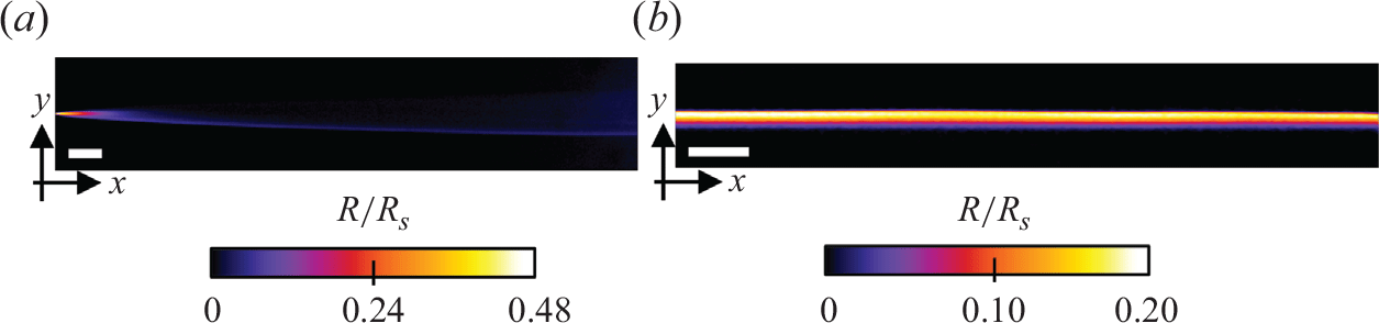
3.2. Reactive fronts in the Hele-Shaw cell
We first used Hele-Shaw cells without porous medium to confirm that the chemiluminescence reaction is a good proxy for bimolecular reactive fronts, whose theoretical behaviour is now well understood in the absence of porous media (Gálfi & Rácz Reference Gálfi and Rácz1988). In the co-flow configuration, we observe a steady reactive front that forms at the interface between the flowing reactants reactants (figure 4
a). Luminescence, which is proportional to the local reaction rate, is maximal at the entrance of the cell, and rapidly decreases as it moves downstream. The dependence of the measured reaction zone width, maximum reaction rate and total intensity with advective time (figure 5
a) is well captured by the theoretical scaling laws expected for a bimolecular reaction in a mixing-limited reactive front (2.10). We could not observe the kinetic-limited regime, which occurs at short times ( $t\lt t_r$
), probably because the cell geometry did not allow for a perfectly 2-D co-injection of reactants.
$t\lt t_r$
), probably because the cell geometry did not allow for a perfectly 2-D co-injection of reactants.
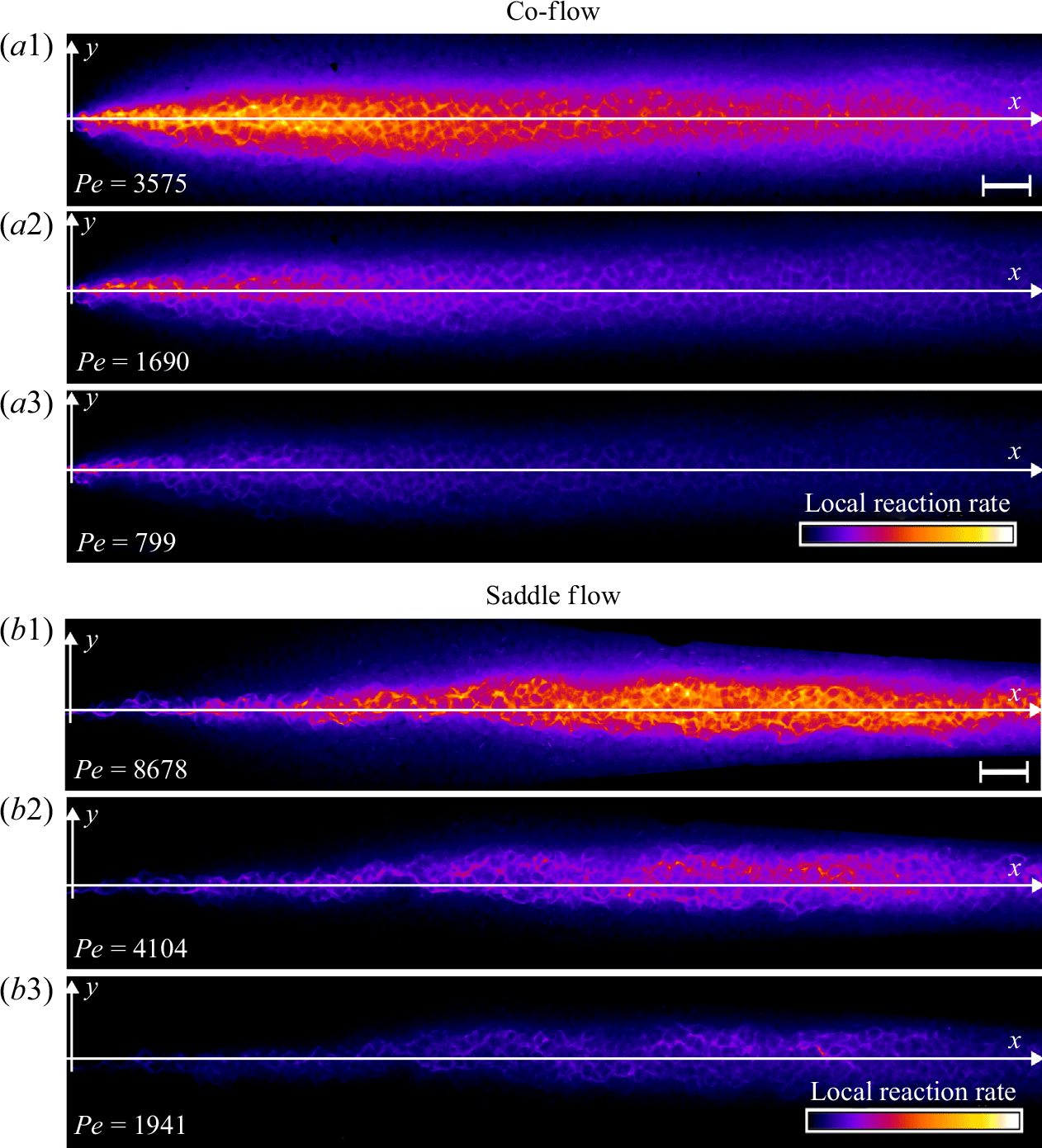
Experimental reaction rate fields in the Hele-Shaw cell for (a) the co-flow configuration ( $Pe=3575$
) and (b) the saddle-flow configuration (
$Pe=3575$
) and (b) the saddle-flow configuration ( $Pe=8678$
). Flow is from left to right. The white bar represents 10 mm. The colour scale indicates local reaction rates
$Pe=8678$
). Flow is from left to right. The white bar represents 10 mm. The colour scale indicates local reaction rates $R$
normalised by the bit depth of the camera.
$R$
normalised by the bit depth of the camera.
Experimental reaction front properties (red circles) in the Hele-Shaw cells for (a) co-flow at $Pe=1690$
and (b) saddle-flow configurations. Errors bars are calculated by taking the standard deviation over a window of length
$Pe=1690$
and (b) saddle-flow configurations. Errors bars are calculated by taking the standard deviation over a window of length $L$
. The black dashed lines show the theoretical scaling laws given by (2.10) (co-flow) and (2.14) (saddle flow). The red continuous lines are power-law fits.
$L$
. The black dashed lines show the theoretical scaling laws given by (2.10) (co-flow) and (2.14) (saddle flow). The red continuous lines are power-law fits.
In the saddle-flow configuration (figure 4
b), the reaction front is steady and invariant along the $x$
axis. In fact, the constant compression rate induced by the saddle-flow configuration maintains a fixed scale of scalar fluctuations (Rousseau et al. Reference Rousseau, Izumoto, Le Borgne and Heyman2023). We plot the characteristics of the reaction zone against the Péclet number in a window of 100 pixels centred on the stagnation point (figure 5
b). The data agree well with the scaling laws expected for the mixing-limited regime (2.14), which is expected since
$x$
axis. In fact, the constant compression rate induced by the saddle-flow configuration maintains a fixed scale of scalar fluctuations (Rousseau et al. Reference Rousseau, Izumoto, Le Borgne and Heyman2023). We plot the characteristics of the reaction zone against the Péclet number in a window of 100 pixels centred on the stagnation point (figure 5
b). The data agree well with the scaling laws expected for the mixing-limited regime (2.14), which is expected since $\gamma ^{-1}\gt t_r$
for all compression rates used experimentally. The consistency of these observations with the theoretical scaling laws (Gálfi & Rácz Reference Gálfi and Rácz1988; Larralde et al. Reference Larralde, Araujo, Havlin and Stanley1992) confirms that the chemiluminescence reaction is well approximated by a bimolecular reaction.
$\gamma ^{-1}\gt t_r$
for all compression rates used experimentally. The consistency of these observations with the theoretical scaling laws (Gálfi & Rácz Reference Gálfi and Rácz1988; Larralde et al. Reference Larralde, Araujo, Havlin and Stanley1992) confirms that the chemiluminescence reaction is well approximated by a bimolecular reaction.
3.3. Steady reactive fronts in porous media
Experimental images of reactive fronts obtained in porous media cells in co-flow and saddle-flow configurations are shown in figure 6 for increasing Péclet numbers. The presence of grains clearly enhances the transverse spreading of the reactive zone compared to the open flow case (figure 4). In contrast to the Hele-Shaw cell, the reactive mixing interface that forms in the saddle flow in porous media broadens with $x$
(figure 6
b), since the dispersion coefficient increases with
$x$
(figure 6
b), since the dispersion coefficient increases with $x$
. This broadening was also observed in conservative transport experiments (Rousseau et al. Reference Rousseau, Izumoto, Le Borgne and Heyman2023). We present in figure 7 the characteristics of the reactive front and its dependence on the distance
$x$
. This broadening was also observed in conservative transport experiments (Rousseau et al. Reference Rousseau, Izumoto, Le Borgne and Heyman2023). We present in figure 7 the characteristics of the reactive front and its dependence on the distance $x$
for the co-flow and for the saddle flow. In co-flow, we normalise the distance by the characteristic reaction distance
$x$
for the co-flow and for the saddle flow. In co-flow, we normalise the distance by the characteristic reaction distance $x_r=U/t_r$
to highlight the two different regimes in space. For saddle flow, we normalise
$x_r=U/t_r$
to highlight the two different regimes in space. For saddle flow, we normalise $x$
by grain size since there is only one regime in space. We averaged these characteristics over triplicate experiments with different grain packings.
$x$
by grain size since there is only one regime in space. We averaged these characteristics over triplicate experiments with different grain packings.
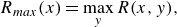
Normalised steady-state reaction rate fields for (a) co-flow and (b) saddle flow, obtained from chemiluminescence experiments in porous media. The reaction rate is normalised by the maximum reaction rate at the highest $Pe$
for each configuration. The white scale bar has length 10 mm. The porosity appears as dark patches in the mixing front. For (a), the left-hand edge corresponds to the start of mixing and for (b), the left-hand edge corresponds to the stagnation point.
$Pe$
for each configuration. The white scale bar has length 10 mm. The porosity appears as dark patches in the mixing front. For (a), the left-hand edge corresponds to the start of mixing and for (b), the left-hand edge corresponds to the stagnation point.
Reactive mixing properties measured in porous media. (a) The reaction front properties over distance normalised by the characteristic reaction distance $x_r$
in co-flow porous media experiments, showing (a1) reaction intensity, (a2) maximum reaction rate, and (a3) reaction width. The dashed lines show the scaling laws expected from the hydrodynamic dispersion theory (2.18), (2.19). (b) Reaction front properties over distance normalised by the grain diameter in saddle-flow porous media experiments, showing (b1) reaction intensity, (b2) maximum reaction rate, and (b3) reaction width. The dashed lines show the scaling expected from the hydrodynamic dispersion theory (2.22). Continuous lines show the fit to the data. The error margin is estimated from the minimum and maximum envelope of the three experimental replicates obtained with different packing realisations.
$x_r$
in co-flow porous media experiments, showing (a1) reaction intensity, (a2) maximum reaction rate, and (a3) reaction width. The dashed lines show the scaling laws expected from the hydrodynamic dispersion theory (2.18), (2.19). (b) Reaction front properties over distance normalised by the grain diameter in saddle-flow porous media experiments, showing (b1) reaction intensity, (b2) maximum reaction rate, and (b3) reaction width. The dashed lines show the scaling expected from the hydrodynamic dispersion theory (2.22). Continuous lines show the fit to the data. The error margin is estimated from the minimum and maximum envelope of the three experimental replicates obtained with different packing realisations.
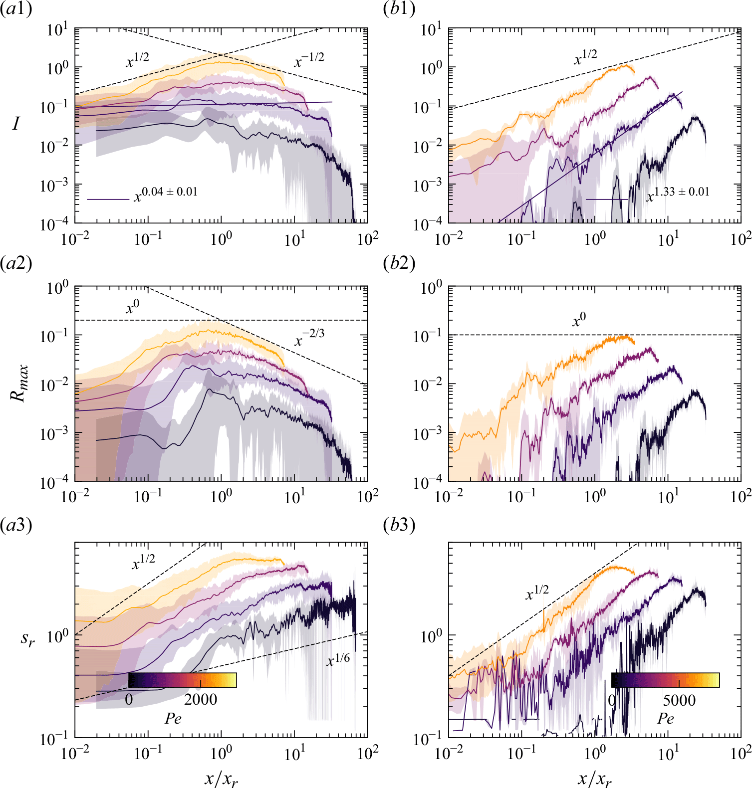
For co-flow experiments, we observe first a kinetic-limited regime, where the reaction intensity $I$
increases with distance and then, further downstream, a mixing-limited regime, where
$I$
increases with distance and then, further downstream, a mixing-limited regime, where $I$
decays (figure 7
a1). The transition distance between the two regimes is obtained at
$I$
decays (figure 7
a1). The transition distance between the two regimes is obtained at $x\approx x_r$
. In the kinetic-limited regime,
$x\approx x_r$
. In the kinetic-limited regime, $R_{{max}}$
and
$R_{{max}}$
and $I$
increase faster than predicted by the hydrodynamic dispersion theory (2.19). In the mixing-limited regime (
$I$
increase faster than predicted by the hydrodynamic dispersion theory (2.19). In the mixing-limited regime ( $x\gt x_r$
), the decay of
$x\gt x_r$
), the decay of $R_{{max}}$
and
$R_{{max}}$
and $I$
is closer to the hydrodynamic dispersion model (2.10). For saddle-flow experiments, the evolution of
$I$
is closer to the hydrodynamic dispersion model (2.10). For saddle-flow experiments, the evolution of $R_{{max}}$
and
$R_{{max}}$
and $I$
with distance is also significantly faster than predicted by the hydrodynamic dispersion theory for the mixing-limited regime (2.22).
$I$
with distance is also significantly faster than predicted by the hydrodynamic dispersion theory for the mixing-limited regime (2.22).
Interestingly, the measured reactive mixing width $s_R$
in both co-flow and saddle flows in the presence of porous media approximately follows the hydrodynamic dispersion predictions (2.18), (2.19), (2.22). This suggests that the hydrodynamic dispersion theory provides a robust framework to predict the spatial extent of the mixing fronts, as observed by Rousseau et al. (Reference Rousseau, Izumoto, Le Borgne and Heyman2023) for conservative mixing, although it does not capture actual mixing and reaction rates.
$s_R$
in both co-flow and saddle flows in the presence of porous media approximately follows the hydrodynamic dispersion predictions (2.18), (2.19), (2.22). This suggests that the hydrodynamic dispersion theory provides a robust framework to predict the spatial extent of the mixing fronts, as observed by Rousseau et al. (Reference Rousseau, Izumoto, Le Borgne and Heyman2023) for conservative mixing, although it does not capture actual mixing and reaction rates.
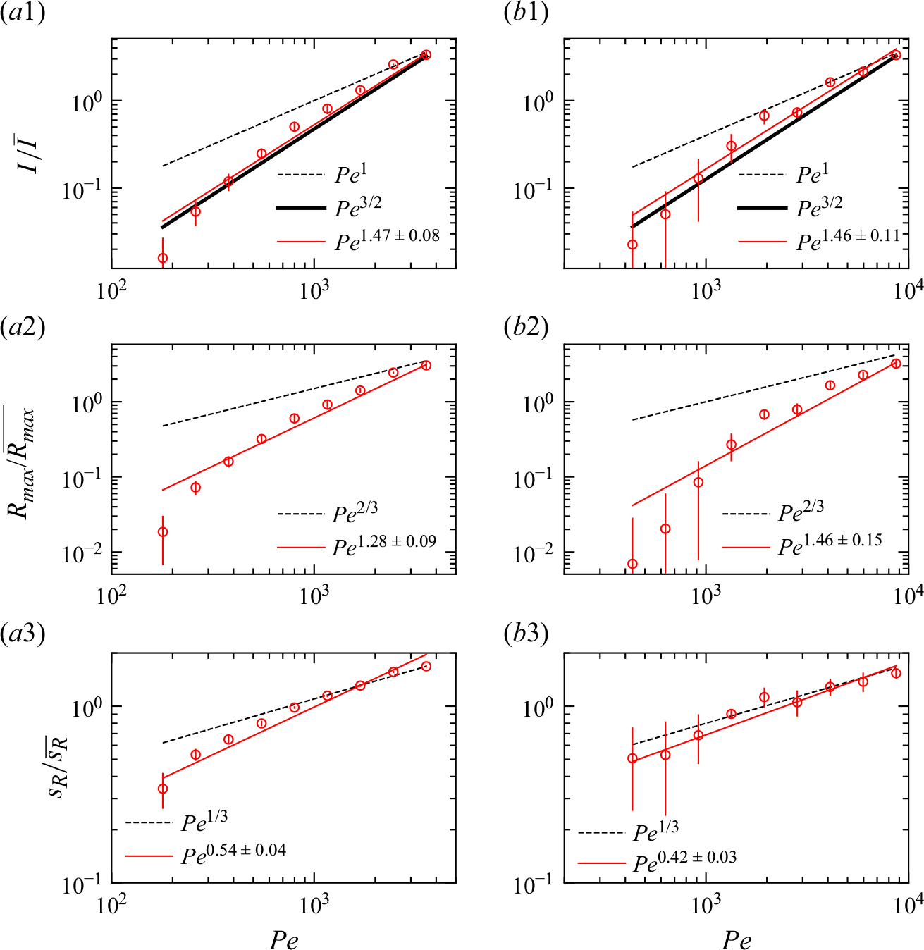
We plot the properties of the experimental reaction front as a function $Pe$
measured at
$Pe$
measured at $x=10 d$
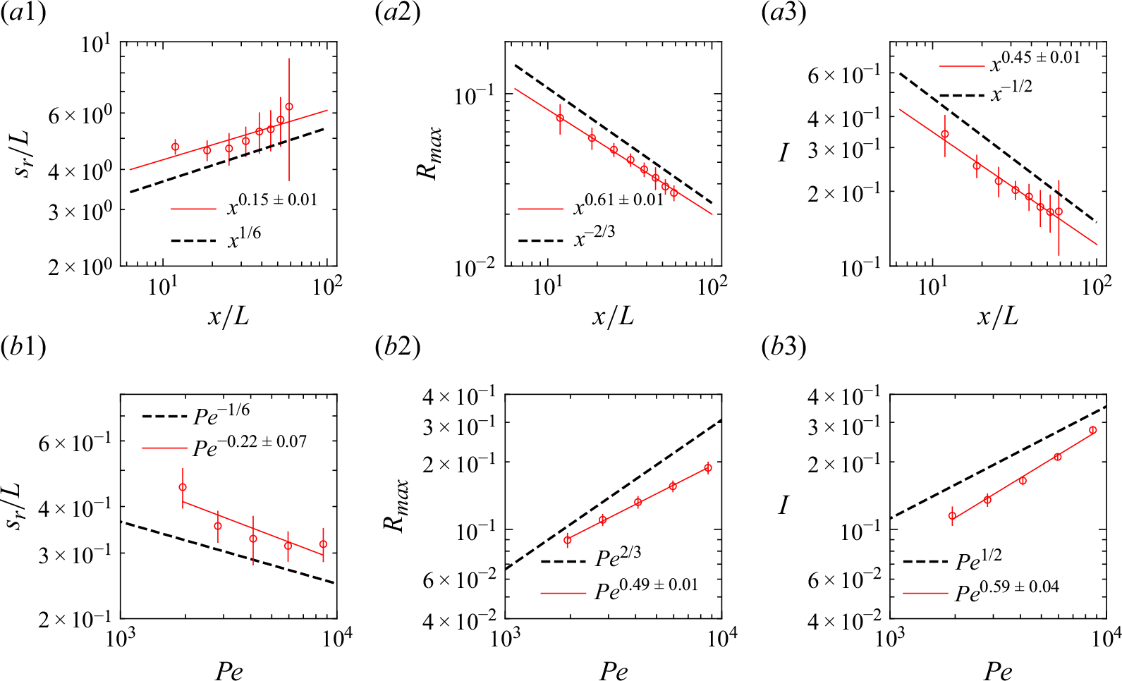
in figure 8. At this position, all experiments are in the mixing-limited regime. For the intensity of the reaction front intensity (figure 8
a1,b1) and the maximum reaction rate (figure 8
a2,b2), the evolution with the Péclet number is stronger than predicted by the hydrodynamic dispersion theory. This discrepancy suggests that incomplete pore-scale mixing plays an important role, as discussed in the following. Note that the evolution of the reactive width with the Péclet number (figure 8
a3,b3) is consistent with the scaling predicted by hydrodynamic dispersion, since this spatially integrated measure is not modified by the presence of pore-scale gradients, as also found in conservative experiments (Rousseau et al. Reference Rousseau, Izumoto, Le Borgne and Heyman2023) .
$x=10 d$
in figure 8. At this position, all experiments are in the mixing-limited regime. For the intensity of the reaction front intensity (figure 8
a1,b1) and the maximum reaction rate (figure 8
a2,b2), the evolution with the Péclet number is stronger than predicted by the hydrodynamic dispersion theory. This discrepancy suggests that incomplete pore-scale mixing plays an important role, as discussed in the following. Note that the evolution of the reactive width with the Péclet number (figure 8
a3,b3) is consistent with the scaling predicted by hydrodynamic dispersion, since this spatially integrated measure is not modified by the presence of pore-scale gradients, as also found in conservative experiments (Rousseau et al. Reference Rousseau, Izumoto, Le Borgne and Heyman2023) .
The reaction front properties as a function of $Pe$
for porous media experiments measured at fixed distance
$Pe$
for porous media experiments measured at fixed distance $x = 20d \pm 10d$
. (a) Co-flow porous media with (a1) reaction intensity, (a2) maximum reaction rate, and (a3) reaction width. (b) Saddle-flow porous media with (b1) reaction intensity, (b2) maximum reaction rate, and (b3) reaction width. Error bars are estimated from the variability of reaction front properties at various distances between
$x = 20d \pm 10d$
. (a) Co-flow porous media with (a1) reaction intensity, (a2) maximum reaction rate, and (a3) reaction width. (b) Saddle-flow porous media with (b1) reaction intensity, (b2) maximum reaction rate, and (b3) reaction width. Error bars are estimated from the variability of reaction front properties at various distances between $x=10d$
and
$x=10d$
and $x=30d$
. The 95 % confidence interval is shown. Note that the width at the lower two
$x=30d$
. The 95 % confidence interval is shown. Note that the width at the lower two $Pe$
values, and the maximum reaction rate and intensity at the lowest
$Pe$
values, and the maximum reaction rate and intensity at the lowest $Pe$
, could not be obtained because of the small image intensity. The dashed lines show the scaling expected from the hydrodynamic dispersion theory ((2.18), (2.19) and (2.22)). The scaling of the effective reaction intensity
$Pe$
, could not be obtained because of the small image intensity. The dashed lines show the scaling expected from the hydrodynamic dispersion theory ((2.18), (2.19) and (2.22)). The scaling of the effective reaction intensity $I$
predicted by the micro-scale mixing theory ((4.16) and (4.20)) is shown as thick continuous lines.
$I$
predicted by the micro-scale mixing theory ((4.16) and (4.20)) is shown as thick continuous lines.
4. Discussion
Experimental observations show that reaction rates in mixing fronts under flow in porous media largely depart from those predicted by the hydrodynamic dispersion framework. In this section, we discuss the origin of this discrepancy and investigate the role played by pore-scale chaotic advection (Lester, Metcalfe & Trefry Reference Lester, Metcalfe and Trefry2013; Heyman et al. Reference Heyman, Lester, Turuban, Méheust and Le Borgne2020), which is expected to sustain chemical gradients and drives the rate of mixing at the pore scale. We focus on the total intensity of the reaction $I$
along the reactive front, because it is a robust integrated measure of effective reaction rates.
$I$
along the reactive front, because it is a robust integrated measure of effective reaction rates.
4.1. Stretching-enhanced reactive front kinetics under co-flow
At the pore scale, we define the mixing interface as the isoconcentration surface where $C_A=C_B$
. This surface coincides with the conservative isoconcentration surface
$C_A=C_B$
. This surface coincides with the conservative isoconcentration surface $F=0$
, with the conservative component
$F=0$
, with the conservative component $F={C_A-C_B}$
. In a given cross-section perpendicular to the flow (figure 9), the length of this interface results from a balance between stretching, which continuously deforms the interface (figure 9) and aggregation/dilution, which reduces its length by merging and diluting the stretched sections of the front (Le Borgne, Dentz & Villermaux Reference Le Borgne, Dentz and Villermaux2013; Villermaux Reference Villermaux2018, Reference Villermaux2019).
$F={C_A-C_B}$
. In a given cross-section perpendicular to the flow (figure 9), the length of this interface results from a balance between stretching, which continuously deforms the interface (figure 9) and aggregation/dilution, which reduces its length by merging and diluting the stretched sections of the front (Le Borgne, Dentz & Villermaux Reference Le Borgne, Dentz and Villermaux2013; Villermaux Reference Villermaux2018, Reference Villermaux2019).
Sketch of the micro-scale mixing interface between reactants A and B. (a) Starting from a given mixing interface (black line), fluid stretching leads to an incremental elongation of the interface (red line). The latter is balanced by two main processes that contribute to the reduction of the interface. The first is dilution, which describes the decay of concentration of an isolated lamella of A into the B side (or the opposite). The second is aggregation, which describes the overlap of difference sections of the front. (b) Considering a lamella of A being stretched into the B side, the section of width equal to the Batchelor scale dilutes exponentially, leading to a receding of the interface and thus a flux of A into the B side.
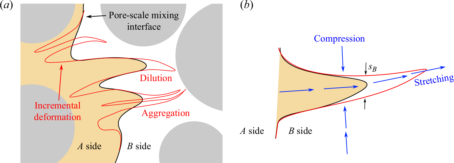
Due to stretching, the mixing front forms an ensemble of lamellae that are elongated in one direction and compressed in the other (figure 9
a). The elongation of a lamella is defined as $\rho (t)=\ell (t)/\ell _0$
, where
$\rho (t)=\ell (t)/\ell _0$
, where $\ell _0$
and
$\ell _0$
and $\ell (t)$
are the initial and final lengths of the lamella, respectively. The chaotic nature of pore-scale stretching (Heyman et al. Reference Heyman, Lester, Turuban, Méheust and Le Borgne2020; Souzy et al. Reference Souzy, Lhuissier, Méheust, Le Borgne and Metzger2020) implies that this elongation should be exponential, e.g.
$\ell (t)$
are the initial and final lengths of the lamella, respectively. The chaotic nature of pore-scale stretching (Heyman et al. Reference Heyman, Lester, Turuban, Méheust and Le Borgne2020; Souzy et al. Reference Souzy, Lhuissier, Méheust, Le Borgne and Metzger2020) implies that this elongation should be exponential, e.g. $\rho ={\rm e}^{\lambda t}$
, with
$\rho ={\rm e}^{\lambda t}$
, with
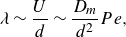 \begin{equation} \lambda \sim \frac {U}{d} \sim \frac {D_m}{d^2} Pe, \end{equation}
the Lyapunov exponent. At pore scale, the thickness of lamella $s$
is reduced by compression and enhanced by diffusion, according to
$s$
is reduced by compression and enhanced by diffusion, according to
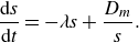 \begin{equation} \frac {\textrm{d} s}{\textrm{d} t} = -\lambda s + \frac {D_{{m}}}{s}. \end{equation}
When compression and diffusion balance each other, i.e. when the temporal derivative on the right-hand side of (4.2) is zero, the lamellar width converges to the Batchelor scale (Batchelor, Howells & Townsend Reference Batchelor, Howells and Townsend1959),
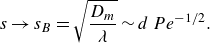 \begin{equation} s\to s_B = \sqrt {\frac {D_m}{\lambda }} \sim d \, Pe^{-1/2}. \end{equation}
This equilibrium is achieved at the mixing time (Villermaux Reference Villermaux2019)
 \begin{equation} t_m \sim \frac {\log Pe}{2 \lambda }, \end{equation}
which is obtained when the lamella width reaches the Batchelor scale by compression from the initial width, $s_0\, {\rm e}^{-\lambda t_m}=s_B$
.
$s_0\, {\rm e}^{-\lambda t_m}=s_B$
.
After mixing time, further elongation of lamellae of constant width $s_B$
in a finite-size domain implies that they overlap and aggregate, limiting the growth of the total interface length (figure 9
a). Furthermore, lamellae of
$s_B$
in a finite-size domain implies that they overlap and aggregate, limiting the growth of the total interface length (figure 9
a). Furthermore, lamellae of $A$
that are stretched in the
$A$
that are stretched in the $B$
domain (or
$B$
domain (or $B$
into
$B$
into $A$
) start to dilute exponentially, leading to receding of the interface after an incremental deformation (figure 9
b). In this regime, the balance between constant stretching and destruction of the interface thus leads to a saturation of the front elongation to a maximum value
$A$
) start to dilute exponentially, leading to receding of the interface after an incremental deformation (figure 9
b). In this regime, the balance between constant stretching and destruction of the interface thus leads to a saturation of the front elongation to a maximum value $\rho _m$
equal to the elongation at the mixing time (Villermaux Reference Villermaux2018):
$\rho _m$
equal to the elongation at the mixing time (Villermaux Reference Villermaux2018):
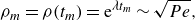 \begin{equation} \rho _m=\rho (t_m)={\rm e}^{\lambda t_m} \sim \sqrt {Pe}, \end{equation}
where we have used (4.4) and (4.1).
We first consider an element of the interface that is stretched in the $B$
domain at constant stretching rate (figure 9
b). After the mixing time, the mixing interface reaches a steady state, and the tip of the lamella, of width equal to the Batchelor scale, dilutes exponentially. This dilution leads to a flux of
$B$
domain at constant stretching rate (figure 9
b). After the mixing time, the mixing interface reaches a steady state, and the tip of the lamella, of width equal to the Batchelor scale, dilutes exponentially. This dilution leads to a flux of $A$
to the
$A$
to the $B$
side, which is proportional to the stretching rate:
$B$
side, which is proportional to the stretching rate:
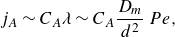 \begin{equation} j_A \sim C_A \lambda \sim C_A \frac {D_m}{d^2}\, Pe, \end{equation}
where $C_A$
is the characteristic concentration of
$C_A$
is the characteristic concentration of $A$
. When the mixing interface reaches a steady length
$A$
. When the mixing interface reaches a steady length $\rho _m$
, it is composed of a characteristic number of elongated elements
$\rho _m$
, it is composed of a characteristic number of elongated elements $n \propto {\rho _m}/{L}$
, with
$n \propto {\rho _m}/{L}$
, with $L$
the domain size. Using (4.5), we estimate
$L$
the domain size. Using (4.5), we estimate
 \begin{equation} n = \beta \sqrt {Pe}, \end{equation}
with $\beta$
a constant prefactor to be determined. The total flux across the interface due to the dilution of these stretched segments of the interface is thus
$\beta$
a constant prefactor to be determined. The total flux across the interface due to the dilution of these stretched segments of the interface is thus
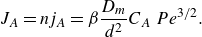 \begin{equation} J_A = n j_A = \beta \frac {D_m}{d^2} C_A\, Pe^{3/2}. \end{equation}
Initially, reactants are fully segregated, and $C_A$
and
$C_A$
and $C_B$
remain close to their initial concentrations
$C_B$
remain close to their initial concentrations $C_A^0$
and
$C_A^0$
and $q C_A^0$
. At a further distance downstream, called
$q C_A^0$
. At a further distance downstream, called $x_\varDelta$
, dispersion inevitably smooths scalar gradients at the interface such that
$x_\varDelta$
, dispersion inevitably smooths scalar gradients at the interface such that $C_A\lt C_A^0$
, limiting the flux of
$C_A\lt C_A^0$
, limiting the flux of $A$
in (4.6), and equivalently for the flux of
$A$
in (4.6), and equivalently for the flux of $B$
. We focus here on the first regime, where
$B$
. We focus here on the first regime, where $x\lt x_{\varDelta }$
and
$x\lt x_{\varDelta }$
and $C_A \approx C_A^0$
(
$C_A \approx C_A^0$
( $C_B \approx q C_A^0$
), which covers a large part of our measurements. Note that in the case of fast reactions (large Damköhler numbers), reactions occur mostly at the mixing interface where concentrations are similar. Here, we consider the general case of arbitrary Damköhler numbers where reactions can be slow compared to mixing rates. In this case, reactions also occur further away from the mixing interface. On the
$C_B \approx q C_A^0$
), which covers a large part of our measurements. Note that in the case of fast reactions (large Damköhler numbers), reactions occur mostly at the mixing interface where concentrations are similar. Here, we consider the general case of arbitrary Damköhler numbers where reactions can be slow compared to mixing rates. In this case, reactions also occur further away from the mixing interface. On the $B$
side, the concentration of
$B$
side, the concentration of $A$
becomes rapidly much smaller than that of
$A$
becomes rapidly much smaller than that of $B$
as it is diluted by stretching-enhanced diffusion. The evolution of the mass of
$B$
as it is diluted by stretching-enhanced diffusion. The evolution of the mass of $A$
on the
$A$
on the $B$
side, denoted
$B$
side, denoted $m_{A|B}$
, can thus be approximated as a first-order reaction process:
$m_{A|B}$
, can thus be approximated as a first-order reaction process:
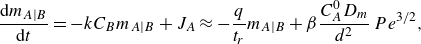 \begin{equation} \frac {{\rm d}m_{A|B}}{{\rm d}t}= -k C_B m_{A|B} + J_A \approx - \frac {q}{t_r} m_{A|B} + \beta \frac {C_A^0 D_m}{d^2}\, Pe^{3/2}, \end{equation}
where we used $C_B \approx q C_A^0$
for
$C_B \approx q C_A^0$
for $x\lt x_{\varDelta }$
and for the general case of an asymmetric reaction front. This equation leads to
$x\lt x_{\varDelta }$
and for the general case of an asymmetric reaction front. This equation leads to
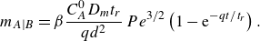 \begin{equation} m_{A|B}=\beta \frac {C_A^0 D_{{m}} t_r }{q d^2}\, Pe^{3/2} \left ( 1-{\rm e}^{- q t/t_r} \right ) . \end{equation}
Similar arguments can be used to estimate $m_{B|A}$
, leading to
$m_{B|A}$
, leading to
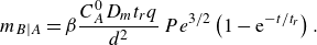 \begin{equation} m_{B|A}= \beta \frac {C_A^0 D_{{m}} t_r q}{d^2}\, Pe^{3/2} \left ( 1-{\rm e}^{- t/t_r} \right ) . \end{equation}
Thus the total reaction intensity developing on the two sides of the mixing front is
 \begin{equation} I = k C_B^0 m_{A|B} + k C_A^0 m_{B|A} = \beta q \frac {C_A^0 D_{{m}}}{d^2}\, Pe^{3/2} \left ( 2-{\rm e}^{- t/t_r}-{\rm e}^{- q t/t_r} \right ). \end{equation}
Replacing $t$
by
$t$
by $x/U$
and using the definitions of
$x/U$
and using the definitions of $Pe$
and
$Pe$
and $Da$
(see (2.3) and (2.4)), the last equation is
$Da$
(see (2.3) and (2.4)), the last equation is
 \begin{equation} I =\beta q \frac {C_A^0 D_{{m}}}{d^2}\, Pe^{3/2} \left ( 2-\exp \left (- \frac {Da}{Pe}\frac {x}{d} \right ) -\exp \left (- q\frac {Da}{Pe}\frac {x}{d} \right ) \right ). \end{equation}
This equation predicts a linear growth of reaction intensity followed by a plateau (figure 10
a). In the kinetic-limited regime $t \ll t_r$
, the consumption rate is much smaller than the mixing flux. Hence the mass of
$t \ll t_r$
, the consumption rate is much smaller than the mixing flux. Hence the mass of $A$
in the
$A$
in the $B$
domain grows linearly as
$B$
domain grows linearly as
 \begin{equation} m_{A|B} = J_A t, \end{equation}
which corresponds to a Taylor expansion of (4.11) at small times $t \ll t_r$
. The intensity of the reaction is thus
$t \ll t_r$
. The intensity of the reaction is thus
 \begin{equation} I = \beta q \frac { (1+q) D_{{m}} C_A^0 }{d^2}\, Da\, Pe^{3/2}\, \frac {t}{t_r} \sim \beta q \frac { (1+q) D_{{m}} C_A^0 }{d^2}\, Da\, Pe^{1/2} \,\frac {x}{d}. \end{equation}
In the mixing-limited regime $t \gg t_r$
, the reaction is fast compared to mixing, and the reaction intensity reaches a constant:
$t \gg t_r$
, the reaction is fast compared to mixing, and the reaction intensity reaches a constant:
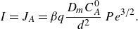 \begin{equation} I = J_A = \beta q \frac {D_{{m}} C_A^0}{d^2}\, Pe^{3/2}. \end{equation}
This constant is proportional to the flux of the solute across the mixing front, and corresponds to the asymptotic limit of (4.13) at large times.
Comparison of theoretical predictions for the mixing model (dashed lines, (4.13) and (4.20)) and the dispersive model (dotted lines, (2.18), (2.19) and (2.22)) with data (solid lines) for the reaction intensity versus distance for (a) the co-flow and (b) the saddle flow. Independent parameters are $Da=1600$
,
$Da=1600$
, $D_{{m}}=10^{-9}$
m
$D_{{m}}=10^{-9}$
m $^2$
s−1,
$^2$
s−1, $C_A^0=1$
mM, and
$C_A^0=1$
mM, and $q=2$
. Prefactors used for fitting models are 0.2 (dispersive co-flow),
$q=2$
. Prefactors used for fitting models are 0.2 (dispersive co-flow), $5\times 10^{-3}$
(dispersive saddle flow),
$5\times 10^{-3}$
(dispersive saddle flow), $\beta = 2 \times 10^{-2}$
(mixing model co-flow) and
$\beta = 2 \times 10^{-2}$
(mixing model co-flow) and $\beta ' = 3\times 10^{-5}$
(mixing model saddle flow).
$\beta ' = 3\times 10^{-5}$
(mixing model saddle flow).
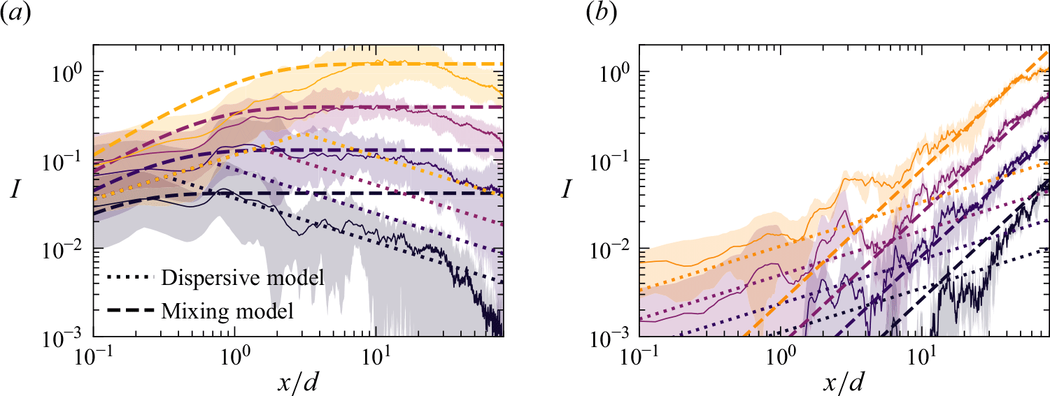
The model of (4.13) is in relatively good agreement with experimental data for the range of distances and Péclet numbers considered (figure 10
a). The prefactor $\beta$
in (4.7) is the unique fitting parameter of the model, and is the same for all experiment runs. As a reference, we also plot in figure 10(a) the prediction of the dispersion model, whose parameters are determined by a fit to the lowest Péclet number. Although the dispersion model captures the data relatively well for the lowest Péclet number, it diverges significantly for the largest Péclet numbers, with up to one order of magnitude difference from the data. In contrast, the mixing model captures the initial growth followed by a plateau observed for the evolution of the reaction intensity with distance (figure 10
a), and the dependence of the reaction intensity and reaction maximum with the Péclet number (figure 8
a1,a2). Thus it provides a mechanism to quantify incomplete mixing at the pore scale and explain the failure of the hydrodynamic dispersion model. The agreement is less good for the lowest Péclet number (
$\beta$
in (4.7) is the unique fitting parameter of the model, and is the same for all experiment runs. As a reference, we also plot in figure 10(a) the prediction of the dispersion model, whose parameters are determined by a fit to the lowest Péclet number. Although the dispersion model captures the data relatively well for the lowest Péclet number, it diverges significantly for the largest Péclet numbers, with up to one order of magnitude difference from the data. In contrast, the mixing model captures the initial growth followed by a plateau observed for the evolution of the reaction intensity with distance (figure 10
a), and the dependence of the reaction intensity and reaction maximum with the Péclet number (figure 8
a1,a2). Thus it provides a mechanism to quantify incomplete mixing at the pore scale and explain the failure of the hydrodynamic dispersion model. The agreement is less good for the lowest Péclet number ( $Pe=179$
), for which the model tends to overestimate reaction intensities. At low Péclet number, the fluctuation scale (set by the Batchelor scale) reaches the grain size, and incomplete mixing is expected to be less significant. Using the estimate of the Lyapunov exponent
$Pe=179$
), for which the model tends to overestimate reaction intensities. At low Péclet number, the fluctuation scale (set by the Batchelor scale) reaches the grain size, and incomplete mixing is expected to be less significant. Using the estimate of the Lyapunov exponent $\lambda \approx 0.2 U/d$
measured in bead packs, Heyman et al. (Reference Heyman, Lester, Turuban, Méheust and Le Borgne2020) estimated that the Batchelor scale should reach the grain size for
$\lambda \approx 0.2 U/d$
measured in bead packs, Heyman et al. (Reference Heyman, Lester, Turuban, Méheust and Le Borgne2020) estimated that the Batchelor scale should reach the grain size for $Pe \leqslant 5$
. For the reaction fronts considered, this appears to occur at larger Péclet numbers, of the order of
$Pe \leqslant 5$
. For the reaction fronts considered, this appears to occur at larger Péclet numbers, of the order of $Pe \leqslant 200$
, i.e. for a fluctuation scale of the order of 16 % of the grain size. The complete mixing limit
$Pe \leqslant 200$
, i.e. for a fluctuation scale of the order of 16 % of the grain size. The complete mixing limit $Pe=5$
was obtained assuming stretching in an unbounded domain (Heyman et al. Reference Heyman, Lester, Turuban, Méheust and Le Borgne2020). However, the presence of grain boundaries significantly enhances diffusive homogenisation due to confinement (Hamada, Cueto-Felgueroso & de Anna Reference Hamada, Cueto-Felgueroso and de Anna2020). Therefore, it is not surprising that the effective limit for complete mixing is larger than 5 in confined environments.
$Pe=5$
was obtained assuming stretching in an unbounded domain (Heyman et al. Reference Heyman, Lester, Turuban, Méheust and Le Borgne2020). However, the presence of grain boundaries significantly enhances diffusive homogenisation due to confinement (Hamada, Cueto-Felgueroso & de Anna Reference Hamada, Cueto-Felgueroso and de Anna2020). Therefore, it is not surprising that the effective limit for complete mixing is larger than 5 in confined environments.
At a distance of approximately 20 grains, the reaction intensity departs from the plateau and begins to decay (figure 10
a). We attribute this to the limitation of the supply of fresh reactants to the interface by dispersive mass transfer. To describe the conditions for this to occur, we define $\varDelta$
as the characteristic size over which fluid deformations occur in the transverse direction (Heyman et al. Reference Heyman, Lester, Turuban, Méheust and Le Borgne2020). When the transverse dispersion of the front is less than
$\varDelta$
as the characteristic size over which fluid deformations occur in the transverse direction (Heyman et al. Reference Heyman, Lester, Turuban, Méheust and Le Borgne2020). When the transverse dispersion of the front is less than $\varDelta$
, the stretching events at the mixing front can bring fresh fluid with
$\varDelta$
, the stretching events at the mixing front can bring fresh fluid with $C_A=C_A^0$
from outside the mixing front. In contrast, for
$C_A=C_A^0$
from outside the mixing front. In contrast, for $x\gt x_{\varDelta }$
, the concentration of reactant
$x\gt x_{\varDelta }$
, the concentration of reactant $A$
near the mixing interface
$A$
near the mixing interface $F=0$
decays due to dispersion. In random bead packs, the mixing width generally follows the classical dispersive behaviour (Delgado Reference Delgado2007; Heyman et al. Reference Heyman, Lester, Turuban, Méheust and Le Borgne2020; Rousseau et al. Reference Rousseau, Izumoto, Le Borgne and Heyman2023; Sanquer et al. Reference Sanquer, Heyman, Hanna and Le Borgne2024):
$F=0$
decays due to dispersion. In random bead packs, the mixing width generally follows the classical dispersive behaviour (Delgado Reference Delgado2007; Heyman et al. Reference Heyman, Lester, Turuban, Méheust and Le Borgne2020; Rousseau et al. Reference Rousseau, Izumoto, Le Borgne and Heyman2023; Sanquer et al. Reference Sanquer, Heyman, Hanna and Le Borgne2024):
 \begin{equation} s = \sqrt {4 \alpha _T x}. \end{equation}
We have measured the transverse dispersivity using a conservative tracer in the same set-up (Rousseau et al. Reference Rousseau, Izumoto, Le Borgne and Heyman2023) and found $\alpha _T = 0.07 d$
. We define the dispersion distance as the distance at which
$\alpha _T = 0.07 d$
. We define the dispersion distance as the distance at which $s=\varDelta$
:
$s=\varDelta$
:
 \begin{equation} x_{\varDelta }=\frac {\Delta ^2}{4\alpha _T}. \end{equation}
Considering the observation $x_{\varDelta }\approx 20 d$
leads to
$x_{\varDelta }\approx 20 d$
leads to $\varDelta \approx 2.4 d$
, a value compatible with the typical scale at which the filaments are stretched on the pore scale (Heyman et al. Reference Heyman, Lester, Turuban, Méheust and Le Borgne2020).
$\varDelta \approx 2.4 d$
, a value compatible with the typical scale at which the filaments are stretched on the pore scale (Heyman et al. Reference Heyman, Lester, Turuban, Méheust and Le Borgne2020).
4.2. Stretching-enhanced reactive front kinetics under saddle flow
In the saddle-flow configuration, the experimental conditions are such that reaction is mixing-limited, $ \gamma \ll t_r^{-1}$
. We assume that the pore-scale mixing mechanism is similar to the one described for the co-flow situation, with a local stretching rate, and thus Péclet number, that increases with distance. Replacing
$ \gamma \ll t_r^{-1}$
. We assume that the pore-scale mixing mechanism is similar to the one described for the co-flow situation, with a local stretching rate, and thus Péclet number, that increases with distance. Replacing $Pe$
by
$Pe$
by
 \begin{equation} Pe_x \sim \frac {\gamma x d}{D_{{m}}}, \end{equation}
in (4.16), we obtain
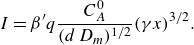 \begin{equation} I = \beta ' q \frac {C_A^0}{(d \, D_{{m}})^{1/2}}{(\gamma x)}^{3/2}. \end{equation}
The prefactor $\beta '$
in (4.20) is the sole fitting parameter and is expected to be the same for all experiments performed in the saddle-flow configuration. The pore-scale mixing theory agrees well with the data for the distance range considered and the Péclet numbers (figure 10
b). As a reference, we also plot the predictions of the dispersion model in figure 10(b). Although it matches the experimental curves at distances smaller than the pore size, i.e. for low velocities in the saddle flow, the dispersion model largely diverges from the data at larger distances for all Péclet numbers. In contrast, the mixing model captures the observed evolution of the reaction intensity with both distance (figure 10
b) and Péclet number (figure 8
b1). Note that, contrary to the co-flow configuration, there is no transition to the dispersive scaling at large distances. In saddle flows, the supply of reactants on both sides of the front increases linearly with distance (figure 2), allowing for a continuous supply of fresh reactants. Hence there is no limitation of reactant supply by dispersion, and the effect of pore-scale mixing persists over the whole range of experimental observations.
$\beta '$
in (4.20) is the sole fitting parameter and is expected to be the same for all experiments performed in the saddle-flow configuration. The pore-scale mixing theory agrees well with the data for the distance range considered and the Péclet numbers (figure 10
b). As a reference, we also plot the predictions of the dispersion model in figure 10(b). Although it matches the experimental curves at distances smaller than the pore size, i.e. for low velocities in the saddle flow, the dispersion model largely diverges from the data at larger distances for all Péclet numbers. In contrast, the mixing model captures the observed evolution of the reaction intensity with both distance (figure 10
b) and Péclet number (figure 8
b1). Note that, contrary to the co-flow configuration, there is no transition to the dispersive scaling at large distances. In saddle flows, the supply of reactants on both sides of the front increases linearly with distance (figure 2), allowing for a continuous supply of fresh reactants. Hence there is no limitation of reactant supply by dispersion, and the effect of pore-scale mixing persists over the whole range of experimental observations.
5. Conclusion
We investigated experimentally and theoretically the dynamics of a bimolecular reaction in steady mixing fronts in porous media. Two common flow configurations were considered, namely, a uniform flow and a converging flow. We first derived the effective reaction rates on the basis of the classical hydrodynamic dispersion model, which assumes well-mixed pore-scale conditions. We then experimentally measured the effective reaction rates in a cell filled with 3-D granular material. For this, we combined chemiluminescence and refractive-index matching, allowing us to precisely map the Darcy-scale reaction rates, integrated over the cell gap, across the mixing front.
Experimental reaction rates in the mixing zone show a significant departure from the predictions expected by modelling mixing with hydrodynamic dispersion. In co-flow, differences persist for approximately $20$
grain diameters, while in saddle flow, they persist throughout the front. Therefore, these findings highlight the role of incomplete mixing at the pore scale in reactive fronts. Building on the recent demonstration of the chaotic nature of mixing at the pore scale in 3-D porous media, we propose a new description of micro-scale reactive mixing dynamics to explain our Darcy-scale observations. This model leads to new scaling laws for effective reaction rates in porous media, as a function of both space and Péclet number.
$20$
grain diameters, while in saddle flow, they persist throughout the front. Therefore, these findings highlight the role of incomplete mixing at the pore scale in reactive fronts. Building on the recent demonstration of the chaotic nature of mixing at the pore scale in 3-D porous media, we propose a new description of micro-scale reactive mixing dynamics to explain our Darcy-scale observations. This model leads to new scaling laws for effective reaction rates in porous media, as a function of both space and Péclet number.
Although predictions accurately capture the general experimental trends, additional data are needed to uncover the details of micro-scale reactive mixing and its impact at the Darcy scale. Such data would require resolving both the pore-scale dynamics and the Darcy-scale effective reaction rates, a range of scales that is difficult to achieve experimentally with optical methods. Numerical simulations of large flow domains (Sole-Mari, Bolster & Fernàndez-Garcia Reference Sole-Mari, Bolster and Fernàndez-Garcia2022) or porous flow analogues (Heyman, Lester & Le Borgne Reference Heyman, Lester and Le Borgne2021) may be able to provide such data in the future.
Finally, our findings suggest that micro-scale mixing processes in porous media have an important effect on macroscopic reaction rates, an effect that persists for long time and distances along mixing fronts. The framework proposed to capture these processes, based on the physics of pore-scale flows (Lester et al. Reference Lester, Metcalfe and Trefry2013), opens new avenues for upscaling reactive transport at Darcy scale, beyond the hydrodynamic dispersion paradigm.
Acknowledgements.
Views and opinions expressed are those of the author(s) only, and do not necessarily reflect those of the European Union or the European Research Council Executive Agency. Neither the European Union nor the granting authority can be held responsible for them.
Funding.
Funded by the European Union (ERC, CHORUS, 101042466).
Declaration of interests.
The authors report no conflict of interest.
Data availability statement.
The data and codes to reproduce the findings of this study are openly available in Github at https://github.com/jorishey1234/reactivefronts or upon reasonable request to joris.heyman@univrennes.fr.
Appendix A. Theory of reactive mixing at finite Damköhler number
A.1. Reaction–diffusion front
Gálfi & Rácz (Reference Gálfi and Rácz1988) and Larralde et al. (Reference Larralde, Araujo, Havlin and Stanley1992) proposed an approximate solution to the equation of advection–diffusion–reaction in the case of one-dimensional fronts. The theory allows for the derivation of the asymptotic scaling with time and Damköhler number of the effective reaction front properties at the Darcy scale. Here, we recall the main steps of the derivation. We take dimensionless variables for space $y=\tilde {y}/L$
and time
$y=\tilde {y}/L$
and time $t=\tilde {t}/t_D$
, with
$t=\tilde {t}/t_D$
, with $L$
a length scale, and
$L$
a length scale, and $t_D=L^2/D_{{m}}$
the diffusion time, and dimensionless concentrations
$t_D=L^2/D_{{m}}$
the diffusion time, and dimensionless concentrations $C_i=\tilde {C_i}/C_A^0$
. The ratio of initial reactant concentrations is
$C_i=\tilde {C_i}/C_A^0$
. The ratio of initial reactant concentrations is $q=C_B^0/C_A^0$
. In our experiments,
$q=C_B^0/C_A^0$
. In our experiments, $q=2$
. The dimensionless reaction–diffusion equation reads
$q=2$
. The dimensionless reaction–diffusion equation reads
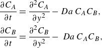 \begin{align} \frac {\partial {C}_A}{\partial {t}} &= \frac {\partial ^2 {C}_A}{\partial {y}^2}- Da \, {C}_A {C}_B, \notag \\ \frac {\partial {C}_B}{\partial {t}} &= \frac {\partial ^2 {C}_B}{\partial {y}^2}- \, Da \, {C}_A {C}_B, \end{align}
where $Da=t_D/t_r$
is the Damköhler number, and
$Da=t_D/t_r$
is the Damköhler number, and $t_r = 1/(k C_A^0)$
is the characteristic reaction time. It is easy to show that
$t_r = 1/(k C_A^0)$
is the characteristic reaction time. It is easy to show that $F=C_A- C_B$
is a conserved quantity obeying an advection–diffusion equation. For initially segregated reactants with initial conditions
$F=C_A- C_B$
is a conserved quantity obeying an advection–diffusion equation. For initially segregated reactants with initial conditions $F=1$
for
$F=1$
for $y\lt 0$
and
$y\lt 0$
and $F=-q$
for
$F=-q$
for $y\gt 0$
,
$y\gt 0$
, $F$
follows
$F$
follows
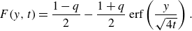 \begin{equation} F(y,t)= \frac {1-q}{2}-\frac {1+q}{2} \,\text{erf} \left ( \frac {y}{\sqrt {4t}} \right ). \end{equation}
The front position is located at $F=0$
, i.e. at
$F=0$
, i.e. at
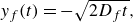 \begin{equation} y_f(t) = - \sqrt {2 D_f t}, \end{equation}
where the constant $D_f$
is a solution of
$D_f$
is a solution of
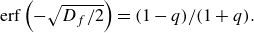 \begin{equation} \text{erf}\left ( -\sqrt {D_f/2} \right )=(1-q)/(1+q). \end{equation}
Note that if $q=1$
(equal reactant concentrations), then
$q=1$
(equal reactant concentrations), then $D_f=0$
and
$D_f=0$
and $y_f=0$
at all times. For the chemiluminescence reaction considered,
$y_f=0$
at all times. For the chemiluminescence reaction considered, $q=2$
and
$q=2$
and $D_f \approx 0.1855$
. Inserting (A2) into (A1), a nonlinear equation is obtained for
$D_f \approx 0.1855$
. Inserting (A2) into (A1), a nonlinear equation is obtained for $C_A$
:
$C_A$
:
 \begin{equation} \frac {\partial C_A}{\partial t} = \frac {\partial ^2 C_A}{\partial {y} ^2}+ \, Da \, C_A \left (F(y,t)-C_A \right ). \end{equation}
Equation (A5) can be approximated if the penetration of reactants is limited to a small region near $y=y_f$
, i.e. for intermediate Damköhler numbers (Gálfi & Rácz Reference Gálfi and Rácz1988; Larralde et al. Reference Larralde, Araujo, Havlin and Stanley1992). Neglecting the
$y=y_f$
, i.e. for intermediate Damköhler numbers (Gálfi & Rácz Reference Gálfi and Rácz1988; Larralde et al. Reference Larralde, Araujo, Havlin and Stanley1992). Neglecting the $C_A^2$
term and taking an expansion of the error function near the front position
$C_A^2$
term and taking an expansion of the error function near the front position $y_f$
, we get
$y_f$
, we get
 \begin{equation} \frac {\partial C_A}{\partial t} = \frac {\partial ^2 C_A}{\partial y ^2}- q'\, Da \, C_A \frac {y-y_f}{\sqrt { t}}, \end{equation}
with $q'=(1+q) \exp (-D_f/2) / (2\sqrt {\pi })$
(Gálfi & Rácz Reference Gálfi and Rácz1988). The solution to this equation can be found by recognising the Airy differential problem on the right-hand side of (A6), such that a solution for
$q'=(1+q) \exp (-D_f/2) / (2\sqrt {\pi })$
(Gálfi & Rácz Reference Gálfi and Rácz1988). The solution to this equation can be found by recognising the Airy differential problem on the right-hand side of (A6), such that a solution for $C_A$
is
$C_A$
is
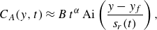 \begin{equation} C_A(y,t) \approx B \, t^{\alpha } \,\text{Ai}\left ( \frac { y-y_f}{{s}_r(t)} \right ), \end{equation}
where $\text{Ai}$
is the Airy function, and
$\text{Ai}$
is the Airy function, and ${s}_r(t)=(q' \, Da)^{-1/3} t^{1/6}$
is a dimensionless reactive width. The dimensional reactive width reads
${s}_r(t)=(q' \, Da)^{-1/3} t^{1/6}$
is a dimensionless reactive width. The dimensional reactive width reads
 \begin{equation} \tilde {s}_r(t)=L {s}_r= L (q' \, Da)^{-1/3} (D_{{m}} \tilde {t} /L^2 )^{1/6}. \end{equation}
Finding $\alpha$
and
$\alpha$
and $B$
is possible by equating the nonlinear term with the spatial derivative in (A5), giving
$B$
is possible by equating the nonlinear term with the spatial derivative in (A5), giving $\alpha =-1/3$
and
$\alpha =-1/3$
and $B \sim q'^{2/3} Da^{-1/3}$
.
$B \sim q'^{2/3} Da^{-1/3}$
.
The reaction rate is also the source term of (A6), such that
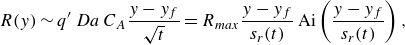 \begin{equation} R(y) \sim q' \, Da \, C_A \frac {y-y_f}{\sqrt { t}} = R_{{max}} \frac {y-y_f}{ {s}_r(t)} \,\text{Ai}\left ( \frac { y-y_f}{{s}_r(t)} \right ), \end{equation}
with the maximal reaction rate $R_{{max}}\sim q'^{4/3} \, Da^{1/3} \, t^{-2/3}$
. The dimensional max reaction rate is
$R_{{max}}\sim q'^{4/3} \, Da^{1/3} \, t^{-2/3}$
. The dimensional max reaction rate is
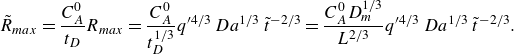 \begin{equation} \tilde {R}_{{max}} = \frac {C_A^0}{t_D} R_{{max}} = \frac {C_A^0}{t_D^{1/3}} q'^{4/3}\, Da^{1/3}\, \tilde {t}^{-2/3} = \frac {C_A^0 D_{{m}}^{1/3}}{L^{2/3}} q'^{4/3}\, Da^{1/3}\, \tilde {t}^{-2/3}. \end{equation}
The total reaction intensity is
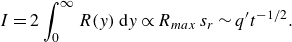 \begin{equation} I = 2\int _0^{\infty } R(y)\, \text{d}y \propto R_{{max}} \, s_r \sim q' t^{-1/2}. \end{equation}
Its dimensional equivalent is
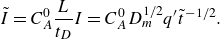 \begin{equation} \tilde {I} = C_A^0 \frac {L}{t_D} I = C_A^0 D_{{m}}^{1/2} q' \tilde {t}^{-1/2}. \end{equation}
Note that this result can also be recovered by considering the infinitely fast reaction case, where the intensity of reaction is exactly equal to the diffusive flux across the interface:
 \begin{equation} \tilde {I} \sim D_{{m}} \frac {\partial C_A}{\partial y} \sim D_{{m}} \frac {C_A^0}{\sqrt {D_{{m}} \tilde {t}}}, \end{equation}
which is equivalent to (A12). In fact, the finite and infinite Damköhler cases yield equal scaling for the total reaction intensity. The difference emerges in the existence of a finite reaction width and a maximum reaction rate.
A.2. Advection–diffusion–reaction front
In the case of an advection at constant velocity $U$
, the preceding results simply hold with
$U$
, the preceding results simply hold with $\tilde {x}=\tilde {t} U$
, or equivalently,
$\tilde {x}=\tilde {t} U$
, or equivalently, $t=x\, Pe$
. This implies that
$t=x\, Pe$
. This implies that
 \begin{align}&\,\, {s}_R \sim (q' \, Da)^{-1/3}\, Pe^{-1/6}\, {x}^{1/6}, \end{align}
 \begin{align}& R_{{max}} \sim q'^{4/3} \, Da^{1/3}\, Pe^{2/3}\, {x}^{-2/3} \end{align}
and
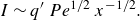 \begin{equation} I \sim q' \, Pe^{1/2} \, x^{-1/2}. \end{equation}
A.3. Advection–diffusion–reaction with compression
In the presence of a constant compression rate $\gamma =U/(2 L)$
, the conservative profile
$\gamma =U/(2 L)$
, the conservative profile $F$
reaches a steady state:
$F$
reaches a steady state:
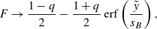 \begin{equation} F \to \frac {1-q}{2} -\frac {1+q}{2}\,\text{erf}\left (\frac {\tilde {y}}{s_B}\right ), \end{equation}
with the Batchelor scale $s_B=\sqrt {2 D_{{m}}/\gamma }$
(Villermaux Reference Villermaux2019). Since
$s_B=\sqrt {2 D_{{m}}/\gamma }$
(Villermaux Reference Villermaux2019). Since $Pe=L^2 \gamma / D_{{m}}$
, this is also
$Pe=L^2 \gamma / D_{{m}}$
, this is also
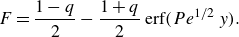 \begin{equation} F= \frac {1-q}{2} -\frac {1+q}{2} \,\text{erf}(Pe^{1/2}\, y). \end{equation}
The front location $F=0$
is now fixed to
$F=0$
is now fixed to $y_f$
, the solution of
$y_f$
, the solution of
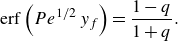 \begin{equation} \text{erf} \left ( Pe^{1/2}\, y_f \right ) =\frac {1-q}{1+q}. \end{equation}
The above derivations still hold, without the time dependence. The equation for $C_A$
reads
$C_A$
reads
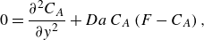 \begin{equation} 0 = \frac {\partial ^2 C_A}{\partial {y} ^2} + Da \, C_A\left (F-C_A\right ), \end{equation}
whose approximate solution is
 \begin{equation} C_A \sim B \,\text{Ai}\left ( \frac {y-y_f}{s_r}\right ), \end{equation}
with $s_r=(q' \, Da)^{-1/3}\,Pe^{-1/6}$
and
$s_r=(q' \, Da)^{-1/3}\,Pe^{-1/6}$
and $B\sim q'^{2/3}\, Da^{-1/3}\, Pe^{1/3}$
. As before,
$B\sim q'^{2/3}\, Da^{-1/3}\, Pe^{1/3}$
. As before, $B$
is determined by scaling the nonlinear term with the spatial derivative in (A20). Then the reaction rate is
$B$
is determined by scaling the nonlinear term with the spatial derivative in (A20). Then the reaction rate is
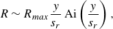 \begin{equation} R \sim R_{{max}} \frac {y}{s_r} \,\text{Ai}\left ( \frac {y}{s_r}\right ), \end{equation}
with
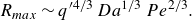 \begin{equation} R_{{max}} \sim q'^{4/3}\, Da^{1/3}\, Pe^{2/3}. \end{equation}
The total reaction intensity is
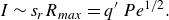 \begin{equation} I\sim s_r R_{{max}} = q' \, Pe^{1/2}. \end{equation}
In dimensional form, these read
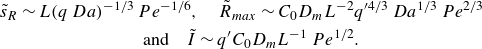 \begin{align} &\tilde {s}_R \sim L (q\, Da)^{-1/3}\,Pe^{-1/6},\quad \tilde {R}_{{max}} \sim C_0 D_{{m}} L^{-2} q'^{4/3}\, Da^{1/3}\, Pe^{2/3} \nonumber\\&\qquad\qquad\qquad\qquad\text{and} \quad \tilde {I} \sim q' C_0 D_{{m}} L^{-1}\, Pe^{1/2}. \end{align}
A.4. Numerical simulation of dispersion–reaction fronts
We validated the theoretical scaling of reactive fronts under dispersion in uniform flow (2.18)–(2.22) against numerical simulations of the full 2-D advection–dispersion–reaction problem (2.1). To numerically solve the equations, we use the OpenFOAM finite-volume software (https://openfoam.org). The domain is a 2-D rectangle; for co-flow, $x\in [0,150]$
mm with 300 grid cells,
$x\in [0,150]$
mm with 300 grid cells, $y\in [-25,25]$
mm with 400 cells, and for saddle flow,
$y\in [-25,25]$
mm with 400 cells, and for saddle flow, $x\in [-150,150]$
mm with 600 cells,
$x\in [-150,150]$
mm with 600 cells, $y\in [-25,25]$
mm with 400 cells. We fixed
$y\in [-25,25]$
mm with 400 cells. We fixed $D_{{m}}=5\times 10^{-10}$ $\mathrm{m^2\ s^{-1}}$
, and varied
$\mathrm{m^2\ s^{-1}}$
, and varied $U$
or
$U$
or $\gamma$
. We used an isotropic dispersivity tensor with
$\gamma$
. We used an isotropic dispersivity tensor with $\alpha _T=\alpha _L=0.06d$
m, where
$\alpha _T=\alpha _L=0.06d$
m, where $d$
is the grain size (2 mm). The reaction rate constant is fixed at
$d$
is the grain size (2 mm). The reaction rate constant is fixed at $k = 0.08$ $\mathrm{mM^{-1}\ s^{-1}}$
. We used a kinetic rate that is 10 times smaller than the experimental value such that the width of the simulated fronts is approximately the same as the one observed experimentally. This net difference highlights the fact that the porous medium efficiently spreads the reactants but without completely mixing them (retarding reaction). To match the observed reactive width with a hydrodynamic dispersion model, it is necessary to slow down the reaction kinetics so that the reactive width approaches the dispersive width. The solute concentration at the inlet boundary of the co-flow (at
$\mathrm{mM^{-1}\ s^{-1}}$
. We used a kinetic rate that is 10 times smaller than the experimental value such that the width of the simulated fronts is approximately the same as the one observed experimentally. This net difference highlights the fact that the porous medium efficiently spreads the reactants but without completely mixing them (retarding reaction). To match the observed reactive width with a hydrodynamic dispersion model, it is necessary to slow down the reaction kinetics so that the reactive width approaches the dispersive width. The solute concentration at the inlet boundary of the co-flow (at $x = 0$
) was
$x = 0$
) was $(C_A,C_B) = (1,0)$
mM for
$(C_A,C_B) = (1,0)$
mM for $y\gt 0$
, and
$y\gt 0$
, and $(C_A,C_B) = (0,1)$
mM for
$(C_A,C_B) = (0,1)$
mM for $y\lt 0$
. The inlet boundary condition of the saddle flow was
$y\lt 0$
. The inlet boundary condition of the saddle flow was $(C_A,C_B) = (1,0)$
mM at
$(C_A,C_B) = (1,0)$
mM at $y=50$
, and
$y=50$
, and $(C_A,C_B) = (0,1)$
mM at
$(C_A,C_B) = (0,1)$
mM at $y=-50$
mm. For the outlet boundaries (
$y=-50$
mm. For the outlet boundaries ( $x=150$
mm for co-flow, and
$x=150$
mm for co-flow, and $y=\pm 50$
mm for saddle flow), we imposed a zero gradient for all species. We used the Euler method as a temporal discretisation scheme, and a linear interpolation scheme for interpolating face-centred values from cell-centred values. We varied the velocity
$y=\pm 50$
mm for saddle flow), we imposed a zero gradient for all species. We used the Euler method as a temporal discretisation scheme, and a linear interpolation scheme for interpolating face-centred values from cell-centred values. We varied the velocity $U$
(co-flow) and compression rate
$U$
(co-flow) and compression rate $\gamma$
(saddle flow) in the same range as in the experiments. The characteristic length scale to define the Péclet number in the co-flow is the diameter of the grain,
$\gamma$
(saddle flow) in the same range as in the experiments. The characteristic length scale to define the Péclet number in the co-flow is the diameter of the grain, $L = 2$
mm. In saddle flow, the characteristic velocity is
$L = 2$
mm. In saddle flow, the characteristic velocity is $U=\gamma L$
, with the length
$U=\gamma L$
, with the length $L=100$
mm corresponding to our experimental set-up (see § 3.1.2). Such definitions resulted in simulations with
$L=100$
mm corresponding to our experimental set-up (see § 3.1.2). Such definitions resulted in simulations with $Pe$
ranging from 179 to 3575 for co-flow, and from 434 to 8678 for saddle flow. The spatial behaviour of the reactive fronts in the presence of dispersion is plotted in figure 11.
$Pe$
ranging from 179 to 3575 for co-flow, and from 434 to 8678 for saddle flow. The spatial behaviour of the reactive fronts in the presence of dispersion is plotted in figure 11.
Normalised reaction rate fields at $Pe= 799$
, 1690 and 3575 for co-flow, and
$Pe= 799$
, 1690 and 3575 for co-flow, and $Pe= 1941$
, 4104 and 8678 for saddle flow (lowest at the top row, highest at the bottom row) from simulations for porous media. The reaction rate is normalised by the maximum reaction rate at the highest
$Pe= 1941$
, 4104 and 8678 for saddle flow (lowest at the top row, highest at the bottom row) from simulations for porous media. The reaction rate is normalised by the maximum reaction rate at the highest $Pe$
for each configuration. For co-flow, the left-hand edge corresponds to the start of mixing, and for saddle flow, the left-hand edge corresponds to the stagnation point. The white dashed lines in the lowest
$Pe$
for each configuration. For co-flow, the left-hand edge corresponds to the start of mixing, and for saddle flow, the left-hand edge corresponds to the stagnation point. The white dashed lines in the lowest $Pe$
in experimental images show the streamlines.
$Pe$
in experimental images show the streamlines.
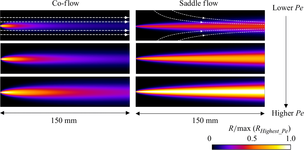
A.5. Simulation results
The dependences of the maximum reaction rate $R_{{max}}$
, total reaction intensity
$R_{{max}}$
, total reaction intensity $I$
and reaction width
$I$
and reaction width $s_R$
with position
$s_R$
with position $x$
along the front in co-flow and saddle flows are plotted in figures 12 and 13 respectively, as well as the theoretical predictions (2.18)–(2.22). The predictions show very good agreement with the simulations. Next, the front properties are plotted against
$x$
along the front in co-flow and saddle flows are plotted in figures 12 and 13 respectively, as well as the theoretical predictions (2.18)–(2.22). The predictions show very good agreement with the simulations. Next, the front properties are plotted against $Pe$
at a given location
$Pe$
at a given location $x$
in figures 14 and 15 for the co-flow and saddle flows, respectively. In co-flow, the theoretical scaling laws compare well with simulations. On the other hand, in saddle flow, the scaling laws of the mixing-limited regime are verified only for low
$x$
in figures 14 and 15 for the co-flow and saddle flows, respectively. In co-flow, the theoretical scaling laws compare well with simulations. On the other hand, in saddle flow, the scaling laws of the mixing-limited regime are verified only for low $Pe$
. This is because the longitudinal derivatives that were dropped in (2.12) (
$Pe$
. This is because the longitudinal derivatives that were dropped in (2.12) ( $\gamma x\,\partial C_A/\partial x$
and
$\gamma x\,\partial C_A/\partial x$
and $\alpha _L \gamma\, |y|\,\partial ^2 C_A/\partial x^2$
) become large compared to
$\alpha _L \gamma\, |y|\,\partial ^2 C_A/\partial x^2$
) become large compared to $kC_AC_B$
, and the approximation becomes not valid at high
$kC_AC_B$
, and the approximation becomes not valid at high $Pe$
. Thus the approximation is valid for low to moderate
$Pe$
. Thus the approximation is valid for low to moderate $Pe$
. To compare with the experiments, the scaling exponents were derived by fitting the simulation results.
$Pe$
. To compare with the experiments, the scaling exponents were derived by fitting the simulation results.
Scaling of reactive front properties with distance to injection in co-flow with hydrodynamic dispersion obtained by numerical simulations: (a) width of the reaction front, (b) maximum reaction rate, and (c) reaction intensity. Black dashed lines stand for the theoretical prediction (2.18) and (2.19).

Scaling of reactive front properties with distance to injection in saddle-flow with hydrodynamic dispersion obtained by numerical simulations: (a) width of the reaction front, (b) maximum reaction rate, and (c) reaction intensity. Black dashed lines stand for the theoretical prediction in the kinetic-limited regime (2.21).
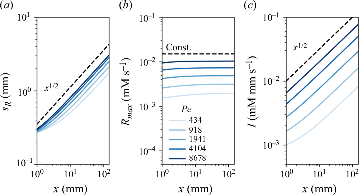
Simulated reactive front over $Pe$
at 150 mm in co-flow under hydrodynamic dispersion: (a) width of the reaction, (b) maximum reaction rate, and (c) reaction intensity. Black dashed lines are the hydrodynamic dispersion predictions for the mixing-limited regime at fixed time (2.19).
$Pe$
at 150 mm in co-flow under hydrodynamic dispersion: (a) width of the reaction, (b) maximum reaction rate, and (c) reaction intensity. Black dashed lines are the hydrodynamic dispersion predictions for the mixing-limited regime at fixed time (2.19).

Simulated reactive front over $Pe$
at 150 mm in saddle flow under hydrodynamic dispersion: (a) width of the reaction, (b) maximum reaction rate, and (c) reaction intensity. The green dashed lines are hydrodynamic dispersion predictions of reaction limited regime (2.21), whereas the black dashed lines are those of mixing-limited regime (2.22). The blue dashed lines show fitted lines with fitted exponent.
$Pe$
at 150 mm in saddle flow under hydrodynamic dispersion: (a) width of the reaction, (b) maximum reaction rate, and (c) reaction intensity. The green dashed lines are hydrodynamic dispersion predictions of reaction limited regime (2.21), whereas the black dashed lines are those of mixing-limited regime (2.22). The blue dashed lines show fitted lines with fitted exponent.
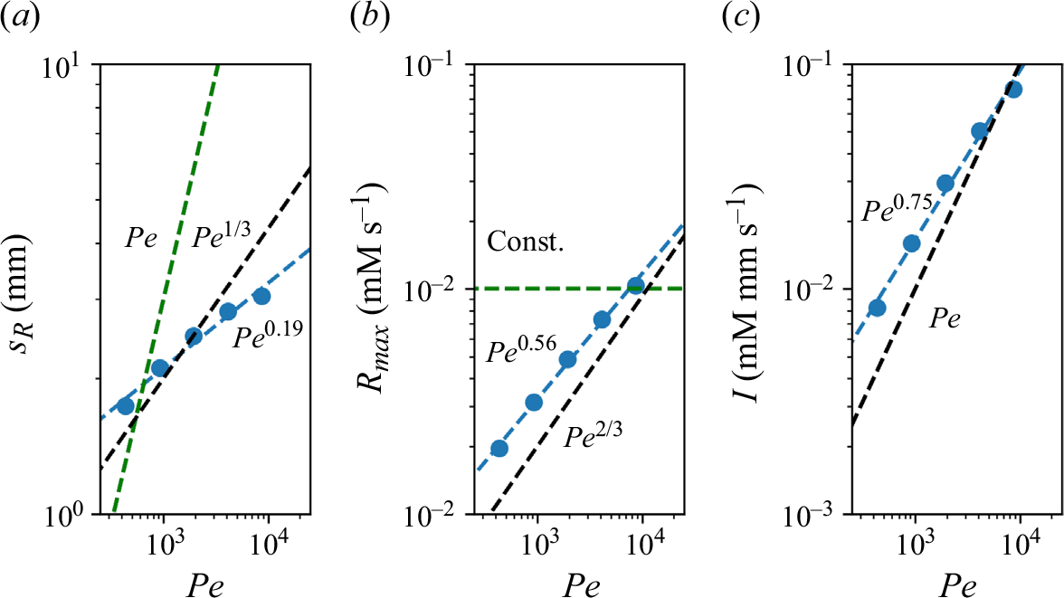


 Open access