2.1. The adjoint or Lagrange multiplier method

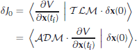
Our goal is to find sensitivities, i.e. partial derivatives of a scalar-valued objective or cost function J₀[x] with respect to control variables u. The dependency ofJ ₀ on u is usually indirect, i.e. through the dependency of elements of state variables x of a model on u. For simplicity, we focus on the case where u is the model’s initial state x(t ₀ = 0). Following the notation of Reference WunschWunsch (2006), the time-dependent modelL has the general form

(1)

and is integrated from timet ₀ = 0 tot =t _f. (To simplify notation, we can formally extend the model state space x to include model prognostic variables as well as model parameters and boundary conditions.)

As an example, let the objective function consist of the time-mean volume over the lastn+1 time-stepst _f −n,. . . ,t _f − 1,t _f of the ice sheet, expressed as the spatial, area-weighted sumV[x(t)] =Σ _i,j H(i,j,t) dA(i,j) over the thickness field H(t) at timet, which is an element of the model prognostic state space x(t). We therefore have

(2)

The Lagrange multiplier method consists of rewriting the problem of finding derivatives ofJ ₀, subject to the constraint of fulfilling Equation (1), into an extended and unconstrained problem:

(3)

For each element of the model state x(t) at timet, we have introduced a corresponding Lagrange multiplier μ(t).

The set of normal equations is obtained by requiring the partial derivatives of Equation (3) with respect to each variable for times t >t ₀ to vanish independently (e.g. Reference WunschWunsch, 2006):

(4a)

(4b)

(4c)

(4d)

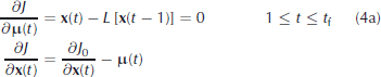
Equation (4a) simply recovers the model equations. The Lagrange multipliers μ(t) are found through successive evaluation of the normal equations backwards in time.

Starting att =t _f we find (via Equation (4c) and using example cost Equation (2)),

n + 1 time-steps earlier att =t _f − n. Using the results of μ(t _f),. . . ,μ(t _f − n + 1), we obtain (using Equation (4b)):

(5)

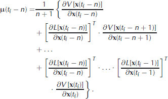
Finally, Equation (4d) provides the expression for the full gradient sought at timet ₀ = 0.

We make the following interpretation. The Lagrange multiplier μ(t) provides the complete sensitivity ofJ ₀ at timet by accumulating all partial derivatives ofJ ₀ with respect to x from each time-stept _f ,t _f −1,. . . ,t. Those partial derivatives taken at later timest +1,. . . ,t _f are propagated to timet via the ADM, which is the transpose

of the model Jacobian or tangent linear model (TLM)

with contributions from different times linearly superimposed. Further simplifying the example objective function (2) to the special case where instead of the time-mean only the volume at the last time-stept _f is chosen, i.e.n = 0, Equation (5) simplifies in that all terms vanish except for that containing

2.2. The tangent linear and adjoint models

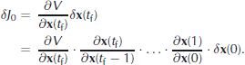
All relevant aspects of the LMM have now been derived, but we wish to make plain the duality between the TLM and the ADM. We restate our problem in a slightly different but equivalent framework which provides a natural basis for introducing the concept of AD. The non-linear model (NLM)L of Equation (1) may be viewed as a mapping of the state space (again incorporating all parameters and initial and boundary conditions into an extended state space) from timet = 0 tot =t _f. The cost functionJ ₀ (Equation (2)) is then a composite mapping from the state space att ₀ = 0 tot =t _f, and from there to the real numbers. To simplify notation, let y = x(t _f) and consider the special casen = 0, i.e.J ₀ =V[x(t _f)] =V[y]. Then,

(6)

The composite nature of the mapping ofJ ₀ is readily apparent:

(7)

A perturbation of the initial state x(0) is linked to a perturbation ofJ ₀ by applying the chain rule to Equation (7):

(8)

Recognizing thatδJ₀ is simply the scalar product of andδy, we can use the formal definition of an adjoint operator (x | Ay)= (A^Tx|y) to rewrite this equation:

(9)

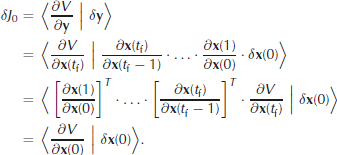
Alternatively, by denoting the tangent linear and adjoint matrices asTLM andADM, respectively, we have:

(10)

Equations (5), (9) and (10) highlight various features:

1. the equivalence between Lagrange multipliers and the adjoint operator;

2. the fact that the TLM runs forward in time, propagating the effect of a perturbationδx(0) to all model outputs, while the ADM runs backward, accumulating sensitivities ofδJ₀ to all model inputs; and

3. the advantage of the ADM, which provides the full gradient of a model-constrained objective function∂V/∂x(0) over the TLM which only provides the projection of∂V/∂y onto the perturbed vectorδy from initial perturbationδx(0).

2.3. Derivative code generation via automatic differentiation

Although we have demonstrated the power of the adjoint method, we have not yet discussed how to obtain it. In general, the complexity and effort involved in developing an adjoint model matches that in its parent NLM development and frequently prohibits adjoint model applications. An alternative to hand-coding the adjoint (i.e. coding the discretized adjoint equations) and a major step forward is the use of AD compared to derivative (e.g. ADM or TLM) code generation (Reference Griewank and WaltherGriewank and Walther, 2008). The advent of AD source-to-source transformation tools such as the commercial tool ‘Transformation of Algorithms in Fortran’ (TAF) (Reference Giering, Kaminski and SlawigGiering and others, 2005) or the open-source tool OpenAD (Reference UtkeUtke and others, 2008) has enabled the development of exact adjoint models from complex, nonlinear forward models. In the oceanographic context, there is now a decade of experience in applying this method to a state-of-the-art ocean general circulation model (e.g. Reference Marotzke, Giering, Zhang, Stammer, Hill and LeeMarotzke and others, 1999; Reference Galanti, Tziperman, Harrison, Rosati, Giering and SirkesGalanti and others, 2002; Reference Heimbach, Hill, Giering, Dongarra, Sloot and TanHeimbach and others, 2002; Reference StammerStammer and others, 2003; Reference HeimbachHeimbach, 2008) which encourages us to apply such tools to state-of-the-art ice-sheet models.

The composite nature of the mappingJ ₀ is that of a large number of elementary operations; Equation (6) reflects this at the time-stepping level. Carrying the concept of composition to its extreme, ultimately each line of code can be viewed as an elementary operation. At the elementary level, the AD tool knows the complete set of derivatives (i.e. the elementary Jacobians)√ for each intrinsic arithmetic function (+, –, *,/,√., sin(.), etc.), as well as logical/conditional instructions.

Here, we demonstrate how the AD tool generates line-byline elementary Jacobians (TLM code) and their transpose (ADM code). The full model Jacobian is recovered by composition of each elementary Jacobian according to the chain and product rule. A very simple example is given in Figure 1, demonstrating the relationship between the NLM, TLM and ADM. The full derivative is readily calculated (line TLM), and the adjoint model easily derived by taking the transposes of dJ₀ and dL. It is readily apparent that while the TLM only provides a projection of the gradient onto the directional perturbation vectorδx, the ADM provides the full gradient vector.

Fig. 1. Example of the relationship between the NLM, the TLM and the ADM. The general formalism is summarized in the upper table for a squared-valued cost functionJ ₀ =|y| ². The lower table provides a written example for a simple 2-D vector modelL, one time-step of which consists of a rotation and stretching followed by evaluation of the squared costJ ₀.

In the context of a more complex model, we chose as an example the advection problem arising from solving the continuity equation for the ice-sheet volume, expressed in terms of ice-sheet elevationH. The velocityU _b at which basal sliding-related advection takes place is inferred from a Weertman-type sliding law. Part of the time-stepping loop at timem might look like the chart in Figure 2.

Fig. 2. Upper box shows a simplified time-stepping loop of the nonlinear forward model; lower box shows the time-reversed adjoint time-stepping. Note the reversal of the order of sub-routine calls.

At the elementary level, the full derivative of the code line forU _b can be written (dropping superscriptm):

(11)

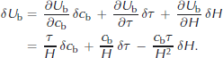
This can be rearranged in matrix form (Reference Giering and KaminskiGiering and Kaminski, 1998):

(12)

where the variablesδc _b,δτ,δH andδU _b are perturbations, i.e. elements of the TLM state space. Expressing the model in such a manner enables straightforward access to the transpose

(13)

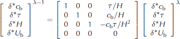
where the variablesδ∗c _b,δ∗τ,δ∗H and δ∗U _b are now sensitivities, i.e. elements of the adjoint model state space.

(Strictly, adjoint variables are co-vectors and are elements of the dual or co-tangent space to the tangent space of the model.) From Equation (13), we can readily calculate the following lines which represent the adjoint code:

(14)

The result can be interpreted in the following way.

1. From Equation (11) we infer how perturbations to the inputs affect the outputδU _b,whereas Equation (14) shows how the output sensitivityδ∗U _b has been influenced by each input sensitivity.

2. The aspect oftangent linear (and adjoint) is clear: knowledge of thecurrent state at timem of τ^m,H^m is necessary to evaluate either Equation (11) or Equation (14).

3. The TLM is evaluated in the same order as the non-linear parent modelL and evaluating both can be combined. The ADM is evaluated in reverse order, and making the required state variables accessible becomes a major problem in evaluating the adjoint model exactly.

Requiring the model state in reverse order is at the heart of the technical difficulties and one of the main hurdles in generating efficient and exact adjoint code for large-scale transient non-linear applications.

For the present study we have chosen the AD tool TAF. It solves the problem of requiring model state variables in reverse temporal order through a hierarchical ‘checkpointing’ and targeted ‘taping’ algorithm which provides a computationally efficient mix between saving and recomputing required variables. To achieve this, the user has to guide TAF through insertion of directives into the parent model to trigger storing of specific variables. A description is beyond the scope of this paper. Further details of the oceanographic context, as well as other topics (e.g. treatment of conditional (IF-) statements, (massive) parallel adjoint-code generation in the context of domain decomposition and treatment of implicit elliptic solvers) are given in Reference Heimbach, Hill and GieringHeimbach and others (2005).

As a final note of caution, because of thetangent linearity of the adjoint sensitivity, a limitation is that sensitivities are valid with respect to the reference model state for which they are computed. For purely linear problems they are independent of the reference state, but with increasing nonlinearity. Knowledge of the forward state becomes essential when interpreting such sensitivities; re-running the adjoint for different reference states may prove necessary. The implications are readily apparent from the example of a quadratic cost function provided in Figure 1. Nevertheless, since the same considerations apply to forward perturbation or TLM simulations, this does not constitute a disadvantage of the adjoint compared with forward methods.

2.4. Choice of control variables

Successful modeling requires relevant internal physics as well as appropriate representation of surface and basal boundary conditions. It is often the prescription of these which leads to significant differences in simulations.

At the surface of the ice sheet, interaction with the atmosphere is achieved through the prescription of meteorological and climatic inputs, consisting of surface mass-balance (accumulation minus ablation), precipitation, surface air temperature and refreezing and meltwater runoff parameterization (from positive degree-day method). Boundary conditions at the base of the ice sheet must account for interaction with the bedrock and the ocean, including basal sliding parameter, basal shear stress, basal melt/freeze rate, bed topography and geothermal heat flux. Finally, initial conditions are required for an ice sheet whose full 3-D state is usually poorly known and difficult to observe. The adjoint model provides sensitivities to each of these processes.

Boundary conditions are often heavily parameterized, and the sensitivity of the solution to the parameter choice can be substantial. Ultimately, all model ingredients that have associated uncertainties are relevant control variables.

Even quantities which are supposedly well determined, such as the precipitation products from the US National Centers for Environmental Prediction/US National Center for Atmospheric Research (NCEP/NCAR) (Reference KalnayKalnay and others, 1996) or the European Centre for Medium-Range Weather Forecasts (ECMWF) ERA-40 (Reference UppalaUppala and others, 2005) so-called ‘re-analyses’, have major uncertainties or biases, as discussed by Reference Bèranger, Barnier, Gulev and CrèponBèranger and others (2006). Their primary goal is to provide the best initial conditions for a subsequent forecast, but no requirements are imposed to preserve longterm global budgets. Furthermore, there is limited data coverage in polar regions, and they may be poorly constrained there. The finding by Reference Wingham, Shepherd, Muir and MarshallWingham and others (2006) that these fields ‘are not able to characterize the contemporary snowfall fluctuation with useful accuracy’ is therefore unsurprising.

3.1. Sensitivity to model parameters: the case of basal sliding and basal melt rate

Boundary conditions at the base of the ice sheet have an important, yet poorly understood, control on the evolution of the ice sheet. It is clear that the underlying model cannot simulate fast, realistic ice-stream flows, both because of the grid resolution and because of the use of the SIA. Nevertheless, even for long-term integrations for which this model seems more appropriate, the effect is relevant as it may provide a crucial mechanism for millennial-scale ice-sheet disintegration.

We investigate the effect of the sliding law with a Weertman-type parameterization ofU _b, which is a function of the (uncertain) sliding coefficientc _b (Reference GreveGreve, 1997, equation 5). The reference value used in the model is a spatially uniformc _b = 11.2ma− ¹ Pa− ¹. We makec _b a spatially dependent control variable, i.e.c _b =c _b(i,j). To put these sensitivities into context, we also derive sensitivities to basal melt rateq _bm. Equation (4.143) of Reference GreveGreve (1997) shows that this quantity is dependent on several factors. It is a function of vertical ice and lithosphere temperature gradients (with corresponding conductivity coefficients), as well as horizontal gradients of sliding velocityU _b times the vertical shear stress components in each direction. We only consider their cumulative effect here and represent the sensitivity by a spatially varying control variablea ₀ =q _bm L, basal melt rate times latent heatL = 3.35× 10⁵ J kg− ^₁ .

Figure 5a and b depict∂V/∂c _b and∂V/∂a ₀, respectively, the sensitivities of total ice volume to basal sliding and basal melt rates. The main features of sensitivity patterns can be summarized as follows.

Fig. 5. Adjoint sensitivity maps related to (a) basal sliding and (b) basal melt rate. A unit perturbationδc _b toc _b location (i,j) will change the cost functionV by the amountδV = (∂V/∂c _b)δc _b. To infer useful quantities forδV, we consider physically reasonable perturbations ofδc _b (e.g. representing typical standard deviations at this location, measurement uncertainties or model uncertainties). Qualitatively, melt-rate sensitivities (b) are fairly uniform where they do not vanish, whereas sliding sensitivities (a) exhibit significant regional variations.

1. The geographical variation of the sensitivities is readily apparent. Patterns of significant sensitivities are broadly similar. They are very small in the ice-sheet interior, but differ in detail where sensitivities are larger. Patterns of significanta ₀ sensitivities coincide with bottom-ice temperatures near the melting point and essentially vanish where temperatures fall below∼–3◦C. Largestc _b sensitivities are more concentrated near the margins of the ice sheet.

2. As expected, bothc _b anda ₀ sensitivities are mostly negative, i.e. increasing the basal sliding coefficient or the basal melt rate in most locations will reduce the total ice volume.

3. In contrast to the fairly uniform basal melt-rate sensitivities, those for basal sliding show conspicuous positive regions (region 2 in Fig. 3 and Table 1), implying that increasing the basal sliding coefficient increases the ice volume.

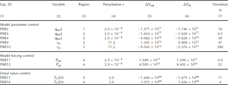
Table 1. Ice-volume changes inferred from adjoint sensitivities (column 5) and corresponding finite-difference perturbations (column 6) for various control variables (column 2) and perturbation regions (column 3). Perturbations 𝜖 are chosen to be 100% of base values (column 4) or assumed uncertainties (the former choice usually has a fairly large value compared to the latter). Reference total ice volume is V _ref = 3.248 × 10¹⁵ m³. The reasons for such large deviations are large perturbation values 𝜖 compared to mean; associated gradients are small and therefore noisy; or the presence of significant non-linearities, for which either the magnitude of 𝜖 or integration period (or both) are beyond the validity range of the assumption of linearity

3.2. Testing the adjoint sensitivities

Before proceeding, we make an important step in testing whether the computed adjoint sensitivities are reliable. We do so by performing a series of finite-perturbation simulations which we compare to adjoint-based perturbations. Table 1 summarizes the results. In particular, columns 5 and 6 represent values of total ice volume perturbations, which are computed as follows (e.g. fora ₀ as control):

Column 5: The value ΔV _adj at position (i,j) inferred from the adjoint sensitivity field∂V/∂a ^₀ (i,j) is obtained by integrating the sensitivities multiplied by a typical perturbationδ _a0 =є (column 4) over the region of interest (column 3) that is being perturbed, i.e.

(15)

Column 6: The value ΔV _fd is inferred by applying a uniform perturbationδ _a0 =є toa ₀ over the identical region (column 3) and performing a forward model simulation to compute the modifiedV(a ₀ +δ _a0). We therefore have:

(16)

We performed perturbation comparisons ofq _bm in four different regions (Table 1, experiments PAR2–PAR4). Given the localized nature of the perturbations, the smallness ofє (in most cases) and the shortness of the integration, the perturbed total ice volume remains comparatively small. Ice-volume changes computed from adjoint sensitivities deviate from finite-difference perturbations by 10%, 0.5% and 30% for regions 1–3 (cf.Fig. 1 and Table 1), respectively. The large deviation for PAR4 is associated with comparatively small perturbed values ofV (a factor of two smaller than for PAR2 and PAR3), indicating that the adjoint and finite-difference values are likely noisy in these cases. In contrast, for larger perturbedV there is good agreement between adjoint-derived and finite-difference perturbations (PAR2 and PAR3).

We have ascertained the validity of the gradient via finite-difference perturbations. Table 1 confirms both the positive gradient in region 2 (PAR9) and the negative gradient in nearby region 3 (PAR10). The changes in ice thicknessH _c incurred by the perturbation are plotted in Figure 6. Thec _b perturbations over region 2 lead to a dipole-like response inH _c (Fig. 6a), i.e. a decrease to the east of the perturbation and an increase over (and to the west of) the perturbation. The western thickness increase dominates the eastern decrease, leading to an overall positive ΔV as predicted by the adjoint. Region 3 just west of region 2 has a negative sensitivity and a mostly negative response pattern inH _c (Fig. 6b), again consistent with the adjoint inference.

Fig. 6. Response of ice-sheet elevation to perturbation in sliding coefficientc _b (Table 1, PAR9, PAR10). The differences between perturbed and unperturbed ice thicknesses (m) are depicted. The applied perturbation was fairly large (δc _b = 11.2ma− ^₁ Pa− ¹, which is 100% of the mean value). The aim is twofold: (1) to ascertain the sign and magnitude of the adjoint sensitivities and (2) to investigate the structure of the response to the perturbations and its physical causes. An upstream/downstream dipole pattern is apparent for the region 2 perturbation, with a dominating increase downstream of the perturbation. The region 3 perturbation (b) results mainly in a decrease in ice thickness.

Table 1. Ice-volume changes inferred from adjoint sensitivities (column 5) and corresponding finite-difference perturbations (column 6) for various control variables (column 2) and perturbation regions (column 3). Perturbationsє are chosen to be 100% of base values (column 4) or assumed uncertainties (the former choice usually has a fairly large value compared to the latter). Reference total ice volume isV _ref = 3.248× 10 ^₁₅ m³. The reasons for such large deviations are large perturbation valuesє compared to mean; associated gradients are small and therefore noisy; or the presence of significant non-linearities, for which either the magnitude ofє or integration period (or both) are beyond the validity range of the assumption of linearity

By increasing the sliding coefficient in region 3, it appears that while the ice thickness decreases upstream of the test region (relative to the flow direction), the rate of ice melt of the displaced ice just downstream of the perturbation is lower than for the unperturbed run. This may be due to ice emanating from further inland being further away from melting, thus temporarily reducing basal melt compared to the equilibrium case. The reduction of melt of the displaced ice therefore leads to overall increased ice volumes and the observed positive sensitivities.

3.3. Sensitivity to model forcing: the case of precipitation

A second important class of control variables is model forcings. The same adjoint calculation that provided the parameter sensitivity fields also furnishes sensitivities to various forcings, one of which we investigate in some detail (Fig. 7).

Fig. 7. Adjoint sensitivity maps of ice volume to precipitation for mean January (a) and July (b) conditions (10− ¹⁸ m³ (ms− ¹)− ¹). The interpretation is similar to that of Figure 5. Interior ice-sheet sensitivities are equal for summer and winter months, but values near the margins deviate strongly. An interpretation in terms of the seasonal snow-to-rain conversion function is given in the text.

The model uses an annual mean precipitation field as input. This field is first modified to account for elevation desertification with a threshold ice thickness of 2000 m. The resulting field is used to compute a mean annual snowfall, taking into account an annual cycle in surface air temperature. Accordingly, the snowfall for monthi is computed from the given annual mean precipitation, precip, and monthly mean surface air temperature fieldT _air(i) as

(17)

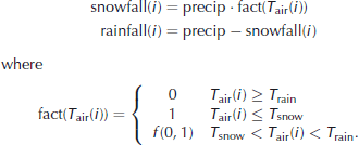
Here,T _rain= 7◦C andT _snow =−10◦C are threshold temperatures for precipitation which is equivalent to 100% rain and snow, respectively, andf (0, 1) is a function between 0 and 1. From this we can interpret the qualitative structure of the main differences between the adjoint sensitivity maps of January vs July precipitation (Fig. 7). We do so with the help of the adjoint statement of Equation (17), which we derive in the same way as for the adjoint code (Equation (14)):

(18)

In certain regions, and for months where fact(T _air(i)) = 1, January and July sensitivities coincide. In regions where the annual cycle in temperature exceeds the snow or even the rain threshold, the difference in sensitivities is greater. These regions are concentrated at low altitudes and near the coast. As a consequence, the ice volume sensitivities exhibit a seasonal dependence on precipitation induced by air temperature, and the equilibrium line is clearly visible. Sensitivities at the margins are significantly enhanced (large snow accumulation) during winter. During summer, however, they are strongly reduced if not reversed in sign due to melting.

Note that this example demonstrates that conditional statements (IF-statements) as represented by the function fact(T _air(i)) can be readily dealt with in the context of AD and adjoint code generation. They are best viewed as implementations of piecewise differentiable expressions. In fact, exact adjoint code relies on the availability of the exact branch of a condition when evaluating the adjoint.

3.4. Sensitivity to initial state

A third class of control variables concerns the initial conditions of the model. The main quantity of interest here is the 3-D ice temperature distribution. Its uncertainties are considerable: observations of the interior of the ice sheets, or even near the base, are almost entirely lacking. Assessing sensitivities of ice volume to changes in ice temperature anywhere in the ice sheet is therefore of considerable significance. In data assimilation, where initial conditions are sought from the model run to produce a best fit to observations (state estimation mode) or to produce an ‘optimal forecast’ (forecast mode), the initial condition control problem is essential. We therefore include a a brief discussion here.

Figure 8 depicts a sensitivity map at a randomly chosen vertical level of the ice sheet (note that because of the use of rescaled vertical coordinates, i.e. scaled thickness from 0 to 1, the ordinate does not reflect thickness itself but a level index). A complementary view is obtained by considering zonal or meridional cross-sections. Here we choose a north–south section ati = 32 (Fig. 9). Considerable regional variations are evident (both positive and negative areas exist), as are dependencies with respect to vertical position. Sensitivities are much larger near the base where temperatures are closer to the melting point, and are mostly negative (i.e. increasing the temperature will decrease the ice volume). Towards the surface the ice sheet seems insulated against significant ice-sheet volume sensitivities. As was the case for basal sliding, the temperature sensitivity maps contain evidence of the main drainage systems of the ice sheet, albeit coarsely represented at this resolution.

Fig. 8. Adjoint sensitivity of ice volume to ice temperature variations; vertical levelk = 20 (of 80, counted from ice-sheet base) (10− ⁶ m³ ◦C− ¹). Significant spatial variations are apparent, with conspicuous regions of positive sensitivities. A hint of drainage basins near the coast is evident. Maps similar to this would be used in data assimilation to infer model initial condition changes that lead to an improved model simulation vs observation misfit.

Fig. 9. Meridional section ati = 32 vs vertical level of adjoint ice temperature sensitivities across the ice sheet (10− ⁷ m³ ◦C− ¹). The plot complements Figure 8 in resolving the dependency of ice temperature sensitivities. Main features are insulation of sensitivities toward the ice sheet’s upper boundary; dominance of negative sensitivities, increasing in magnitude towards the ice-sheet base; and confirmation of the positive sensitivity band near, but not immediately adjacent to, the ice-sheet base.

Of particular interest is a significant band of positive sensitivities extending mostly in the north–south direction in the southwest sector of the ice sheet. This band is near the coast yet separated from it by a band of negative sensitivities. They seem to coincide with regions of positive sensitivities to changes in the basal sliding coefficientc ^_b (Fig. 5) which were attributed to the interaction between enhanced sliding and coastal ice melt rates. These patterns show that warming the ice will not necessarily have the uniform consequence of shrinking the ice sheet. They are unexpected, but confirmed by finite-difference perturbations (Fig. 3, regions 5 and 6; Table 1, PAR17, PAR18).

4.1. Extension to state estimation

The SICOPOLIS code was originally written for zero-order flow regimes (SIA), and extensions have subsequently been made to incorporate first-order physics (e.g. Reference BlatterBlatter, 1995). Our proof-of-concept study may only partially address the fast-flow regimes; an extension should include more comprehensive higher-order dynamics. The next major step, therefore, is to derive an adjoint of a 3-D model which captures fast ice streams by incorporating higher-order stresses in the momentum balance. This is indispensable for our longterm goal of applying the adjoint method for 3-D ice-sheet state estimation over the period of satellite observations.

Available adjoint code generation tools which require certain coding standards to be maintained open up a variety of novel applications, notably with regard to sensitivity and uncertainty analyses and ice-sheet state estimation or data assimilation. Another advantage is the ability to include comprehensive sensitivity norms in model intercomparison projects.

Hurdles anticipated during the development of a real-world estimation system (and close analogues encountered and addressed with some success in the ocean state estimation context) include:

1. model errors for an incomplete flow model, leading to insufficient representation of fast ice streams;

2. small-scale processes that are not captured even by higher-order models, but may be significant in abrupt flow behavior (e.g. role of subglacial lakes, moulins and sediment feedback);

3. highly non-linear processes, jumps and their representation in the adjoint;

4. timescales of relevant processes and observational record; and

5. prior uncertainties, error covariances, data sampling, lack of observation time series of the ice-sheet interior and details of the bedrock.

Viewed in a different way, most of these problems arise from implicit or explicit hypotheses (model assumptions, retrieval algorithms, sampling limitations and error propagation). Formalizing, quantifying and testing these hypotheses through a rigorous estimation system should help to improve our understanding of the evolution of ice sheets.

4.2. An approach in support of IPCC

At the time of writing, the Intergovernmental Panel on Climate Change (IPCC) is preparing model configurations for its fifth assessment report (AR5) due in 2013. IPCC AR4 has identified the Greenland and Antarctic ice sheets as major sources of uncertainties in terms of projecting global sea-level changes (Reference Lemke and SolomonLemke and others, 2007). As a consequence, several climate-modeling groups are now coupling ice-sheet models to existing climate models (Reference LittleLittle and others, 2007; Reference Lipscomb, Bindschadler, Bueler, Holland, Johnson and PriceLipscomb and others, 2009). In order to be available for analysis by 2010, calculations need to begin by mid-2009, which limits development to successful coupling of existing ice-sheet models. It is likely that the complexity of ice-sheet models employed for AR5 is very similar to that investigated here. This prompts us to sketch a complementary route to assess the effect of the ice sheets on sea level using the adjoint technique. A road map might take the following form.

1. Derive the adjoint of a suitable ice-sheet model.

2. Identify relevant control variables whose changes are expected to have a significant impact on ice-sheet mass over the integration period (100+ years). These include surface boundary conditions such as atmospheric forcings, possibly lateral boundary conditions around Antarctica such as ocean temperatures and model parameters such as basal sliding and basal melt rate. Effects not represented by the model, such as basal lubrication from surface melting, loss of buttressing through calving or grounding line retreat, may remain inaccessible for study (in the same way as for coupled climate simulations).

3. An initial assessment of which controls have the strongest impact on ice-sheet mass loss may help to sharpen the focus on adjoint calculations.

4. Adjoint calculations should be performed for various IPCC forcing scenarios, and sensitivity maps similar to those presented here should be provided.

5. Sea-level changes can then be inferred from adjoint sensitivity maps by applying expected perturbations to the control variables for different scenarios along the lines of the perturbation calculation Equation (15), which yield ice-sheet mass changes in global sea-level equivalent.

One advantage of this approach is that calculations are much cheaper, and calculating large ensembles may enable quantification of uncertainties.

Another approach could be to use the derived sensitivity maps as Green’s or response functions for coupled models. Under the assumption of linearity (probably useful for the timescale investigated and the model approximations employed), the ice-sheet model may then be replaced by a suitable set of such response functions. Although this method does not allow for two-way coupling, the results may provide useful order-of-magnitude estimates.

Given the current inability of ice-sheet models to capture fast processes and their limited predictive power, assessment of useful bounds of uncertainty of their impact on sea-level change will likely remain the focus for the foreseeable future. Methods which can provide quantitative descriptions of the response of ice sheets under climate-change scenarios, and which are also efficient in exploring large parameter spaces, seem well suited for the task.