


1 Introduction
Thermostats model the motion of a particle moving on a surface under the influence of a force acting orthogonally to the velocity. Unlike the special case of magnetic flows, these systems allow the force to depend on the particle’s velocity, yielding examples of dissipative flows that still preserve the initial kinetic energy. As such, they provide interesting models in non-equilibrium statistical mechanics, as studied by Gallavotti and Ruelle in [Reference Gallavotti and RuelleGR97, Reference GallavottiGal99, Reference RuelleRue99].
Concretely, let
 $(M,g)$
be a closed oriented Riemannian surface and let
$(M,g)$
be a closed oriented Riemannian surface and let
 $\unicode{x3bb} \in \mathcal {C}^\infty (SM, {\mathbb {R}})$
be a smooth function on the unit tangent bundle
$\unicode{x3bb} \in \mathcal {C}^\infty (SM, {\mathbb {R}})$
be a smooth function on the unit tangent bundle
 $\pi : SM\to M$
. A curve
$\pi : SM\to M$
. A curve
 $\gamma : {\mathbb {R}} \rightarrow M$
is a thermostat geodesic if it satisfies the second-order differential equation
$\gamma : {\mathbb {R}} \rightarrow M$
is a thermostat geodesic if it satisfies the second-order differential equation
 $$ \begin{align} \nabla_{\dot{\gamma}} \dot{\gamma} = \unicode{x3bb}(\gamma, \dot{\gamma}) J\dot{\gamma}, \end{align} $$
where
 $\nabla $
is the Levi-Civita connection associated to g and
$\nabla $
is the Levi-Civita connection associated to g and
 $J : TM \rightarrow TM$
is the complex structure on M induced by the orientation, that is, rotation by
$J : TM \rightarrow TM$
is the complex structure on M induced by the orientation, that is, rotation by
 $\pi /2$
according to the orientation of the surface. Since the speed of
$\pi /2$
according to the orientation of the surface. Since the speed of
 $\gamma $
remains constant, this equation determines a flow on
$\gamma $
remains constant, this equation determines a flow on
 $SM$
given by
$SM$
given by ![]() . Its infinitesimal generator is
. Its infinitesimal generator is ![]() , where X is the geodesic vector field and V is the vertical vector field (see [Reference Merry and PaternainMP11, Lemma 7.4]). The triple
, where X is the geodesic vector field and V is the vertical vector field (see [Reference Merry and PaternainMP11, Lemma 7.4]). The triple
 $(M,g,\unicode{x3bb} )$
is called a thermostat.
$(M,g,\unicode{x3bb} )$
is called a thermostat.
The degree of freedom that comes from the choice of
 $\unicode{x3bb} $
enables thermostats to encode a wide range of dynamical systems. Moreover, the specific dependence of
$\unicode{x3bb} $
enables thermostats to encode a wide range of dynamical systems. Moreover, the specific dependence of
 $\unicode{x3bb} $
on velocity can have drastic effects on key dynamical properties of the flow such as the following.
$\unicode{x3bb} $
on velocity can have drastic effects on key dynamical properties of the flow such as the following.
-
• Geodesic flows (
 $\unicode{x3bb} =0$
). These are contact, volume-preserving, and reversible in the sense that the flip map
$(x,v)\mapsto (x,-v)$
on
$SM$
conjugates
$\varphi _t$
with
$\varphi _{-t}$
.
$\unicode{x3bb} =0$
). These are contact, volume-preserving, and reversible in the sense that the flip map
$(x,v)\mapsto (x,-v)$
on
$SM$
conjugates
$\varphi _t$
with
$\varphi _{-t}$
. -
• Magnetic flows (
$\unicode{x3bb} $
depends only on position). These are still volume-preserving, but become irreversible if
$\unicode{x3bb} \neq 0$
. Since (1.1) is no longer homogeneous, the dynamics can change drastically based on the kinetic energy. Indeed, magnetic geodesics of different speeds are not just reparameterizations of unit-speed magnetic geodesics, leading to the rich theory of Mañé’s critical values [Reference MañéMañ97, Reference Contreras, Delgado and IturriagaCDI97, Reference Burns and PaternainBP02b, Reference Contreras, Macarini and PaternainCMP04, Reference Cieliebak, Frauenfelder and PaternainCFP10]. -
• Gaussian thermostats (
$\unicode{x3bb} $
depends linearly on velocity). These are reversible, but may not preserve any absolutely continuous measure [Reference Dairbekov and PaternainDP07]. Originally introduced in non-equilibrium statistical mechanics (sometimes under the label of isokinetic dynamics) based on Gauss’s principle of least constraint [Reference HooverHoo86, Reference Gallavotti and RuelleGR97, Reference GallavottiGal99, Reference RuelleRue99], they were later recognized as specific reparameterizations of geodesic flows of Weyl connections [Reference WojtkowskiWoj00b, Reference WojtkowskiWoj02] and, subsequently, as the geodesic flows of metric connections, including those with non-zero torsion [Reference Przytycki and WojtkowskiPW08] (see also [Reference Merry and PaternainMP11, Lemma 7.12]). -
• Quasi-Fuchsian flows (
$\unicode{x3bb} $
is the real part of a holomorphic quadratic differential). When these are Anosov, the weak stable and unstable subbundles are smooth [Reference GhysGhy92, Reference PaternainPat07, Reference Cekić and PaternainCP25], yet they are not volume-preserving for
$\unicode{x3bb} \neq 0$
, so they cannot be algebraic. Any Anosov flow on a closed three-dimensional manifold with smooth weak stable and unstable subbundles is smoothly orbit equivalent to either the suspension of a diffeomorphism of the
$2$
-torus or, up to finite covers, a quasi-Fuchsian flow [Reference GhysGhy93, Theorem 4.6]. -
• Projective flows (
$\unicode{x3bb} $
has linear and cubic velocity terms). These are the geodesic flows of torsion-free affine connections, up to reparameterization [Reference LabourieLab07, Reference Mettler and PaternainMP20]. -
• Coupled vortex equations (
$\unicode{x3bb} $
is the real part of a holomorphic differential of degree
$m\geq 2$
). As explained in [Reference Dumas and WolfDW15, §5], these systems are a variation of the Abelian vortex equations on Riemann surfaces from gauge theory. These equations were introduced in the Ginzburg–Landau model for superconductors [Reference Ginzburg and LandauGL50] before being generalized and extensively studied in relation to Yang–Mills–Higgs theory [Reference Jaffe and TaubesJT80, Reference NoguchiNog87, Reference BradlowBra91, Reference García-PradaGar94, Reference WittenWit07]. For
$m=3$
, we obtain Wang’s equation, which arises in the study of affine spheres [Reference WangWan91].


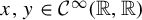
As in the Riemannian setting, we define the exponential map
 $\exp ^\unicode{x3bb} :TM\to M$
by
$\exp ^\unicode{x3bb} :TM\to M$
by
For every
 $x\in M$
, the map
$x\in M$
, the map
 $\exp _x^\unicode{x3bb} $
is
$\exp _x^\unicode{x3bb} $
is
 $\mathcal {C}^\infty $
on
$\mathcal {C}^\infty $
on
 $T_xM\setminus \{0\}$
but, in general, only
$T_xM\setminus \{0\}$
but, in general, only
 $\mathcal {C}^1$
at
$\mathcal {C}^1$
at
 $0$
; see, for instance, the proof of [Reference Dairbekov, Paternain, Stefanov and UhlmannDPSU07, Lemma A.7]. The lack of smoothness at the origin reflects the potential non-reversibility of thermostat flows. We say that the thermostat in question has no conjugate points if
$0$
; see, for instance, the proof of [Reference Dairbekov, Paternain, Stefanov and UhlmannDPSU07, Lemma A.7]. The lack of smoothness at the origin reflects the potential non-reversibility of thermostat flows. We say that the thermostat in question has no conjugate points if
 $\exp _x^\unicode{x3bb} $
is a local diffeomorphism for all
$\exp _x^\unicode{x3bb} $
is a local diffeomorphism for all
 $x\in M$
. Given a thermostat geodesic segment
$x\in M$
. Given a thermostat geodesic segment
 $\gamma : [0,T]\to M$
with distinct endpoints
$\gamma : [0,T]\to M$
with distinct endpoints ![]() and
and ![]() , we say that
, we say that
 $x_0$
and
$x_0$
and
 $x_1$
are conjugate along
$x_1$
are conjugate along
 $\gamma $
if the map
$\gamma $
if the map
 $\exp _{x_0}^\unicode{x3bb} $
is singular at
$\exp _{x_0}^\unicode{x3bb} $
is singular at
 $T\dot {\gamma }(0)$
, that is, if the differential
$T\dot {\gamma }(0)$
, that is, if the differential
 $d_{T\dot {\gamma }(0)}\exp _{x_0}^\unicode{x3bb} $
has a non-trivial kernel. The goal of this paper is to explain how the no-conjugate-points condition relates to different notions of curvature, as well as characterize the dynamics of such thermostats. In doing so, we highlight both the concepts that generalize perfectly from the geodesic case and the nuances that appear with greater dynamical complexity. This exercise not only sheds new light on thermostats, but also gives new results for geodesic flows.
$d_{T\dot {\gamma }(0)}\exp _{x_0}^\unicode{x3bb} $
has a non-trivial kernel. The goal of this paper is to explain how the no-conjugate-points condition relates to different notions of curvature, as well as characterize the dynamics of such thermostats. In doing so, we highlight both the concepts that generalize perfectly from the geodesic case and the nuances that appear with greater dynamical complexity. This exercise not only sheds new light on thermostats, but also gives new results for geodesic flows.
1.1 Conjugate points and thermostat curvature
Let
 $K_g\in \mathcal {C}^\infty (M, {\mathbb {R}})$
denote the Gaussian curvature of
$K_g\in \mathcal {C}^\infty (M, {\mathbb {R}})$
denote the Gaussian curvature of
 $(M,g)$
. In the geodesic case, it is easy to check that
$(M,g)$
. In the geodesic case, it is easy to check that
 $K_g \leq 0$
implies g has no conjugate points. The quantity that usually plays the role of Gaussian curvature for thermostats is the thermostat curvature
$K_g \leq 0$
implies g has no conjugate points. The quantity that usually plays the role of Gaussian curvature for thermostats is the thermostat curvature
 $\mathbb {K}\in \mathcal {C}^\infty (M, {\mathbb {R}})$
given by
$\mathbb {K}\in \mathcal {C}^\infty (M, {\mathbb {R}})$
given by
where ![]() . This is a smooth function on
. This is a smooth function on
 $SM$
instead of M. It turns out that this notion of thermostat curvature is implicitly making a choice of a gauge (see §2.1). Given a function
$SM$
instead of M. It turns out that this notion of thermostat curvature is implicitly making a choice of a gauge (see §2.1). Given a function
 $p: SM\to {\mathbb {R}}$
that is
$p: SM\to {\mathbb {R}}$
that is
 $\mathcal {C}^1$
along the flow, define
$\mathcal {C}^1$
along the flow, define
Observe that
 $\mathbb {K}$
corresponds to the special case
$\mathbb {K}$
corresponds to the special case
 $p=V\unicode{x3bb} $
. The quantity
$p=V\unicode{x3bb} $
. The quantity
 $\kappa _p$
was explicitly introduced in [Reference Mettler and PaternainMP19] as a tool for analyzing the dynamics of thermostat flows, but it already appears implicitly in [Reference Jane and PaternainJP09].
$\kappa _p$
was explicitly introduced in [Reference Mettler and PaternainMP19] as a tool for analyzing the dynamics of thermostat flows, but it already appears implicitly in [Reference Jane and PaternainJP09].
Our first result shows that the notion of curvature
 $\kappa _p$
offers a useful criterion to check whether a thermostat has no conjugate points.
$\kappa _p$
offers a useful criterion to check whether a thermostat has no conjugate points.
Theorem 1.1. Let
 $(M, g, \unicode{x3bb} )$
be a thermostat. If
$(M, g, \unicode{x3bb} )$
be a thermostat. If
 $\kappa _p\leq 0$
for some function
$\kappa _p\leq 0$
for some function
 $p:SM\to {\mathbb {R}}$
that is
$p:SM\to {\mathbb {R}}$
that is
 $\mathcal {C}^1$
along the flow, then there are no conjugate points.
$\mathcal {C}^1$
along the flow, then there are no conjugate points.
In fact, the additional degree of freedom that comes from the gauge p allows us to completely characterize thermostats without conjugate points. This characterization is also new for geodesic flows.
Theorem 1.2. A thermostat
 $(M, g, \unicode{x3bb} )$
has no conjugate points if and only if there exists a Borel measurable function
$(M, g, \unicode{x3bb} )$
has no conjugate points if and only if there exists a Borel measurable function
 $p: SM\to {\mathbb {R}}$
smooth along the flow with
$p: SM\to {\mathbb {R}}$
smooth along the flow with
 $\kappa _p=0$
.
$\kappa _p=0$
.
Next, we give a generalization of Hopf’s rigidity result in [Reference HopfHop48] to thermostats. Note that
 $\mu $
denotes the Liouville form on
$\mu $
denotes the Liouville form on
 $SM$
.
$SM$
.
Theorem 1.3. Let
 $(M, g, \unicode{x3bb} )$
be a thermostat without conjugate points. For any Borel measurable function
$(M, g, \unicode{x3bb} )$
be a thermostat without conjugate points. For any Borel measurable function
 $p: SM\to {\mathbb {R}}$
that is
$p: SM\to {\mathbb {R}}$
that is
 $\mathcal {C}^1$
along the flow, we have
$\mathcal {C}^1$
along the flow, we have
 $$ \begin{align} \int_{SM}\kappa_p \mu\leq \int_{SM}(p-V\unicode{x3bb})^2 \mu. \end{align} $$
Moreover, if equality holds, then
 $\mathbb {K}=0$
.
$\mathbb {K}=0$
.
As a consequence of the inequality (1.4) with
 $p=V\unicode{x3bb} $
, Stokes’s theorem, and the Gauss–Bonnet theorem, we get
$p=V\unicode{x3bb} $
, Stokes’s theorem, and the Gauss–Bonnet theorem, we get
 $$ \begin{align} 2\pi \chi(M)+\int_{SM}(\unicode{x3bb}^2-(V\unicode{x3bb})^2) \mu\leq 0, \end{align} $$
where
 $\chi (M)$
is the Euler characteristic of M. Furthermore, observe that the exponential map defined in (1.2) cannot yield a covering of the
$\chi (M)$
is the Euler characteristic of M. Furthermore, observe that the exponential map defined in (1.2) cannot yield a covering of the
 $2$
-sphere
$2$
-sphere
 $\mathbb {S}^2$
for topological reasons, so any surface admitting a thermostat without conjugate points must have genus at least one.
$\mathbb {S}^2$
for topological reasons, so any surface admitting a thermostat without conjugate points must have genus at least one.
Let us briefly focus on the case where
 $M $
is homeomorphic to the
$M $
is homeomorphic to the
 $2$
-torus
$2$
-torus
 $\mathbb {T}^2$
. In the geodesic case, we recover the classical fact by Hopf that g must be flat. In the magnetic case, the inequality (1.5) implies that
$\mathbb {T}^2$
. In the geodesic case, we recover the classical fact by Hopf that g must be flat. In the magnetic case, the inequality (1.5) implies that
 $\unicode{x3bb} = 0$
and then g must also be flat (see also [Reference Assenza, Marshall Reber and TerekAMT25, Corollary C]). In some sense, these observations are telling us that the situation on
$\unicode{x3bb} = 0$
and then g must also be flat (see also [Reference Assenza, Marshall Reber and TerekAMT25, Corollary C]). In some sense, these observations are telling us that the situation on
 $\mathbb {T}^2$
is very rigid when the flow is volume-preserving. If we allow
$\mathbb {T}^2$
is very rigid when the flow is volume-preserving. If we allow
 $\unicode{x3bb} $
to also have a linear term with respect to velocity, [Reference Assylbekov and DairbekovAD14, Theorem 1.1] tells us that the magnetic component of
$\unicode{x3bb} $
to also have a linear term with respect to velocity, [Reference Assylbekov and DairbekovAD14, Theorem 1.1] tells us that the magnetic component of
 $\unicode{x3bb} $
(that is, the zeroth Fourier mode
$\unicode{x3bb} $
(that is, the zeroth Fourier mode
 $\unicode{x3bb} _0$
) must still identically vanish and the metric g must be conformally flat. The following no-go result shows that this rigidity does not apply to more general thermostats on
$\unicode{x3bb} _0$
) must still identically vanish and the metric g must be conformally flat. The following no-go result shows that this rigidity does not apply to more general thermostats on
 $\mathbb {T}^2$
.
$\mathbb {T}^2$
.
Theorem 1.4. For any Riemannian metric g on
 $\mathbb {T}^2$
, there exists
$\mathbb {T}^2$
, there exists
 $\unicode{x3bb} \in \mathcal {C}^\infty (S\mathbb {T}^2, {\mathbb {R}})$
such that the thermostat
$\unicode{x3bb} \in \mathcal {C}^\infty (S\mathbb {T}^2, {\mathbb {R}})$
such that the thermostat
 $(\mathbb {T}^2, g, \unicode{x3bb} )$
has no conjugate points. Moreover, the function
$(\mathbb {T}^2, g, \unicode{x3bb} )$
has no conjugate points. Moreover, the function
 $\unicode{x3bb} $
can always be chosen such that
$\unicode{x3bb} $
can always be chosen such that
 $\unicode{x3bb} _0\neq 0$
.
$\unicode{x3bb} _0\neq 0$
.
1.2 Green bundles in the cotangent bundle
A key observation in the study of metrics without conjugate points is the existence of two flow-invariant subbundles of
 $T(SM)$
, known as Green bundles. The construction of these subbundles was extended to the setting of convex Hamiltonians in [Reference Contreras and IturriagaCI99]. However, these arguments do not directly carry over to the thermostat setting, as thermostats may be dissipative.
$T(SM)$
, known as Green bundles. The construction of these subbundles was extended to the setting of convex Hamiltonians in [Reference Contreras and IturriagaCI99]. However, these arguments do not directly carry over to the thermostat setting, as thermostats may be dissipative.
We take a new approach to understanding the Green bundles by working on the cotangent bundle
 $T^*(SM)$
as opposed to the tangent bundle
$T^*(SM)$
as opposed to the tangent bundle
 $T(SM)$
. The primary motivation is that, if we consider the induced dynamics, there is a smooth invariant subbundle
$T(SM)$
. The primary motivation is that, if we consider the induced dynamics, there is a smooth invariant subbundle
 $\Sigma \subset T^*(SM)$
which, in spirit, can replace the notion of a contact distribution in the geodesic case. Indeed, the symplectic lift of
$\Sigma \subset T^*(SM)$
which, in spirit, can replace the notion of a contact distribution in the geodesic case. Indeed, the symplectic lift of
 $\varphi _t$
to
$\varphi _t$
to
 $T^*(SM)$
, given by
$T^*(SM)$
, given by
is the Hamiltonian flow of
 $\xi (F(v))$
, so it preserves the characteristic set
$\xi (F(v))$
, so it preserves the characteristic set
 $\Sigma $
with fibers
$\Sigma $
with fibers
When working on
 $T^*(SM)$
, it is natural to introduce a moving coframe. The vector fields
$T^*(SM)$
, it is natural to introduce a moving coframe. The vector fields
 $(X, H, V)$
form an orthonormal frame for
$(X, H, V)$
form an orthonormal frame for
 $T(SM)$
with respect to the Sasaki metric (the natural lift of g to
$T(SM)$
with respect to the Sasaki metric (the natural lift of g to
 $SM$
). We can then consider the corresponding dual frame
$SM$
). We can then consider the corresponding dual frame
 $(\alpha , \beta , \psi )$
for
$(\alpha , \beta , \psi )$
for
 $T^*(SM)$
. The cohorizontal subbundle is defined as
$T^*(SM)$
. The cohorizontal subbundle is defined as ![]() , whereas the covertical is
, whereas the covertical is ![]() . In the geodesic case, we have
. In the geodesic case, we have
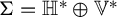 $\Sigma =\mathbb {H}^*\oplus \mathbb {V}^*$
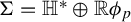
. For a thermostat, we introduce
$\Sigma =\mathbb {H}^*\oplus \mathbb {V}^*$
. For a thermostat, we introduce ![]() and
and ![]() so that
so that
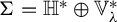 $\Sigma = \mathbb {H}^*\oplus \mathbb {V}^*_\unicode{x3bb} $
. See Figure 1.
$\Sigma = \mathbb {H}^*\oplus \mathbb {V}^*_\unicode{x3bb} $
. See Figure 1.
The adapted frame
 $(\alpha , \beta , \psi _\unicode{x3bb} )$
for
$(\alpha , \beta , \psi _\unicode{x3bb} )$
for
 $T^*(SM)$
.
$T^*(SM)$
.

In this new setting, we construct the Green bundles on orbits without conjugate points. Note that these are usually defined as subbundles of
 $T(SM)$
instead of
$T(SM)$
instead of
 $T^*(SM)$
.
$T^*(SM)$
.
Theorem 1.5. Let
 $(M, g, \unicode{x3bb} )$
be a thermostat. For a given
$(M, g, \unicode{x3bb} )$
be a thermostat. For a given
 $v\in SM$
, either of the following are observed.
$v\in SM$
, either of the following are observed.
-
(a) There exist
$t_0\in {\mathbb {R}}$
and
$t\neq 0$
such that (1.8)
$$ \begin{align} d\varphi_{t}^{-\top}({}\mathbb{H}^*(\varphi_{t_0}(v)))=\mathbb{H}^*(\varphi_{t_0+t}(v)). \end{align} $$
This happens if and only if the points
$\pi (\varphi _{t_0}(v))$
and
$\pi (\varphi _{t_0+t}(v))$
on M are conjugate along the thermostat geodesic
$t\mapsto \pi (\varphi _t(v))$
. -
(b) There exist two invariant subbundles
$G_{s/u}^*\subset \Sigma $
along the orbit of v given by (1.9)
$$ \begin{align} \begin{aligned} G^*_s(v):&=\lim_{t\to \infty}d\varphi_{-t}^{-\top}({}\mathbb{H}^*(\varphi_{t}(v))),\\ G^*_u(v):&=\lim_{t\to \infty}d\varphi_{t}^{-\top}({}\mathbb{H}^*(\varphi_{-t}(v))). \end{aligned} \end{align} $$
They satisfy the transversality condition
(1.10)
$$ \begin{align} G^*_s(v)\cap \mathbb{H}^*(v)=\{0\}=G^*_u(v)\cap \mathbb{H}^*(v). \end{align} $$


In [Reference EberleinEbe73, Theorem 3.2], Eberlein characterized Anosov geodesic flows as the geodesic flows without conjugate points that have transverse Green bundles. In [Reference Contreras and IturriagaCI99, Theorem C], a similar statement was given for convex Hamiltonians (which might be non-contact, but are still volume-preserving). Recall that a flow
 $\{\varphi _t\}_{t \in {\mathbb {R}}}$
is Anosov if there is a flow-invariant splitting
$\{\varphi _t\}_{t \in {\mathbb {R}}}$
is Anosov if there is a flow-invariant splitting
 $$ \begin{align*}T(SM) = {\mathbb{R}} F \oplus E_s \oplus E_u,\end{align*} $$
and constants
 $C \geq 1$
and
$C \geq 1$
and
 $0 < \rho < 1$
such that, for all
$0 < \rho < 1$
such that, for all
 $v\in SM$
and
$v\in SM$
and
 $t \geq 0$
, we have
$t \geq 0$
, we have
 $$ \begin{align} \Vert d_v\varphi_{t}|_{E_s(v)}\Vert \leq C\rho^t, \quad\Vert d_v\varphi_{-t}|_{E_u(v)}\Vert \leq C\rho^t. \end{align} $$
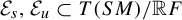
As we will see, due to the lack of volume preservation, the natural extension of these results to thermostats applies to projectively Anosov flows instead. The flow
 $\{\varphi _t\}_{t\in {\mathbb {R}}}$
is said to be projectively Anosov if there exist a flow-invariant splitting of the quotient tangent bundle
$\{\varphi _t\}_{t\in {\mathbb {R}}}$
is said to be projectively Anosov if there exist a flow-invariant splitting of the quotient tangent bundle
 $$ \begin{align*} T(SM)/{\mathbb{R}} F =\mathcal{E}_s\oplus \mathcal{E}_u, \end{align*} $$
and constants
 $C\geq 1$
and
$C\geq 1$
and
 $0 <\rho < 1$
such that, for any
$0 <\rho < 1$
such that, for any
 $v\in SM$
and
$v\in SM$
and
 $t\geq 0$
, we have
$t\geq 0$
, we have
 $$ \begin{align} \Vert d_v \varphi_t|_{\mathcal{E}_s(v)}\Vert \Vert d_{\varphi_t(v)}\varphi_{-t}|_{\mathcal{E}_u(\varphi_t(v))}\Vert\leq C \rho^t, \end{align} $$
where
 $\Vert \cdot \Vert $
denotes the operator norm induced by the Sasaki metric on
$\Vert \cdot \Vert $
denotes the operator norm induced by the Sasaki metric on
 $T(SM)$
. We assume that both subbundles
$T(SM)$
. We assume that both subbundles
 $\mathcal {E}_{s}, \mathcal {E}_u \subset T(SM)/{\mathbb {R}} F$
are non-trivial and we say that
$\mathcal {E}_{s}, \mathcal {E}_u \subset T(SM)/{\mathbb {R}} F$
are non-trivial and we say that
 $\mathcal {E}_u$
dominates
$\mathcal {E}_u$
dominates
 $\mathcal {E}_s$
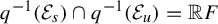
. These subbundles lift to flow-invariant subbundles
$\mathcal {E}_s$
. These subbundles lift to flow-invariant subbundles
 $q^{-1}(\mathcal {E}_s)$
and
$q^{-1}(\mathcal {E}_s)$
and
 $q^{-1}(\mathcal {E}_u)$
of
$q^{-1}(\mathcal {E}_u)$
of
 $T(SM)$
, where
$T(SM)$
, where
 $q: T(SM)\to T(SM)/{\mathbb {R}} F$
is the quotient map. We refer to them as the weak stable and unstable subbundles, respectively.
$q: T(SM)\to T(SM)/{\mathbb {R}} F$
is the quotient map. We refer to them as the weak stable and unstable subbundles, respectively.
Projectively Anosov flows also appear in the literature as conformally Anosov flows [Reference Eliashberg and ThurstonET98, Reference Blair and PeronneBP98] or as flows admitting a dominated splitting [Reference Arroyo and HertzAR03]. In the latter paper, the authors explain why this definition is the ‘adequate’ notion of dominated splitting for flows. This property does not appear in geodesic or magnetic settings because volume-preserving projectively Anosov flows are Anosov [Reference Araújo and PacificoAP10, Proposition 2.34]. In those cases, there is no need to differentiate between the notions. It is also worth noting that one could define the Anosov property directly on the quotient tangent bundle by requiring that the subbundles
 $\mathcal {E}_{s/u}$
satisfy the stronger estimates (1.11) instead of (1.12). These points of view are equivalent: in one direction, it suffices to take
$\mathcal {E}_{s/u}$
satisfy the stronger estimates (1.11) instead of (1.12). These points of view are equivalent: in one direction, it suffices to take ![]() and the converse is given by [Reference WojtkowskiWoj00a, Proposition 5.1].
and the converse is given by [Reference WojtkowskiWoj00a, Proposition 5.1].
The thermostat version of Eberlein’s result is hence the following theorem.
Theorem 1.6. Let
 $(M, g, \unicode{x3bb} )$
be a thermostat without conjugate points. It is projectively Anosov if and only if
$(M, g, \unicode{x3bb} )$
be a thermostat without conjugate points. It is projectively Anosov if and only if
 $G^*_s(v)\cap G^*_u(v)=\{0\}$
for all
$G^*_s(v)\cap G^*_u(v)=\{0\}$
for all
 $v\in SM$
.
$v\in SM$
.
Remark 1.7. In establishing the result for geodesic flows, Eberlein uses Klingenberg [Reference KlingenbergKli74] to argue that an Anosov geodesic flow must have no conjugate points. In the absence of such a result for projectively Anosov thermostats, we assume that the thermostat is without conjugate points.
For a projectively Anosov thermostat, we no longer have a direct sum decomposition of the tangent bundle, but only the weaker relation
 $$ \begin{align*}T(SM)=q^{-1}(\mathcal{E}_s)+ q^{-1}(\mathcal{E}_u)\end{align*} $$
with
 $q^{-1}(\mathcal {E}_s)\cap q^{-1}(\mathcal {E}_u)={\mathbb {R}} F$
. Nonetheless, we can still define the dual stable and unstable subbundles
$q^{-1}(\mathcal {E}_s)\cap q^{-1}(\mathcal {E}_u)={\mathbb {R}} F$
. Nonetheless, we can still define the dual stable and unstable subbundles
 $E^*_{s}, E^*_u\subset T^*(SM)$
via
$E^*_{s}, E^*_u\subset T^*(SM)$
via
 $$ \begin{align} E^*_s (q^{-1}(\mathcal{E}_{s}))=0=E^*_u(q^{-1}(\mathcal{E}_u)). \end{align} $$
With this definition, we then obtain the direct sum decomposition
 $$ \begin{align*}\Sigma = E^*_s \oplus E^*_u,\end{align*} $$
and
 $E^*_{s/u}$
satisfy analogues of the estimates (1.12), with
$E^*_{s/u}$
satisfy analogues of the estimates (1.12), with
 $d\varphi _t$
replaced by
$d\varphi _t$
replaced by
 $d\varphi _t^{-\top }$
. If the thermostat has no conjugate points and is projectively Anosov, then
$d\varphi _t^{-\top }$
. If the thermostat has no conjugate points and is projectively Anosov, then
 $G^*_{s/u}=E_{s/u}^*$
.
$G^*_{s/u}=E_{s/u}^*$
.
To prove Theorem 1.6, we use the following characterization of thermostats with transverse Green bundles. Interestingly, even in the well-studied geodesic case, it provides a new partial converse to [Reference AnosovAno67]: although the Anosov property does not imply negative Gaussian curvature [Reference Donnay and PughDP03, Reference Donnay and VisscherDV18], it does tell us that the thermostat curvature with respect to an appropriate gauge is negative everywhere.
Theorem 1.8. If a thermostat
 $(M,g,\unicode{x3bb} )$
without conjugate points has transverse Green bundles, there is a continuous function
$(M,g,\unicode{x3bb} )$
without conjugate points has transverse Green bundles, there is a continuous function
 $p : SM \to {\mathbb {R}}$
smooth along the flow with
$p : SM \to {\mathbb {R}}$
smooth along the flow with
 $\kappa _p < 0$
.
$\kappa _p < 0$
.
Finally, we explore the other extreme; namely, when the Green bundles collapse to a line everywhere instead of being transverse. For geodesic flows without conjugate points, a conjecture of Freire and Mañé can be rephrased as stating that the Green bundles collapse if and only if the metric is flat [Reference Freire and MañéFM82]. Note that, in the geodesic case, the Green bundles collapsing implies that the fundamental group grows sub-exponentially. However, then, if M is a surface, it must be the
 $2$
-sphere or the
$2$
-sphere or the
 $2$
-torus. The conjecture for surfaces then follows by [Reference HopfHop48].
$2$
-torus. The conjecture for surfaces then follows by [Reference HopfHop48].
A natural question is whether this extends to the thermostat setting with the thermostat curvature in place of the Gaussian curvature. As we will see in Proposition 4.1, this is not the case. In spite of this, there is still a connection between the Green bundles collapsing to a line, the thermostat curvature
 $\mathbb {K}$
, and a quantity which we refer to as the damped thermostat curvature,
$\mathbb {K}$
, and a quantity which we refer to as the damped thermostat curvature,
Note that
 $\tilde {\kappa }$
is simply
$\tilde {\kappa }$
is simply
 $\kappa _p$
with the particular choice of
$\kappa _p$
with the particular choice of
 $p=V\unicode{x3bb} /2$
.
$p=V\unicode{x3bb} /2$
.
Theorem 1.9. Let
 $(M, g, \unicode{x3bb} )$
be a thermostat.
$(M, g, \unicode{x3bb} )$
be a thermostat.
-
(a) If
$\mathbb {K} = 0$
, then the flow has no conjugate points and
$G^*_s=G^*_u = {\mathbb {R}}(\psi _\unicode{x3bb} - V(\unicode{x3bb} ) \beta )\ \mu $
-almost everywhere. Moreover, if
$V\unicode{x3bb} =0$
, then
$G^*_s=G^*_u = {\mathbb {R}}\psi _\unicode{x3bb} $
everywhere. -
(b) If
$\tilde {\kappa } \leq 0$
, then, for any invariant Borel measure
$\nu $
on
$SM$
, we have
$\tilde {\kappa }= 0\ \nu $
-almost everywhere if and only if
$ G^*_s=G^*_u\ \nu $
-almost everywhere.


In §4, we will show that Theorem 1.9(a) is optimal: when
 $V\unicode{x3bb} \neq 0$
, it is possible to have
$V\unicode{x3bb} \neq 0$
, it is possible to have
 $\mathbb {K}=0$
yet
$\mathbb {K}=0$
yet
 $G^*_s(v)\cap G^*_u(v)=\{0\}$
for some
$G^*_s(v)\cap G^*_u(v)=\{0\}$
for some
 $v\in SM$
. See Figure 2. In particular, this implies that the conjecture of Freire and Mañé does not extend to the setting of thermostats with the thermostat curvature in place of the Gaussian curvature. However, observe that if
$v\in SM$
. See Figure 2. In particular, this implies that the conjecture of Freire and Mañé does not extend to the setting of thermostats with the thermostat curvature in place of the Gaussian curvature. However, observe that if
 $V\unicode{x3bb} = 0$
(that is, the system is magnetic), then
$V\unicode{x3bb} = 0$
(that is, the system is magnetic), then
 $\mathbb {K} = \tilde {\kappa } = \kappa _0$
and
$\mathbb {K} = \tilde {\kappa } = \kappa _0$
and
 $\mu $
becomes an invariant measure for the thermostat flow. Thus, Theorem 1.9 implies the following result.
$\mu $
becomes an invariant measure for the thermostat flow. Thus, Theorem 1.9 implies the following result.
The lifted dynamics on the characteristic set
 $\Sigma $
.
$\Sigma $
.

Corollary 1.10. Let
 $(M,g,\unicode{x3bb} )$
be a magnetic system with
$(M,g,\unicode{x3bb} )$
be a magnetic system with
 $\kappa _0 \leq 0$
. We have
$\kappa _0 \leq 0$
. We have
 $\kappa _0 = 0$
if and only if
$\kappa _0 = 0$
if and only if
 $G_s^* = G_u^*$
everywhere.
$G_s^* = G_u^*$
everywhere.
Combining the above results with [Reference Dairbekov and PaternainDP07, Lemma 4.1] and [Reference Mettler and PaternainMP19, Proposition 3.5, Theorem 3.7], we have the following.

This should be contrasted with the following diagram, which summarizes what was previously known in the geodesic setting.

1.3 Remaining questions
As noted in Remark 1.7, it is not clear whether one needs the assumption that the thermostat is without conjugate points in Theorem 1.6. Given an Anosov flow on
 $SM$
, [Reference GhysGhy84, Theorem A] tells us that it is topologically orbit equivalent to the geodesic flow of any metric of constant negative Gaussian curvature on M. Therefore, these flows are transitive and their non-wandering set is all of
$SM$
, [Reference GhysGhy84, Theorem A] tells us that it is topologically orbit equivalent to the geodesic flow of any metric of constant negative Gaussian curvature on M. Therefore, these flows are transitive and their non-wandering set is all of
 $SM$
. This property ends up being critical in proving that there are no conjugate points. In contrast, as we will see with concrete examples in §4, projectively Anosov thermostats can have non-trivial wandering sets.
$SM$
. This property ends up being critical in proving that there are no conjugate points. In contrast, as we will see with concrete examples in §4, projectively Anosov thermostats can have non-trivial wandering sets.
Question. Can a projectively Anosov thermostat have conjugate points?
One possible approach to this problem is to try to understand thermostats on the
 $2$
-sphere
$2$
-sphere
 $\mathbb {S}^2$
. As pointed out above, it is easy to see using the exponential map that every such thermostat must have conjugate points. If one can construct an example which is projectively Anosov, then this would show that the projectively Anosov assumption is not enough to rule out conjugate points. However, it is not even clear whether there can be an arbitrary projectively Anosov flow on the unit tangent bundle of
$\mathbb {S}^2$
. As pointed out above, it is easy to see using the exponential map that every such thermostat must have conjugate points. If one can construct an example which is projectively Anosov, then this would show that the projectively Anosov assumption is not enough to rule out conjugate points. However, it is not even clear whether there can be an arbitrary projectively Anosov flow on the unit tangent bundle of
 $\mathbb {S}^2$
; the work of Arroyo and Rodríguez Hertz [Reference Arroyo and HertzAR03] gives some insight into the problem, but it does not seem to be enough to rule out such examples.
$\mathbb {S}^2$
; the work of Arroyo and Rodríguez Hertz [Reference Arroyo and HertzAR03] gives some insight into the problem, but it does not seem to be enough to rule out such examples.
Question. Does the unit tangent bundle of
 $\mathbb {S}^2$
admit a projectively Anosov flow?
$\mathbb {S}^2$
admit a projectively Anosov flow?
Another possible approach to this problem is to try to understand whether all projectively Anosov thermostats give rise to hyperbolic behavior. In §4, we give explicit examples of projectively Anosov thermostats on the
 $2$
-torus which are not Anosov, showing that this is not the case, and answering a question of Mettler and Paternain [Reference Mettler and PaternainMP19] about the existence of such systems. These examples critically rely on the fact that the surface is a
$2$
-torus which are not Anosov, showing that this is not the case, and answering a question of Mettler and Paternain [Reference Mettler and PaternainMP19] about the existence of such systems. These examples critically rely on the fact that the surface is a
 $2$
-torus and, thus, it may be possible that a projectively Anosov thermostat will always be Anosov if the surface is not the
$2$
-torus and, thus, it may be possible that a projectively Anosov thermostat will always be Anosov if the surface is not the
 $2$
-torus. In light of the previous question, one can try exploring the following question.
$2$
-torus. In light of the previous question, one can try exploring the following question.
Question. Is there a projectively Anosov thermostat on a surface of genus at least two which is not Anosov?
Next, we suspect that the assumption
 $\kappa _0\leq 0$
is not required in Corollary 1.10, and hence, the conjecture of Freire and Mañé does extend to the setting of magnetic systems on surfaces. Provided the function
$\kappa _0\leq 0$
is not required in Corollary 1.10, and hence, the conjecture of Freire and Mañé does extend to the setting of magnetic systems on surfaces. Provided the function
 $\unicode{x3bb} $
is sufficiently nice (that is, if the Mañé critical value is less than
$\unicode{x3bb} $
is sufficiently nice (that is, if the Mañé critical value is less than
 $1/2$
), one can use Theorem 1.3 and [Reference Burns and PaternainBP02b, Theorem D, Proposition 5.4] to deduce the result. It is not immediately obvious how to show that
$1/2$
), one can use Theorem 1.3 and [Reference Burns and PaternainBP02b, Theorem D, Proposition 5.4] to deduce the result. It is not immediately obvious how to show that
 $\kappa _0 = 0$
if one only assumes that the topological entropy is zero and the genus of M is at least two.
$\kappa _0 = 0$
if one only assumes that the topological entropy is zero and the genus of M is at least two.
Question. Let
 $(M,g,\unicode{x3bb} )$
be a magnetic system without conjugate points. Does
$(M,g,\unicode{x3bb} )$
be a magnetic system without conjugate points. Does
 $G_s^* = G_u^*$
everywhere imply
$G_s^* = G_u^*$
everywhere imply
 $\kappa _0 = 0$
?
$\kappa _0 = 0$
?
Based on part (b) of Theorem 1.9, it is possible that the damped thermostat curvature is better equipped for detecting the topological entropy of the thermostat flow. However, even in the setting where
 $\tilde {\kappa } \leq 0$
, it is not clear whether
$\tilde {\kappa } \leq 0$
, it is not clear whether
 $\tilde {\kappa } = 0$
everywhere is equivalent to the Green bundles collapsing everywhere.
$\tilde {\kappa } = 0$
everywhere is equivalent to the Green bundles collapsing everywhere.
Question. Let
 $(M,g,\unicode{x3bb} )$
be a thermostat. Is it the case that
$(M,g,\unicode{x3bb} )$
be a thermostat. Is it the case that
 $\tilde {\kappa } = 0$
if and only if
$\tilde {\kappa } = 0$
if and only if
 $G_s^*(v) = G_u^*(v)$
for all
$G_s^*(v) = G_u^*(v)$
for all
 $v\in SM$
?
$v\in SM$
?
1.4 Organization of the paper
In §2, we study the relationship between conjugate points, Green bundles, and thermostat curvature. We describe the lifted dynamics of the thermostat on the characteristic set in §2.1. In §2.2, we explain how our point of view is equivalent to the one using cocycles. The lifted dynamics gives us an interpretation of the no-conjugate-points condition in terms of the twist property of the cohorizontal subbundle in §2.3, unlocking Theorem 1.1. Next, in §2.4, we construct the Green bundles and prove Theorems 1.2, 1.3, and 1.5. We finish the section by studying the relationship between the Lyapunov exponents of the flow and the Green bundles in §2.5, giving us the tools to prove Theorem 1.9.
In §3, we explore the relationship between the projectively Anosov property and transverse Green bundles. We first show that transverse Green bundles must be continuous, and then use this property to prove Theorems 1.6 and 1.8.
In §4, we present a family of examples of thermostats on
 $\mathbb {T}^2$
without conjugate points that are projectively Anosov (yet are not Anosov), proving Theorem 1.4.
$\mathbb {T}^2$
without conjugate points that are projectively Anosov (yet are not Anosov), proving Theorem 1.4.
2 Conjugate points and Green bundles
In what follows,
 $(M, g)$
is a closed oriented Riemannian surface and we take an arbitrary
$(M, g)$
is a closed oriented Riemannian surface and we take an arbitrary
 $\unicode{x3bb} \in \mathcal {C}^\infty (SM, {\mathbb {R}})$
.
$\unicode{x3bb} \in \mathcal {C}^\infty (SM, {\mathbb {R}})$
.
2.1 Dynamics on the characteristic set
Recall that
 $(\alpha , \beta , \psi )$
is the global coframe for
$(\alpha , \beta , \psi )$
is the global coframe for
 $T^*(SM)$
dual to the orthonormal frame
$T^*(SM)$
dual to the orthonormal frame
 $(X, H, V)$
under the Sasaki metric. By using the commutation formulas,
$(X, H, V)$
under the Sasaki metric. By using the commutation formulas,
 $$ \begin{align*}[V,X]=H, \quad [V,H]=-X,\quad [X,H]=\pi^*(K_g)V, \end{align*} $$
we can derive the structure equations,
 $$ \begin{align*}d\alpha = \psi \wedge \beta, \quad d\beta=-\psi\wedge \alpha, \quad d\psi =-\pi^*(K_g)\alpha\wedge\beta.\end{align*} $$
We will use the adapted coframe
 $(\alpha , \beta , \psi _\unicode{x3bb} )$
. See Figure 1. Combining the previous structure equations with Cartan’s formula, we obtain
$(\alpha , \beta , \psi _\unicode{x3bb} )$
. See Figure 1. Combining the previous structure equations with Cartan’s formula, we obtain
 $$ \begin{align*} \mathcal{L}_{F}\alpha =\unicode{x3bb} \beta, \quad \mathcal{L}_{F}\beta =\psi_\unicode{x3bb}, \quad \mathcal{L}_{F}\psi_\unicode{x3bb} = -\kappa_0 \beta+V(\unicode{x3bb})\psi_\unicode{x3bb}, \end{align*} $$
where
 $\kappa _0$
is defined in (1.3) (with
$\kappa _0$
is defined in (1.3) (with
 $p=0$
).
$p=0$
).
For any function
 $p: SM\to {\mathbb {R}}$
that is
$p: SM\to {\mathbb {R}}$
that is
 $\mathcal {C}^1$
along the flow, it will also be useful to define
$\mathcal {C}^1$
along the flow, it will also be useful to define ![]() so that
so that
 $(\alpha , \beta , \phi _p)$
is an alternative coframe satisfying
$(\alpha , \beta , \phi _p)$
is an alternative coframe satisfying
 $\Sigma =\mathbb {H}^*\oplus {\mathbb {R}}\phi _p$
(see Figure 3). This is nothing but a change of coordinates on
$\Sigma =\mathbb {H}^*\oplus {\mathbb {R}}\phi _p$
(see Figure 3). This is nothing but a change of coordinates on
 $\Sigma $
. We now have
$\Sigma $
. We now have
 $$ \begin{align} \mathcal{L}_{F}\beta =p\beta+\phi_p, \quad \mathcal{L}_{F}\phi_p = -\kappa_p \beta + (V\unicode{x3bb} - p)\phi_p. \end{align} $$
The bases
 $(\beta , \psi _\unicode{x3bb} )$
and
$(\beta , \psi _\unicode{x3bb} )$
and
 $(\beta , \phi _p)$
for
$(\beta , \phi _p)$
for
 $\Sigma $
.
$\Sigma $
.

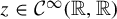
To each
 $\xi \in \Sigma (v)$
, we associate the functions
$\xi \in \Sigma (v)$
, we associate the functions
 $x,y\in \mathcal {C}^\infty ({\mathbb {R}}, {\mathbb {R}})$
characterized by
$x,y\in \mathcal {C}^\infty ({\mathbb {R}}, {\mathbb {R}})$
characterized by
 $$ \begin{align} d_v\varphi_t^{-\top}(\xi)= x(t)\beta+y(t)\phi_p. \end{align} $$
They capture all the information of the lifted dynamics in
 $\Sigma $
.
$\Sigma $
.
Lemma 2.1. Let
 $\xi \in \Sigma (v)$
. Along the orbit of v, we have the pair of equations
$\xi \in \Sigma (v)$
. Along the orbit of v, we have the pair of equations
 $$ \begin{align} \begin{cases} \dot{x}+px-\kappa_p y=0,\\ \dot{y}+x+(V\unicode{x3bb}-p)y = 0. \end{cases} \end{align} $$
In particular, the y component always satisfies the Jacobi equation
 $$ \begin{align} \ddot{y} + V(\unicode{x3bb})\dot{y}+\mathbb{K}y=0. \end{align} $$
Proof. By the definition of the inverse transpose
 $d_v\varphi _t^{-\top }$
, we have
$d_v\varphi _t^{-\top }$
, we have
if and only if
 $$ \begin{align*} \xi = \eta(t)\circ d_v\varphi_t. \end{align*} $$
Therefore, we may write
 $$ \begin{align*}\xi=x(t)\beta\circ d_v\varphi_t+y(t)\phi_p\circ d_v\varphi_t=x(t)\varphi_t^*\beta+y(t)\varphi_t^*\phi_p.\end{align*} $$
Differentiating this identity with respect to t and using the definition of the Lie derivative
 $\mathcal {L}_F$
, we obtain
$\mathcal {L}_F$
, we obtain
 $$ \begin{align*}0=\dot{x}\varphi_t^*\beta+x\varphi_t^*(\mathcal{L}_F \beta)+\dot{y}\varphi_t^*\phi_p+y\varphi_t^*(\mathcal{L}_F \phi_p).\end{align*} $$
Using (2.1), we see that
 $$ \begin{align*}0=(\dot{x}+px-\kappa_p y)\varphi_t^*\beta+(\dot{y}+x+(V\unicode{x3bb}-p)y)\varphi_t^*\phi_p.\end{align*} $$
Since
 $(\beta , \phi _p)$
are linearly independent, we get the pair of equations (2.3), as desired.
$(\beta , \phi _p)$
are linearly independent, we get the pair of equations (2.3), as desired.
Remark 2.2. Observe that this implies that x is completely determined by y.
For each
 $v\in SM$
, it will also be useful to introduce the damping function
$v\in SM$
, it will also be useful to introduce the damping function

Indeed, it allows us to associate to each
 $\xi \in \Sigma (v)$
a new function
$\xi \in \Sigma (v)$
a new function
 $z\in \mathcal {C}^\infty ({\mathbb {R}}, {\mathbb {R}})$
given by the relation
$z\in \mathcal {C}^\infty ({\mathbb {R}}, {\mathbb {R}})$
given by the relation
We think of z as a damped y component.
Lemma 2.3. For each
 $\xi \in \Sigma (v)$
, the z component is a solution of the Jacobi equation
$\xi \in \Sigma (v)$
, the z component is a solution of the Jacobi equation
 $$ \begin{align} \ddot{z}+ \tilde{\kappa} z = 0 \end{align} $$
along the orbit of v, where the quantity
 $\tilde {\kappa }$
is defined in (1.14).
$\tilde {\kappa }$
is defined in (1.14).
Proof. First, we use the fact that
 $y=mz$
to get
$y=mz$
to get
 $$ \begin{align*}\dot{y}=-\dfrac{V\unicode{x3bb}}{2}y+m\dot{z}.\end{align*} $$
Taking a second derivative, we obtain
 $$ \begin{align} \ddot{y} &=-\dfrac{FV\unicode{x3bb}}{2}y-\dfrac{V\unicode{x3bb}}{2}\bigg(-\dfrac{V\unicode{x3bb}}{2}y+m\dot{z}\bigg)- \dfrac{V\unicode{x3bb}}{2}m\dot{z}+m\ddot{z} \nonumber\\ &=m\bigg(-\dfrac{FV\unicode{x3bb}}{2}z+\dfrac{(V\unicode{x3bb})^2}{4}z-V(\unicode{x3bb})\dot{z}+\ddot{z}\bigg). \end{align} $$
However, the Jacobi equation (2.4) yields
 $$ \begin{align*} \begin{aligned} \ddot{y}&=-V(\unicode{x3bb})\dot{y}-(\kappa_0+FV\unicode{x3bb})y\\ &=m\bigg(\dfrac{(V\unicode{x3bb})^2}{2}z-V(\unicode{x3bb})\dot{z}-(\kappa_0+FV\unicode{x3bb})z\bigg).\\ \end{aligned} \end{align*} $$
Setting them equal to each other then gives us the claim since m is nowhere-vanishing.
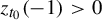
One of the advantages of studying the damped component z defined in (2.6) instead of y is that, thanks to Lemma 2.3, we are able to use the following general result when there are no conjugate points.
Lemma 2.4. Let
 $k\in \mathcal {C}^\infty ({\mathbb {R}})$
be such that any non-trivial solution z to the equation
$k\in \mathcal {C}^\infty ({\mathbb {R}})$
be such that any non-trivial solution z to the equation
 $$ \begin{align} \ddot{z}+kz=0 \end{align} $$
vanishes at most once. If such z vanishes once, then
 $|z(t)|$
is unbounded as
$|z(t)|$
is unbounded as
 $t\to \pm \infty $
.
$t\to \pm \infty $
.
Proof. By normalizing if needed, it suffices to consider the case where
 $z(0)=0$
and
$z(0)=0$
and
 $\dot {z}(0)=1$
. For each
$\dot {z}(0)=1$
. For each
 $t_0\neq 0$
, we know thanks to the one-time vanishing property and the homogeneity of (2.9) that there exists a unique solution
$t_0\neq 0$
, we know thanks to the one-time vanishing property and the homogeneity of (2.9) that there exists a unique solution
 $z_{t_0}$
with
$z_{t_0}$
with
 $z_{t_0}(0)=1$
and
$z_{t_0}(0)=1$
and
 $z_{t_0}(t_0)=0.$
We claim that
 $$ \begin{align*} z_{t_0}=z_{-1}+\dfrac{z_{t_0}(-1)}{z(-1)}z. \end{align*} $$
Indeed, since both sides satisfy (2.9), and agree at
 $t=-1$
and
$t=-1$
and
 $t=0$
, the one-time vanishing property tells us that they must agree for all
$t=0$
, the one-time vanishing property tells us that they must agree for all
 $t\in {\mathbb {R}}$
.
$t\in {\mathbb {R}}$
.
Differentiating with respect to t and setting
 $t=0$
, we obtain
$t=0$
, we obtain
 $$ \begin{align*}\dot{z}_{t_0}(0)=\dot{z}_{-1}(0)+\dfrac{z_{t_0}(-1)}{z(-1)}.\end{align*} $$
Now, let
 $t_0>0$
. Since
$t_0>0$
. Since
 $z_{t_0}(-1)>0$
and
$z_{t_0}(-1)>0$
and
 $z(-1)<0$
, we notice that
$z(-1)<0$
, we notice that
 $t_0\mapsto \dot {z}_{t_0}(0)$
is bounded above as
$t_0\mapsto \dot {z}_{t_0}(0)$
is bounded above as
 $t_0\to \infty $
. For
$t_0\to \infty $
. For
 $t>0$
, note that the function
$t>0$
, note that the function
 $$ \begin{align*} t\mapsto z(t)\int_t^{t_0} \dfrac{1}{(z(\tau))^2}\, d\tau \end{align*} $$
satisfies (2.9). Moreover, using a Taylor expansion, we can see that it tends to
 $1$
as
$1$
as
 $t\to 0$
. Since it also agrees with the function
$t\to 0$
. Since it also agrees with the function
 $z_{t_0}$
at
$z_{t_0}$
at
 $t=t_0$
, the one-time vanishing property yields
$t=t_0$
, the one-time vanishing property yields
 $$ \begin{align} z_{t_0}(t)=z(t)\int_t^{t_0} \dfrac{1}{(z(\tau))^2}\, d\tau \end{align} $$
for all
 $t\in {\mathbb {R}}$
. It follows that, for
$t\in {\mathbb {R}}$
. It follows that, for
 $t_0>t_0'>0$
, we have
$t_0>t_0'>0$
, we have
 $$ \begin{align} \dot{z}_{t_0}(0)-\dot{z}_{t_0'}(0)=\int_{t_0'}^{t_0}\dfrac{1}{(z(\tau))^2}\, d\tau>0, \end{align} $$
so
 $t_0\mapsto \dot {z}_{t_0}(0)$
is monotone increasing as
$t_0\mapsto \dot {z}_{t_0}(0)$
is monotone increasing as
 $t_0\to \infty $
. Combined with the previous upper bound, this implies that
$t_0\to \infty $
. Combined with the previous upper bound, this implies that
 $t_0\mapsto \dot {z}_{t_0}(0)$
converges, so we may take the limit
$t_0\mapsto \dot {z}_{t_0}(0)$
converges, so we may take the limit
 $t_0\to \infty $
in (2.11) to obtain a convergent integral on the right-hand side. We conclude that
$t_0\to \infty $
in (2.11) to obtain a convergent integral on the right-hand side. We conclude that
 $|z(t)|$
is unbounded as
$|z(t)|$
is unbounded as
 $t\to \infty $
. The same argument works for
$t\to \infty $
. The same argument works for
 $t\to -\infty $
if we instead take
$t\to -\infty $
if we instead take
 $t_0<0$
.
$t_0<0$
.
2.2 Cocyles
Using the global coframe
 $(\beta , \psi _\unicode{x3bb} )$
for the characteristic set
$(\beta , \psi _\unicode{x3bb} )$
for the characteristic set
 $\Sigma $
, we get an identification
$\Sigma $
, we get an identification
 $\Sigma \cong M\times {\mathbb {R}}^2$
. Therefore, for each
$\Sigma \cong M\times {\mathbb {R}}^2$
. Therefore, for each
 $t\in {\mathbb {R}}$
, we obtain a unique map
$t\in {\mathbb {R}}$
, we obtain a unique map
 ${\Psi _t: SM\to \text {GL}(n,{\mathbb {R}})}$
characterized by
${\Psi _t: SM\to \text {GL}(n,{\mathbb {R}})}$
characterized by
 $$ \begin{align*}\tilde{\varphi}_t(v, \xi)=(\varphi_t(v), \Psi_t(v)\xi)\end{align*} $$
for all
 $(v, \xi )\in \Sigma \cong M\times {\mathbb {R}}^2$
. The map
$(v, \xi )\in \Sigma \cong M\times {\mathbb {R}}^2$
. The map
 $\Psi :SM\times {\mathbb {R}}\to \text {GL}(2,{\mathbb {R}})$
satisfies the cocycle property over the flow
$\Psi :SM\times {\mathbb {R}}\to \text {GL}(2,{\mathbb {R}})$
satisfies the cocycle property over the flow
 $\{\varphi _t\}_{t\in {\mathbb {R}}}$
, that is,
$\{\varphi _t\}_{t\in {\mathbb {R}}}$
, that is,
 $$ \begin{align*}\Psi_{t+s}(v)=\Psi_s(\varphi_t(v))\Psi_t(v)\end{align*} $$
for all
 $t, s\in {\mathbb {R}}$
. This is simply a different point of view of the previous subsection, with the explicit relationship given by
$t, s\in {\mathbb {R}}$
. This is simply a different point of view of the previous subsection, with the explicit relationship given by
 $$ \begin{align*} \Psi_t(v) \begin{pmatrix} x(0) \\ y(0) \end{pmatrix} = \begin{pmatrix} x(t) \\ y(t) \end{pmatrix}\!, \end{align*} $$
where the x and y components satisfy the differential equations (2.3). If we denote by
 $\Phi : SM\to \mathfrak {gl}(2, {\mathbb {R}})$
the infinitesimal generator of
$\Phi : SM\to \mathfrak {gl}(2, {\mathbb {R}})$
the infinitesimal generator of
 $\{\Psi _t\}_{t\in {\mathbb {R}}}$
, namely,
$\{\Psi _t\}_{t\in {\mathbb {R}}}$
, namely,

then (2.3) with
 $p=0$
allows us to explicitly write
$p=0$
allows us to explicitly write
 $$ \begin{align*}\Phi = \begin{pmatrix} 0 & \kappa_0 \\ -1 & -V\unicode{x3bb} \end{pmatrix}\!.\end{align*} $$
Of course, we could have made a different choice of global coframe on
 $\Sigma $
. This is represented by a gauge, that is, a smooth map
$\Sigma $
. This is represented by a gauge, that is, a smooth map
 $P:SM\to \text {GL}(2, {\mathbb {R}})$
, which gives rise to a new cocyle over the flow
$P:SM\to \text {GL}(2, {\mathbb {R}})$
, which gives rise to a new cocyle over the flow
 $\{\varphi _t\}_{t\in {\mathbb {R}}}$
by conjugation:
$\{\varphi _t\}_{t\in {\mathbb {R}}}$
by conjugation:
 $$ \begin{align*}\widetilde{\Psi}_t(v)=P^{-1}(\varphi_t(v))\Psi_t(v)P(v). \end{align*} $$
One can check that the new infinitesimal generator
 $\widetilde {\Phi }$
is related to
$\widetilde {\Phi }$
is related to
 $\Phi $
by
$\Phi $
by
 $$ \begin{align*} \widetilde{\Phi}=P^{-1}(\Phi + F) P. \end{align*} $$
Under this lens, our previous choice of coframe
 $(\beta , \phi _p)$
corresponds to the gauge
$(\beta , \phi _p)$
corresponds to the gauge
 $$ \begin{align*} P=\begin{pmatrix} 1 & 0 \\ -p & 1 \end{pmatrix}\!, \end{align*} $$
and the infinitesimal generator of the new cocyle
 $\{\widetilde {\Psi }_t\}_{t\in {\mathbb {R}}}$
becomes
$\{\widetilde {\Psi }_t\}_{t\in {\mathbb {R}}}$
becomes
 $$ \begin{align*} \widetilde{\Phi} = \begin{pmatrix} -p & \kappa_p \\ -1 & p-V\unicode{x3bb} \end{pmatrix}\!. \end{align*} $$
Note in particular that, for
 $p=V\unicode{x3bb} /2$
, we may rewrite this as
$p=V\unicode{x3bb} /2$
, we may rewrite this as
 $$ \begin{align} \widetilde{\Phi} = - \frac{V\unicode{x3bb}}{2} \text{Id} + \begin{pmatrix} 0 & \tilde{\kappa} \\ -1 & 0 \end{pmatrix}\!, \end{align} $$
so that
 $$ \begin{align} \widetilde{\Psi}_t(v) = m(t) \Gamma_t(v), \end{align} $$
where the damping function m is defined in (2.5) and
 $\{\Gamma _t\}_{t\in {\mathbb {R}}}$
is the cocycle generated by the last matrix in (2.12). In light of Lemma 2.3, we have
$\{\Gamma _t\}_{t\in {\mathbb {R}}}$
is the cocycle generated by the last matrix in (2.12). In light of Lemma 2.3, we have
 $$ \begin{align*} \Gamma_t(v) \begin{pmatrix} x(0) \\ z(0) \end{pmatrix} = \begin{pmatrix} x(t) \\ z(t) \end{pmatrix}\!. \end{align*} $$
Note that the infinitesimal generator of
 $\{\Gamma _t\}_{t\in {\mathbb {R}}}$
has trace zero, so
$\{\Gamma _t\}_{t\in {\mathbb {R}}}$
has trace zero, so
 $\Gamma _t: SM\to \text {SL}(2,{\mathbb {R}})$
. This is essentially the same cocyle as the one we would get from a geodesic flow with ‘Gaussian curvature’
$\Gamma _t: SM\to \text {SL}(2,{\mathbb {R}})$
. This is essentially the same cocyle as the one we would get from a geodesic flow with ‘Gaussian curvature’
 $\tilde {\kappa }$
; however, note that
$\tilde {\kappa }$
; however, note that
 $\tilde {\kappa }$
is a function on
$\tilde {\kappa }$
is a function on
 $SM$
instead of M. By picking the right gauge and damping the y component in the cotangent bundle, we are hence reducing the problem to something that resembles the geodesic case.
$SM$
instead of M. By picking the right gauge and damping the y component in the cotangent bundle, we are hence reducing the problem to something that resembles the geodesic case.
2.3 Conjugate points
In the geodesic case, the definition of conjugate points is often formulated in terms of a Jacobi equation. Let us restate our previous definition of conjugate points in terms of a Jacobi equation for thermostats.
Lemma 2.5. Let
 $\gamma : [0,T] \rightarrow M$
be a thermostat geodesic segment with distinct endpoints
$\gamma : [0,T] \rightarrow M$
be a thermostat geodesic segment with distinct endpoints
 $x_0=\gamma (0)$
and
$x_0=\gamma (0)$
and
 $x_1=\gamma (T)$
. The points
$x_1=\gamma (T)$
. The points
 $x_0$
and
$x_0$
and
 $x_1$
are conjugate along
$x_1$
are conjugate along
 $\gamma $
if and only if there exists a non-trivial solution y to the Jacobi equation (2.4) satisfying
$\gamma $
if and only if there exists a non-trivial solution y to the Jacobi equation (2.4) satisfying
 $y(0) = y(T) = 0$
.
$y(0) = y(T) = 0$
.
Proof. Since the function m defined in (2.5) is nowhere-vanishing, we have
 $y(t)=0$
if and only if
$y(t)=0$
if and only if
 $z(t)=0$
. We can thus conclude by applying Lemma 2.3 and [Reference Assylbekov and DairbekovAD14, Theorem 4.3]. Indeed, while their Jacobi equation for y is different from (2.4) because they are working in the tangent bundle, the authors show in [Reference Assylbekov and DairbekovAD14, §5] that a change of variables puts their Jacobi equation in the same normal form as (2.7).
$z(t)=0$
. We can thus conclude by applying Lemma 2.3 and [Reference Assylbekov and DairbekovAD14, Theorem 4.3]. Indeed, while their Jacobi equation for y is different from (2.4) because they are working in the tangent bundle, the authors show in [Reference Assylbekov and DairbekovAD14, §5] that a change of variables puts their Jacobi equation in the same normal form as (2.7).
Corollary 2.6. A thermostat has no conjugate points if and only if there are no non-trivial solutions to the Jacobi equation (2.4) (or (2.7)) which vanish at two distinct points.
Remark 2.7. There is a nice geometric interpretation of what is going on in the cotangent bundle. Note that having
 $y(t)=0$
is equivalent to
$y(t)=0$
is equivalent to
 $d_v\varphi _t^{-\top }(\xi )\in \mathbb {H}^*(\varphi _t(v))$
, so we get part (a) of Theorem 1.5. See Figure 2(a).
$d_v\varphi _t^{-\top }(\xi )\in \mathbb {H}^*(\varphi _t(v))$
, so we get part (a) of Theorem 1.5. See Figure 2(a).
Armed with this perspective on conjugate points, we prove Theorem 1.1.
Proof of Theorem 1.1
Let z be a non-trivial solution to the Jacobi equation (2.7) and define

By Lemma 2.3, we have
 $$ \begin{align*} \dot{w}&=\dot{z}^2-2\bigg(p-\dfrac{V\unicode{x3bb}}{2}\bigg)\dot{z}z- \bigg(\tilde{\kappa}+F\bigg(p-\dfrac{V\unicode{x3bb}}{2}\bigg)\bigg)z^2\\ &=\bigg(\dot{z}-\bigg(p-\dfrac{V\unicode{x3bb}}{2}\bigg)z\bigg)^2-\bigg(\tilde{\kappa}+ F\bigg(p-\dfrac{V\unicode{x3bb}}{2}\bigg)+\bigg(p-\dfrac{V\unicode{x3bb}}{2}\bigg)^2\bigg)z^2\\ &=\bigg(\dot{z}-\bigg(p-\dfrac{V\unicode{x3bb}}{2}\bigg)z\bigg)^2-\kappa_p z^2. \end{align*} $$
Since
 $\kappa _p \leq 0$
by assumption, we get
$\kappa _p \leq 0$
by assumption, we get
 $\dot {w}\geq 0,$
so the function w is non-decreasing. Suppose for contradiction, using Corollary 2.6, that z vanishes multiple times. Note that, because of the Jacobi equation (2.7), if z vanishes on an interval, then we must have
$\dot {w}\geq 0,$
so the function w is non-decreasing. Suppose for contradiction, using Corollary 2.6, that z vanishes multiple times. Note that, because of the Jacobi equation (2.7), if z vanishes on an interval, then we must have
 $z = 0$
everywhere; thus, we may assume that z vanishes on a discrete set. Let
$z = 0$
everywhere; thus, we may assume that z vanishes on a discrete set. Let
 $t_0 \in {\mathbb {R}}$
be such that
$t_0 \in {\mathbb {R}}$
be such that
 $z(t_0) = 0$
and let
$z(t_0) = 0$
and let ![]() . If
. If
 $t_1 = t_0$
, then we have an infinite sequence
$t_1 = t_0$
, then we have an infinite sequence
 $t_n \to t_0^+$
such that
$t_n \to t_0^+$
such that
 $z(t_n) = 0$
. By the mean value theorem, we get a sequence
$z(t_n) = 0$
. By the mean value theorem, we get a sequence
 $t_n' \to t_0^+$
with
$t_n' \to t_0^+$
with
 $\dot {z}(t_n') = 0$
and hence,
$\dot {z}(t_n') = 0$
and hence,
 $\dot {z}(t_0) = z(t_0) = 0$
by continuity, forcing z to be zero everywhere. Thus, we must have
$\dot {z}(t_0) = z(t_0) = 0$
by continuity, forcing z to be zero everywhere. Thus, we must have
 $t_1> t_0$
.
$t_1> t_0$
.
By construction, z does not vanish on the interval
 $(t_0, t_1)$
. Since w is non-decreasing and
$(t_0, t_1)$
. Since w is non-decreasing and
 $w(t_0)=w(t_1)=0$
, w must vanish on this interval. Then, however, z solves the first-order differential equation
$w(t_0)=w(t_1)=0$
, w must vanish on this interval. Then, however, z solves the first-order differential equation
 $\dot {z}=(p-V\unicode{x3bb} /2)z$
on
$\dot {z}=(p-V\unicode{x3bb} /2)z$
on
 $(t_0,t_1)$
with
$(t_0,t_1)$
with
 $z(t_0) = z(t_1) = 0$
; it is easy to see that this implies that
$z(t_0) = z(t_1) = 0$
; it is easy to see that this implies that
 $z = 0$
on the interval, which is a contradiction.
$z = 0$
on the interval, which is a contradiction.
2.4 Green bundles
Next, we want to show that having no conjugate points implies that the subbundle
 $d\varphi _t^{-\top }( \mathbb {H}^*(\varphi _{-t}(v)))$
converges as
$d\varphi _t^{-\top }( \mathbb {H}^*(\varphi _{-t}(v)))$
converges as
 $t \rightarrow \pm \infty $
. In this paper, when we talk about convergence of subbundles, we mean it in the sense that the subbundles converge in the Grassmannian topology of the projective bundle
$t \rightarrow \pm \infty $
. In this paper, when we talk about convergence of subbundles, we mean it in the sense that the subbundles converge in the Grassmannian topology of the projective bundle
 $\mathbb {P}(\Sigma )$
(also called the Grassmann 1-plane bundle) of the vector bundle
$\mathbb {P}(\Sigma )$
(also called the Grassmann 1-plane bundle) of the vector bundle
 $\Sigma \to SM$
. That is,
$\Sigma \to SM$
. That is,
 $\mathbb {P}(\Sigma )$
is the four-dimensional manifold obtained by projectivizing
$\mathbb {P}(\Sigma )$
is the four-dimensional manifold obtained by projectivizing
 $\Sigma (v)$
for each
$\Sigma (v)$
for each
 $v\in SM$
: the fiber over v consists of all one-dimensional subspaces of
$v\in SM$
: the fiber over v consists of all one-dimensional subspaces of
 $\Sigma (v)$
. Note that both
$\Sigma (v)$
. Note that both
 $\mathbb {V}^*$
and
$\mathbb {V}^*$
and
 $\mathbb {H}^*$
define sections of this bundle. The flow
$\mathbb {H}^*$
define sections of this bundle. The flow
 $\{\tilde {\varphi }_t\}_{t\in {\mathbb {R}}}$
on
$\{\tilde {\varphi }_t\}_{t\in {\mathbb {R}}}$
on
 $T^*(SM)$
naturally induces a flow on
$T^*(SM)$
naturally induces a flow on
 $\mathbb {P}(\Sigma )$
, which we continue to denote by the same symbol.
$\mathbb {P}(\Sigma )$
, which we continue to denote by the same symbol.
Proof of Theorem 1.5
Fix
 $v\in SM$
. We have already shown part (a), so in what follows, we may assume that
$v\in SM$
. We have already shown part (a), so in what follows, we may assume that
 $t\mapsto \pi (\varphi _t(v))$
contains no conjugate points on M. Equivalently, any solution z to the Jacobi equation (2.7) vanishes at most once.
$t\mapsto \pi (\varphi _t(v))$
contains no conjugate points on M. Equivalently, any solution z to the Jacobi equation (2.7) vanishes at most once.
Let
 $z_{t_0}$
be as in the proof of Lemma 2.4. Using Remark 2.2, we see that
$z_{t_0}$
be as in the proof of Lemma 2.4. Using Remark 2.2, we see that
 $z_{t_0}$
uniquely determines a point
$z_{t_0}$
uniquely determines a point
 $\xi _{t_0} \in \Sigma (v)$
so that
$\xi _{t_0} \in \Sigma (v)$
so that
 ${\mathbb {R}} \xi _{t_0} = d\varphi _{t_0}^{-\top }( \mathbb {H}^*(\varphi _{-t_0}(v)))$
. Note that the proof of Lemma 2.4 shows that
${\mathbb {R}} \xi _{t_0} = d\varphi _{t_0}^{-\top }( \mathbb {H}^*(\varphi _{-t_0}(v)))$
. Note that the proof of Lemma 2.4 shows that
 $\dot {z}_{t_0}(0)$
converges as
$\dot {z}_{t_0}(0)$
converges as
 $t_0 \rightarrow \pm \infty $
. Using the continuous dependence of solutions to (2.7) on initial conditions, we have that the functions
$t_0 \rightarrow \pm \infty $
. Using the continuous dependence of solutions to (2.7) on initial conditions, we have that the functions
 $z_{t_0}$
converge as
$z_{t_0}$
converge as
 $t_0 \rightarrow \pm \infty $
to solutions
$t_0 \rightarrow \pm \infty $
to solutions
 $z_{\pm \infty }$
of (2.7) whose corresponding points
$z_{\pm \infty }$
of (2.7) whose corresponding points
 $\xi _{\pm \infty } \in \Sigma (v)$
must span
$\xi _{\pm \infty } \in \Sigma (v)$
must span
 $\lim _{t_0 \rightarrow \pm \infty }\,d\varphi _{t_0}^{-\top }( \mathbb {H}^*(\varphi _{-t_0}(v)))$
and the result follows. The transversality condition (1.10) is then a direct consequence of Lemma 2.1 and the no-conjugate-points assumption.
$\lim _{t_0 \rightarrow \pm \infty }\,d\varphi _{t_0}^{-\top }( \mathbb {H}^*(\varphi _{-t_0}(v)))$
and the result follows. The transversality condition (1.10) is then a direct consequence of Lemma 2.1 and the no-conjugate-points assumption.
Thus, if a thermostat has no conjugate points, then for each
 $v\in SM$
, we can define
$v\in SM$
, we can define
 $G^*_{s/u}(v)\subset \Sigma (v)$
by the limiting procedures (1.9). Thanks to the transversality condition (1.10), we see that for each Borel measurable function
$G^*_{s/u}(v)\subset \Sigma (v)$
by the limiting procedures (1.9). Thanks to the transversality condition (1.10), we see that for each Borel measurable function
 $p: SM\to {\mathbb {R}}$
that is smooth in the direction of the flow, there exist functions
$p: SM\to {\mathbb {R}}$
that is smooth in the direction of the flow, there exist functions
 $r^s, r^u : SM \rightarrow {\mathbb {R}}$
so that
$r^s, r^u : SM \rightarrow {\mathbb {R}}$
so that
 $$ \begin{align} r^{s/u} \beta + \phi_p \in G_{s/u}^*. \end{align} $$
In general, these functions are Borel measurable. Still, as the next lemma shows, they satisfy a Riccati equation in the flow direction, in which they are always smooth.
Lemma 2.8. Let
 $(M, g, \unicode{x3bb} )$
be a thermostat without conjugate points. For each Borel measurable function
$(M, g, \unicode{x3bb} )$
be a thermostat without conjugate points. For each Borel measurable function
 $p: SM\to {\mathbb {R}}$
smooth in the direction of the flow, the functions
$p: SM\to {\mathbb {R}}$
smooth in the direction of the flow, the functions
 $r=r^{s/u}$
characterized by (2.14) satisfy the Riccati equation
$r=r^{s/u}$
characterized by (2.14) satisfy the Riccati equation
 $$ \begin{align} r^2 + (V\unicode{x3bb}-2p)r + \kappa_p - Fr = 0. \end{align} $$
Proof. Let us write
 $G^*$
for either
$G^*$
for either
 $G^*_{s}$
or
$G^*_{s}$
or
 $G^*_u$
. For notational convenience, let us also fix
$G^*_u$
. For notational convenience, let us also fix
 $v \in SM$
and define
$v \in SM$
and define ![]() ,
, ![]() , and
, and ![]() . If
. If ![]() then
then
 $\eta (t)\in G^*(v)$
for all
$\eta (t)\in G^*(v)$
for all
 $t\in {\mathbb {R}}$
. Unraveling the definitions, this means that
$t\in {\mathbb {R}}$
. Unraveling the definitions, this means that
 $$ \begin{align*}d_v\varphi_{t}^{-\top}(\eta(t))=r(t)\beta(t)+\phi_p(t),\end{align*} $$
and therefore,
 $$ \begin{align*}\eta(t)=r(t)\varphi_t^*\beta(t) +\varphi_t^*\phi_p(t).\end{align*} $$
Differentiating with respect to t and setting
 $t=0$
, we can use (2.1) to write
$t=0$
, we can use (2.1) to write
 $$ \begin{align*} \begin{aligned} \dot{\eta}(0) &=\dot{r}\beta+r\mathcal{L}_F\beta + \mathcal{L}_F\phi_p\\ & = (\dot{r} + r p - \kappa_p)\beta + (V\unicode{x3bb} - p + r)\phi_p. \end{aligned} \end{align*} $$
Since
 $\eta (0)=r\beta + \phi _p$
, we obtain
$\eta (0)=r\beta + \phi _p$
, we obtain
 $$ \begin{align*}\dot{\eta}(0)-(V\unicode{x3bb}-p + r)\eta(0)=(\dot{r} - \kappa_p - r V\unicode{x3bb}+2rp- r^2)\beta.\end{align*} $$
The left-hand side belongs to
 $G^*$
. We also know that
$G^*$
. We also know that
 $G^*$
is transverse to
$G^*$
is transverse to
 $\mathbb {H}^*$
, so the right-hand side must be zero. The claim follows.
$\mathbb {H}^*$
, so the right-hand side must be zero. The claim follows.
We can now prove Theorem 1.2.
Proof of Theorem 1.2
One direction is given by Theorem 1.1. In the other direction, suppose the thermostat has no conjugate points. Then, by picking
 $p=V\unicode{x3bb} $
in the Riccati equation (2.15), Lemma 2.8 gives us a Borel measurable function r smooth along the flow such that
$p=V\unicode{x3bb} $
in the Riccati equation (2.15), Lemma 2.8 gives us a Borel measurable function r smooth along the flow such that
 $$ \begin{align*}r^2-rV\unicode{x3bb} + \kappa_0 + FV\unicode{x3bb}-Fr=0.\end{align*} $$
If we now define ![]() , we get
, we get
 $$ \begin{align*}\kappa_p=\kappa_0 + Fp+p(p-V\unicode{x3bb})=0,\end{align*} $$
as desired.
We also have the tools to prove Theorem 1.3.
Proof of Theorem 1.3
Recall that
 $\text {div}_\mu F = V\unicode{x3bb} $
. By Stokes’s theorem, we have
$\text {div}_\mu F = V\unicode{x3bb} $
. By Stokes’s theorem, we have
 $$ \begin{align*}\int_{SM}F(r)\mu = -\int_{SM}rV(\unicode{x3bb}) \mu.\end{align*} $$
Integrating the Riccati equation (2.15), we hence get
 $$ \begin{align*}\int_{SM}(r^2+2(V\unicode{x3bb}-p)r)\mu =-\int_{SM}\kappa_p\mu.\end{align*} $$
It follows that
 $$ \begin{align} \int_{SM}(\kappa_p - (p-V\unicode{x3bb})^2) \mu &= -\int_{SM}(r^2+2(V\unicode{x3bb}-p)r+(p-V\unicode{x3bb})^2) \mu \nonumber\\ &=-\int_{SM}(r+V\unicode{x3bb}-p)^2\mu\leq 0. \end{align} $$
If the left-hand side is zero, then
 $r=p-V\unicode{x3bb} \mu $
-almost everywhere. Now, consider
$r=p-V\unicode{x3bb} \mu $
-almost everywhere. Now, consider
Since the flow
 $\{\varphi _t\}_{t\in {\mathbb {R}}}$
is smooth, the Radon–Nikodym theorem implies that the subset
$\{\varphi _t\}_{t\in {\mathbb {R}}}$
is smooth, the Radon–Nikodym theorem implies that the subset
 $B_t$
has full measure for every
$B_t$
has full measure for every
 $t \in {\mathbb {R}}$
, and hence, the intersection
$t \in {\mathbb {R}}$
, and hence, the intersection
 $ B_0 \cap (\bigcap _{n \geq 1} B_{1/n})$
also has full measure. Thus, we see that, for
$ B_0 \cap (\bigcap _{n \geq 1} B_{1/n})$
also has full measure. Thus, we see that, for
 $\mu $
-almost every
$\mu $
-almost every
 $v \in SM$
, we have
$v \in SM$
, we have
 $$ \begin{align*} \begin{aligned} (Fr)(v) &= \lim_{n \rightarrow \infty} n (r(\varphi_{1/n}(v)) - r(v)) \\ &= \lim_{n \rightarrow \infty} n (p(\varphi_{1/n}(v))- (V\unicode{x3bb})(\varphi_{1/n}(v)) - p(v) + (V\unicode{x3bb})(v)) \\ &= F(p-V\unicode{x3bb})(v). \end{aligned} \end{align*} $$
Substituting this into the Riccati equation (2.15) yields
 $\mathbb {K}=0\ \mu $
-almost everywhere. Since
$\mathbb {K}=0\ \mu $
-almost everywhere. Since
 $\mathbb {K}$
is a smooth function, we get
$\mathbb {K}$
is a smooth function, we get
 $\mathbb {K}=0$
everywhere.
$\mathbb {K}=0$
everywhere.
In fact, a slight modification of this argument yields the following, which will be useful in the proof of Theorem 1.9.
Lemma 2.9. Let
 $(M,g,\unicode{x3bb} )$
be a thermostat without conjugate points. For any finite flow-invariant Borel measure
$(M,g,\unicode{x3bb} )$
be a thermostat without conjugate points. For any finite flow-invariant Borel measure
 $\nu $
on
$\nu $
on
 $SM$
, we have
$SM$
, we have
 $$ \begin{align*} \int_{SM} \tilde{\kappa} \, d\nu \leq 0, \end{align*} $$
with equality if and only if
 $\tilde {\kappa } = 0\ \nu $
-almost everywhere.
$\tilde {\kappa } = 0\ \nu $
-almost everywhere.
Proof. Taking
 $p = V\unicode{x3bb} /2$
and integrating the Riccati equation (2.15) with respect to the measure
$p = V\unicode{x3bb} /2$
and integrating the Riccati equation (2.15) with respect to the measure
 $\nu $
, we get
$\nu $
, we get
 $$ \begin{align*} \int_{SM} \tilde{\kappa}\, d\nu = - \int_{SM} r^2\, d\nu \leq 0. \end{align*} $$
The left-hand side is zero if and only if r is zero
 $\nu $
-almost everywhere. With the same argument as in the proof of Theorem 1.3, we notice that having
$\nu $
-almost everywhere. With the same argument as in the proof of Theorem 1.3, we notice that having
 $r=0\ \nu $
-almost everywhere implies that
$r=0\ \nu $
-almost everywhere implies that
 $Fr=0\ \nu $
-almost everywhere. It then follows that
$Fr=0\ \nu $
-almost everywhere. It then follows that
 $\tilde {\kappa }=0\ \nu $
-almost everywhere.
$\tilde {\kappa }=0\ \nu $
-almost everywhere.
2.5 Lyapunov exponents
Recall that the Lyapunov exponent at
 $(v, \xi ) \in \Sigma $
is
$(v, \xi ) \in \Sigma $
is
where
 $\Vert \cdot \Vert $
is any continuous metric norm on
$\Vert \cdot \Vert $
is any continuous metric norm on
 $\Sigma $
. We use
$\Sigma $
. We use ![]() , where x and y are the adapted coordinates given by (2.2). Let
, where x and y are the adapted coordinates given by (2.2). Let ![]() and
and ![]() . Using the Jacobi equation (2.7), we see that, wherever w is defined, it satisfies the Riccati equation
. Using the Jacobi equation (2.7), we see that, wherever w is defined, it satisfies the Riccati equation
 $$ \begin{align} \dot{w} + w^2 + \tilde{\kappa} = 0.\end{align} $$
Furthermore, using (2.8), we get the relationship
 $$ \begin{align} u(t) = w(t) - \tfrac{1}{2}V(\unicode{x3bb})(\varphi_t(v)). \end{align} $$
We want to relate the exponential growth rate of
 $\|d_v\varphi _t^{-\top }(\xi )\|$
to the exponential growth rate of
$\|d_v\varphi _t^{-\top }(\xi )\|$
to the exponential growth rate of
 $|y(t)|$
in the case where
$|y(t)|$
in the case where
 $\xi \in G_{s/u}^*(v)$
. For completeness, we recall the following standard Riccati comparison result (see, for example, [Reference GreenGre54, Lemma 2.1] and the discussion that follows).
$\xi \in G_{s/u}^*(v)$
. For completeness, we recall the following standard Riccati comparison result (see, for example, [Reference GreenGre54, Lemma 2.1] and the discussion that follows).
Lemma 2.10. Fix
 $\kappa \in \mathcal {C}^\infty ({\mathbb {R}}, {\mathbb {R}})$
and let
$\kappa \in \mathcal {C}^\infty ({\mathbb {R}}, {\mathbb {R}})$
and let
 $w \in \mathcal {C}^1({\mathbb {R}}, {\mathbb {R}})$
solve the Riccati equation
$w \in \mathcal {C}^1({\mathbb {R}}, {\mathbb {R}})$
solve the Riccati equation
 $$ \begin{align*} \dot{w} + w^2 + \kappa = 0.\end{align*} $$
If there is a constant
 $K> 0$
so that
$K> 0$
so that
 $\kappa \geq -K^2$
, then
$\kappa \geq -K^2$
, then
 $|w(t)| \leq K$
for all
$|w(t)| \leq K$
for all
 $t\in {\mathbb {R}}$
.
$t\in {\mathbb {R}}$
.
In particular, compactness of
 $SM$
and the above lemma imply that globally defined solutions to (2.18) are bounded. This gives us the ingredients to prove the following lemma.
$SM$
and the above lemma imply that globally defined solutions to (2.18) are bounded. This gives us the ingredients to prove the following lemma.
Lemma 2.11. Let
 $(M, g, \unicode{x3bb} )$
be a thermostat without conjugate points. If
$(M, g, \unicode{x3bb} )$
be a thermostat without conjugate points. If
 $\xi \in G_{s/u}^*(v)$
, then there is a constant
$\xi \in G_{s/u}^*(v)$
, then there is a constant
 $C> 0$
such that
$C> 0$
such that
 $|x(t)| \leq C |y(t)|$
for all
$|x(t)| \leq C |y(t)|$
for all
 $t\in {\mathbb {R}}$
.
$t\in {\mathbb {R}}$
.
Proof. Since
 $\xi \in G_{s/u}^*(v)$
, we know thanks to the transversality condition in Theorem 1.5 that y never vanishes. Equations (2.3) then imply that
$\xi \in G_{s/u}^*(v)$
, we know thanks to the transversality condition in Theorem 1.5 that y never vanishes. Equations (2.3) then imply that
 $$ \begin{align*} \frac{x(t)}{y(t)} = (p-V\unicode{x3bb})(\varphi_t(v)) - u(t). \end{align*} $$
Since w is bounded, (2.19), along with the fact that
 $V\unicode{x3bb} $
is bounded, implies that u is bounded. The claim follows since
$V\unicode{x3bb} $
is bounded, implies that u is bounded. The claim follows since
 $p-V\unicode{x3bb} $
is also bounded along any orbit.
$p-V\unicode{x3bb} $
is also bounded along any orbit.
The following dynamical criterion for the Green bundles will also be useful.
Lemma 2.12. Let
 $(M,g,\unicode{x3bb} )$
be a thermostat without conjugate points and
$(M,g,\unicode{x3bb} )$
be a thermostat without conjugate points and
 $\xi \in \Sigma (v)$
. If the function z is bounded for all
$\xi \in \Sigma (v)$
. If the function z is bounded for all
 $t\geq 0$
(respectively
$t\geq 0$
(respectively
 $t\leq 0$
), then
$t\leq 0$
), then
 $\xi \in G^*_s(v)$
(respectively
$\xi \in G^*_s(v)$
(respectively
 $\xi \in G^*_u(v)$
).
$\xi \in G^*_u(v)$
).
Proof. Let
 $\xi \in \Sigma (v)$
and suppose z is bounded for all
$\xi \in \Sigma (v)$
and suppose z is bounded for all
 $t\geq 0$
. By normalizing, we may assume that
$t\geq 0$
. By normalizing, we may assume that
 $z(0) = 1$
. Let
$z(0) = 1$
. Let
 $z_{t_0}$
and w be the solutions to the Jacobi equation (2.7) satisfying
$z_{t_0}$
and w be the solutions to the Jacobi equation (2.7) satisfying
 $z_{t_0}(0) = 1$
,
$z_{t_0}(0) = 1$
,
 $z_{t_0}(t_0) = 0$
,
$z_{t_0}(t_0) = 0$
,
 $w(0) = 0$
, and
$w(0) = 0$
, and
 $\dot {w}(0) = 1$
. There must be a family of constants
$\dot {w}(0) = 1$
. There must be a family of constants
 $c_{t_0}\in {\mathbb {R}}$
such that
$c_{t_0}\in {\mathbb {R}}$
such that
 $z = z_{t_0} + c_{t_0} w$
, so it suffices to show that
$z = z_{t_0} + c_{t_0} w$
, so it suffices to show that
 $c_{t_0} \rightarrow 0$
as
$c_{t_0} \rightarrow 0$
as
 $t_0 \rightarrow \infty $
. To that end, observe that (2.10) implies that, for any
$t_0 \rightarrow \infty $
. To that end, observe that (2.10) implies that, for any
 $t>0$
, we have
$t>0$
, we have
 $$ \begin{align*} \lim_{t_0 \rightarrow \infty} c_{t_0} = \lim_{t_0 \rightarrow \infty} \frac{z(t)-z_{t_0}(t)}{w(t)} = \frac{z(t)}{w(t)} - \int_t^\infty \frac{1}{(w(\tau))^2}\, d\tau. \end{align*} $$
Since w is unbounded by Lemma 2.4 and z is bounded for all
 $t\geq 0$
by assumption, we get the desired conclusion by taking
$t\geq 0$
by assumption, we get the desired conclusion by taking
 $t\to \infty $
. The same argument with
$t\to \infty $
. The same argument with
 $t_0 \rightarrow -\infty $
gives us the claim if z is bounded for all
$t_0 \rightarrow -\infty $
gives us the claim if z is bounded for all
 $t\leq 0$
.
$t\leq 0$
.
For
 $\xi \in G_{s/u}^*(v)$
, we can use Lemma 2.11 and (2.19) to rewrite (2.17) as
$\xi \in G_{s/u}^*(v)$
, we can use Lemma 2.11 and (2.19) to rewrite (2.17) as
 $$ \begin{align} \chi(v,\xi) &= \limsup_{t \rightarrow \infty} \frac{1}{t} \ln|y(t)| \nonumber\\ &= \limsup_{t \rightarrow \infty} \frac{1}{t} \int_0^t u(\tau) \, d\tau \nonumber\\ &= \limsup_{t \rightarrow \infty} \frac{1}{t} \int_0^t \bigg(w(\tau) - \frac{1}{2} V(\unicode{x3bb})(\varphi_\tau(v)) \bigg)\, d\tau. \end{align} $$
Furthermore, for any
 $\xi \in G_{s/u}^*(v) \setminus \{0\}$
, it is clear that
$\xi \in G_{s/u}^*(v) \setminus \{0\}$
, it is clear that
 $\chi (v, \xi )=\chi (v, \pm \xi /\Vert \xi \Vert )$
. We write
$\chi (v, \xi )=\chi (v, \pm \xi /\Vert \xi \Vert )$
. We write ![]() for
for
 $\xi \in G_{s/u}^*(v) \setminus \{0\}$
.
$\xi \in G_{s/u}^*(v) \setminus \{0\}$
.
Let
 $\nu $
be a Borel measure on
$\nu $
be a Borel measure on
 $SM$
which is ergodic for the flow. The Oseledets theorem [Reference OsedeletsOse68] says that the limit (2.17) exists
$SM$
which is ergodic for the flow. The Oseledets theorem [Reference OsedeletsOse68] says that the limit (2.17) exists
 $\nu $
-almost everywhere. Furthermore, we have a splitting
$\nu $
-almost everywhere. Furthermore, we have a splitting
 $\Sigma (v) = E_0(v)\oplus E_-(v) \oplus E_+(v)$
for
$\Sigma (v) = E_0(v)\oplus E_-(v) \oplus E_+(v)$
for
 $\nu $
-almost every
$\nu $
-almost every
 $v \in SM$
, where
$v \in SM$
, where
By Lemma 2.12, we have the inclusions
 $$ \begin{align} E_+ \subseteq G_u^* \subset E_0 \oplus E_+ \quad \text{and}\quad E_- \subseteq G_s^* \subset E_0 \oplus E_-. \end{align} $$
Note that since we are on a surface and
 $G_{s/u}^*(v)$
are one-dimensional subspaces, we either have
$G_{s/u}^*(v)$
are one-dimensional subspaces, we either have
 $E_+(v) = G_u^*(v)$
or
$E_+(v) = G_u^*(v)$
or
 $E_+(v) = \{0\}$
. This leads us to the following result.
$E_+(v) = \{0\}$
. This leads us to the following result.
Lemma 2.13. Let
 $(M, g, \unicode{x3bb} )$
be a thermostat without conjugate points and let
$(M, g, \unicode{x3bb} )$
be a thermostat without conjugate points and let
 $\nu $
be a Borel ergodic measure on
$\nu $
be a Borel ergodic measure on
 $SM$
. We have
$SM$
. We have
 $G_s^*(v) = G_u^*(v)\ \nu $
-almost everywhere if and only if
$G_s^*(v) = G_u^*(v)\ \nu $
-almost everywhere if and only if
 $\chi ^u(v) = \chi ^s(v) = 0\ \nu $
-almost everywhere. Furthermore, if
$\chi ^u(v) = \chi ^s(v) = 0\ \nu $
-almost everywhere. Furthermore, if
 $G_s^*(v) = G_u^*(v)$
for all
$G_s^*(v) = G_u^*(v)$
for all
 $v \in SM$
, then the topological entropy of the thermostat flow is zero.
$v \in SM$
, then the topological entropy of the thermostat flow is zero.
Proof. The first statement follows immediately from the inclusions (2.21). Assume now that we have
 $G_s^*(v) = G_u^*(v)$
for every
$G_s^*(v) = G_u^*(v)$
for every
 $v \in SM$
. Using Ruelle’s inequality [Reference RuelleRue78], the metric entropy of the flow is zero with respect to any ergodic Borel measure and, hence, the metric entropy of any Borel invariant measure is zero using an ergodic decomposition argument (see, for example, [Reference Fisher and HasselblattFH19, Theorem 3.3.37]). The variational principle [Reference Fisher and HasselblattFH19, Theorem 4.3.7] implies that the topological entropy is zero.
$v \in SM$
. Using Ruelle’s inequality [Reference RuelleRue78], the metric entropy of the flow is zero with respect to any ergodic Borel measure and, hence, the metric entropy of any Borel invariant measure is zero using an ergodic decomposition argument (see, for example, [Reference Fisher and HasselblattFH19, Theorem 3.3.37]). The variational principle [Reference Fisher and HasselblattFH19, Theorem 4.3.7] implies that the topological entropy is zero.
We now show that the Green bundles collapse to a line
 $\mu $
-almost everywhere when the thermostat curvature vanishes everywhere. In the magnetic case, this collapsing happens everywhere and the converse also holds provided the curvature is non-positive.
$\mu $
-almost everywhere when the thermostat curvature vanishes everywhere. In the magnetic case, this collapsing happens everywhere and the converse also holds provided the curvature is non-positive.
Proof of Theorem 1.9
Suppose
 $\mathbb {K}=0$
. By Theorem 1.1, we know that the thermostat has no conjugate points. Using (2.16) with
$\mathbb {K}=0$
. By Theorem 1.1, we know that the thermostat has no conjugate points. Using (2.16) with
 $p=V\unicode{x3bb} $
, we get
$p=V\unicode{x3bb} $
, we get
 $r^{s/u}=0 \mu $
-almost everywhere. It follows that
$r^{s/u}=0 \mu $
-almost everywhere. It follows that
 $G^*_s=G^*_u={\mathbb {R}}(\psi _\unicode{x3bb} -V(\unicode{x3bb} )\beta ) \mu $
-almost everywhere.
$G^*_s=G^*_u={\mathbb {R}}(\psi _\unicode{x3bb} -V(\unicode{x3bb} )\beta ) \mu $
-almost everywhere.
If we pick
 $p=V\unicode{x3bb} $
, then
$p=V\unicode{x3bb} $
, then
 $\kappa _p=\mathbb {K}$
and (2.3) become
$\kappa _p=\mathbb {K}$
and (2.3) become
 $$ \begin{align*} \begin{cases} \dot{x}+V(\unicode{x3bb})x=0,\\ \dot{y}+x = 0. \end{cases} \end{align*} $$
We get the explicit solutions
 $$ \begin{align} x(t)=\exp\bigg(-\int_0^tV(\unicode{x3bb})(\varphi_\tau(v))\, d\tau\bigg)x(0), \quad y(t)=y(0)-\int_0^tx(\tau)\, d\tau. \end{align} $$
In particular, when
 $V\unicode{x3bb} =0$
, the solutions are
$V\unicode{x3bb} =0$
, the solutions are
 $x(t)=x(0)$
and
$x(t)=x(0)$
and
 $y(t)=y(0)-t x(0)$
. Therefore, if we start with
$y(t)=y(0)-t x(0)$
. Therefore, if we start with
 $x(0)\neq 0$
and
$x(0)\neq 0$
and
 $y(0)=0$
, which corresponds to a covector in
$y(0)=0$
, which corresponds to a covector in
 $\mathbb {H}^*$
, we get
$\mathbb {H}^*$
, we get
 $$ \begin{align*}\lim_{t\to \pm \infty}\dfrac{x(t)}{y(t)}=\lim_{t\pm \infty}-\dfrac{1}{t}=0.\end{align*} $$
This tells us that the subbundle
 $d\varphi _{t}^{-\top }(\mathbb {H}^*(\varphi _{-t}(v)))$
converges to
$d\varphi _{t}^{-\top }(\mathbb {H}^*(\varphi _{-t}(v)))$
converges to
 ${\mathbb {R}}\psi _\unicode{x3bb} $
as
${\mathbb {R}}\psi _\unicode{x3bb} $
as
 $t\to \pm \infty $
. This holds everywhere, so we obtain
$t\to \pm \infty $
. This holds everywhere, so we obtain
 $G^*_s=G^*_u={\mathbb {R}}\psi _\unicode{x3bb} $
, proving claim (a).
$G^*_s=G^*_u={\mathbb {R}}\psi _\unicode{x3bb} $
, proving claim (a).
Next, observe that it suffices to prove claim (b) in the setting where
 $\nu $
is ergodic by taking an ergodic decomposition of the measure. Let
$\nu $
is ergodic by taking an ergodic decomposition of the measure. Let
 $\nu $
be a Borel ergodic measure and let
$\nu $
be a Borel ergodic measure and let ![]() . Whenever the limit exists, let
. Whenever the limit exists, let

By the Birkhoff ergodic theorem, this function is Borel measurable, constant
 $\nu $
-almost everywhere, and
$\nu $
-almost everywhere, and
 $$ \begin{align*} \int_{SM} \rho\, d\nu = \int_{SM} \tilde{\kappa}\, d\nu. \end{align*} $$
Thus, if we set ![]() , then ergodicity implies that
, then ergodicity implies that
 $\nu (P^-) = 1$
or
$\nu (P^-) = 1$
or
 $\nu (P^-) = 0$
. Without loss of generality, we may assume that the limit (2.20) exists for every
$\nu (P^-) = 0$
. Without loss of generality, we may assume that the limit (2.20) exists for every
 $v \in P^-$
. Once we show that
$v \in P^-$
. Once we show that
 $P^- = \Delta\ \nu $
-almost everywhere, claim (b) will follow from Lemma 2.13. Indeed, if
$P^- = \Delta\ \nu $
-almost everywhere, claim (b) will follow from Lemma 2.13. Indeed, if
 $\tilde {\kappa }(v) < 0$
for some
$\tilde {\kappa }(v) < 0$
for some
 $v \in SM$
, then Lemma 2.9 along with ergodicity implies that
$v \in SM$
, then Lemma 2.9 along with ergodicity implies that
 $\nu (P^-) = \nu (\Delta ) = 1$
and, hence,
$\nu (P^-) = \nu (\Delta ) = 1$
and, hence,
 $G_s^* \neq G_u^*\ \nu $
-almost everywhere. However, if
$G_s^* \neq G_u^*\ \nu $
-almost everywhere. However, if
 $\tilde {\kappa } = 0\ \nu $
-almost everywhere, then we have
$\tilde {\kappa } = 0\ \nu $
-almost everywhere, then we have
 $\nu (P^-) = \nu (\Delta ) =0$
and, hence,
$\nu (P^-) = \nu (\Delta ) =0$
and, hence,
 $G_s^* = G_u^*\ \nu $
-almost everywhere.
$G_s^* = G_u^*\ \nu $
-almost everywhere.
Integrating (2.18) from
 $\tau =0$
to
$\tau =0$
to
 $\tau =t$
, we get
$\tau =t$
, we get
 $$ \begin{align*} \int_0^t (w(\tau))^2\, d\tau + \int_0^t \tilde{\kappa}(\varphi_\tau(v)) \, d\tau + w(t) - w(0) = 0.\end{align*} $$
In particular, if
 $v \in P^-$
and w corresponds to a covector
$v \in P^-$
and w corresponds to a covector
 $\xi \in G_u^*(v)$
, then normalizing the above by t, taking the limit, and noting that w is bounded for
$\xi \in G_u^*(v)$
, then normalizing the above by t, taking the limit, and noting that w is bounded for
 $t \geq 0$
, we have
$t \geq 0$
, we have
 $$ \begin{align*} \lim_{t \rightarrow \infty} \frac{1}{t} \int_0^t (w(\tau))^2\, d\tau = - \rho(v)> 0. \end{align*} $$
Since
 $\tilde {\kappa } \leq 0$
, a comparison argument implies that
$\tilde {\kappa } \leq 0$
, a comparison argument implies that
 $w \geq 0$
and a standard analysis lemma implies that
$w \geq 0$
and a standard analysis lemma implies that
 $\chi ^u(v)> 0$
(see [Reference Barreira and PesinBP02a, Lemma 3.4.4]). However, if
$\chi ^u(v)> 0$
(see [Reference Barreira and PesinBP02a, Lemma 3.4.4]). However, if
 $v \in \Delta $
, then the Cauchy–Schwarz inequality yields
$v \in \Delta $
, then the Cauchy–Schwarz inequality yields
 $$ \begin{align*} \bigg(-\limsup_{t \rightarrow \infty} \frac{1}{t} \int_0^t \tilde{\kappa}(\varphi_\tau(v))\, d\tau\bigg)^{1/2} \geq \chi^u(v)> 0. \end{align*} $$
Thus,
 $\rho (v)> 0$
where the limit exists and, hence,
$\rho (v)> 0$
where the limit exists and, hence,
 $P^- = \Delta\ \nu $
-almost everywhere.
$P^- = \Delta\ \nu $
-almost everywhere.
3 Transverse Green bundles
The goal of this section is to prove Theorems 1.6 and 1.8. The key property we need to show is that the Green bundles are continuous whenever they are transverse everywhere. For this, we adapt some of Eberlein’s arguments in [Reference EberleinEbe73] to this more general setting, giving a dynamical characterization of the stable and unstable Green bundles. We start with the following corollary of Lemma 2.12.
Corollary 3.1. Let
 $(M,g,\unicode{x3bb} )$
be a thermostat without conjugate points. Then, if
$(M,g,\unicode{x3bb} )$
be a thermostat without conjugate points. Then, if
 $G_s^*(v) \cap G_u^*(v) = \{0\}$
for all
$G_s^*(v) \cap G_u^*(v) = \{0\}$
for all
 $v \in SM$
, there are no non-trivial bounded solutions to the Jacobi equation (2.7) for any
$v \in SM$
, there are no non-trivial bounded solutions to the Jacobi equation (2.7) for any
 $(v,\xi ) \in \Sigma $
.
$(v,\xi ) \in \Sigma $
.
The next step is to analyze the growth of solutions to (2.7) when they vanish, that is, when they correspond to vectors in the cohorizontal subbundle
 $\mathbb {H}^*$
.
$\mathbb {H}^*$
.
Lemma 3.2. Let
 $(M, g, \unicode{x3bb} )$
be a thermostat without conjugate points. Then, if we have
$(M, g, \unicode{x3bb} )$
be a thermostat without conjugate points. Then, if we have
 $G_s^*(v) \cap G_u^*(v) = \{0\}$
for all
$G_s^*(v) \cap G_u^*(v) = \{0\}$
for all
 $v \in SM$
, there exists a constant
$v \in SM$
, there exists a constant
 $A>0$
such that if z is a solution to (2.7) with
$A>0$
such that if z is a solution to (2.7) with
 $z(0)=0$
, then
$z(0)=0$
, then
 $|z(t)|\geq A|z(\tau )|$
for all
$|z(t)|\geq A|z(\tau )|$
for all
 $t\geq \tau \geq 1$
.
$t\geq \tau \geq 1$
.
Proof. We argue by contradiction. For each integer
 $n\geq 1$
, pick a non-trivial solution
$n\geq 1$
, pick a non-trivial solution
 $z_n$
to (2.7) and
$z_n$
to (2.7) and
 $t_n\geq \tau _n\geq 1$
such that
$t_n\geq \tau _n\geq 1$
such that
 $z_n(0)=0$
and
$z_n(0)=0$
and
 $|z_n(t_n)|\leq (1/n)|z_n(\tau _n)|$
. Multiplying by a constant if necessary, we can assume that
$|z_n(t_n)|\leq (1/n)|z_n(\tau _n)|$
. Multiplying by a constant if necessary, we can assume that
 $\dot {z}_n(0)=1$
.
$\dot {z}_n(0)=1$
.
For each
 $n\geq 1$
, pick
$n\geq 1$
, pick
 $u_n\in [0, t_n]$
such that
$u_n\in [0, t_n]$
such that
 $z_n(t)\leq z_n(u_n)$
for all
$z_n(t)\leq z_n(u_n)$
for all
 $t\in [0,t_n]$
. Let
$t\in [0,t_n]$
. Let ![]() . We must have
. We must have
 $\delta>0$
. If not, then
$\delta>0$
. If not, then
 $u_n\to 0$
up to picking a subsequence. However, then
$u_n\to 0$
up to picking a subsequence. However, then
 $\lim _{n\to \infty }z_n(u_n)=0$
by compactness of
$\lim _{n\to \infty }z_n(u_n)=0$
by compactness of
 $SM$
and continuity. Nevertheless, since
$SM$
and continuity. Nevertheless, since
 $t_n \geq 1$
for all n, we have
$t_n \geq 1$
for all n, we have
 $z_n(u_n)\geq z_n(1)$
. Given that
$z_n(u_n)\geq z_n(1)$
. Given that
 $\inf _{n\geq 1} z_n(1)>0$
by compactness, this is a contradiction.
$\inf _{n\geq 1} z_n(1)>0$
by compactness, this is a contradiction.
Define ![]() . Note that each function
. Note that each function
 $w_n$
satisfies the Jacobi equation (2.7) and
$w_n$
satisfies the Jacobi equation (2.7) and
 $$ \begin{align*} \begin{cases} w_n(-u_n)=0,\\ w_n(0)=1,\\ w_n(t_n-u_n)\leq 1/n,\\ w_n(t)\leq 1\text{ for } -u_n\leq t\leq t_n-u_n. \end{cases} \end{align*} $$
Using Lemma 2.10, we get that there is a uniform constant
 $K> 0$
so that
$K> 0$
so that
 ${|\dot {w}_n(0)| \leq K}$
. Moreover, using compactness to work on a convergent subsequence, we have that
${|\dot {w}_n(0)| \leq K}$
. Moreover, using compactness to work on a convergent subsequence, we have that
 $\lim _{n \rightarrow \infty } w_n = w$
. This function w also satisfies the Jacobi equation (2.7) and
$\lim _{n \rightarrow \infty } w_n = w$
. This function w also satisfies the Jacobi equation (2.7) and
 $w(0)=1$
by continuity, so it is a non-trivial solution. We now argue that we have a contradiction in every possible case.
$w(0)=1$
by continuity, so it is a non-trivial solution. We now argue that we have a contradiction in every possible case.
-
(1)
$\{t_n-u_n\}_{n\in {\mathbb {N}}}$
and
$\{u_n\}_{n\in {\mathbb {N}}}$
both contain bounded subsequences. Up to picking subsequences, we have
$t_n-u_n\to t$
and
$u_n\to u$
. By continuity, we obtain
$w(-u)=0=w(t)=0$
, but this is impossible since
$-u\leq -\delta <0\leq t$
. -
(2)
$u_n\to \infty $
and
$\{t_n-u_n\}_{n\in {\mathbb {N}}}$
contains a bounded subsequence. Up to taking a subsequence, we have
$t_n-u_n\to t$
. By continuity,
$w(t)=0$
and
$w(\tau )\leq 1$
for all
$\tau \leq t$
. This contradicts Lemma 2.4. -
(3)
$t_n-u_n\to \infty $
and
$\{u_n\}_{n\in {\mathbb {N}}}$
contains a bounded subsequence. We can use the same argument as in part (2). -
(4)
$t_n-u_n\to \infty $
and
$u_n\to \infty $
. This implies that
$|w(t)|\leq 1$
for all
$t\in {\mathbb {R}}$
by continuity. This contradicts Corollary 3.1.


We have mentioned above that not all thermostats are reversible. However, reversing the orbit of a thermostat does give rise to the orbit of a thermostat where the intensity is ‘flipped’, that is, its mirrored thermostat. More precisely, let
 $\mathcal {F} : TM \rightarrow TM$
be the flip map given by
$\mathcal {F} : TM \rightarrow TM$
be the flip map given by
 $(x,v) \mapsto (x,-v)$
and for
$(x,v) \mapsto (x,-v)$
and for
 $\unicode{x3bb} \in \mathcal {C}^\infty (SM)$
, define
$\unicode{x3bb} \in \mathcal {C}^\infty (SM)$
, define ![]() . Unraveling the definition, it is clear that if
. Unraveling the definition, it is clear that if
 $\gamma $
is a thermostat geodesic for
$\gamma $
is a thermostat geodesic for
 $(M,g,\unicode{x3bb} )$
, then the curve
$(M,g,\unicode{x3bb} )$
, then the curve
 $t \mapsto \gamma (-t)$
is a thermostat geodesic for
$t \mapsto \gamma (-t)$
is a thermostat geodesic for
 $(M,g, \unicode{x3bb} ^{\mathcal {F}})$
, with initial conditions
$(M,g, \unicode{x3bb} ^{\mathcal {F}})$
, with initial conditions
 $(\gamma (0), - \dot {\gamma }(0))$
. Furthermore, reversing time and the initial velocity gives us a correspondence of solutions to the Jacobi equation (2.7) between the two thermostats. We summarize this observation with the following lemma.
$(\gamma (0), - \dot {\gamma }(0))$
. Furthermore, reversing time and the initial velocity gives us a correspondence of solutions to the Jacobi equation (2.7) between the two thermostats. We summarize this observation with the following lemma.
Lemma 3.3. Let
 $(M,g,\unicode{x3bb} )$
be a thermostat and let
$(M,g,\unicode{x3bb} )$
be a thermostat and let
 $\gamma $
be a thermostat geodesic. The curve
$\gamma $
be a thermostat geodesic. The curve
 $t \mapsto \gamma (-t)$
is a thermostat geodesic for
$t \mapsto \gamma (-t)$
is a thermostat geodesic for
 $(M,g, \unicode{x3bb} ^{\mathcal {F}})$
. Moreover,
$(M,g, \unicode{x3bb} ^{\mathcal {F}})$
. Moreover,
 $z(t)$
is a solution to the Jacobi equation (2.7) along
$z(t)$
is a solution to the Jacobi equation (2.7) along
 $t \mapsto \gamma (t)$
for
$t \mapsto \gamma (t)$
for
 $(M,g,\unicode{x3bb} )$
if and only if
$(M,g,\unicode{x3bb} )$
if and only if
 $z(-t)$
is also a solution to (2.7) along
$z(-t)$
is also a solution to (2.7) along
 $t \mapsto \gamma (-t)$
for
$t \mapsto \gamma (-t)$
for
 $(M,g,\unicode{x3bb} ^{\mathcal {F}})$
.
$(M,g,\unicode{x3bb} ^{\mathcal {F}})$
.
With this, we now have the ingredients to give a dynamical characterization of the Green bundles.
Lemma 3.4. Let
 $(M,g,\unicode{x3bb} )$
be a thermostat without conjugate points and suppose
$(M,g,\unicode{x3bb} )$
be a thermostat without conjugate points and suppose
 $G_s^*(v) \cap G_u^*(v) = \{0\}$
for all
$G_s^*(v) \cap G_u^*(v) = \{0\}$
for all
 $v \in SM$
. We have
$v \in SM$
. We have
 $\xi \in G_s^*(v)$
(respectively
$\xi \in G_s^*(v)$
(respectively
 $\xi \in G_u^*(v)$
) if and only if the corresponding solution z to the Jacobi equation (2.7) is bounded for all
$\xi \in G_u^*(v)$
) if and only if the corresponding solution z to the Jacobi equation (2.7) is bounded for all
 $t \geq 0$
(respectively
$t \geq 0$
(respectively
 $t \leq 0$
).
$t \leq 0$
).
Proof. Let
 $\xi \in G_s^*(v)$
correspond to the solution z to (2.7) with
$\xi \in G_s^*(v)$
correspond to the solution z to (2.7) with
 $z(0) = 1$
, and define
$z(0) = 1$
, and define
 $z_{t_0}$
as the solution to (2.7) with
$z_{t_0}$
as the solution to (2.7) with
 $z_{t_0}(0) = 1$
and
$z_{t_0}(0) = 1$
and
 $z_{t_0}(t_0) = 0$
. If we set
$z_{t_0}(t_0) = 0$
. If we set ![]() , then
, then
 $u_{t_0}$
is a solution to the Jacobi equation (2.7) along the orbit
$u_{t_0}$
is a solution to the Jacobi equation (2.7) along the orbit
 $t \mapsto \gamma (-t)$
for the thermostat
$t \mapsto \gamma (-t)$
for the thermostat
 $(M,g,\unicode{x3bb} ^{\mathcal {F}})$
. In particular, fixing
$(M,g,\unicode{x3bb} ^{\mathcal {F}})$
. In particular, fixing
 $t \geq 0$
and considering
$t \geq 0$
and considering
 $t_0 \geq 1 + t$
, Lemmas 3.2 and 3.3 imply
$t_0 \geq 1 + t$
, Lemmas 3.2 and 3.3 imply
 $$ \begin{align*} |z_{t_0}(t)| = |u_{t_0}(-t)| = |u_{t_0}(-t_0 + (t_0-t))| \leq \frac{1}{A}. \end{align*} $$
By taking
 $t_0 \rightarrow \infty $
, we get
$t_0 \rightarrow \infty $
, we get
 $|z(t)| \leq 1/A$
for all
$|z(t)| \leq 1/A$
for all
 $t \geq 0$
. The converse is the content of Lemma 2.12.
$t \geq 0$
. The converse is the content of Lemma 2.12.
Remark 3.5. Notice that the argument above shows that if
 $\xi \in G_s^*(v)$
, then the corresponding solution z to (2.7) satisfies
$\xi \in G_s^*(v)$
, then the corresponding solution z to (2.7) satisfies
 $|z(t)| \leq z(0)/A$
for all
$|z(t)| \leq z(0)/A$
for all
 $t \geq 0$
, where A is the uniform constant from Lemma 3.2.
$t \geq 0$
, where A is the uniform constant from Lemma 3.2.
In general, one knows very little about the regularity of the Green bundles. We can now prove that if they are transverse everywhere, they must at least be continuous.
Proposition 3.6. Let
 $(M,g,\unicode{x3bb} )$
be a thermostat without conjugate points. Then, if
$(M,g,\unicode{x3bb} )$
be a thermostat without conjugate points. Then, if
 $G_s^*(v) \cap G_u^*(v) = \{0\}$
for all
$G_s^*(v) \cap G_u^*(v) = \{0\}$
for all
 $v \in SM$
, the Green bundles are continuous.
$v \in SM$
, the Green bundles are continuous.
Proof. We introduce the notation
 $z(t ;v)$
to emphasize that we are dealing with a solution to the Jacobi equation (2.7) corresponding to some
$z(t ;v)$
to emphasize that we are dealing with a solution to the Jacobi equation (2.7) corresponding to some
 $\xi \in \Sigma (v)$
, and similarly for
$\xi \in \Sigma (v)$
, and similarly for
 $m(t ;v)$
and
$m(t ;v)$
and
 $y(t ;v)$
.
$y(t ;v)$
.
Let
 $\{v_n\}_{n\in {\mathbb {N}}} \subset SM$
be a sequence such that
$\{v_n\}_{n\in {\mathbb {N}}} \subset SM$
be a sequence such that
 $v_n \rightarrow v$
. It suffices to show that
$v_n \rightarrow v$
. It suffices to show that
 $G_s^*(v_n) \rightarrow G_s^*(v)$
. To that end, let
$G_s^*(v_n) \rightarrow G_s^*(v)$
. To that end, let
 $z_n(t;v_n)$
be a sequence of solutions to (2.7) such that the corresponding covectors
$z_n(t;v_n)$
be a sequence of solutions to (2.7) such that the corresponding covectors
 $\xi _n$
lie in
$\xi _n$
lie in
 $G_s^*(v_n)$
. By normalizing if needed, we may use compactness to assume that
$G_s^*(v_n)$
. By normalizing if needed, we may use compactness to assume that
 $\xi _n \rightarrow \xi \in \Sigma (v)$
. Further normalize so that
$\xi _n \rightarrow \xi \in \Sigma (v)$
. Further normalize so that
 $z_n(0;v_n) = 1$
for each
$z_n(0;v_n) = 1$
for each
 $n\in {\mathbb {N}}$
. In coordinates, this implies that
$n\in {\mathbb {N}}$
. In coordinates, this implies that
 $y_n(t;v_n) \rightarrow y(t;v)$
and
$y_n(t;v_n) \rightarrow y(t;v)$
and
 $\dot {y}_n(t;v_n) \rightarrow \dot {y}(t;v)$
for every
$\dot {y}_n(t;v_n) \rightarrow \dot {y}(t;v)$
for every
 $t \in {\mathbb {R}}$
. Let
$t \in {\mathbb {R}}$
. Let
 $z(t;v)$
be a solution to (2.7) corresponding to
$z(t;v)$
be a solution to (2.7) corresponding to
 $\xi $
. Suppose for the sake of contradiction that
$\xi $
. Suppose for the sake of contradiction that
 $z(t;v)$
is not bounded above for all
$z(t;v)$
is not bounded above for all
 $t \geq 0$
. Observe that
$t \geq 0$
. Observe that
 $$ \begin{align*} \begin{aligned} |z(t;v) - z_n(t;v_n)| & \leq \frac{|m(t;v_n) y(t;v) - m(t;v) y_n(t;v_n)|}{m(t;v) m(t;v_n)} \\[6pt] & \leq \frac{|y(t;v) - y_n(t;v_n)|}{m(t;v_n)} + \frac{|m(t;v_n) - m(t;v)| |y(t;v)|}{m(t;v) m(t;v_n)}, \end{aligned} \end{align*} $$
and for fixed t, the right-hand side tends to zero as
 $n\to \infty $
. By choosing sufficiently large t, we have
$n\to \infty $
. By choosing sufficiently large t, we have
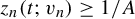 $z_n(t;v_n) \geq 1/A$
for sufficiently large n, contradicting Remark 3.5.
$z_n(t;v_n) \geq 1/A$
for sufficiently large n, contradicting Remark 3.5.
Finally, we prove Theorem 1.8.
Proof of Theorem 1.8
Let
 $p=0$
and define
$p=0$
and define ![]() , where
, where
 $r^{s/u}$
are the functions defined by (2.14). Since both functions
$r^{s/u}$
are the functions defined by (2.14). Since both functions
 $r^s$
and
$r^s$
and
 $r^u$
satisfy the Riccati equation (2.15), we get
$r^u$
satisfy the Riccati equation (2.15), we get
 $$ \begin{align*} \begin{aligned} \kappa_w &= w^2-V(\unicode{x3bb})w + \kappa_0 + Fw \\ &=\dfrac{(r^s)^2}{4}+\dfrac{(r^u)^2}{4}+\dfrac{r^s r^u}{2}-V(\unicode{x3bb})w + \kappa_0 + Fw\\ &=-\dfrac{(r^s)^2}{4}-\dfrac{(r^u)^2}{4}+\dfrac{r^s r^u }{2}\\ &=-\dfrac{1}{4}(r^s - r^u)^2. \end{aligned} \end{align*} $$
Since
 $r^s(v) \neq r^u(v)$
for all
$r^s(v) \neq r^u(v)$
for all
 $v\in SM$
by the transversality condition, it follows that
$v\in SM$
by the transversality condition, it follows that
 $\kappa _{w}< 0$
. In terms of regularity, the functions
$\kappa _{w}< 0$
. In terms of regularity, the functions
 $r^{s/u}$
are always smooth along the flow. However, thanks to Proposition 3.6, we also know that they are continuous since the Green bundles are transverse everywhere by assumption.
$r^{s/u}$
are always smooth along the flow. However, thanks to Proposition 3.6, we also know that they are continuous since the Green bundles are transverse everywhere by assumption.
This allows us to then prove our main result.
Proof of Theorem 1.6
Given the definitions of
 $E_s^*$
and
$E_s^*$
and
 $E_u^*$
in (1.13), we previously noted that
$E_u^*$
in (1.13), we previously noted that
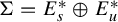 $\Sigma =E_s^*\oplus E_u^*$
. The estimates (1.12) then tell us that
$\Sigma =E_s^*\oplus E_u^*$
. The estimates (1.12) then tell us that
 $G^*_s=E_s^*$
and
$G^*_s=E_s^*$
and
 $G_u^*=E_u^*$
. By Theorem 1.8, we know that there exists a continuous function
$G_u^*=E_u^*$
. By Theorem 1.8, we know that there exists a continuous function
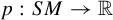 $p: SM\to {\mathbb {R}}$
, smooth along the flow, such that
$p: SM\to {\mathbb {R}}$
, smooth along the flow, such that
 $\kappa _p <0$
. We then apply [Reference Mettler and PaternainMP19, Theorem 3.7].
$\kappa _p <0$
. We then apply [Reference Mettler and PaternainMP19, Theorem 3.7].
4 Examples and counterexamples on the
$2$
-torus

The following system illustrates that when
 $V\unicode{x3bb} \neq 0$
, it is possible to have
$V\unicode{x3bb} \neq 0$
, it is possible to have
 $\mathbb {K}=0$
yet
$\mathbb {K}=0$
yet
 $G^*_{s}(v)\cap G^*_{u}(v)=\{0\}$
for some
$G^*_{s}(v)\cap G^*_{u}(v)=\{0\}$
for some
 $v\in SM$
. In particular, this shows that part (a) of Theorem 1.9 is optimal. Since
$v\in SM$
. In particular, this shows that part (a) of Theorem 1.9 is optimal. Since
 $S\mathbb {T}^2$
is a parallelizable manifold, each point
$S\mathbb {T}^2$
is a parallelizable manifold, each point
 $(x,v)\in S\mathbb {T}^2$
can be represented in coordinates
$(x,v)\in S\mathbb {T}^2$
can be represented in coordinates
 $(x,\theta )$
, where
$(x,\theta )$
, where
 $x\in [0,1)^2$
and
$x\in [0,1)^2$
and
 $\theta \in [0, 2\pi )$
is the angle such that
$\theta \in [0, 2\pi )$
is the angle such that
 $v=\cos (\theta ) \partial _{x_1}+\sin (\theta )\partial _{x_2}$
.
$v=\cos (\theta ) \partial _{x_1}+\sin (\theta )\partial _{x_2}$
.
Proposition 4.1. Let
 $(\mathbb {T}^2, g)$
be the
$(\mathbb {T}^2, g)$
be the
 $2$
-torus endowed with a flat Riemannian metric. Define
$2$
-torus endowed with a flat Riemannian metric. Define
 $\unicode{x3bb} \in \mathcal {C}^\infty (S\mathbb {T}^2, {\mathbb {R}})$
by
$\unicode{x3bb} \in \mathcal {C}^\infty (S\mathbb {T}^2, {\mathbb {R}})$
by ![]() . Then,
. Then,
 $\mathbb {K}=0$
and
$\mathbb {K}=0$
and
 $$ \begin{align*} \begin{aligned} &G^*_s(x,\pi/2)= {\mathbb{R}}(\psi_\unicode{x3bb} - \beta), \quad G^*_u(x,\pi/2)={\mathbb{R}}\psi_\unicode{x3bb},\\& G^*_s(x,-\pi/2)= {\mathbb{R}}\psi_\unicode{x3bb}, \ \ \ \qquad G^*_u(x,-\pi/2)= {\mathbb{R}}(\psi_\unicode{x3bb} - \beta). \\ \end{aligned} \end{align*} $$
Proof. Note that
 $(V\unicode{x3bb} )(x, \theta )=-\sin (\theta )$
. Unraveling the definitions, we get
$(V\unicode{x3bb} )(x, \theta )=-\sin (\theta )$
. Unraveling the definitions, we get
 $$ \begin{align*}\mathbb{K}=\pi^*K_g - H\unicode{x3bb} + \unicode{x3bb}^2+FV\unicode{x3bb} = \cos^2(\theta)-\cos^2(\theta)=0.\end{align*} $$
Observe that the two tori
 $$ \begin{align} \{(x,\theta)\in S\mathbb{T}^2\mid \theta=\pm \pi/2\} \end{align} $$
are flow-invariant. When
 $\theta = \pi /2$
, the solutions to (2.22) become
$\theta = \pi /2$
, the solutions to (2.22) become
 $$ \begin{align*}x(t)=e^{t}x(0), \quad y(t)=y(0)+x(0)(1-e^{t}).\end{align*} $$
Recall that we had set
 $p=V\unicode{x3bb} $
, so
$p=V\unicode{x3bb} $
, so
 $p(x, \pi /2)=-1$
. Further note that
$p(x, \pi /2)=-1$
. Further note that
 $m(t)=e^{t/2}$
. If we start with
$m(t)=e^{t/2}$
. If we start with
 $x(0)= 0$
and
$x(0)= 0$
and
 $y(0)\neq 0$
, which corresponds to a covector in
$y(0)\neq 0$
, which corresponds to a covector in
 ${\mathbb {R}}(\psi _\unicode{x3bb} -\beta )$
, we get that
${\mathbb {R}}(\psi _\unicode{x3bb} -\beta )$
, we get that
 $z(t)=y(0)e^{-t/2}$
is bounded for all
$z(t)=y(0)e^{-t/2}$
is bounded for all
 $t\geq 0$
. By Lemma 2.12, it follows that
$t\geq 0$
. By Lemma 2.12, it follows that
 $G^*_s(x, \pi /2)={\mathbb {R}}(\psi _\unicode{x3bb} -\beta )$
. However, if we start with
$G^*_s(x, \pi /2)={\mathbb {R}}(\psi _\unicode{x3bb} -\beta )$
. However, if we start with
 $x(0)\neq 0$
and
$x(0)\neq 0$
and
 $y(0)=-x(0)$
, which corresponds to a covector in
$y(0)=-x(0)$
, which corresponds to a covector in
 ${\mathbb {R}}\psi _\unicode{x3bb} $
, we get that
${\mathbb {R}}\psi _\unicode{x3bb} $
, we get that
 $z(t)=-x(0)e^{t/2}$
is bounded for all
$z(t)=-x(0)e^{t/2}$
is bounded for all
 $t\leq 0$
. By Lemma 2.12, it follows that
$t\leq 0$
. By Lemma 2.12, it follows that
 $G^*_u(x, \pi /2)={\mathbb {R}}\psi _\unicode{x3bb} $
.
$G^*_u(x, \pi /2)={\mathbb {R}}\psi _\unicode{x3bb} $
.
When
 $\theta =-\pi /2$
, we instead have
$\theta =-\pi /2$
, we instead have
 $$ \begin{align*}x(t)=e^{-t}x(0), \quad y(t)=y(0)+x(0)(e^{-t}-1), \quad m(t)=e^{-t/2},\end{align*} $$
so we can repeat the same arguments.
Remark 4.2. This example is also interesting from another perspective. In the classical paper [Reference Blallmann, Brin and BurnsBBB87], the authors construct a surface without conjugate points where the Green bundles are not continuous. They point out that the Green bundles are always continuous when
 $K_g \leq 0$
. Their example is quite elaborate, but it shares key features with the previous system: our two invariant tori (4.1) play the role of their closed geodesics
$K_g \leq 0$
. Their example is quite elaborate, but it shares key features with the previous system: our two invariant tori (4.1) play the role of their closed geodesics
 $\sigma _\pm $
. The advantage of our thermostat example is that it is much easier to understand and visualize (although it is not purely geodesic).
$\sigma _\pm $
. The advantage of our thermostat example is that it is much easier to understand and visualize (although it is not purely geodesic).
Illustration when
 $m=2$
.
$m=2$
.

To prove Theorem 1.4, we provide the following family of examples.
Lemma 4.3. Let g be a Riemannian metric on
 $\mathbb {T}^2$
and define
$\mathbb {T}^2$
and define
 $\unicode{x3bb} \in \mathcal {C}^\infty (S\mathbb {T}^2, {\mathbb {R}})$
by
$\unicode{x3bb} \in \mathcal {C}^\infty (S\mathbb {T}^2, {\mathbb {R}})$
by
where
 $h\in \mathcal {C}^\infty (\mathbb {T}^2, {\mathbb {R}})$
and m is an integer
$h\in \mathcal {C}^\infty (\mathbb {T}^2, {\mathbb {R}})$
and m is an integer
 $\geq 2$
. If
$\geq 2$
. If
 $$ \begin{align*}\Vert \partial h\Vert_{\infty}+h^2+(m-2)|h|<m-1-K_g,\end{align*} $$
then the thermostat
 $(\mathbb {T}^2, g, \unicode{x3bb} )$
has no conjugate points and it is projectively Anosov.
$(\mathbb {T}^2, g, \unicode{x3bb} )$
has no conjugate points and it is projectively Anosov.
Proof. Let ![]() , that is,
, that is,
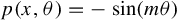 $p(x,\theta )=-\sin (m\theta )$
, and let us write
$p(x,\theta )=-\sin (m\theta )$
, and let us write ![]() . Then,
. Then,

Therefore, since
 $m\geq 2$
, we obtain the inequality
$m\geq 2$
, we obtain the inequality
The result follows from Theorem 1.1 and [Reference Mettler and PaternainMP19, Theorem 3.7].
By [Reference Plante and ThurstonPT72], we know that
 $S\mathbb {T}^2$
cannot admit an Anosov flow and, hence, this is an example of a projectively Anosov thermostat which is not Anosov. It is also easy to see that the non-wandering set is
$S\mathbb {T}^2$
cannot admit an Anosov flow and, hence, this is an example of a projectively Anosov thermostat which is not Anosov. It is also easy to see that the non-wandering set is
 $\Omega =\{(x, \theta )\in S\mathbb {T}^2\mid \cos (m\theta )=0, \, \sin (m\theta )=1\}$
. See Figure 4.
$\Omega =\{(x, \theta )\in S\mathbb {T}^2\mid \cos (m\theta )=0, \, \sin (m\theta )=1\}$
. See Figure 4.

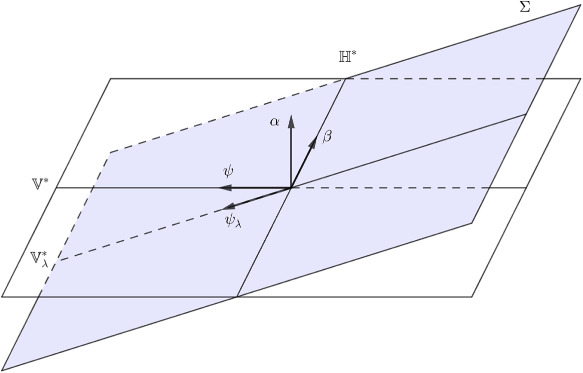


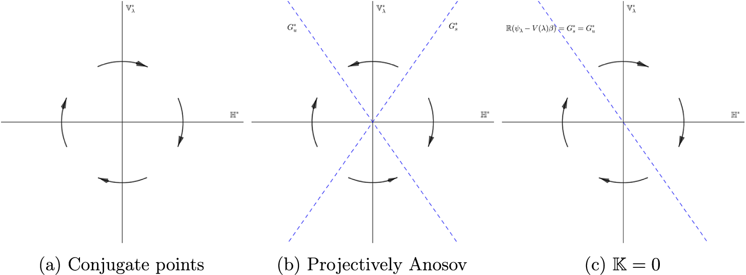

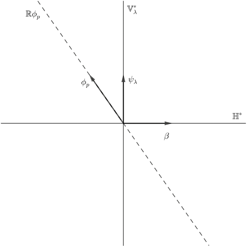


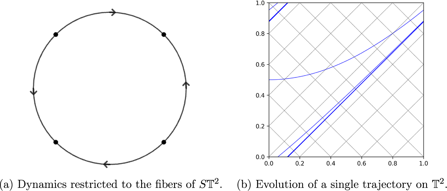


 Open access