


I. Introduction
Recent advancements in technology and the widespread use of online financial tools have transformed the way individuals interact with their finances. Today, almost all financial services are accessible through digital platforms, leading to a significant shift in how people manage their money.Footnote 1
When individuals access their online financial accounts, they can keep track of their account balances and review recent transactions, which allows them to assess their financial standing and plan their future spending. In this article, we test whether consumers are influenced by the way in which their personal finances are presented. Changes in the presentation of information can affect consumers’ sentiments, beliefs, or interpretation of the information and potentially lead to a change in behavior.
We conducted a field experiment on the users of an online account aggregation software. Account aggregation apps enable users to link various financial accounts, such as checking, savings, retirement, investment, mortgage, loans, and more, through a single application. This aggregation provides users with a comprehensive and real-time overview of their finances, including details such as net worth, total expenditures, expenditure breakdown by categories, and income.Footnote 2
Users of the app were provided with a personalized index that represents their net worth as a monthly cash flow. That is, instead of presenting net worth as a lump sum (e.g., $650,000), it was presented as the equivalent inflation-protected lifetime monthly cash flow, which depends on the user’s age and current market prices of life annuities (e.g., $2,000 per month for life). The index provides a relatively convenient reference for spending in comparison to the lump sum presentation, since consumers typically use monthly cash flows as a unit of measure for spending (e.g., rent, mortgage, utilities are typically billed monthly). We discuss the index in Section II.
Users of the app were randomly assigned to treatment groups that varied in the presentation of the index. The first variation in treatments was in the framing of the index. A significant body of research shows that consumers’ perceived value and attractiveness of life annuities depends on the frame used to describe them (Agnew, Anderson, Gerlach, and Szykman (Reference Agnew, Anderson, Gerlach and Szykman2008), Benartzi, Previtero, and Thaler (Reference Benartzi, Previtero and Thaler2011), Beshears, Choi, Laibson, Madrian, and Zeldes (Reference Beshears, Choi, Laibson, Madrian and Zeldes2014), Brown, Kling, Mullainathan, and Wrobel (Reference Brown, Kling, Mullainathan and Wrobel2008), (Reference Brown, Kling, Mullainathan and Wrobel2013), Brown, Kapteyn, and Mitchell (Reference Brown, Kapteyn and Mitchell2016), Goda, Manchester, and Sojourner (Reference Goda, Manchester and Sojourner2014), and Goedde-Menke, Lehmensiek-Starke, and Nolte (Reference Goedde-Menke, Lehmensiek-Starke and Nolte2014)).
Consumers place a higher value on annuities when the cash flow stream is described using a consumption frame (using words such as “spend” and “payment”) than when described using an investment frame (using words such as “invest” and “earnings”). The consumption frame prompts individuals to reflect on a negative scenario in which they have to cut their spending due to a lack of resources, leading them to place a higher value on lifetime monthly income. Fear appeal messages have been widely studied and shown to influence attitude, intentions, and behaviors effectively (Peters, Ruiter, and Kok (Reference Peters, Ruiter and Kok2013), Tannenbaum, Hepler, Zimmerman, Saul, Jacobs, Wilson, and Albarracín (Reference Tannenbaum, Hepler, Zimmerman, Saul, Jacobs, Wilson and Albarracín2015), and Witte (Reference Witte, Andersen and Guerrero1996)).
We test whether using the consumption frame to describe the index can also drive consumers to adjust their spending levels. Accordingly, we use two different labels as the name of the index:
Financial Sustainability Index (FSI): This label prompts users to think of the index as a reference to their spending activities. This name induces users to reflect on a scenario in which their financial condition is no longer “sustainable” and they are therefore forced to cut their spending.
Life Annuity Index (LAI): This label maintains a neutral tone and does not elicit any specific emotions from users. It simply describes the index for what it is—a life annuity quote.
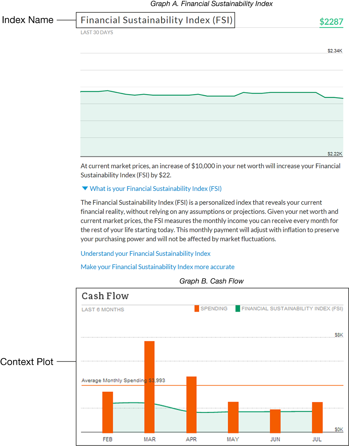
The second variation in the treatments is the salience of the comparison between the index and the user’s historical spending levels. Some of the treatment groups were presented with a time series plot that directly compares the index level with the user’s historical monthly spending (hereafter “context plot”; see Figure 1). Users in treatments that did not receive the context plot had access to the same information content. A time series plot of the index was presented on the dashboard page, and a separate time series plot of historical spending was available on the app’s Cash Flow page. However, without an explicit contrast between the index and spending, users are less likely to reflect on the difference between the two and adjust their spending.Footnote 3
Figure 1 shows the top of the dashboard page presented to users in the FSI-Plot treatment. The page displays the Financial Sustainability Index (FSI, Graph A)—a personalized measure of net worth expressed as an inflation-protected lifetime monthly cash flow—together with a statement linking changes in net worth to changes in the index. Graph A plots the FSI over the prior 30 days, and Graph B compares the user’s historical monthly spending over the prior 6 months (bars) with the FSI level (line), including a horizontal line for average monthly spending.

We find that users who were presented with the consumption frame (i.e., FSI) and a context plot decreased their discretionary spending by about 15% relative to users who received only the consumption frame with no plot or a context plot but with a neutral frame (i.e., LAI). The decrease in discretionary spending started immediately after the launch of the experiment and persisted throughout the 8 months in which the experiment materials were presented on the app. These consumers increased their spending levels only gradually after the removal of the experiment content and converged to the spending levels of consumers in unaffected groups after an additional 8 months.
The decrease in spending is most pronounced in relatively “tempting” spontaneous categories such as entertainment, restaurants, and clothing. This evidence is consistent with an improved ability to apply self-control due to an increased feeling of guilt and regret if they were to make the purchase (e.g., Hoch and Loewenstein (Reference Hoch and Loewenstein1991)). In contrast, we do not find a change in nondiscretionary spending such as gas, groceries, and utilities, which are difficult to adjust, especially over a short time period.
Furthermore, we find a decrease in infrequent large-ticket transactions. This evidence is consistent with Karlan, McConnell, Mullainathan, and Zinman (Reference Karlan, McConnell, Mullainathan and Zinman2016) and Sussman and Alter (Reference Sussman and Alter2012), showing that people tend to omit such “exceptional” transactions from their budget plan, and that salient reminders promote consumers to stay within their means.
Additionally, users in the affected treatments also decreased their cash withdrawals, representing an additional decrease in spending (i.e., not included in the discretionary spending variable). This decline in cash withdrawals is consistent with the notion that individuals assign a higher subjective value to cash transactions compared to noncash transactions, leading them to prioritize cutting back on cash transactions first (Raghubir and Srivastava (Reference Raghubir and Srivastava2008)).
Existing research on consumer spending has predominantly relied on either aggregate consumption data or low-frequency consumer-level data. However, recent studies have begun to leverage high-frequency transaction-level data, providing a more granular understanding of consumer behavior. This body of literature demonstrates that consumers exhibit strong spending habits, typically making gradual adjustments over an extended period in response to changes in economic factors like interest rates, income, or credit availability (Baker and Kueng (Reference Baker and Kueng2022), Havranek, Rusnak, and Sokolova (Reference Havranek, Rusnak and Sokolova2017), and Ravina (Reference Ravina2005)). This article shows that even in the presence of strong behavioral inertia, simple information design manipulations can prompt consumers to rapidly adjust their spending levels. Importantly, the response is caused by a change in consumers’ sentiment or a perceived change in financial well-being and not by a change in any economic variable.
Consumers in the affected groups decreased their spending immediately after receiving the experimental treatments. However, their spending increased only gradually after the experiment content was removed. This pattern aligns with findings from prior studies documenting a nonlinear adjustment in spending habits (Chen and Ludvigson (Reference Chen and Ludvigson2009), Ferson and Constantinides (Reference Ferson and Constantinides1991), and Ganong and Noel (Reference Ganong and Noel2019)). Specifically, these results are consistent with the predictions of the model proposed by Yogo (Reference Yogo2008), which incorporates habit formation into a reference-dependent utility function with loss aversion. According to the model, a negative shock elicits a larger response than a positive economic shock.
Framing effects have been extensively explored in the social sciences, demonstrating their influence across various domains.Footnote 4 However, framing information to specifically influence consumer spending poses unique challenges. First, it requires consumers to deviate from their established spending habits, which are typically resistant to change. Second, there is a temporal gap between the exposure to the experimental treatments and actual spending activity. Lastly, the treatments employed in our study do not prescribe a specific course of action, leaving consumers to decide if and how to adjust their spending. Nonetheless, this study demonstrates that through online financial apps, where consumers are frequently exposed to the treatments, certain information designs can indeed influence consumer spending.
Studies that examine framing effects on decision-making have often produced mixed results. Maheswaran and Meyers-Levy (Reference Maheswaran and Meyers-Levy1990) showed that issue involvement, which refers to the personal relevance and salience of an issue to an individual, is a key determinant of framing effects. They further demonstrated that negatively framed messages are more influential when they contain a high level of involvement. Kühberger (Reference Kühberger1998) conducted a meta-analysis of framing experiments and concluded that salience manipulations are critical determinants of framing effects. Consistent with this existing evidence, our study demonstrates that the fear appeal message incorporated in the consumption frame has an impact on spending behavior, but only when accompanied by a salient context. In other words, information must include both a relevant framing and a salient context for consumers to act upon it.
The article contributes to the extensive body of research on tools aimed at increasing consumers’ savings rates. Financial education programs have thus far proven to be costly and to have negligible effects on saving behavior (Campbell (Reference Campbell2006), Fernandes, Lynch, and Netemeyer (Reference Fernandes, Lynch and Netemeyer2014), and Willis (Reference Willis2011)). Tax subsidies for retirement accounts tend to benefit wealthier individuals, who are already better prepared for retirement (Chetty, Friedman, Leth-Petersen, Nielsen, and Olsen (Reference Chetty, Friedman, Leth-Petersen, Nielsen and Olsen2014)). Employers’ matching contributions to retirement accounts have had limited success in increasing saving rates (Choi, Laibson, Madrian, and Metrick (Reference Choi, Laibson, Madrian and Metrick2002), Choi, Laibson, and Madrian (Reference Choi, Laibson and Madrian2011), and Duflo, Gale, Liebman, Orszag, and Saez (Reference Duflo, Gale, Liebman, Orszag and Saez2006)). Behavioral tools such as choice architecture, reminders, and information design have repeatedly been proven to be powerful in influencing savings and retirement account contributions (Bai, Chi, Liu, Tang, and Xu (Reference Bai, Chi, Liu, Tang and Xu2021), Chetty et al. (Reference Chetty, Friedman, Leth-Petersen, Nielsen and Olsen2014), Choi et al. (Reference Choi, Laibson, Madrian and Metrick2002), Choi, Laibson, Madrian, and Metrick (Reference Choi, Laibson, Madrian, Metrick and Wise2004), Karlan et al. (Reference Karlan, McConnell, Mullainathan and Zinman2016), Madrian and Shea (Reference Madrian and Shea2001), and Thaler and Benartzi (Reference Thaler and Benartzi2004)). However, these behavioral tools may not be applicable to a significant portion of nonretired households that have no access to retirement accounts.Footnote 5 In addition, the effect of an increase in retirement contributions on the overall saving rate is mitigated by early withdrawal from these accounts (Argento, Bryant, and Sabelhaus (Reference Argento, Bryant and Sabelhaus2015), Beshears, Choi, Clayton, Harris, Laibson, and Madrian (Reference Beshears, Choi, Clayton, Harris, Laibson and Madrian2025), and Beshears, Choi, Iwry, John, Laibson, and Madrian (Reference Beshears, Choi, Iwry, John, Laibson and Madrian2020)) and an increase in borrowing activity (Beshears, Choi, Laibson, Madrian, and Goda (Reference Beshears, Choi, Laibson and Madrian2011)). This article shows that information design can influence spending, which is the flip side of savings. Given the wide use of online financial services, information design tools can be easily implemented and distributed to a large mass of consumers at a low cost, including lower-income individuals who have no retirement accounts.Footnote 6
II. Personalized Index
Account aggregation apps typically present the users’ net worth as the first item on the first page users visit after logging in. In this study, all treatment groups received a personalized index that presented their net worth, but with a change in the unit of measure. Instead of presenting net worth as a lump sum, it was presented as the equivalent inflation-protected lifetime monthly cash flow, which depends on the user’s age, state of residence, and current market prices. This index reflects the market quote of a monthly cash flow from an immediate, inflation-protected life annuity. Life annuities are sold by large financial institutions (typically insurance companies) and provide a hedge for market, longevity, and inflation risks. By using the market prices and current net worth of the user (instead of a projected future net worth), the index does not require any assumptions.
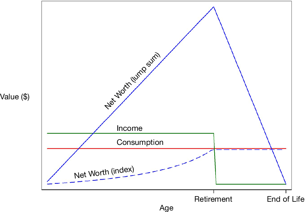
Figure 2 illustrates the index dynamics in comparison to net worth as a lump sum in a simplified life cycle model with no uncertainty. An individual with a known end-of-life date receives a constant income flow every period until a known retirement age. Under any standard preferences, the individual will perfectly smooth their consumption over their lifetime. Net worth as a lump sum increases during the consumer’s working years, peaks at retirement age, decreases over the retirement years, and depletes at the end of life. Net worth as a personalized index describes the constant cash flow level that the consumer can generate for the rest of their life, given their current net worth and time till the end of life. During the consumer’s working years, like the lump sum, the index gradually increases. Two factors contribute to the rate of increase: wealth accumulation and the shortening of remaining life. The index peaks at retirement age, where it converges to the consumption level and remains constant until the end of life.
Figure 2 illustrates the index and net worth level of a life cycle of a consumer with a constant income level during their working years and no income after retirement. Given no uncertainty, the consumer can smooth their consumption perfectly. Net worth as a lump sum is the accumulated wealth from income and savings. Net worth as an index is the constant consumption level that the person can afford until the end of their life, given their level of accumulated wealth and time till the end of life. For simplicity, the real return on savings is set to zero. The plot of Net Worth as a lump sum is scaled down by a factor of 6.

This index can potentially provide useful financial guidance for the individual. For a person in retirement, the index accurately shows the optimal level of consumption in the simplified framework described above. A person approaching retirement age can check whether the consumption level is close to the index level. If the difference between spending and the index levels is large, they can consider adjusting the consumption level, the income, or even the retirement age. For a younger person, the index is significantly lower than the optimal consumption level. That person can monitor whether the index level and the consumption level converge quickly enough.
The presentation of the personalized index can impact consumers’ behavior through several nonexclusive channels. First, the index might reduce consumers’ “illusion of wealth.” Goldstein, Hershfield, and Benartzi (Reference Goldstein, Hershfield and Benartzi2016) show that, when net worth is sufficiently high, people tend to perceive it as having a higher value than the equivalent monthly cash flow. The presentation of net worth as a monthly cash flow instead of a lump sum might encourage users to feel less wealthy and change their spending behavior.
Second, monthly cash flow is the commonly used unit of measure for spending, such as monthly bills for rent, mortgage, and utilities. The presentation of net worth as a monthly cash flow provides a reference point for spending activity that encourages consumers to mentally simulate their lives under a different monthly budget. Reference-dependent utility consumers are predicted to be especially sensitive to potential changes in their standard of living and might therefore adjust their spending levels.
Third, the index might serve as an anchor for spending activity. Anchor effects occur when an initial salient value influences individuals’ subsequent estimations or decisions. These effects are especially pronounced when there are no other competing reference points or information available (Kahneman (Reference Kahneman1992)). Given that consumers typically do not know their optimal level of spending, nor does the app provide any other benchmark for spending, the index might have a strong impact as an anchor.
Note that none of these channels requires consumers to fully understand the economic interpretation of the index. In fact, it is highly plausible that many users do not fully grasp its meaning, since doing so would require relatively advanced financial and economic knowledge.
There are several reasons for using the index as the subject for information design manipulations. First, it is new information content that is not already available on the app. This requirement ensures that all users have the same level of familiarity with the experimental content and are not biased toward the old information design. Second, the selection of the index is motivated by previous studies in behavioral economics, policy discussions, and practices in the financial industry. The academic research discussed in Section I examines the effects of information design manipulation on consumers’ demand for life annuities, providing a foundation for exploring the impact of the personalized index on consumer spending in this study. Additionally, the recent SECUREwhite_Act (2019) requiring retirement account providers to display the account’s worth as a projected lifetime monthly income and the offering of similar personalized indices by the financial industry, such as “CoRI” by BlackRock, demonstrate the applicability of the index to consumers’ spending and savings decisions.
III. Experimental Design
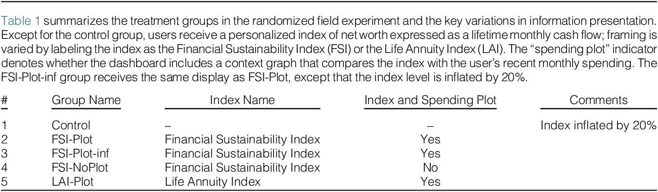
The experiment was embedded in a financial management app that is offered to the general public at no cost. The first web page users view after logging into the app is the “dashboard” page, which provides a brief summary of the user’s finances. The pre-experiment dashboard page is presented in Figure C1 in the Supplementary Material. Users were randomly assigned to seven groups.Footnote 7 Apart from the control group, all treated groups received a personalized index. The treatments differed in the name of the index and in the availability of a context plot. The treatments are summarized in Table 1 and illustrated in Figure 1. The treatment groups are defined as follows:

Control Group (Figure C1 in the Supplementary Material): The dashboard page was not changed for users in this group. The page includes time-series plots of net worth, total income, and total spending. This group serves as a baseline to detect any changes in financial activity that are not related to the experiment.
FSI-Plot Group (Figures C2 and C3 in the Supplementary Material): Users received the Financial Sustainability Index, which contains a fear appeal message. They also received a context plot providing a salient comparison between the index level and historical monthly spending.
FSI-Plot-inf Group: Several studies have suggested that high annuity prices might explain the low demand for life annuities.Footnote 8 If annuities are overpriced, the consumers might respond to the index because it quotes an overly pessimistic cash flow. To address this concern, this group received the same treatment as the FSI-Plot group, except the quoted index was inflated by 20%. A differential response between these two groups would indicate that the change in behavior is sensitive to the exact quote used.
FSI-NoPlot Group (Figure C4 in the Supplementary Material): Users received the FSI and no context plot. By comparing the behavior of this group to that of users in the FSI-Plot group, we can identify the impact of providing a salient comparison between the index and spending.
LAI-Plot Group (Figure C5 in the Supplementary Material): Users received the Life Annuity Index and no context plot. By comparing the behavior of this group to that of users in the FSI-Plot group, we can identify the impact of the framing effect embedded in the index names.
The experiment did not include a treatment that presents the index using neutral framing (LAI) with a context plot due to the limited number of users available for the experiment. As a result, we only test the impact of the context plot in the presence of consumption framing.
Goldstein et al. (Reference Goldstein, Hershfield and Benartzi2016) and Goda et al. (Reference Goda, Manchester and Sojourner2014) showed that individuals respond to information about changes in their cash flow stream. Following their findings, users received information about the sensitivity of the index level to changes in their net worth (“At current market prices, an increase of $10,000 in your net worth will increase your [FSI/LAI] by $[X]”).
The dashboard page of all the treated groups included a link to an FAQ page. The FAQ for each group was adjusted to reflect the corresponding index name. The FAQ page for the FSI-Plot group is presented in Figures C8 and C9 in the Supplementary Material.
Historical monthly income was removed from the dashboard page in all treatments, but was available to all users on the Cash Flow page of the app. Kahneman (Reference Kahneman1992) shows that anchor effects are especially pronounced when no other competing reference points or information is available. The removal of monthly income from the landing page decreases the salience of this information and potentially increases the likelihood of using the index as the new benchmark for spending. In addition, historical monthly spending was not presented on the dashboard page for treatments that did not receive a context plot. All users could view their historical spending on the Cash Flow page of the app. The removal of monthly spending from the landing page reduces the salience of this information and the ability of users to directly compare it to the index level.
IV. Data
A. Annuity Price Quotes
We obtain life annuity prices from Hueler’s Income Solutions® annuity quoting platform. This platform allows individuals to receive customized quotes of identical annuity contracts from large insurance companies in real time. All insurance companies that provide quotes are rated “A” or above by Moody’s, S&P, and A.M. Best. The costs of investment management, distribution, administration, and other costs associated with annuity products are reflected in the annuity quotes. We use annuity quotes of inflation-protected life annuities for single, male buyers (reflecting the majority of the app users) with a nonqualified income of $100,000. We obtain the full annuity quotes grid for all ages between 35 and 85, all commencement dates between immediate and the age of 85, and all states.Footnote 9 Annuity quotes were updated once a week during the experiment. The personal index for each user was calculated as the average quote from all companies given the user’s age, state of residence, and net worth.
B. Consumer Data
The sample consists of users of the financial management app who are not clients or prospective clients of the app provider’s wealth management services. We restrict the sample to users above the age of 35, which is the minimum age of life annuity quotes. Additionally, retired users are excluded from the sample to accommodate the two treatment groups, where the index represents a deferred annuity quote with a commencement date at retirement. We keep users who had been using the app for at least 5 months before the experiment.
The sample includes only users who logged into the app at least once in the 3 months before the experiment, linked at least one credit or debit account, and had an average monthly income and spending above $1,000 in the 5 months before the experiment launch. These restrictions ensure that the sample includes only users who are actively using the app. We also exclude users with a net worth below $5,000 so that the level of the personal index is sufficiently positive.
Users of mobile financial apps log in to view their accounts more frequently than users who log in only from personal computers (Carlin, Olafsson, and Pagel (Reference Carlin, Olafsson and Pagel2023)). To ensure consistency in the level of exposure to the app and the experiment material, we include only users who have installed the mobile app prior to the start of the experiment and have logged in using a mobile device at least once in the 3 months before the experiment launch.
The final sample consists of 3,138 users. Data on users’ transactions and login activity are collected for a period of 25 months, starting 5 months before the experiment launch and continuing for 20 months after.
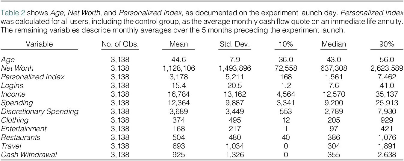
Table 2 presents summary statistics of the sample as documented on Mar. 17, 2014, the launch day of the experiment. The average age in the sample is 45. The average net worth is $1.1 million (median $0.6 million), and the average monthly income from all sources is $16.7K (median $12.6K). The personalized index in this table was calculated for all users, including the control group, as the average quote on an immediate inflation-protected life annuity. The average index level is $3,175, and the median is $1,561. The average number of monthly logins during the 5 months before the experiment’s launch is 15.4 (median of 7.6), indicating that users in the sample are actively using the app. The average monthly spending is about $12K, and the median is $9.2K. The spending levels of users in this sample are well above their personalized index levels, as predicted for consumers relatively far from retirement age (see discussion in Section II and Figure 2).

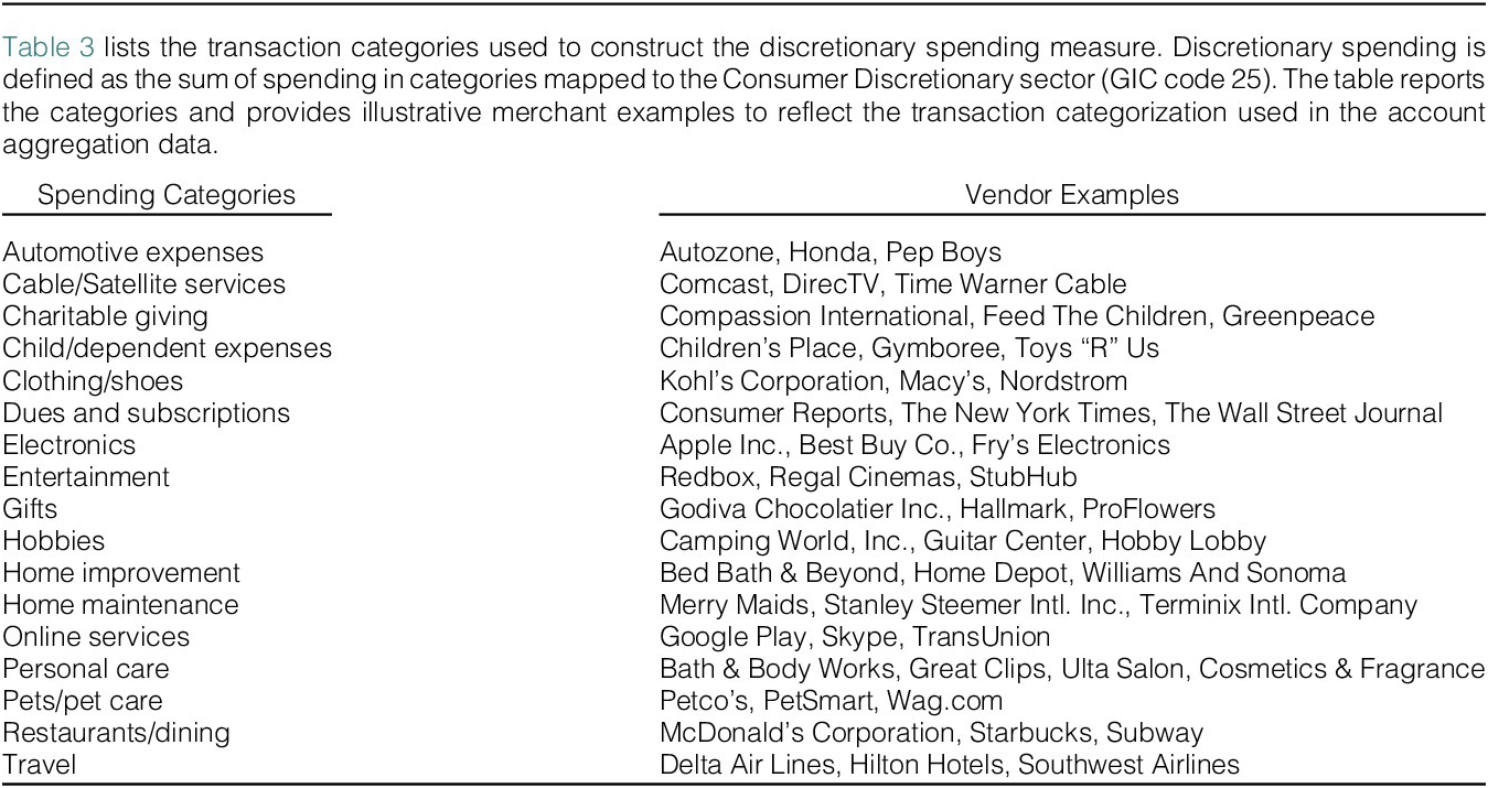
The main variable of interest is discretionary spending, which refers to spending on items over which consumers have relatively more control and can adjust over a short period, such as entertainment and restaurants. We define discretionary spending as the sum of spending in categories that correspond to industries in the Consumer Discretionary sector according to the Global Industry Classification Standard (GIC code 25). The complete list of categories with example vendors for each category is presented in Table 3. The average level of discretionary spending in this sample is $3,689 (median $2,789), constituting about 30% of overall spending. We analyze expenditures on clothing, entertainment, restaurants, and travel, which are relatively large components of discretionary spending. We also analyze cash withdrawals, which reflect additional spending not included in the discretionary spending variable. The average monthly cash withdrawal in this sample is $925, and the median is $355.

Overall, the consumers in this sample are relatively wealthy and are similar to consumers in the 80th percentile of the income distribution based on their income level, overall spending, and spending on the categories studied in this article.Footnote 10
V. Empirical Specification
Experiment materials were available on the app for a period of 8 months. The data cover the period from $ t=-5 $
to
$ t=-5 $
to $ t=19 $
, where the experiment launch month is
$ t=19 $
, where the experiment launch month is $ t=0 $
. We define two indicator variables:
$ t=0 $
. We define two indicator variables: $ Intra $
: equals 1 for event months in which experiment material was presented on the app, from
$ Intra $
: equals 1 for event months in which experiment material was presented on the app, from $ t=0 $
to
$ t=0 $
to $ t=7 $
.
$ t=7 $
. $ Post $
: equals 1 for event months after the removal of experimental material from the app, from
$ Post $
: equals 1 for event months after the removal of experimental material from the app, from $ t=8 $
to
$ t=8 $
to $ t=19 $
.
$ t=19 $
.
The main empirical specification is
 $$ {y}_{i,t}=\sum \limits_{j=2}^{j=5}{\beta}_j{TG}_{j,i}{Intra}_t+\sum \limits_{j=2}^{j=5}{\gamma}_j{TG}_{j,i}{Post}_t+{\delta}_i+{\theta}_j+{\epsilon}_{i,t}, $$
where $ {y}_{(i,t)} $
is an outcome variable such as logins or log spending for consumer
$ {y}_{(i,t)} $
is an outcome variable such as logins or log spending for consumer $ i $
in event month
$ i $
in event month $ t $
.
$ t $
. $ {TG}_j $
are treatment group indicator variables for each of the groups, where the omitted group serves as the reference level.
$ {TG}_j $
are treatment group indicator variables for each of the groups, where the omitted group serves as the reference level. $ {\delta}_i $
is an individual fixed effect, and
$ {\delta}_i $
is an individual fixed effect, and $ {\theta}_j $
is an event-month fixed effect. Standard errors are clustered at the consumer level.Footnote
11
$ {\theta}_j $
is an event-month fixed effect. Standard errors are clustered at the consumer level.Footnote
11 $ {\beta}_j $
captures the average change in the outcome variable between the pre-experiment months (
$ {\beta}_j $
captures the average change in the outcome variable between the pre-experiment months ( $ t=-5 $
to
$ t=-5 $
to $ t=-1 $
) and the experiment months (
$ t=-1 $
) and the experiment months ( $ t=0 $
to
$ t=0 $
to $ t=7 $
) of consumers in the treatment group
$ t=7 $
) of consumers in the treatment group $ j $
, relative to the same change in the omitted treatment group. Similarly,
$ j $
, relative to the same change in the omitted treatment group. Similarly, $ {\gamma}_j $
captures the average change in the outcome variable between the pre-experiment months (
$ {\gamma}_j $
captures the average change in the outcome variable between the pre-experiment months ( $ t=-5 $
to
$ t=-5 $
to $ t=-1 $
) and the post-experiment months (
$ t=-1 $
) and the post-experiment months ( $ t=8 $
to
$ t=8 $
to $ t=19 $
) of consumers in the treatment group
$ t=19 $
) of consumers in the treatment group $ j $
, relative to the same change in the omitted treatment group.
$ j $
, relative to the same change in the omitted treatment group.
In addition, we estimate the following specification for each of the treatment groups separately:
 $$ {y}_{i,t}=\sum \limits_{t=-4}^{t=19}{\beta}_tI(t)+{\delta}_i+{\epsilon}_{i,t}, $$
where $ I(t) $
is an event-month indicator for month
$ I(t) $
is an event-month indicator for month $ t $
.
$ t $
. $ {\beta}_t $
captures the change in the outcome variable in event month
$ {\beta}_t $
captures the change in the outcome variable in event month $ t $
relative to event month
$ t $
relative to event month $ t=-5 $
. This within-group time-series analysis allows us to test the speed and duration of consumers’ response to the treatments.
$ t=-5 $
. This within-group time-series analysis allows us to test the speed and duration of consumers’ response to the treatments.
VI. Results
A. Attention
The experiment content was presented at the top of the dashboard page, which is the first page users see after logging into the app. Given this placement of the experiment content, login activity measures users’ exposure to the experiment materials and level of attention to their personal finances.
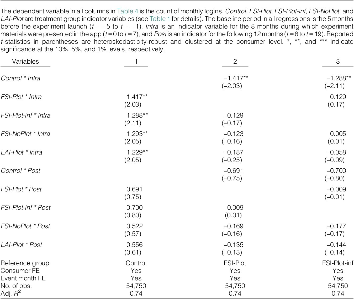
Table 4 reports the effect of the treatments on the users’ number of logins per month. The reference treatment group in the first column is the control group. The coefficients of all the interaction variables between the treatment indicators and $ Intra $
reveal that the change in monthly logins between the pre-experiment months and the experiment months is significantly larger for all the treatment groups relative to the same change in the control group. Users in each of the treatment groups increased their login frequency during the experiment months by about 1.3 logins per month relative to the control group. The coefficients of the interaction variables between the treatment indicators and
$ Intra $
reveal that the change in monthly logins between the pre-experiment months and the experiment months is significantly larger for all the treatment groups relative to the same change in the control group. Users in each of the treatment groups increased their login frequency during the experiment months by about 1.3 logins per month relative to the control group. The coefficients of the interaction variables between the treatment indicators and $ Post $
show that after the removal of the experiment material, the change in login frequency of users in all treatment groups relative to the pre-experiment months is still greater than the same change in the control group (about 0.6 more monthly logins), but the difference is not statistically significant. Columns 2 and 3 repeat the same regression with the FSI-Plot and FSI-Plot-inf groups as the baseline treatments. Although all groups increased their attention level during the experiment months relative to the control group, there are no notable differences in the login frequency across any of the other treatment groups during or after the experiment.
$ Post $
show that after the removal of the experiment material, the change in login frequency of users in all treatment groups relative to the pre-experiment months is still greater than the same change in the control group (about 0.6 more monthly logins), but the difference is not statistically significant. Columns 2 and 3 repeat the same regression with the FSI-Plot and FSI-Plot-inf groups as the baseline treatments. Although all groups increased their attention level during the experiment months relative to the control group, there are no notable differences in the login frequency across any of the other treatment groups during or after the experiment.

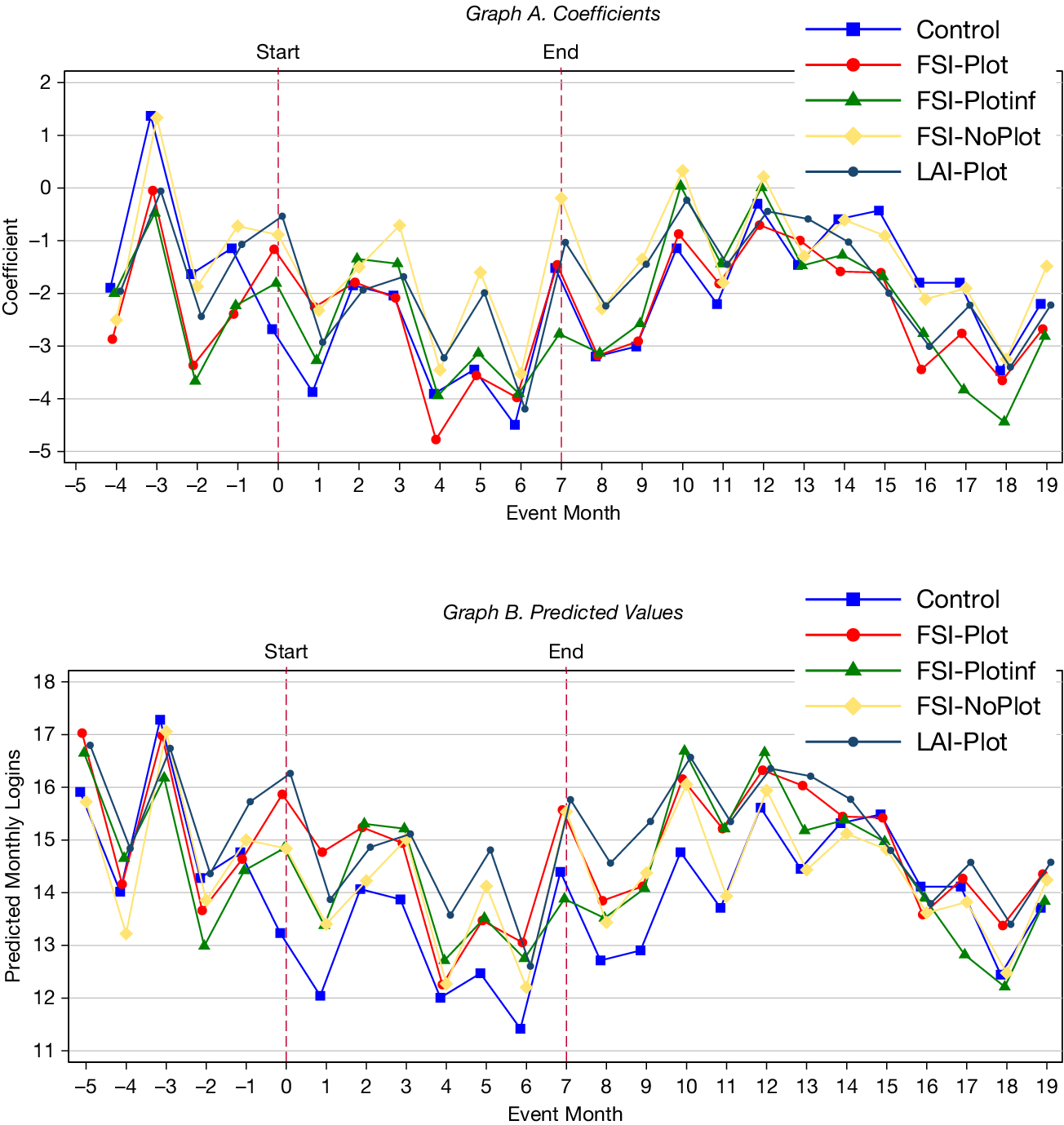
The results for the time series analysis for each of the treatment groups are presented in Figure 3 (formal results are in Table 1). Graph A displays the estimated coefficients in Equation (2), and Graph B shows the average predicted values in each event month. The monthly login frequency of the treatment groups is similar and highly correlated between all the groups before the start of the experiment. At $ t=0 $
, all the treated groups immediately diverge from the control group, and the predicted login frequency remains higher throughout the experiment months. The change in the login frequency of all the treated groups is still higher than that of the control group for about 3 months after the experiment, after which all the groups converge to the same login frequency.
$ t=0 $
, all the treated groups immediately diverge from the control group, and the predicted login frequency remains higher throughout the experiment months. The change in the login frequency of all the treated groups is still higher than that of the control group for about 3 months after the experiment, after which all the groups converge to the same login frequency.
Graph A of Figure 3 shows the estimated coefficients in a regression of monthly login count on event month indicator variables with consumer fixed effects for each treatment group. Graph B shows the average predicted values for that regression. Detailed regression results are in Table 1.

Overall, the login analysis shows that users in all treated groups increased the level of attention to their finances throughout the experiment months. The change in login frequency is significant but small in magnitude, with only slightly more than one login per month relative to the control group. The change in login frequency started immediately after the launch of the experiment and can be attributed to interest in the new content on the app. The lack of difference in login frequency across the treated groups reveals that the increased attention cannot be attributed to any specific treatment feature, such as the index name or the presentation of a context plot. Therefore, any differences in spending behavior across the different treatments cannot be attributed to a difference in consumers’ login frequency.
B. Discretionary Spending
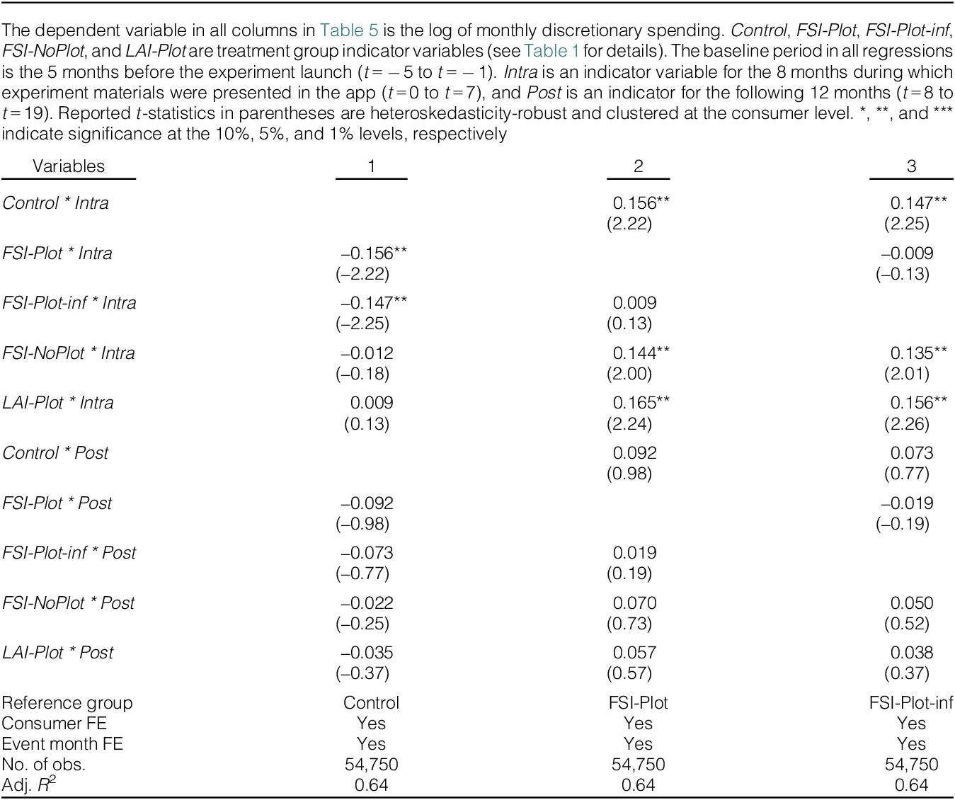
Table 5 presents the analysis of the treatment effects on the log of discretionary spending. The first column shows that both the FSI-Plot and the FSI-Plot-inf reduced their discretionary spending during the experiment period by about 15% relative to the change in the control group over the same period. None of the other groups had a significant change in their spending behavior. Columns 2 and 3 formally show that there were no significant differences between the FSI-Plot and the FSI-Plot-inf groups, and that the change in discretionary spending of these groups is significantly lower than that of the FSI-NoPlot and the LAI-Plot groups. Using the sample mean of monthly discretionary spending ($3,689), a 15% decline in discretionary spending corresponds to a drop of $553 per month, which is about 4.5% of overall monthly spending. The coefficients of the interaction variable between the treatment indicators and $ Post $
show that after the removal of the experiment material from the app, there were no significant differences in discretionary spending between any of the groups.
$ Post $
show that after the removal of the experiment material from the app, there were no significant differences in discretionary spending between any of the groups.

This analysis confirms that information design can have a substantial impact on consumers’ discretionary spending. However, the effect is sensitive to specific features in information presentation. Consumers only respond when the index is presented both under the consumption frame and contains a salient context. Presentation of either the consumption frame or a salient context by itself does not yield a partial response. The lack of difference in effect size between the FSI-Plot and FSI-Plot-inf groups indicates that the effect is robust to the exact quote used in the index.
Treatments that did not receive a context plot with a consumption framing of the index name did not show any differences in spending relative to the control group, suggesting that the omission of monthly income and spending from the dashboard page did not impact users’ spending behavior. However, the decrease in spending in the FSI-Plot and the PSI-Plot-inf groups might have been smaller in magnitude if income was still presented on the dashboard page, providing a salient alternative benchmark for spending instead of the index.
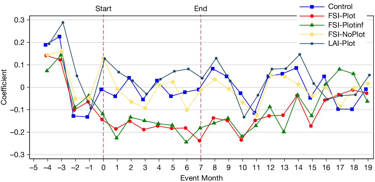
Figure 4 shows the dynamics of the change in discretionary spending for each of the experiment groups relative to their spending at $ t=-5 $
(formal results are in Table 3). The changes in discretionary spending of all the groups are positively correlated and similar in magnitude before the experiment launch. The peak in discretionary spending at
$ t=-5 $
(formal results are in Table 3). The changes in discretionary spending of all the groups are positively correlated and similar in magnitude before the experiment launch. The peak in discretionary spending at $ t=-3 $
and the sharp decline at
$ t=-3 $
and the sharp decline at $ t=-2 $
are driven by seasonal effects, with a high spending month in December followed by a low spending month in January. The change in discretionary spending of the FSI-Plot and FSI-Plot-inf groups diverges from all the other groups immediately at the launch of the experiment and remains lower throughout the experiment. The gap between these two groups and all the other groups remained large for three additional months after the experiment and gradually decreased afterward. The changes in discretionary spending of all the groups converge only at
$ t=-2 $
are driven by seasonal effects, with a high spending month in December followed by a low spending month in January. The change in discretionary spending of the FSI-Plot and FSI-Plot-inf groups diverges from all the other groups immediately at the launch of the experiment and remains lower throughout the experiment. The gap between these two groups and all the other groups remained large for three additional months after the experiment and gradually decreased afterward. The changes in discretionary spending of all the groups converge only at $ t=16 $
, 9 months after the removal of the experimental content from the app.
$ t=16 $
, 9 months after the removal of the experimental content from the app.

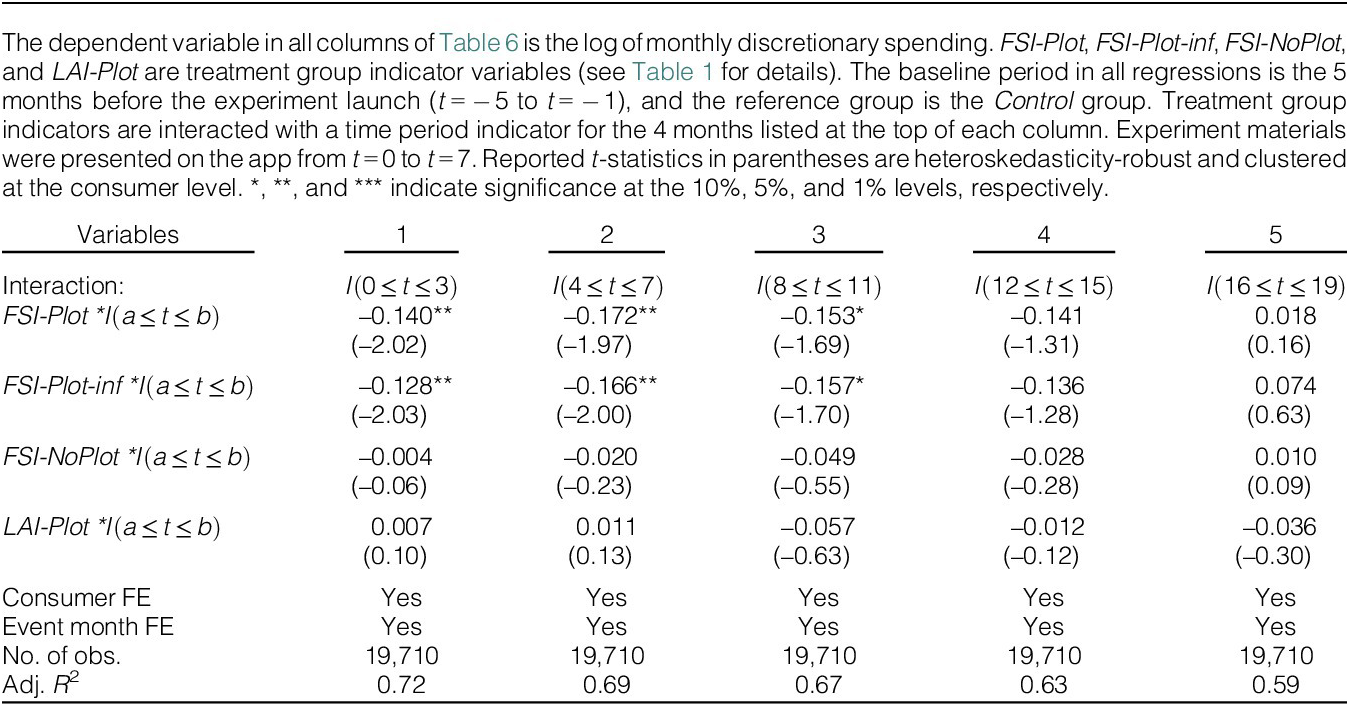
The analysis in Figure 4 shows the within-group evolution of discretionary spending. To test the persistence of the effect after the experiment duration across groups, we conduct an additional analysis of discretionary spending over shorter periods than used in Equation (1). The results of this analysis are presented in Table 6. The dependent variable is the log of discretionary spending. The explanatory variables are the interactions of group indicators and a time period indicator where the time period in each regression is listed at the top of the column. The control group is the baseline group in all columns, and the reference time period is the 5 months before the experiment launch.Footnote
12 The first two columns show that the average change in discretionary spending is about 15% lower than the change in the control group during the experiment months. Column 3 shows that the decline in discretionary spending of the affected treatments during the following 4 months remained about 15% lower than the change in the control group. However, this effect is only significant at the 10% level. The magnitude of the change in these groups decays over time, and the point estimates of all the groups are similar to each other between $ t=16 $
and
$ t=16 $
and $ t=19 $
.
$ t=19 $
.

Overall, the analysis in Figure 4 and Table 6 shows that the treatments had lasting effects beyond the period in which the experiment content was presented on the app. The FSI-Plot and FSI-Plot-inf treatment groups reduced their discretionary spending immediately at the start of the experiment, but resumed their nontreatment levels of spending only after several months.
C. Spending Categories
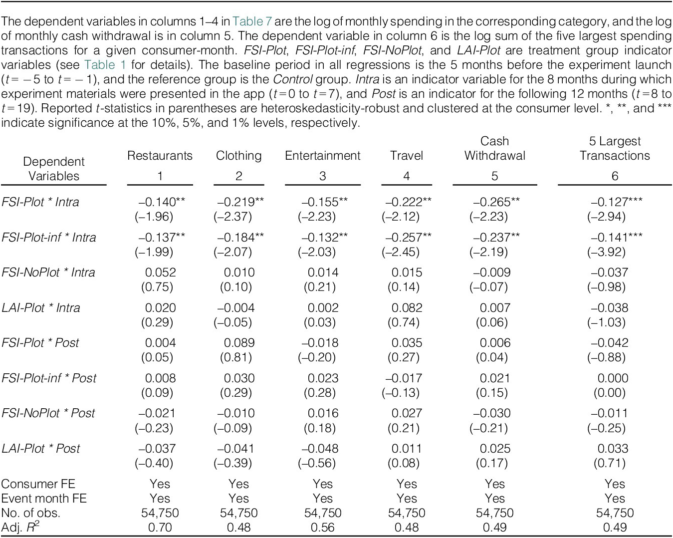
In Table 7, we test the average spending response in different spending categories. Column 1 shows that both the FSI-Plot and FSI-Plot-inf reduced their restaurant expenditures by about 14% relative to all the other groups during the experiment months. Restaurant spending is relatively easy to adjust by visiting less expensive restaurants or dining at home. Users in these groups also reduced their clothing expenditures by a significant 20% relative to the other groups (column 2). Clothing expenses can be relatively easily adjusted as well by reducing purchase frequency or clothing price. Column 3 shows that users in the FSI-Plot and FSI-Plot-inf treatments decreased their expenditures on entertainment by about 14% relative to the change in other groups. Column 4 shows a decrease of about 24% in travel expenses for users in these two groups. Travel is likely to be a luxury item for many consumers that can be adjusted by choosing a more modest vacation or skipping it altogether.

Column 5 shows that consumers in the FSI-Plot and FSI-Plot-inf groups reduced their cash withdrawals by about 25% compared to other groups. Unlike the previous spending categories, cash withdrawals are not included in the discretionary spending variable. Therefore, this decrease in cash withdrawals reflects an additional decrease in spending. This evidence is consistent with consumers placing a higher subjective value on cash transactions and therefore being more likely to reduce these transactions first (Raghubir and Srivastava (Reference Raghubir and Srivastava2008)).
Sussman and Alter (Reference Sussman and Alter2012) classified transactions into ordinary (i.e., common and frequent) transactions and exceptional (i.e., unusual or infrequent) transactions, with many of the largest expenses being the most exceptional.Footnote 13 They show that although consumers are fairly skillful at planning their ordinary spending, they systematically underestimate their future expenditures on exceptional items. Consumers tend to categorize each exceptional expense as a unique occurrence and consequently overspend after a series of exceptional expenses. Moreover, changes in large and infrequent expenditures might be easier to implement, as the consumer will have to make a single (large) mental effort to apply self-control rather than exercise discipline and sacrifice every day.
We test if the decrease in spending is a result of a reduction in spending on exceptional expenses. We use the sum of the five largest transactions of each user in a given month as a proxy for large and infrequent transactions.Footnote 14 Note that the consumers’ largest transactions are typically rent, mortgage, and loan payments. However, these expenses are typically constant over time and are therefore absorbed by the consumer fixed effects. Column 6 shows that both the FSI-Plot and FSI-Plot-inf groups significantly reduced their large transactions during the experiment months, suggesting that these users avoided or reduced spending on infrequent large-ticket transactions. Overall, the reduction in spending is driven by a decrease in both common and exceptional transactions.
D. Additional Tests
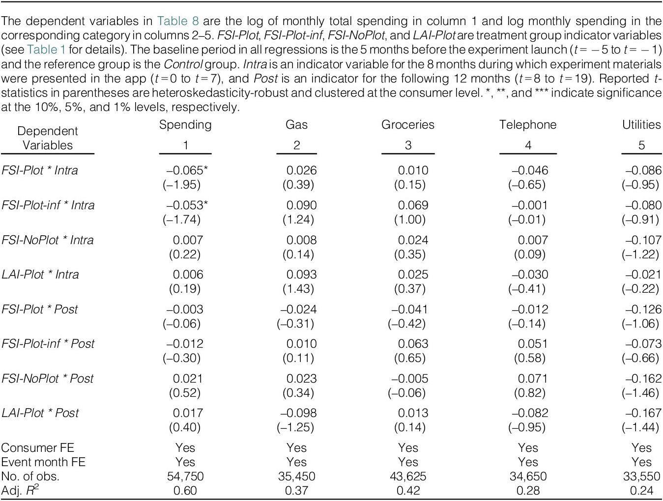
In the first column of Table 8, we test the effect of the different treatments on the users’ overall spending level. We find a decline of about 6% in overall spending in the FSI-Plot and FSI-Plot-inf groups relative to the change in any of the other treatment groups. However, this decline is only significant at the 10% level. Given the average monthly mean of overall spending of $12,364, a decrease of 6% in overall spending translates to a reduction of approximately $742 per month. This decrease roughly corresponds to the combined decrease in monthly discretionary spending and cash withdrawals.Footnote 15 In addition, we test the effect of the different treatments on overall monthly spending minus discretionary spending and cash withdrawals, and find no significant differences between any of the groups. This evidence confirms that consumers did in fact decrease their spending levels and did not shift their expenses from discretionary spending and cash transactions to other spending categories.

As a falsification test, we check if there is a change in spending categories that are relatively difficult to adjust, especially in the short run. We find no significant differences in spending on gas, groceries, telephone, or utilities between any of the treatment groups (columns 2–5).
VII. Conclusion
This article documents the critical impact of information design on consumers’ spending behavior. The frame in which the information is presented and the salience of the context can have a significant impact on consumers’ spending, despite strong behavioral inertia in spending and the temporal distance between exposure to treatment and the spending activity. Furthermore, the effects on spending behavior start immediately after the exposure to the treatment and last for several months beyond the experiment duration, showing that the impact of the information design lasts beyond the exposure to the treatment and supports an asymmetrical adjustment of spending habits.
Information tools that influence spending behavior offer several advantages over the existing tools aimed at influencing saving behavior. First, information design tools are easy to implement at a low cost relative to financial education, tax subsidies, and employer matching contributions. Second, unlike choice architecture interventions, information design tools can be applied to all consumers rather than only to individuals with retirement plans. Third, a decrease in spending reflects an equal-sized increase in consumer savings. An increase in retirement plan contributions might not reflect an increase in savings due to early withdrawals and an increase in borrowing.
The sensitivity of individuals’ responses to subtle details in information presentation can be leveraged by firms. For instance, wealth management companies can utilize information design tools that enhance their clients’ savings rates. On the other hand, loan providers can strategically design information to encourage consumers to increase their spending and borrowing levels.
Given the potential impact of information design on consumer behavior, policymakers may need to consider regulations to protect consumers in this context. Current regulations on information presentation already exist in various industries such as food, tobacco, alcohol, and cosmetics, where warning labels are regulated in terms of content, size, location, and color. However, in the realm of consumer finance, information design regulations are primarily limited to areas such as interest rate quotes, credit card statements, and fee disclosure. By specifying guidelines and standards for the presentation of personal financial information, policymakers can mitigate deceptive practices by firms.
A common limitation of all research using transaction-level data is the potential incompleteness of the data. Data obtained from account aggregation apps, banks, or credit card companies might not include all the consumers’ accounts. It is possible that the change in spending behavior in the observed accounts is offset by an increase in spending in unobserved accounts. Similar concerns existed in the retirement contribution literature for more than two decades until Chetty et al. (Reference Chetty, Friedman, Leth-Petersen, Nielsen and Olsen2014) showed that an increase in retirement contributions does not crowd out savings in other accounts. We mitigate this concern by selecting relatively active users who are more likely to have linked all their accounts to the app.Footnote 16
Another limitation caused by potential data incompleteness is the inaccurate estimation of users’ net worth and personalized index. The omission of retirement or debt accounts will bias the net worth presented on the app. Additionally, real assets such as real estate are not included in the app. It is possible that consumers respond to the index they observe on the app even if it does not reflect their real net worth. Alternatively, they might ignore the index if they feel that it does not represent their current financial situation accurately.
This article demonstrates the significant impact of information design on the spending behavior of consumers who are relatively far from retirement and whose spending levels are significantly above their index levels. Future research should explore the effects of providing annuitized values to consumers at or near retirement. These consumers may have spending levels below their annuitized net worth, and examining whether they increase their spending after being exposed to the index could offer valuable insights into the retirement decumulation puzzle.Footnote 17
Future research can explore the exact mechanisms through which the index influences consumer behavior. One possibility is that the index provides new information that was not previously available to consumers, expanding their information set and leading to improved spending decisions. Another potential channel is that the index establishes a new reference point for spending, distinct from the reference point consumers previously used, such as monthly income. Finally, it is possible that the index serves as an anchor for spending behavior, meaning consumers might adjust their spending levels based on any random salient reference point provided.
This study shows that the presentation of the index has a critical role in influencing consumer behavior. The consumption frame used to describe the index potentially induces a feeling of guilt and regret, leading to an improvement in consumers’ self-control through a decrease in the temptation value of unnecessary spending (e.g., Baumeister (Reference Baumeister2002), Fudenberg and Levine (Reference Fudenberg and Levine2012), and Hoch and Loewenstein (Reference Hoch and Loewenstein1991)). The context plot comparing the index to the consumer spending primes users to take a specific action of cutting their spending and increasing their savings (e.g., Gollwitzer and Sheeran (Reference Gollwitzer and Sheeran2006)). Future research can explore if similar information designs can influence other consumers’ decisions, such as stock market participation, debt repayment, and the claiming age of social security benefits.
Consumers use a variety of benchmarks for their spending behavior, such as their monthly income or spending in the previous month. Recent studies have shown that providing consumers with information about their peers’ income, debt, or spending levels can influence their own spending behavior (D’Acunto et al. (Reference D’Acunto, Rossi and Weber2023), van Rooij, Coibion, Georgarakos, Candia, and Gorodnichenko (Reference van Rooij, Coibion, Georgarakos, Candia and Gorodnichenko2024)). This study demonstrates that consumers adjust their spending when presented with the annuitized value of their net worth. Future research should explore which of these benchmarks consumers perceive as most important and whether the presentation of single or multiple benchmarks has a stronger impact on consumer spending.
Supplementary Material
To view supplementary material for this article, please visit http://doi.org/10.1017/S0022109026102749.


 Open access