


1. Introduction
Liquid films are encountered in numerous industrial applications such as coating processes (Kistler & Scriven Reference Kistler and Scriven1984; Borkar et al. Reference Borkar, Tsamopoulos, Gupta and Gupta1994; Tsamopoulos, Chen & Borkar Reference Tsamopoulos, Chen and Borkar1996), lab-on-a-chip systems (Stone, Stroock & Ajdari Reference Stone, Stroock and Ajdari2004) and cooling mechanisms (Serifi, Malamataris & Bontozoglou Reference Serifi, Malamataris and Bontozoglou2004; Craster & Matar Reference Craster and Matar2009), as well as in geological and geomorphological processes (Balmforth et al. Reference Balmforth, Craster, Rust and Sassi2006). Often, the substrates on which the films flow possess inherent or intentional roughness manifested through cavities, pillars, corrugations or residues like arrested particles and droplets. Such topographic features cause thickness variations of the coated layer but, furthermore, may also promote air entrapment (e.g. in particularly deep trenches or trenches exhibiting enhanced hydrophobicity) (Argyriadi, Vlachogiannis & Bontozoglou Reference Argyriadi, Vlachogiannis and Bontozoglou2006; Balmforth et al. Reference Balmforth, Craster, Rust and Sassi2006; Wierschem et al. Reference Wierschem, Bontozoglou, Heining, Uecker and Aksel2008; Al-Shamaa, Kahraman & Wierschem Reference Al-Shamaa, Kahraman and Wierschem2023), which may have a significant effect on the flow dynamics and the quality of the resulting coating of the solid surface. In such types of flows, the liquids involved are often polymeric solutions or particle suspensions, which, in general, exhibit non-Newtonian behaviour. The rheology of the material may affect the flow considerably, giving rise to interesting effects on the overall flow configuration and the film shape. Accordingly, this study aims to examine how elastic, viscous, capillary and inertial forces impact the steady flow of a viscoelastic liquid as it flows over an inclined plane featuring variable topography, resulting in air inclusions.
In the literature, most of the research has focused on understanding the flow characteristics of films of Newtonian liquids that completely coat the substrate, either through experimental (Decré & Baret Reference Decré and Baret2003; Argyriadi et al. Reference Argyriadi, Vlachogiannis and Bontozoglou2006; Wierschem et al. Reference Wierschem, Bontozoglou, Heining, Uecker and Aksel2008; Heining, Pollak & Aksel Reference Heining, Pollak and Aksel2012; Al-Shamaa et al. Reference Al-Shamaa, Kahraman and Wierschem2023) or theoretical investigation (Kalliadasis, Bielarz & Homsy Reference Kalliadasis, Bielarz and Homsy2000; Mazouchi & Homsy Reference Mazouchi and Homsy2001; Gaskell et al. Reference Gaskell, Jimack, Sellier, Thompson and Wilson2004; Scholle et al. Reference Scholle, Haas, Aksel, Wilson, Thompson and Gaskell2008). In practice, however, numerous applications involve non-Newtonian fluids, which introduce unexpected phenomena. Their behaviour is quantified via material functions, which can be determined by a variety of the so-called rheometric flows; see Bird, Armstrong & Hassanger (Reference Bird, Armstrong and Hassanger1987). To emphasize the fact that they are not constants but depend on the local rate of strain, people even avoid calling them material properties. The most often encountered phenomena are attributed to material viscoelasticity and shear thinning, which can have a very significant impact on the dynamics of the flow. Early differential constitutive models that account for viscoelasticity include the upper convected Maxwell and Oldroyd-B models, which, however, assume the polymeric chains to be infinitely extensible and do not account for shear thinning, making them non-realistic. Since shear thinning is a prominent effect of most viscoelastic fluids, later constitutive models such as the Phan-Thien & Tanner and Giesekus models do account for it. In the present study, we adopt the Phan-Thien & Tanner (Phan-Thien Reference Phan-Thien1978) (PTT) model, whose derivation is based on network theory. Other much more complicated differential and integral models do exist, which, however, increase the computational cost considerably, without describing much better the most important and frequently arising phenomena. Pavlidis, Dimakopoulos & Tsamopoulos (Reference Pavlidis, Dimakopoulos and Tsamopoulos2010) and Pavlidis et al. (Reference Pavlidis, Karapetsas, Dimakopoulos and Tsamopoulos2016) considered a viscoelastic film flowing over isolated rectangular trenches; they solved the two-dimensional (2-D) flow and they studied the effects of inertia and elasticity even for very steep geometries. Later, Pettas et al. (Reference Pettas, Karapetsas, Dimakopoulos and Tsamopoulos2019a) examined the steady flow of viscoelastic films flowing over surfaces with sinusoidal corrugations of varying depth. Notably, they found that, under certain conditions, a cusp and a static hump form on the film's free surface due to the elastic rebound of the fluid from the wall. The stability of this flow configuration was addressed in the studies of Sharma, Ray & Papageorgiou (Reference Sharma, Ray and Papageorgiou2019) and Pettas et al. (Reference Pettas, Karapetsas, Dimakopoulos and Tsamopoulos2019Reference Pettas, Karapetsas, Dimakopoulos and Tsamopoulosb), who used the Floquet theory to predict the onset of interfacial instabilities.
The aforementioned studies concerned only fully wet substrates. However, as shown by Giacomello et al. (Reference Giacomello, Chinappi, Meloni and Casciola2012), depending on the geometrical characteristics and the orientation of the topography, a range of wetting states can arise, from a non-wetting (Cassie–Baxter) state to a fully wet (Wenzel) state; in the intermediate states, the liquid–gas interface forms one or more contact points with the sidewalls of the topographical features. Lampropoulos, Dimakopoulos & Tsamopoulos (Reference Lampropoulos, Dimakopoulos and Tsamopoulos2016) and Karapetsas et al. (Reference Karapetsas, Lampropoulos, Dimakopoulos and Tsamopoulos2017) performed transient numerical simulations using the volume-of-fluid method to examine the effect of inertia on the different wetting states that may arise for Newtonian films over 2-D and 3-D topographies, respectively, containing isolated trenches. They found that, during the coating process, the film may detach from the trench wall and form air inclusions inside the topographical features of the substrate. The most common state predicted in their study was the capping failure, where the liquid fails to coat the trench by leaving either entrapped air in its entire bottom or a bubble in its upstream corner. Pettas et al. (Reference Pettas, Karapetsas, Dimakopoulos and Tsamopoulos2017) and Varchanis, Dimakopoulos & Tsamopoulos (Reference Varchanis, Dimakopoulos and Tsamopoulos2017) performed steady-state Newtonian calculations for the latter two flow configurations, respectively (albeit for periodic arrangements of trenches). In their analysis, due to the nonlinear dynamics of the flow, multiple steady states arose, connected via a hydrodynamic hysteresis loop, resembling the teapot effect that Kistler and Scriven have observed and analysed (Kistler & Scriven Reference Kistler and Scriven1994).
Again, partial wetting has been mostly studied in the case of Newtonian flow. Only recently, Pettas, Dimakopoulos & Tsamopoulos (Reference Pettas, Dimakopoulos and Tsamopoulos2020) examined the effect of the rheological properties of the fluid in cases where a viscoelastic film partially wets a slit. Interestingly, they found that the presence of liquid elasticity suppresses the wetting of the slit while shear thinning promotes it. This flow arrangement arises when the depth of the trench is much larger than the film thickness, so only its sidewalls may be wetted. It is related to a succession of ‘pillars’ often generated on a surface to make it ‘superhydrophobic’, without chemical treatment. Here, we describe a different geometry, more akin to coating flows over topography, where the flow partially wets both the upstream sidewall and the bottom of square trenches, arranged in a periodic array. It is an extension to viscoelastic fluids of the work of Varchanis et al. (Reference Varchanis, Dimakopoulos and Tsamopoulos2017), who studied the respective Newtonian flow. The liquid forms two interfaces, inside and outside of the trench. Here, we will consider a viscoelastic liquid that follows the exponential Phan-Thien & Tanner (ePTT) constitutive law, allowing for a realistic variation of the shear and extensional fluid viscosities with the local rate-of-strain tensor, as exhibited by typical polymeric solutions. Hence, the present case differs from the Newtonian one by the inclusion of both elastic effects and shear thinning. Compared with the slit case (Pettas et al. Reference Pettas, Dimakopoulos and Tsamopoulos2020), it will be shown that the present, square-trench case exhibits a richer solution structure with two distinct steady-state solution families for the most part. The rest of this paper is organized as follows: in § 2, we present the problem formulation and describe the numerical solution method. The results are presented in § 3, where the effects of elasticity, shear thinning, zero-shear viscosity and substrate geometry on the fluid flow are investigated. Finally, concluding remarks are made in § 4.
2. Problem formulation and numerical solution
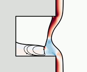
We consider the steady free-surface flow of a viscoelastic liquid film driven by gravity along an inclined plane featuring periodic trenches normal to the main flow direction, see figure 1; for the most part, we will set the inclination angle to  $\alpha = 90^\circ $. In what follows, a superscript ‘*’ will indicate a dimensional quantity. The fluid is incompressible with constant density ${\rho ^\ast }$, surface tension ${\sigma ^\ast }$, relaxation time ${\lambda ^\ast }$ and zero-shear viscosity ${\mu ^\ast } = \mu _s^\ast + \mu _p^\ast $, where $\mu _s^\mathrm{\ast }$ and $\mu _p^\ast $ are the viscosities of the solvent and the polymer, respectively. We assume that the flow is periodic, and the periodicity of the flow spans a single cell of the solid structure (i.e. we do not consider periodic flows with wavelength larger that the size of the unit cell). The unit cell consists of a single rectangular trench of depth ${D^\ast }$ and width ${W^\ast }$ (but we will only consider square trenches, ${D^\ast } = {W^\ast }$), preceded and succeeded by lengths $L_1^\ast $ and $L_2^\ast $ of flat substrate towards the periodic inlet and outlet sides, respectively – see figure 1.

Figure 1. Cross-section of the film flowing over a substrate inclined at an angle  $\alpha $ to the horizontal (shown as $\alpha = 90^\circ $ in the figure) and featuring a trench. The total length of the periodic cell is ${L^\ast }$, while $L_1^\ast $ and $L_2^\ast $ are the entrance and exit lengths before and after the cavity, and ${W^\ast }$ and ${D^\ast }$ represent the width and depth of the cavity, respectively. Here, ${H^\ast }$ is the film height at the inlet, and $H_1^\ast $ and $H_2^\ast $ are the distances of the contact lines along the upstream and bottom cavity walls from the respective corners.
The primary flow parameter is the volumetric flow rate per unit width normal to the depicted cross-section,  ${Q^\ast }$, which determines the thickness H* of the film at the periodic inlet. Under gravity, the liquid film flows downward along the substrate and may partially enter the cavity, where it can form a second interface with the air. The inner interface defines two triple-contact points with the solid wall, one at the upstream sidewall of the trench and the other one at the bottom of the cavity (for cases where the second contact point lies on the downstream sidewall, see Pettas et al. (Reference Pettas, Dimakopoulos and Tsamopoulos2020)). Their location is determined by liquid properties and flow conditions along with the apparent contact angles ${\theta _1}$ and ${\theta _2}$, respectively. At the contact line, there is a sudden change from adherence at the solid surface to no shear along the free surface, which induces a local singularity known to be logarithmically weak and integrable (Michael Reference Michael1958; Richardson Reference Richardson1970). The apparent contact angle is accepted as an overall measure of solid wettability (Kistler & Scriven Reference Kistler and Scriven1994), although different effects may influence this wetting measure (Decré & Baret Reference Decré and Baret2003).
2.1. Governing equations
The governing equations are solved in a non-dimensional form where, as is customary for such flows, lengths and velocities are scaled by the Nusselt flow film thickness,  $H_N^\ast $, and mean velocity, $U_N^\ast $, respectively,
 \begin{equation}H_N^\ast = {Q^{{\ast} 1/3}}{\left( {\frac{{3{\mu^\ast }}}{{{\rho^\ast }{g^\ast }\,\textrm{sin}\,\alpha }}} \right)^{1/3}}\quad \textrm{and}\quad U_N^\ast = {Q^{{\ast} 2/3}}{\left( {\frac{{{\rho^\ast }{g^\ast }\,\textrm{sin}\,\alpha }}{{3{\mu^\ast }}}} \right)^{1/3}}.\end{equation}
The dimensionless continuity and momentum equations are then
 \begin{gather}\boldsymbol{\nabla }\boldsymbol{\cdot }\boldsymbol{u} = 0,\end{gather}
 \begin{gather}Re\,\boldsymbol{u}\boldsymbol{\cdot }\boldsymbol{\nabla }\boldsymbol{u} + \boldsymbol{\nabla }p-\boldsymbol{\nabla }\boldsymbol{\cdot }\boldsymbol{\tau } - \frac{3}{{\textrm{sin}\,a}}\boldsymbol{g} = {\bf 0},\end{gather}
where u = (ux, uy) is the velocity vector (x being the direction parallel to the substrate), p is the pressure,  $\boldsymbol{\tau } = \beta \dot{\boldsymbol{\gamma }} + {\boldsymbol{\tau }_p}$ is the extra stress tensor which can be split into a Newtonian (solvent) part $\beta \dot{\boldsymbol{\gamma }}$ and a polymeric part τp and $\boldsymbol{g} = (\textrm{sin}\,\alpha , - \textrm{cos}\,\alpha )$ is the unit vector in the direction of gravity. The polymeric stress τp evolves according to the dimensionless ePTT constitutive equation
 \begin{equation}Y({\boldsymbol{\tau}_p}){\boldsymbol{\tau }_p} + Wi\,{\mathop{\boldsymbol{\tau}}\limits^\nabla}_p-(1 - \beta )\dot{\boldsymbol{\gamma
}} = {\bf 0},\end{equation}
\begin{equation}Y({\boldsymbol{\tau}_p}){\boldsymbol{\tau }_p} + Wi\,{\mathop{\boldsymbol{\tau}}\limits^\nabla}_p-(1 - \beta )\dot{\boldsymbol{\gamma
}} = {\bf 0},\end{equation}where
 \begin{equation}Y({\boldsymbol{\tau }_p}) = \exp \left( {\frac{\varepsilon }{{1 - \beta }}\,Wi\,\textrm{tr}({\boldsymbol{\tau }_p})} \right),\end{equation}
with tr() being the trace function, while  ${\mathop{\boldsymbol{\tau }}\limits^\nabla}_p = \boldsymbol{u}\boldsymbol{\cdot }\boldsymbol{\nabla }{\boldsymbol{\tau }_p} - {\boldsymbol{\tau }_p}\boldsymbol{\cdot }\boldsymbol{\nabla }\boldsymbol{u} - {(\boldsymbol{\nabla }\boldsymbol{u})^\textrm{T}}\boldsymbol{\cdot }{\boldsymbol{\tau }_p}$ is the upper convected derivative.
The dimensionless numbers in the above equations are the Reynolds number (Re), the Weissenberg number (Wi), the solvent-to-total viscosity ratio β and the ePTT parameter  $\varepsilon $. The definitions of these numbers are presented in table 1. Finite values of the parameter $\varepsilon $ introduce elongational and shear thinning to the fluid model, and set an upper limit to the elongational viscosity.
Table 1. Definitions of dimensionless parameters and numbers,  $l_c^\ast = {({\sigma ^\ast }/{\rho ^\ast }{g^\ast })^{1/2}}$ is the capillary length.

2.2. Boundary conditions
At the inlet and outlet, periodic boundary conditions for velocity and stress are imposed. At the two air–liquid interfaces, a local interfacial stress balance between the capillary force and the stress field is applied, together with the kinematic condition
 \begin{gather}- p\boldsymbol{n} + \boldsymbol{n}\boldsymbol{\cdot }\boldsymbol{\tau } ={-} {p_a}\boldsymbol{n} + C{a^{ - 1}}\frac{{\textrm{d}\boldsymbol{t}}}{{\textrm{d}s}},\end{gather}
 \begin{gather}\boldsymbol{n}\boldsymbol{\cdot }\boldsymbol{u} = 0.\end{gather}
In the above equations, n is the outward unit normal vector to the free surface, pa is the air pressure, which can be set to zero for both interfaces without loss of generality (see Varchanis et al. Reference Varchanis, Dimakopoulos and Tsamopoulos2017 for a discussion of this issue – they found that moderate variations of the pressure inside the air inclusion did not produce any significant changes in the physical phenomena under study), t is the unit tangent vector pointing in the direction of increasing distance ‘s’ along the free surfaces (Ruschak Reference Ruschak1980) and Ca is the capillary number (see table 1).
Along the walls of the substrate, we impose the usual no-penetration and no-slip boundary conditions
 \begin{gather}{\boldsymbol{n}_w}\boldsymbol{\cdot }\boldsymbol{u} = 0,\end{gather}
 \begin{gather}{\boldsymbol{t}_w}\boldsymbol{\cdot }\boldsymbol{u} = 0,\end{gather}
where  ${\boldsymbol{n}_w}$ and ${\boldsymbol{t}_w}$ denote the unit vectors normal and tangential to the wall, respectively. Additionally, at the intersections of the inner interface with the upstream wall and the bottom of the cavity, appropriate boundary conditions for the contact angles need to be imposed. Under steady-state conditions, as in our case, it suffices to define that the contact line is governed by the static angle equations
 \begin{gather}{\boldsymbol{n}_{w1}}\boldsymbol{\cdot }{\boldsymbol{n}_{s1}} = \textrm{cos}\,{\theta _1},\end{gather}
 \begin{gather}{\boldsymbol{n}_{w2}}\boldsymbol{\cdot }{\boldsymbol{n}_{s2}} = \textrm{cos}\,{\theta _2},\end{gather}
where  ${\theta _1}$ and ${\theta _2}$ are the equilibrium contact angles. Furthermore, it will be assumed that ${\theta _1} = {\theta _2} = \theta $, the equilibrium angle characteristic of the particular liquid/solid combination.
For the completeness of the physical model, the film height at the entrance of the unit cell,  ${H^\ast }$, is determined by demanding that the dimensionless flow rate is equal to unity.
2.3. Additional dimensionless numbers
The first four dimensionless parameters in table 1 arise in the dimensionless form of the governing equations and completely define the problem, when the Nusselt thickness (2.1) is chosen as the characteristic length. In several previous parametric studies (e.g. Wierschem et al. Reference Wierschem, Bontozoglou, Heining, Uecker and Aksel2008; Pavlidis et al. Reference Pavlidis, Dimakopoulos and Tsamopoulos2010, Reference Pavlidis, Karapetsas, Dimakopoulos and Tsamopoulos2016; Varchanis et al. Reference Varchanis, Dimakopoulos and Tsamopoulos2017; Sharma et al. Reference Sharma, Ray and Papageorgiou2019) the parameters Re, Ca and Wi (for viscoelastic flows) and the geometric ratios  $L/H_N^\ast $ and $W/H_N^\ast $ were varied individually to determine their effects. While this could be acceptable, it is rather unintuitive and hard to translate into a dimensional experimental setting where it is easiest to vary the flow rate while keeping the same fluid and substrate. The problem is that all of these parameters depend on the flow rate; varying the latter changes all of them. This holds true even for the dimensionless lengths setting the trench geometry. Due to the dependence of the Nusselt flow thickness $H_N^\ast $ (2.1) on the flow rate Q*, the dimensional geometry would vary when the flow rate varies, which is not realistic. Hence, in the present work (as also in previous works Pettas et al. Reference Pettas, Karapetsas, Dimakopoulos and Tsamopoulos2017, Reference Pettas, Karapetsas, Dimakopoulos and Tsamopoulos2019a,Reference Pettas, Karapetsas, Dimakopoulos and Tsamopoulosb; Marousis et al. Reference Marousis, Pettas, Karapetsas, Dimakopoulos and Tsamopoulos2021), we opted to present the results in terms of alternative dimensionless parameters that are easier to vary individually in an experimental setting.
In particular, for our preferred parameters we have retained the Reynolds number but replaced the capillary (Ca) and Weissenberg (Wi) numbers by the Kapitza (Ka) and elasticity (El) numbers, which depend only on the fluid properties and not on the flow rate (table 1). Similarly, distances and dimensions are non-dimensionalized by the capillary length  $l_c^\ast = {({\sigma ^\ast }/{\rho ^\ast }{g^\ast })^{1/2}}$, which, contrary to the Nusselt thickness $H_N^\ast $, does not depend on the flow rate. The resulting non-dimensional substrate dimensions are denoted as L 1, L 2 and W (table 1). Concerning the results, we are particularly interested in the distances $H_1^\ast $ and $H_2^\ast $ of the contact lines along the upstream and bottom cavity walls from the respective corners, as shown in figure 1. The corresponding non-dimensional distances, scaled by the capillary length $l_c^\ast $, are denoted as H 1 and H 2 (table 1). In addition, for the discussion that will follow in the results section, it will be useful to define the Weber number, We, which is a measure of the liquid inertia to the capillary force and takes the flow rate into account (see table 1). Of course, these alternative dimensionless numbers are derivable from the original ones, and $l_c^\ast $ is related to $H_N^\ast $, as follows:
 \begin{gather}We = Ca\,Re,\quad El = \frac{{Wi}}{{R{e^{1/3}}}}{\left( {\frac{3}{{\textrm{sin}\,\alpha }}} \right)^{2/3}}, \end{gather}
 \begin{gather} Ka = \frac{{R{e^{2/3}}}}{{Ca}}{\left( {\frac{{\textrm{sin}\,\alpha }}{3}} \right)^{1/3}},\quad \frac{{l_c^\ast }}{{H_N^\ast }} = \frac{{K{a^{1/2}}}}{{R{e^{1/3}}}}\left( {\frac{{\textrm{sin}\,\alpha }}{3}} \right).\end{gather}
 A main part of the results to be presented concerns holding Ka, El and the geometric ratios L 1, L 2 and W constant and recording the variation of the wetting distances H 1 and H 2 as Re is varied. In an experimental setting, this could be carried out by simply varying the flow rate, using a given fluid and a given substrate. However, it is interesting to note that, due to the dependence of  $H_N^\ast $ on Re expressed by the second of (2.12b), if one wished to hold constant the geometric ratios $L/H_N^\ast $ and $W/H_N^\ast $ instead, then they would have to enlarge the substrate at the same time as the flow rate is increased. This is clearly impractical and highlights the relevance of our alternative non-dimensionalization.
Since the densities of liquids, and even the surface tension, mostly fall within relatively narrow ranges, whereas the viscosity and relaxation time can vary by orders of magnitude, the Kapitza number, Ka, can be viewed roughly as the reciprocal of a dimensionless zero-shear viscosity, and the elasticity number, El, as a dimensionless relaxation time of the fluid. The effects of surface tension can be explored through the capillary length  $l_c^\ast = {({\sigma ^\ast }/{\rho ^\ast }{g^\ast })^{1/2}}$, by increasing or decreasing the dimensionless size of the substrate (L 1, L 2 and W).
2.4. Numerical solution
To solve the above set of equations numerically, we employ the mixed finite element/Galerkin method combined with an elliptic grid generator (Dimakopoulos & Tsamopoulos Reference Dimakopoulos and Tsamopoulos2003) to account for the highly deformable flow domain. Due to the hyperbolic character of the constitutive equation and to preserve the numerical stability of the scheme, we employ the SUPG/DEVSS-G (Guénette & Fortin Reference Guénette and Fortin1995) method that has been successfully used in the past for the solution of viscoelastic flows (Pettas et al. Reference Pettas, Karapetsas, Dimakopoulos and Tsamopoulos2015; Varchanis et al. Reference Varchanis, Dimakopoulos, Wagner and Tsamopoulos2018, Reference Varchanis, Syrakos, Dimakopoulos and Tsamopoulos2019, Reference Varchanis, Syrakos, Dimakopoulos and Tsamopoulos2020, Reference Varchanis, Pettas, Dimakopoulos and Tsamopoulos2021). Finally, to trace the steady-state solution in parameter space, pseudo-arc-length continuation is employed. According to this method the continuation step in one of the parameters is not constant, but is implicitly calculated by requiring the next state to have a constant arc-length distance from the previous one, see Pettas et al. (Reference Pettas, Karapetsas, Dimakopoulos and Tsamopoulos2017) and Varchanis et al. (Reference Varchanis, Dimakopoulos and Tsamopoulos2017) for more information. The code employed is similar with the one used for our previous study that concerned flow over a slit rather than trench geometries (Pettas et al. Reference Pettas, Dimakopoulos and Tsamopoulos2020). The presently employed mesh resolutions were selected based on our previous experience. We refer the reader to the previous study (Pettas et al. Reference Pettas, Dimakopoulos and Tsamopoulos2020) for mesh convergence results and validation of the code by comparison with previously published results that were obtained using an entirely different solver (OpenFOAM, employing the volume-of-fluid method and transient finite volume simulations). Despite the presence of sharp corners, where stress magnitudes are theoretically infinite but integrable, the effect of these corners is highly localized and does not significantly impact grid convergence. Some indicative grid convergence results are presented in Appendix A.
3. Results and discussion
3.1. General pattern
We begin with a presentation of the general pattern of Newtonian flow and its dependence on the flow rate as reflected by the Reynolds number in figure 2 (note the increase of the film thickness at the inlet of the domain with  $Re$ in the insets). This will help the reader become familiar with the flow and serve as a basis for comparison for the non-Newtonian results to follow. We will not discuss this figure in detail since extensive Newtonian results can be found in Varchanis et al. (Reference Varchanis, Dimakopoulos and Tsamopoulos2017). Figure 2(a,b) shows the dependence of the wetting lengths ${H_1}$ and ${H_2}$ on the flow rate (reflected in the $Re$), along with a few representative film shapes and streamline patterns at specific Reynolds numbers. The problem parameters are: vertical substrate ( $\alpha = 90^\circ $), contact angle of $\theta = 60^\circ $, Ka = 2 and square trenches with W = D = L 1 = L 2 = 7. At least two independent equilibrium states coexist for most of the range of $Re$ for which simulations were performed; they will be referred to as the upper family (drawn in dashed line in figure 2) and the lower family (drawn in continuous line). In figure 2 and similar figures, solution families are represented by lines of varying styles for easy differentiation, while line colours indicate different constant parameter values as Re is varied. These lines are created by interpolating between successive solution points obtained through the arc-length continuation procedure. However, the interpolation error is negligible due to the close spacing of the data points – see Appendix B for an example.

Figure 2. Map of the steady-state solutions for a Newtonian liquid in terms of the wetting lengths at the (a) upstream wall,  ${H_1}$, and (b) downstream wall, ${H_2}$, for $Ka = 2$, $\theta = 60^\circ $, ${L_1} = {L_2} = W = D = 7$. The lower and upper solution branches are drawn in different line styles, (———) and (– - – - –), respectively. Insets (i)–(vi) depict the flow patterns at the points marked by symbols in the main diagrams.
Concerning the upper family, at very small flow rates, the liquid enters deeply into the topographical feature, leading to almost full coating; only a tiny air inclusion remains close to the upstream wall, as can be seen in the inset (i) of figure 2. In fact, increasing the flow rate causes the air inclusion to contract even more, with the inclusion size thereafter remaining approximately constant in the range  $0.5 \le Re \le 5$ – see inset (ii) of figure 2. For Re < 5, apart from the small air inclusion, the flow configuration resembles liquid films over fully coated substrates, with the outer interface exhibiting a large depression into the trench. This penetration and near-full coating is caused by surface tension, which gives rise to an inward pressure gradient due to the interface curvature at the entrance corner by the adhesive force at the contact lines. This flow configuration is, therefore, shaped mostly by capillarity and gravity, and we will refer to the set of such flows as the ‘capillary-gravity’ region (Re < 5 in this case), following Varchanis et al. (Reference Varchanis, Dimakopoulos and Tsamopoulos2017).
However, an increase of the flow rate above this range (Re > 5) brings about a dramatic change in the flow configuration, with the main flow stream becoming detached from the bottom of the cavity, as seen in inset (iii) of figure 2, as the momentum of the liquid is now too large for capillarity to deflect it. Nevertheless, the space between the main liquid stream and the bottom of the trench becomes occupied by a large zone of recirculating liquid. Hence, the drastic change of the flow configuration is not so much reflected in the variation of the wetting lengths H 1 and H 2 in figure 2. The recirculation zone at the bottom of the cavity moves so as to stretch the air inclusion in the y-direction causing it to expand along the upstream wall – see inset (iii) of figure 2. The vortex, whose strength increases with increasing Re, contains fluid that is not replenished, while the rest of the flow bypasses the bottom of the cavity, due to the effect of inertia and it being pulled across by gravity. Because the factors that mostly determine this flow configuration are inertia and gravity, this flow regime will be called the ‘inertia-gravity’ regime (Varchanis et al. Reference Varchanis, Dimakopoulos and Tsamopoulos2017).
Very different flow patterns are observed in the lower solution family, characterized by much larger air inclusions. At low values of  $Re$ the liquid wets only slightly the upstream wall of the cavity while the film falls almost vertically under the action of gravity, forming a thin, almost straight liquid bridge across the gap – see inset (iv) in figure 2. This film does not penetrate deep along the upstream wall but flows towards the outlet. The downstream wall is, however, fully covered by a layer of liquid, but most of it recirculates in the form of a sequence of vortices and is separated from the main flow. The effects of inertia are negligible, and this flow configuration is determined by a balance of gravity, capillarity and viscosity. As the Reynolds number is increased beyond $Re = 1$, the contact line of the upstream wall begins to move deeper into the cavity, as the pressure gradient due to the interface curvature at the trench entrance corner causes the liquid to travel along to the upstream sidewall up to a point, with H 1 reaching a maximum value of ${H_{1,max}} = 2.48$ at $Re \approx 3.25$, see figure 2. The liquid bridge also penetrates deeper into the cavity, and the wetting length H 2 increases as well, reducing the volume of trapped air – see inset (v) in figure 2. However, a further increase of the flow rate beyond this value causes a reversal of the previous trend, with H 1 decreasing again. Furthermore, at $Re \approx 3.79$ and 3.61 two successive turning points arise, see figure 2, defining a hysteresis loop that resembles the hydrodynamic hysteresis observed by Kistler & Scriven (Reference Kistler and Scriven1994) in the so-called teapot effect. For a narrow range of $Re$ ( $3.61 \le Re \le 3.79$), three different steady states coexist within this lower solution family, with distinctly different flow patterns. At even higher flow rates (inset (vi) in figure 2), the upstream wall is almost completely dry, as the fluid inertia is too large for the pressure gradient to handle, merely causing the film to fall at an inward angle but not being able to force it to adhere to the upstream sidewall. The momentum of the liquid bridge across the gap intensifies and takes the form of a jet, which impinges on the vortex at the downstream bottom corner of the cavity causing it to swell, increasing the wetting length H 2. Due to the high momentum of the falling film, a cusp forms at the point of intersection of the film with the rotating vortex, whose sharpness creates numerical difficulties that did not allow us to advance the parametric continuation on the lower family beyond $Re = 7.12$.
We can apply the same flow characterization to the lower solution family as well. At low flow rate values  $(Re < 1)$, capillarity prevails since inertia is relatively weak, with the Weber number having very small values. This region is called the ‘capillary-gravity’ region in Varchanis et al. (Reference Varchanis, Dimakopoulos and Tsamopoulos2017), since the position of the contact lines is an outcome of a balance between surface tension and gravity. On the other hand, at high values of flow rate ( $Re > 4$) inertia, which tends to dewet the upstream wall, dominates over capillarity and the wetting distance over that wall is minimized. As previously mentioned, the flow pattern changes abruptly as we pass through the hysteresis loop. Interestingly, Varchanis et al. (Reference Varchanis, Dimakopoulos and Tsamopoulos2017) found that the second turning point of the hysteresis loop arises under constant values of the Weber number, indicating that there is a delicate balance between inertia and surface tension that signifies the onset of the ‘inertia-gravity’ region. At intermediate values of $Re$ ( $1 < Re < 4$), neither inertia nor surface tension dominates the flow, however, and the interplay between the capillary, viscous and inertia forces pulls the film inside the cavity. In the rest of the paper, we will examine how the introduction of non-Newtonian effects impacts the flow configuration and the wetting lengths in particular.
3.2. Effect of fluid elasticity
In figure 3(a,b), we present the variation of the wetting lengths  ${H_1}$ and ${H_2}$, respectively, as a function of $Re$ for various values of $El < 1$, while the other rheological parameters are held at $\varepsilon = 0.1$ and $\beta = 0.1$. As mentioned, the rheological parameter $\varepsilon $ of the ePTT model imparts both elongational and shear thinning to the fluid, and it establishes an upper limit for the elongational viscosity. However, for low values of $El$ such as these ( $El < 1$) shear thinning is notably mild (Pavlidis et al. Reference Pavlidis, Karapetsas, Dimakopoulos and Tsamopoulos2016). This specific regime of viscoelastic flow with small shear thinning is the focus of the present section. Overall, in figure 3(a,b) we observe that the fluid elasticity has the opposite impact on the two solution families. Starting from the upper solution family, it is interesting to note that the wetting length ${H_1}$ is almost unaffected by elasticity up to $Re \approx 5$, i.e. in the capillary-gravity regime, while ${H_2}$ is almost unaffected for all values of Re examined. Beyond Re = 5, in the regime where the liquid stream is detached from the upstream sidewall and a large recirculation zone has developed, increasing the elasticity number causes the wetting length H 1 to decrease less with Re compared with the Newtonian case. Insets (i, ii) in figure 3 illustrate the corresponding streamline patterns calculated at $El = 0.5$ and $Re = 7$ in the lower and upper solution families, respectively. Under the same flow rate, the presence of fluid elasticity attenuates the intensity of the vortex, allowing the air inclusion to maintain a smaller and more circular shape. Thus, ${H_1}$ increases with increasing $El$, but only up to a point (e.g. H 1 varies very little between El = 0.5 and 0.75). That this effect is noticeable only for $Re \ge 5$ is because it is only at these Reynolds numbers that a vortex is formed (see figure 2).

Figure 3. Solution families for the wetting length (a)  ${H_1}$ and (b) ${H_2}$ for various values of the elasticity number for $Ka = 2$, $\varepsilon = 0.1$, $\beta = 0.1$, ${L_1} = {L_2} = W = D = 7$. The colours of the lines correspond to different values of $El$, while the lower and upper solution branches are drawn in different line styles, (———) and (– - – - –), respectively. Insets (i, ii) depict the flow of viscoelastic films with $El = 0.5$ and $Re = 7$ located at the lower and upper solution families, respectively.
At the lower solution family, elasticity has the opposite effect with respect to the volume of the air inclusion, as  ${H_1}$ and ${H_2}$ decrease monotonically as $El$ increases, see figure 3(i). It is interesting to note in figure 3(a) that the introduction of elasticity to the fluid eliminates the hysteresis loop and smooths the transition to the inertia regime of the flow. The smoothening is more prominent at higher values of the elasticity number, with ${H_{1,max}}$ decreasing considerably, falling to ${H_{1,max}} \approx 0.67$ for $El = 0.75$. The other wetting length, H 2, follows the same trend as H 1. In fact, it was observed that this is almost always the case, and hence in the rest of the paper we will focus mainly on H 1.
The spatial variation of the xx-component of the polymeric stress tensor,  ${\tau _{p,xx}}$, is depicted in figure 4(i,ii), along with some streamlines, for $El = 0.75$ and $Re = 2.5$ for steady states that belong to the upper and lower solution families, respectively. In both cases, the axial normal stress is maximized along the entrance and exit walls, outside the trench, but things change in the rest of the domain. As indicated in figure 3, at this value of Re elasticity has a negligible impact on the upper family but a significant impact on the lower one; figure 4 helps to explain why. For the upper family, as noted, at this low value of Re there is no recirculating vortex and the fluid enters deep into the trench and it is decelerated by its walls (figure 4i); consequently, it becomes thicker than in the domain entrance and with lower velocity, which results in lower viscoelastic stresses. Hence, polymeric stresses have negligible impact on the shape and position of the inner interface, including the two contact lines. In contrast, the flow configuration corresponding to the lower family, as shown in figure 4(ii), displays a film that moves straight down, being accelerated by gravity and experiencing lower viscous resistance, which makes it narrower than in the entrance. This results in considerably higher velocities and associated stretching of the polymeric chains and leads to substantially elevated normal elastic stresses. One notices particularly high values of viscoelastic stress at the entrance corner of the cavity, which do not allow the contact line to travel deeply along the upstream wall, i.e. they keep H 1 small. Therefore, as $El$ increases, ${H_1}$ will decrease. On the other hand, as the liquid approaches the downstream wall, the flow cross-section increases, the liquid is decelerated as it spreads to coat the downstream trench wall. The resulting recirculation is rather weak, and the normal polymeric stress field is similarly weak. Hence, changes in $El$ do not affect ${H_2}$. It should be noted that, because in both cases El and Re have the same values, the Weissenberg number will have the same value as well (see (2.12a)) and, hence it cannot explain the difference between the two flows depicted in figure 4.

Figure 4. Spatial variation of the normal polymeric stress field,  ${\tau _{p,xx}}$ for steady states that belong to (i) the upper and (ii) the lower solution families, respectively. The flow parameters are $Re = 2.5$, $Ka = 2$, $El = 0.75$, $\varepsilon = 0.1$ and $\beta = 0.1$.
3.3. Combined effect of elasticity and shear thinning
The ePTT model predicts that the steady shear viscosity is constant at low shear rates but decreases at higher shear rates (shear thinning); this mirrors the typical behaviour of most polymeric fluids. Shear thinning can become particularly steep for the ePTT model. The onset of shear thinning occurs at lower shear rates as λ*, or El in our non-dimensional setting, is increased. An increase of the model parameter ε leads to the same outcome. In fact, the onset of shear thinning in simple shear flow is governed by the product  $\varepsilon {\lambda ^{{\ast} 2}}$, rather than the individual values of $\varepsilon $ or λ* (refer to Appendix 1 of Syrakos, Dimakopoulos & Tsamopoulos Reference Syrakos, Dimakopoulos and Tsamopoulos2018). At the relatively low values of $El$ that we examined in the previous paragraph, shear thinning was small, and elasticity had the effect of preserving the high viscoelastic stresses generated at high deformation zones, enabling them to propagate over greater distances and amplifying their significance in shaping the flow compared with the Newtonian case. However, when $El$ surpasses a certain threshold, shear thinning becomes dominant, leading to a reduction in the magnitude of the viscoelastic stresses. Consequently, the prominence of viscoelastic stresses diminishes in comparison with other flow drivers, such as capillarity, inertia and gravity, causing the effects observed in the previous paragraph to be reversed.
Figure 5 illustrates the variation of the wetting length  ${H_1}$ as a function of the Reynolds number for a range of elasticity numbers ( $El$ spanning from 1 to 4) that are higher than those examined in the preceding section. When juxtaposed with figure 3(a), it becomes evident that increasing $El$ from 1 to 4 counteracts the effects that were caused by increasing El from 0 to 0.75. This observation holds true for both solution families and aligns with the explanation provided earlier. Considering first the lower solution family, increasing $El$ from 1 to 4 causes the maximum value of ${H_1}$ to increase from ${H_{1,max}} = 0.56$ to ${H_{1,max}} = 1.02$. This effect is primarily associated with the shear thinning that arises for higher values of $El$, reversing the impact of elasticity on the wetting length by decreasing the liquid viscosity. Inset (i) in figure 5 depicts the spatial variation of the shear polymeric stress field, ${\tau _{p,yx}}$, for a steady state that belongs to the lower solution family at $Re = 2.8$. It obtains large values at the flat part of the substrate before (and after) the trench, causing viscosity to decrease locally, lowering the stresses that inhibited the upstream contact line from advancing deeper into the trench along the upstream wall at lower $El$ values. Hence, ${H_1}$ increases. Apart from the flat part of the substrate, the liquid bridge across the cavity is an almost shear-free region.

Figure 5. Variation of the wetting length  ${H_1}$ as a function of $Re$ for various values of $El$. The colours of the lines correspond to different values of $El$, while the lower and upper solution branches are drawn in different line styles, (———) and (– - – - –), respectively. Inset (i) shows the spatial variation of the ${\tau _{p,yx}}$ field for $El = 4$ and $Re = 2.8$, at the lower solution family. Inset (ii) shows the spatial variation of the ${\tau _{p,yx}}$ field for $El = 4$ and $Re = 10$, at the upper solution family. The remaining fluid parameters in both cases are $Ka = 2$, $\varepsilon = 0.1$, $\beta = 0.1$.
The flows that comprise the upper solution family exhibit a larger contact area with the cavity walls, which can cause the shear-thinning effects to be felt deeper inside the cavity. Figure 5 shows that an increase of El from 1 to 4 for  $Re > 6$ tends to stretch the enclosed air bubble along the upstream wall, reducing the wetting length ${H_1}$ to values close to those of the Newtonian flow. Inset (ii) in figure 5 shows the spatial variation of ${\tau _{p,yx}}$ for $Re = 10$. In this case, the liquid stream travelling across the gap is not bounded by the inner interface but is in contact with other liquid that forms a vortex. Shear stresses develop in the shear layer between the main flow and the vortex, giving rise to shear thinning that causes the viscosity to drop and the stresses to be lower than in lower $El$ cases. This in turn intensifies the vortex inside the cavity, which stretches the air inclusion in the y direction.
Interestingly, for  $El = 3$ and 4, at moderate values of $Re$, the upper family exhibits multiple steady states, connected via turning points and forming hysteresis loops. These loops occur at $5.94 \le Re \le 6.34$ for El = 3 and at $4.51 \le Re \le 5.34$ for El = 4 (see figures 5 and 6), close to the transition between the capillary-gravity and inertia-gravity regimes. To investigate this further, figure 6 shows a close-up of the hysteresis loop for $El = 4$ together with insets (i–iii) presenting contours of ${\tau _{p,yx}}$ for the various steady states at $Re = 5$. At low values of $Re$, the air inclusion has an almost circular cross-section, and it is located close to the upstream concave corner, similarly to the Newtonian case. This arrangement lasts until approximately $Re = 5$; inset (i) of figure 6 shows this flow configuration together with the corresponding ${\tau _{p,yx}}$ field. For $Re < 5$ the film coats almost entirely the trench and the elevated values of shear stress that occur over most of the length of the solid walls, both inside and outside of the trench, cause extensive shear thinning that leads to an increase of the effective (local) Reynolds number. As a result, the effect of inertia becomes important even though the nominal Reynolds number is still moderate. At $Re = 5.34$ a turning point arises, and any further increase in the flow rate causes an abrupt change in the flow configuration, where the fluid detaches from a large portion of the walls of the trench, and the air inclusion grows considerably, as in inset (iii) of figure 6. This detachment, and the concomitant formation of a low-shear liquid bridge, result in overall decreased levels of shear stress (and higher values of viscosity). Between these states, the hysteresis loop contains intermediate steady states such as that of inset (ii) of figure 6. Following basic ideas of bifurcation theory and making the reasonable assumption that the flow is stable for small $Re$, we may conclude that shapes (i) and (iii) are stable (observable) and shape (ii) is unstable.

Figure 6. Enlarged view of the upper solution family close to the hysteresis loop of for  $El = 4$, $Ka = 2$, $\varepsilon = 0.1$, $\beta = 0.1$. The colour contours show the spatial variation of the ${\tau _{p,yx}}$ field. Insets (i)–(iii) indicate flow arrangements for the same $Re = 5$ at the three branches of the hysteresis loop.
With further increase of  $Re$, the wetting length ${H_1}$ increases again as the depression of the outer gas–liquid interface moves towards the downstream wall. Then, a second hysteresis loop is observed at slightly higher values of $Re$,
$Re$,  $6.31 \le Re \le 6.71$ – see figure 6. As showed by Varchanis et al. (Reference Varchanis, Dimakopoulos and Tsamopoulos2017), this latter hysteresis can be attributed to the ballistic-like effect, where the fluid is being ejected from the upstream substrate wall with inertia and gravity pulling it downwards, while the pressure gradient caused by the upstream contact line pulls it inwards.
The effect of further increases of  $El$ is illustrated in figure 7. One can observe dramatic changes in the flow patterns at moderate values of $Re$. For $El = 4.97$, the maximum value of H 1 of the lower solution family and the minimum value of H 1 of the upper family are nearly equal: ${H_1} = 2.16$ and 2.23, respectively. At $El = 5.02$ these values become exactly equal (not shown in figure 7), and the two solution families merge: the second turning point of the upper hysteresis loop coincides with the first turning point of the lower solution family at a perfect transcritical bifurcation (Seydel Reference Seydel2010). For values of El larger than 5.02, the wetting curves are split, creating two individual curves. In other words, El is the parameter that breaks the symmetry of this transcritical bifurcation, when it assumes values larger or smaller than 5.02. The shapes of the two rearranged families for $El > 5.02$ are represented in figure 7 by $El = 8$. At lower flow rates ( $0 \le Re \le 3.44$ for $El = 8$, see figure 7), the steady states of the capillary-gravity region form a closed isola, while at higher flow rates ( $Re \ge 3.08$ for $El = 8$, see figure 7) the inertia-gravity region has its own detached curve. There is no continuous transition between the two regimes, as the curves are not connected. We observe that the wetting length ${H_1}$ increases very rapidly with increasing $Re$ in the intermediate Re range, on the parts of both curves that face each other. For example, on the capillary-gravity (left) isola, for $El = 8$, ${H_1}$ increases from 0.54 to 4.64 as Re increases from $Re = 1$ to $Re = 3.5$. Insets (i, ii) in figure 7 depict the spatial variation of ${\tau _{p,yx}}$ for $Re = 2$ and 3.5, respectively. The wetting length increase seems to be associated with the strong shear stress increase that is observed in the proximity of the upstream wall, which causes shear thinning. The detachment of the two curves means that the flow pattern does not change smoothly as the flow rate is increased, but there must be an abrupt change as we jump from one curve to the other.

Figure 7. Solution families for the wetting length  ${H_1}$ as a function of $Re$ for $El = 4.97$ and $El = 8$. Insets (i, ii) depict the spatial variation of the ${\tau _{p,yx}}$ field for $Ka = 2$, $El = 8$, $\varepsilon = 0.1$, $\beta = 0.1$. The colours of the lines correspond to different values of $El$, while the different styles of the line, (———), (– - – - –), represent the lower, upper, solution branches, respectively. The two insets correspond to the points indicated in the graph and depict the film shapes and the ${\tau _{p,yx}}$ field.
Shear thinning is intensified not only by increasing El, but also by increasing ε. In fact, one could argue that ε is a clearer indicator of the shear-thinning intensity as the relaxation time (or El in dimensionless terms) appears also in the time derivative term of the PTT constitutive equation and therefore has a more complex role. It is, therefore, ε that we now turn our attention to. In figure 8(a) we present the wetting curves for different values of  $\varepsilon $. In general, $\varepsilon $ controls both shear and elongational thinning. In the special case $\varepsilon = 0$ the ePTT model is reduced to the Oldroyd-B model, which does not exhibit any shear thinning. Indeed, in figure 8 we observe that variation of the value of ε has a qualitatively similar effect to a variation in $El$. For $\varepsilon = 0.05$ the wetting length on the lower solution family is kept small throughout the range of $Re$, indicating that the intense elastic stresses that arise at small values of $\varepsilon $ prevent the upstream contact line from advancing inwards along the upstream wall. It should be mentioned that, in the limit of $\varepsilon = 0$ (Oldroyd-B fluid – results not shown), we cannot find any solution with ${H_1} \ne 0$, meaning that high elasticity prevents the fluid from wetting the upstream wall and pins the corresponding contact line at the convex corner. At such low values of $\varepsilon ( = 0.05)$, the air inclusion at the upper solution family has an almost circular cross-section up to $Re \approx 7$. When $\varepsilon $ is increased, the corresponding wetting length at the lower and upper solution families is affected considerably and at a critical value of ε the two families intersect at a transcritical bifurcation; further increase of ε leads to a separation of the capillary-gravity and inertia-gravity regions. All these phenomena mirror those that occur when $El$ is increased instead, whereas here $\varepsilon $ plays the role of the parameter breaking the symmetry.

Figure 8. (a) Solution families for the wetting length  ${H_1}$ as a function of $Re$ for various values of the rheological parameter $\varepsilon $. The remaining parameters are $Ka = 2$, $El = 4$, $\beta = 0.1$. The colours of the lines correspond to different values of $\varepsilon $, while the different line styles, (———), (– - – - –), (- - - - - - -) and (—⋅⋅⋅—), represent the lower, upper, left and right solution branches, respectively. (b) Critical conditions for the transcritical bifurcation in the $({Wi,\varepsilon } )$-plane, for Re = 3.5.
In fact, the same phenomena (appearance of the transcritical bifurcation, separation of the capillary-gravity and inertia-gravity regions) are observed also in Newtonian fluids when the Kapitza number is increased, as shown by Varchanis et al. (Reference Varchanis, Dimakopoulos and Tsamopoulos2017). Higher Kapitza numbers mean smaller viscosity, so this lends support to the attribution, in the present case, of these phenomena to shear thinning rather than to elasticity.
In figure 8(b) we present the critical conditions, in the  $(Wi,\varepsilon )$ plane, for the occurrence of the transcritical bifurcation, for a value of Re = 3.5. The plane is split into subcritical and supercritical conditions. Note that the Weissenberg number and elasticity number are proportional to each other via the expression given by (2.12a), and $El$ is indicated in the right y-axis. As anticipated, the critical value of $Wi$ rapidly increases as the ePTT model approaches the Oldroyd-B model ( $\varepsilon $ decreases); for example, it equals 3.07 and 7.49 for $\varepsilon = 0.1$ and 0.05, respectively. The elimination of shear thinning from the viscoelastic model, as well as the higher elastic response that arises as $\varepsilon \to 0$, cause the critical value of $Wi$ to increase.
3.4. Effect of zero-shear viscosity
Figure 9(a) illustrates the dependence of  ${H_1}$ on the Reynolds number for different values of the Kapitza number. Given that the gravitational acceleration is constant, and the density of most fluids lies within a narrow range, $Ka$ reflects the relative importance of surface tension compared with the zero-shear viscosity; therefore, smaller values of $Ka$ correspond to more viscous liquids (compared with their surface tension). According to the results of the previous paragraph, where the effects of increasing the elasticity number and the rheological parameter ε were attributed (beyond a certain limit) to shear thinning, one would expect that increasing Ka has a similar effect. Indeed, this is verified by figure 9(a), which shows that increasing Ka eventually gives rise to a transcritical bifurcation, beyond which the capillary-gravity and inertia-gravity regions are completely separated. A difference from the trends observed when increasing the $El$ or $\varepsilon $ numbers is that an increase in Ka seems to push the inertia-gravity region to higher Reynolds numbers (figure 9a). For example, the lower turning point of the curves of that region (or, in the case prior to the occurrence of the transcritical bifurcation, the second turning point of the hysteresis loop at the lower solution family) is calculated to occur at $Re = 3.50$, 3.94 and 4.9 for $Ka = 2.5$, 3 and 4, respectively. However, plotting ${H_1}$ as a function of the Weber number, $We$, instead of Re, as in figure 9(b), these points can be seen to occur at the same value of $We = 2.24$, where the onset of the inertia-gravity region occurs through a delicate balance between inertia and capillary forces. This has been observed also by Pettas et al. (Reference Pettas, Karapetsas, Dimakopoulos and Tsamopoulos2017) and Varchanis et al. (Reference Varchanis, Dimakopoulos and Tsamopoulos2017), and a detailed explanation based on scaling arguments is presented in Pettas et al. (Reference Pettas, Dimakopoulos and Tsamopoulos2020).

Figure 9. Solution families for the wetting length  ${H_1}$ as a function of (a) $Re$ and (b) $We$ for various values of $Ka$. The remaining fluid parameters are $El = 3$, $\varepsilon = 0.1$, $\beta = 0.1$. The colours of the lines correspond to different values of $Ka$, while the different styles of the line, (———), (– - – - –), (- - - - - - -) and (—⋅⋅⋅—), represent the lower, upper, left, and right solution branches, respectively.
3.5. Effect of the geometry
Having examined the effect of the fluid properties on the flow configuration, we now turn to the substrate geometry. First, we will examine the effect of the distance between the trenches. Figure 10 illustrates the effect of the lengths L 1 and L 2 of the inflow and outflow regions of the periodic unit cell on the wetting length  ${H_1}$ while the size of the cavities is kept constant. Insets (i) and (ii) in figure 10 depict the film shapes and the contour plots of the polymeric shear stress for ${L_1} = {L_2} = 3$ and ${L_1} = {L_2} = 7$, respectively. Note that the presented steady-state profiles were calculated at the upper solution family for $Re = 6$, see symbols in figure 10. Interestingly, the upper solution family is affected the most by the variation of the inflow and outflow lengths, since the hysteresis loop that arises in the range of $5.94 \le Re \le 6.34$ for ${L_1} = {L_2} = 7$ is eliminated when the periodic trenches are packed closer to each other (see figure 10 for ${L_1} = {L_2} = 5$ and 3). As can be seen in insets (i, ii) in figure 10, at large values of $Re$ the film forms an inertia ridge as it exits the cavity with momentum in the cross-wise direction (Kalliadasis et al. Reference Kalliadasis, Bielarz and Homsy2000). This ridge can persist for 6 or more unit lengths downstream of the exit corner, beyond which a fully developed flow is established along the flat substrate. Comparing insets (i) and (ii) of figure 10, one notices that, when the distance between the trenches is small (inset (i) in figure 10), then the liquid reaching the entrance of a trench is still accelerating, as deduced from the tapering form of its free surface, whereas at larger trench distances (inset (ii) of figure 10), a higher, terminal (fully developed) velocity is reached – this means that inertial effects are more pronounced in large-spacing configurations. Also, the acceleration of the fluid in the x-direction, indicated by the tapering of the film, leads to fluid extension, contributing to the development of normal stresses. At large trench distances, when the fluid reaches the next trench, it has achieved a fully developed flow profile, allowing this component of the normal stresses to relax. However, in more closely packed trenches, the fluid entering a trench is still accelerating, hence this component of the stresses is present, influencing the dynamics. Finally, another effect of increasing the inter-trench distance is that shear thinning is intensified because the fluid undergoes shearing over longer distances (compare the shear stress distributions of insets (i) and (ii) in figure 10). Indeed, the changes observed in the upper family in figure 10 as the lengths ${L_1}$ and ${L_2}$ are increased are reminiscent of those described in the previous sections in relation to shear thinning. Interestingly, figure 10 shows that the variation of the distance between the trenches has no effect on the lower solution family.

Figure 10. Solution families for the wetting length  ${H_1}$ as a function of $Re$ for various lengths of the inflow and outflow regions. Insets (i) and (ii) show the spatial variation of the ${\tau _{p,yx}}$ field for ${L_1} = {L_2} = 3$ and ${L_1} = {L_2} = 7$, respectively, for $Re = 6$ at the upper solution family. The remaining fluid parameters are $El = 3$, $\varepsilon = 0.1$ and $\beta = 0.1$. The colours of the lines correspond to different values of L 1 = L 2, while the different styles of the lines, (———), (– - – - –), to the lower and the upper solution branches, respectively.
In figure 11, the wetting length at the upstream wall is plotted as a function of Re for different sizes of the square trenches. Examining the lower solution family, we see that increasing the trench size has only a marginal impact on  ${H_1}$. This can be attributed to the very small dependence on the trench size of the normal polymeric stress field close to the upstream wall (see insets (i) and (ii) in figure 11), since for this flow configuration it is the stresses near the upstream corner that mostly determine the penetration of the liquid along the upstream wall. Midway across the trench the film is falling freely. Thus, its neck becomes thinner with increasing W due to the acceleration by gravity, and the velocity locally increases. Therefore, in inset (ii) figure 11 we see high values of normal stress inside the liquid bridge, until it reaches its minimum thickness near the downstream wall. When it merges with the liquid residing on the downstream wall it undergoes a sudden compression, hence the negative axial stresses. Comparing insets (i) and (ii) figure 11, one sees that the downstream wetting distance ${H_2}$ also does not change appreciably on increasing the trench size $D = W$ from 5 to 8; the downstream contact line is located approximately 2 unit lengths away from the downstream concave corner in both cases. Therefore, an increase of the size of the cavity results in an enlargement of the volume of the air enclosed inside the topographical feature.

Figure 11. Solution families for the wetting length  ${H_1}$ as a function of $Re$ for different sizes of the square trenches. Insets (i, ii) show the spatial variation of the ${\tau _{p,xx}}$ field for $W = D = 5$ and $W = D = 8$, respectively, for $Re = 2.5$, at the lower solution family. The remaining fluid parameters are $Ka = 2$, $El = 3$, $\varepsilon = 0.1$ and $\beta = 0.1$. The lengths ${L_1}$ and ${L_2}$ remain equal to 7. The colours of the lines correspond to different values of $W = D$ while the different styles of the line, (———) and (- - - - - - -), indicate the lower and the upper solution families, respectively.
On the other hand, at the upper solution family, the flow configuration is such that the liquid wets a much larger portion of the trench's walls, and therefore it is anticipated that shear-thinning effects will become more prominent as the size of the trench increases, as increasing the trench's size increases also the high-shear contact area between the liquid and the cavity walls. Indeed, figure 11 shows that, while at small trench sizes a hysteresis loop is absent from the upper family, at larger sizes such a loop appears, and its intensity has a positive correlation with the trench size. As previously argued, the appearance of this hysteresis loop is associated with shear-thinning effects.
3.6. Effect of the contact and inclination angles
Figure 12(a) presents the solution families of the wetting distance  ${H_1}$ for different values of substrate wettability as a function of Re. The wetting distances depend strongly on the apparent contact angle since, the more hydrophilic the substrate, the larger the inward force applied on the contact point, $F_{CL}^\ast = {\sigma ^\ast }\,\textrm{cos}\,\theta $. The contact angles do not affect qualitatively the bounds of the regimes defined and analysed in the previous sections, although in comparison with our base case of $\theta = 60^\circ $, for $\theta = 45^\circ $ the entire lower solution family has moved upwards, as the film enters deeper along the trench's upstream wall. Note that this increase in ${H_1}$ is observed even under creeping flow conditions, which is something that was not observed when varying any of the other parameters. At the same time, the transition to the ‘inertia-gravity’ regime is shifted to larger values of $Re$, which is reasonable as greater inertia is needed to overcome the greater surface tension force. At even smaller values of $\theta $ (for $\theta = 30^\circ $ in figure 12a), we observe that we have surpassed the familiar transcritical bifurcation and the splitting of the capillary-gravity and inertia-gravity regions. These abrupt changes seem to occur at intermediate Reynolds numbers when the capillary force is strong compared with the viscous stresses.

Figure 12. Solution families for the wetting length  ${H_1}$ as a function of $Re$ for various values of (a) substrate wettability and (b) inclination angle. The remaining fluid parameters are $Ka = 2$, $El = 3$, $\varepsilon = 0.1$, $\beta = 0.1$, while the trench has lengths $L = W = 7$. The colours of the lines correspond to different values of $\theta $ and $\alpha $, while the different styles of the line, (———), (– - – - –), (- - - - - - -) and (—⋅⋅⋅—), represent the lower, upper, left, and right solution branches, respectively.
In many cases of coating processes, the inclination angle is not fixed at  $\alpha = 90^\circ $, so before completing our study we will briefly consider the effect that the inclination angle has. In figure 12(b), the impact of the orientation of the substrate on the evolution of the solution families is presented as a function of the flow rate. For $\alpha = 85^\circ $ we observe in the lower family an increase in the wetting distance H 1, while the capillary gravity-region forms again an isola in the ${H_1}$– $Re$ diagram, and there is no continuous transition to the inertia-gravity region. These phenomena are intensified at $\alpha = 70^\circ $; as the $y$-component of the gravity vector increases, so does the wetting distance of the flow, while the separation between the two flow regions becomes greater (figure 13). This can be explained by noting that, by inclining the substrate, a component of gravity pulls the liquid inside the trench, aiding the capillary forces in their competition with the viscous forces, similarly to shear thinning and wettability. In figure 13, inclination is also seen to increase H 2 substantially, causing an overall decrease in the volume of the enclosed air. On the contrary, at the upper solution family, inclination causes a rapid reduction in H 1. Concerning the capillary-gravity region, it is observed (figure 12b) that inclination causes the isola to shrink. Furthermore, the inertia-gravity curves are also pushed to higher values of $Re$. In fact, it was observed that, for inclination angles lower that $68^\circ $, solutions of this type cease to exist: beyond that limit, the film completely coats the periodic topography under the action of the y-component of gravity which pushes it towards the interior of the trenches.

Figure 13. Streamline patterns for different inclination angles a, for  $Re = 2$, $Ka = 2$, $El = 3$, $\varepsilon = 0.1$ and $\beta = 0.1$, at the lower solution family.
4. Discussion and conclusions
We studied the steady flow of a viscoelastic liquid film, modelled as an ePTT fluid, falling over a substrate exhibiting a periodic arrangement of square trenches, under partial wetting conditions. In particular, while the downstream sidewall of the trench is completely wet, the upstream sidewall and the bottom are only partially wet, entrapping a volume of air. Hence, the film inside the topographical feature forms a second liquid/gas interface between the two contact lines; the latter are free to migrate along the upstream and bottom wall of the cavity to find their equilibrium locations under any set of conditions. Pseudo-arc-length continuation reveals multiple steady-state solution families, connected by turning points and transcritical bifurcations, and often becoming disjoint and forming isolated families. We performed a thorough parametric analysis to identify the effect of the rheological properties and geometric characteristics on the flow.

Figure 14. Variation of H 1 as a function of Re for three different meshes. The rest of the parameters are  $El = 0.5$, $Ka = 2$ and ${L_1} = {L_2} = D = W = 7$.
The results revealed that, for a given flow rate, there usually exist two possible steady states (sometimes more, in the case of hysteresis loops, and sometimes less) forming what we named the ‘upper’ and ‘lower’ solution families, respectively. Fluid elasticity was found to impact these two families in a different manner. The upper solution family is characterized by very small air inclusions, and elasticity helps in keeping them small as the flow rate is increased, by weakening the strength of the vortex that tends to stretch and expand them, in the inertia-gravity regime. So, in this case, elasticity promotes wetting. On the other hand, for the lower solution family, which is characterized by mostly dry cavity walls, elasticity inhibits the wetting even more, by pinning the liquid jet close to the inlet corner of the trench and not allowing it to penetrate inwards along the upstream sidewall. Thus, elasticity can either enhance or inhibit the wetting of the substrate, depending on the flow conditions, which is something that could be exploited, depending on one's goals.
The question then arises of how one can obtain the desired steady state of the upper or lower solution family. This is not a question that can be answered by the present study alone, where the steady states were solved for directly. Rather, transient simulations must be performed, such as in Lampropoulos et al. (Reference Lampropoulos, Dimakopoulos and Tsamopoulos2016) and Karapetsas et al. (Reference Karapetsas, Lampropoulos, Dimakopoulos and Tsamopoulos2017), in order to reveal the initial conditions that would lead either to the upper solution family or to the lower one. In the present study, we also did not check whether the computed steady states are stable or unstable. It is very likely that some states, especially those between turning points on hysteresis curves, are unstable. This could be revealed definitively by stability analysis, as was recently done in Pettas et al. (Reference Pettas, Karapetsas, Dimakopoulos and Tsamopoulos2019Reference Pettas, Karapetsas, Dimakopoulos and Tsamopoulosb) and Marousis et al. (Reference Marousis, Pettas, Karapetsas, Dimakopoulos and Tsamopoulos2021) for viscoelastic flow over fully wet substrates with periodic topographical features, and is the subject for a future study. It should be kept in mind that the present study assumes that one of the three-phase contact lines is located on the upstream sidewall of the trench and the other on its base. Although this is a probable flow configuration, this intrinsic assumption within our numerical code precludes the computation of other potential steady states with different configurations, such as a full coating. For insights into full coating, readers are directed to prior studies highlighted in the Introduction's literature review. Another likely case is that where the contact lines appear on both sidewalls, and this case closely resembles the viscoelastic flow over a periodic array of slits, which was recently studied by Pettas et al. (Reference Pettas, Dimakopoulos and Tsamopoulos2020). Other flow configurations are more unlikely, due to the geometrical arrangement.
Typical viscoelastic liquids exhibit shear thinning in addition to elasticity, something that is accounted for by the chosen ePTT model. Once shear thinning becomes significant, our results showed that it acts so as to reverse the effects of elasticity. Furthermore, at intermediate Reynolds numbers, in the transitional region between the capillary-gravity and inertia-gravity regimes, it makes the flow pattern very sensitive to the flow rate, with large changes in the former induced by relatively small changes in the latter. Intensification of shear thinning at some point causes the appearance of a transcritical bifurcation, and beyond that the capillary-gravity and inertia-gravity regimes become completely disjoint. These phenomena seem to manifest at intermediate Reynolds numbers when the balance between capillarity and viscosity leans towards the former, as they are observed not only in relation to strong shear thinning, but also when the zero-shear viscosity is lowered, or when the contact angle is reduced, or even when the substrate is inclined such that gravity assists capillarity in pushing the liquid inward, towards the interior of the trench.
As mentioned, a fuller understanding of this flow can be achieved by complementing the current results with a stability analysis and transient simulations. Such an understanding can lead to the design of appropriately tailored substrates and/or fluids with fine-tuned rheological properties so as to achieve the desired degree of substrate wetting.
Funding
This work has been supported financially by the Hellenic Foundation for Research and Innovation (HFRI) and the General Secretariat for Research and Technology (GSRT) under grant agreement No 1743 and the LIMMAT foundation under the grant MuSiComPS.
Declaration of interests
The authors report no conflict of interest.
Appendix A
This appendix presents some indicative mesh convergence results. In particular, figure 14 exhibits grid convergence with 3 meshes (see table 2) consisting of 7200, 28 800 and 115 200 triangles, respectively, concerning a case with El = 0.5, Ka = 2 and L 1 = L 2 = W = D = 7. The mesh is slightly packed around the sharp corners of the domain in which the highest stress gradients arise. The values  $\Delta {x_{min}}$ and $\Delta {y_{min}}$ describe the element discretization in the vicinity of the sharp corners. These values refer to the discretization of the computational domain (with geometry ${\tilde{L}_1} = {\tilde{L}_2} = \tilde{W} = \tilde{D} = 7$) which always remains undeformed. For practical reasons, due to the very large number of simulations needing to be performed in the present study, we employed the coarsest mesh M0 in most of our simulations. Nevertheless, figure 14 shows that it provides reasonable accuracy.
Table 2 Properties of the meshes used in the mesh convergence test.

Appendix B
This appendix demonstrates the close spacing of the data points obtained by the arc-length continuation procedure, which makes the interpolation errors involved in the representation of the solution families as continuous lines negligible. The arc-length continuation procedure is described in more detail in Pettas et al. (Reference Pettas, Karapetsas, Dimakopoulos and Tsamopoulos2017), but briefly, given a solution, u0, at an initial Reynolds number, say Re 0, the value of Re for the next computation is determined as a function of the pseudo arc length, s, along the curve of solutions. To determine the new Re, an additional equation is obtained by requiring the ‘distance’ travelled in the space of solution unknowns augmented by the Reynolds parameter to equal a fixed value Δs
 \begin{equation}\mathrm{\Delta }s = \frac{{\partial \boldsymbol{u}_0^T}}{{\partial s}} \cdot ({\boldsymbol{u}_1} - {\boldsymbol{u}_0}) + \frac{{\partial Re}}{{\partial s}}(R{e_1} - R{e_0}),\end{equation}
where u1 and Re 1 are the solution and Reynolds number at the new data point. Therefore, according to arc-length continuation, the change in the parameter value (Re) is implicitly calculated at every step by requiring that the steady states differ by a set value of the arc length along the curve. Consequently, the solution dataset is denser where the solution curve undergoes more abrupt changes. Figure 15 reproduces figure 7 in terms of the discrete points where the solution was actually calculated. In most cases, the arc-length step was defined to be  $\Delta s = 0.5$. Additionally, figure 16 shows close-up views of the data set close to the hysteresis loops showing that the resolution is automatically increased close to the abrupt changes of the curves.

Figure 15. Representation of figure 7 of the manuscript as a scatter plot, with individual data points obtained from the arc-length continuation procedure.

Figure 16. Close up view of figure 15 near (a) the hysteresis loop of the lower branch, (b) the hysteresis loop of the upper branch.


 Open access