


1. Introduction
Atmospheric storms deposit momentum in the upper ocean over a fast time scale and an extended spatial scale, as compared with the typical time and length scales of the balanced ocean flow (D’Asaro et al. Reference D’Asaro, Eriksen, Levine, paulson, Niiler and Van Meurs1995). The initial ocean response to such impulsive large-scale forcing consists of near-inertial waves (NIWs) superposed to the pre-existing smaller-scale background geostrophic flow (D’Asaro Reference D’Asaro1985; Alford et al. Reference Alford, MacKinnon, Simmons and Nash2016). Over the following weeks, the NIW energy gets redistributed as a result of wave propagation and dispersion, together with advection and refraction by the background flow (Kunze Reference Kunze1985). In the vertical direction, NIWs are transferred to deeper regions (Kunze Reference Kunze1985; Balmforth, Smith & Young Reference Balmforth, Smith and Young1998; Asselin & Young Reference Asselin and Young2020), potentially inducing mixing at the base of the mixed layer and in the deep ocean (Munk & Wunsch Reference Munk and Wunsch1998). In the lateral directions, the background geostrophic flow rapidly imprints its spatial scale onto the NIW field, which acquires horizontal structure (Balmforth et al. Reference Balmforth, Smith and Young1998; Conn, Fitzgerald & Callies Reference Conn, Fitzgerald and Callies2024). The two processes are intimately connected, as the horizontal structure in the wave field speeds up the downward propagation of NIW energy (Young & Ben Jelloul Reference Young and Ben Jelloul1997).
This wave–mean flow interaction problem is challenging because the NIW field and background flow have comparable length scales (at least during the initial stage of the evolution), which rules out the applicability of asymptotic methods based on spatial scale separation. In a breakthrough paper, Young & Ben Jelloul (Reference Young and Ben Jelloul1997) (YBJ in the following) leveraged the time scale separation instead, the inertial frequency being much faster than the inverse eddy-turnover time of the background flow. Through a multiple time scale expansion, they derived a reduced evolution equation – now referred to as the YBJ equation – governing the complex amplitude of the NIW field. The equation includes the contributions from advection and refraction by the background flow, together with wave dispersion.
With this reduced framework at hand, various research questions have been investigated over the last decades, regarding both the one-way coupling between the waves and the background flow (Balmforth et al. Reference Balmforth, Smith and Young1998; Llewellyn Smith Reference Llewellyn Smith1999; Danioux, Vanneste & Bühler Reference Danioux, Vanneste and Bühler2015; Danioux & Vanneste Reference Danioux and Vanneste2016; Thomas, Smith & Bühler Reference Thomas, Smith and Bühler2017; Asselin et al. Reference Asselin, Thomas, Young and Rainville2020; Conn, Callies & Lawrence Reference Conn, Callies and Lawrence2025), and the two-way coupling between the waves and the mean flow (Xie & Vanneste Reference Xie and Vanneste2015; Wagner & Young Reference Wagner and Young2016; Rocha, Wagner & Young Reference Rocha, Wagner and Young2018; Asselin & Young Reference Asselin and Young2020; Thomas & Daniel Reference Thomas and Daniel2020, Reference Thomas and Daniel2021; Xie Reference Xie2020). Restricting attention to one-way coupling, a particularly convenient idealised set-up consists in studying solutions to the YBJ equation in a horizontally periodic domain, using a horizontally invariant initial condition for the wave field that mimics impulsive forcing by an atmospheric storm. We adopt this set-up in the present study, with the goal of characterising the subsequent organisation of the NIW field over a steady background flow. Most previous studies have focused on the NIW kinetic energy, which constitutes the dominant contribution to the mechanical energy of the waves. The vast majority of the literature reports an accumulation of NIW energy in anticyclones, as initially inferred by Kunze (Reference Kunze1985) using ray-tracing arguments, before being characterised through numerical studies of increasing complexity (Lee & Niiler Reference Lee and Niiler1998; Asselin & Young Reference Asselin and Young2020; Chen, Straub & Nadeau Reference Chen, Straub and Nadeau2021; Thomas & Daniel Reference Thomas and Daniel2021; Raja et al. Reference Raja, Buijsman, Shriver, Arbic and Siyanbola2022) and observational data (Jaimes & Shay Reference Jaimes and Shay2010). Theoretical insight regarding such accumulation was provided by Danioux et al. (Reference Danioux, Vanneste and Bühler2015) (DVB in the following), who identified a previously overlooked invariant of the system. Based on the conservation of this invariant, DVB argue that NIW kinetic energy should indeed accumulate in anticyclones. Surprisingly, however, their numerical simulations of the YBJ equation indicate that such accumulation of NIW in anticyclones is perhaps not as generic as initially thought. Indeed, they report clear accumulation of NIW energy in anticyclonic regions for background flows of intermediate speed only, while such accumulation was hardly noticeable for both fast and slow background flows. Why such an accumulation of NIW in anticyclones arises only in an intermediate, non-asymptotic range of flow speeds remains a puzzle that motivates the present study. More generally, we focus on the following questions.
-
(i) What is the spatial distribution of NIW kinetic energy in the equilibrated state? Does NIW kinetic energy accumulate in anticyclonic regions and how strong is this accumulation?
-
(ii) What is the distribution of NIW potential energy? While subdominant as compared with NIW kinetic energy, the potential energy is directly related to the horizontal gradients of the wave field and, therefore, to its ability to propagate downwards in a three-dimensional (3-D) model.
-
(iii) What is the spatial distribution of the Stokes drift associated with the NIW wave field?
For weak background flows, we address these questions through a ‘strong-dispersion’ asymptotic expansion. This expansion was initially introduced by YBJ, who computed the spatial distribution of NIW kinetic energy. We extend their pioneering work by computing the spatial distributions of NIW potential energy and Stokes drift, and by considering next-order corrections (Appendix E). For strong background flows, instead, our approach heavily relies on an exact analogy between the YBJ equation and the quantum dynamics of a charged particle in an inhomogeneous electromagnetic field. That the YBJ equation has the form of a Schrödinger equation was noticed early on by various authors, some of whom then adapted methods from quantum mechanics to compute some oscillatory eigenmodes of the YBJ equation (see e.g. the recent study by Conn et al. (Reference Conn, Callies and Lawrence2025)). Only partial interpretation of the Hamiltonian entering the analogous Schrödinger equation is provided in the literature, however. We fill this gap in § 3 by insisting that the YBJ equation is rigorously analogous to the quantum dynamics of a charged particle in a steady electromagnetic field, whose scalar and vector potentials are expressed directly in terms of the streamfunction of the background flow. The closest analogy was made by Balmforth et al. (Reference Balmforth, Smith and Young1998), who clearly identified the analogous magnetic-field term. However, Balmforth et al. (Reference Balmforth, Smith and Young1998) subsequently deemed the remaining potential term unphysical, making no further application of the analogy. Yet, the analogy proves particularly insightful in the limit of fast background flows, which corresponds to the classical limit of the quantum mechanics problem. Answering questions (i)–(iii) stated previously reduces to determining the equilibrium statistics of a set of charged particles in inhomogeneous scalar and vector potentials, a task that we carry out using equilibrium statistical mechanics in § 6.
2. Near-inertial waves over a steady background flow
2.1. Wave dynamics in a shallow upper layer
Consider the set-up sketched in figure 1, namely a two-layer model with upper-layer density $\rho _1$
and lower-layer density
$\rho _1$
and lower-layer density $\rho _2\gt \rho _1$
, in a frame rotating at a positive rate
$\rho _2\gt \rho _1$
, in a frame rotating at a positive rate $f/2$
around the vertical axis. Denoting time as
$f/2$
around the vertical axis. Denoting time as $\tau$
, the upper layer has depth
$\tau$
, the upper layer has depth $h(x,y,\tau )$
, with
$h(x,y,\tau )$
, with $h=H_0$
in the rest state. The lower layer is infinitely deep. The base state consists of a steady, vertically invariant background flow
$h=H_0$
in the rest state. The lower layer is infinitely deep. The base state consists of a steady, vertically invariant background flow $\boldsymbol {U}_{\!g}(x,y)$
spanning both layers. The background flow is in geostrophic balance with a vertically invariant lateral pressure gradient. It stems from a streamfunction
$\boldsymbol {U}_{\!g}(x,y)$
spanning both layers. The background flow is in geostrophic balance with a vertically invariant lateral pressure gradient. It stems from a streamfunction $\psi (x,y)$
, that is,
$\psi (x,y)$
, that is, $\boldsymbol { U}_{\!g}=[U_{\!g}(x,y),V_{\!g}(x,y),0]=-\boldsymbol{\nabla } \times (\psi \, \boldsymbol {e}_z)$
. There is no deformation of the interface associated with such a vertically invariant balanced flow. Following DVB, we consider the rotating shallow water equations in the upper layer, linearised around the background balanced flow:
$\boldsymbol { U}_{\!g}=[U_{\!g}(x,y),V_{\!g}(x,y),0]=-\boldsymbol{\nabla } \times (\psi \, \boldsymbol {e}_z)$
. There is no deformation of the interface associated with such a vertically invariant balanced flow. Following DVB, we consider the rotating shallow water equations in the upper layer, linearised around the background balanced flow:
 \begin{align} \partial _\tau u +J(\psi ,u) +u \partial _x U_{\!g} + v \partial _y U_{\!g} - f v & = -g' \partial _x h , \\[-9pt] \nonumber \end{align}
 \begin{align} \partial _\tau v + J(\psi ,v) + u \partial _x V_{\!g} + v \partial _y V_{\!g} + f u & = -g' \partial _y h , \\[-9pt] \nonumber \end{align}
 \begin{align} \partial _\tau h + J(\psi ,h) + H_0 \boldsymbol{\nabla } \boldsymbol{\cdot }\boldsymbol {u} & = 0 , \\[12pt] \nonumber \end{align}
where $\boldsymbol {u}(x,y,\tau )=(u,v)$
denotes the horizontal velocity in the upper layer,
$\boldsymbol {u}(x,y,\tau )=(u,v)$
denotes the horizontal velocity in the upper layer, $\boldsymbol{\nabla }=(\partial _x,\partial _y)$
, the Jacobian operator is
$\boldsymbol{\nabla }=(\partial _x,\partial _y)$
, the Jacobian operator is $J(s,q)=(\partial _x s) (\partial _y q) - (\partial _x q) (\partial _y s)$
and the reduced gravity is
$J(s,q)=(\partial _x s) (\partial _y q) - (\partial _x q) (\partial _y s)$
and the reduced gravity is $g'=g\,(\rho _2-\rho _1)/\rho _1$
with
$g'=g\,(\rho _2-\rho _1)/\rho _1$
with $g$
the acceleration of gravity.
$g$
the acceleration of gravity.
A two-layer model with an infinitely deep lower layer. The base state consists of a vertically invariant steady horizontal flow $\boldsymbol {U}_{\!g}(x,y)$
spanning both layers, together with a flat interface between the two layers. We consider perturbations
$\boldsymbol {U}_{\!g}(x,y)$
spanning both layers, together with a flat interface between the two layers. We consider perturbations $\boldsymbol {u}(x,y,t)$
to the horizontal velocity in the upper layer only, whose depth is then denoted as
$\boldsymbol {u}(x,y,t)$
to the horizontal velocity in the upper layer only, whose depth is then denoted as $h(x,y,t)$
. In line with the rigid-lid approximation, we neglect the fluctuations of the free surface as compared with
$h(x,y,t)$
. In line with the rigid-lid approximation, we neglect the fluctuations of the free surface as compared with $h$
.
$h$
.

In the absence of background flow, $U_{\!g}=V_{\!g}=0$
, (2.1)–(2.3) support interfacial waves of frequency
$U_{\!g}=V_{\!g}=0$
, (2.1)–(2.3) support interfacial waves of frequency $\omega =f \sqrt {1 + k^2 \lambda ^2}$
, where
$\omega =f \sqrt {1 + k^2 \lambda ^2}$
, where $k$
denotes the wavenumber and
$k$
denotes the wavenumber and $\lambda =\sqrt {g' H_0}/f$
is the small Rossby deformation radius associated with the shallow mixed layer. NIWs correspond to interfacial waves with wavelength much greater than
$\lambda =\sqrt {g' H_0}/f$
is the small Rossby deformation radius associated with the shallow mixed layer. NIWs correspond to interfacial waves with wavelength much greater than $\lambda$
, their frequency
$\lambda$
, their frequency $\omega \simeq f (1 + k^2 \lambda ^2/2)$
being close to
$\omega \simeq f (1 + k^2 \lambda ^2/2)$
being close to $f$
. The large-scale atmospheric forcing induces NIW in the upper ocean, and these waves remain near-inertial because the background geostrophic flow has a typical scale
$f$
. The large-scale atmospheric forcing induces NIW in the upper ocean, and these waves remain near-inertial because the background geostrophic flow has a typical scale $L_\psi \gg \lambda$
.
$L_\psi \gg \lambda$
.
We non-dimensionalise (2.1)–(2.3) in such a way that the dimensionless fields and variables are ${\mathcal{O}}(1)$
at leading order in the expansion to come. Time is non-dimensionalised with
${\mathcal{O}}(1)$
at leading order in the expansion to come. Time is non-dimensionalised with $1/f$
and horizontal scales with
$1/f$
and horizontal scales with $L_\psi$
. The background-flow streamfunction is non-dimensionalised using its root-mean-square (r.m.s.) value
$L_\psi$
. The background-flow streamfunction is non-dimensionalised using its root-mean-square (r.m.s.) value $\psi _{\textit{rms}}$
, where the mean is performed over space. Denoting as
$\psi _{\textit{rms}}$
, where the mean is performed over space. Denoting as $U_w$
the infinitesimal velocity scale of the wave field, the wavy displacement of the interface scales as
$U_w$
the infinitesimal velocity scale of the wave field, the wavy displacement of the interface scales as $H_0 U_w/(f L_\psi )$
. With such scalings, the dimensionless fields and variables read
$H_0 U_w/(f L_\psi )$
. With such scalings, the dimensionless fields and variables read
 \begin{align} & \tau =\frac {\tilde {\tau }}{f} \, , \quad {\boldsymbol{x}} = L_{\psi } \tilde {{\boldsymbol{x}}} \, , \quad (u,v)=U_w (\tilde {u},\tilde {v}) \, , \quad h = H_0\left ( 1 + \frac {U_w}{f L_{\psi }}\tilde {h} \right ) \! , \\[-12pt] \nonumber \end{align}
 \begin{align} & \psi =\psi _{\textit{rms}} \chi \, , \quad \boldsymbol {U}_{\!g}=\frac {\psi _{\textit{rms}}}{L_\psi } \tilde {\boldsymbol {U}} \quad \text{with} \quad \tilde {\boldsymbol {U}}=-\tilde {\boldsymbol{\nabla }} \times (\chi \boldsymbol {e}_z) , \\[9pt] \nonumber \end{align}
where tildes denote dimensionless quantities and derivatives with respect to dimensionless variables, and $\chi (x,y)$
is the dimensionless streamfunction. Denoting space average with angular brackets, the latter satisfies
$\chi (x,y)$
is the dimensionless streamfunction. Denoting space average with angular brackets, the latter satisfies $ \langle \chi ^2 \rangle =1$
. Substituting (2.4) into (2.1)–(2.3) leads to the dimensionless equations
$ \langle \chi ^2 \rangle =1$
. Substituting (2.4) into (2.1)–(2.3) leads to the dimensionless equations
 \begin{align} \partial _{\tilde {\tau }} \tilde {u} +\textit{Ro}_\psi \big[\tilde {J}(\chi ,\tilde {u}) -\tilde {u} \chi _{\tilde {x}\tilde {y}} - \tilde {v} \chi _{\tilde {y}\tilde {y}} \big] - \tilde {v} & = - \epsilon \partial _{\tilde {x}} \tilde {h} , \\[-9pt] \nonumber \end{align}
 \begin{align} \partial _{\tilde {\tau }} \tilde {v} + \textit{Ro}_\psi \big[\tilde {J}(\chi ,\tilde {v}) + \tilde {u} \chi _{\tilde {x}\tilde {x}} + \tilde {v} \chi _{\tilde {x}\tilde {y}} \big] + \tilde {u} & = - \epsilon \partial _{\tilde {y}} \tilde {h} , \\[-9pt] \nonumber \end{align}
 \begin{align} \partial _{\tilde {\tau }} \tilde {h} + \textit{Ro}_\psi \tilde {J}(\chi ,\tilde {h}) + \boldsymbol{\tilde {\boldsymbol{\nabla }}} \boldsymbol{\cdot }{\tilde {\boldsymbol {u}}} & = 0 , \\[9pt] \nonumber \end{align}
where $\epsilon =(\lambda /L_\psi )^2$
denotes the Burger number and
$\epsilon =(\lambda /L_\psi )^2$
denotes the Burger number and $\textit{Ro}_\psi =\psi _{\textit{rms}}/(f L_\psi ^2)$
denotes the Rossby number of the background flow.
$\textit{Ro}_\psi =\psi _{\textit{rms}}/(f L_\psi ^2)$
denotes the Rossby number of the background flow.
2.2. The Young–Ben Jelloul (YBJ) equation
Young & Ben Jelloul (Reference Young and Ben Jelloul1997) consider the distinguished asymptotic regime $\epsilon \ll 1$
,
$\epsilon \ll 1$
, $\textit{Ro}_\psi \ll 1$
, keeping a finite ratio
$\textit{Ro}_\psi \ll 1$
, keeping a finite ratio $\gamma =\textit{Ro}_\psi /\epsilon ={\mathcal{O}}(\epsilon ^0)$
. Through an asymptotic expansion recalled in Appendix A, YBJ show that the horizontal velocity field
$\gamma =\textit{Ro}_\psi /\epsilon ={\mathcal{O}}(\epsilon ^0)$
. Through an asymptotic expansion recalled in Appendix A, YBJ show that the horizontal velocity field $(u,v)$
consists of inertial oscillations whose complex amplitude slowly varies with time. They derive a reduced equation governing the modulation of this complex amplitude as a result of advection and refraction by the weak background flow, together with wave dispersion. For the present set-up, this procedure results in the following evolution equation for the demodulated complex velocity field
$(u,v)$
consists of inertial oscillations whose complex amplitude slowly varies with time. They derive a reduced equation governing the modulation of this complex amplitude as a result of advection and refraction by the weak background flow, together with wave dispersion. For the present set-up, this procedure results in the following evolution equation for the demodulated complex velocity field $M({\boldsymbol{x}},t)=(u+iv)e^{i \tau }$
:
$M({\boldsymbol{x}},t)=(u+iv)e^{i \tau }$
:
 \begin{align} \partial _t M + \underbrace {\vphantom {\frac {i}{2}} \gamma J(\chi , M)}_{\text{advection}} + \underbrace {\frac {i \gamma }{2}\left (\Delta \chi \right ) M}_{\text{refraction}} - \underbrace {\frac {i}{2}\Delta M}_{\text{dispersion}}= 0 , \end{align}
where $\Delta = \partial _{xx} + \partial _{yy}$
is the Laplace operator and
$\Delta = \partial _{xx} + \partial _{yy}$
is the Laplace operator and $t=\epsilon \tau$
is a slow time variable (dropping the tildes to alleviate notation). Equation (2.9) is the simplest instance of the YBJ model. It involves the single dimensionless parameter
$t=\epsilon \tau$
is a slow time variable (dropping the tildes to alleviate notation). Equation (2.9) is the simplest instance of the YBJ model. It involves the single dimensionless parameter $\gamma \geqslant 0$
characterising the strength of the background flow relative to wave dispersion. In terms of dimensional variables, the expression of
$\gamma \geqslant 0$
characterising the strength of the background flow relative to wave dispersion. In terms of dimensional variables, the expression of $\gamma$
is
$\gamma$
is
 \begin{align} \gamma = \frac {\psi _{\textit{rms}} f}{g' H_0} . \end{align}
Pure inertial oscillations with $M=\text{const.}$
are valid solutions to the YBJ equation (2.9) in the absence of background flow only, that is, for
$M=\text{const.}$
are valid solutions to the YBJ equation (2.9) in the absence of background flow only, that is, for $\gamma =0$
. For
$\gamma =0$
. For $\gamma \neq 0$
, a uniform initial condition for
$\gamma \neq 0$
, a uniform initial condition for $M$
evolves with time, developing some spatial structure as a result of refraction and advection by the background flow, and wave dispersion. We are interested in the fate of a uniform NIW field induced by a large-scale atmospheric storm. Equation (2.9) being linear and invariant to a uniform phase shift of the complex variable
$M$
evolves with time, developing some spatial structure as a result of refraction and advection by the background flow, and wave dispersion. We are interested in the fate of a uniform NIW field induced by a large-scale atmospheric storm. Equation (2.9) being linear and invariant to a uniform phase shift of the complex variable $M$
, we focus on the initial condition
$M$
, we focus on the initial condition $M({\boldsymbol{x}},t=0)=1$
in the following.
$M({\boldsymbol{x}},t=0)=1$
in the following.
3. The quantum analogy
Early on, YBJ noticed the similarity between (2.9) and a Schrödinger equation, made more visible after multiplication by $i$
:
$i$
:
 \begin{align} i \partial _t M = - \frac {\Delta M}{2} +\frac {\gamma }{2}(\Delta \chi ) M -i \gamma J(\chi , M) . \end{align}
3.1. Particle in a steady electromagnetic field
Consider a particle of mass $m$
and positive charge
$m$
and positive charge $q$
in a steady electromagnetic field whose potentials depend on
$q$
in a steady electromagnetic field whose potentials depend on $x$
and
$x$
and $y$
. Using a set of units such that
$y$
. Using a set of units such that $m=q=\hbar =1$
(that is, using a non-dimensionalisation based on
$m=q=\hbar =1$
(that is, using a non-dimensionalisation based on $q$
,
$q$
, $m$
and
$m$
and $\hbar$
), the dimensionless Hamiltonian reads
$\hbar$
), the dimensionless Hamiltonian reads
 \begin{align} H({\boldsymbol{x}},\boldsymbol {p}) = \frac {1}{2}[\boldsymbol {p}-\boldsymbol {A}(x,y)]^2 +V(x,y) , \end{align}
where $\boldsymbol {A}(x,y)$
denotes the vector potential and
$\boldsymbol {A}(x,y)$
denotes the vector potential and $V(x,y)$
denotes the electrostatic potential, both dimensionless. The quantum dynamics of the particle are governed by the Schrödinger equation,
$V(x,y)$
denotes the electrostatic potential, both dimensionless. The quantum dynamics of the particle are governed by the Schrödinger equation, $i \partial _t \phi = H\{ \phi \}$
, where
$i \partial _t \phi = H\{ \phi \}$
, where $\phi (x,y,t)$
denotes the wave function and the momentum
$\phi (x,y,t)$
denotes the wave function and the momentum $\boldsymbol {p}$
in the Hamiltonian (3.2) is replaced by the operator
$\boldsymbol {p}$
in the Hamiltonian (3.2) is replaced by the operator $-i \boldsymbol{\nabla }$
. Now, upon choosing dimensionless potentials that are related to the streamfunction of the NIW problem through
$-i \boldsymbol{\nabla }$
. Now, upon choosing dimensionless potentials that are related to the streamfunction of the NIW problem through
 \begin{align} \boldsymbol {A}= \gamma \boldsymbol{\nabla } \times (\chi \boldsymbol {e}_z) \quad \text{and} \quad V=\frac {1}{2} \big (\gamma {\Delta \chi }- \gamma ^2 {|\boldsymbol{\nabla } \chi |^2} \big ) , \end{align}
the Schrödinger equation for the wave function $\phi (x,y,t)$
reduces precisely to the YBJ equation (3.1) for the demodulated velocity
$\phi (x,y,t)$
reduces precisely to the YBJ equation (3.1) for the demodulated velocity $M(x,y,t)$
. We conclude that there is an exact analogy between the YBJ equation and the quantum dynamics of a charged particle in the electromagnetic field given by the potentials (3.3), the demodulated velocity
$M(x,y,t)$
. We conclude that there is an exact analogy between the YBJ equation and the quantum dynamics of a charged particle in the electromagnetic field given by the potentials (3.3), the demodulated velocity $M(x,y,t)$
playing the role of the wave function of the charged particle. Within this analogy, the vector potential
$M(x,y,t)$
playing the role of the wave function of the charged particle. Within this analogy, the vector potential $\boldsymbol {A}$
equals minus the background flow velocity (therefore,
$\boldsymbol {A}$
equals minus the background flow velocity (therefore, $\boldsymbol {A}$
satisfies the Coulomb’s gauge condition
$\boldsymbol {A}$
satisfies the Coulomb’s gauge condition $\boldsymbol{\nabla } \boldsymbol{\cdot }\boldsymbol {A}=0$
), while the scalar potential
$\boldsymbol{\nabla } \boldsymbol{\cdot }\boldsymbol {A}=0$
), while the scalar potential $V$
equals one half the background flow vorticity, minus the background flow kinetic energy. Table 1 further lists analogous quantities between the two systems.
$V$
equals one half the background flow vorticity, minus the background flow kinetic energy. Table 1 further lists analogous quantities between the two systems.
Summary of the analogy between the Schrödinger equation for a charged particle (left column) and the YBJ equation (right column).

3.2. Conserved quantities
There are two ways of determining the conserved quantities of the YBJ equation. One can directly deduce them from the equation or one can readily infer them from the quantum analogy. Consider the YBJ equation inside a doubly periodic domain $(x,y)\in {\mathcal D}=[0,1]^2$
. Multiplying the YBJ equation (2.9) with
$(x,y)\in {\mathcal D}=[0,1]^2$
. Multiplying the YBJ equation (2.9) with $M^*$
before adding the complex conjugate and averaging over the domain
$M^*$
before adding the complex conjugate and averaging over the domain $\mathcal D$
yields, after a few integrations by parts using the periodic boundary conditions:
$\mathcal D$
yields, after a few integrations by parts using the periodic boundary conditions:
 \begin{align} \frac {\mathrm{d} {\mathcal A}}{\mathrm{d}t}=0 \quad \text{with} \quad {\mathcal A}=\big \langle |M|^2 \big \rangle , \end{align}
where the angular brackets denote space average over the domain $\mathcal D$
. Alternatively, the conservation of
$\mathcal D$
. Alternatively, the conservation of $\mathcal A$
is readily inferred from the quantum analogy, as
$\mathcal A$
is readily inferred from the quantum analogy, as $\mathcal A$
corresponds to the conserved total probability of finding the particle somewhere inside the domain
$\mathcal A$
corresponds to the conserved total probability of finding the particle somewhere inside the domain $\mathcal D$
. In the YBJ context,
$\mathcal D$
. In the YBJ context, $\mathcal A$
corresponds to wave action, usually defined as the ratio of the wave energy to the wave frequency. The mechanical energy of NIWs is dominated by the kinetic energy
$\mathcal A$
corresponds to wave action, usually defined as the ratio of the wave energy to the wave frequency. The mechanical energy of NIWs is dominated by the kinetic energy $ \langle |M|^2 \rangle$
(omitting the prefactor
$ \langle |M|^2 \rangle$
(omitting the prefactor $1/2$
), while the frequency is equal to
$1/2$
), while the frequency is equal to $f$
to lowest order. The conservation of wave action thus reduces to the conservation of the space-averaged kinetic energy
$f$
to lowest order. The conservation of wave action thus reduces to the conservation of the space-averaged kinetic energy $ \langle |M|^2 \rangle$
of the wave field.
$ \langle |M|^2 \rangle$
of the wave field.
The conservation of $\mathcal A$
is discussed in the original YBJ paper (Young & Ben Jelloul Reference Young and Ben Jelloul1997). Eighteen years later, a second independent conserved quantity was uncovered by DVB based on manipulations of the YBJ equation. Once again, this second invariant is readily inferred from the quantum analogy. Indeed, the Hamiltonian being time-independent, its expectation value is conserved over time: the mechanical energy of the charged particle is conserved. In the quantum context, this expectation value is
$\mathcal A$
is discussed in the original YBJ paper (Young & Ben Jelloul Reference Young and Ben Jelloul1997). Eighteen years later, a second independent conserved quantity was uncovered by DVB based on manipulations of the YBJ equation. Once again, this second invariant is readily inferred from the quantum analogy. Indeed, the Hamiltonian being time-independent, its expectation value is conserved over time: the mechanical energy of the charged particle is conserved. In the quantum context, this expectation value is $\left \langle \phi | H |\phi \right \rangle$
. In the YBJ context, this quantity becomes
$\left \langle \phi | H |\phi \right \rangle$
. In the YBJ context, this quantity becomes $\int _{\mathcal D} M^* H\{ M \}\,\mathrm{d}{\boldsymbol{x}}$
, where
$\int _{\mathcal D} M^* H\{ M \}\,\mathrm{d}{\boldsymbol{x}}$
, where $H\{ M \}$
is given by the right-hand side of (3.1). The conserved quantity finally reads
$H\{ M \}$
is given by the right-hand side of (3.1). The conserved quantity finally reads
 \begin{align} \nonumber E & = \left \langle M^* \left [ -\frac {1}{2} \Delta M -i \gamma J(\chi ,M) + \frac {\gamma }{2} (\Delta \chi )M \right ] \right \rangle \nonumber \\ & = \left \langle \underbrace {\frac {|\boldsymbol{\nabla } M|^2}{2}}_{\text{potential}} + \underbrace {\frac {\gamma \Delta \chi }{2} |M|^2 \vphantom {\frac {|\boldsymbol{\nabla } M|^2}{2}}}_{\text{refraction}} + \underbrace {i \gamma \chi J(M^*,M) \vphantom {\frac {|\boldsymbol{\nabla } M|^2}{2}}}_{\text{advection}} \right \rangle \!, \end{align}
where we have performed various integrations by parts using the periodic boundary conditions to obtain the second expression. We refer to (3.5) as the wave energy. The various terms on the right-hand side of (3.5) correspond to the potential energy, the contribution from the refractive term and the contribution from the advective term. In addition, the equation $\mathrm{d}E/\mathrm{d}t=0$
can be recast as an evolution equation for a single one of these energy terms, provided one substitutes the YBJ expression for
$\mathrm{d}E/\mathrm{d}t=0$
can be recast as an evolution equation for a single one of these energy terms, provided one substitutes the YBJ expression for $\partial _t M$
in the time derivative of the other forms of energy, see Rocha et al. (Reference Rocha, Wagner and Young2018).
$\partial _t M$
in the time derivative of the other forms of energy, see Rocha et al. (Reference Rocha, Wagner and Young2018).
Strictly speaking, the total mechanical energy of the waves consists of a leading-order kinetic energy term, proportional to $\mathcal A$
, and the weaker contributions gathered in
$\mathcal A$
, and the weaker contributions gathered in $E$
mentioned above. In the present context,
$E$
mentioned above. In the present context, $\mathcal A$
and
$\mathcal A$
and $E$
are conserved independently. In the absence of background flow,
$E$
are conserved independently. In the absence of background flow, $\gamma =0$
, only the potential energy contribution
$\gamma =0$
, only the potential energy contribution $ \langle |\boldsymbol{\nabla } M|^2/2 \rangle$
remains in (3.5).
$ \langle |\boldsymbol{\nabla } M|^2/2 \rangle$
remains in (3.5).
4. Organisation of the NIW field over a steady background flow
At this stage, one may reasonably object that we have made an analogy with a system that is perhaps less intuitive than the original system. We argue, however, that the analogy leads to various simple and useful observations. At the quantitative level, the analogy suggests methods to predict the wave statistics that will prove useful in § 6. At the qualitative level, the exact quantum analogy suggests a refinement of the arguments put forward by DVB. Indeed, focusing on the spatial distribution of wave action, DVB propose a partial quantum analogy: neglecting the advective term in (3.1), the YBJ equation looks like a Schrödinger equation with a potential proportional to the vorticity $\gamma \Delta \chi$
of the background flow. DVB thus conclude that the particles will accumulate in the regions of lowest potential, which correspond to the anticyclones of the background flow. As mentioned in the introduction, this prediction is backed by their numerical simulations for flows of intermediate strength only, whereas simulations with weak or strong background flows exhibit only a weak correlation between wave action and background flow vorticity.
$\gamma \Delta \chi$
of the background flow. DVB thus conclude that the particles will accumulate in the regions of lowest potential, which correspond to the anticyclones of the background flow. As mentioned in the introduction, this prediction is backed by their numerical simulations for flows of intermediate strength only, whereas simulations with weak or strong background flows exhibit only a weak correlation between wave action and background flow vorticity.
Such departures from the qualitative argument of DVB is to be expected from the exact quantum analogy in § 3. The full potential $V$
in (3.3) consists of half the background flow vorticity, to which is added minus the flow kinetic energy. In the limit of fast background flow, the potential minima correspond to fast-flow regions, as opposed to anticyclones. If the particles were to accumulate in potential minima, they should end up in the regions of fastest background flow. However, it is also appropriate to question the underlying reasons for the accumulation of particles in potential minima. While a damped particle ends up in the potential well, a conservative particle accelerates as it reaches the potential minimum, spending very little time in the well.
$V$
in (3.3) consists of half the background flow vorticity, to which is added minus the flow kinetic energy. In the limit of fast background flow, the potential minima correspond to fast-flow regions, as opposed to anticyclones. If the particles were to accumulate in potential minima, they should end up in the regions of fastest background flow. However, it is also appropriate to question the underlying reasons for the accumulation of particles in potential minima. While a damped particle ends up in the potential well, a conservative particle accelerates as it reaches the potential minimum, spending very little time in the well.
With these questions in mind, we revisit the spatial distribution of NIW over a background flow, based on theoretical predictions backed by numerical simulations.
4.1. Numerical set-up
The goal of the present study is to characterise the organisation of the NIW field over a steady background flow, comparing the theoretical predictions to numerical simulations of the YBJ equation (2.9) in the doubly periodic domain $\mathcal D$
. The simulations are performed using standard pseudo-spectral methods on a GPU with dealiasing and RK4 time stepping. The time step is fixed for a given simulation. No hyperviscosity is required, as the spatial spectrum of
$\mathcal D$
. The simulations are performed using standard pseudo-spectral methods on a GPU with dealiasing and RK4 time stepping. The time step is fixed for a given simulation. No hyperviscosity is required, as the spatial spectrum of $M$
naturally exhibits an emergent cutoff wavenumber within the resolved scales. The parameter values of all numerical simulations are reported in Appendix F. The initial condition is
$M$
naturally exhibits an emergent cutoff wavenumber within the resolved scales. The parameter values of all numerical simulations are reported in Appendix F. The initial condition is $M({\boldsymbol{x}},t=0)=1$
. For the steady background velocity field entering the equation, we use an instantaneous velocity field extracted from a simulation of the two-dimensional (2-D) Navier–Stokes (NS) equations, following the same forcing and dissipation protocols as described by Meunier & Gallet (Reference Meunier and Gallet2025), albeit in a different parameter regime. We low-pass filter this frozen-in-time velocity field to remove excessively small scales with wavenumber
$M({\boldsymbol{x}},t=0)=1$
. For the steady background velocity field entering the equation, we use an instantaneous velocity field extracted from a simulation of the two-dimensional (2-D) Navier–Stokes (NS) equations, following the same forcing and dissipation protocols as described by Meunier & Gallet (Reference Meunier and Gallet2025), albeit in a different parameter regime. We low-pass filter this frozen-in-time velocity field to remove excessively small scales with wavenumber $k \gtrsim 150$
. We display the streamfunction, kinetic energy and vorticity of the resulting background flow in figure 2. We stress the fact that this flow is time-independent in the YBJ equation.
$k \gtrsim 150$
. We display the streamfunction, kinetic energy and vorticity of the resulting background flow in figure 2. We stress the fact that this flow is time-independent in the YBJ equation.
Steady background flow used in the numerical simulations of the YBJ equation: (a) background streamfunction $\chi (x,y)$
; (b) kinetic energy
$\chi (x,y)$
; (b) kinetic energy $|\boldsymbol{\nabla } \chi |^2$
and (c) vorticity field
$|\boldsymbol{\nabla } \chi |^2$
and (c) vorticity field $\Delta \chi$
. The normalisation is such that
$\Delta \chi$
. The normalisation is such that $\langle \chi ^2 \rangle =1$
(see text). In all panels, the black contours correspond to streamlines of the background flow.
$\langle \chi ^2 \rangle =1$
(see text). In all panels, the black contours correspond to streamlines of the background flow.

4.2. Quantities of interest
In the following, we mainly discuss the time-averaged spatial distributions of various forms of energy in the system. Denoting time-average with an overbar, we consider the spatial distribution of wave action $\overline {|M|^2}(\boldsymbol {x})$
, which also corresponds to the spatial distribution wave kinetic energy. We also consider the spatial distribution of the mean squared gradient of
$\overline {|M|^2}(\boldsymbol {x})$
, which also corresponds to the spatial distribution wave kinetic energy. We also consider the spatial distribution of the mean squared gradient of $M$
,
$M$
, $\overline {|\boldsymbol{\nabla } M|^2}(\boldsymbol {x})$
. The latter being the dominant contribution to the NIW potential energy in both limits
$\overline {|\boldsymbol{\nabla } M|^2}(\boldsymbol {x})$
. The latter being the dominant contribution to the NIW potential energy in both limits $\gamma \ll 1$
and
$\gamma \ll 1$
and $\gamma \gg 1$
, we simply refer to it as the NIW potential energy in the following. In the two-way coupled model derived by Xie & Vanneste (Reference Xie and Vanneste2015),
$\gamma \gg 1$
, we simply refer to it as the NIW potential energy in the following. In the two-way coupled model derived by Xie & Vanneste (Reference Xie and Vanneste2015), $|\boldsymbol{\nabla } M|^2$
represents the NIW contribution to the total energy invariant, which makes it a quantity of interest for predictions. Together with these various forms of energy, we also discuss the time-averaged Stokes drift
$|\boldsymbol{\nabla } M|^2$
represents the NIW contribution to the total energy invariant, which makes it a quantity of interest for predictions. Together with these various forms of energy, we also discuss the time-averaged Stokes drift $\overline {\boldsymbol {u}_s}({\boldsymbol{x}})$
induced by the wave field. The precise definition of the Stokes drift is deferred to Appendix B, where we show that the time-averaged Stokes drift is related to the complex amplitude
$\overline {\boldsymbol {u}_s}({\boldsymbol{x}})$
induced by the wave field. The precise definition of the Stokes drift is deferred to Appendix B, where we show that the time-averaged Stokes drift is related to the complex amplitude $M$
entering the YBJ equation through
$M$
entering the YBJ equation through
 \begin{align} \overline {\boldsymbol {u}_s}({\boldsymbol{x}}) = \frac {1}{4} \big [ i(\overline {M \boldsymbol{\nabla } M^*} - \overline {M^* \boldsymbol{\nabla } M}) + \boldsymbol{\nabla } \times (\overline {|M|^2} \boldsymbol {e}_z) \big ]. \end{align}
The dimensionless Stokes drift appearing in (4.1) corresponds to the dimensional Stokes drift divided by $U_w^2/(f L_\psi )$
.
$U_w^2/(f L_\psi )$
.
4.3. Two limiting regimes
Once the flow structure $\chi (x,y)$
and the initial condition
$\chi (x,y)$
and the initial condition $M=1$
have been fixed, the only dimensionless parameter entering the problem is the strength
$M=1$
have been fixed, the only dimensionless parameter entering the problem is the strength $\gamma$
of the background flow. Guided by the quantum analogy, in the following, we focus on two limiting situations of interest.
$\gamma$
of the background flow. Guided by the quantum analogy, in the following, we focus on two limiting situations of interest.
-
(i) $\gamma \ll 1$
: this is the ‘quantum’ or ‘strong-dispersion’ limit. The background flow is weak and the dispersive effects in the YBJ equation (2.9) are strong.
$\gamma \ll 1$
: this is the ‘quantum’ or ‘strong-dispersion’ limit. The background flow is weak and the dispersive effects in the YBJ equation (2.9) are strong. -
(ii)
$\gamma \gg 1$
: this is the limit of ‘classical mechanics’. The YBJ equation is analogous to the dynamics of a quantum particle in the small-
$\hbar$
limit.


5. The strong-dispersion ‘quantum’ regime
In the strong-dispersion limit $\gamma \ll 1$
, the electrostatic potential reduces to
$\gamma \ll 1$
, the electrostatic potential reduces to
 \begin{align} V(x,y)=- \gamma ^2 \frac {|\boldsymbol{\nabla } \chi |^2}{2} +\frac {\gamma }{2} \Delta \chi \simeq \frac {\gamma }{2} \Delta \chi . \end{align}
In line with the intuition of DVB, the potential minima then correspond to the anticyclones of the background flow. Following YBJ, we introduce the following low- $\gamma$
expansion for the NIW complex amplitude:
$\gamma$
expansion for the NIW complex amplitude:
 \begin{align} M = {\mathcal M}(t) + \gamma \, m(x,y,t) + {\mathcal{O}}(\gamma ^2) \quad \text{with } \quad \left \langle m \right \rangle = 0 . \end{align}
In (5.2), the homogeneous initial condition has evolved into an ${\mathcal{O}}(1)$
homogeneous part
${\mathcal{O}}(1)$
homogeneous part ${\mathcal M}(t)$
of the solution, together with a weaker mean-zero spatial modulation
${\mathcal M}(t)$
of the solution, together with a weaker mean-zero spatial modulation $\gamma \, m(x,y,t)$
induced by the weak background flow. Both
$\gamma \, m(x,y,t)$
induced by the weak background flow. Both $\mathcal M$
and
$\mathcal M$
and $m$
are
$m$
are ${\mathcal{O}}(1)$
in the expansion above. Averaging the YBJ equation (2.9) over space simply leads to
${\mathcal{O}}(1)$
in the expansion above. Averaging the YBJ equation (2.9) over space simply leads to $\partial _t {\mathcal M}= 0 +{\mathcal{O}}(\gamma ^2)$
: the spatially homogeneous part of the solution is time-independent to lowest order and, using the initial condition, we obtain
$\partial _t {\mathcal M}= 0 +{\mathcal{O}}(\gamma ^2)$
: the spatially homogeneous part of the solution is time-independent to lowest order and, using the initial condition, we obtain ${\mathcal M}=1$
. To
${\mathcal M}=1$
. To ${\mathcal{O}}(\gamma )$
, the YBJ equation (2.9) then yields
${\mathcal{O}}(\gamma )$
, the YBJ equation (2.9) then yields
 \begin{align} \partial _t m + {\frac {i}{2} \Delta \chi } {- \frac {i}{2} \Delta m}= 0 . \end{align}
The general time-dependent solution to (5.3) is
 \begin{align} m(x,y,t) = \chi (x,y) + \tilde {m}(x,y,t) , \end{align}
where the term $\tilde {m}(x,y,t)$
oscillates in time with vanishing time average. Introducing a Fourier decomposition of the background streamfunction as
$\tilde {m}(x,y,t)$
oscillates in time with vanishing time average. Introducing a Fourier decomposition of the background streamfunction as $\chi (x,y)=\sum _{\boldsymbol{k}} \hat {\chi }_{\boldsymbol{k}} e^{i\boldsymbol{k \boldsymbol{\cdot }x}}$
and imposing that
$\chi (x,y)=\sum _{\boldsymbol{k}} \hat {\chi }_{\boldsymbol{k}} e^{i\boldsymbol{k \boldsymbol{\cdot }x}}$
and imposing that $m$
vanishes at
$m$
vanishes at $t=0$
(in line with the initial condition
$t=0$
(in line with the initial condition $M({\boldsymbol{x}},t=0)=1$
) gives
$M({\boldsymbol{x}},t=0)=1$
) gives
 \begin{align} \tilde {m}(x,y,t) = -\sum _{\boldsymbol{k}} \hat {\chi }_{\boldsymbol{k}} e^{i\boldsymbol{k \boldsymbol{\cdot }x} - ik^2t/2}\ . \end{align} $\tilde {m}$
here is neglected in the original derivation by YBJ, while being included by DVB. The approximate solution for the complex demodulated velocity reads
$\tilde {m}$
here is neglected in the original derivation by YBJ, while being included by DVB. The approximate solution for the complex demodulated velocity reads
 \begin{align} M \simeq 1+\gamma \chi (x,y) + \gamma \tilde {m} , \end{align}
leading to the following approximate expression for the time-averaged distribution of wave action:
 \begin{align} \overline {|M|^2}({\boldsymbol{x}}) = 1+2 \gamma \chi (x,y) +{\mathcal{O}}(\gamma ^2). \end{align}
This perturbative computation of the distribution of NIW kinetic energy was initially obtained by YBJ. Equation (5.7) shows that, although the potential minima correspond to anticyclonic regions, the distribution of wave kinetic energy (or wave action) is modulated by the streamfunction of the flow, the regions of maximal wave kinetic energy corresponding to the regions of maximal streamfunction. In the particular case of a monoscale flow, where $\chi (x,y)$
is an eigenmode of the Laplace operator
$\chi (x,y)$
is an eigenmode of the Laplace operator $\Delta$
, the vorticity is directly proportional to
$\Delta$
, the vorticity is directly proportional to $-\chi$
: regions of strong
$-\chi$
: regions of strong $\chi$
indeed correspond to anticyclonic regions, confirming the intuition of DVB. For multiscale flows involving a broad range of scales, however, the streamfunction can differ very much from the vorticity field (see figure 2).
$\chi$
indeed correspond to anticyclonic regions, confirming the intuition of DVB. For multiscale flows involving a broad range of scales, however, the streamfunction can differ very much from the vorticity field (see figure 2).
We now extend the pioneering analysis of YBJ by computing additional quantities beyond the sole kinetic energy. As a first example, the time-averaged contribution from the potential energy to the energy invariant $E$
is given by (omitting the prefactor
$E$
is given by (omitting the prefactor $1/2$
)
$1/2$
)
 \begin{align} \overline {|\boldsymbol{\nabla } M|^2}({\boldsymbol{x}}) = \gamma ^2 \big ( |\boldsymbol{\nabla } \chi |^2 + \overline {|\boldsymbol{\nabla } \tilde {m}|^2} \big ), \end{align}
to lowest order in $\gamma$
. While the oscillatory part
$\gamma$
. While the oscillatory part $\tilde m$
of the solution is irrelevant to compute the distribution of wave action (5.7), it arises at leading order in the time-averaged distribution of potential energy, see (5.8).
$\tilde m$
of the solution is irrelevant to compute the distribution of wave action (5.7), it arises at leading order in the time-averaged distribution of potential energy, see (5.8).
As a second example, consider the time-averaged Stokes drift. After inserting the decomposition (5.6), (4.1) yields
 \begin{align} \overline {\boldsymbol {u}_s}({\boldsymbol{x}}) = \frac {1}{4} \boldsymbol{\nabla } \times ( \overline {|M|^2} \boldsymbol {e}_z) = - \frac {\gamma }{2} \boldsymbol {U}(x,y) + {\mathcal{O}}(\gamma ^2) , \end{align}
where we have inserted (5.7) to obtain the last equality. We conclude that the time-averaged Stokes drift is opposite to the background flow (the dimensional Stokes drift, obtained by multiplying (5.9) with $U_w^2/(f L_\psi )$
, is also quadratic in NIW velocity-scale
$U_w^2/(f L_\psi )$
, is also quadratic in NIW velocity-scale $U_w$
).
$U_w$
).
In figure 3, we compare the predictions for $\overline { |M|^2}({\boldsymbol{x}})$
,
$\overline { |M|^2}({\boldsymbol{x}})$
, $\overline {|\boldsymbol{\nabla } M|^2}({\boldsymbol{x}})$
and
$\overline {|\boldsymbol{\nabla } M|^2}({\boldsymbol{x}})$
and $\overline {\boldsymbol {u}_s}({\boldsymbol{x}})$
to the output of a numerical simulation of the YBJ equation (2.9) with a weak background flow,
$\overline {\boldsymbol {u}_s}({\boldsymbol{x}})$
to the output of a numerical simulation of the YBJ equation (2.9) with a weak background flow, $\gamma =0.05$
, following the set-up described in § 4.1. The agreement between the predictions and the numerical results is excellent. This further confirms that the NIW kinetic energy
$\gamma =0.05$
, following the set-up described in § 4.1. The agreement between the predictions and the numerical results is excellent. This further confirms that the NIW kinetic energy $\overline {|M|^2}({\boldsymbol{x}})$
develops some structure at the large scale of the background streamfunction
$\overline {|M|^2}({\boldsymbol{x}})$
develops some structure at the large scale of the background streamfunction $\chi$
, rather than the scale of the background vorticity
$\chi$
, rather than the scale of the background vorticity $\Delta \chi$
.
$\Delta \chi$
.
Time-averaged spatial distributions of (a) NIW kinetic energy, (b) potential energy and (c) Stokes drift. The top row corresponds to the predictions (5.7)–(5.9) from the low- $\gamma$
asymptotic expansion. The bottom row corresponds to a numerical simulation in the strong-dispersion regime (
$\gamma$
asymptotic expansion. The bottom row corresponds to a numerical simulation in the strong-dispersion regime ( $\gamma =0.05$
). Isovalues are indicated with black contours, using the same levels and colourbars for predictions and observations.
$\gamma =0.05$
). Isovalues are indicated with black contours, using the same levels and colourbars for predictions and observations.

6. The strong-advection ‘classical’ regime
Far fewer results are available in the strong-advection regime, $\gamma \gg 1$
, in terms of predictions for the spatial distributions of NIW statistics. In this limit, the potential reduces to
$\gamma \gg 1$
, in terms of predictions for the spatial distributions of NIW statistics. In this limit, the potential reduces to
 \begin{align} V(x,y)=- \frac {\gamma ^2}{2} |\boldsymbol{\nabla } \chi |^2 +\frac {\gamma }{2} \Delta \chi \simeq - \frac {\gamma ^2}{2} |\boldsymbol{\nabla } \chi |^2 =-\frac {\gamma ^2}{2} \boldsymbol {U}^2 . \end{align}
The potential wells thus correspond to the local maxima of the kinetic energy of the background flow. The regime $\gamma \gg 1$
is also the ray-tracing limit (Bühler Reference Bühler2014), where the trajectories of compact wave packets are determined based on a WKB expansion. We readily infer the resulting ray-tracing equations from the quantum analogy: this is the limit of classical mechanics. A compact wave packet localised at
$\gamma \gg 1$
is also the ray-tracing limit (Bühler Reference Bühler2014), where the trajectories of compact wave packets are determined based on a WKB expansion. We readily infer the resulting ray-tracing equations from the quantum analogy: this is the limit of classical mechanics. A compact wave packet localised at ${\boldsymbol{x}}(t)$
corresponds to a charged classical particle subject to a Lorentz force, and Newton’s third law yields
${\boldsymbol{x}}(t)$
corresponds to a charged classical particle subject to a Lorentz force, and Newton’s third law yields
 \begin{align} m \ddot {\boldsymbol{x}}= q ({\boldsymbol {E}+{\dot {\boldsymbol{x}}}\times \boldsymbol {B}}) , \end{align}
where $\boldsymbol {E}=-\boldsymbol{\nabla } V$
denotes the electric field,
$\boldsymbol {E}=-\boldsymbol{\nabla } V$
denotes the electric field, $\boldsymbol {B}=\boldsymbol{\nabla } \times \boldsymbol {A}$
denotes the magnetic field (dimensional versions), and we have explicitly written the mass
$\boldsymbol {B}=\boldsymbol{\nabla } \times \boldsymbol {A}$
denotes the magnetic field (dimensional versions), and we have explicitly written the mass $m$
and the charge
$m$
and the charge $q$
to highlight the analogy.
$q$
to highlight the analogy.
As mentioned previously, it is far from obvious that the conservative dynamics of such classical particles should lead to accumulation in the potential wells. That is, one should not hastily conclude from (6.1) that the particles – and thus the NIW kinetic energy – will accumulate in the fast-flow regions. Instead, a better-suited framework to infer the statistics of such classical particles is equilibrium statistical mechanics.
6.1. Ergodic theory and microcanonical ensemble
Instead of Newton’s third law, the equilibrium statistical mechanics of a classical system starts from the classical version of the Hamiltonian (3.2). Hamilton’s equations govern the evolution of a narrow wave packet located at ${\boldsymbol{x}}(t)=[x(t),y(t)]$
with wavevector
${\boldsymbol{x}}(t)=[x(t),y(t)]$
with wavevector $\boldsymbol { p}(t)=[p_x(t),p_y(t)]$
(see sketch in figure 4):
$\boldsymbol { p}(t)=[p_x(t),p_y(t)]$
(see sketch in figure 4):
 \begin{align} \frac {\mathrm{d} {\boldsymbol{x}}}{\mathrm{d}t}= \frac {\partial H}{\partial \boldsymbol {p}} \, , \qquad \frac {\mathrm{d} \boldsymbol {p}}{\mathrm{d}t}= - \frac {\partial H}{\partial {\boldsymbol{x}}} , \end{align}
where the equations are to be understood componentwise. Consider a cloud of initial conditions in the phase space $(x,y,p_x,p_y)$
. Liouville’s theorem states that, following the Hamiltonian evolution equations (6.3), the cloud will deform in phase space conserving its initial volume. In other words, the volume in phase space is conserved by the dynamics because (6.3) correspond to an incompressible flow in phase space.
$(x,y,p_x,p_y)$
. Liouville’s theorem states that, following the Hamiltonian evolution equations (6.3), the cloud will deform in phase space conserving its initial volume. In other words, the volume in phase space is conserved by the dynamics because (6.3) correspond to an incompressible flow in phase space.
A narrow wave packet with mean position ${\boldsymbol{x}}(t)$
and wavevector
${\boldsymbol{x}}(t)$
and wavevector $\boldsymbol {p}(t)$
behaves like a charged classical particle in a steady 2-D electromagnetic field.
$\boldsymbol {p}(t)$
behaves like a charged classical particle in a steady 2-D electromagnetic field.

Consider now an ensemble of particles with the same initial energy $E_0$
. Because energy is conserved, these particles only have access to the hypersurface
$E_0$
. Because energy is conserved, these particles only have access to the hypersurface $H({\boldsymbol{x}},\boldsymbol {p})=E_0$
in phase space. Like a patch of dye getting homogenised by a chaotic flow and achieving uniform concentration in the long-time limit, we expect the Hamiltonian phase-space flow (6.3) to homogenise a cloud of initial conditions with initial energy
$H({\boldsymbol{x}},\boldsymbol {p})=E_0$
in phase space. Like a patch of dye getting homogenised by a chaotic flow and achieving uniform concentration in the long-time limit, we expect the Hamiltonian phase-space flow (6.3) to homogenise a cloud of initial conditions with initial energy $E_0$
over the hypersurface
$E_0$
over the hypersurface $H({\boldsymbol{x}},\boldsymbol { p})=E_0$
. Introducing a probability density
$H({\boldsymbol{x}},\boldsymbol { p})=E_0$
. Introducing a probability density ${\mathcal P}({\boldsymbol{x}},\boldsymbol {p})$
such that
${\mathcal P}({\boldsymbol{x}},\boldsymbol {p})$
such that ${\mathcal P}({\boldsymbol{x}},\boldsymbol { p})\,\mathrm{d}{\boldsymbol{x}} \,\mathrm{d}\boldsymbol {p}$
is the probability for a particle to be in a phase-space volume
${\mathcal P}({\boldsymbol{x}},\boldsymbol { p})\,\mathrm{d}{\boldsymbol{x}} \,\mathrm{d}\boldsymbol {p}$
is the probability for a particle to be in a phase-space volume $\mathrm{d}{\boldsymbol{x}}\, \mathrm{d}\boldsymbol {p}$
around the point
$\mathrm{d}{\boldsymbol{x}}\, \mathrm{d}\boldsymbol {p}$
around the point $({\boldsymbol{x}},\boldsymbol {p})$
, this ergodic assumption translates into
$({\boldsymbol{x}},\boldsymbol {p})$
, this ergodic assumption translates into
 \begin{align} {\mathcal P}({\boldsymbol{x}},\boldsymbol {p}) = {\mathcal C} \, \delta [H({\boldsymbol{x}},\boldsymbol {p})-E_0] , \end{align}
where the constant $\mathcal C$
is a normalisation factor. The validity of the ergodic prescription (6.4) is a lively topic of research at the crossroads of mathematics and physics, known as ‘quantum chaos’ (Berry Reference Berry1977). Rigorous mathematical results have been obtained based on the asymptotic behaviour of the Wigner transform of the wavefunction in the classical limit (Voros Reference Voros1976). A detailed discussion of this topic goes beyond the scope of the present study. Instead, we motivate (6.4) based on the microcanonical ensemble prescription of equilibrium statistical mechanics (Bouchet & Venaille Reference Bouchet and Venaille2012), which is expected to correctly describe the statistics of the quantum system in the classical limit
$\mathcal C$
is a normalisation factor. The validity of the ergodic prescription (6.4) is a lively topic of research at the crossroads of mathematics and physics, known as ‘quantum chaos’ (Berry Reference Berry1977). Rigorous mathematical results have been obtained based on the asymptotic behaviour of the Wigner transform of the wavefunction in the classical limit (Voros Reference Voros1976). A detailed discussion of this topic goes beyond the scope of the present study. Instead, we motivate (6.4) based on the microcanonical ensemble prescription of equilibrium statistical mechanics (Bouchet & Venaille Reference Bouchet and Venaille2012), which is expected to correctly describe the statistics of the quantum system in the classical limit $\gamma \gg 1$
. In the following, we thus assume that the ergodic assumption holds and we replace long-time averages with averages in phase space using the probability density (6.4).
$\gamma \gg 1$
. In the following, we thus assume that the ergodic assumption holds and we replace long-time averages with averages in phase space using the probability density (6.4).
6.2. Distribution of NIW kinetic energy
As a first illustration, let us determine the time-averaged distribution of NIW kinetic energy (or wave action) $\overline {|M|^2}({\boldsymbol{x}})$
using an average in phase space. According to table 1,
$\overline {|M|^2}({\boldsymbol{x}})$
using an average in phase space. According to table 1, $\overline {|M|^2}({\boldsymbol{x}})$
corresponds to the time-averaged probability of finding the quantum particle at location
$\overline {|M|^2}({\boldsymbol{x}})$
corresponds to the time-averaged probability of finding the quantum particle at location $\boldsymbol{x}$
. Additionally, in the classical limit, this reduces to the probability of finding the classical particle at location
$\boldsymbol{x}$
. Additionally, in the classical limit, this reduces to the probability of finding the classical particle at location $\boldsymbol{x}$
regardless of its momentum
$\boldsymbol{x}$
regardless of its momentum $\boldsymbol { p}$
. Using the microcanonical probability density (6.4), the latter probability is given by
$\boldsymbol { p}$
. Using the microcanonical probability density (6.4), the latter probability is given by
 \begin{align} \overline {|M|^2}({\boldsymbol{x}}) & = \int _{{\boldsymbol{x}}'\in {\mathcal D} , \, \boldsymbol {p}\in \mathbb{R}^2} \underbrace {\delta ({\boldsymbol{x}}'-{\boldsymbol{x}})}_{\text{particle located at ${\boldsymbol{x}}$}} \, { {\mathcal P}}({\boldsymbol{x}}',\boldsymbol {p}) \, \mathrm{d}{\boldsymbol{x}}' \mathrm{d}\boldsymbol {p} \\[-12pt] \nonumber \end{align}
 \begin{align} & = {\mathcal C} \int _{\boldsymbol {p}\in \mathbb{R}^2} \,\delta \left [ \frac {1}{2}(\boldsymbol {p}+\gamma \boldsymbol { U}({\boldsymbol{x}}))^2 + V({\boldsymbol{x}}) -E_0 \right ] \, \mathrm{d}\boldsymbol {p} . \\[9pt] \nonumber \end{align}
Changing integration variable to $\boldsymbol {K}=\boldsymbol {p}+\gamma \boldsymbol {U}({\boldsymbol{x}})$
with norm
$\boldsymbol {K}=\boldsymbol {p}+\gamma \boldsymbol {U}({\boldsymbol{x}})$
with norm $K=|\boldsymbol { K}|$
, the integral becomes
$K=|\boldsymbol { K}|$
, the integral becomes
 \begin{align} \overline {|M|^2}({\boldsymbol{x}}) & = {\mathcal C} \int _{K \in \mathbb{R}^+} \,\delta \left [ \frac {1}{2}K^2 + V({\boldsymbol{x}}) -E_0 \right ] 2 \pi\! K \, \mathrm{d}K \\[-12pt] \nonumber \end{align}
 \begin{align} & = 2 \pi {\mathcal C} \int _0^\infty \,\delta \left [ s + V({\boldsymbol{x}}) -E_0 \right ] \, \mathrm{d}s , \\[9pt] \nonumber \end{align}
where we changed the integration variable again to $s=K^2/2$
. The resulting integral equals one if
$s=K^2/2$
. The resulting integral equals one if $V({\boldsymbol{x}}) -E_0\lt 0$
and zero if
$V({\boldsymbol{x}}) -E_0\lt 0$
and zero if $V({\boldsymbol{x}}) -E_0\gt 0$
, that is,
$V({\boldsymbol{x}}) -E_0\gt 0$
, that is,
 \begin{align} \overline {|M|^2}({\boldsymbol{x}}) & = 2 \pi {\mathcal C} \, {\mathcal H}[E_0-V({\boldsymbol{x}})] , \end{align}
where $\mathcal H$
denotes the Heavyside function.
$\mathcal H$
denotes the Heavyside function.
The initial energy of the particles is estimated by inserting the initial condition $M(x,y,t=0)=1$
into (3.5) for the energy. Only the term
$M(x,y,t=0)=1$
into (3.5) for the energy. Only the term $\gamma (\Delta \chi )|M|^2/2$
remains: the local initial energy is of the order of the local vorticity and therefore it scales as
$\gamma (\Delta \chi )|M|^2/2$
remains: the local initial energy is of the order of the local vorticity and therefore it scales as $\gamma$
. In contrast, the potential (6.1) has much greater magnitude, of order
$\gamma$
. In contrast, the potential (6.1) has much greater magnitude, of order $\gamma ^2$
, and it is negative almost everywhere. We conclude that the initial energy is negligible as compared with the potential
$\gamma ^2$
, and it is negative almost everywhere. We conclude that the initial energy is negligible as compared with the potential $V\lt 0$
in the limit
$V\lt 0$
in the limit $\gamma \gg 1$
of interest here:
$\gamma \gg 1$
of interest here: $E_0 \simeq 0$
(see Appendix C.3 for a refined calculation taking into account the narrow distribution of
$E_0 \simeq 0$
(see Appendix C.3 for a refined calculation taking into account the narrow distribution of $E_0$
around zero). To a good approximation,
$E_0$
around zero). To a good approximation, ${\mathcal H}[E_0-V({\boldsymbol{x}})]=1$
almost everywhere and we thus predict a uniform distribution of NIW kinetic energy,
${\mathcal H}[E_0-V({\boldsymbol{x}})]=1$
almost everywhere and we thus predict a uniform distribution of NIW kinetic energy, $\overline {|M|^2}({\boldsymbol{x}}) = 2 \pi {\mathcal C}$
. Because of action conservation, the space average of
$\overline {|M|^2}({\boldsymbol{x}}) = 2 \pi {\mathcal C}$
. Because of action conservation, the space average of $|M|^2$
is conserved and equal to one. We thus obtain
$|M|^2$
is conserved and equal to one. We thus obtain ${\mathcal C}=1/(2 \pi )$
, the prediction for the time-averaged spatial distribution of kinetic energy being simply
${\mathcal C}=1/(2 \pi )$
, the prediction for the time-averaged spatial distribution of kinetic energy being simply
 \begin{align} \overline {|M|^2}({\boldsymbol{x}}) & = 1 . \end{align}
Somewhat surprisingly, based on statistical mechanics, we predict a uniform distribution of NIW kinetic energy, despite the spatial structure of the potential (6.1). This long-time behaviour contrasts with the early-time behaviour of the system, as described e.g. by DVB and by Rocha et al. (Reference Rocha, Wagner and Young2018). At early time, the uniform initial condition for $M$
is affected predominantly by the refraction term, which induces strong phase gradients driving an action flux towards the centre of anticyclones. For subsequent times, however, the advection term comes into play and, for
$M$
is affected predominantly by the refraction term, which induces strong phase gradients driving an action flux towards the centre of anticyclones. For subsequent times, however, the advection term comes into play and, for $\gamma \gg 1$
, DVB show that the dominant balance in the YBJ equation is eventually between advection and dispersion. Similarly, one can check that the refraction term plays a negligible role in the line of arguments leading to the uniform prediction (6.10) from ergodic theory. In § 6.6, we address the influence of the small refraction term in more details to refine the prediction (6.10).
$\gamma \gg 1$
, DVB show that the dominant balance in the YBJ equation is eventually between advection and dispersion. Similarly, one can check that the refraction term plays a negligible role in the line of arguments leading to the uniform prediction (6.10) from ergodic theory. In § 6.6, we address the influence of the small refraction term in more details to refine the prediction (6.10).
6.3. Distribution of NIW potential energy
As a second illustration of the statistical mechanics approach, we consider the time-averaged spatial distribution of NIW potential energy, $\overline {|\boldsymbol{\nabla } M|^2}({\boldsymbol{x}})$
. The dimensionless momentum operator being
$\overline {|\boldsymbol{\nabla } M|^2}({\boldsymbol{x}})$
. The dimensionless momentum operator being $-i \boldsymbol{\nabla }$
according to the quantum analogy, the NIW potential energy is analogous to the expectation value of the squared momentum. Alternatively, based on the sketch in figure 4, one estimates
$-i \boldsymbol{\nabla }$
according to the quantum analogy, the NIW potential energy is analogous to the expectation value of the squared momentum. Alternatively, based on the sketch in figure 4, one estimates $\boldsymbol{\nabla } M \simeq i \boldsymbol {p} M$
and
$\boldsymbol{\nabla } M \simeq i \boldsymbol {p} M$
and $|\boldsymbol{\nabla } M|^2 \simeq p^2 |M|^2$
, in line with the standard WKB approximation. We thus seek the averaged squared momentum of the particles located at
$|\boldsymbol{\nabla } M|^2 \simeq p^2 |M|^2$
, in line with the standard WKB approximation. We thus seek the averaged squared momentum of the particles located at $\boldsymbol{x}$
. In phase space, this average reads
$\boldsymbol{x}$
. In phase space, this average reads
 \begin{align} \overline {|\boldsymbol{\nabla } M|^2}({\boldsymbol{x}}) & = \int _{{\boldsymbol{x}}'\in {\mathcal D}, \, \boldsymbol {p}\in \mathbb{R}^2} \underbrace {p^2}_{\text{squared momentum}} \delta ({\boldsymbol{x}}'-{\boldsymbol{x}}) \, {\mathcal P}({\boldsymbol{x}}',\boldsymbol {p}) \, \mathrm{d}{\boldsymbol{x}}' \mathrm{d} \boldsymbol {p}, \\[-12pt] \nonumber \end{align}
 \begin{align} & = 2 \gamma ^2 \boldsymbol {U}({\boldsymbol{x}})^2 , \\[9pt] \nonumber \end{align}
the integration in phase space being detailed in Appendix C. We conclude that the spatial distribution of NIW potential energy is given by the kinetic energy distribution of the background flow, with an accumulation of NIW potential energy in fast-flow regions.
6.4. Time-averaged Stokes drift
As a last illustration of the statistical mechanics approach, we consider the time-averaged Stokes drift (4.1). In the $\gamma \gg 1$
limit, substitution of the prediction (6.10) for
$\gamma \gg 1$
limit, substitution of the prediction (6.10) for $\overline {|M|^2}({\boldsymbol{x}})$
into (4.1) shows that the second term vanishes. Inserting again the estimate
$\overline {|M|^2}({\boldsymbol{x}})$
into (4.1) shows that the second term vanishes. Inserting again the estimate $\boldsymbol{\nabla } M \simeq i \boldsymbol {p} M$
, the time-averaged Stokes drift (4.1) reduces to
$\boldsymbol{\nabla } M \simeq i \boldsymbol {p} M$
, the time-averaged Stokes drift (4.1) reduces to
 \begin{align} \overline {\boldsymbol {u}_s}({\boldsymbol{x}}) = \frac {i}{4} (\overline {M \boldsymbol{\nabla } M^*} - \overline {M^* \boldsymbol{\nabla } M}) \simeq \frac {1}{2} \overline {\boldsymbol {p} |M|^2}({\boldsymbol{x}}) . \end{align}
Once again, we assume ergodicity to compute the average appearing on the right-hand side in phase space. The integration in phase space is deferred to Appendix C, the end result being
 \begin{align} \overline {\boldsymbol {u}_s}({\boldsymbol{x}}) =- \frac {\gamma }{2} \boldsymbol {U}({\boldsymbol{x}}) . \end{align}
It is remarkable that we obtain the same prediction for the time-averaged Stokes drift in the strong-dispersion limit and in the strong-advection limit, see (5.9) and (6.14), although these two predictions arise from different terms in the expression (4.1) of the Stokes drift.
6.5. Comparison to numerical simulations
In figure 5, we compare the time-averaged spatial distributions of potential energy and Stokes drift with the ergodic predictions (6.12) and (6.14). The agreement is very good in both cases, both at the qualitative and at the quantitative levels, showing that NIW packets indeed tend to behave in an ergodic fashion in the strong-advection limit. While the large-scale structure of both fields is accurately captured by the ergodic theory, one can notice some small-scale roughness or ‘granularity’ in the numerical fields in figure 5. This phenomenon does not seem to disappear over longer time average. Rather, it stems from some form of interference pattern, reminiscent of the patterns obtained in studies of quantum chaos (Voros Reference Voros1976; Berry Reference Berry1977; Nonnenmacher Reference Nonnenmacher2013). The latter studies suggest that the granularity arises at the de Broglie wavelength of the system and that classical statistics apply to quantities averaged over a few de Broglie wavelengths. Equations (6.13) and (6.14) point to the scaling $p\sim \gamma$
for the typical momentum of the particle, and, therefore, a de Broglie wavelength that scales as
$p\sim \gamma$
for the typical momentum of the particle, and, therefore, a de Broglie wavelength that scales as $1/p \sim 1/\gamma$
(remembering that
$1/p \sim 1/\gamma$
(remembering that $\hbar =1$
with our choice of units). The same estimate is readily obtained by DVB who show that, in the large-
$\hbar =1$
with our choice of units). The same estimate is readily obtained by DVB who show that, in the large- $\gamma$
regime, the characteristic scale of
$\gamma$
regime, the characteristic scale of $M$
is set through a balance between advection and dispersion. Some slight and slow time dependence in the position of the vortices of the background flow, or an ensemble average over a family of slightly structured initial conditions for
$M$
is set through a balance between advection and dispersion. Some slight and slow time dependence in the position of the vortices of the background flow, or an ensemble average over a family of slightly structured initial conditions for $M$
, may be sufficient to disrupt the precise phase relations producing the interference pattern, thus smoothing out the observed granularity.
$M$
, may be sufficient to disrupt the precise phase relations producing the interference pattern, thus smoothing out the observed granularity.
Ergodic predictions for the (a) time-averaged NIW potential energy $\overline {|\boldsymbol{\nabla } M|^2}({\boldsymbol{x}})$
and (b) Stokes’ drift
$\overline {|\boldsymbol{\nabla } M|^2}({\boldsymbol{x}})$
and (b) Stokes’ drift $\overline {\boldsymbol{u}_s}({\boldsymbol{x}})$
. (c,d) Same fields as panels (a) and (b) extracted from a numerical run with
$\overline {\boldsymbol{u}_s}({\boldsymbol{x}})$
. (c,d) Same fields as panels (a) and (b) extracted from a numerical run with $\gamma =30$
. In panels (a) and (c), black contours indicate isovalues 1, 4, 9 and 16.
$\gamma =30$
. In panels (a) and (c), black contours indicate isovalues 1, 4, 9 and 16.

Consider now the spatial distribution of NIW kinetic energy, illustrated in figure 6. The naive ergodic prediction (6.10) corresponds to a uniform distribution of wave kinetic energy. There is reasonable agreement with this prediction: for large $\gamma$
, the fields in figure 6 feature an extended uniform white region with
$\gamma$
, the fields in figure 6 feature an extended uniform white region with $\overline {|M|^2}({\boldsymbol{x}}) \simeq 1$
. However, locally, we observe some strong departures from this uniform background. These departures are located near the points of vanishing kinetic energy of the background flow, as illustrated by the contour of low
$\overline {|M|^2}({\boldsymbol{x}}) \simeq 1$
. However, locally, we observe some strong departures from this uniform background. These departures are located near the points of vanishing kinetic energy of the background flow, as illustrated by the contour of low $|\boldsymbol { U}|$
. More precisely, we distinguish between two types of regions.
$|\boldsymbol { U}|$
. More precisely, we distinguish between two types of regions.
-
(i) In regions of vanishing
$\boldsymbol {U}^2({\boldsymbol{x}})$
with cyclonic background vorticity
$\gamma \Delta \chi ({\boldsymbol{x}})\gt 0$
, we observe a deficit of NIW kinetic energy (blue regions). -
(ii) In regions of vanishing
$\boldsymbol {U}^2({\boldsymbol{x}})$
with anticyclonic background vorticity
$\gamma \Delta \chi ({\boldsymbol{x}})\lt 0$
, we observe an excess of NIW kinetic energy, see the narrow red regions in the two strongest anticyclones in figure 6.


(a) Time-averaged NIW kinetic energy $\overline {|M|^2}$
from a numerical simulation with
$\overline {|M|^2}$
from a numerical simulation with $\gamma =10$
. (b) Idem for
$\gamma =10$
. (b) Idem for $\gamma = 30$
. (c) Refined ergodic prediction (6.17) for
$\gamma = 30$
. (c) Refined ergodic prediction (6.17) for $\gamma = 30$
, taking into account non-uniform initial energy and trapping in the two main anticyclones. The colourscale lightness varies linearly on
$\gamma = 30$
, taking into account non-uniform initial energy and trapping in the two main anticyclones. The colourscale lightness varies linearly on $[0,1]$
and on
$[0,1]$
and on $[1,5]$
to keep
$[1,5]$
to keep $\overline {|M|^2}=1$
in white. Black contours indicate the isovalue
$\overline {|M|^2}=1$
in white. Black contours indicate the isovalue $1/3$
of the r.m.s. value of
$1/3$
of the r.m.s. value of $|\boldsymbol{U}|$
. These contours show that deviations from the uniform distribution preferentially occur in regions of slow background flow.
$|\boldsymbol{U}|$
. These contours show that deviations from the uniform distribution preferentially occur in regions of slow background flow.

6.6. Refined ergodic prediction and anticyclonic trapping
We now describe these regions in more detail, starting with the deficit regions. As mentioned previously, the deficit regions correspond to regions of vanishing kinetic energy of the background flow, together with positive vorticity. The full potential $V$
in (3.3) is positive in such regions. Few particles have sufficient initial energy to rise on top of such potential hills; hence, the deficit in NIW kinetic energy. In Appendix C.3, we derive the following refined statistical mechanics prediction for the distribution of NIW kinetic energy, taking into account the narrow distribution of the initial energy
$V$
in (3.3) is positive in such regions. Few particles have sufficient initial energy to rise on top of such potential hills; hence, the deficit in NIW kinetic energy. In Appendix C.3, we derive the following refined statistical mechanics prediction for the distribution of NIW kinetic energy, taking into account the narrow distribution of the initial energy $E_0$
of the particles:
$E_0$
of the particles:
 \begin{align} \overline {|M|_{\textit{erg}}^2}({\boldsymbol{x}}) = \frac {1}{2} \left \{ 1- \text{erf} \left [\frac {\Delta \chi (\boldsymbol {x}) - \gamma |\boldsymbol{\nabla } \chi |^2 (\boldsymbol {x})}{\sqrt {2} (\Delta \chi )_{\textit{rms}}} \right ] \right \} \! , \end{align}
where $(\Delta \chi )_{\textit{rms}}$
denotes the r.m.s. vorticity of the background flow (r.m.s. value of
$(\Delta \chi )_{\textit{rms}}$
denotes the r.m.s. vorticity of the background flow (r.m.s. value of $\Delta \chi$
). As illustrated in figure 6, this refined prediction accurately captures the location and intensity of the deficit regions.
$\Delta \chi$
). As illustrated in figure 6, this refined prediction accurately captures the location and intensity of the deficit regions.
We now turn to the excess regions, which coincide with the vortical cores of the two main anticyclones of the background flow, whose centres are located at ${\boldsymbol{x}}_1=(0.761,0.830)$
and
${\boldsymbol{x}}_1=(0.761,0.830)$
and ${\boldsymbol{x}}_2=(0.663,0.107)$
. For large
${\boldsymbol{x}}_2=(0.663,0.107)$
. For large $\gamma$
, these excess regions occupy an arguably narrow fraction of the domain and they contain a tiny fraction of the overall NIW kinetic energy (in all the numerical simulations with
$\gamma$
, these excess regions occupy an arguably narrow fraction of the domain and they contain a tiny fraction of the overall NIW kinetic energy (in all the numerical simulations with $\gamma \ge 5$
, the overall surplus of energy contained in these two anticyclones is only approximately 0.5 % of the total energy). The NIW accumulation results from a breaking of ergodicity in the vortical cores of the anticyclones as NIW kinetic energy from the initial condition remains trapped there. Such trapping of NIW kinetic energy can be explained by the existence of localised eigenmodes in the vicinity of the anticyclonic vortex cores, see e.g. the eigenmodes computed by Llewellyn Smith (Reference Llewellyn Smith1999) for an axisymmetric vortex. To test this assumption, we ran a few simulations with a tailored initial condition that features very little NIW kinetic energy in the anticyclones. This initial condition prevents any trapping in the non-ergodic regions, and the regions of excess NIW kinetic energy are indeed absent from the resulting
$\gamma \ge 5$
, the overall surplus of energy contained in these two anticyclones is only approximately 0.5 % of the total energy). The NIW accumulation results from a breaking of ergodicity in the vortical cores of the anticyclones as NIW kinetic energy from the initial condition remains trapped there. Such trapping of NIW kinetic energy can be explained by the existence of localised eigenmodes in the vicinity of the anticyclonic vortex cores, see e.g. the eigenmodes computed by Llewellyn Smith (Reference Llewellyn Smith1999) for an axisymmetric vortex. To test this assumption, we ran a few simulations with a tailored initial condition that features very little NIW kinetic energy in the anticyclones. This initial condition prevents any trapping in the non-ergodic regions, and the regions of excess NIW kinetic energy are indeed absent from the resulting $\overline {|M|^2}({\boldsymbol{x}})$
(not shown).
$\overline {|M|^2}({\boldsymbol{x}})$
(not shown).
To further describe NIW accumulation in the two anticyclones in the large- $\gamma$
limit, we propose an idealised model consisting of classical particles trapped in an axisymmetric vortex. We start from a uniform initial distribution of classical particles in the anticyclone, corresponding to the initial condition
$\gamma$
limit, we propose an idealised model consisting of classical particles trapped in an axisymmetric vortex. We start from a uniform initial distribution of classical particles in the anticyclone, corresponding to the initial condition $M(\boldsymbol {x},t=0)=1$
. A consequence of axisymmetry is that the subsequent motion of the particles takes place in the radial direction only. In other words, the additional conservation of angular momentum prevents chaotic motion and ergodic statistics for the trapped particles, allowing only for oscillatory radial motion. Early evolution under the YBJ equation leads to
$M(\boldsymbol {x},t=0)=1$
. A consequence of axisymmetry is that the subsequent motion of the particles takes place in the radial direction only. In other words, the additional conservation of angular momentum prevents chaotic motion and ergodic statistics for the trapped particles, allowing only for oscillatory radial motion. Early evolution under the YBJ equation leads to $M({\boldsymbol{x}},t)\simeq 1-i\gamma \zeta t/2 + {\mathcal{O}}(t^2)$
, where
$M({\boldsymbol{x}},t)\simeq 1-i\gamma \zeta t/2 + {\mathcal{O}}(t^2)$
, where $\zeta = \Delta \chi$
denotes the vorticity of the background flow (see also Asselin et al. Reference Asselin, Thomas, Young and Rainville2020). Denoting as
$\zeta = \Delta \chi$
denotes the vorticity of the background flow (see also Asselin et al. Reference Asselin, Thomas, Young and Rainville2020). Denoting as $r$
the radial coordinate, the early-time radial velocity is thus
$r$
the radial coordinate, the early-time radial velocity is thus $-i\partial _r M=-\gamma (\partial _r \zeta ) t /2$
. It points towards the centre of the anticyclone (
$-i\partial _r M=-\gamma (\partial _r \zeta ) t /2$
. It points towards the centre of the anticyclone ( $\partial _r \zeta \gt 0$
), indicating accumulation at early time. To estimate the radius of influence – or ‘trapping radius’ – of each anticyclone, we extract the distance between the vortex centre and the first point at which
$\partial _r \zeta \gt 0$
), indicating accumulation at early time. To estimate the radius of influence – or ‘trapping radius’ – of each anticyclone, we extract the distance between the vortex centre and the first point at which $-\boldsymbol{\nabla } \zeta$
points away from the vortex centre. This leads to the trapping radius
$-\boldsymbol{\nabla } \zeta$
points away from the vortex centre. This leads to the trapping radius $R_1 = 0.030$
(respectively
$R_1 = 0.030$
(respectively $R_2 = 0.029$
) for anticyclone 1 (respectively anticyclone 2).
$R_2 = 0.029$
) for anticyclone 1 (respectively anticyclone 2).
In Appendix D, we describe the subsequent radial motion of the trapped classical particles within the (approximately) axisymmetric vortical core. First, we note that the NIW kinetic energy trapped in the two anticyclones represents only a tiny fraction of the total NIW kinetic energy of the system. This fraction is independent of $\gamma$
for large
$\gamma$
for large $\gamma$
, being equal to the initial kinetic energy contained within the disks of centres
$\gamma$
, being equal to the initial kinetic energy contained within the disks of centres ${\boldsymbol{x}}_1$
and
${\boldsymbol{x}}_1$
and ${\boldsymbol{x}}_2$
, and radii
${\boldsymbol{x}}_2$
, and radii $R_1$
and
$R_1$
and $R_2$
:
$R_2$
: $\pi (R_1^2+R_2^2) \simeq 0.005 \ll 1$
(the total NIW kinetic energy being equal to one with our non-dimensionalisation). Second, we compute the distribution of excess kinetic energy within the two disk-shaped regions, taking into account the vorticity profiles
$\pi (R_1^2+R_2^2) \simeq 0.005 \ll 1$
(the total NIW kinetic energy being equal to one with our non-dimensionalisation). Second, we compute the distribution of excess kinetic energy within the two disk-shaped regions, taking into account the vorticity profiles $\zeta _{1,2}(r)$
of the two anticyclones. We obtain
$\zeta _{1,2}(r)$
of the two anticyclones. We obtain
 \begin{align} \overline {|M|_{\textit{trap},i}^2}(r) = \frac {1}{r} \int _{r}^{R_i} \frac {r_0 \, \mathrm{d}r_0}{\sqrt {\zeta _i(r_0)-\zeta _i(r)} \times \int_{s=0}^{s=r_0} \dfrac {\mathrm{d}s}{\sqrt {\zeta _i(r_0)-\zeta _i(s)}}} \quad (i=1,2), \end{align}
with $r \leqslant R_i$
the distance to the centre of the anticyclone considered. The full prediction for the spatial distribution of NIW kinetic energy is obtained by adding the two excess distributions (6.16) to the ergodic contribution (6.15):
$r \leqslant R_i$
the distance to the centre of the anticyclone considered. The full prediction for the spatial distribution of NIW kinetic energy is obtained by adding the two excess distributions (6.16) to the ergodic contribution (6.15):
 \begin{align} \overline {|M|^2}({\boldsymbol{x}}) = \overline {|M|_{\textit{erg}}^2}({\boldsymbol{x}}) + \overline {|M|_{\textit{trap,1}}^2}(|{\boldsymbol{x}}-{\boldsymbol{x}}_1|) + \overline {|M|_{{trap,2}}^2}(|{\boldsymbol{x}}-{\boldsymbol{x}}_2|) . \end{align}
This prediction is displayed in figure 6. Beyond capturing the deficit regions, it reproduces the accumulation observed in the numerical simulations, at least qualitatively. In particular, the trapped kinetic energy gets redistributed approximately as $1/r$
, with
$1/r$
, with $r$
the distance from the vortex centre. Hence, the narrow regions of intense
$r$
the distance from the vortex centre. Hence, the narrow regions of intense $\overline {|M|^2}$
inside the two anticyclonic cores in figure 6.
$\overline {|M|^2}$
inside the two anticyclonic cores in figure 6.
7. Anticyclonic concentration
Interestingly, in neither of the two limits considered in this study does NIW kinetic energy strongly accumulate in anticyclones. To illustrate this point, we introduce a measure $\sigma$
of the preferential concentration of NIW kinetic energy in anticyclonic regions, defined as
$\sigma$
of the preferential concentration of NIW kinetic energy in anticyclonic regions, defined as
 \begin{align} \sigma = \frac {\big\langle \overline {|M|^2} (-\Delta \chi ) \big\rangle }{\big\langle \overline {|M|^2} |\Delta \chi | \big\rangle } \in [-1,1] . \end{align}
The quantity $\sigma$
evaluates to
$\sigma$
evaluates to $+1$
(respectively
$+1$
(respectively $-1$
) if
$-1$
) if $\overline {|M|^2}$
in non-zero in anticyclones (respectively cyclones) only. In the absence of preferential concentration for
$\overline {|M|^2}$
in non-zero in anticyclones (respectively cyclones) only. In the absence of preferential concentration for $\overline {|M|^2}$
, we expect
$\overline {|M|^2}$
, we expect $\sigma =0$
. We plot
$\sigma =0$
. We plot $\sigma$
as a function of
$\sigma$
as a function of $\gamma$
in figure 7.
$\gamma$
in figure 7.
Preferential concentration of NIW kinetic energy in anticyclonic regions as measured by the quantity $\sigma \in [-1,1]$
defined in (7.1).
$\sigma \in [-1,1]$
defined in (7.1). $\sigma$
is always positive in the simulations (blue diamonds), indicating preferential concentration in anticyclones. Such concentration is maximal for moderate values of
$\sigma$
is always positive in the simulations (blue diamonds), indicating preferential concentration in anticyclones. Such concentration is maximal for moderate values of $\gamma$
, while achieving small values for both small and large
$\gamma$
, while achieving small values for both small and large $\gamma$
. The grey dash-dotted curves show the first-order prediction for slow flows, with
$\gamma$
. The grey dash-dotted curves show the first-order prediction for slow flows, with $\overline {|M|^2}({\boldsymbol{x}})$
given by (5.7), and the full prediction for fast flows, with
$\overline {|M|^2}({\boldsymbol{x}})$
given by (5.7), and the full prediction for fast flows, with $\overline {|M|^2}({\boldsymbol{x}})$
given by (6.17). The solid black curve is the Padé approximant (E13).
$\overline {|M|^2}({\boldsymbol{x}})$
given by (6.17). The solid black curve is the Padé approximant (E13). $\sigma _{\infty }$
is the
$\sigma _{\infty }$
is the $\gamma \to \infty$
limiting value of
$\gamma \to \infty$
limiting value of $\sigma$
inferred from trapping in anticyclonic vortex cores. Error bars, estimated from variability across different time-averaging subwindows, are smaller than the symbol size for all simulations.
$\sigma$
inferred from trapping in anticyclonic vortex cores. Error bars, estimated from variability across different time-averaging subwindows, are smaller than the symbol size for all simulations.

For weak background flows, the distribution of NIW kinetic energy is almost uniform, with a weak spatial modulation proportional to the streamfunction of the background flow. While vorticity and streamfunction are strongly correlated for monoscale flows consisting of a single wavenumber, these two fields strongly differ from one another in typical 2-D NS flows such as the one considered here, see figure 2. Nevertheless, as $\gamma$
increases from zero, we expect
$\gamma$
increases from zero, we expect $\sigma$
to increase linearly with
$\sigma$
to increase linearly with $\gamma$
, in line with the prediction (5.7).
$\gamma$
, in line with the prediction (5.7).
For strong background flows, as noted previously, some NIW kinetic energy accumulates in the anticyclonic vortex cores, but this accounts for only a small part of the total. Based on the mechanism for non-ergodic trapping in anticyclonic regions discussed in Appendix D, we predict a small but finite limiting value for $\sigma$
,
$\sigma$
, $\sigma _{\infty } = \lim _{\gamma \to \infty } \sigma =0.046$
. For large but finite
$\sigma _{\infty } = \lim _{\gamma \to \infty } \sigma =0.046$
. For large but finite $\gamma$
, the deficits in NIW kinetic energy located in regions of slow cyclonic flow further contribute to increasing
$\gamma$
, the deficits in NIW kinetic energy located in regions of slow cyclonic flow further contribute to increasing $\sigma$
.
$\sigma$
.
With the goal of characterising the behaviour of $\sigma$
for intermediate values of
$\sigma$
for intermediate values of $\gamma$
, we derived a uniform and parameter-free prediction for
$\gamma$
, we derived a uniform and parameter-free prediction for $\sigma$
versus
$\sigma$
versus $\gamma$
under the form of a two-point Padé approximant (Bender & Orszag Reference Bender and Orszag1999). The derivation is deferred to Appendix E, where we first extend the weak-
$\gamma$
under the form of a two-point Padé approximant (Bender & Orszag Reference Bender and Orszag1999). The derivation is deferred to Appendix E, where we first extend the weak- $\gamma$
expansion to second order, before combining the
$\gamma$
expansion to second order, before combining the $\gamma \ll 1$
and
$\gamma \ll 1$
and $\gamma \gg 1$
expansions into a single Padé approximant. The resulting approximant is compared with the numerical data in figure 7. It accurately captures the weak preferential concentration of NIW in anticyclones for
$\gamma \gg 1$
expansions into a single Padé approximant. The resulting approximant is compared with the numerical data in figure 7. It accurately captures the weak preferential concentration of NIW in anticyclones for $\gamma \ll 1$
and
$\gamma \ll 1$
and $\gamma \gg 1$
, while also providing a good approximation to
$\gamma \gg 1$
, while also providing a good approximation to $\sigma$
for intermediate background flow strength
$\sigma$
for intermediate background flow strength $\gamma$
.
$\gamma$
.
In summary, both asymptotic behaviours for $\sigma$
indicate that this quantity is largest for intermediate values of
$\sigma$
indicate that this quantity is largest for intermediate values of $\gamma$
. The present study thus provides an explanation for the observations reported by DVB, namely that NIW accumulation in anticyclones is modest for both slow and fast flows (see also Zhang & Xie Reference Zhang and Xie2023), while it is maximal for flows of intermediate strength. This statement is made quantitative using a two-point Padé approximant matching the weak-flow and strong-flow asymptotic behaviours of
$\gamma$
. The present study thus provides an explanation for the observations reported by DVB, namely that NIW accumulation in anticyclones is modest for both slow and fast flows (see also Zhang & Xie Reference Zhang and Xie2023), while it is maximal for flows of intermediate strength. This statement is made quantitative using a two-point Padé approximant matching the weak-flow and strong-flow asymptotic behaviours of $\sigma$
.
$\sigma$
.
8. Conclusion
We have revisited the distribution of NIW over steady background flows within the framework of the YBJ equation, leveraging an analogy with a quantum particle in a steady electromagnetic field. In the limit of weak background flows, we have extended the ‘strong-dispersion’ asymptotic expansion introduced by YBJ to characterise the NIW kinetic energy, potential energy and Stokes drift. We then considered the opposite, ‘strong-advection’ limit of fast background flows. The latter regime corresponds to the classical mechanics limit of the analogous quantum system. We thus leveraged the statistical mechanics of equilibrium classical systems to predict the spatial distribution of the NIW kinetic energy, potential energy and Stokes drift.
We compared the predictions with numerical simulations of the YBJ equation over a steady background flow consisting of a frozen-in-time velocity field from a simulation of the 2-D Navier–Stokes equation. We obtained very good overall agreement with the predictions in both limits, especially for the potential energy and Stokes drift. The strongest departures are obtained for NIW kinetic energy in the strong-advection regime, where trapping within the small anticyclonic vortex cores leads to accumulation. While this accumulation locally leads to large values of the NIW kinetic energy, it represents a negligible fraction of the total NIW kinetic energy. Therefore, most of the NIW kinetic energy is ergodically distributed and agrees with the prediction from statistical mechanics. The velocity field of the present study contrasts with the highly symmetric quadrupolar flow considered by Zhang & Xie (Reference Zhang and Xie2023). A perhaps surprising outcome of the present work is that, in the strong-advection regime, less-organised flows are more easily addressed theoretically than highly symmetric ones, because the former lead to (predominantly) ergodic statistics.
Of course, the asymptotic limits of large and small flow strength $\gamma$
must remain compatible with the asymptotic expansion leading to the YBJ equation. In Appendix A, we express the corresponding constraints in terms of the Burger number
$\gamma$
must remain compatible with the asymptotic expansion leading to the YBJ equation. In Appendix A, we express the corresponding constraints in terms of the Burger number $\epsilon$
, concluding that the YBJ expansion is valid provided
$\epsilon$
, concluding that the YBJ expansion is valid provided $\epsilon \ll \gamma \ll \epsilon ^{-1/2}$
. Following DVB, one may consider the following parameter values for the North Atlantic Ocean,
$\epsilon \ll \gamma \ll \epsilon ^{-1/2}$
. Following DVB, one may consider the following parameter values for the North Atlantic Ocean, $H_0=100$
m,
$H_0=100$
m, $f=10^{-4}$
s
$f=10^{-4}$
s $^{-1}$
,
$^{-1}$
, $g'=2 \times 10^{-3}$
m s
$g'=2 \times 10^{-3}$
m s $^{-2}$
. For a background flow with typical scale
$^{-2}$
. For a background flow with typical scale $L_\psi =100$
km, the resulting Burger number is
$L_\psi =100$
km, the resulting Burger number is $\epsilon \simeq 0.002$
, suggesting that values of
$\epsilon \simeq 0.002$
, suggesting that values of $\gamma$
in the range
$\gamma$
in the range $[0,01 ; 10]$
are acceptable.
$[0,01 ; 10]$
are acceptable.
Beyond ocean values, the asymptotic regimes $\gamma \ll 1$
and
$\gamma \ll 1$
and $\gamma \gg 1$
considered in § 5 and § 6 correspond to the distinguished limits
$\gamma \gg 1$
considered in § 5 and § 6 correspond to the distinguished limits $\epsilon \ll \gamma \ll 1$
and
$\epsilon \ll \gamma \ll 1$
and $1 \ll \gamma \ll \epsilon ^{-1/2}$
, respectively. At first sight, focusing on such asymptotic regimes may seem questionable if one is to make predictions for realistic ocean flows. Indeed, as discussed by DVB, for
$1 \ll \gamma \ll \epsilon ^{-1/2}$
, respectively. At first sight, focusing on such asymptotic regimes may seem questionable if one is to make predictions for realistic ocean flows. Indeed, as discussed by DVB, for $\gamma \gg 1$
, the transient time for the system to reach a stationary state (with ergodic statistics) typically exceeds the eddy turnover time of the background flow. Unless the mesoscale background flow is locked to topographic structures on the ocean floor (Bretherton & Haidvogel Reference Bretherton and Haidvogel1976; Bouchet & Venaille Reference Bouchet and Venaille2012; Gallet Reference Gallet2024), one is naturally led to question the steady-flow assumption. However, an indirect reason for studying the
$\gamma \gg 1$
, the transient time for the system to reach a stationary state (with ergodic statistics) typically exceeds the eddy turnover time of the background flow. Unless the mesoscale background flow is locked to topographic structures on the ocean floor (Bretherton & Haidvogel Reference Bretherton and Haidvogel1976; Bouchet & Venaille Reference Bouchet and Venaille2012; Gallet Reference Gallet2024), one is naturally led to question the steady-flow assumption. However, an indirect reason for studying the $\gamma \gg 1$
asymptotic regime is that, together with the
$\gamma \gg 1$
asymptotic regime is that, together with the $\gamma \ll 1$
asymptotic expansion, it constrains rather strongly the behaviour of the system for more modest, oceanically relevant values of
$\gamma \ll 1$
asymptotic expansion, it constrains rather strongly the behaviour of the system for more modest, oceanically relevant values of $\gamma$
. We have illustrated this phenomenon in § 7 by combining the
$\gamma$
. We have illustrated this phenomenon in § 7 by combining the $\gamma \ll 1$
and the
$\gamma \ll 1$
and the $\gamma \gg 1$
asymptotic expansions into a uniform Padé approximant for the preferential concentration of NIW kinetic energy in anticyclones. The Padé approximant agrees satisfactorily with the numerical data over the entire range of
$\gamma \gg 1$
asymptotic expansions into a uniform Padé approximant for the preferential concentration of NIW kinetic energy in anticyclones. The Padé approximant agrees satisfactorily with the numerical data over the entire range of $\gamma$
, including the oceanically relevant range
$\gamma$
, including the oceanically relevant range $\gamma \sim 1$
. Of course, it would still be desirable to investigate whether the present approach can be extended to include the temporal dependence and the vertical structure of the background flow, thus narrowing the gap between the present idealised model and true ocean flows. In this broader context of 3-D time-dependent flows, it remains to be determined what fraction of the NIW energy is fluxed down the anticyclonic drain-pipes as a result of early-time dynamics (Kunze Reference Kunze1985; Asselin & Young Reference Asselin and Young2020), potentially inducing wave breaking, what fraction instead equilibrates following the present theoretical arguments, and whether combining large and small
$\gamma \sim 1$
. Of course, it would still be desirable to investigate whether the present approach can be extended to include the temporal dependence and the vertical structure of the background flow, thus narrowing the gap between the present idealised model and true ocean flows. In this broader context of 3-D time-dependent flows, it remains to be determined what fraction of the NIW energy is fluxed down the anticyclonic drain-pipes as a result of early-time dynamics (Kunze Reference Kunze1985; Asselin & Young Reference Asselin and Young2020), potentially inducing wave breaking, what fraction instead equilibrates following the present theoretical arguments, and whether combining large and small $\gamma$
asymptotics into uniform Padé approximants remains a viable approach.
$\gamma$
asymptotics into uniform Padé approximants remains a viable approach.
At the methodological level, the main addition of the present work is probably the application of equilibrium statistical mechanics to the ray-tracing system arising in the limit of scale separation. This approach is by no means restricted to NIWs, however, and we hope to report soon on its predictive skill for arbitrary waves in inhomogeneous media.
Acknowledgements
We thank J. Meunier for providing the background flow used in the numerical simulations and both S. Aumaitre and A. Lopez for insightful discussions.
Funding
This research is supported by the European Research Council under grant agreement 101124590.
Declaration of interests
The authors report no conflict of interest.
Data availability statement
The scripts to reproduce the numerical simulations used in this study are openly available on Zenodo at https://doi.org/10.5281/zenodo.15632529. Further information can be provided by the authors upon request.
Appendix A. Derivation of the YBJ equation
A.1 Asymptotic expansion
Only dimensionless quantities are considered throughout this appendix. As in the main text of the article, we omit the tildes to alleviate notation. Consider the complex velocity ${{\mathcal U}}={u}+i{v}$
, whose evolution equation is obtained from the linear combination (2.6)
${{\mathcal U}}={u}+i{v}$
, whose evolution equation is obtained from the linear combination (2.6) $+i$
(2.7):
$+i$
(2.7):
 \begin{align} \partial _{{\tau }} {{\mathcal U}} + i {{\mathcal U}} + \textit{Ro}_{\psi } \! \left [ {J}\!({\chi }, {{\mathcal U}}\,) + \frac {i}{2} ({\Delta } {\chi }) {{\mathcal U}} + {{\mathcal U}}^{\,*} \left (- {\chi }_{ {x} {y}}-\frac {i}{2} {\chi }_{ {y} {y}}+\frac {i}{2} {\chi }_{ {x} {x}} \right ) \! \right ] = -\epsilon \left ( {h}_{ {x}} +i {h}_{ {y}} \right ) \! . \end{align}
This equation is coupled to the evolution equation for $ {h}$
, where
$ {h}$
, where $ {u}$
and
$ {u}$
and $ {v}$
are recast in terms of
$ {v}$
are recast in terms of ${\mathcal U}$
:
${\mathcal U}$
:
 \begin{align} \partial _{ {\tau }} {h} + \textit{Ro}_{\psi } {J}( {\chi }, {h}) + \partial _{ {x}} \left ( \frac { {{\mathcal U}}+ {{\mathcal U}}^{\,*}}{2} \right )+\partial _{ {y}} \left ( \frac { {{\mathcal U}}- {{\mathcal U}}^{\,*}}{2 i } \right ) = 0. \end{align}
Following DVB and YBJ, we fix the ratio $\gamma = \textit{Ro}_{\psi }/\epsilon = {\mathcal{O}}(1)$
and consider a small Burger number
$\gamma = \textit{Ro}_{\psi }/\epsilon = {\mathcal{O}}(1)$
and consider a small Burger number $\epsilon \ll 1$
together with a multiple-time scale expansion in
$\epsilon \ll 1$
together with a multiple-time scale expansion in $\epsilon$
where all the dimensionless fields are
$\epsilon$
where all the dimensionless fields are ${\mathcal{O}}(1)$
to leading order:
${\mathcal{O}}(1)$
to leading order:
 \begin{align} {{\mathcal U}} & ={{\mathcal U}}_0({\boldsymbol{x}},\tau ,t) + \epsilon {{\mathcal U}}_1({\boldsymbol{x}},\tau ,t) + \ldots , \\[-9pt] \nonumber \end{align}
 \begin{align} h & = h_0({\boldsymbol{x}},\tau ,t) + \epsilon h_1({\boldsymbol{x}},\tau ,t)+ \ldots . \\[12pt] \nonumber \end{align}
The slow time variable $t$
arising in (A3)–(A4) is defined as
$t$
arising in (A3)–(A4) is defined as $t=\epsilon \tau$
.
$t=\epsilon \tau$
.
To leading order, (A1) reads $\partial _{\tau } {{\mathcal U}}_0 + i {{\mathcal U}}_0 = 0$
, with solution
$\partial _{\tau } {{\mathcal U}}_0 + i {{\mathcal U}}_0 = 0$
, with solution ${{\mathcal U}}_0 = M({\boldsymbol{x}},t)e^{-i\tau }$
.
${{\mathcal U}}_0 = M({\boldsymbol{x}},t)e^{-i\tau }$
.
To order $\epsilon$
, (A1) reads
$\epsilon$
, (A1) reads
 \begin{align} \partial _{\tau } {{\mathcal U}}_1 + i {{\mathcal U}}_1 = & -\partial _t {{\mathcal U}}_0 - J(\chi ,{{\mathcal U}}_0)-\frac {i}{2} (\Delta \chi ) {{\mathcal U}}_0 - {{\mathcal U}}_0^{\,*} \left [- {\chi }_{ {x} {y}}-\frac {i}{2} {\chi }_{ {y} {y}}+\frac {i}{2} {\chi }_{ {x} {x}} \right ] \nonumber \\ & -\! \left ( \partial _x h_0 + i \partial _y h_0 \right )\! . \end{align}
The solvability condition requires that there be no resonant term of the form $e^{-i\tau }$
on the right-hand side. To write this solvability condition, we first need to determine the resonant part of
$e^{-i\tau }$
on the right-hand side. To write this solvability condition, we first need to determine the resonant part of $h_0$
, obtained by considering (A2) at
$h_0$
, obtained by considering (A2) at ${\mathcal{O}}(1)$
and equal to
${\mathcal{O}}(1)$
and equal to $(-( {i}/{2}) \partial _x M - ( {1}/{2}) \partial _y M ) e^{-i\tau }$
(resonant part only). Collecting the various contributions proportional to
$(-( {i}/{2}) \partial _x M - ( {1}/{2}) \partial _y M ) e^{-i\tau }$
(resonant part only). Collecting the various contributions proportional to $e^{-i\tau }$
on the right-hand side of (A5) finally yields the solvability condition. This solvability condition is the YBJ equation (2.9).
$e^{-i\tau }$
on the right-hand side of (A5) finally yields the solvability condition. This solvability condition is the YBJ equation (2.9).
A.2 Range of validity
A useful starting point to estimate the range of validity of the present study is the work of Thomas et al. (Reference Thomas, Smith and Bühler2017), who derived an extended version of the YBJ equation. As compared with the standard YBJ equation, their (3.17) includes additional terms that are subdominant in the YBJ regime $\epsilon \ll 1$
and
$\epsilon \ll 1$
and $\gamma ={\mathcal{O}}(1)$
. However, these new terms can become significant if
$\gamma ={\mathcal{O}}(1)$
. However, these new terms can become significant if $\gamma$
is made too large or too small for fixed
$\gamma$
is made too large or too small for fixed $\epsilon$
. Specifically, (3.17) of Thomas et al. (Reference Thomas, Smith and Bühler2017) is valid provided
$\epsilon$
. Specifically, (3.17) of Thomas et al. (Reference Thomas, Smith and Bühler2017) is valid provided $\textit{Ro}_{\psi }^2 \lesssim \epsilon \lesssim \textit{Ro}_{\psi }^{1/2}$
. When either of these two inequalities is saturated, additional terms need to be incorporated into the YBJ equation. By contrast, when these inequalities are sharply satisfied,
$\textit{Ro}_{\psi }^2 \lesssim \epsilon \lesssim \textit{Ro}_{\psi }^{1/2}$
. When either of these two inequalities is saturated, additional terms need to be incorporated into the YBJ equation. By contrast, when these inequalities are sharply satisfied, $\textit{Ro}_{\psi }^2 \ll \epsilon \ll \textit{Ro}_{\psi }^{1/2}$
, these additional terms are negligible and the standard YBJ equation holds. We recast this range of validity of the YBJ equation in terms of
$\textit{Ro}_{\psi }^2 \ll \epsilon \ll \textit{Ro}_{\psi }^{1/2}$
, these additional terms are negligible and the standard YBJ equation holds. We recast this range of validity of the YBJ equation in terms of $\gamma$
and
$\gamma$
and $\epsilon$
using
$\epsilon$
using $\textit{Ro}_\psi =\gamma \epsilon$
, finally obtaining the conditions
$\textit{Ro}_\psi =\gamma \epsilon$
, finally obtaining the conditions $\epsilon \ll \gamma \ll \epsilon ^{-1/2}$
.
$\epsilon \ll \gamma \ll \epsilon ^{-1/2}$
.
Appendix B. Stokes drift
The Stokes drift of the NIW field is readily defined within the multiple time scale framework of Appendix A. Denoting as $\overline { \, \boldsymbol{\cdot }\, }^{\tau }$
an average over the fast time variable
$\overline { \, \boldsymbol{\cdot }\, }^{\tau }$
an average over the fast time variable $\tau$
of Appendix A – or equivalently, over a single inertial period – the Stokes drift is defined as
$\tau$
of Appendix A – or equivalently, over a single inertial period – the Stokes drift is defined as $\boldsymbol {u}_s = \overline { ({\boldsymbol{\xi }} \boldsymbol{\cdot }\boldsymbol{\nabla }) \boldsymbol {u}}^{\tau }$
, where the mean-zero oscillatory displacement field
$\boldsymbol {u}_s = \overline { ({\boldsymbol{\xi }} \boldsymbol{\cdot }\boldsymbol{\nabla }) \boldsymbol {u}}^{\tau }$
, where the mean-zero oscillatory displacement field ${\boldsymbol{\xi }}=(\xi _x,\xi _y)$
is defined through
${\boldsymbol{\xi }}=(\xi _x,\xi _y)$
is defined through $\partial _{\tau } {\boldsymbol{\xi }} = \boldsymbol { u}$
(fast-time derivative only). The latter equation can be recast as
$\partial _{\tau } {\boldsymbol{\xi }} = \boldsymbol { u}$
(fast-time derivative only). The latter equation can be recast as $\partial _{\tau } (\xi _x + i \xi _y) = {\mathcal U}$
. After inserting the lowest-order complex velocity
$\partial _{\tau } (\xi _x + i \xi _y) = {\mathcal U}$
. After inserting the lowest-order complex velocity ${{\mathcal U}}_0 = M(x,y,t)e^{-i\tau }$
on the right-hand side, we obtain the lowest-order oscillatory displacements
${{\mathcal U}}_0 = M(x,y,t)e^{-i\tau }$
on the right-hand side, we obtain the lowest-order oscillatory displacements $\xi _x + i \xi _y=i M e^{-i\tau }$
, that is,
$\xi _x + i \xi _y=i M e^{-i\tau }$
, that is,
 \begin{align} \xi _x & = \frac {i M e^{-i\tau } - i M^* e^{i\tau }}{2} \, , \qquad \xi _y = \frac { M e^{-i\tau } + M^* e^{i\tau }}{2} . \end{align}
The components of the oscillatory velocity field read
 \begin{align} u & = \frac {M e^{-i\tau } + M^* e^{i\tau }}{2} \, , \qquad v = \frac { M e^{-i\tau } - M^* e^{i\tau }}{2i} , \end{align}
and after substitution of (B1)–(B2) into the definition of $\boldsymbol {u}_s$
, one obtains
$\boldsymbol {u}_s$
, one obtains
 \begin{align} \boldsymbol {u}_s = \frac {1}{4} \big [ i(M \boldsymbol{\nabla } M^* - M^* \boldsymbol{\nabla } M) + \boldsymbol{\nabla } \times (|M|^2 \boldsymbol { e}_z) \big ] . \end{align}
In the main text, we are concerned with the long-time average of this quantity, including an average over the slow time $t$
. This additional time average leads to (4.1).
$t$
. This additional time average leads to (4.1).
Appendix C. Integration in phase space
C.1 Ergodic computation of the potential energy
Substituting the probability density equation (6.4) with the prefactor ${\mathcal C}=1/(2\pi )$
into the integral arising on the right-hand side of (6.11), before changing integration variable to
${\mathcal C}=1/(2\pi )$
into the integral arising on the right-hand side of (6.11), before changing integration variable to $\boldsymbol {K}=\boldsymbol {p}+ \gamma \boldsymbol {U}({\boldsymbol{x}})$
, leads to
$\boldsymbol {K}=\boldsymbol {p}+ \gamma \boldsymbol {U}({\boldsymbol{x}})$
, leads to
 \begin{align} \overline {|\boldsymbol{\nabla } M|^2}({\boldsymbol{x}}) & = \frac {1}{2\pi } \int _{\boldsymbol {p}\in \mathbb{R}^2} p^2 \delta [H({\boldsymbol{x}},\boldsymbol {p})-E_0] \, \mathrm{d} \boldsymbol {p} \\[-12pt] \nonumber \end{align}
 \begin{align} & = \frac {1}{2\pi } \int _{\boldsymbol {K}\in \mathbb{R}^2} [\boldsymbol {K}-\gamma \boldsymbol {U}({\boldsymbol{x}})]^2 \delta \left [ \frac {1}{2}K^2 + V({\boldsymbol{x}}) -E_0 \right ] \, \mathrm{d} \boldsymbol {K} \\[-12pt] \nonumber \end{align}
where the crossed-out term in (C3) is odd in $\boldsymbol {K}$
, thus leading to a vanishing integral. Changing integration variable to
$\boldsymbol {K}$
, thus leading to a vanishing integral. Changing integration variable to $s=K^2/2$
, with
$s=K^2/2$
, with $\mathrm{d} \boldsymbol {K}=2 \pi\, \mathrm{d}s$
, we finally obtain:
$\mathrm{d} \boldsymbol {K}=2 \pi\, \mathrm{d}s$
, we finally obtain:
 \begin{align} \overline {|\boldsymbol{\nabla } M|^2}({\boldsymbol{x}}) & = \int _0^\infty \! 2 s \, \delta \left [s + V({\boldsymbol{x}}) -E_0 \right ] \, \mathrm{d} s + \gamma ^2 \boldsymbol {U}({\boldsymbol{x}})^2 \! \int _0^\infty \! \delta \left [ s + V({\boldsymbol{x}}) -E_0 \right ] \, \mathrm{d} s , \\[-12pt] \nonumber \end{align}
 \begin{align} & = \underbrace {\big ( 2(E_0-V({\boldsymbol{x}}))+\gamma ^2\boldsymbol {U}({\boldsymbol{x}})^2 \big )}_{\approx 2 \gamma ^2 \boldsymbol { U}({\boldsymbol{x}})^2} \underbrace {{\mathcal H}(E_0-V({\boldsymbol{x}}))}_{\approx 1} = 2 \gamma ^2 \boldsymbol {U}({\boldsymbol{x}})^2 . \\[9pt] \nonumber \end{align}
C.2 Ergodic computation of the Stokes drift
To compute the time-averaged Stokes drift, we notice that the following integral vanishes:
 \begin{align} & \int _{{\boldsymbol{x}}'\in {\mathcal D}, \, \boldsymbol {p}\in \mathbb{R}^2} [\boldsymbol {p} + \gamma \boldsymbol {U}({\boldsymbol{x}})] {\delta ({\boldsymbol{x}}'-{\boldsymbol{x}})} \, {\mathcal P}({\boldsymbol{x}}',\boldsymbol {p}) \, \mathrm{d}{\boldsymbol{x}}' \mathrm{d} \boldsymbol { p} \nonumber \\ & = \frac {1}{2 \pi } \int _{ \boldsymbol {p}\in \mathbb{R}^2} [\boldsymbol {p} + \gamma \boldsymbol { U}({\boldsymbol{x}})] \, \delta [H({\boldsymbol{x}},\boldsymbol {k})-E_0] \, \mathrm{d} \boldsymbol {p} \nonumber \\& = \frac {1}{2 \pi } \int _{ \boldsymbol {K}\in \mathbb{R}^2} \boldsymbol {K} \delta \left [\frac {K^2}{2}+V({\boldsymbol{x}})-E_0 \right ] \, \mathrm{d} \boldsymbol {K} = 0 , \end{align}
where we have changed integration variable to $\boldsymbol {K}=\boldsymbol {p}+ \gamma \boldsymbol {U}({\boldsymbol{x}})$
and the last equality stems from the integrand being odd in the components of
$\boldsymbol {K}=\boldsymbol {p}+ \gamma \boldsymbol {U}({\boldsymbol{x}})$
and the last equality stems from the integrand being odd in the components of $\boldsymbol {K}$
. Rearranging the left-hand side of (C6), we obtain
$\boldsymbol {K}$
. Rearranging the left-hand side of (C6), we obtain $\overline {\boldsymbol {p} |M|^2}({\boldsymbol{x}}) = -\gamma \boldsymbol {U}({\boldsymbol{x}}) \overline {|M|^2}({\boldsymbol{x}}) = -\gamma \boldsymbol {U}({\boldsymbol{x}})$
, where we have substituted the lowest-order prediction
$\overline {\boldsymbol {p} |M|^2}({\boldsymbol{x}}) = -\gamma \boldsymbol {U}({\boldsymbol{x}}) \overline {|M|^2}({\boldsymbol{x}}) = -\gamma \boldsymbol {U}({\boldsymbol{x}})$
, where we have substituted the lowest-order prediction $\overline {|M|^2}({\boldsymbol{x}})=1$
. We finally obtain
$\overline {|M|^2}({\boldsymbol{x}})=1$
. We finally obtain
 \begin{align} \overline {\boldsymbol {u}_s}({\boldsymbol{x}}) =- \frac {\gamma }{2} \boldsymbol {U}({\boldsymbol{x}}) . \end{align}
C.3 Kinetic energy: including the distribution of initial energy
The approximate prediction (6.10) was obtained from (6.9) by assuming that the initial energy $E_0$
vanishes. Weight-averaging the prediction (6.9) for uniform
$E_0$
vanishes. Weight-averaging the prediction (6.9) for uniform $E_0$
with the narrow distribution of initial energy
$E_0$
with the narrow distribution of initial energy ${\mathcal P}_{E_0}(E_0)$
leads to a refined prediction for the ergodic contribution to
${\mathcal P}_{E_0}(E_0)$
leads to a refined prediction for the ergodic contribution to $\overline {|M|^2}({\boldsymbol{x}})$
:
$\overline {|M|^2}({\boldsymbol{x}})$
:
 \begin{align} \overline {|M|_{\textit{erg}}^2}({\boldsymbol{x}}) & = \int _{-\infty }^{\infty } \, \frac {{\mathcal H}[E_0-V({\boldsymbol{x}})]}{\left \langle {\mathcal H}[E_0-V({\boldsymbol{x}})] \right \rangle } {\mathcal P}_{E_0}(E_0)\, \mathrm{d}E_0 , \end{align}
where the denominator is a normalisation factor ensuring the conservation of action among the particles with energy $E_0$
. This factor can be computed as the area fraction of the domain that is accessible to particles with initial energy
$E_0$
. This factor can be computed as the area fraction of the domain that is accessible to particles with initial energy $E_0$
, and it is approximately equal to one for all the values of
$E_0$
, and it is approximately equal to one for all the values of $E_0$
for which
$E_0$
for which ${\mathcal P}_{E_0}$
has significant weight. Indeed, the initial energy of a particle is given by half the local
${\mathcal P}_{E_0}$
has significant weight. Indeed, the initial energy of a particle is given by half the local ${\mathcal{O}}(\gamma )$
vorticity, whereas the potential
${\mathcal{O}}(\gamma )$
vorticity, whereas the potential $V({\boldsymbol{x}})$
is dominated by the large negative term
$V({\boldsymbol{x}})$
is dominated by the large negative term $-\gamma ^2|\boldsymbol{\nabla } \chi |^2={\mathcal{O}}(\gamma ^2)$
almost everywhere. We thus make the approximation
$-\gamma ^2|\boldsymbol{\nabla } \chi |^2={\mathcal{O}}(\gamma ^2)$
almost everywhere. We thus make the approximation $\left \langle {\mathcal H}[E_0-V({\boldsymbol{x}})] \right \rangle \simeq 1$
in the following. The initial energy being equal to one half the local vorticity
$\left \langle {\mathcal H}[E_0-V({\boldsymbol{x}})] \right \rangle \simeq 1$
in the following. The initial energy being equal to one half the local vorticity $\gamma \zeta$
of the background flow also results in a relation between the probability distribution functions (p.d.f.s) of these two quantities. Denoting the normalised vorticity p.d.f. as
$\gamma \zeta$
of the background flow also results in a relation between the probability distribution functions (p.d.f.s) of these two quantities. Denoting the normalised vorticity p.d.f. as ${\mathcal P}_{\zeta }(\zeta )$
, we have
${\mathcal P}_{\zeta }(\zeta )$
, we have ${\mathcal P}_{E_0}(E_0)\,\mathrm{d}E_0 = {\mathcal P}_{\zeta }(\zeta )\,\mathrm{d}\zeta$
with
${\mathcal P}_{E_0}(E_0)\,\mathrm{d}E_0 = {\mathcal P}_{\zeta }(\zeta )\,\mathrm{d}\zeta$
with $E_0 = ( {1}/{2})\gamma \zeta$
, which after substitution into (C8) yields
$E_0 = ( {1}/{2})\gamma \zeta$
, which after substitution into (C8) yields
 \begin{align} \overline {|M|^2_{\textit{erg}}}({\boldsymbol{x}}) = \int _{-\infty }^{\infty } \, {\mathcal H}\left [\frac {1}{2}\gamma \zeta -V({\boldsymbol{x}})\right ] {\mathcal P}_{\zeta }(\zeta )\, \mathrm{d}\zeta = \int _{2V({\boldsymbol{x}})/\gamma }^{\infty } {\mathcal P}_{\zeta }(\zeta )\, \mathrm{d}\zeta . \end{align}
At this stage, various approximations to the distribution ${\mathcal P}_{\zeta }$
can be considered based on a balance between simplicity and accuracy.
${\mathcal P}_{\zeta }$
can be considered based on a balance between simplicity and accuracy.
-
(i) The simplest approximation is the one considered in the main text. We note that, for large
$\gamma$
,
$V({\boldsymbol{x}})$
is much more negative than
$E_0$
throughout most of the domain. The precise distribution of
$E_0$
around zero is then neglected. That is, we substitute the approximation
${\mathcal P}_{\zeta }=\delta (\zeta )$
into (C9), which leads to (6.10). -
(ii) A more accurate yet less readable approach consists in substituting the exact vorticity distribution
${\mathcal P}_{\zeta }$
of the background flow, before computing the integral (C9) numerically. -
(iii) A trade-off between simplicity and accuracy consists in noting that, for a background flow whose integral scale is small compared with the domain size, the central limit theorem suggests a normal distribution for the background flow vorticity:


 \begin{align} {\mathcal P}_{\zeta }(\zeta ) \simeq \frac {1}{\sqrt {2 \pi } \zeta _{\textit{rms}}} e^{-\frac {\zeta ^2}{2 \zeta _{\textit{rms}}^2}} , \end{align}
where $\zeta _{\textit{rms}}$
denotes the r.m.s. value of
$\zeta _{\textit{rms}}$
denotes the r.m.s. value of $\zeta$
. While the integral scale of our background flow is comparable to the domain size, we adopt the normal distribution and insert (C10) into (C9). Substituting the expression of
$\zeta$
. While the integral scale of our background flow is comparable to the domain size, we adopt the normal distribution and insert (C10) into (C9). Substituting the expression of $V({\boldsymbol{x}})$
leads to (6.15).
$V({\boldsymbol{x}})$
leads to (6.15).
Appendix D. Initially steady particles in an axisymmetric anticyclone
We model the two dominant anticyclones of the background flow as axisymmetric vortices with an increasing vorticity profile up to the radius of influence $R$
introduced in the main text. The particles located at
$R$
introduced in the main text. The particles located at $r\lt R$
are initially attracted towards the centre of the anticyclone and remain trapped. At the level of the YBJ equation, the uniform initial condition for
$r\lt R$
are initially attracted towards the centre of the anticyclone and remain trapped. At the level of the YBJ equation, the uniform initial condition for $M$
evolves into an axisymmetric solution
$M$
evolves into an axisymmetric solution $M(r,t)$
. For such axisymmetric flow and complex NIW amplitude, the advective term of the YBJ equation vanishes. We are left with a Schrödinger equation describing the radial motion of particles in an axisymmetric potential
$M(r,t)$
. For such axisymmetric flow and complex NIW amplitude, the advective term of the YBJ equation vanishes. We are left with a Schrödinger equation describing the radial motion of particles in an axisymmetric potential $\gamma \zeta (r)/2$
. The large-
$\gamma \zeta (r)/2$
. The large- $\gamma$
, ‘classical’ limit, corresponds to an ensemble of classical particles initially at rest and uniformly distributed. The subsequent motion of the particles is purely radial and conserves mechanical energy. Denoting as
$\gamma$
, ‘classical’ limit, corresponds to an ensemble of classical particles initially at rest and uniformly distributed. The subsequent motion of the particles is purely radial and conserves mechanical energy. Denoting as $r(t)$
the trajectory of a particle initially located at
$r(t)$
the trajectory of a particle initially located at $r(t=0)=r_0$
, the mechanical energy of the particle reads
$r(t=0)=r_0$
, the mechanical energy of the particle reads
 \begin{align} \frac {1}{2}\left ( \frac {\mathrm{d}r}{\mathrm{d}t} \right )^2 + \frac {\gamma }{2}\zeta (r) = \frac {\gamma }{2}\zeta (r_0) . \end{align}
From this equality, we extract $\mathrm{d}t$
, the infinitesimal time spent by the particle between
$\mathrm{d}t$
, the infinitesimal time spent by the particle between $r$
and
$r$
and $r+\mathrm{d}r$
, as
$r+\mathrm{d}r$
, as
 \begin{align} {\rm d}t= \frac {|\mathrm{d}r|}{\sqrt {\gamma \zeta (r_0)-\gamma \zeta (r)}} . \end{align}
Going back to the ensemble of initially uniformly distributed particles, we introduce a distribution $N(r,r_0)$
defined such that
$N(r,r_0)$
defined such that $N(r,r_0)\,\mathrm{d}r\,\mathrm{d}r_0$
denotes the time-averaged number of particles located between
$N(r,r_0)\,\mathrm{d}r\,\mathrm{d}r_0$
denotes the time-averaged number of particles located between $r$
and
$r$
and $r+\mathrm{d}r$
that were initially located between
$r+\mathrm{d}r$
that were initially located between $r_0$
and
$r_0$
and $r_0+\mathrm{d}r_0$
. Clearly, for any given
$r_0+\mathrm{d}r_0$
. Clearly, for any given $r_0$
, this quantity is proportional to the time (D2) spent by a particle between
$r_0$
, this quantity is proportional to the time (D2) spent by a particle between $r$
and
$r$
and $r+\mathrm{d}r$
, so that
$r+\mathrm{d}r$
, so that
 \begin{align} N(r,r_0)= \frac {{\mathcal C}(r_0)}{\sqrt {\zeta (r_0)-\zeta (r)}} , \end{align}
where the function ${\mathcal C}(r_0)$
is determined by the constraint:
${\mathcal C}(r_0)$
is determined by the constraint:
 \begin{align} \left ( \int _{r=0}^{r=r_0} N(r,r_0) \, \mathrm{d}r \right ) \mathrm{d}r_0 = 2 \pi r_0 \, \mathrm{d}r_0 . \end{align}
On the left-hand side of (D4) is the total number of particles that were initially released between $r_0$
and
$r_0$
and $r_0+\mathrm{d}r_0$
. For a uniform initial condition
$r_0+\mathrm{d}r_0$
. For a uniform initial condition $M(r,t=0)=1$
, this number of particles is also equal to
$M(r,t=0)=1$
, this number of particles is also equal to $|M(r_0,t=0)|^2 2 \pi r_0 \, \mathrm{d}r_0 = 2 \pi r_0 \, \mathrm{d}r_0$
; hence, the equality (D4). Here,
$|M(r_0,t=0)|^2 2 \pi r_0 \, \mathrm{d}r_0 = 2 \pi r_0 \, \mathrm{d}r_0$
; hence, the equality (D4). Here, ${\mathcal C}(r_0)$
is easily obtained from (D4), leading to
${\mathcal C}(r_0)$
is easily obtained from (D4), leading to
 \begin{align} N(r,r_0)= \frac {2\pi r_0}{\int _{s=0}^{s=r_0} \dfrac {\mathrm{d}s}{\sqrt {\zeta (r_0)-\zeta (s)}} } \times \frac {1}{\sqrt {\zeta (r_0)-\zeta (r)}} . \end{align}
On the one hand, the time-averaged number of particles located between $r$
and
$r$
and $r+\mathrm{d}r$
is given by
$r+\mathrm{d}r$
is given by $ (\int _{r_0=r}^{r_0=R} N(r,r_0)\, \mathrm{d}r_0 )\, \mathrm{d}r$
. On the other hand, it is simply equal to
$ (\int _{r_0=r}^{r_0=R} N(r,r_0)\, \mathrm{d}r_0 )\, \mathrm{d}r$
. On the other hand, it is simply equal to $\overline {|M|^2}(r) 2 \pi r\, \mathrm{d}r$
. Equating the two expressions and inserting (D5) yields the desired expression for the time-averaged excess kinetic energy:
$\overline {|M|^2}(r) 2 \pi r\, \mathrm{d}r$
. Equating the two expressions and inserting (D5) yields the desired expression for the time-averaged excess kinetic energy:
 \begin{align} \overline {|M|^2}(r) = \frac {1}{r} \int _{r_0=r}^{r_0=R} \frac {r_0}{\int _{s=0}^{s=r_0} \dfrac {\mathrm{d}s}{\sqrt {\zeta (r_0)-\zeta (s)}} } \times \frac {1}{\sqrt {\zeta (r_0)-\zeta (r)}} \, \mathrm{d}r_0 . \end{align}
One can check that $\int _0^R \overline {|M|^2}(r) 2 \pi r \,\mathrm{d}r=\pi R^2$
, corresponding to the initial NIW kinetic energy contained inside the non-ergodic trapping region. Equation (D6) corresponds to the excess kinetic energy due to trapping in non-ergodic regions. This expression behaves as
$\int _0^R \overline {|M|^2}(r) 2 \pi r \,\mathrm{d}r=\pi R^2$
, corresponding to the initial NIW kinetic energy contained inside the non-ergodic trapping region. Equation (D6) corresponds to the excess kinetic energy due to trapping in non-ergodic regions. This expression behaves as $1/r$
for low
$1/r$
for low $r$
and it vanishes for
$r$
and it vanishes for $r=R$
. Of course, beyond this strictly classical computation, we expect the
$r=R$
. Of course, beyond this strictly classical computation, we expect the $1/r$
divergence to be regularised by quantum effects for small enough
$1/r$
divergence to be regularised by quantum effects for small enough $r$
, when the latter is comparable to the de Broglie wavelength of the particles. This regularisation does not impact the total wave action contained in the trapping region, nor does it affect the resulting value of
$r$
, when the latter is comparable to the de Broglie wavelength of the particles. This regularisation does not impact the total wave action contained in the trapping region, nor does it affect the resulting value of $\sigma$
and, therefore, we omit it for brevity.
$\sigma$
and, therefore, we omit it for brevity.
The full prediction (6.17) for $\overline {|M|^2}({\boldsymbol{x}})$
corresponds to the refined ergodic prediction (6.15), to which we add the non-ergodic correction (D6) around the two main anticyclones. Specifically, the vorticity profiles of the two anticyclones are reasonably well fit by the profiles
$\overline {|M|^2}({\boldsymbol{x}})$
corresponds to the refined ergodic prediction (6.15), to which we add the non-ergodic correction (D6) around the two main anticyclones. Specifically, the vorticity profiles of the two anticyclones are reasonably well fit by the profiles $\zeta _{1;2}(r)=-Z_{1;2} \exp ( -r^2/(a_{1;2}+b_{1;2} r) )$
up to their respective influence radii, with the parameter values
$\zeta _{1;2}(r)=-Z_{1;2} \exp ( -r^2/(a_{1;2}+b_{1;2} r) )$
up to their respective influence radii, with the parameter values $(Z_1,a_1,b_1)=(49, 0.0001, 0.017)$
for anticyclone 1 and
$(Z_1,a_1,b_1)=(49, 0.0001, 0.017)$
for anticyclone 1 and $(Z_2,a_2,b_2)=(45, 0.0005, 0.008)$
for anticyclone 2. We compute the excess distribution (D6) around each anticyclone using this theoretical profile and the parameters
$(Z_2,a_2,b_2)=(45, 0.0005, 0.008)$
for anticyclone 2. We compute the excess distribution (D6) around each anticyclone using this theoretical profile and the parameters $(Z,a,b,R)$
corresponding to each anticyclone.
$(Z,a,b,R)$
corresponding to each anticyclone.
For non-axisymmetric anticyclones, the angular momentum of individual particles is no longer conserved. In principle, this can lead to chaotic trajectories. Nevertheless, for nearly axisymmetric flows, we expect some KAM tori to persist, preserving particle trapping and non-ergodic motion within the anticyclone. We checked this by numerically integrating the ray-tracing equation (6.3) inside an anticyclone with elliptic Gaussian streamfunction. For low to moderate ellipticity, most particles initially located within the disk $r\lt R$
remain trapped, in agreement with our axisymmetric description. As for the axisymmetric case, an initially uniform distribution of particles inside this disk becomes concentrated in a narrow region at the centre of the elliptical anticyclone over long-time average. In other words, the prediction (D6) continues to provide qualitative insight for near-axisymmetric anticyclones.
$r\lt R$
remain trapped, in agreement with our axisymmetric description. As for the axisymmetric case, an initially uniform distribution of particles inside this disk becomes concentrated in a narrow region at the centre of the elliptical anticyclone over long-time average. In other words, the prediction (D6) continues to provide qualitative insight for near-axisymmetric anticyclones.
Appendix E. Higher-order expansion and Padé approximant
E.1 Strong-dispersion expansion to second order in
$\gamma$

With the goal of determining the time-averaged distribution of NIW kinetic energy up to second order in $\gamma \ll 1$
, we recast the YBJ equation under the form:
$\gamma \ll 1$
, we recast the YBJ equation under the form:
 \begin{align} \partial _t M - \frac {i}{2}\Delta M = -\gamma \left ( J(\chi ,M) + \frac {i}{2}(\Delta \chi )M \right ) \! , \end{align}
before introducing a multiple time scale expansion of $M$
as
$M$
as
 \begin{align} M(\boldsymbol {x},t)=M_0(\boldsymbol {x},t,T_2)+\gamma M_1(\boldsymbol {x},t,T_2)+\gamma ^2 M_2(\boldsymbol { x},t,T_2)+{\mathcal{O}}(\gamma ^3) , \end{align}
where $T_2=\gamma ^2 t$
. Throughout this appendix, we refer to
$T_2=\gamma ^2 t$
. Throughout this appendix, we refer to $t$
as the fast time variable. It should not be confused with the faster time variable
$t$
as the fast time variable. It should not be confused with the faster time variable $\tau$
associated with inertial motion, which does not appear in the present appendix.
$\tau$
associated with inertial motion, which does not appear in the present appendix.
To ${\mathcal{O}}(1)$
, (E1) yields
${\mathcal{O}}(1)$
, (E1) yields $\partial _t M_0 -( {i}/{2})\Delta M_0=0$
, with solution
$\partial _t M_0 -( {i}/{2})\Delta M_0=0$
, with solution $M_0={\mathcal M}_0(T_2)$
(in line with the main text, we denote by a cursive
$M_0={\mathcal M}_0(T_2)$
(in line with the main text, we denote by a cursive $\mathcal M$
the
$\mathcal M$
the $x$
-independent contributions).
$x$
-independent contributions).
To ${\mathcal{O}}(\gamma )$
, (E1) yields
${\mathcal{O}}(\gamma )$
, (E1) yields
 \begin{align} \partial _t M_1 - \frac {i}{2}\Delta M_1 = - \frac {i}{2}(\Delta \chi ){\mathcal M}_0 , \end{align}
with solution
 \begin{align} M_1 = {\mathcal M}_0(T_2) [ \chi (\boldsymbol {x}) + \tilde {m}_1(\boldsymbol {x},t)] + {\mathcal M}_1(T_2) , \end{align}
where $\tilde {m}_1$
is given by the right-hand side of (5.5). One can show that the dynamics of
$\tilde {m}_1$
is given by the right-hand side of (5.5). One can show that the dynamics of $\mathcal{M}_1(T_2)$
has no influence on the prediction for
$\mathcal{M}_1(T_2)$
has no influence on the prediction for $\overline {|M|^2}$
at the desired order. In the interest of brevity, we thus set
$\overline {|M|^2}$
at the desired order. In the interest of brevity, we thus set $\mathcal{M}_1(T_2)=0$
in the following.
$\mathcal{M}_1(T_2)=0$
in the following.
To ${\mathcal{O}}(\gamma ^2)$
, (E1) yields
${\mathcal{O}}(\gamma ^2)$
, (E1) yields
 \begin{align} \partial _t M_2 - \frac {i}{2}\Delta M_2 =-\partial _{T_2} {\mathcal M}_0 - {\mathcal M}_0 J(\chi ,\tilde {m}_1) - \frac {i {\mathcal M}_0}{2}(\Delta \chi ) (\chi + \tilde {m}_1) . \end{align}
Averaging over space and fast time $t$
yields the solvability condition
$t$
yields the solvability condition
 \begin{align} 0 = -\partial _{T_2} {\mathcal M}_0 - i \left \langle (\Delta \chi ) \chi \right \rangle {\mathcal M}_0/2 , \end{align}
whose solution satisfying the initial condition $M(\boldsymbol {x},0)=1$
is
$M(\boldsymbol {x},0)=1$
is ${\mathcal M}_0(T_2)=\exp [- i \, T_2 {} \left \langle (\Delta \chi ) \chi \right \rangle /2 ]$
. Subtracting (E6) from (E5) before averaging over the fast time variable
${\mathcal M}_0(T_2)=\exp [- i \, T_2 {} \left \langle (\Delta \chi ) \chi \right \rangle /2 ]$
. Subtracting (E6) from (E5) before averaging over the fast time variable $t$
(denoting as
$t$
(denoting as $\overline {\, \boldsymbol{\cdot }\, }^{\,t}$
this average) yields, after multiplication by
$\overline {\, \boldsymbol{\cdot }\, }^{\,t}$
this average) yields, after multiplication by $2i$
,
$2i$
,
 \begin{align} \Delta \overline {M_2}^{\,t} = {\mathcal M}_0 (\chi \Delta \chi -\left \langle \chi \Delta \chi \right \rangle )\! , \end{align}
whose solution for the fast-time average of $M_2$
is
$M_2$
is
 \begin{align} \overline {M_2}^{\,t} = {\mathcal M}_0 \Delta ^{-1} \left \{ \chi \Delta \chi -\left \langle \chi \Delta \chi \right \rangle \right \} + \overline {{\mathcal M}_2}^{\,t}(T_2) , \end{align}
where $\overline {{\mathcal M}_2}^{\,t}(T_2)$
is unknown at this stage. Time-averaging the squared modulus of expansion (E2) gives, using
$\overline {{\mathcal M}_2}^{\,t}(T_2)$
is unknown at this stage. Time-averaging the squared modulus of expansion (E2) gives, using $\overline {\tilde {m}_1}^{\,t}=0$
,
$\overline {\tilde {m}_1}^{\,t}=0$
,
 \begin{align} \overline {|M|^2}^{\,t}(\boldsymbol {x})& =1+2\gamma \chi + \gamma ^2 \big ( \chi ^2+ \overline {|\tilde {m}_1|^2}^{\,t} + 2 \Delta ^{-1} \left \{ \chi \Delta \chi -\left \langle \chi \Delta \chi \right \rangle \right \} + \overline {{\mathcal M}_2+{\mathcal M}_2^*}^{\,t} \big ) \nonumber \\ & \quad + {\mathcal{O}}(\gamma ^3) . \end{align}
The space average of this quantity equals one as a result of action conservation, which yields $\overline {{\mathcal M}_2+{\mathcal M}_2^*}^{\,t}=- \langle \chi ^2 \rangle - \langle \overline {|\tilde {m}_1|^2}^{\,t} \rangle = -2 \langle \chi ^2 \rangle$
. Inserting this expression for
$\overline {{\mathcal M}_2+{\mathcal M}_2^*}^{\,t}=- \langle \chi ^2 \rangle - \langle \overline {|\tilde {m}_1|^2}^{\,t} \rangle = -2 \langle \chi ^2 \rangle$
. Inserting this expression for $\overline {{\mathcal M}_2+{\mathcal M}_2^*}^{\,t}$
back into (E9) finally yields the sought prediction for the time-averaged NIW kinetic energy,
$\overline {{\mathcal M}_2+{\mathcal M}_2^*}^{\,t}$
back into (E9) finally yields the sought prediction for the time-averaged NIW kinetic energy,
 \begin{align} \overline {|M|^2}^{\,t}(\boldsymbol {x}) =1+2\gamma \chi + \gamma ^2 \big ( \chi ^2+ \overline {|\tilde {m}_1|^2}^{\,t} + 2 \Delta ^{-1} \left \{ \chi \Delta \chi -\left \langle \chi \Delta \chi \right \rangle \right \} -2 \big\langle \chi ^2 \big\rangle \big ) + {\mathcal{O}}(\gamma ^3), \end{align}
where
 \begin{align} \overline {|\tilde {m}_1|^2}^{\,t}({\boldsymbol{x}}) = \sum _{\boldsymbol{k},\boldsymbol{\ell }} \delta _{k^2,\ell ^2} \hat {\chi }_{\boldsymbol{k}} \hat {\chi }_{\boldsymbol{\ell }}^* e^{i(\boldsymbol{k}-\boldsymbol{\ell })\boldsymbol{\cdot x}} . \end{align}
A limitation of the present expansion is that $\tilde {m}_1$
induces resonant terms on the right-hand side of (E5). These can be dealt with by allowing the spatial Fourier amplitudes of
$\tilde {m}_1$
induces resonant terms on the right-hand side of (E5). These can be dealt with by allowing the spatial Fourier amplitudes of $\tilde {m}_1$
to evolve with the intermediate time variable
$\tilde {m}_1$
to evolve with the intermediate time variable $T_1=\epsilon t$
, but the resulting evolution equations are quite cumbersome. When this dependence is forgotten about, (E10) remains valid as an average over the fast time variable
$T_1=\epsilon t$
, but the resulting evolution equations are quite cumbersome. When this dependence is forgotten about, (E10) remains valid as an average over the fast time variable $t$
and up to a time horizon of order
$t$
and up to a time horizon of order $1/\gamma$
. This prediction seems satisfactory when compared with long-time averages of the numerical results, and therefore we omit the
$1/\gamma$
. This prediction seems satisfactory when compared with long-time averages of the numerical results, and therefore we omit the $T_1$
and
$T_1$
and $T_2$
dependence for simplicity.
$T_2$
dependence for simplicity.
E.2 A Padé approximant for
$\sigma$

On the one hand, inserting (E10) into (7.1) and performing a few integrations by parts yields a low- $\gamma$
expansion of
$\gamma$
expansion of $\sigma$
of the form
$\sigma$
of the form $\sigma = \sigma _1 \gamma + \sigma _2 \gamma ^2 + {\mathcal{O}}(\gamma ^3)$
, where
$\sigma = \sigma _1 \gamma + \sigma _2 \gamma ^2 + {\mathcal{O}}(\gamma ^3)$
, where
 \begin{align} \sigma _1 = 2 \frac {\big\langle |\boldsymbol{\nabla } \chi |^2 \big\rangle }{\big\langle |\Delta \chi | \big\rangle } \, , \qquad \sigma _2 = - \frac {3 \big \langle \chi ^2 \Delta \chi \big \rangle + \big \langle \overline {|\tilde {m}_1|^2} \Delta \chi \big \rangle }{\langle |\Delta \chi | \rangle } - 4\frac { \langle \chi |\Delta \chi | \rangle \big\langle |\boldsymbol{\nabla } \chi |^2 \big\rangle }{\langle |\Delta \chi | \rangle ^2} . \end{align}
On the other hand, inserting the full high- $\gamma$
prediction (6.17) into (7.1) yields a high-
$\gamma$
prediction (6.17) into (7.1) yields a high- $\gamma$
expansion of
$\gamma$
expansion of $\sigma$
of the form
$\sigma$
of the form $\sigma =\sigma _\infty +\sigma _{-1}/\gamma + o(\gamma ^{-1})$
. An explicit expression for
$\sigma =\sigma _\infty +\sigma _{-1}/\gamma + o(\gamma ^{-1})$
. An explicit expression for $\sigma _{-1}$
in terms of
$\sigma _{-1}$
in terms of $\chi$
appears cumbersome and not particularly insightful. Instead, we extract the theoretical value of
$\chi$
appears cumbersome and not particularly insightful. Instead, we extract the theoretical value of $\sigma _{-1}$
numerically by inserting the full theoretical prediction (6.17) evaluated for a few large values of
$\sigma _{-1}$
numerically by inserting the full theoretical prediction (6.17) evaluated for a few large values of $\gamma$
into the definition (7.1) of
$\gamma$
into the definition (7.1) of $\sigma$
.
$\sigma$
.
With the coefficients $\sigma _1$
,
$\sigma _1$
, $\sigma _2$
,
$\sigma _2$
, $\sigma _{-1}$
and
$\sigma _{-1}$
and $\sigma _\infty$
at hand, we form a two-point Padé approximant that matches both the low-
$\sigma _\infty$
at hand, we form a two-point Padé approximant that matches both the low- $\gamma$
expansion and the high-
$\gamma$
expansion and the high- $\gamma$
expansion (Bender & Orszag Reference Bender and Orszag1999), under the form
$\gamma$
expansion (Bender & Orszag Reference Bender and Orszag1999), under the form
 \begin{align} \sigma = \frac {\alpha _1 \gamma + \alpha _2 \gamma ^2}{1 + \beta _1 \gamma + \beta _2 \gamma ^2} , \end{align}
where
 \begin{align} \alpha _1 = \sigma _1 \, , \qquad \alpha _2 = \sigma _{\infty }\frac {\sigma _1^2 + \sigma _{\infty }\sigma _2}{\sigma _{\infty }^2 +\sigma _1 \sigma _{-1}} \, , \qquad \beta _1 = \frac {\sigma _1\sigma _{\infty }-\sigma _2\sigma _{-1}}{\sigma _{\infty }^2 +\sigma _1 \sigma _{-1}} \, , \qquad \beta _2 = \frac {\sigma _1^2+\sigma _2\sigma _{\infty }}{\sigma _{\infty }^2 +\sigma _1 \sigma _{-1}} . \end{align}
Appendix F. Details on numerical simulations
As described in § 4.1, the computations are performed using a pseudo-spectral formulation on a GPU with de-aliasing, constant time step and no damping term. For most values of $\gamma$
, time integration employs a standard fourth-order Runge–Kutta (RK4) scheme. For low
$\gamma$
, time integration employs a standard fourth-order Runge–Kutta (RK4) scheme. For low $\gamma$
values (
$\gamma$
values ( $\gamma \le 0.1$
), the stiff term
$\gamma \le 0.1$
), the stiff term $({i}/{2})\Delta M$
in (2.9) is integrated exactly using the Integrating Factor method (Lawson Reference Lawson1967) combined with an RK4 scheme, to ensure numerical stability. The constant time step
$({i}/{2})\Delta M$
in (2.9) is integrated exactly using the Integrating Factor method (Lawson Reference Lawson1967) combined with an RK4 scheme, to ensure numerical stability. The constant time step ${\rm d}t$
, spectral resolution and time-averaging window
${\rm d}t$
, spectral resolution and time-averaging window $[t_{\textit{min}}, \,t_{\textit{max}}]$
used to compute
$[t_{\textit{min}}, \,t_{\textit{max}}]$
used to compute $\overline {|M|^2}$
,
$\overline {|M|^2}$
, $\overline {|\boldsymbol{\nabla } M|^2}$
and
$\overline {|\boldsymbol{\nabla } M|^2}$
and $\overline {\boldsymbol {u}_s}$
are summarised in table 2.
$\overline {\boldsymbol {u}_s}$
are summarised in table 2.
Parameter values employed in the numerical simulations. The time-averaging window is denoted by $[t_{\textit{min}}, \,t_{\textit{max}}]$
.
$[t_{\textit{min}}, \,t_{\textit{max}}]$
.

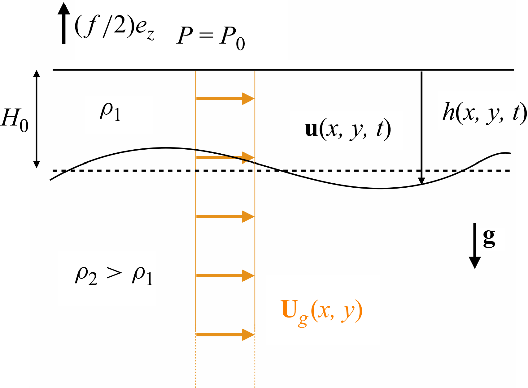


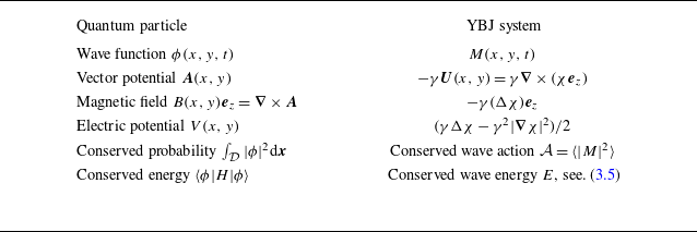


 Open access