


1. Introduction
Understanding the physics of droplet impact on a solid wall is an important practical problem, as well as being a source of scientific curiosity. Practical applications include inkjet printing (Yarin Reference Yarin2006), cooling (Yarin Reference Yarin2006; Sáenz et al. Reference Sáenz, Sefiane, Kim, Matar and Valluri2015) and crop spraying (Yarin Reference Yarin2006; Moghtadernejad, Lee & Jadidi Reference Moghtadernejad, Lee and Jadidi2020), while droplet impact on superhydrophobic surfaces has important de-icing applications in aviation and in power transmission (Khojasteh et al. Reference Khojasteh, Kazerooni, Salarian and Kamali2016). Droplet impact has been studied using experimental (Chandra & Avedisian Reference Chandra and Avedisian1991; Antonini, Amirfazli & Marengo Reference Antonini, Amirfazli and Marengo2012; Riboux & Gordillo Reference Riboux and Gordillo2014), theoretical (Roisman, Rioboo & Tropea Reference Roisman, Rioboo and Tropea2002; Gordillo, Riboux & Quintero Reference Gordillo, Riboux and Quintero2019) and computational (Fukai, Tanaka & Miyatake Reference Fukai, Tanaka and Miyatake1998; Gunjal, Ranade & Chaudhari Reference Gunjal, Ranade and Chaudhari2005; Eggers et al. Reference Eggers, Fontelos, Josserand and Zaleski2010) methods. The various impact regimes have been categorised as involving bounce, deposition or splash (Josserand & Thoroddsen Reference Josserand and Thoroddsen2016). Droplet splash can be further categorised as either prompt splash or corona splash. Bouncing and deposition depend on the wetting properties of the substrate. The regime which occurs also depends crucially on droplet’s Weber number ( ${\textit{We}}$
) and Reynolds number (
${\textit{We}}$
) and Reynolds number ( ${\textit{Re}}$
). For consistency with previous work (but going back to Eggers et al. (Reference Eggers, Fontelos, Josserand and Zaleski2010)), we use the definitions
${\textit{Re}}$
). For consistency with previous work (but going back to Eggers et al. (Reference Eggers, Fontelos, Josserand and Zaleski2010)), we use the definitions
 \begin{align} {\textit{Re}}=\frac {\rho U_0 R_0}{\mu },\qquad {\textit{We}}=\frac {\rho U_0^2 R_0}{\gamma }, \end{align}
where $\rho$
is the liquid density,
$\rho$
is the liquid density, $\mu$
is the liquid dynamic viscosity and
$\mu$
is the liquid dynamic viscosity and $\gamma$
is the surface tension. Also,
$\gamma$
is the surface tension. Also, $U_0$
is the droplet’s speed prior to impact and
$U_0$
is the droplet’s speed prior to impact and $R_0$
is the droplet radius prior to impact.
$R_0$
is the droplet radius prior to impact.
In this context, there is a splash parameter $K={\textit{We}}\sqrt {{\textit{Re}}}$
, which determines a threshold above which splash occurs (Mundo, Sommerfeld & Tropea Reference Mundo, Sommerfeld and Tropea1995). The threshold value is not universal (Marengo et al. Reference Marengo, Antonini, Roisman and Tropea2011), and different experiments have produced different values, a summary of which is provided in Moreira, Moita & Panao (Reference Moreira, Moita and Panao2010). The review by Josserand & Thoroddsen (Reference Josserand and Thoroddsen2016) states that ‘for impacts at
$K={\textit{We}}\sqrt {{\textit{Re}}}$
, which determines a threshold above which splash occurs (Mundo, Sommerfeld & Tropea Reference Mundo, Sommerfeld and Tropea1995). The threshold value is not universal (Marengo et al. Reference Marengo, Antonini, Roisman and Tropea2011), and different experiments have produced different values, a summary of which is provided in Moreira, Moita & Panao (Reference Moreira, Moita and Panao2010). The review by Josserand & Thoroddsen (Reference Josserand and Thoroddsen2016) states that ‘for impacts at $K$
exceeding
$K$
exceeding ${\sim}3000$
one can expect a splash’. Riboux & Gordillo (Reference Riboux and Gordillo2014) have recast the splash threshold in terms of powers of
${\sim}3000$
one can expect a splash’. Riboux & Gordillo (Reference Riboux and Gordillo2014) have recast the splash threshold in terms of powers of ${\textit{Re}}$
,
${\textit{Re}}$
, ${Oh}=\sqrt {\textit{We}}/{\textit{Re}}$
, and the gas–liquid viscosity ratio. The authors find good agreement between their theoretical model and experiments. Just below the splash threshold, and typically for
${Oh}=\sqrt {\textit{We}}/{\textit{Re}}$
, and the gas–liquid viscosity ratio. The authors find good agreement between their theoretical model and experiments. Just below the splash threshold, and typically for ${\textit{We}} \geq 10^2$
and
${\textit{We}} \geq 10^2$
and ${\textit{Re}} \geq 10^3$
(de Ruiter et al. Reference de, Jolet, Rachel and Stone2010), there is a ‘rim-lamella’ (RL) regime, in which the droplet flattens and spreads into an axisymmetric structure involving a lamella, with a thicker rim forming at the extremity. A key parameter which characterises the droplet impact in this regime is the maximum spreading radius, denoted here by
${\textit{Re}} \geq 10^3$
(de Ruiter et al. Reference de, Jolet, Rachel and Stone2010), there is a ‘rim-lamella’ (RL) regime, in which the droplet flattens and spreads into an axisymmetric structure involving a lamella, with a thicker rim forming at the extremity. A key parameter which characterises the droplet impact in this regime is the maximum spreading radius, denoted here by $\mathcal{R}_{\textit{max}}$
, and is governed by
$\mathcal{R}_{\textit{max}}$
, and is governed by ${\textit{We}}$
and
${\textit{We}}$
and ${\textit{Re}}$
. This quantity has applications in inkjet printing and forensic science (Josserand & Thoroddsen Reference Josserand and Thoroddsen2016). Even in this deposition regime, the presence of azimuthal instabilities which do not lead to topological transitions has been noted (Huang, Wan & Taslim Reference Huang, Wan and Taslim2018).
${\textit{Re}}$
. This quantity has applications in inkjet printing and forensic science (Josserand & Thoroddsen Reference Josserand and Thoroddsen2016). Even in this deposition regime, the presence of azimuthal instabilities which do not lead to topological transitions has been noted (Huang, Wan & Taslim Reference Huang, Wan and Taslim2018).
Certainly, droplet spreading is a three-dimensional phenomenon, exhibiting axisymmetry below the splash threshold. However, this paper focuses instead on cylindrical (quasi-two-dimensional) droplet impacts. Cylindrical droplets are unstable to the Rayleigh–Plateau instability, and cannot exist naturally over time scales greater than a characteristic breakup time $t_{\textit{breakup}}\sim [\rho R_0^3/\gamma ]^{1/2}$
(
$t_{\textit{breakup}}\sim [\rho R_0^3/\gamma ]^{1/2}$
( ${\lt}4\,\mathrm{ms}$
for a
${\lt}4\,\mathrm{ms}$
for a $1\,\mathrm{mm}$
-radius cylinder of water in air) (Chandrasekhar Reference Chandrasekhar1981). However, the present study may be indirectly applicable in certain experimental works, a summary of which is presented below.
$1\,\mathrm{mm}$
-radius cylinder of water in air) (Chandrasekhar Reference Chandrasekhar1981). However, the present study may be indirectly applicable in certain experimental works, a summary of which is presented below.
We mention in particular the paper by Néel et al. (Reference Néel, Lhuissier and Villermaux2020). There, the authors pierce a liquid sheet in two separate places, to form two holes in the sheet. The holes retract along their respective rims, with each rim rolling up into a toroidal shape. Arguably, the process is better described using a schematic diagram, which, for the purpose of maintaining focus in the introduction, is relegated to Appendix A. As the holes expand, their rims (the tori) approach one another and eventually collide. The minor radius of each torus is small compared with the size of the collision zone, meaning the collision is similar to a head-on collision of two liquid cylinders. The maximum spreading of the impacting tori scales as $\mathcal{R}_{\textit{max}}\sim {\textit{We}}$
, which we demonstrate below using the RL model to be a fundamentally two-dimensional (2-D) scaling behaviour.
$\mathcal{R}_{\textit{max}}\sim {\textit{We}}$
, which we demonstrate below using the RL model to be a fundamentally two-dimensional (2-D) scaling behaviour.
We mention also the work by Camus (Reference Camus1971), in which a cylindrical liquid droplet is generated by confining a liquid bridge between two parallel plates. Impact is achieved by projecting a third plate between the two spaced plates. Images of the resulting quasi-2-D droplet impacts are reproduced in the work by Field, Lesser & Dear (Reference Field, Lesser and Dear1985). This configuration enables precise observation of the internal dynamics (e.g. via schlieren imaging), while avoiding the refraction problems inherent in studies of spherical droplets (Field et al. Reference Field, Lesser and Dear1985). Although the work of Camus involves extremely high impact speeds (up to $70\,\mathrm{m}\,\mathrm{s}^{-1}$
) where compressibility effects are important, it does show how quasi-2-D impacts are realisable in the laboratory and are therefore a worthwhile subject for theoretical modelling.
$70\,\mathrm{m}\,\mathrm{s}^{-1}$
) where compressibility effects are important, it does show how quasi-2-D impacts are realisable in the laboratory and are therefore a worthwhile subject for theoretical modelling.
The same basic method of creating quasi-2-D droplets has been applied by Kärki et al. (Reference Kärki, Pääkkönen, Kyriakopoulos and Timonen2024). The paper also contains some investigations of droplet impact in two dimensions, albeit at very low impact speeds with ${\textit{We}}\ll 1$
– the opposite extreme to Camus (Reference Camus1971). Therefore, the present work addresses (albeit only theoretically) a missing regime not covered by the experiments. This observation comes with the caveat that the investigated quasi-2-D droplets are sustained between two plates, and thus, the presented model can only ever provide a partial representation of these experiments.
${\textit{We}}\ll 1$
– the opposite extreme to Camus (Reference Camus1971). Therefore, the present work addresses (albeit only theoretically) a missing regime not covered by the experiments. This observation comes with the caveat that the investigated quasi-2-D droplets are sustained between two plates, and thus, the presented model can only ever provide a partial representation of these experiments.
A further motivation for the study of 2-D RL models is to shed light on computational works. We mention the work by Tang, Adcock & Mostert (Reference Tang, Adcock and Mostert2024), in which the authors simulate the head-on collision of two liquid cylinders (equivalent to the impact of a liquid cylinder on a free-slip surface with contact angle $90^\circ$
). These simulations are performed in a full three-dimensional (3-D) geometry, and fingering is observed post collision, corresponding to an impact scenario above an effective splash threshold (e.g. figure 11
b). To understand the simulation results in depth, the authors introduce a 2-D RL model for the head-on collision of the two liquid cylinders. This particular model is a special case of the model in the present work. The theoretical bounds obtained herein can therefore be used to understand the scaling behaviour (with
$90^\circ$
). These simulations are performed in a full three-dimensional (3-D) geometry, and fingering is observed post collision, corresponding to an impact scenario above an effective splash threshold (e.g. figure 11
b). To understand the simulation results in depth, the authors introduce a 2-D RL model for the head-on collision of the two liquid cylinders. This particular model is a special case of the model in the present work. The theoretical bounds obtained herein can therefore be used to understand the scaling behaviour (with ${\textit{We}}$
) of this particular collision set-up. Appropriate schematic diagrams depicting both the experiment of Kärki et al. (Reference Kärki, Pääkkönen, Kyriakopoulos and Timonen2024) and the simulations of Tang et al. (Reference Tang, Adcock and Mostert2024) are provided in Appendix A.
${\textit{We}}$
) of this particular collision set-up. Appropriate schematic diagrams depicting both the experiment of Kärki et al. (Reference Kärki, Pääkkönen, Kyriakopoulos and Timonen2024) and the simulations of Tang et al. (Reference Tang, Adcock and Mostert2024) are provided in Appendix A.
We mention finally the wide range of previous computational studies on 2-D droplet impact, for instance Ding, Spelt & Shu (Reference Ding, Spelt and Shu2007), Shin & Juric (Reference Shin and Juric2009), Gupta & Kumar (Reference Gupta and Kumar2011), Wu & Cao (Reference Wu and Cao2017), Wu et al. (Reference Wu, Gui, Yang, Tu and Jiang2021) and Rafi, Haque & Ahmed (Reference Rafi, Haque and Ahmed2022). By providing a rigorous method to estimate the spreading radius, the present theoretical analysis provides insights into these studies.
In Ó Náraigh & Mairal (Reference Ó Náraigh and Mairal2023), a 2-D energy-budget analysis of droplet impact is proposed. This allows one to estimate the maximum spreading radius, written in dimensionless terms as $\beta _{\textit{max}}=\mathcal{R}_{\textit{max}}/R_0$
. By balancing the energy before impact and at maximum spreading, the following correlation is obtained:
$\beta _{\textit{max}}=\mathcal{R}_{\textit{max}}/R_0$
. By balancing the energy before impact and at maximum spreading, the following correlation is obtained:
 \begin{align} \underbrace {1}_{{\overset {\text{Pre-impact}}{\scriptscriptstyle \text{kinetic energy}}}}+\underbrace {\frac {4}{\textit{We}}}_{\overset {\text{Pre-impact}}{\scriptscriptstyle \text{surface energy}}} &= \underbrace {\frac {2}{\pi {\textit{We}}}\left [2\beta _{\textit{max}}\left (1-\cos \vartheta \right )+ \frac {\pi }{\beta _{\textit{max}}}\right ]}_{\overset {\text{Surface energy}}{\scriptscriptstyle \text{at maximum spreading}}} \nonumber \\&\quad +\underbrace {\frac {2}{\pi }\frac {2a}{\sqrt {{\textit{Re}}}}\beta _{\textit{max}}\sqrt {\beta _{\textit{max}}-1}}_{\overset {\text{Viscous dissipation}}{\scriptscriptstyle \text{in the boundary layer}}}+\underbrace {b}_{\text{Head loss}} \! . \end{align}
Hence, (1.2) is an energy balance made dimensionless on the kinetic energy density $(1/2)\rho U_0^2$
. Also,
$(1/2)\rho U_0^2$
. Also, $\vartheta$
is an appropriate contact angle, usually taken to be the advancing contact angle (for a discussion on this, see Wang et al. (Reference Wang, Yang, Wang, Zhu and Fang2019)). The `head loss’ term in (1.2) is a key term which reflects energy dissipation due to internal flows which develop in the RL structure and which are otherwise not included in a simple energy balance. The head loss can be modelled as a simple fraction of the initial kinetic energy (Wildeman et al. Reference Wildeman, Visser, Sun and Lohse2016). A theoretical justification for this is given in Villermaux & Bossa (Reference Villermaux and Bossa2011). In this way, (1.2) contains two free parameters,
$\vartheta$
is an appropriate contact angle, usually taken to be the advancing contact angle (for a discussion on this, see Wang et al. (Reference Wang, Yang, Wang, Zhu and Fang2019)). The `head loss’ term in (1.2) is a key term which reflects energy dissipation due to internal flows which develop in the RL structure and which are otherwise not included in a simple energy balance. The head loss can be modelled as a simple fraction of the initial kinetic energy (Wildeman et al. Reference Wildeman, Visser, Sun and Lohse2016). A theoretical justification for this is given in Villermaux & Bossa (Reference Villermaux and Bossa2011). In this way, (1.2) contains two free parameters, $a$
and
$a$
and $b$
, which have been fitted to the data emanating from numerical simulations (Ó Náraigh & Mairal Reference Ó Náraigh and Mairal2023).
$b$
, which have been fitted to the data emanating from numerical simulations (Ó Náraigh & Mairal Reference Ó Náraigh and Mairal2023).
Equation (1.2) has some important asymptotic limits:
-
(i) inviscid limit: for ${\textit{Re}}\rightarrow \infty$
, (1.2) reduces to(1.3)with exact solution
\begin{align} \frac {\pi }{2}(1-b){\textit{We}}+2\pi =\left [2\beta _{\textit{max}}(1-\cos \vartheta )+\frac {\pi }{\beta _{\textit{max}}}\right ]\!, \end{align}
(1.4)For
\begin{align} \beta _{\textit{max}}=\frac {\omega +\sqrt {\omega ^2-8\pi (1-\cos \vartheta )}}{4(1-\cos \vartheta )},\qquad \omega =\frac {\pi }{2}(1-b){\textit{We}}+2\pi . \end{align}
${\textit{We}}$
large but finite, this further reduces to(1.5)The equivalent scaling behaviour for 3-D axisymmetric droplets is (Wildeman et al. Reference Wildeman, Visser, Sun and Lohse2016)
\begin{align} \beta _{\textit{max}}\approx \frac {{\textit{We}}\,\pi (1-b)}{4(1-\cos \vartheta )}. \end{align}
(1.6)hence,
\begin{align} \beta _{\textit{max}}\approx \sqrt {\frac {4}{1-\cos \vartheta }\left [\dfrac {1}{12}(1-b){\textit{We}}+1\right ]}, \end{align}
$\beta _{\textit{max}}\sim {\textit{We}}$
for 2-D Cartesian droplets and
$\beta _{\textit{max}}\sim {\textit{We}}^{1/2}$
for 3-D axisymmetric droplets;
${\textit{Re}}\rightarrow \infty$
, (1.2) reduces to(1.3)with exact solution
\begin{align} \frac {\pi }{2}(1-b){\textit{We}}+2\pi =\left [2\beta _{\textit{max}}(1-\cos \vartheta )+\frac {\pi }{\beta _{\textit{max}}}\right ]\!, \end{align}
(1.4)For
\begin{align} \beta _{\textit{max}}=\frac {\omega +\sqrt {\omega ^2-8\pi (1-\cos \vartheta )}}{4(1-\cos \vartheta )},\qquad \omega =\frac {\pi }{2}(1-b){\textit{We}}+2\pi . \end{align}
${\textit{We}}$
large but finite, this further reduces to(1.5)The equivalent scaling behaviour for 3-D axisymmetric droplets is (Wildeman et al. Reference Wildeman, Visser, Sun and Lohse2016)
\begin{align} \beta _{\textit{max}}\approx \frac {{\textit{We}}\,\pi (1-b)}{4(1-\cos \vartheta )}. \end{align}
(1.6)hence,
\begin{align} \beta _{\textit{max}}\approx \sqrt {\frac {4}{1-\cos \vartheta }\left [\dfrac {1}{12}(1-b){\textit{We}}+1\right ]}, \end{align}
$\beta _{\textit{max}}\sim {\textit{We}}$
for 2-D Cartesian droplets and
$\beta _{\textit{max}}\sim {\textit{We}}^{1/2}$
for 3-D axisymmetric droplets;
-
(ii) finite viscosity, large Weber number: for
${\textit{We}}\rightarrow \infty$
(1.2) reduces to(1.7)For
\begin{align} \frac {\pi }{2}(1-b)\approx \frac {2a}{\sqrt {{\textit{Re}}}}\beta _{\textit{max}}\sqrt {\beta _{\textit{max}}-1}. \end{align}
${\textit{Re}}$
large but finite, this gives
$\beta _{\textit{max}}\sim {\textit{Re}}^{1/3}$
for 2-D Cartesian droplets. The corresponding result for 3-D axisymmetric droplets is
$\beta _{\textit{max}}\sim {\textit{Re}}^{1/5}$
.


In the 3-D axisymmetric case, a RL model provides an alternative method for estimating the maximum spreading radius for 3-D axisymmetric droplets. The RL model is pertinent when the droplet spreads to form a RL structure (specifically, ${\textit{We}} \gtrsim 10^2$
,
${\textit{We}} \gtrsim 10^2$
, ${\textit{Re}} \gtrsim 10^3$
and below the splash threshold
${\textit{Re}} \gtrsim 10^3$
and below the splash threshold $K={\textit{We}}\sqrt {{\textit{Re}}}\lesssim 10^3-10^4$
). In a previous set of papers by Amirfazli et al. (Reference Amirfazli, Bustamante, Hu and Ó Náraigh2024) and Bustamante & Ó Náraigh (Reference Bustamante and Ó Náraigh2025), one of the present authors (with co-authors) was able to place rigorous bounds on the maximum spreading radius for 3-D axisymmetric droplets ((1.3), Bustamante & Ó Náraigh (Reference Bustamante and Ó Náraigh2025)). The bounds were derived by first formulating a RL model and then analysing the resulting set of ordinary differential equations using differential inequalities, in particular, Gronwall’s inequality (Doering & Gibbon Reference Doering and Gibbon1995). The bounds are found to be consistent with the correlation given by Roisman (Reference Roisman2009), stated here for a Reynolds number and a Weber number based on droplet radius (not diameter)
$K={\textit{We}}\sqrt {{\textit{Re}}}\lesssim 10^3-10^4$
). In a previous set of papers by Amirfazli et al. (Reference Amirfazli, Bustamante, Hu and Ó Náraigh2024) and Bustamante & Ó Náraigh (Reference Bustamante and Ó Náraigh2025), one of the present authors (with co-authors) was able to place rigorous bounds on the maximum spreading radius for 3-D axisymmetric droplets ((1.3), Bustamante & Ó Náraigh (Reference Bustamante and Ó Náraigh2025)). The bounds were derived by first formulating a RL model and then analysing the resulting set of ordinary differential equations using differential inequalities, in particular, Gronwall’s inequality (Doering & Gibbon Reference Doering and Gibbon1995). The bounds are found to be consistent with the correlation given by Roisman (Reference Roisman2009), stated here for a Reynolds number and a Weber number based on droplet radius (not diameter)
 \begin{align} \beta _{\textit{max}}=1.00{\textit{Re}}^{1/5}-0.37{\textit{Re}}^{2/5}{\textit{We}}^{-1/2},\qquad \text{(3-D axisymmetric)}. \end{align}
The correlation (1.8) has been validated extensively via numerical simulation (Wildeman et al. Reference Wildeman, Visser, Sun and Lohse2016) and experimental measurements. For completeness, we mention also the correlation due to Laan et al. (Reference Laan, De, Karla, Bartolo, Josserand and Bonn2014), which gives
 \begin{align} \beta _{\textit{max}}=a_0{\textit{Re}}^{1/5}\frac {P^{1/2}}{a_1+P^{1/2}}, \end{align}
a relationship also used in bloodstain pattern analysis (Laan et al. Reference Laan, de, Karla, Slenter, Wilhelm, Jermy and Bonn2015). Here, $P={\textit{WeRe}}^{-2/5}$
and
$P={\textit{WeRe}}^{-2/5}$
and $a_0$
and
$a_0$
and $a_1$
are empirical coefficients. Equation (1.9) reverts to (1.8) in the limit of large
$a_1$
are empirical coefficients. Equation (1.9) reverts to (1.8) in the limit of large $P$
. Such correlations have now been identified as limiting regimes within a unified framework by Sanjay & Lohse (Reference Sanjay and Lohse2025), while the effect of non-Newtonian rheology on the correlation has also been quantified by Mobaseri, Kumar & Cheng (Reference Mobaseri, Kumar and Cheng2025). Hence, based on the theory of Sanjay & Lohse (Reference Sanjay and Lohse2025), (1.8) is valid below the splash threshold at large
$P$
. Such correlations have now been identified as limiting regimes within a unified framework by Sanjay & Lohse (Reference Sanjay and Lohse2025), while the effect of non-Newtonian rheology on the correlation has also been quantified by Mobaseri, Kumar & Cheng (Reference Mobaseri, Kumar and Cheng2025). Hence, based on the theory of Sanjay & Lohse (Reference Sanjay and Lohse2025), (1.8) is valid below the splash threshold at large $P$
and low
$P$
and low $\textit{Oh}$
.
$\textit{Oh}$
.
1.1. Aim of the paper
The main aim of the present work is to establish a result analogous to (1.8) for 2-D droplets. For this purpose, we formulate a RL model for 2-D droplets. Within the framework of the RL model, we show
 \begin{align} k_1 {\textit{Re}}^{1/3}-k_2 {\textit{Re}}^{1/2}{\textit{We}}^{-1/2}(1-\cos \vartheta _a)^{1/2} \leq \beta _{\textit{max}}\leq k_1 {\textit{Re}}^{1/3}, \qquad \text{(2-D Cartesian)}, \end{align}
where $k_1$
and
$k_1$
and $k_2$
are constants to be determined, and
$k_2$
are constants to be determined, and $\vartheta _a$
is the advancing contact angle. We verify the bounds (1.10) using computational fluid dynamics simulations of droplet impact. We use the volume of fluid (VOF) method to capture the interface and hence to model the multiphase flow.
$\vartheta _a$
is the advancing contact angle. We verify the bounds (1.10) using computational fluid dynamics simulations of droplet impact. We use the volume of fluid (VOF) method to capture the interface and hence to model the multiphase flow.
A key motivation for studying the 2-D case is that the RL model in two dimensions is much simpler than in three dimensions. This makes the analysis more tractable. As a by-product of this analysis, we find that the RL model in the 2-D inviscid case is exactly solvable in terms of polynomials and square roots. This enables us to obtain an analytical expression confirming the scaling behaviour $\beta _{\textit{max}}\sim {\textit{We}}$
.
$\beta _{\textit{max}}\sim {\textit{We}}$
.
1.2. Plan of the paper
In § 2 we derive the RL model from first principles. The result is a set of coupled ordinary differential equations for the rim area $V$
, the greatest extent of the lamella
$V$
, the greatest extent of the lamella $R$
and the lamella height
$R$
and the lamella height $h$
. In § 3 we examine the inviscid limit of the model, where we derive a closed-form expression for
$h$
. In § 3 we examine the inviscid limit of the model, where we derive a closed-form expression for $R(t)$
, the variation of
$R(t)$
, the variation of $R$
with respect to time. Crucially, we find a closed-form expression for the maximum value of
$R$
with respect to time. Crucially, we find a closed-form expression for the maximum value of $R(t)$
,
$R(t)$
, $R_{\textit{max}}$
and show that it scales linearly with Weber number, a result consistent with the energy-budget analysis (1.5). In § 4 we extend the analysis to the viscous case. In this case, an exact closed-form solution is not possible; however, we use an analysis of the RL model based on Gronwall’s inequality to establish the bounds (1.10). In § 5 we validate the bounds using numerical simulations of 2-D droplet impact within the framework of the VOF method. Discussion and concluding remarks are presented in § 6. We emphasise that, in this paper, we use the symbol
$R_{\textit{max}}$
and show that it scales linearly with Weber number, a result consistent with the energy-budget analysis (1.5). In § 4 we extend the analysis to the viscous case. In this case, an exact closed-form solution is not possible; however, we use an analysis of the RL model based on Gronwall’s inequality to establish the bounds (1.10). In § 5 we validate the bounds using numerical simulations of 2-D droplet impact within the framework of the VOF method. Discussion and concluding remarks are presented in § 6. We emphasise that, in this paper, we use the symbol $V$
for rim area, to emphasise the similarity of theoretical model with previous work on 3-D axisymmetric droplets, where
$V$
for rim area, to emphasise the similarity of theoretical model with previous work on 3-D axisymmetric droplets, where $V$
was used to denote a rim volume.
$V$
was used to denote a rim volume.
2. Mathematical model
We introduce a RL model for 2-D droplets, based on the analogous one for 3-D axisymmetric droplets given by Bustamante & Ó Náraigh (Reference Bustamante and Ó Náraigh2025) (but see also Eggers et al. (Reference Eggers, Fontelos, Josserand and Zaleski2010) and Gordillo et al. (Reference Gordillo, Riboux and Quintero2019)). The schematic diagram is presented in figure 1. The diagram shows the development of the RL structure at a time $\tau$
after the initial droplet impact. A hyperbolic flow arises from the droplet impact after a characteristic time
$\tau$
after the initial droplet impact. A hyperbolic flow arises from the droplet impact after a characteristic time $t_0$
, the horizontal component of which drives the flow in the lamella. Air resistance and compressibility are neglected in the derivations, which is appropriate for the range of Reynolds and Weber numbers considered in the work, together with the implied droplet length scale
$t_0$
, the horizontal component of which drives the flow in the lamella. Air resistance and compressibility are neglected in the derivations, which is appropriate for the range of Reynolds and Weber numbers considered in the work, together with the implied droplet length scale $R_0=O\,(\mathrm{mm})$
. We work through the different elements of the model, starting with the flow in the lamella.
$R_0=O\,(\mathrm{mm})$
. We work through the different elements of the model, starting with the flow in the lamella.
Schematic diagram showing the cross-section of a 2-D RL structure. Dashed curved line: true lamella height $h(x,t)=(t+t_0)^{-1}f[(x/(t+t_0)]+h_{\textit{PI}}(t)$
, as given by (2.6). Dashed straight line: the remote asymptotic approximation
$h(x,t)=(t+t_0)^{-1}f[(x/(t+t_0)]+h_{\textit{PI}}(t)$
, as given by (2.6). Dashed straight line: the remote asymptotic approximation $h(x,t)=h_{\textit{init}}(\tau +t_0)/(t+t_0)+h_{\textit{PI}}(t)$
.
$h(x,t)=h_{\textit{init}}(\tau +t_0)/(t+t_0)+h_{\textit{PI}}(t)$
.

We emphasise that in this work, we use a RL model to place bounds on the maximum value of $R$
. However, from figure 1, it can be seen that
$R$
. However, from figure 1, it can be seen that $\mathcal{R}_{\textit{max}}=R+2a$
, where
$\mathcal{R}_{\textit{max}}=R+2a$
, where $\mathcal{R}_{\textit{max}}$
is the quantity of interest. However, in § 4 we will demonstrate that
$\mathcal{R}_{\textit{max}}$
is the quantity of interest. However, in § 4 we will demonstrate that $2a$
is negligibly small compared with
$2a$
is negligibly small compared with $R$
, and hence can be ignored.
$R$
, and hence can be ignored.
2.1. Flow in the lamella
The horizontal flow far from the substrate is denoted by $u_{\textit{outer}}$
(the outer flow). Similar to the 3-D axisymmetric case, this is assumed to be a hyperbolic flow and is given (in 2-D Cartesian coordinates) by the expression
$u_{\textit{outer}}$
(the outer flow). Similar to the 3-D axisymmetric case, this is assumed to be a hyperbolic flow and is given (in 2-D Cartesian coordinates) by the expression
 \begin{align} u_{\textit{outer}}(x,t)=\frac {x}{t+t_0}, \end{align}
where $t_0$
is a model parameter which describes the onset time of the flow, prior to the formation of the RL structure. The assumption of this hyperbolic flow profile in the lamella is justified by earlier simulations of 2-D droplet impact (Ó Náraigh & Mairal Reference Ó Náraigh and Mairal2023).
$t_0$
is a model parameter which describes the onset time of the flow, prior to the formation of the RL structure. The assumption of this hyperbolic flow profile in the lamella is justified by earlier simulations of 2-D droplet impact (Ó Náraigh & Mairal Reference Ó Náraigh and Mairal2023).
A boundary layer forms close to the substrate, in which the fluid velocity transitions from $u_{\textit{outer}}$
to zero, across a distance
$u_{\textit{outer}}$
to zero, across a distance $h_{bl}$
, the boundary-layer thickness. From boundary-layer theory (White et al. Reference Frank2011), the boundary-layer thickness scales as
$h_{bl}$
, the boundary-layer thickness. From boundary-layer theory (White et al. Reference Frank2011), the boundary-layer thickness scales as $h_{bl}\propto \sqrt {\nu x/u_{\textit{outer}}}$
, where
$h_{bl}\propto \sqrt {\nu x/u_{\textit{outer}}}$
, where $\nu =\mu /\rho$
is the kinematic viscosity of the liquid. Given the functional form of
$\nu =\mu /\rho$
is the kinematic viscosity of the liquid. Given the functional form of $u_{\textit{outer}}$
, the
$u_{\textit{outer}}$
, the $x$
-dependence cancels out, to give
$x$
-dependence cancels out, to give $h_{bl}\propto \sqrt {\nu (t+t_0)}$
. We allow for an additional degree of freedom in the problem by taking
$h_{bl}\propto \sqrt {\nu (t+t_0)}$
. We allow for an additional degree of freedom in the problem by taking $h_{bl}\propto \sqrt {\nu (t+t_1)}$
, where
$h_{bl}\propto \sqrt {\nu (t+t_1)}$
, where $t_1$
describes the time of formation of the boundary layer (Eggers et al. Reference Eggers, Fontelos, Josserand and Zaleski2010). Following boundary-layer theory (White et al. Reference Frank2011), we describe the vertical variation of the flow using a transition function, such that
$t_1$
describes the time of formation of the boundary layer (Eggers et al. Reference Eggers, Fontelos, Josserand and Zaleski2010). Following boundary-layer theory (White et al. Reference Frank2011), we describe the vertical variation of the flow using a transition function, such that
 \begin{align} u(x,z,t)=u_{\textit{outer}}(x,t)F(z), \end{align}
where $F(z=0)=0$
and
$F(z=0)=0$
and $F(z)=1$
for
$F(z)=1$
for $z\geq h_{bl}$
. For simplicity, and following Bustamante & Ó Náraigh (Reference Bustamante and Ó Náraigh2025) and Eggers et al. (Reference Eggers, Fontelos, Josserand and Zaleski2010) for the 3-D axisymmetric case, we use a step function for the transition function, such that
$z\geq h_{bl}$
. For simplicity, and following Bustamante & Ó Náraigh (Reference Bustamante and Ó Náraigh2025) and Eggers et al. (Reference Eggers, Fontelos, Josserand and Zaleski2010) for the 3-D axisymmetric case, we use a step function for the transition function, such that
 \begin{align} F(z)=\begin{cases} 0,& z\lt h_{bl},\\ 1,& z\gt h_{bl}.\end{cases} \end{align}
We have used the notation $u(x,z,t)$
for the flow in the horizontal direction; the corresponding flow in the vertical direction is denoted by
$u(x,z,t)$
for the flow in the horizontal direction; the corresponding flow in the vertical direction is denoted by $w(x,z,t)$
. We use the incompressibility condition
$w(x,z,t)$
. We use the incompressibility condition $\partial _x u+\partial _z w=0$
to obtain an expression for
$\partial _x u+\partial _z w=0$
to obtain an expression for $w(x,z,t)$
 \begin{align} w(x,z,t)=\begin{cases} 0,& z\lt h_{bl},\\ -\dfrac {z-h_{bl}}{t+t_0},&z\gt h_{bl}.\end{cases} \end{align}
2.2. Lamella height
To model the lamella height $h(x,t)$
, we assume the kinematic condition, such that the interface
$h(x,t)$
, we assume the kinematic condition, such that the interface $h(x,t)$
moves with the flow. Hence, the height of the lamella
$h(x,t)$
moves with the flow. Hence, the height of the lamella $h(x,t)$
satisfies
$h(x,t)$
satisfies
 \begin{align} \frac {\partial h}{\partial t}+u |_{z=h}\frac {\partial h}{\partial x}=w |_{z=h}. \end{align}
In the remainder of this section, we assume we are in phase 1 of the motion, such that $h(R,t)\gt h_{bl}$
, and such that
$h(R,t)\gt h_{bl}$
, and such that $(u,w)_{z=h}\neq 0$
. We discuss phase 2 of the motion, wherein
$(u,w)_{z=h}\neq 0$
. We discuss phase 2 of the motion, wherein $h(R,t)$
reaches a limiting value set by the boundary layer, and
$h(R,t)$
reaches a limiting value set by the boundary layer, and $(u,w)_{z=h}=0$
in § 4. Thus, (2.5) becomes
$(u,w)_{z=h}=0$
in § 4. Thus, (2.5) becomes
 \begin{align} \frac {\partial h}{\partial t}+\frac {x}{t+t_0}\frac {\partial h}{\partial x}=w |_{z=h}=-\frac {h-h_{bl}}{t+t_0}. \end{align}
Equation (2.6) has an exact solution (valid in phase 1) by the method of characteristics
 \begin{align} h(x,t)=\frac {\tau +t_0}{t+t_0}f \!\left (x\frac {\tau +t_0}{t+t_0}\right )+ \underbrace {\frac {2}{3}\left [h_{bl}(t)\frac {t+t_1}{t+t_0}-h_{bl}(\tau )\frac {\tau +t_1}{t+t_0}\right ]}_{=h_{\textit{PI}}(t)}\qquad t\geq \tau , \end{align}
where $f$
is set by the initial conditions. At late times,
$f$
is set by the initial conditions. At late times, $f$
is taken to be a constant function, which is the so-called remote asymptotic solution (Roisman Reference Roisman2009). Here, we use the parameter
$f$
is taken to be a constant function, which is the so-called remote asymptotic solution (Roisman Reference Roisman2009). Here, we use the parameter $\tau$
to denote the initial time
$\tau$
to denote the initial time $t=\tau$
at which point the RL structure seen in figure 1 forms. As in the 3-D axisymmetric case (Marengo et al. Reference Marengo, Antonini, Roisman and Tropea2011), the contribution
$t=\tau$
at which point the RL structure seen in figure 1 forms. As in the 3-D axisymmetric case (Marengo et al. Reference Marengo, Antonini, Roisman and Tropea2011), the contribution $h_{\textit{PI}}(t)$
is the viscous correction, it is positive definite and, as such, represents a thickening of the lamella compared with the inviscid scenario.
$h_{\textit{PI}}(t)$
is the viscous correction, it is positive definite and, as such, represents a thickening of the lamella compared with the inviscid scenario.
2.3. Mass conservation
We derive an Ordinary Differential Equation (ODE) for the volume of the rim in what follows. We omit the redundant dimension out of the plane of the page, which carries with it a factor of $\lambda$
, this being the length of the idealised cylindrical droplet. Hence, we work with the rim area
$\lambda$
, this being the length of the idealised cylindrical droplet. Hence, we work with the rim area $V$
, the lamella area
$V$
, the lamella area $2\int _0^R \mathrm{d} x\int _0^{h(x,t)}\mathrm{d} z$
and the total area
$2\int _0^R \mathrm{d} x\int _0^{h(x,t)}\mathrm{d} z$
and the total area $V_{\textit{tot}}$
, such that
$V_{\textit{tot}}$
, such that
 \begin{align} V_{\textit{tot}}=V+2\int _0^R \mathrm{d} x\int _0^{h(x,t)}\mathrm{d} z. \end{align}
We use $\mathrm{d} V_{\textit{tot}}/\mathrm{d} t=0$
and (2.6) to get
$\mathrm{d} V_{\textit{tot}}/\mathrm{d} t=0$
and (2.6) to get
 \begin{align} \frac {\mathrm{d} V}{\mathrm{d} t}=2 \!\left [\frac {R}{t+t_0}\left (1-\frac {h_{bl}}{h}\right )-\dot R\right ]h, \end{align}
where $R$
denotes the greatest extent of the lamella at time
$R$
denotes the greatest extent of the lamella at time $t$
, and where we henceforth use the simplified notation
$t$
, and where we henceforth use the simplified notation
 \begin{align} h\equiv h(t)\equiv h(R,t). \end{align}
By mass conservation, (2.9) has exact solution
 \begin{align} V=V_{\textit{tot}}-2g \! \left (\!R\frac {\tau +t_0}{t+t_0}\right )-2 \! \left (\!R\frac {\tau +t_0}{t+t_0}\right ) \! h_{\textit{PI}}(t), \end{align}
where $g(s)=\int _0^s f\!(s)\,\mathrm{d} s$
.
$g(s)=\int _0^s f\!(s)\,\mathrm{d} s$
.
2.4. Momentum
In a similar way, we derive an ODE for the momentum of the rim. We work with one half of the rim momentum $P$
, and one half of the lamella momentum
$P$
, and one half of the lamella momentum $\rho \int _0^R \mathrm{d} x\int _0^{h(x,t)}\mathrm{d} z$
, such that the total momentum in (say) the right-hand half of the RL structure in figure 1 is
$\rho \int _0^R \mathrm{d} x\int _0^{h(x,t)}\mathrm{d} z$
, such that the total momentum in (say) the right-hand half of the RL structure in figure 1 is
 \begin{align} P_{\textit{tot}}=P+\rho \lambda \int _0^R \mathrm{d} x\int _0^h u \,\mathrm{d} z, \end{align}
where again, $\lambda$
is the length of the idealised cylindrical droplet in the plane of the page. When
$\lambda$
is the length of the idealised cylindrical droplet in the plane of the page. When $h\gt h_{bl}$
(phase 1) this becomes
$h\gt h_{bl}$
(phase 1) this becomes
 \begin{align} P_{\textit{tot}}=P+\underbrace {\rho \lambda \int _0^R \frac {x}{t+t_0}\left [h(x,t)-h_{bl}(t)\right ]\mathrm{d} x}_{=P_{\textit{lam}}}. \end{align}
By direct differentiation, we have
 \begin{align} \frac {\mathrm{d} P_{\textit{lam}}}{\mathrm{d} t} =\rho \lambda \left [\frac {R}{t+t_0}\left [h(R,t)-h_{bl}(t)\right ]\left (\dot R-\frac {R}{t+t_0}\right )-\dfrac {1}{4}\frac {h_{bl} R^2}{(t+t_0)(t+t_1)}\right ]\!. \end{align}
By Newton’s second law, we have
 \begin{align} \frac {\mathrm{d} P_{\textit{tot}}}{\mathrm{d} t}=F_{\textit{ext}}=-\lambda \gamma (1-\cos \vartheta _a). \end{align}
Here, $\vartheta _a$
is the advancing contact angle, assumed for the present purposes to be constant. Hence, combining (2.14) and (2.15) and using
$\vartheta _a$
is the advancing contact angle, assumed for the present purposes to be constant. Hence, combining (2.14) and (2.15) and using $h\equiv h(R,t)$
we have
$h\equiv h(R,t)$
we have
 \begin{align} -\lambda \gamma (1-\cos \vartheta _a)-\frac {R}{t+t_0}\rho \lambda \left [h-h_{bl}(t)\right ]\left (\dot R-\frac {R}{t+t_0}\right )+\frac {1}{4}\frac {\rho \lambda h_{bl} R^2}{(t+t_0)(t+t_1)}=\frac {\mathrm{d} P}{\mathrm{d} t}. \end{align}
We use $\mathrm{d} P/\mathrm{d} t=\rho \lambda U (\mathrm{d} V_{1/2}/\mathrm{d} t)+\rho \lambda V_{1/2}(\mathrm{d} U/\mathrm{d} t)$
(
$\mathrm{d} P/\mathrm{d} t=\rho \lambda U (\mathrm{d} V_{1/2}/\mathrm{d} t)+\rho \lambda V_{1/2}(\mathrm{d} U/\mathrm{d} t)$
( $V_{1/2}$
is half the rim area) and
$V_{1/2}$
is half the rim area) and $U\equiv \dot R$
to re-write the momentum equation in a final form
$U\equiv \dot R$
to re-write the momentum equation in a final form
 \begin{align} \rho V\frac {\mathrm{d} U}{\mathrm{d} t}=2\rho \big \{\left [h-h_{bl}(t)\right ]\left (u_0-U\right )^2+U^2h_{bl}\big \}+\frac {1}{2}\frac {\rho h_{bl} R^2}{(t+t_0)(t+t_1)}-2\gamma (1-\cos \vartheta _a). \end{align}
Here, we have divided out by the redundant length scale $\lambda$
, and we have introduced the notation
$\lambda$
, and we have introduced the notation $u_0\equiv R/(t+t_0)$
.
$u_0\equiv R/(t+t_0)$
.
2.5. Summary of the model equations
We gather up the model equations here in one place. We emphasise that the equations are for phase 1 of the motion, wherein $h(t)\gt h_{bl}(t)$
 \begin{align} \frac {\mathrm{d} V}{\mathrm{d} t}&=2\big [ u_0\left (h-h_{bl}\right )- \textit{Uh}\big ], \\[-9pt] \nonumber \end{align}
 \begin{align} \frac {\mathrm{d} R}{\mathrm{d} t}&=U, \\[-9pt] \nonumber \end{align}
 \begin{align} V\frac {\mathrm{d} U}{\mathrm{d} t}&=2\big [(u_0-U)^2\left (h-h_{bl}\right )+U^2h_{bl}\big ]\nonumber \\&\quad +\frac {1}{2}\frac {h_{bl} R^2}{(t+t_0)(t+t_1)}-2\frac {\gamma }{\rho }(1-\cos \vartheta _a), \\[9pt] \nonumber \end{align}
where $h$
is given by (2.10), and
$h$
is given by (2.10), and $u_0=R/(t+t_0)$
. We analyse (2.18) in the following sections.
$u_0=R/(t+t_0)$
. We analyse (2.18) in the following sections.
3. Inviscid case
In this section we look at the RL model (2.18) in the inviscid case, which can be obtained by shrinking the boundary layer $h_{bl}$
to zero. Hence, the model simplifies
$h_{bl}$
to zero. Hence, the model simplifies
 \begin{align} \frac {\mathrm{d} V}{\mathrm{d} t}&=2 (u_0-U)h, \\[-9pt] \nonumber \end{align}
 \begin{align} \frac {\mathrm{d} R}{\mathrm{d} t}&=U, \\[-9pt] \nonumber \end{align}
 \begin{align} V\frac {\mathrm{d} U}{\mathrm{d} t}&=2 (u_0-U)^2h-{\frac {2\gamma }{\rho }}(1-\cos \vartheta _a). \\[9pt] \nonumber \end{align}
The corresponding RL model in the 3-D axisymmetric case has a geometric factor of $2\pi R$
on the right-hand side of both the mass-conservation equation and the momentum equation (Amirfazli et al. Reference Amirfazli, Bustamante, Hu and Ó Náraigh2024). The fact that this factor does not occur in 2-D RL model (3.1) means that it has an exact solution, which we present here.
$2\pi R$
on the right-hand side of both the mass-conservation equation and the momentum equation (Amirfazli et al. Reference Amirfazli, Bustamante, Hu and Ó Náraigh2024). The fact that this factor does not occur in 2-D RL model (3.1) means that it has an exact solution, which we present here.
3.1. Exact solution
As in the 3-D axisymmetric model, we introduce the velocity defect $\varDelta =u_0-U$
. (3.1) can then be recast in terms of an ODE for
$\varDelta =u_0-U$
. (3.1) can then be recast in terms of an ODE for $\varDelta$
 \begin{align} \frac {\mathrm{d} \Delta }{\mathrm{d} t}+\frac {\varDelta }{t+t_0}=-\frac {2h}{V}\big (\varDelta ^2-c^2\big ), \end{align}
where
 \begin{align} c= \sqrt { \frac {\gamma }{\rho h}(1-\cos \vartheta _a)} \end{align}
is the Taylor–Culick speed ( $c$
is time-dependent, through
$c$
is time-dependent, through $h$
). We further recast (3.2) as an ODE for
$h$
). We further recast (3.2) as an ODE for $V \kern-1pt \Delta$
 \begin{align} \frac {\mathrm{d} }{\mathrm{d} t}(V\kern-1.5pt\Delta )+\frac {V \kern-1pt \Delta }{t+t_0}=2hc^2=2(\gamma /\rho )(1-\cos \vartheta _a). \end{align}
Thus, there is an exact solution for $V \kern-1pt \Delta$
 \begin{align} V \kern-1pt \Delta =V_{\textit{init}}\varDelta _{\textit{init}}\left (\frac {\tau +t_0}{t+t_0}\right )+\frac {\gamma }{\rho }\left (1-\cos \vartheta _a\right )\left [t+t_0-\frac {(\tau +t_0)^2}{t+t_0}\right ]\!, \end{align}
where $V_{\textit{init}}$
denotes the initial condition, i.e.
$V_{\textit{init}}$
denotes the initial condition, i.e. $V$
evaluated at
$V$
evaluated at $t=\tau$
, and similarly for
$t=\tau$
, and similarly for $\varDelta _{\textit{init}}$
. We recall the definition of
$\varDelta _{\textit{init}}$
. We recall the definition of $\varDelta$
, to obtain
$\varDelta$
, to obtain
 \begin{align} \frac {\mathrm{d} R}{\mathrm{d} t}-\frac {R}{t+t_0}=-\frac {V_{\textit{init}}}{V}\varDelta _{\textit{init}}\left (\frac {\tau +t_0}{t+t_0}\right )-\frac {\gamma }{\rho }\frac {\left (1-\cos \vartheta _a\right )}{V}\left [t+t_0-\frac {(\tau +t_0)^2}{t+t_0}\right ]\!. \end{align}
This can be further re-written as
 \begin{align} \frac {\mathrm{d} }{\mathrm{d} t}\left (\frac {R}{t+t_0}\right )=-\frac {V_{\textit{init}}}{V}\frac {\varDelta _{\textit{init}}}{t+t_0}\left (\frac {\tau +t_0}{t+t_0}\right )-\frac {\gamma }{\rho }\frac {\left (1-\cos \vartheta _a\right )}{V}\left [1-\left (\frac {\tau +t_0}{t+t_0}\right )^2\right ]\!. \end{align}
To make further progress, we take $f$
to be a constant in (2.7) for
$f$
to be a constant in (2.7) for $h(R,t)\equiv h$
. This approximation is valid at late times and is pursued here for mathematical convenience. The foregoing analysis is still valid without this approximation, but would become intractable. Hence, we obtain
$h(R,t)\equiv h$
. This approximation is valid at late times and is pursued here for mathematical convenience. The foregoing analysis is still valid without this approximation, but would become intractable. Hence, we obtain
 \begin{align} h(R,t)=\left (\frac {\tau +t_0}{t+t_0}\right )h_{\textit{init}}. \end{align}
We further assume that the lamella has flattened into a rectangular shape, hence $V=V_{\textit{tot}}-2R[(\tau +t_0)/(t+t_0)]h_{\textit{init}}$
, an assumption discussed in more detail below (§ 3.3). We also group together the terms
$V=V_{\textit{tot}}-2R[(\tau +t_0)/(t+t_0)]h_{\textit{init}}$
, an assumption discussed in more detail below (§ 3.3). We also group together the terms $R[(\tau +t_0)/(t+t_0)]$
as
$R[(\tau +t_0)/(t+t_0)]$
as $\eta$
. Thus, we have
$\eta$
. Thus, we have
 \begin{align} \frac {\mathrm{d}\eta }{\mathrm{d} t}=-\varDelta _{\textit{init}}\frac {V_{\textit{init}}}{V_{\textit{tot}}-2\eta h_{\textit{init}}}\left (\frac {\tau +t_0}{t+t_0}\right )^2-\frac {\gamma (\tau +t_0)}{\rho }\frac {\left (1-\cos \vartheta _a\right )}{V_{\textit{tot}}-2\eta h_{\textit{init}}}\left [1-\left (\frac {\tau +t_0}{t+t_0}\right )^2\right ]\!. \end{align}
This is a separable ODE. Following the steps outlined in Appendix B, (3.9) can be solved to yield
 \begin{align} Y=X- \sqrt {\epsilon ^2 X^2+A (X^3+X-2X^2)+B \epsilon (X^2-X)},\qquad X\geq 1, \end{align}
where
 \begin{align} X&= \frac {t+t_0}{\tau +t_0}, \\[-9pt] \nonumber \end{align}
 \begin{align} Y&=\frac {R}{V_{\textit{tot}}/(2h_{\textit{init}})}, \\[-9pt] \nonumber \end{align}
 \begin{align} A&=\frac {c_*^2(\tau +t_0)^2}{V_{\textit{tot}}}, \\[-9pt] \nonumber \end{align}
 \begin{align} c_*^2&=4(h_{\textit{init}}/V_{\textit{tot}})(\gamma /\rho )(1-\cos \vartheta _a), \\[-9pt] \nonumber \end{align}
 \begin{align} B&=\frac {4\varDelta _{\textit{init}}(\tau +t_0)h_{\textit{init}}}{V_{\textit{tot}}}, \\[-9pt] \nonumber \end{align}
 \begin{align} \epsilon &=\frac {V_{\textit{init}}}{V_{\textit{tot}}}. \\[9pt] \nonumber \end{align}
Equation (3.10) is the required exact solution of the RL model. A sample solution at ${\textit{We}}=100$
is shown in figure 2.
${\textit{We}}=100$
is shown in figure 2.


3.2. Maximum spreading radius
The maximum spreading occurs at $\mathrm{d} R/\mathrm{d} t=0$
, hence
$\mathrm{d} R/\mathrm{d} t=0$
, hence $\mathrm{d} Y/\mathrm{d} X=0$
. Based on (3.10), this occurs when
$\mathrm{d} Y/\mathrm{d} X=0$
. Based on (3.10), this occurs when
 \begin{align}& 4 [\epsilon ^2 X^2+A (X^3+X-2X^2 )+ \epsilon \kern-1pt B (X^2-X)]\nonumber\\&\quad = [3\textit{AX}^2+2X (\epsilon ^2+\epsilon \kern-1pt B-2A )+(A-\epsilon \kern-1pt B)]^2. \end{align}
Assuming the maximum spreading occurs at large value of $t$
(hence,
$t$
(hence, $X$
), this gives
$X$
), this gives $X\approx 4/(9A)$
, a result which will be verified a posteriori. Correspondingly,
$X\approx 4/(9A)$
, a result which will be verified a posteriori. Correspondingly,
 \begin{align} Y_{\textit{max}}\approx (4/9)A^{-1}-\sqrt {A (4/9)^3 A^{-3}}=\frac {4}{27}A^{-1}. \end{align}
By using the explicit definition of $A$
from (3.11) we have (details in Appendix B)
$A$
from (3.11) we have (details in Appendix B)
 \begin{align} \frac {R_{\textit{max}}}{R_0}\approx \frac {1}{27} \frac {V_{\textit{tot}}^2}{ h_{\textit{init}} U_0^2 (\tau +t_0)^2 R_0 }\left (\frac {V_{\textit{tot}}}{2h_{\textit{init}}R_0}\right )\frac {\textit{We}}{1-\cos \vartheta _a}. \end{align}
In order for the large- $X$
approximation to be valid, we require
$X$
approximation to be valid, we require $A$
to be small, and hence
$A$
to be small, and hence ${\textit{We}}$
to be large. Thus, (3.14) is valid in the large Weber number limit. This scaling behaviour (
${\textit{We}}$
to be large. Thus, (3.14) is valid in the large Weber number limit. This scaling behaviour ( $\mathcal{R}_{\textit{max}}/R_0\sim {\textit{We}}$
, for
$\mathcal{R}_{\textit{max}}/R_0\sim {\textit{We}}$
, for ${\textit{We}}\gg 1$
) is exactly what is seen in previous published work on 2-D droplet impact (Ó Náraigh & Mairal Reference Ó Náraigh and Mairal2023), and is consistent with the energy-budget analysis (1.5).
${\textit{We}}\gg 1$
) is exactly what is seen in previous published work on 2-D droplet impact (Ó Náraigh & Mairal Reference Ó Náraigh and Mairal2023), and is consistent with the energy-budget analysis (1.5).
3.3. Parameter estimation
In order to make a systematic comparison between (3.14) and both the correlation (1.5) and numerical simulations, it is necessary to estimate the pre-factors in (3.14).
Following Amirfazli et al. (Reference Amirfazli, Bustamante, Hu and Ó Náraigh2024) for the RL model in 3-D axisymmetry (inviscid case), we estimate $h_{\textit{init}}/(\tau +t_0)$
as
$h_{\textit{init}}/(\tau +t_0)$
as $U_0$
, hence
$U_0$
, hence
 \begin{align} \frac {R_{\textit{max}}}{R_0}\sim \frac {1}{27} \frac {V_{\textit{tot}}^2}{ h_{\textit{init}}^3 R_0 }\left (\frac {V_{\textit{tot}}}{2h_{\textit{init}}R_0}\right )\frac {\textit{We}}{1-\cos \vartheta _a},\qquad {\textit{We}}\gg 1. \end{align}
We estimate $h_{\textit{init}}$
using dimensional analysis. Hence, we assume that at the onset of the RL phase, the rim is small compared with the lamella, hence
$h_{\textit{init}}$
using dimensional analysis. Hence, we assume that at the onset of the RL phase, the rim is small compared with the lamella, hence $V_{\textit{init}}=0$
. We crudely approximate the lamella as a rectangle of sides of length
$V_{\textit{init}}=0$
. We crudely approximate the lamella as a rectangle of sides of length $2R_{\textit{init}}$
and
$2R_{\textit{init}}$
and $h_{\textit{init}}$
. On grounds of dimensional analysis, we can say that an estimation based on a more complex lamella shape will yield similar results, although the prefactors in the foregoing analysis will change.
$h_{\textit{init}}$
. On grounds of dimensional analysis, we can say that an estimation based on a more complex lamella shape will yield similar results, although the prefactors in the foregoing analysis will change.
An energy balance at this instant gives
 \begin{align} \text{Kinetic energy of sheet}+\text{Surface energy of sheet}=\frac {1}{2}\rho V_{\textit{tot}}U_0^2+\gamma (2\pi R_0). \end{align}
In more detail, this expression is:
 \begin{align}& \rho \int _0^{R_{\textit{init}}}\int _0^{h_{\textit{init}}}\left [\left (\frac {x}{\tau +t_0}\right )^2+\left (\frac {z}{\tau +t_0}\right )^2 \right ]\mathrm{d} x\,\mathrm{d} z+[2R_{\textit{init}}(1-\cos \vartheta _a)+2h_{\textit{init}}]\gamma \nonumber \\&\quad = \gamma (2\pi R_0)+\frac {1}{2}\rho V_{\textit{tot}}U_0^2. \end{align}
We evaluate the integral, and use the fact that $V_{\textit{tot}}=2R_{\textit{init}}h_{\textit{init}}=\pi R_0^2$
, hence
$V_{\textit{tot}}=2R_{\textit{init}}h_{\textit{init}}=\pi R_0^2$
, hence $R_{\textit{init}}=V_{\textit{tot}}/(2h_{\textit{init}})$
. We further divide both sides by
$R_{\textit{init}}=V_{\textit{tot}}/(2h_{\textit{init}})$
. We further divide both sides by $\rho U_0^2 R_0^2$
. This gives
$\rho U_0^2 R_0^2$
. This gives
 \begin{align}& \frac {1}{3} \frac {1}{R_0^2 U_0^2(\tau +t_0)^2}\left [ \left (\frac {V_{\textit{tot}}}{2h_{\textit{init}}}\right )^{\! 3} h_{\textit{init}} +\left (\frac {V_{\textit{tot}}}{2h_{\textit{init}}}\right )\! h_{\textit{init}}^3\right ] \nonumber\\&\quad +\frac {1}{R_0{\textit{We}}}\left [ 2\left (\frac {V_{\textit{tot}}}{2h_{\textit{init}}}\right )\left (1-\cos \vartheta _a\right )+2h_{\textit{init}}\right ]=\frac {2\pi }{\textit{We}}+\frac {1}{2}\pi .\end{align}
We multiply both sides by $h_{\textit{init}}^2$
and go over to the large-
$h_{\textit{init}}^2$
and go over to the large- ${\textit{We}}$
limit. This gives
${\textit{We}}$
limit. This gives
 \begin{align} \frac {1}{3} \underbrace {\frac {h_{\textit{init}}^2}{U_0^2(\tau +t_0)^2}}_{=1}\frac {1}{R_0^2}\left [ \left (\frac {V_{\textit{tot}}}{2h_{\textit{init}}}\right )\!^3 h_{\textit{init}} +\left (\frac {V_{\textit{tot}}}{2h_{\textit{init}}}\right )\! h_{\textit{init}}^3\right ]\sim \frac {1}{2} \pi h_{\textit{init}}^2,\qquad {\textit{We}}\gg 1. \end{align}
After effecting cancellations, this simplifies to
 \begin{align} \frac {V_{\textit{tot}}^2}{8}\sim h_{\textit{init}}^4,\qquad {\textit{We}}\gg 1. \end{align}
We go back up to (3.15), with $h_{\textit{init}}^4\sim V_{\textit{tot}}^2/8$
for large
$h_{\textit{init}}^4\sim V_{\textit{tot}}^2/8$
for large ${\textit{We}}$
, hence
${\textit{We}}$
, hence
 \begin{align} \frac {R_{\textit{max}}}{R_0}\sim \frac {4\pi }{27} \frac {\textit{We}}{1-\cos \vartheta _a},\qquad {\textit{We}} \gg 1. \end{align}
To two significant figures, this gives $R_{\textit{max}}/R_0\sim 0.47\,{\textit{We}}/(1-\cos \vartheta _a)$
, valid for
$R_{\textit{max}}/R_0\sim 0.47\,{\textit{We}}/(1-\cos \vartheta _a)$
, valid for ${\textit{We}} \gg 1$
.
${\textit{We}} \gg 1$
.
Comparison between the direct numerical simulation data of Wu et al. (Reference Wu, Gui, Yang, Tu and Jiang2021) and Ó Náraigh & Mairal (Reference Ó Náraigh and Mairal2023) and the theoretical models of droplet spreading. Solid line: energy-budget analysis ((1.2)), with $b=0.5$
. Dashed line: the RL model (3.10)–(3.11). The parameters in (3.11) have been selected using the methodology in § 3.3.
$b=0.5$
. Dashed line: the RL model (3.10)–(3.11). The parameters in (3.11) have been selected using the methodology in § 3.3.

3.4. Comparisons
We compare the result (3.21) with other results from the literature. First, we look at the energy budget (1.2) in the limit of large ${\textit{We}}$
and
${\textit{We}}$
and ${\textit{Re}}=\infty$
, which gives
${\textit{Re}}=\infty$
, which gives
 \begin{align} \frac {R_{\textit{max}}}{R_0}\sim \frac {\pi (1-b)}{4} \frac {\textit{We}}{1-\cos \vartheta _a}. \end{align}
Following the energy-budget results of Wildeman et al. (Reference Wildeman, Visser, Sun and Lohse2016) (albeit for 3-D axisymmetric droplets), we take $b=1/2$
as per the ‘head loss’ argument therein. To two significant figures, this gives
$b=1/2$
as per the ‘head loss’ argument therein. To two significant figures, this gives $R_{\textit{max}}/R_0\sim 0.39\, {\textit{We}}/(1-\cos \vartheta _a)$
, to be compared with
$R_{\textit{max}}/R_0\sim 0.39\, {\textit{We}}/(1-\cos \vartheta _a)$
, to be compared with $R_{\textit{max}}/R_0\sim 0.47\,{\textit{We}}/(1-\cos \vartheta _a)$
for the RL model. Since the aim of this section is to derive a scaling law with an
$R_{\textit{max}}/R_0\sim 0.47\,{\textit{We}}/(1-\cos \vartheta _a)$
for the RL model. Since the aim of this section is to derive a scaling law with an $O(1)$
prefactor, the discrepancy between the prefactors here can be considered small. Furthermore, we have compared both models with Direct Numerical Simulation (DNS) (figure 3), and there is good agreement between the DNS and the models, with little to be said in favour of accepting one prefactor over another.
$O(1)$
prefactor, the discrepancy between the prefactors here can be considered small. Furthermore, we have compared both models with Direct Numerical Simulation (DNS) (figure 3), and there is good agreement between the DNS and the models, with little to be said in favour of accepting one prefactor over another.
4. Viscous case
Having completely characterised the inviscid case down to deriving an exact solution for the spreading radius $R(t)$
, we return to the viscous case, recalled here as (2.18). These equations are valid for phase 1 of the motion, in which the height of the boundary layer is still small compared with the film height
$R(t)$
, we return to the viscous case, recalled here as (2.18). These equations are valid for phase 1 of the motion, in which the height of the boundary layer is still small compared with the film height $h$
. The aim of this section is to analyse phase 1 of the motion, and also to study phase 2, in which the height of the boundary layer exceeds
$h$
. The aim of this section is to analyse phase 1 of the motion, and also to study phase 2, in which the height of the boundary layer exceeds $h$
. In this second phase, the form of the (2.18) simplifies drastically.
$h$
. In this second phase, the form of the (2.18) simplifies drastically.
4.1. Recasting of equations for the RL system
We recall (2.18c ) for the momentum
 \begin{align} V\frac {\mathrm{d} U}{\mathrm{d} t}=2\big [(u_0-U)^2\left (h-h_{bl}\right )+U^2h_{bl}\big ]+\frac {1}{2}\frac {h_{bl} R^2}{(t+t_0)(t+t_1)}-2\frac {\gamma }{\rho }(1-\cos \vartheta _a). \end{align}
We re-write
 \begin{align} (u_0-U)^2(h-h_{bl})+U^2h_{bl} = \left [ u_0\left (\!1-\frac {h_{bl}}{h}\right )-U\right ]^2h + u_0^2 h_{bl} \left (\!1-\frac {h_{bl}}{h}\right )\!. \end{align}
We introduce $\overline {u}=u_0[1-(h_{bl}/h)]$
. Thus, (4.1) becomes
$\overline {u}=u_0[1-(h_{bl}/h)]$
. Thus, (4.1) becomes
 \begin{align} V\frac {\mathrm{d} U}{\mathrm{d} t}=2\big (\overline {u}-U\big )^2h+\underbrace {2u_0^2 h_{bl}\left (\!1-\frac {h_{bl}}{h}\right )+\frac {1}{2}\frac {h_{bl} R^2}{(t+t_0)(t+t_1)}}-2\frac {\gamma }{\rho }(1-\cos \vartheta _a). \end{align}
In a previous work on the analogous 3-D axisymmetric RL model (Bustamante & Ó Náraigh Reference Bustamante and Ó Náraigh2025), a term analogous to the one with the underbrace in (4.3) was omitted, on the basis that it was negligibly small (as justified by Gordillo et al. Reference Gordillo, Riboux and Quintero2019) and also, led to a mathematically tractable set of equations. We follow the same approach here, and we therefore work with a modified momentum equation
 \begin{align} V\frac {\mathrm{d} U}{\mathrm{d} t}=2 [ (\overline {u}-U)^2 -c^2]h, \end{align}
where $c^2=[\gamma /(\rho h)](1-\cos \vartheta _a)$
, and where
$c^2=[\gamma /(\rho h)](1-\cos \vartheta _a)$
, and where $c$
is the Taylor–Culick speed. Therefore, for the purposes of this section, we examine the following RL model:
$c$
is the Taylor–Culick speed. Therefore, for the purposes of this section, we examine the following RL model:
 \begin{align} \frac {\mathrm{d} V}{\mathrm{d} t}&=2\left (\overline {u}-U\right )h, \\[-9pt] \nonumber \end{align}
 \begin{align} \frac {\mathrm{d} R}{\mathrm{d} t}&=U, \\[-9pt] \nonumber \end{align}
 \begin{align} V\frac {\mathrm{d} U}{\mathrm{d} t}&=2 [ (\overline {u}-U)^2 -c^2]h. \\[9pt] \nonumber \end{align}
4.2. Initial conditions
Initial conditions apply at the onset of phase 1. The model has built-in an implied set of initial conditions that give rise to rim generation. At time $t=R_0/U_0=\tau$
, we take the rim volume to be zero, as in the analogous work on 3-D axisymmetric RL models (Amirfazli et al. Reference Amirfazli, Bustamante, Hu and Ó Náraigh2024; Bustamante & Ó Náraigh Reference Bustamante and Ó Náraigh2025). This gives a natural way to parametrise the rim generation phenomenon, since, by taking
$t=R_0/U_0=\tau$
, we take the rim volume to be zero, as in the analogous work on 3-D axisymmetric RL models (Amirfazli et al. Reference Amirfazli, Bustamante, Hu and Ó Náraigh2024; Bustamante & Ó Náraigh Reference Bustamante and Ó Náraigh2025). This gives a natural way to parametrise the rim generation phenomenon, since, by taking $V(\tau )=0$
, we obtain (from (4.5c
))
$V(\tau )=0$
, we obtain (from (4.5c
))
 \begin{align} (\overline {u}-U)^2h - \frac {\gamma (1-\cos \vartheta _a)}{\rho } =0 \qquad \text{at }t=\tau . \end{align}
Hence
 \begin{align} U(t=\tau )=\overline {u}-\sqrt { \frac {\gamma (1-\cos \vartheta _a)}{\rho h}}, \end{align}
or
 \begin{align} U(t=\tau )=\frac {R_{\textit{init}}}{\tau +t_0}\left (1-\frac {h_{bl}}{h_{\textit{init}}}\right )-c(\tau ). \end{align}
The values $R_{\textit{init}}$
and
$R_{\textit{init}}$
and $h_{\textit{init}}$
describe the initial lamella, i.e. just prior to the formation of the rim. For the inviscid case (§ 3), it is important to describe carefully the dependence of these parameters on
$h_{\textit{init}}$
describe the initial lamella, i.e. just prior to the formation of the rim. For the inviscid case (§ 3), it is important to describe carefully the dependence of these parameters on ${\textit{We}}$
, as this has implications for the value of the prefactor in
${\textit{We}}$
, as this has implications for the value of the prefactor in $R_{\textit{max}}/R_0\sim {\textit{We}}$
for
$R_{\textit{max}}/R_0\sim {\textit{We}}$
for ${\textit{We}} \gg 1$
. For the viscous case, this seems less important. For instance, Roisman et al. (Reference Roisman, Rioboo and Tropea2002) determine
${\textit{We}} \gg 1$
. For the viscous case, this seems less important. For instance, Roisman et al. (Reference Roisman, Rioboo and Tropea2002) determine $R_{\textit{init}}$
and
$R_{\textit{init}}$
and $h_{\textit{init}}$
using an energy-budget analysis, whereas Eggers et al. (Reference Eggers, Fontelos, Josserand and Zaleski2010) use a geometric argument. In these studies, the final dependence of the spreading radius on
$h_{\textit{init}}$
using an energy-budget analysis, whereas Eggers et al. (Reference Eggers, Fontelos, Josserand and Zaleski2010) use a geometric argument. In these studies, the final dependence of the spreading radius on ${\textit{Re}}$
and
${\textit{Re}}$
and ${\textit{We}}$
is insensitive to the approach used to set the initial conditions. We use a similar geometric argument to Eggers et al. (Reference Eggers, Fontelos, Josserand and Zaleski2010) here: we assume that the droplet assumes a ‘pancake’ shape at time
${\textit{We}}$
is insensitive to the approach used to set the initial conditions. We use a similar geometric argument to Eggers et al. (Reference Eggers, Fontelos, Josserand and Zaleski2010) here: we assume that the droplet assumes a ‘pancake’ shape at time $\tau$
, with initial height
$\tau$
, with initial height $h_{\textit{init}}=R_0/2$
. This gives
$h_{\textit{init}}=R_0/2$
. This gives $R_{\textit{init}}=V_{\textit{tot}}/(2h_{\textit{init}})$
, where
$R_{\textit{init}}=V_{\textit{tot}}/(2h_{\textit{init}})$
, where $V_{\textit{tot}}=\pi R_0^2$
is the total (conserved) area.
$V_{\textit{tot}}=\pi R_0^2$
is the total (conserved) area.
4.3. Phase 2 of the motion
In phase 2 of the motion, the boundary layer reaches the height of the lamella. In the present simplified mathematical model, all flow inside the lamella then stops and (2.5) for the interface height reduces to $\partial h/\partial t=0$
, hence
$\partial h/\partial t=0$
, hence $h=\text{Const.}$
. We use
$h=\text{Const.}$
. We use $t_*$
to denote the onset time of phase 2;
$t_*$
to denote the onset time of phase 2; $t_*$
is obtained from (2.7) by solving
$t_*$
is obtained from (2.7) by solving
 \begin{align} h(t_*)=h_{bl}(t_*). \end{align}
Here, we work with the remote asymptotic solution, such that $f(\boldsymbol{\cdot })=\text{Const.}$
in (2.7). In this case, (4.5) simplify greatly
$f(\boldsymbol{\cdot })=\text{Const.}$
in (2.7). In this case, (4.5) simplify greatly
 \begin{align} \frac {\mathrm{d} V}{\mathrm{d} t}&= -2U h_*, \\[-9pt] \nonumber \end{align}
 \begin{align} \frac {\mathrm{d} R}{\mathrm{d} t}&= U, \\[-9pt] \nonumber \end{align}
 \begin{align} V\frac {\mathrm{d} U}{\mathrm{d} t}&=2\left [U^2h_* -\frac {\gamma }{\rho }(1-\cos \vartheta _a)\right ]\!. \\[9pt] \nonumber \end{align}
Equation (4.10) have the simple fixed-point solution
 \begin{align} U=-c_*,\qquad V=2Uh_*, \end{align}
which remains valid until $R=R(t_*)-c_* t$
touches down to zero (here,
$R=R(t_*)-c_* t$
touches down to zero (here, $R(t_*)$
is the value of
$R(t_*)$
is the value of $R(t)$
at the onset of phase 2). Also,
$R(t)$
at the onset of phase 2). Also,
 \begin{align} c_*=\sqrt { \frac {\gamma }{\rho h_*}(1-\cos \vartheta _a)} \end{align}
is the Taylor–Culick retraction speed. We note in passing the use of $c_*$
for a different speed in § 3; we rely on the reader’s judgment to distinguish these, based on the context.
$c_*$
for a different speed in § 3; we rely on the reader’s judgment to distinguish these, based on the context.
The sharp jump between phases 1 and 2 is an artefact of the model, due to the fact that $\mathrm{d} h/\mathrm{d} t$
changes to zero abruptly in this phase. Thereafter,
$\mathrm{d} h/\mathrm{d} t$
changes to zero abruptly in this phase. Thereafter, $R(t)$
decreases, meaning that rim retraction begins immediately in phase 2, if it is has not done so already in phase 1. Nevertheless, phase 2 of the model does capture accurately the competing effects of intertia and surface tension in rim retraction. Indeed, (4.10) is identical in form to the model put forward by Taylor (Reference Taylor1959) to describe the retraction of a liquid sheet (once the necessary changes in the problem set-up have been accomplished). The more realistic radially symmetric version of the model is also presented in the work by Taylor (Reference Taylor1959), and by Culick (Reference Culick1960). An exact solution of the radially symmetric model is presented by Bustamante & Ó Náraigh (Reference Bustamante and Ó Náraigh2025).
$R(t)$
decreases, meaning that rim retraction begins immediately in phase 2, if it is has not done so already in phase 1. Nevertheless, phase 2 of the model does capture accurately the competing effects of intertia and surface tension in rim retraction. Indeed, (4.10) is identical in form to the model put forward by Taylor (Reference Taylor1959) to describe the retraction of a liquid sheet (once the necessary changes in the problem set-up have been accomplished). The more realistic radially symmetric version of the model is also presented in the work by Taylor (Reference Taylor1959), and by Culick (Reference Culick1960). An exact solution of the radially symmetric model is presented by Bustamante & Ó Náraigh (Reference Bustamante and Ó Náraigh2025).
4.4. Analysis of the equations of motion using inequalities
Unlike in the inviscid case, the viscous RL model (4.5) does not admit an exact solution. However, we can characterise the solution using differential inequalities, similar to what was done in the 3-D axisymmetric case by Bustamante & Ó Náraigh (Reference Bustamante and Ó Náraigh2025). We summarise the approach here, and refer the interested reader to Appendix C for the lengthy calculations which underpin this summary. We start with the velocity defect
 \begin{align} \varDelta =u_0\left (1-\frac {h_{bl}}{h}\right )-U. \end{align}
Hence, (4.1) become
 \begin{align} \frac {\mathrm{d} V}{\mathrm{d} t}&=2\Delta h, \\[-9pt] \nonumber \end{align}
 \begin{align} \frac {\mathrm{d} R}{\mathrm{d} t}&=U, \\[-9pt] \nonumber \end{align}
 \begin{align} V\frac {\mathrm{d} U}{\mathrm{d} t}&=2 (\varDelta ^2-c^2 )h. \\[9pt] \nonumber \end{align}
By direct computation, we get
 \begin{align} \frac {\mathrm{d}\Delta }{\mathrm{d} t}+\frac {\varDelta }{t+t_0}\left (1-\frac {h_{bl}}{h}\right )= -2 (\varDelta ^2-c^2 )(h/V)-\frac {u_0}{t+t_0}\frac {h_{bl}}{h}\underbrace {\left [{1-\frac {h_{bl}}{h}}+\frac {1}{2}\frac {t+t_0}{t+t_1}\right ]}_{=\varPhi (t)\geq 0}\!. \end{align}
Since each term on the right-hand side is now of definite sign, we can conclude
 \begin{align} \frac {\mathrm{d}\Delta }{\mathrm{d} t}+\frac {\varDelta }{t+t_0}\left (1-\frac {h_{bl}}{h}\right )\leq 2c^2(h/V). \end{align}
The appearance here of a differential inequality linear in $\varDelta$
enables us to apply Gronwall’s inequality. We apply this inequality to (4.16) with
$\varDelta$
enables us to apply Gronwall’s inequality. We apply this inequality to (4.16) with $V(t=\tau )=0$
to obtain
$V(t=\tau )=0$
to obtain
 \begin{align} \varDelta \leq (\gamma /\rho )(1-\cos \vartheta _a)(h/V)I_h(t), \end{align}
where
 \begin{align} I_h(t)=\int _\tau ^t \frac {\mathrm{d} t}{h}. \end{align}
The full details of this calculation are provided in Appendix C. We use $\varDelta =[R/(t+t_0)] [1-(h_{bl}/h)]-(\mathrm{d} R/\mathrm{d} t)$
to re-write inequality (4.17) as
$\varDelta =[R/(t+t_0)] [1-(h_{bl}/h)]-(\mathrm{d} R/\mathrm{d} t)$
to re-write inequality (4.17) as
 \begin{align} \frac {\mathrm{d} R}{\mathrm{d} t}-\frac {R}{t+t_0}\left (1-\frac {h_{bl}}{h}\right )\geq -2(\gamma /\rho )(1-\cos \vartheta _a)(h/V)I_h(t). \end{align}
This can be re-written as
 \begin{align} \frac {\mathrm{d} }{\mathrm{d} t}(\textit{Rh})\geq -2(\gamma /\rho )(1-\cos \vartheta _a)(h^2/V)I_h(t). \end{align}
We note that $V=V_{\textit{tot}}-2\textit{Rh}$
and identify
$V=V_{\textit{tot}}-2\textit{Rh}$
and identify $\eta = \textit{Rh}$
. Hence, we re-write inequality (4.20) as
$\eta = \textit{Rh}$
. Hence, we re-write inequality (4.20) as
 \begin{align} \frac {\mathrm{d} \eta }{\mathrm{d} t}\geq -2(\gamma /\rho )(1-\cos \vartheta _a)\frac {h^2 I_h(t)}{V_{\textit{tot}}-2\eta }. \end{align}
This can be solved to give
 \begin{align} V_{\textit{tot}}\eta -\eta ^2\geq V_{\textit{tot}}\eta _{\textit{init}}-\eta _{\textit{init}}^2 -(\gamma /\rho )(1-\cos \vartheta _a)\underbrace {\left [2\int _\tau ^t h^2 I_h(t)\mathrm{d} t\right ]}_{=\Delta G(t)} \! . \end{align}
Inequality (4.22) is a quadratic inequality. Critical points occur at $\eta _{\textit{cr},\pm }(t)$
, where
$\eta _{\textit{cr},\pm }(t)$
, where
 \begin{align} \eta _{\textit{cr},\pm }(t)=\frac {1}{2}V_{\textit{tot}}\pm [(\gamma /\rho )(1-\cos \vartheta _a)]^{1/2}[\Delta G(t)]^{1/2} \end{align}
(we write $\eta _{\textit{cr},\pm }(t)$
to indicate that the critical points are time-dependent). Since
$\eta _{\textit{cr},\pm }(t)$
to indicate that the critical points are time-dependent). Since $\eta (t)=R(t)h(t)$
, we have
$\eta (t)=R(t)h(t)$
, we have $R(t)h(t)\leq \eta _{\textit{cr},+}(t)$
. Similarly, with the negative sign chosen, we get
$R(t)h(t)\leq \eta _{\textit{cr},+}(t)$
. Similarly, with the negative sign chosen, we get $R(t)h(t)\geq \eta _{\textit{cr},-}(t)$
. Since this is true for all
$R(t)h(t)\geq \eta _{\textit{cr},-}(t)$
. Since this is true for all $t$
, we must have
$t$
, we must have $R(t_*)h(t_*)\geq \eta _{\textit{cr},-}(t_*)$
, hence
$R(t_*)h(t_*)\geq \eta _{\textit{cr},-}(t_*)$
, hence
 \begin{align} R(t_*)\geq \frac {\eta _{\textit{cr}-}(t_*)}{h(t_*)}\mathop {=}\limits ^{\text{(4.23)}} \frac {1}{2}\frac {V_{\textit{tot}}}{h(t_*)}-\underbrace { [(\gamma /\rho )(1-\cos \vartheta _a)]^{1/2}\frac {[\Delta G(t_*)]^{1/2}}{h(t_*)}}. \end{align}
We apply the following observations to inequality (4.24):
-
(i) since the term with the underbrace is proportional to
$\gamma ^{1/2}$
, and
$\gamma \propto {\textit{We}}^{-1}$
, the right-hand side of the inequality is positive, for sufficiently large
${\textit{We}}$
; -
(ii) by definition, we have
$\max _t R(t)\geq R(t_*)$
. Here, the maximum
$\max _t ({\cdots} )$
is taken over all times for which the RL model applies (
$t\geq \tau$
).


Putting these observations together, we have
 \begin{align} \max _t R(t)\geq R(t_*)\geq \frac {1}{2}\frac {V_{\textit{tot}}}{h_*}-\big [(\gamma /\rho )(1-\cos \vartheta _a)\big ]^{1/2}\frac {[\Delta G(t_*)]^{1/2}}{h_*}\gt 0. \end{align}
Here, the last inequality is true for ${\textit{We}}$
sufficiently large; without this, the string of inequalities would be vacuous.
${\textit{We}}$
sufficiently large; without this, the string of inequalities would be vacuous.
For an upper bound, we reuse the argument due to Bustamante & Ó Náraigh (Reference Bustamante and Ó Náraigh2025). We have
 \begin{align} 2\underbrace {R_{\textit{max}}}_{=R(t_{\textit{max}})}h(t_{\textit{max}})=V_{\textit{tot}}-V(t_{\textit{max}})\leq V_{\textit{tot}}. \end{align}
Hence,
 \begin{align} R_{\textit{max}}\leq \frac {V_{\textit{tot}}}{2 h(t_{\textit{max}})}. \end{align}
If the maximum occurs in phase 1, then $h(t)$
is monotone decreasing, hence
$h(t)$
is monotone decreasing, hence $h(t_{\textit{max}})\geq h_*$
, hence
$h(t_{\textit{max}})\geq h_*$
, hence $1/h(t_{\textit{max}})\leq 1/h_*$
and
$1/h(t_{\textit{max}})\leq 1/h_*$
and
 \begin{align} R_{\textit{max}}\leq \frac {V_{\textit{tot}}}{2 h_*}. \end{align}
If the maximum occurs in phase 2, then $h(t)$
is a constant function and equal to
$h(t)$
is a constant function and equal to $h_*$
, so it is still the case that
$h_*$
, so it is still the case that $R_{\textit{max}}\leq V_{\textit{tot}}/(2h_*)$
. Hence, in both cases, inequality (4.28) is true. Hence, by a sandwich result, we have
$R_{\textit{max}}\leq V_{\textit{tot}}/(2h_*)$
. Hence, in both cases, inequality (4.28) is true. Hence, by a sandwich result, we have
 \begin{align} \frac {\frac {1}{2}V_{\textit{tot}} - \left [(\gamma /\rho )(1-\cos \vartheta _a)\right ]^{1/2}[\Delta G(t_*)]^{1/2}}{h_*} \leq \max _t R(t)\leq \frac {V_{\textit{tot}}}{2 h_*}. \end{align}
4.5. Evaluation of the bounds
To make further progress, we study $h_*$
in more detail, to extract its
$h_*$
in more detail, to extract its ${\textit{Re}}$
-dependence. For this purpose, we solve (2.6) numerically. We assume the remote asymptotic approximation such that
${\textit{Re}}$
-dependence. For this purpose, we solve (2.6) numerically. We assume the remote asymptotic approximation such that $h(x,t)$
no longer depends on space, and such that (2.6) becomes an ODE, specifically
$h(x,t)$
no longer depends on space, and such that (2.6) becomes an ODE, specifically
 \begin{align} \frac {\mathrm{d} h}{\mathrm{d} t}=-\frac {h-h_{bl}}{t+t_0},\qquad \tau \ll t\lt t_*,\qquad h_{bl}=\xi \sqrt {\nu (t+t_1)} \end{align}
(as we are using the remote asymptotic approximation, the inequality $\tau \ll t$
is applied here). As per the previous discussion in this section, we use the initial condition
$\tau \ll t$
is applied here). As per the previous discussion in this section, we use the initial condition $h(\tau )=R_0/2$
. Equation (4.30) can be solved explicitly; however, it is just as straightforward to solve it numerically in Matlab. We use the stiff solver ode15s, which readily handles the transition which occurs when
$h(\tau )=R_0/2$
. Equation (4.30) can be solved explicitly; however, it is just as straightforward to solve it numerically in Matlab. We use the stiff solver ode15s, which readily handles the transition which occurs when $\mathrm{d} h/\mathrm{d} t$
jumps abruptly to zero at
$\mathrm{d} h/\mathrm{d} t$
jumps abruptly to zero at $t=t_*$
. We furthermore solve (4.30) using dimensionless variables, such that all length scales are normalised by
$t=t_*$
. We furthermore solve (4.30) using dimensionless variables, such that all length scales are normalised by $R_0$
, and all velocity scales by
$R_0$
, and all velocity scales by $U_0$
. The fluid density
$U_0$
. The fluid density $\rho$
sets the scale for mass. Equation (4.30) can then be non-dimensionalised by formally replacing
$\rho$
sets the scale for mass. Equation (4.30) can then be non-dimensionalised by formally replacing $\nu$
by
$\nu$
by ${\textit{Re}}^{-1}$
, and by implicitly taking
${\textit{Re}}^{-1}$
, and by implicitly taking $h\rightarrow h/R_0$
,
$h\rightarrow h/R_0$
, $t\rightarrow t U_0/R_0$
and similarly for
$t\rightarrow t U_0/R_0$
and similarly for $\tau$
,
$\tau$
, $t_0$
and
$t_0$
and $t_1$
. The dimensionless parameter
$t_1$
. The dimensionless parameter $\xi$
is unchanged in this process.
$\xi$
is unchanged in this process.
Numerical analysis of (4.30) showing the asymptotic dependence of $h_*$
,
$h_*$
, $t_*$
and
$t_*$
and $\Delta G(t_*)$
on
$\Delta G(t_*)$
on ${\textit{Re}}$
, for large values of
${\textit{Re}}$
, for large values of ${\textit{Re}}$
.
${\textit{Re}}$
.

We assume that $\tau =U_0/R_0$
marks the onset of the RL phase (or,
$\tau =U_0/R_0$
marks the onset of the RL phase (or, $\tau =1$
in dimensionless variables). Hence, (4.30) contains three free parameters:
$\tau =1$
in dimensionless variables). Hence, (4.30) contains three free parameters: $\xi$
,
$\xi$
, $t_0$
and
$t_0$
and $t_1$
. We choose these parameters via nonlinear optimisation, with the objective function to be described in what follows. For the time being, we report these values here
$t_1$
. We choose these parameters via nonlinear optimisation, with the objective function to be described in what follows. For the time being, we report these values here
 \begin{align} \xi =0.6908,\qquad t_0=2.0,\qquad t_1 =2.8907. \end{align}
Results are shown in figure 4. From the figure, we find
 \begin{align} h_*=k_h {\textit{Re}}^{-1/3},\qquad t_*=k_t {\textit{Re}}^{1/3},\qquad {\textit{Re}} \gg 1, \end{align}
and
 \begin{align} \Delta G =k_G {\textit{Re}}^{1/3},\qquad {\textit{Re}} \gg 1, \end{align}
where $k_h$
,
$k_h$
, $k_t$
and
$k_t$
and $k_G$
are given in table 1. We apply the results (4.32)–(4.33) to the bound (4.29). This gives the sandwich result
$k_G$
are given in table 1. We apply the results (4.32)–(4.33) to the bound (4.29). This gives the sandwich result
 \begin{align} k_1{\textit{Re}}^{1/3}-k_2 (1-\cos \vartheta _a)^{1/2} ({\textit{Re}}/{\textit{We}})^{1/2} \leq \frac {\max R(t)}{R_0}\leq k_1{\textit{Re}}^{1/3} ,\qquad {\textit{Re}} \gg 1, \end{align}
where $k_1=\pi /(2 k_h)$
, and
$k_1=\pi /(2 k_h)$
, and $k_2=k_G^{1/2}/k_h$
.
$k_2=k_G^{1/2}/k_h$
.
Numerical values for the parameters $k_h$
,
$k_h$
, $k_t$
and
$k_t$
and $k_G$
, selected according to the methodology given below in § 5.3.
$k_G$
, selected according to the methodology given below in § 5.3.

4.6. Correction due to the rim
The results so far have involved expressions for $R_{\textit{max}}$
, the maximum extent of the lamella. However, what is of interest is
$R_{\textit{max}}$
, the maximum extent of the lamella. However, what is of interest is $\mathcal{R}_{\textit{max}}$
, being the maximum spreading radius of the RL structure. The maximum spreading radius can be written as
$\mathcal{R}_{\textit{max}}$
, being the maximum spreading radius of the RL structure. The maximum spreading radius can be written as $\mathcal{R}_{\textit{max}} = R_{\textit{max}} + 2a$
, where
$\mathcal{R}_{\textit{max}} = R_{\textit{max}} + 2a$
, where $2a$
is the footprint of the rim, and where
$2a$
is the footprint of the rim, and where $a$
can be estimated from figure 1 using a circular-segment construction as
$a$
can be estimated from figure 1 using a circular-segment construction as
 \begin{align} a=\sin \vartheta _a\sqrt {\frac {2V}{2\vartheta _a-\sin (\vartheta _a)}} ,\end{align}
where $V$
is the area of the rim (for an in-depth presentation of this construction, see Amirfazli et al. (Reference Amirfazli, Bustamante, Hu and Ó Náraigh2024)). Since
$V$
is the area of the rim (for an in-depth presentation of this construction, see Amirfazli et al. (Reference Amirfazli, Bustamante, Hu and Ó Náraigh2024)). Since $V\leq V_{\textit{tot}}$
, the correction to
$V\leq V_{\textit{tot}}$
, the correction to $\mathcal{R}_{\textit{max}}$
does not exceed a term trivially proportional to
$\mathcal{R}_{\textit{max}}$
does not exceed a term trivially proportional to ${\textit{Re}}^0$
and hence, can be ignored in the remaining calculations. For the avoidance of doubt, in the remainder of this article we use
${\textit{Re}}^0$
and hence, can be ignored in the remaining calculations. For the avoidance of doubt, in the remainder of this article we use $R_{\textit{max}}$
as the quantity of interest.
$R_{\textit{max}}$
as the quantity of interest.
5. Numerical simulations
To validate the correlation (4.34), we simulate the impact of a droplet on a hard surface in a 2-D Cartesian geometry, as shown in figure 5. We use the VOF method to simulate the gas–liquid two-phase flow. To implement the VOF method, we use the OpenFOAM computational fluid dynamics software.
Schematic diagram showing the computational set-up. The ‘constantContactAngle’ boundary condition (BC) is applied to the scalar field $\alpha$
which sets the contact angle (construction shown in green in the figure) to the value
$\alpha$
which sets the contact angle (construction shown in green in the figure) to the value $\vartheta _a$
at each time step. The figure shows
$\vartheta _a$
at each time step. The figure shows $\vartheta _a=\pi /2$
.
$\vartheta _a=\pi /2$
.

In this context, a scalar field $\alpha$
(the volume fraction) is used to represent the relative volume of the liquid phase in each computational cell. Thus,
$\alpha$
(the volume fraction) is used to represent the relative volume of the liquid phase in each computational cell. Thus, $\alpha = 1$
indicates a cell filled entirely with liquid, and
$\alpha = 1$
indicates a cell filled entirely with liquid, and $\alpha = 0$
represents a cell filled entirely with gas. Intermediate values denote a mixed region, and the level set
$\alpha = 0$
represents a cell filled entirely with gas. Intermediate values denote a mixed region, and the level set $\alpha =1/2$
represents the interface. The volume fraction is advected using a modified form of the continuity equation, ensuring it remains bounded, with
$\alpha =1/2$
represents the interface. The volume fraction is advected using a modified form of the continuity equation, ensuring it remains bounded, with $\alpha \in [0,1]$
. The governing equation for
$\alpha \in [0,1]$
. The governing equation for $\alpha$
is therefore
$\alpha$
is therefore
 \begin{align} \frac {\partial \alpha }{\partial t} + \boldsymbol{\nabla }\boldsymbol{\cdot }(\alpha \boldsymbol{u}) + \boldsymbol{\nabla }\boldsymbol{\cdot }[\alpha (1 - \alpha )\boldsymbol{u}_r] = 0. \end{align}
Here, $\boldsymbol{u}$
is the velocity field, and
$\boldsymbol{u}$
is the velocity field, and $\boldsymbol{u}_r$
is an artificial compression velocity used to sharpen the interface (Cifani et al. Reference Cifani, Michalek, Priems, Kuerten, van der Geld and Geurts2016).
$\boldsymbol{u}_r$
is an artificial compression velocity used to sharpen the interface (Cifani et al. Reference Cifani, Michalek, Priems, Kuerten, van der Geld and Geurts2016).
The time evolution of the velocity field $\boldsymbol{u}$
is given by a one-fluid formulation of the Navier–Stokes equations, obtained by using the effective properties (density
$\boldsymbol{u}$
is given by a one-fluid formulation of the Navier–Stokes equations, obtained by using the effective properties (density $\rho$
and viscosity
$\rho$
and viscosity $\mu$
) calculated as weighted averages based on
$\mu$
) calculated as weighted averages based on $\alpha$
. The momentum equation takes the form
$\alpha$
. The momentum equation takes the form
 \begin{align} \rho \! \left (\frac {\partial \boldsymbol{u}}{\partial t} + \boldsymbol{u}\boldsymbol{\cdot }\boldsymbol{\nabla }\boldsymbol{u} \right )= -\boldsymbol{\nabla }p + \boldsymbol{\nabla }\boldsymbol{\cdot }\big [\mu \big ( \boldsymbol{\nabla }\boldsymbol{u}+\boldsymbol{\nabla }\boldsymbol{u}^T\big )\big ] + \boldsymbol{f}_{\kern-1pt \gamma} , \end{align}
where $\boldsymbol{f}_{\kern-1pt \gamma}$
denotes the surface-tension force, modelled here as a bulk forcing term (as opposed to a surface-only forcing term), with the model given by Brackbill’s Continuum Surface Force (Brackbill, Kothe & Zemach Reference Brackbill, Kothe and Zemach1992). As we are isolating the effect of surface tension on the RL dynamics, the gravity term is excluded from (5.1b
). Finally, the velocity field is incompressible
$\boldsymbol{f}_{\kern-1pt \gamma}$
denotes the surface-tension force, modelled here as a bulk forcing term (as opposed to a surface-only forcing term), with the model given by Brackbill’s Continuum Surface Force (Brackbill, Kothe & Zemach Reference Brackbill, Kothe and Zemach1992). As we are isolating the effect of surface tension on the RL dynamics, the gravity term is excluded from (5.1b
). Finally, the velocity field is incompressible
 \begin{align} \boldsymbol{\nabla }\boldsymbol{\cdot }\boldsymbol{u}=0. \end{align}
5.1. Numerical implementation
We solve (5.1) numerically using a rectangular domain of size $L_x\times L_z$
as shown in figure 5. We take
$L_x\times L_z$
as shown in figure 5. We take $L_x=0.046\,\mathrm{m}$
,
$L_x=0.046\,\mathrm{m}$
, $L_z=0.012\,\mathrm{m}$
and the initial droplet size
$L_z=0.012\,\mathrm{m}$
and the initial droplet size $R_0=0.003\mathrm{m}$
. To simulate droplet impact, the droplet is seeded with an initial velocity
$R_0=0.003\mathrm{m}$
. To simulate droplet impact, the droplet is seeded with an initial velocity $\boldsymbol{u}=(0,0,-1)\,\mathrm{m}\,\mathrm{s}^{-1}$
. We discretise the domain using a simple block mesh in OpenFOAM with
$\boldsymbol{u}=(0,0,-1)\,\mathrm{m}\,\mathrm{s}^{-1}$
. We discretise the domain using a simple block mesh in OpenFOAM with $2250$
gridpoints in the
$2250$
gridpoints in the $x$
-direction and
$x$
-direction and $750$
gridpoints in the
$750$
gridpoints in the $z$
-direction. A mesh-refinement study is described below. No grading of the mesh is applied in the
$z$
-direction. A mesh-refinement study is described below. No grading of the mesh is applied in the $x$
-direction. However, simple grading is applied in the
$x$
-direction. However, simple grading is applied in the $z$
-direction such that the grid spacing
$z$
-direction such that the grid spacing $\Delta z$
of the cell closest to the bottom wall (
$\Delta z$
of the cell closest to the bottom wall ( $z=0$
) is half that of the cell at the top wall. This is to better capture the flow inside the lamella at late times. To capture the droplet at maximum spreading, some simulations require a larger value of
$z=0$
) is half that of the cell at the top wall. This is to better capture the flow inside the lamella at late times. To capture the droplet at maximum spreading, some simulations require a larger value of $L_x$
. In these cases,
$L_x$
. In these cases, $L_x$
is increased while keeping the resolution
$L_x$
is increased while keeping the resolution $\Delta x=L_x/n_x$
the same.
$\Delta x=L_x/n_x$
the same.
We use the PIMPLE algorithm (a combination of Pressure Implicit with Splitting of Operator (PISO) and Semi-Implicit Method for Pressure-Linked Equations (SIMPLE) algorithms) to solve for the pressure and implement the incompressibility condition (5.1c). This is a combination of the PISO and SIMPLE algorithms, as described in Greenshields (Reference Greenshields2025) (Chapter 5 therein). In this context, the Navier–Stokes equations are solved explicitly, with 1 outer corrector and 3 inner correctors per time step. Full details of the OpenFOAM case have been posted in the accompanying GitHub repository (Ó Náraigh Reference Ó Náraigh2025). We have also checked the OpenFOAM simulation results against a standard diffuse-interface method (Ó Náraigh & Mairal Reference Ó Náraigh and Mairal2023) and both approaches yield the same results. A simulation campaign using the diffuse-interface method is reported below, showing the same behaviour as the other campaigns, which use the OpenFOAM VOF approach.
Boundary and initial conditions are described in figure 5. We use the ‘constantContactAngle’ BC on the scalar field $\alpha$
to enforce an equilibrium contact angle at the triple point. We also use a Navier slip BC on the velocity field at the bottom wall. A standard no-slip condition is applied at the top wall. We describe the slip BC in more detail below. The third dimension into the plane of the page is chosen to be very small so as to make the simulation quasi-two-dimensional. BCs of type ‘empty’ are therefore applied to the corresponding faces. A truly 2-D simulation could yield slightly different results.
$\alpha$
to enforce an equilibrium contact angle at the triple point. We also use a Navier slip BC on the velocity field at the bottom wall. A standard no-slip condition is applied at the top wall. We describe the slip BC in more detail below. The third dimension into the plane of the page is chosen to be very small so as to make the simulation quasi-two-dimensional. BCs of type ‘empty’ are therefore applied to the corresponding faces. A truly 2-D simulation could yield slightly different results.
We solve (5.1) with standard transport properties for an air–water system, as summarised in table 2. Based on these properties, we have ${\textit{We}}=41.67$
and
${\textit{We}}=41.67$
and ${\textit{Re}}=3000$
. In order to study the effect of the Weber number and the Reynolds number on the maximum spreading radius, we will vary
${\textit{Re}}=3000$
. In order to study the effect of the Weber number and the Reynolds number on the maximum spreading radius, we will vary $\gamma$
and
$\gamma$
and $\nu$
(water) systematically in what follows.
$\nu$
(water) systematically in what follows.
Transport properties used in the model.

5.2. Slip BC
In a 2-D setting, and using the coordinate system in figure 5, the Navier slip boundary at the bottom wall is expressed by
 \begin{align} u_x+\lambda _{\textit{s}}\frac {\partial u_x}{\partial z}=0,\qquad z=0, \end{align}
where $u_x$
denotes the velocity component in the
$u_x$
denotes the velocity component in the $x$
-direction and
$x$
-direction and $\lambda _{\textit{s}}$
is the slip length. If we denote
$\lambda _{\textit{s}}$
is the slip length. If we denote $u_0$
as the tangential velocity (
$u_0$
as the tangential velocity ( $=u_x$
) on the lower boundary and
$=u_x$
) on the lower boundary and $u_1$
as the tangential velocity at the adjacent cell centre, then the discretised version of (5.2) reads
$u_1$
as the tangential velocity at the adjacent cell centre, then the discretised version of (5.2) reads
 \begin{align} u_0+\lambda _{\textit{s}}\frac {\left (u_0-u_1\right )}{d/2}=0, \end{align}
where $d$
is the size of the cell adjacent to the lower wall. Re-arranging gives
$d$
is the size of the cell adjacent to the lower wall. Re-arranging gives
 \begin{align} u_0= (1-f)u_1,\qquad f=\frac {d}{d+2\lambda }. \end{align}
The parameter $f$
is inputted into OpenFOAM and describes the slip (
$f$
is inputted into OpenFOAM and describes the slip ( $f$
corresponds to ‘valueFraction’ in the BC of type ‘partialSlip’). A value
$f$
corresponds to ‘valueFraction’ in the BC of type ‘partialSlip’). A value $f=1$
corresponds to no slip and a value
$f=1$
corresponds to no slip and a value $f=0$
corresponds to perfect slip.
$f=0$
corresponds to perfect slip.
As noted by Legendre & Maglio (Reference Legendre and Maglio2015), the VOF method applied to moving contact lines exhibits poor convergence unless a slip condition with constant slip length is used. For this reason, we use a slip length $\lambda _{\textit{s}}=8.32\times 10^{-6}\,\mathrm{m}$
(hence,
$\lambda _{\textit{s}}=8.32\times 10^{-6}\,\mathrm{m}$
(hence, $(\lambda _{\textit{s}}/R_0)\times 100\lt 0.28\,\%$
, i.e. much less than the initial droplet radius). We show a mesh-refinement study at constant
$(\lambda _{\textit{s}}/R_0)\times 100\lt 0.28\,\%$
, i.e. much less than the initial droplet radius). We show a mesh-refinement study at constant $\lambda _{\textit{s}}$
(hence, varying
$\lambda _{\textit{s}}$
(hence, varying $f$
, see table 3) in figure 6. This figure shows that the mesh of size
$f$
, see table 3) in figure 6. This figure shows that the mesh of size $2250\times 750$
cells is sufficient to produce a converged simulation, and hence accurately to describe the spreading behaviour. This amounts to a large number of cells for a 2-D simulation (over 1.6 million), this large number of cells is needed to accurately resolve the thin lamella structure which forms at late times. This can be seen e.g. in figure 5, which overlays annotation on a snapshot of the simulation, to produce a schematic diagram. Since the simulations are two-dimensional, the present approach of achieving converged simulations simply by adding more cells throughout the computational domain is valid. For equivalent 3-D simulations, a more computationally efficient approach would be required, e.g. local grid refinement near the bottom wall, or adaptive mesh refinement.
$2250\times 750$
cells is sufficient to produce a converged simulation, and hence accurately to describe the spreading behaviour. This amounts to a large number of cells for a 2-D simulation (over 1.6 million), this large number of cells is needed to accurately resolve the thin lamella structure which forms at late times. This can be seen e.g. in figure 5, which overlays annotation on a snapshot of the simulation, to produce a schematic diagram. Since the simulations are two-dimensional, the present approach of achieving converged simulations simply by adding more cells throughout the computational domain is valid. For equivalent 3-D simulations, a more computationally efficient approach would be required, e.g. local grid refinement near the bottom wall, or adaptive mesh refinement.
Mesh refinement study at constant slip length, $\lambda _{\textit{s}}=8.32\times 10^{-6}\,\mathrm{m}$
.
$\lambda _{\textit{s}}=8.32\times 10^{-6}\,\mathrm{m}$
.


We remark that a constant contact-angle model is used throughout the simulations, which rather unphysically forces the contact angle to its equilibrium value even when the triple-point velocity is non-zero. However, this simplified approach is sufficient to validate the bounds (4.34), and hence, to achieve one of the main aims of the paper. To maintain continuity with the other parts of the paper, we use the symbol $\vartheta _a$
to denote this constant contact angle. The implications of having a dynamic contact-angle model are addressed in § 6.
$\vartheta _a$
to denote this constant contact angle. The implications of having a dynamic contact-angle model are addressed in § 6.
5.3. Results
In a first campaign of simulations (CAMPN1), we vary $\gamma$
(hence
$\gamma$
(hence ${\textit{We}}$
) while keeping
${\textit{We}}$
) while keeping ${\textit{Re}}$
and
${\textit{Re}}$
and $\vartheta _a=90^\circ$
fixed, and we show the results in figure 7. The bounds are quite wide in general. However, the distance between the bounds and the value of
$\vartheta _a=90^\circ$
fixed, and we show the results in figure 7. The bounds are quite wide in general. However, the distance between the bounds and the value of $\beta _{\textit{max}}$
computed from simulations decreases with increasing
$\beta _{\textit{max}}$
computed from simulations decreases with increasing ${\textit{We}}$
. This is consistent with the fact that via a sandwich result, both bounds imply that
${\textit{We}}$
. This is consistent with the fact that via a sandwich result, both bounds imply that $\beta _{\textit{max}}\sim k_1{\textit{Re}}^{1/5}$
as
$\beta _{\textit{max}}\sim k_1{\textit{Re}}^{1/5}$
as ${\textit{We}}\rightarrow \infty$
, and for large but finite values of
${\textit{We}}\rightarrow \infty$
, and for large but finite values of ${\textit{Re}}$
. In short, the bounds sharpen as
${\textit{Re}}$
. In short, the bounds sharpen as ${\textit{We}}$
increases.
${\textit{We}}$
increases.
The bounds are more useful in practice for determining a correlation for $\beta _{\textit{max}}$
as a function of
$\beta _{\textit{max}}$
as a function of ${\textit{Re}}$
and
${\textit{Re}}$
and ${\textit{We}}$
, which we proceed to do now. For this purpose, we perform further campaigns of simulations, starting with CAMPN2, where we fix
${\textit{We}}$
, which we proceed to do now. For this purpose, we perform further campaigns of simulations, starting with CAMPN2, where we fix ${\textit{We}}$
and
${\textit{We}}$
and ${\textit{Re}}$
as per table 2 and vary
${\textit{Re}}$
as per table 2 and vary $\vartheta _a$
through a range
$\vartheta _a$
through a range $\vartheta _a\in [40^\circ ,130^\circ ]$
. The results from this campaign, together with CAMPN1 at varying Weber number all collapse onto a single curve (figure 8). For large values of
$\vartheta _a\in [40^\circ ,130^\circ ]$
. The results from this campaign, together with CAMPN1 at varying Weber number all collapse onto a single curve (figure 8). For large values of $X=[{\textit{We}}/(1-\cos \vartheta _a)]^{1/2}$
, the variable
$X=[{\textit{We}}/(1-\cos \vartheta _a)]^{1/2}$
, the variable $Y=\beta _{\textit{max}} X/{\textit{Re}}^{1/3}$
depends linearly on
$Y=\beta _{\textit{max}} X/{\textit{Re}}^{1/3}$
depends linearly on $X$
, as evidenced by the trend line in the figure. Given the putative correlation
$X$
, as evidenced by the trend line in the figure. Given the putative correlation $\beta _{\textit{max}}=k_1 {\textit{Re}}^{1/3}$
valid at sufficiently high Weber number, we identify the linear relationship between
$\beta _{\textit{max}}=k_1 {\textit{Re}}^{1/3}$
valid at sufficiently high Weber number, we identify the linear relationship between $X$
and
$X$
and $Y$
as
$Y$
as $Y=k_1 X + \text{Const.}$
(the constant may be
$Y=k_1 X + \text{Const.}$
(the constant may be ${\textit{Re}}$
-dependent), and we fit the value
${\textit{Re}}$
-dependent), and we fit the value $k_1=1.24$
.
$k_1=1.24$
.
Blue curve: dependence of $\beta _{\textit{max}}=\mathcal{R}_{\textit{max}}/R_0$
on Weber number, at fixed Reynolds number and contact angle
$\beta _{\textit{max}}=\mathcal{R}_{\textit{max}}/R_0$
on Weber number, at fixed Reynolds number and contact angle $\vartheta _a=90^\circ$
(CAMPN1). Apart from the varying Weber number (through the parameter
$\vartheta _a=90^\circ$
(CAMPN1). Apart from the varying Weber number (through the parameter $\gamma$
), the parameters are as given in table 2. Black solid lines: the bounds (4.34). Black dotted lines: the correlation (5.5).
$\gamma$
), the parameters are as given in table 2. Black solid lines: the bounds (4.34). Black dotted lines: the correlation (5.5).

Collapse of results on to a single curve. Circles: varying ${\textit{We}}$
at fixed
${\textit{We}}$
at fixed $\vartheta _a$
(CAMPN1). Squares: varying
$\vartheta _a$
(CAMPN1). Squares: varying $\vartheta _a$
at fixed
$\vartheta _a$
at fixed ${\textit{We}}$
(CAMPN2). All other parameters as in table 2. Black solid line: the lower bound given by (4.34). Broken solid line: trend line, giving the slope
${\textit{We}}$
(CAMPN2). All other parameters as in table 2. Black solid line: the lower bound given by (4.34). Broken solid line: trend line, giving the slope $Y=k_1X$
and
$Y=k_1X$
and $k_1=1.24$
.
$k_1=1.24$
.

With this value in mind, we revisit the model (4.30) and perform nonlinear least-squares fitting over the parameters $(\xi ,t_0,t_1)$
such that
$(\xi ,t_0,t_1)$
such that $\pi /(2k_h)=k_1$
is forced to take the value
$\pi /(2k_h)=k_1$
is forced to take the value $1.24$
. This then provides us with the given parameter values for
$1.24$
. This then provides us with the given parameter values for $\xi$
,
$\xi$
, $t_0$
and
$t_0$
and $t_1$
in (4.31). With these parameter values, we confirm that the DNS results fall comfortably inside the bounds (4.34) implied by the RL model.
$t_1$
in (4.31). With these parameter values, we confirm that the DNS results fall comfortably inside the bounds (4.34) implied by the RL model.
In another campaign of simulations (CAMPN3), we vary $\nu$
(hence
$\nu$
(hence ${\textit{Re}}$
) while keeping
${\textit{Re}}$
) while keeping ${\textit{We}}$
and
${\textit{We}}$
and $\vartheta _a=90^\circ$
fixed. We are able to fit the resulting values of
$\vartheta _a=90^\circ$
fixed. We are able to fit the resulting values of $\beta _{\textit{max}}$
to a curve of the form
$\beta _{\textit{max}}$
to a curve of the form
 \begin{align} \beta _{\textit{max}}=k_1 {\textit{Re}}^{1/3}-k_0 (1-\cos \vartheta _a)^{1/2}({\textit{Re}}/{\textit{We}})^{1/2}. \end{align}
The value of $k_1$
is fixed from CAMPN1–CAMPN2 as
$k_1$
is fixed from CAMPN1–CAMPN2 as $k_1=1.24$
; we therefore view
$k_1=1.24$
; we therefore view $k_0$
as a single fitting parameter, which is estimated based solely on the results from CAMPN3 (
$k_0$
as a single fitting parameter, which is estimated based solely on the results from CAMPN3 ( $k_0=0.80$
). Crucially, since
$k_0=0.80$
). Crucially, since $k_0\lt k_2$
, the fitted model (5.5) lies within the bounds (4.34) implied by the RL model.
$k_0\lt k_2$
, the fitted model (5.5) lies within the bounds (4.34) implied by the RL model.
Observed values of $\mathcal{R}_{\textit{max}}$
(horizontal axis) compared with predicted values of
$\mathcal{R}_{\textit{max}}$
(horizontal axis) compared with predicted values of $\mathcal{R}_{\textit{max}}$
using the correlation (5.5). The prior DNS refers to figure 5 in (Shin & Juric Reference Shin and Juric2009), figure 4 in (Gupta & Kumar Reference Gupta and Kumar2011) and figure 3 in Wu & Cao (Reference Wu and Cao2017).
$\mathcal{R}_{\textit{max}}$
using the correlation (5.5). The prior DNS refers to figure 5 in (Shin & Juric Reference Shin and Juric2009), figure 4 in (Gupta & Kumar Reference Gupta and Kumar2011) and figure 3 in Wu & Cao (Reference Wu and Cao2017).

To visualise the results, we plot the values of $\beta _{\textit{max}}$
from CAMPN3 on the horizontal axis, and the predicted values of
$\beta _{\textit{max}}$
from CAMPN3 on the horizontal axis, and the predicted values of $\beta _{\textit{max}}$
(from (5.5)) on the vertical axis. Crucially, we superimpose on this plot the actual versus predicted values from CAMPN1–CAMPN2, and the result is a near collapse of the data onto a straight line of slope
$\beta _{\textit{max}}$
(from (5.5)) on the vertical axis. Crucially, we superimpose on this plot the actual versus predicted values from CAMPN1–CAMPN2, and the result is a near collapse of the data onto a straight line of slope $45^\circ$
. Results from further simulation campaigns (CAMPN4–CAMPN6) are also plotted on the same graph (figure 9), together with values for the maximum spreading radius computed in prior works by Shin & Juric (Reference Shin and Juric2009), Gupta & Kumar (Reference Gupta and Kumar2011) and Wu & Cao (Reference Wu and Cao2017). A full synopsis of the data emanating from all campaigns is given in tables 4 and 5. Notably, Campaign 5 uses the diffuse-interface method (DIM) for the droplet-impact simulations (see Ó Náraigh & Mairal (Reference Ó Náraigh and Mairal2023) for the method); the results are consistent with the other campaigns which use the VOF method in OpenFOAM.
$45^\circ$
. Results from further simulation campaigns (CAMPN4–CAMPN6) are also plotted on the same graph (figure 9), together with values for the maximum spreading radius computed in prior works by Shin & Juric (Reference Shin and Juric2009), Gupta & Kumar (Reference Gupta and Kumar2011) and Wu & Cao (Reference Wu and Cao2017). A full synopsis of the data emanating from all campaigns is given in tables 4 and 5. Notably, Campaign 5 uses the diffuse-interface method (DIM) for the droplet-impact simulations (see Ó Náraigh & Mairal (Reference Ó Náraigh and Mairal2023) for the method); the results are consistent with the other campaigns which use the VOF method in OpenFOAM.
Summary of the results of the simulation campaigns. The asterisk indicates a simulation where the predicted value of $\mathcal{R}_{\textit{max}}$
is negative, corresponding to a low Weber number where the correlation (5.5) does not apply.
$\mathcal{R}_{\textit{max}}$
is negative, corresponding to a low Weber number where the correlation (5.5) does not apply.

Summary of the results of the simulation campaigns (continued). The asterisk indicates a simulation where the predicted value of $\mathcal{R}_{\textit{max}}$
is negative, corresponding to a low Weber number where the correlation (5.5) does not apply. CAMPN5 uses the DIM for the numerical simulations.
$\mathcal{R}_{\textit{max}}$
is negative, corresponding to a low Weber number where the correlation (5.5) does not apply. CAMPN5 uses the DIM for the numerical simulations.

In summary, only the results from CAMPN1–CAMPN3 are used to fit the model to the data; thereafter, the model is used predictively, to explain the results of CAMPN4–CAMPN6. The absence of a theoretical foundation for obtaining the values of $k_1$
and
$k_1$
and $k_0$
is a limitation of the present approach. Nevertheless, the overall result is the validation of the universal scaling behaviour (1.2), in the RL regime of droplet spreading.
$k_0$
is a limitation of the present approach. Nevertheless, the overall result is the validation of the universal scaling behaviour (1.2), in the RL regime of droplet spreading.
6. Discussion and conclusions
We have formulated a RL model of droplet spreading valid for 2-D droplets. The model may be of use in laboratory set-ups where cylindrical (quasi-2-D) droplets may be engineered, and also as a theoretical tool for understanding the collision of liquid sheets. The model reveals the scaling of the maximum spreading radius with Weber number ${\textit{We}}$
and Reynolds number
${\textit{We}}$
and Reynolds number ${\textit{Re}}$
.
${\textit{Re}}$
.
For the inviscid case, the RL model reveals a scaling behaviour $\mathcal{R}_{\textit{max}}/R_0\sim {\textit{We}}$
, a result consistent with energy-budget analyses and numerical simulation (Wu et al. Reference Wu, Gui, Yang, Tu and Jiang2021). The form of the model in the inviscid case may be further compared with the RL model due to Tang et al. (Reference Tang, Adcock and Mostert2024). In that paper, the authors simulate the head-on collision of two liquid cylinders, in a full 3-D geometry. There is no boundary layer in such a collision, and hence, at sufficiently high Reynolds number, the head-on collision of two liquid cylinders is equivalent to the impact of a single liquid cylinder with a hard surface (inviscid case, contact angle
$\mathcal{R}_{\textit{max}}/R_0\sim {\textit{We}}$
, a result consistent with energy-budget analyses and numerical simulation (Wu et al. Reference Wu, Gui, Yang, Tu and Jiang2021). The form of the model in the inviscid case may be further compared with the RL model due to Tang et al. (Reference Tang, Adcock and Mostert2024). In that paper, the authors simulate the head-on collision of two liquid cylinders, in a full 3-D geometry. There is no boundary layer in such a collision, and hence, at sufficiently high Reynolds number, the head-on collision of two liquid cylinders is equivalent to the impact of a single liquid cylinder with a hard surface (inviscid case, contact angle $\vartheta _a=90^\circ$
). Importantly, in that paper, the authors introduce a RL model which is equivalent to the present model. Our model extends this prior work by developing the analytical solution. Furthermore, Tang et al. (Reference Tang, Adcock and Mostert2024) investigate the performance of the simple 2-D RL model in the event of head-on collision of 3-D cylinders. Due to fragmentation of the rim after the collision, the maximum spreading of the rim is less than that predicted by the 2-D RL model. Therefore, the analytical result (3.21) (viz.
$\vartheta _a=90^\circ$
). Importantly, in that paper, the authors introduce a RL model which is equivalent to the present model. Our model extends this prior work by developing the analytical solution. Furthermore, Tang et al. (Reference Tang, Adcock and Mostert2024) investigate the performance of the simple 2-D RL model in the event of head-on collision of 3-D cylinders. Due to fragmentation of the rim after the collision, the maximum spreading of the rim is less than that predicted by the 2-D RL model. Therefore, the analytical result (3.21) (viz. $\mathcal{R}_{\textit{max}}\sim {\textit{We}}/(1-\cos \vartheta _a)$
in the inviscid case serves as an upper bound for the head-on collision of 3-D liquid cylinders.
$\mathcal{R}_{\textit{max}}\sim {\textit{We}}/(1-\cos \vartheta _a)$
in the inviscid case serves as an upper bound for the head-on collision of 3-D liquid cylinders.
For the viscous case, the results of various simulation campaigns involving systematic variation of ${\textit{We}}$
,
${\textit{We}}$
, ${\textit{Re}}$
and advancing contact angle
${\textit{Re}}$
and advancing contact angle $\vartheta _a$
reveal that the data are well approximated by a relationship of the form
$\vartheta _a$
reveal that the data are well approximated by a relationship of the form $\mathcal{R}_{\textit{max}}/R_0 \sim k_1{\textit{Re}}^{1/3}-k_0(1-\cos \vartheta _a)^{1/2}({\textit{Re}}/{\textit{We}})^{1/2}$
. These numerical results are consistent with the theoretical bounds which we have derived for the RL model using Gronwall’s inequality, namely
$\mathcal{R}_{\textit{max}}/R_0 \sim k_1{\textit{Re}}^{1/3}-k_0(1-\cos \vartheta _a)^{1/2}({\textit{Re}}/{\textit{We}})^{1/2}$
. These numerical results are consistent with the theoretical bounds which we have derived for the RL model using Gronwall’s inequality, namely $k_1{\textit{Re}}^{1/3}-k_2(1-\cos \vartheta _a)^{1/2}({\textit{Re}}/{\textit{We}})^{1/2}\leq \mathcal{R}_{\textit{max}}/R_0\leq k_1 {\textit{Re}}^{1/3}$
. Here,
$k_1{\textit{Re}}^{1/3}-k_2(1-\cos \vartheta _a)^{1/2}({\textit{Re}}/{\textit{We}})^{1/2}\leq \mathcal{R}_{\textit{max}}/R_0\leq k_1 {\textit{Re}}^{1/3}$
. Here, $k_0$
,
$k_0$
, $k_1$
and
$k_1$
and $k_2$
are
$k_2$
are $O(1)$
constants, which we have carefully estimated.
$O(1)$
constants, which we have carefully estimated.
These results for the 2-D droplets are analogous to bounds obtained for 3-D axisymmetric droplets (Bustamante & Ó Náraigh Reference Bustamante and Ó Náraigh2025) as well as to the semi-empirical correlation for droplet spreading obtained by Roisman (Reference Roisman2009). The semi-empirical correlation can be understood theoretically as containing a positive contribution from the viscous film spreading ( $\sim {\textit{Re}}^{1/5}$
in three dimensions), as well as a negative contribution which retards the droplet spreading, due to surface tension. The negative contribution is proportional to
$\sim {\textit{Re}}^{1/5}$
in three dimensions), as well as a negative contribution which retards the droplet spreading, due to surface tension. The negative contribution is proportional to $c(t_*)t_*$
, where
$c(t_*)t_*$
, where $c(t)$
is a characteristic speed the functional form of which is similar to the Taylor–Culick speed, and
$c(t)$
is a characteristic speed the functional form of which is similar to the Taylor–Culick speed, and $t_*$
is the time at which the boundary layer reaches the lamella height. Using a scaling argument for 3-D axisymmetric droplets, one obtains
$t_*$
is the time at which the boundary layer reaches the lamella height. Using a scaling argument for 3-D axisymmetric droplets, one obtains $c(t_*)t_*\sim {\textit{Re}}^{2/5}/{\textit{We}}^{1/2}$
. By applying the same arguments for 2-D droplets, one obtains a positive contribution to the droplet spreading proportional to
$c(t_*)t_*\sim {\textit{Re}}^{2/5}/{\textit{We}}^{1/2}$
. By applying the same arguments for 2-D droplets, one obtains a positive contribution to the droplet spreading proportional to ${\textit{Re}}^{1/3}$
, and a negative contribution proportional to
${\textit{Re}}^{1/3}$
, and a negative contribution proportional to $({\textit{We}}/{\textit{Re}})^{1/2}$
, consistent with our arguments based on numerical simulations and the RL model.
$({\textit{We}}/{\textit{Re}})^{1/2}$
, consistent with our arguments based on numerical simulations and the RL model.
We emphasise that the calculations in this paper have been performed for a constant advancing contact angle $\vartheta _a$
. In reality, the advancing contact angle depends on the speed of the advancing rim. For rough surfaces, contact-angle hysteresis is also important. By assuming
$\vartheta _a$
. In reality, the advancing contact angle depends on the speed of the advancing rim. For rough surfaces, contact-angle hysteresis is also important. By assuming $\vartheta _a$
constant, the model may overlook some dissipation or resistance associated with the moving contact line. In principle, the dynamic contact angle can be incorporated into the model, e.g. via Hoffman’s law (Kistler Reference Kistler1993). This would then introduce a dependency
$\vartheta _a$
constant, the model may overlook some dissipation or resistance associated with the moving contact line. In principle, the dynamic contact angle can be incorporated into the model, e.g. via Hoffman’s law (Kistler Reference Kistler1993). This would then introduce a dependency $\vartheta _a(U)$
into the basic RL model (2.18). By following the same basic sequence of steps outlined in the work (placing bounds on the right-hand side of the momentum equation, and using comparison theorems), the effect of the dynamic contact angle may be quantified. It can be anticipated that this procedure will be particularly straightforward for the idealised 2-D model considered in the present work, since the form of the basic ODE model in two dimensions is simpler than in 3-D axisymmetry.
$\vartheta _a(U)$
into the basic RL model (2.18). By following the same basic sequence of steps outlined in the work (placing bounds on the right-hand side of the momentum equation, and using comparison theorems), the effect of the dynamic contact angle may be quantified. It can be anticipated that this procedure will be particularly straightforward for the idealised 2-D model considered in the present work, since the form of the basic ODE model in two dimensions is simpler than in 3-D axisymmetry.
Summarising, while 2-D Cartesian droplets (equivalently, 3-D cylindrical droplets) are a niche experimental topic, the corresponding mathematical model can be used to understand certain 3-D phenomena, such as the impact of retracting liquid sheets (Néel et al. Reference Néel, Lhuissier and Villermaux2020). The present study sheds light on the scaling behaviour of $\mathcal{R}_{\textit{max}}/R_0$
(dependence on
$\mathcal{R}_{\textit{max}}/R_0$
(dependence on ${\textit{We}}$
and
${\textit{We}}$
and ${\textit{Re}}$
) in the 2-D geometry. Further, the 2-D model admits analytical solutions in the inviscid case, and is amenable to simple estimates via Gronwall’s inequality in the viscous case. Hence, the 2-D case can be regarded as a useful test bed for understanding the physics of droplet impact.
${\textit{Re}}$
) in the 2-D geometry. Further, the 2-D model admits analytical solutions in the inviscid case, and is amenable to simple estimates via Gronwall’s inequality in the viscous case. Hence, the 2-D case can be regarded as a useful test bed for understanding the physics of droplet impact.
Schematic diagram showing the impact of two liquid tori, as generated by Néel et al. (Reference Néel, Lhuissier and Villermaux2020). The 2-D RL model developed in this work may be applicable before the onset of waves in the transverse ( $y$
-direction) shown in the figure.
$y$
-direction) shown in the figure.

Acknowledgements
We acknowledge the Research IT HPC Service at University College Dublin for providing computational facilities and support that contributed to the research results reported in this paper. N.Y. was supported by the UCD School of Mathematics and Statistics through a funded summer research placement. L.O.N. was supported by Research Ireland (Dublin) and the Department of Agriculture, Food and Marine (Dublin) under grant 21/RC/10303_P2 (VistaMilk Phase 2).
Declaration of interests
The authors report no conflict of interest.
Appendix A. Schematic description of various experimental and numerical set-ups analogous to 2-D droplet impact
In this appendix we present some schematic diagrams to better illustrate some of the experimental and numerical set-ups described in § 1. These set-ups produce results that are closely analogous to 2-D droplet impact, and provide a motivation for the present study. Figure 10 provides a schematic description of the experiments of Néel et al. (Reference Néel, Lhuissier and Villermaux2020) on the collision of toroidal liquid rims. Figure 11(a) shows the quasi-2-D droplets observed experimentally by Kärki et al. (Reference Kärki, Pääkkönen, Kyriakopoulos and Timonen2024), while figure 11(b) shows the colliding liquid cylinders simulated numerically by Tang et al. (Reference Tang, Adcock and Mostert2024).
Schematic diagram of other prior works in which impacting quasi-2-D cylindrical droplets have been observed. (a) Kärki et al. (Reference Kärki, Pääkkönen, Kyriakopoulos and Timonen2024); (b) the computational work by Tang et al. (Reference Tang, Adcock and Mostert2024). The 2-D RL model developed in this work is applicable before the onset of waves in the transverse ( $y$
-direction) shown in (b).
$y$
-direction) shown in (b).

Appendix B. Mathematical analysis of the RL model: inviscid case
We write down the RL model in the inviscid case
 \begin{align} \frac {\mathrm{d} V}{\mathrm{d} t}&=2(u_0-U)h, \\[-9pt] \nonumber \end{align}
 \begin{align} \frac {\mathrm{d} R}{\mathrm{d} t}&=U, \\[-9pt] \nonumber \end{align}
 \begin{align} V\frac {\mathrm{d} U}{\mathrm{d} t}&=2 (u_0-U)^2h-\frac {2\gamma }{\rho }\left (1-\cos \vartheta _a\right )\!, \\[9pt] \nonumber \end{align}
where $u_0=R/(t+t_0)$
. We let
$u_0=R/(t+t_0)$
. We let $\varDelta =u_0-U$
, hence
$\varDelta =u_0-U$
, hence
 \begin{align} \frac {\mathrm{d} \Delta }{\mathrm{d} t}+\frac {\varDelta }{t+t_0}=-\frac {2h}{V} (\varDelta ^2-c^2), \end{align}
where $c^2=[\gamma /(\rho h)](1-\cos \vartheta _a)$
. We look at
$c^2=[\gamma /(\rho h)](1-\cos \vartheta _a)$
. We look at $V(\mathrm{d} \Delta /\mathrm{d} t)+\Delta (\mathrm{d} V/\mathrm{d} t)$
. This reduces down to
$V(\mathrm{d} \Delta /\mathrm{d} t)+\Delta (\mathrm{d} V/\mathrm{d} t)$
. This reduces down to
 \begin{align} \frac {\mathrm{d} }{\mathrm{d} t}(V \kern-1pt \Delta )+\frac {V \kern-1pt \Delta }{t+t_0}=2hc^2=2(\gamma /\rho )(1-\cos \vartheta _a). \end{align}
Thus, there is an exact solution for $V \kern-1pt \Delta$
 \begin{align} V \kern-1pt \Delta =V_{\textit{init}}\varDelta _{\textit{init}}\left (\frac {\tau +t_0}{t+t_0}\right )+\frac {\gamma }{\rho }\left (1-\cos \vartheta _a\right )\left [t+t_0-\frac {(\tau +t_0)^2}{t+t_0}\right ]\!. \end{align}
We recall the definition of $\varDelta$
, and re-write this as
$\varDelta$
, and re-write this as
 \begin{align} \frac {\mathrm{d} R}{\mathrm{d} t}-\frac {R}{t+t_0}=-\frac {V_{\textit{init}}}{V}\varDelta _{\textit{init}}\left (\frac {\tau +t_0}{t+t_0}\right )-\frac {\gamma }{\rho }\frac {\left (1-\cos \vartheta _a\right )}{V}\left [t+t_0-\frac {(\tau +t_0)^2}{t+t_0}\right ]\!. \end{align}
This can be further re-written as
 \begin{align} \frac {\mathrm{d} }{\mathrm{d} t}\left (\frac {R}{t+t_0}\right )=-\frac {V_{\textit{init}}}{V}\frac {\varDelta _{\textit{init}}}{t+t_0}\left (\frac {\tau +t_0}{t+t_0}\right )-\frac {\gamma }{\rho }\frac {\left (1-\cos \vartheta _a\right )}{V}\left [1-\left (\frac {\tau +t_0}{t+t_0}\right )\!^2\right ]\!. \end{align}
As in the main part of the paper, we use the remote asymptotic solution for $h$
,
$h$
, $h(R,t)=[(\tau +t_0)/(t+t_0)]h_{\textit{init}}$
, hence
$h(R,t)=[(\tau +t_0)/(t+t_0)]h_{\textit{init}}$
, hence $V=V_{\textit{tot}}-2R[(\tau +t_0)/(t+t_0)]h_{\textit{init}}$
. We will group together the terms
$V=V_{\textit{tot}}-2R[(\tau +t_0)/(t+t_0)]h_{\textit{init}}$
. We will group together the terms $R[(\tau +t_0)/(t+t_0)]$
as
$R[(\tau +t_0)/(t+t_0)]$
as $\eta$
. Thus, we have
$\eta$
. Thus, we have
 \begin{align} \frac {\mathrm{d}\eta }{\mathrm{d} t}=-\varDelta _{\textit{init}}\frac {V_{\textit{init}}}{V_{\textit{tot}}-2\eta h_{\textit{init}}}\left (\frac {\tau +t_0}{t+t_0}\right )\!^2-\frac {\gamma (\tau +t_0)}{\rho }\frac {\left (1-\cos \vartheta _a\right )}{V_{\textit{tot}}-2\eta h_{\textit{init}}}\left [1-\left (\frac {\tau +t_0}{t+t_0}\right )\!^2\right ]\!. \end{align}
This is a separable ODE
 \begin{align} \left [V_{\textit{tot}}-2\eta h_{\textit{init}}\right ]\mathrm{d} \eta =\left \{\!-\varDelta _{\textit{init}}V_{\textit{init}}\left (\!\frac {\tau \!+t_0}{t+t_0}\!\right )^2\!-\frac {\gamma (\tau \!+t_0)}{\rho }\left (1-\cos \vartheta _a\right )\!\left [\!1-\left (\!\frac {\tau \!+t_0}{t+t_0}\!\right )^2\!\right ]\right \}{\mathrm{d} t}. \end{align}
Therefore
 \begin{align}& V_{\textit{tot}}\eta -h_{\textit{init}}\eta ^2=V_{\textit{tot}}\eta _{\textit{init}}-h_{\textit{init}}\eta _{\textit{init}}^2 \nonumber\\&\quad - \underbrace {\bigg \{\frac {\gamma (\tau +t_0)}{\rho }\left (1-\cos \vartheta _a\right )\left [t+\frac {(\tau +t_0)^2}{t+t_0}\right ]-\varDelta _{\textit{init}}V_{\textit{init}}(\tau +t_0)\left (\frac {\tau +t_0}{t+t_0}\right )\bigg \}}_{=G(t)}+G(\tau ), \end{align}
where $\eta _{\textit{init}}=R_{\textit{init}}$
. In simple terms, we now have
$\eta _{\textit{init}}=R_{\textit{init}}$
. In simple terms, we now have
 \begin{align} h_{\textit{init}}\eta ^2-V_{\textit{tot}}\eta =h_{\textit{init}}\eta _{\textit{init}}^2-V_{\textit{tot}}\eta _{\textit{init}}+[G(t)-G(\tau )], \end{align}
or
 \begin{align} h_{\textit{init}}\eta ^2-V_{\textit{tot}}\eta -h_{\textit{init}}\eta _{\textit{init}}^2+V_{\textit{tot}}\eta _{\textit{init}}-[G(t)-G(\tau )]=0. \end{align}
Hence, since $\eta =R[(\tau +t_0)/(t+t_0)]$
, we have
$\eta =R[(\tau +t_0)/(t+t_0)]$
, we have
 \begin{align} R\left (\frac {\tau +t_0}{t+t_0}\right )=\frac {V_{\textit{tot}}\pm \sqrt {V_{\textit{tot}}^2-4h_{\textit{init}}\bigg \{\! -h_{\textit{init}}\eta _{\textit{init}}^2+V_{\textit{tot}}\eta _{\textit{init}}-[G(t)-G(\tau )]\bigg \}}}{2h_{\textit{init}}}. \end{align}
Since $V_{\textit{tot}}=V_{\textit{init}}+2R_{\textit{init}}h_{\textit{init}}$
, we have
$V_{\textit{tot}}=V_{\textit{init}}+2R_{\textit{init}}h_{\textit{init}}$
, we have
 \begin{eqnarray} V_{\textit{tot}}^2+4h_{\textit{init}}^2\eta _{\textit{init}}^2-4h_{\textit{init}}V_{\textit{tot}}\eta _{\textit{init}}&=&\left (V_{\textit{tot}}-2h_{\textit{init}}\eta _{\textit{init}}\right )^2, \nonumber\\ &=&\left (V_{\textit{tot}}-2h_{\textit{init}}R_{\textit{init}}\right )^2, \nonumber\\ &=&V_{\textit{init}}^2. \end{eqnarray}
Hence, (B12) becomes
 \begin{align} R\left (\frac {\tau +t_0}{t+t_0}\right )=\frac {V_{\textit{tot}}\pm \sqrt { V_{\textit{init}}^2+4h_{\textit{init}}[G(t)-G(\tau )]\bigg \}}}{2h_{\textit{init}}}. \end{align}
This can be re-written further
 \begin{align} \underbrace {\frac {R}{V_{\textit{tot}}/(2h_{\textit{init}})}}_{=Y}=X\pm X\sqrt { \epsilon ^2+4(h_{\textit{init}}/{V_{\textit{tot}}^2})[G(t)-G(\tau )]},\quad \epsilon =\frac {V_{\textit{init}}}{V_{\textit{tot}}},\quad X=\frac {t+t_0}{\tau +t_0}. \end{align}
This simplifies again
 \begin{align} &Y=X \nonumber \\& \pm X\sqrt {\epsilon ^2+\frac {4h_{\textit{init}}}{V_{\textit{tot}}^2}\frac {\gamma (\tau \!+t_0)^2}{\rho }\left (1-\cos \vartheta _a\right )\left (\!X\!+\!\frac {1}{X}-2\!\right )\!+\frac {4\varDelta _{\textit{init}}(\tau \!+t_0)V_{\textit{init}}h_{\textit{init}}}{V_{\textit{tot}}^2}\left (\!1\!-\!\frac {1}{X}\!\right )}, \end{align}
valid for $X\geq 1$
.
$X\geq 1$
.
We identify a characteristic speed $c_*^2=4(h_{\textit{init}}/V_{\textit{tot}})(\gamma /\rho )(1-\cos \vartheta _a)$
and hence a characteristic length scale
$c_*^2=4(h_{\textit{init}}/V_{\textit{tot}})(\gamma /\rho )(1-\cos \vartheta _a)$
and hence a characteristic length scale $\ell _*^2=c_*^2(\tau +t_0)^2$
and hence
$\ell _*^2=c_*^2(\tau +t_0)^2$
and hence $A=\ell _*^2/V_{\textit{tot}}$
is dimensionless. Similarly,
$A=\ell _*^2/V_{\textit{tot}}$
is dimensionless. Similarly, $4\varDelta _{\textit{init}}(\tau +t_0)h_{\textit{init}}/V_{\textit{tot}}=B$
is dimensionless, so we are left with
$4\varDelta _{\textit{init}}(\tau +t_0)h_{\textit{init}}/V_{\textit{tot}}=B$
is dimensionless, so we are left with
 \begin{align} Y=X\pm X\sqrt {\epsilon ^2+A \left (X+\frac {1}{X}-2\right )+ \epsilon \kern-1pt B \left (1-\frac {1}{X}\right )}. \end{align}
Thus, we are left with an expression involving only polynomials and square roots of polynomials
 \begin{align} Y=X\pm \sqrt {\epsilon ^2 X^2+A (X^3+X-2X^2)+\epsilon \kern-1pt B (X^2-X)}. \end{align}
For $Y(X)$
(hence
$Y(X)$
(hence $R(t)$
) to be bounded and therefore to admit a maximum value, the negative sign in front of the square root must be chosen. Otherwise, we would have, for large
$R(t)$
) to be bounded and therefore to admit a maximum value, the negative sign in front of the square root must be chosen. Otherwise, we would have, for large $X$
,
$X$
, $Y\sim X+A^{1/2}X^{3/2}$
and an unbounded solution. Thus, (3.10) in the main paper is obtained.
$Y\sim X+A^{1/2}X^{3/2}$
and an unbounded solution. Thus, (3.10) in the main paper is obtained.
B.1. Maximum spreading – inviscid case
The maximum spreading occurs when $\mathrm{d} R/\mathrm{d} t=0$
, hence
$\mathrm{d} R/\mathrm{d} t=0$
, hence $\mathrm{d} Y/\mathrm{d} X=0$
. Referring to (B18), this occurs when
$\mathrm{d} Y/\mathrm{d} X=0$
. Referring to (B18), this occurs when
 \begin{align} & 4 [\epsilon ^2 X^2+A (X^3+X-2x^2 )+B \epsilon (X^2-X ) ]\nonumber\\&\quad = [3\textit{AX}^2+2X (\epsilon ^2+\epsilon \kern-1pt B-2A )+ (A-\epsilon \kern-1pt B) ]^2. \end{align}
An asymptotic solution valid for large $X$
can be obtained by balancing the highest powers of
$X$
can be obtained by balancing the highest powers of $X$
on each side of this polynomial equation
$X$
on each side of this polynomial equation
 \begin{align} 4\textit{AX}^3\approx 9 A^2 X^4. \end{align}
Hence, $X\sim 4/(9A)$
, for
$X\sim 4/(9A)$
, for $X\gg 1$
. Plugging in the numbers gives
$X\gg 1$
. Plugging in the numbers gives
 \begin{align} Y_{\textit{max}}\sim (4/9)A^{-1}-\sqrt {A (4/9)^3 A^{-3}}=\frac {4}{27}A^{-1},\qquad X\gg 1. \end{align}
By using the explicit definition of $A$
in terms of
$A$
in terms of $\gamma$
, etc. we have, in the large-
$\gamma$
, etc. we have, in the large- ${\textit{We}}$
limit
${\textit{We}}$
limit

This establishes (3.14) in the main part of the paper.
Appendix C. Mathematical analysis of the RL model: viscous case
In this appendix we present a detailed analysis of the RL model in the viscous case, the main points of which are presented in § 4. The starting point is the basic RL model in the viscous case (4.5). We introduce the velocity defect
 \begin{align} \varDelta =u_0\left (1-\frac {h_{bl}}{h}\right )-U; \end{align}
we thereby reduce (4.5) to a simpler form
 \begin{align} \frac {\mathrm{d} V}{\mathrm{d} t}&=2\Delta h, \\[-9pt] \nonumber \end{align}
 \begin{align} V\frac {\mathrm{d} U}{\mathrm{d} t}&=2(\varDelta ^2-c^2)h. \\[9pt] \nonumber \end{align}
By direct computation, we get
 \begin{align} \frac {\mathrm{d}\Delta }{\mathrm{d} t}+\frac {\varDelta }{t+t_0}\left (1-\frac {h_{bl}}{h}\right )= -2 (\varDelta ^2-c^2)(h/V)-\frac {u_0}{t+t_0}\frac {h_{bl}}{h}\underbrace {\left [{1-\frac {h_{bl}}{h}}+\frac {1}{2}\frac {t+t_0}{t+t_1}\right ]}_{=\varPhi (t)\geq 0}\!. \end{align}
We therefore obtain
 \begin{align} \frac {\mathrm{d} }{\mathrm{d} t}(\Delta V)+\frac {\Delta V}{t+t_0}\left (1-\frac {h_{bl}}{h}\right )=2(\gamma /\rho )(1-\cos \vartheta _a)-\frac {u_0{V}}{t+t_0}(h_{bl}/h)\varPhi (t). \end{align}
We identify the integrating factor
 \begin{align} \mu =\mathrm{e}^{\int \frac {1}{t+t_0}[1-(h_{bl}/h)]\mathrm{d} t}=\mathrm{e}^{-\!\int (1/h)(\mathrm{d} h/\mathrm{d} t)\mathrm{d} t}=\mathrm{e}^{-\! \int \mathrm{d} h/h}=1/h. \end{align}
Hence
 \begin{align} \frac {\mathrm{d} }{\mathrm{d} t}\!\left (\!\frac {\Delta V}{h}\!\right )=2(\gamma /\rho )(1\!-\cos \vartheta _a)(1/h) -\frac {u_0{V}}{t+t_0}(h_{bl}/h^2)\varPhi (t)\leq 2(\gamma /\rho )(1\!-\cos \vartheta _a)(1/h\!). \end{align}
We call
 \begin{align} I_h(t)=\int _\tau ^t \frac {\mathrm{d} t}{h}. \end{align}
With $V(t=\tau )=0$
, we have
$V(t=\tau )=0$
, we have
 \begin{align} \frac {\Delta V}{h} \leq 2(\gamma /\rho )(1-\cos \vartheta _a)I_h(t). \end{align}
Or
 \begin{align} \varDelta \leq 2(\gamma /\rho )(1-\cos \vartheta _a)(h/V)I_h(t). \end{align}
But $\varDelta =[R/(t+t_0)][1-(h_{bl}/h)]-(\mathrm{d} R/\mathrm{d} t)$
, hence
$\varDelta =[R/(t+t_0)][1-(h_{bl}/h)]-(\mathrm{d} R/\mathrm{d} t)$
, hence
 \begin{align} \frac {\mathrm{d} R}{\mathrm{d} t}-\frac {R}{t+t_0}\left (1-\frac {h_{bl}}{h}\right )\geq -2(\gamma /\rho )(1-\cos \vartheta _a)(h/V)I_h(t). \end{align}
The integrating factor here is $h$
, so by Gronwall’s inequality, we have
$h$
, so by Gronwall’s inequality, we have
 \begin{align} \frac {\mathrm{d} }{\mathrm{d} t}(\textit{Rh})\geq -2(\gamma /\rho )(1-\cos \vartheta _a)(h^2/V)I_h(t). \end{align}
We have $V=V_{\textit{tot}}-2Rh$
. So we identify
$V=V_{\textit{tot}}-2Rh$
. So we identify $\eta =Rh$
to get
$\eta =Rh$
to get
 \begin{align} \frac {\mathrm{d} \eta }{\mathrm{d} t}\geq -2(\gamma /\rho )(1-\cos \vartheta _a)\frac {h^2 I_h(t)}{V_{\textit{tot}}-2\eta }. \end{align}
Since $V_{\textit{tot}}-2\eta =V\geq 0$
, we can multiply up without violating the inequality, to get
$V_{\textit{tot}}-2\eta =V\geq 0$
, we can multiply up without violating the inequality, to get
 \begin{align} \frac {\mathrm{d}}{\mathrm{d} t}\big (V_{\textit{tot}}\eta -\eta ^2\big )\geq -2(\gamma /\rho )(1-\cos \vartheta _a) h^2 I_h(t). \end{align}
Hence
 \begin{align} V_{\textit{tot}}\eta -\eta ^2\geq V_{\textit{tot}}\eta _{\textit{init}}-\eta _{\textit{init}}^2 -(\gamma /\rho )(1-\cos \vartheta _a) \underbrace {\left [2\int _\tau ^t h^2 I_h(t)\mathrm{d} t\right ]}_{=\Delta G(t)}\!. \end{align}
This is a quadratic inequality. Critical points occur at $\eta _{\textit{cr},\pm }(t)$
, where
$\eta _{\textit{cr},\pm }(t)$
, where
 \begin{align} \eta _{\textit{cr},\pm }(t)=\frac {V_{\textit{tot}}\pm \sqrt { V_{\textit{tot}}^2-4\left [-(\gamma /\rho )(1-\cos \vartheta _a)[\Delta G(t)]-\eta _{\textit{init}}^2+V_{\textit{tot}}\eta _{\textit{init}}\right ]}}{2}. \end{align}
The square root can be simplified
 \begin{align} \eta _{\textit{cr},\pm }(t)=\frac {V_{\textit{tot}}\pm \sqrt { V_{\textit{init}}^2+4(\gamma /\rho )(1-\cos \vartheta _a)[\Delta G(t)]}}{2}. \end{align}
When $V_{\textit{init}}=0$
this simplifies again
$V_{\textit{init}}=0$
this simplifies again
 \begin{align} \eta _{\textit{cr},\pm }(t)=\frac {1}{2}V_{\textit{tot}}\pm [(\gamma /\rho )(1-\cos \vartheta _a)]^{1/2}[\Delta G(t)]^{1/2} .\end{align}
Thus, $R(t)h(t)\leq \eta _{\textit{cr},+}(t)$
with the plus sign chosen, hence
$R(t)h(t)\leq \eta _{\textit{cr},+}(t)$
with the plus sign chosen, hence
 \begin{align} R(t)\leq \frac {\dfrac {1}{2}V_{\textit{tot}}+ [(\gamma /\rho )(1-\cos \vartheta _a)]^{1/2}[\Delta G(t)]^{1/2}}{h(t)}. \end{align}
This is an analytical upper bound for $R(t)$
. Similarly, with the negative sign chosen, we get
$R(t)$
. Similarly, with the negative sign chosen, we get
 \begin{align} R(t)\geq \frac {\dfrac {1}{2}V_{\textit{tot}}- [(\gamma /\rho )(1-\cos \vartheta _a)]^{1/2}[\Delta G(t)]^{1/2}}{h(t)}. \end{align}
We have
 \begin{align} \max R(t)&\geq \max \left [\frac {\dfrac {1}{2}V_{\textit{tot}}- [(\gamma /\rho )(1-\cos \vartheta _a) ]^{1/2}[\Delta G(t)]^{1/2}}{h(t)}\right ]\\ \nonumber &\geq \frac {\dfrac {1}{2}V_{\textit{tot}}- [(\gamma /\rho )(1-\cos \vartheta _a) ]^{1/2}[\Delta G(t_*)]^{1/2}}{h_*}. \end{align}
For the upper bound, we reuse the argument due to Bustamante & Ó Náraigh (Reference Bustamante and Ó Náraigh2025). We have
 \begin{align} 2\underbrace {R_{\textit{max}}}_{=R(t_{\textit{max}})}h(t_{\textit{max}})=V_{\textit{tot}}-V(t_{\textit{max}})\leq V_{\textit{tot}}. \end{align}
Hence,
 \begin{align} R_{\textit{max}}\leq \frac {V_{\textit{tot}}}{2 h(t_{\textit{max}})}. \end{align}
If the maximum occurs in phase 1, then $h(t)$
is monotone decreasing, hence
$h(t)$
is monotone decreasing, hence $h(t_{\textit{max}})\geq h_*$
, hence
$h(t_{\textit{max}})\geq h_*$
, hence $1/h(t_{\textit{max}})\leq 1/h_*$
, hence
$1/h(t_{\textit{max}})\leq 1/h_*$
, hence
 \begin{align} R_{\textit{max}}\leq \frac {V_{\textit{tot}}}{2 h_*}. \end{align}
If the maximum occurs in phase 2, then $h(t)$
is a constant function and equal to
$h(t)$
is a constant function and equal to $h_*$
, so it is still the case that
$h_*$
, so it is still the case that $R_{\textit{max}}\leq V_{\textit{tot}}/(2h_*)$
. Hence, in both cases, we have
$R_{\textit{max}}\leq V_{\textit{tot}}/(2h_*)$
. Hence, in both cases, we have
 \begin{align} R_*\leq R_{\textit{max}}\leq V_{\textit{tot}}/(2h_*). \end{align}
Hence, by a sandwich result, we have
 \begin{align} \frac {\dfrac {1}{2}V_{\textit{tot}} - [(\gamma /\rho )(1-\cos \vartheta _a)]^{1/2}[\Delta G(t_*)]^{1/2}}{h_*} \leq \max _t R(t)\leq \frac {V_{\textit{tot}}}{2 h_*} .\end{align}
This establishes (4.29) in the main paper.
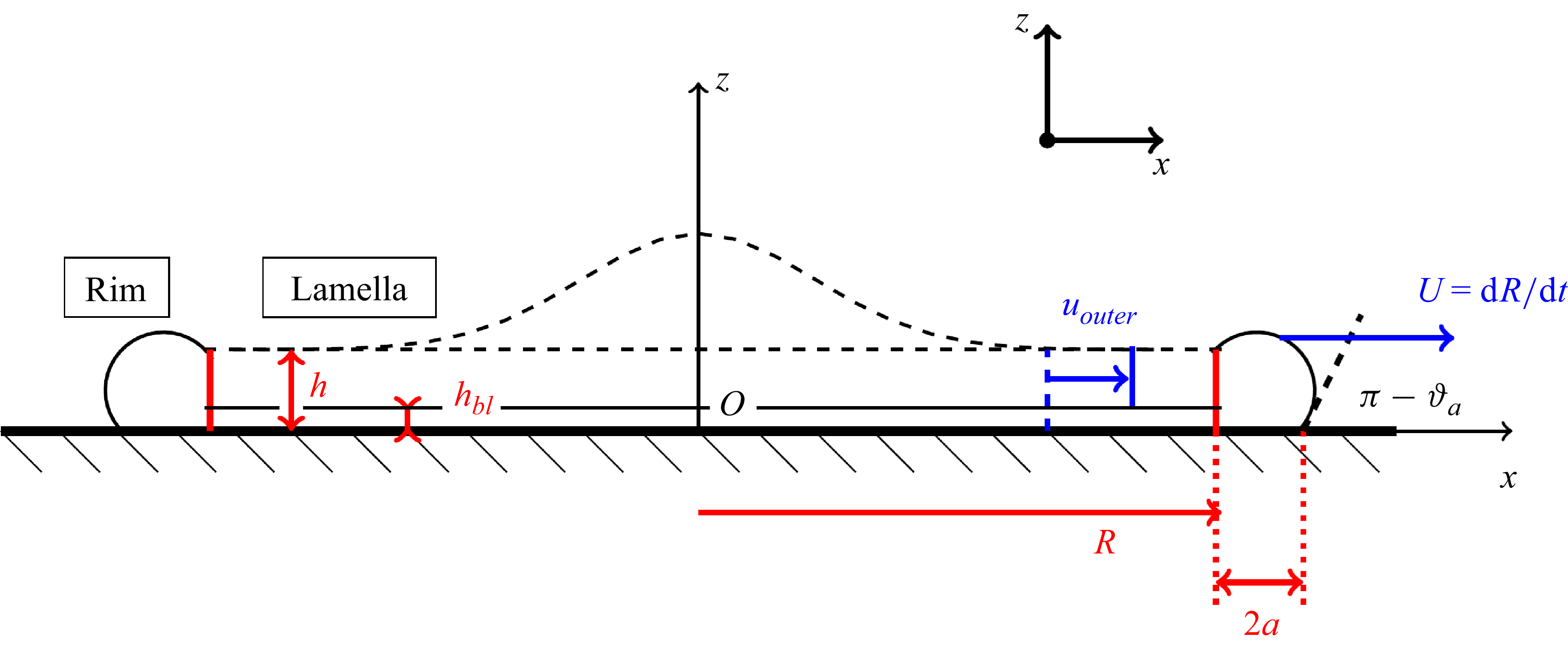


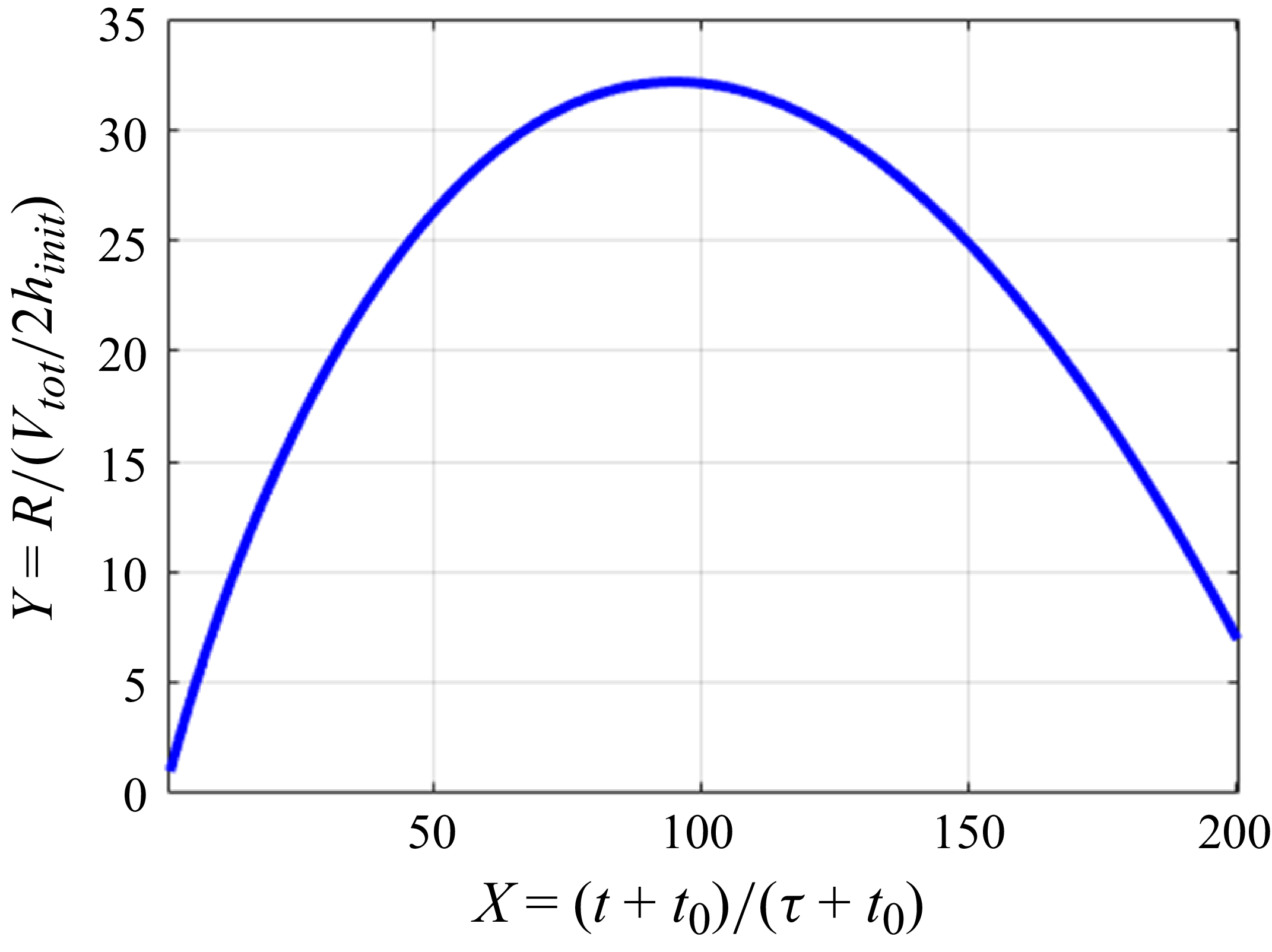

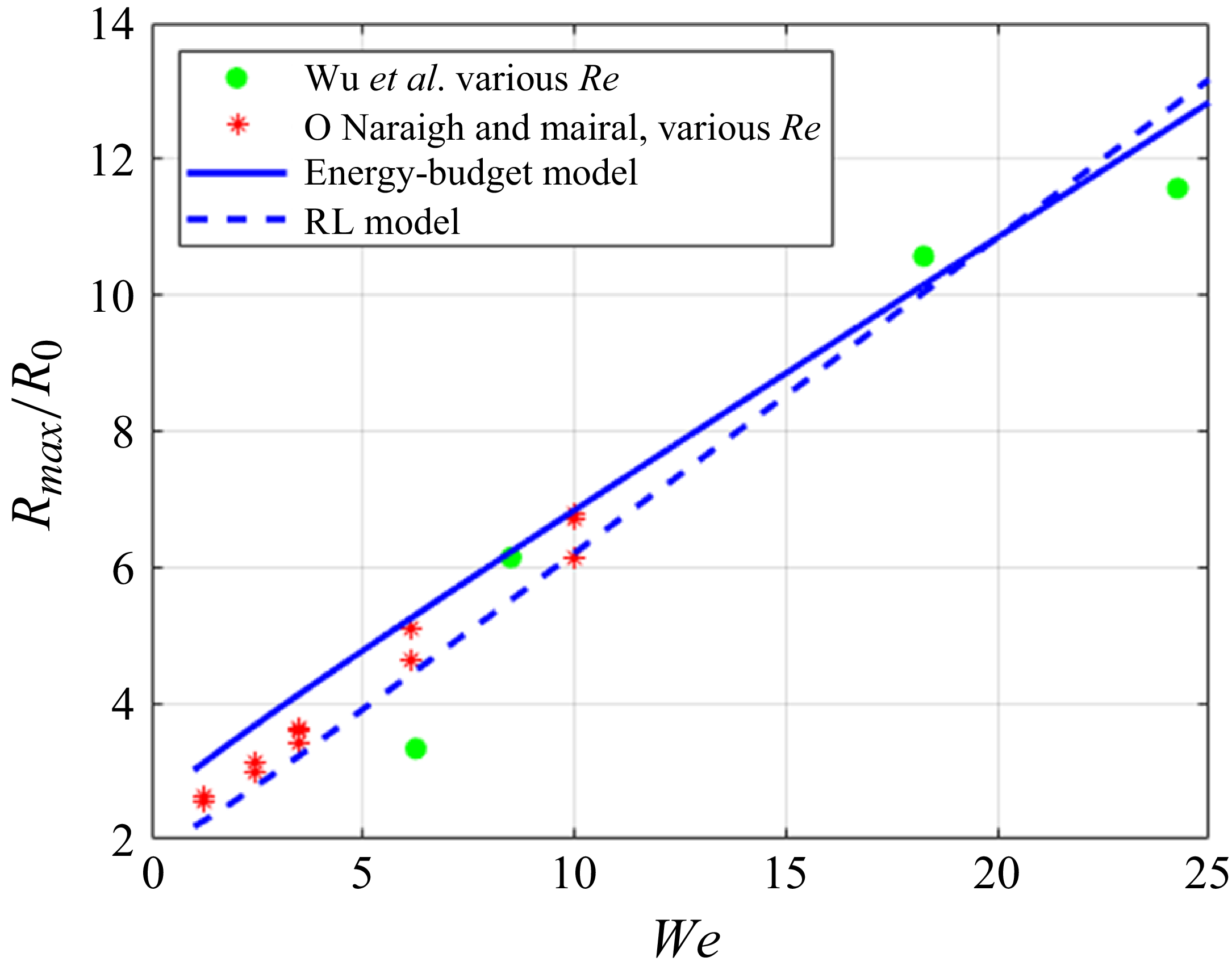


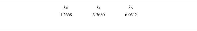


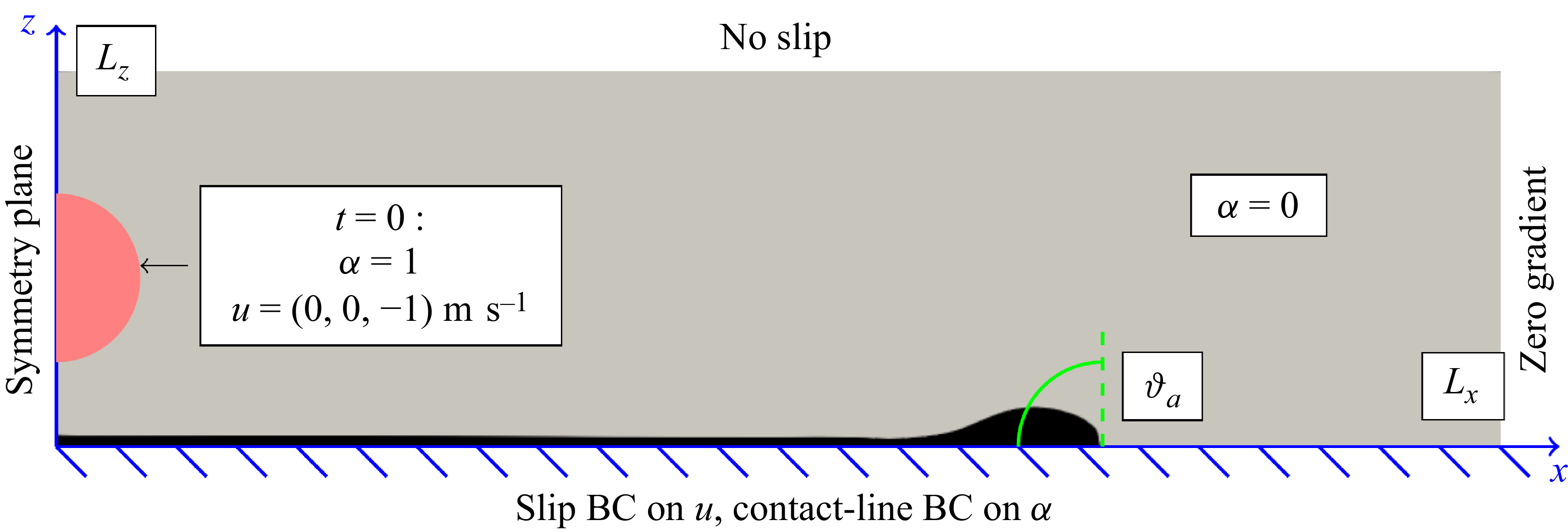


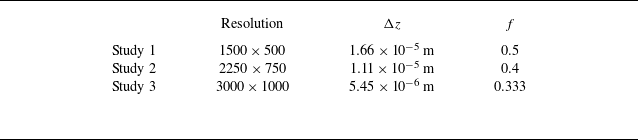

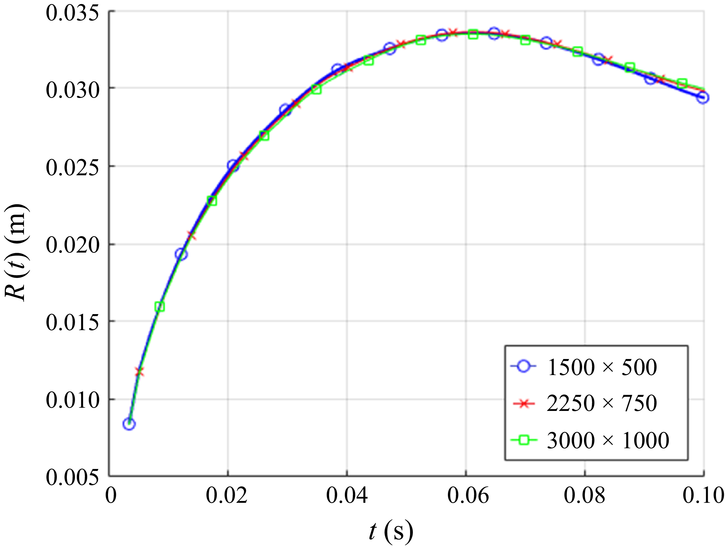


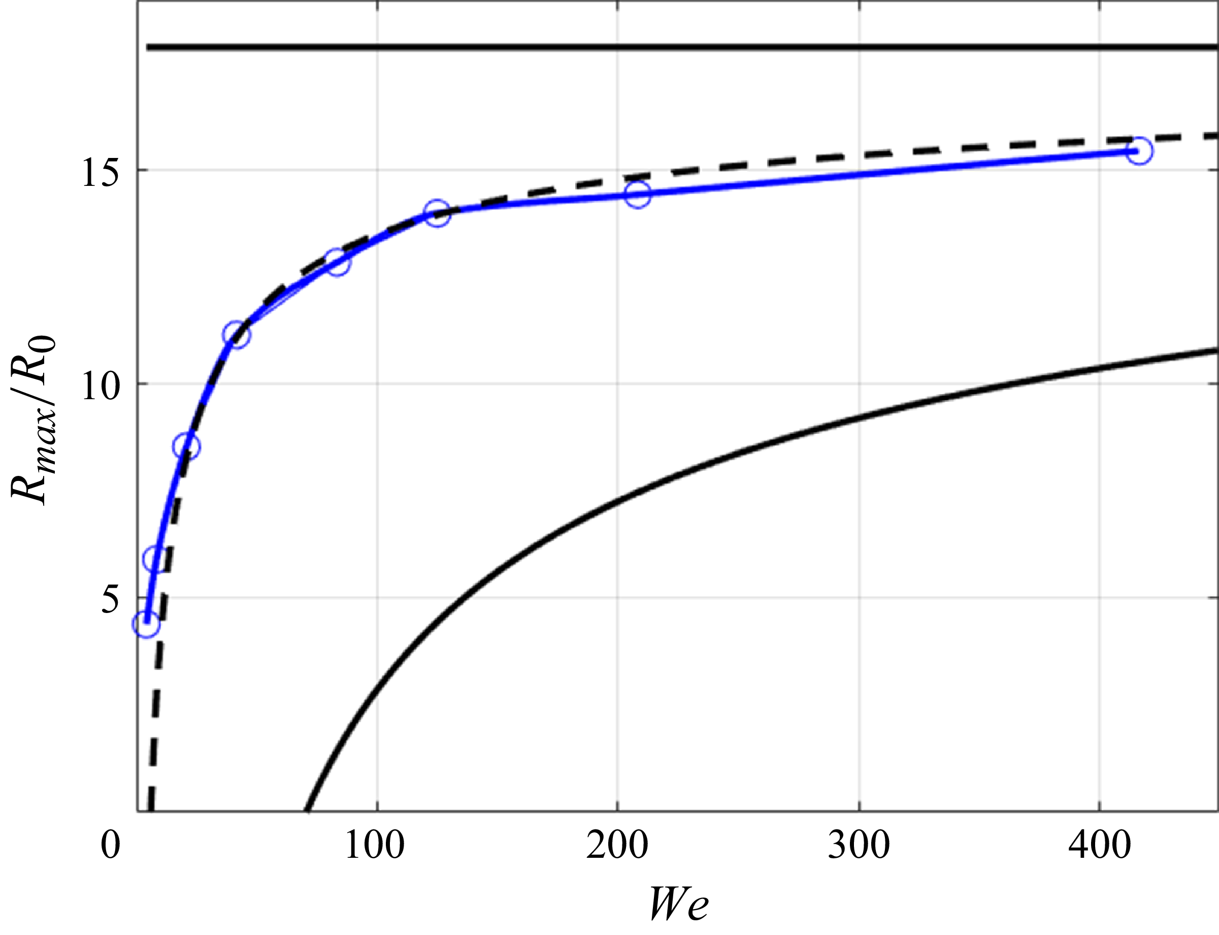


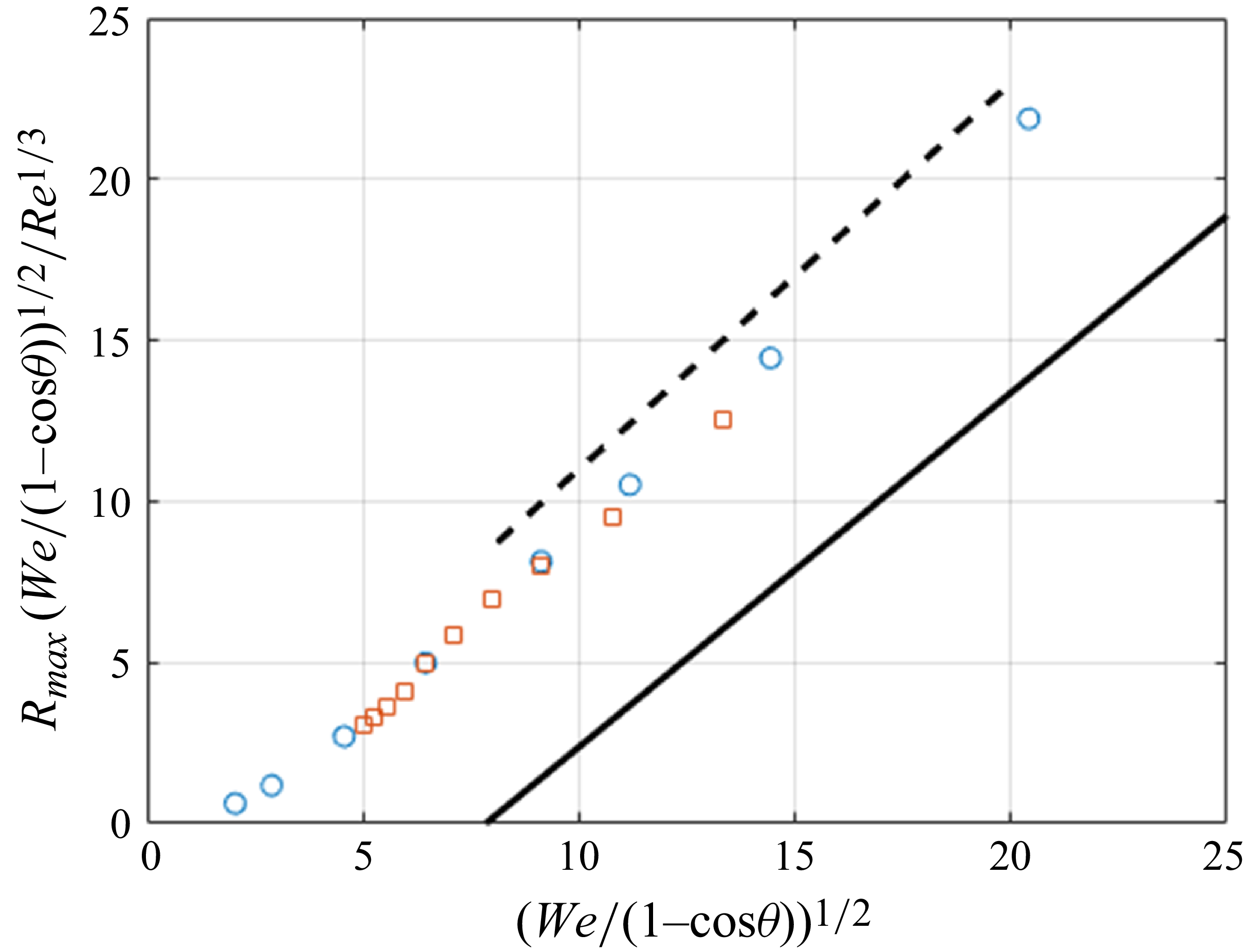


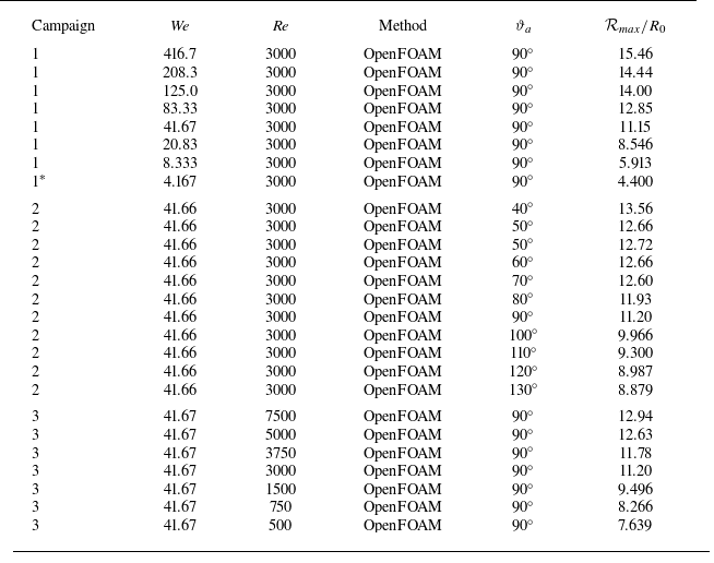

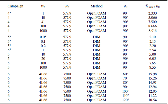


 Open access