





1. Introduction
Shock-wave/turbulent boundary layer interaction (STBLI) is a prevalent aerodynamic phenomenon in high-speed vehicles, arising in various applications such as supersonic inlets, over-expanded nozzles, control flaps and high-speed airfoils (Green Reference Green1970; Dolling Reference Dolling2001). The practical consequences of STBLI are often detrimental to vehicle performance. Strong interactions can induce boundary layer separation, resulting in significant pressure losses in supersonic inlets, which may, in severe cases, lead to engine unstart. Additionally, STBLI substantially increases the drag due to the transient separation bubble and generates intense localised thermal and mechanical loads, thereby accelerating material fatigue and compromising structural integrity (Tzong, Jacobs & Liguore Reference Tzong, Jacobs and Liguore2010; Gaitonde Reference Gaitonde2015).
Now, STBLI is known to exhibit a wide range of energetic frequency content. The high-frequency components originate primarily from the small-scale turbulence in the incoming boundary layer, and the mid-frequency range is linked to vortex shedding and the flapping motion of the separation bubble (Wu et al. Reference Wu, Meneveau and Mittal2020), while the low-frequency energy corresponds to the large-scale, unsteady behaviour of the separation bubble. These low-frequency unsteadiness phenomena have been consistently observed across a variety of canonical configurations, including compression ramps (Loginov, Adams & Zheltovodov Reference Loginov, Adams and Zheltovodov2006; Ganapathisubramani, Clemens & Dolling Reference Ganapathisubramani, Clemens and Dolling2009; Priebe et al. Reference Priebe, Tu, Rowley and Martín2016; Porter & Poggie Reference Porter and Poggie2019), impinging shocks (Dupont, Haddad & Debieve Reference Dupont, Haddad and Debieve2006; Pirozzoli & Grasso Reference Pirozzoli and Grasso2006; Pasquariello, Hickel & Adams Reference Pasquariello, Hickel and Adams2017; Laguarda et al. Reference Laguarda, Hickel, Schrijer and van Oudheusden2024), backward-facing steps (Hu et al. Reference Hu, Hickel, van and Bas2022), as well as swept (Huang & Estruch-Samper Reference Huang and Estruch-Samper2018; Ceci et al. Reference Ceci, Palumbo, Larsson and Pirozzoli2023) and impinging conical shocks (Zuo, Memmolo & Pirozzoli Reference Zuo, Memmolo and Pirozzoli2023). Understanding this low-frequency unsteadiness is of particular importance, as these motions may couple with structural modes and induce resonance, leading to potential structural failure in high-speed vehicles (Tzong et al. Reference Tzong, Jacobs and Liguore2010; Babinsky & Harvey Reference Babinsky and Harvey2011).
The low-frequency unsteady motions typically occur at frequencies one to two orders of magnitude lower than those of the turbulent boundary layer, especially around a Strouhal number of $St_{L_{sep}} = 0.01$
–
$St_{L_{sep}} = 0.01$
– $0.05$
(Clemens & Narayanaswamy Reference Clemens and Narayanaswamy2014; Weiss et al. Reference Weiss, Little, Threadgill and Gross2021; Gaitonde & Adler Reference Gaitonde and Adler2023), where
$0.05$
(Clemens & Narayanaswamy Reference Clemens and Narayanaswamy2014; Weiss et al. Reference Weiss, Little, Threadgill and Gross2021; Gaitonde & Adler Reference Gaitonde and Adler2023), where $L_{sep}$
is the separation length. Dussauge, Dupont & Debiève (Reference Dussauge, Dupont and Debiève2006) experimentally investigated STBLI over a wide range of Mach numbers and Reynolds numbers, including impinging interactions, compression ramps and three-dimensional fins, and reported that the low-frequency motion typically occurs at
$L_{sep}$
is the separation length. Dussauge, Dupont & Debiève (Reference Dussauge, Dupont and Debiève2006) experimentally investigated STBLI over a wide range of Mach numbers and Reynolds numbers, including impinging interactions, compression ramps and three-dimensional fins, and reported that the low-frequency motion typically occurs at $St_{L_{sep}} = 0.02$
–
$St_{L_{sep}} = 0.02$
– $0.05$
. Dupont et al. (Reference Dupont, Haddad and Debieve2006) reported that the characteristic low-frequency unsteadiness was
$0.05$
. Dupont et al. (Reference Dupont, Haddad and Debieve2006) reported that the characteristic low-frequency unsteadiness was $St_{L_{sep}} \approx 0.02 \pm 0.01$
in an impinging STBLI. Similar behaviour was also observed by Jenquin, Johnson & Narayanaswamy (Reference Jenquin, Johnson and Narayanaswamy2023) over an inward-turning axisymmetric compression ramp at
$St_{L_{sep}} \approx 0.02 \pm 0.01$
in an impinging STBLI. Similar behaviour was also observed by Jenquin, Johnson & Narayanaswamy (Reference Jenquin, Johnson and Narayanaswamy2023) over an inward-turning axisymmetric compression ramp at $St_{L_{sep}} \approx 0.019$
, and by Musta & Clemens (Reference Musta and Clemens2024) in a planar compression ramp, where the low-frequency motions were confined within
$St_{L_{sep}} \approx 0.019$
, and by Musta & Clemens (Reference Musta and Clemens2024) in a planar compression ramp, where the low-frequency motions were confined within $St_{L_{sep}} \lt 0.1$
. In addition to the experimental observations, such a low-frequency dynamics has been captured in high-fidelity numerical simulations. For instance, Pasquariello et al. (Reference Pasquariello, Hickel and Adams2017) identified dominant low-frequency modes around
$St_{L_{sep}} \lt 0.1$
. In addition to the experimental observations, such a low-frequency dynamics has been captured in high-fidelity numerical simulations. For instance, Pasquariello et al. (Reference Pasquariello, Hickel and Adams2017) identified dominant low-frequency modes around $St_{L_{sep}} \approx 0.03$
, while Touber & Sandham (Reference Touber and Sandham2009) and Agostini, Larchevêque & Dupont (Reference Agostini, Larchevêque and Dupont2015) observed a characteristic frequency around
$St_{L_{sep}} \approx 0.03$
, while Touber & Sandham (Reference Touber and Sandham2009) and Agostini, Larchevêque & Dupont (Reference Agostini, Larchevêque and Dupont2015) observed a characteristic frequency around $St_{L_{sep}} \approx 0.04$
in an impinging STBLI using large-eddy simulation (LES). Priebe & Martín (Reference Priebe and Martín2012), using direct numerical simulation (DNS) of STBLI over a compression ramp, observed that the characteristic low-frequency contents exist in the range of
$St_{L_{sep}} \approx 0.04$
in an impinging STBLI using large-eddy simulation (LES). Priebe & Martín (Reference Priebe and Martín2012), using direct numerical simulation (DNS) of STBLI over a compression ramp, observed that the characteristic low-frequency contents exist in the range of $0.01 \lt St_{L_{sep}} \lt 0.1$
. Likewise, Laguarda et al. (Reference Laguarda, Hickel, Schrijer and van Oudheusden2024) performed LES of impinging STBLI across a range of Reynolds numbers and reported the broadband low-frequency response in the same range. While the energy content of these low-frequency motions increases with Reynolds number, the Strouhal number range itself remains largely unaffected by the Reynolds number variations.
$0.01 \lt St_{L_{sep}} \lt 0.1$
. Likewise, Laguarda et al. (Reference Laguarda, Hickel, Schrijer and van Oudheusden2024) performed LES of impinging STBLI across a range of Reynolds numbers and reported the broadband low-frequency response in the same range. While the energy content of these low-frequency motions increases with Reynolds number, the Strouhal number range itself remains largely unaffected by the Reynolds number variations.
Despite extensive investigations, the origin of low-frequency unsteadiness in STBLI remains a subject of ongoing debate (Clemens & Narayanaswamy Reference Clemens and Narayanaswamy2014). The proposed mechanisms are broadly categorised into two categories: upstream and downstream sources. The upstream mechanism posits that low-frequency unsteadiness originates from large-scale structures in the incoming turbulent boundary layer. Early studies found that velocity and momentum fluctuations near the wall – including burst–sweep events and very-large-scale motions (VLSMs) – can modulate the separation shock motion through transient pressure and momentum exchanges (Beresh, Clemens & Dolling Reference Beresh, Clemens and Dolling2002; Ganapathisubramani et al. Reference Ganapathisubramani, Clemens and Dolling2006, Reference Ganapathisubramani, Clemens and Dolling2009). Although the observed correlation is typically modest and the influence diminishes with increasing separation extent (Souverein et al. Reference Souverein, Dupont, Debiève, Dussauge, van, Bas and Scarano2010; Clemens & Narayanaswamy Reference Clemens and Narayanaswamy2014), these findings support the view that upstream turbulence can influence the STBLI dynamics, particularly in incipient or intermittent separation regimes.
A central manifestation of downstream-induced unsteadiness is the so-called separation bubble breathing mode, characterised by large-scale expansion and contraction of the separation bubble coupled with unsteady shock motion. Several hypotheses have been proposed to explain the origin of this low-frequency behaviour of the separation bubble breathing. These include mechanisms emphasising the importance of shear-layer flapping (Piponniau et al. Reference Piponniau, Dussauge, DebiÈVe and Dupont2009; Huang & Estruch-Samper Reference Huang and Estruch-Samper2018), mass imbalance within the separation bubble (Jenquin et al. Reference Jenquin, Johnson and Narayanaswamy2023) and the influence of Görtler-like structures (Priebe et al. Reference Priebe, Tu, Rowley and Martín2016; Pasquariello et al. Reference Pasquariello, Hickel and Adams2017). In addition, global instability mechanisms have been suggested as intrinsic sources of unsteadiness. For example, Touber & Sandham (Reference Touber and Sandham2011) demonstrated that the separation bubble acts as a low-pass filter, selectively amplifying resonant global modes. More recently, Hao (Reference Hao2023) showed that the low-frequency shock motions can arise from the excitation of an intrinsic stationary global mode within the separation bubble by upstream disturbances.
The detached shear layer has been considered to be one of the prominent influential physics of the downstream mechanism. According to experimental (Dupont, Piponniau & Dussauge Reference Dupont, Piponniau and Dussauge2019) and numerical studies (Helm, Martín & Williams Reference Helm, Martín and Williams2021), the detached shear layer exhibits the key characteristics of a canonical compressible mixing layer, including self-similar mean profiles, linear spreading with convective Mach number dependence, large-scale Kelvin–Helmholtz (K–H) vortices and turbulence scaling laws consistent with the classical dimensional analysis. Piponniau et al. (Reference Piponniau, Dussauge, DebiÈVe and Dupont2009) proposed a mechanism based on the entrainment characteristics of the mixing layer at the edge of the separation, demonstrating that progressive mass loss from the recirculation zone induces bubble contraction, followed by rapid mass influx and bubble expansion. This cyclic process drives the large-scale, low-frequency shock motion. Building on this concept, Huang & Estruch-Samper (Reference Huang and Estruch-Samper2018) investigated the shear-layer behaviour using oil flow visualisation and surface pressure fluctuation measurements, emphasising that the periodic mass entrainment and ejection by the separated shear layer result in a cyclic depletion and replenishment of the bubble mass, which drives the breathing motion of the bubble and the associated low-frequency oscillations. In addition, Jenquin et al. (Reference Jenquin, Johnson and Narayanaswamy2023) utilised high-bandwidth dynamic pressure field measurements to show that the large-scale low-frequency motions of the separation shock are primarily driven by a mass imbalance within the separation bubble, and additionally identified that spanwise-offset pressure perturbations play a significant role in influencing the separation bubble dynamics. In contrast to these mass-based interpretations, Ben Hassan Saïdi et al. (Reference Ben Hassan Saïdi, Wang, Fournier, Tenaud and Robinet2025), who conducted a numerical study of transitional shock–boundary layer interaction with a laminar incoming boundary layer, proposed that the low-frequency breathing motion arises from nonlinear triadic interactions within the separation bubble, whereby energy is transferred from medium-frequency shear-layer modes to newly generated low-frequency modes through quadratic nonlinear coupling.
Another view attributes the unsteadiness to centrifugal (Görtler-type) instabilities. In boundary layers over concave walls, Görtler instability naturally generates streamwise-elongated, counter-rotating vortex pairs near the wall, forming characteristic mushroom-shaped velocity structures that bulge outward and then compress back toward the surface (Görtler Reference Görtler1954). In early investigations of STBLI, spanwise-alternating regions of low and high momentum were commonly observed using surface oil flow visualisation techniques (Settles, Fitzpatrick & Bogdonoff Reference Settles, Fitzpatrick and Bogdonoff1979; Schuelein & Trofimov Reference Schuelein and Trofimov2011) and time-averaged flow fields obtained from LES Loginov et al. (Reference Loginov, Adams and Zheltovodov2006), which have been interpreted as Görtler-like vortex or Görtler-like structure. The presence of Görtler instability was supported by the elevated Görtler numbers exceeding classical thresholds. In the separation region, the curvature of the streamlines induced by the separation bubble increases the Görtler number well beyond the critical criterion for centrifugal instability (Loginov et al. Reference Loginov, Adams and Zheltovodov2006; Priebe et al. Reference Priebe, Tu, Rowley and Martín2016; Pasquariello et al. Reference Pasquariello, Hickel and Adams2017). Additionally, Priebe et al. (Reference Priebe, Tu, Rowley and Martín2016) identified streamwise-elongated regions of low and high momentum originating at the shock foot and extending downstream, as revealed by low-frequency modes extracted through dynamic mode decomposition (DMD). Pasquariello et al. (Reference Pasquariello, Hickel and Adams2017) further provided evidence of counter-rotating streamwise vortices emerging near the bubble apex, based on a flow field from LES of an impinging STBLI. In addition, sparsity-promoting dynamic mode decomposition (SPDMD) of the two-dimensional skin-friction coefficient revealed streamwise streaks associated with the low-frequency mode, which drive the large-scale flapping motion of the reattachment line.
Despite these previous studies, doubts have been raised regarding the interpretation of the presence of Görtler vortices. Jenquin et al. (Reference Jenquin, Johnson and Narayanaswamy2023) proposed that the observed large-scale streaky structures result from shear-layer flapping rather than Görtler vortex-induced streaks due to the absence of distinct cellular patterns or mushroom-shaped features. Similarly, Baidya et al. (Reference Baidya, Scharnowski, Bross and Kähler2020), based on experimental observations, expressed uncertainty regarding the existence of Görtler vortices, despite observing the pronounced low-frequency pulsations of the separation bubble. They suggest that the observed structures may instead arise from the incursion of VLSMs into the interaction region. According to the recent fundamental study by Xu, Ricco & Marensi (Reference Xu, Ricco and Marensi2024), the nonlinear evolution of compressible Görtler vortices under varying levels of free-stream vortical disturbances (FVDs) revealed that the increased FVD intensity suppresses the formation of canonical mushroom-shaped vortices, even over concave walls, leading instead to streamwise-elongated streaks. Stemming from this finding, we infer that the centrifugal instability induced by the separation-related curvature fails to form the mushroom shapes in the presence of inflow turbulence in STBLI, and instead manifests as streaks.
Even though the modal analysis results from numerical simulations indicate the presence of large-scale counter-rotating streaky structures in the low-frequency content, their role as a coherent forcing mechanism for low-frequency unsteadiness remains unclear. A recent study by Laguarda et al. (Reference Laguarda, Hickel, Schrijer and van Oudheusden2024) identified counter-rotating vortex pairs across a wide range of Reynolds numbers in impinging STBLI using SPDMD of LES data. However, these structures were observed not only in the low-frequency range but also in the mid-frequency range, suggesting that the mere presence of Görtler-like vortices does not necessarily imply their involvement in driving the low-frequency dynamics.
In summary, despite the extensive efforts to elucidate the origin of low-frequency dynamics in STBLI, the underlying mechanism remains unclear. In particular, the connection between the shear-layer flapping and large-scale counter-rotating vortices is still ambiguous, and a unified explanation of their role in driving the low-frequency motion of the separation bubble is lacking.
To fill this gap, we performed numerical simulations of STBLI on compression ramps with varying degrees of corner rounding, which systematically modulate the extent of separation strength and detached shear layer, while maintaining sufficient streamline curvature to exceed the Görtler-number threshold, thereby satisfying a necessary condition for Görtler instability. As the ramp corner becomes increasingly rounded, the mean separation bubble weakens and eventually disappears for sufficiently large corner radii (Tong et al. Reference Tong, Li, Duan and Yu2017a ; Cao et al. Reference Cao, Hao, Guo, Wen and Klioutchnikov2023; Shi et al. Reference Shi, Liu, Ji, Sun, Liu, Li and Yu2025). Nevertheless, the geometric curvature maintains the streamline concavity, thereby preserving the potential for Görtler instability. By comparing sharp and rounded configurations, we aim to isolate and characterise the interaction between the detached shear layer and large-scale counter-rotating structures, and to assess its influence on the emergence of low-frequency unsteadiness.
To this end, DNSs are performed using a high-order in-house compressible flow solver to capture the complex dynamics of STBLI. The numerical methods and computational set-up are described in § 2. The simulation results and detailed analysis of the low-frequency dynamics are presented in § 3, and the main findings are summarised in § 4.
2. Methods
2.1. Numerical methods
In this study, an in-house code (Kang & Lee Reference Kang and Lee2024, Reference Kang and Lee2026) was employed to perform the DNSs. The governing equations are the three-dimensional, unsteady, compressible Navier–Stokes equations, expressed as follows:
 \begin{align} \frac {\partial \rho }{\partial t} + \frac {\partial }{\partial x_j} (\rho u_j) &= 0 , \end{align}
 \begin{align} \frac {\partial }{\partial t}(\rho u_i) + \frac {\partial }{\partial x_j}(\rho u_j u_i + p\delta _{\textit{ij}}-\tau _{\textit{ij}}) &= f_i , \end{align}
 \begin{align} \frac {\partial E}{\partial t} + \frac {\partial }{\partial x_j}(u_j E - S_{\textit{ij}} u_i + q_j) &= f_i u_i . \end{align}
The coordinate system is defined as $x_i = (x, y, z)$
, corresponding to the streamwise, wall-normal and spanwise directions, respectively. The origin of this coordinate system is located at the corner of the ramp. Here,
$x_i = (x, y, z)$
, corresponding to the streamwise, wall-normal and spanwise directions, respectively. The origin of this coordinate system is located at the corner of the ramp. Here, $\rho$
denotes the density,
$\rho$
denotes the density, $u_i=(u,v,w)$
is the velocity corresponding to
$u_i=(u,v,w)$
is the velocity corresponding to $x_i=(x,y,z)$
direction,
$x_i=(x,y,z)$
direction, $p$
is the pressure,
$p$
is the pressure, $\delta _{\textit{ij}}$
denotes the Kronecker delta,
$\delta _{\textit{ij}}$
denotes the Kronecker delta, $E = \rho (e + u_i u_i/2)$
presents the total fluid energy in which
$E = \rho (e + u_i u_i/2)$
presents the total fluid energy in which $e$
is the internal energy,
$e$
is the internal energy, $S_{\textit{ij}}$
presents the strain rate tensor,
$S_{\textit{ij}}$
presents the strain rate tensor, $q_i$
denotes the heat flux and
$q_i$
denotes the heat flux and $f_i$
is the body-force term that induces the flow transition. The viscous stress tensor,
$f_i$
is the body-force term that induces the flow transition. The viscous stress tensor, $\tau _{\textit{ij}}$
, is determined by the Newtonian fluid relationship
$\tau _{\textit{ij}}$
, is determined by the Newtonian fluid relationship
 \begin{eqnarray} \tau _{\textit{ij}} = \mu \left ( \frac {\partial u_i}{\partial x_j} + \frac {\partial u_j}{\partial x_i} \right ) - \frac {2}{3} \mu \delta _{\textit{ij}} \frac {\partial u_k}{\partial x_k}\ , \end{eqnarray}
where $\mu$
is the dynamic viscosity. The fluid is assumed to be a perfect gas with a heat capacity ratio of 1.4. The viscosity follows Sutherland’s law, while the thermal conductivity is computed using the Prandtl relation,
$\mu$
is the dynamic viscosity. The fluid is assumed to be a perfect gas with a heat capacity ratio of 1.4. The viscosity follows Sutherland’s law, while the thermal conductivity is computed using the Prandtl relation, $\kappa =\mu c_p /Pr$
, where the Prandtl number is
$\kappa =\mu c_p /Pr$
, where the Prandtl number is $Pr = 0.72$
and
$Pr = 0.72$
and $c_p$
is the heat capacity at constant pressure.
$c_p$
is the heat capacity at constant pressure.
The governing equations are solved in conservative form using the generalised coordinates $(\xi , \eta , \zeta )$
, which are transformed from the Cartesian coordinates
$(\xi , \eta , \zeta )$
, which are transformed from the Cartesian coordinates $(x, y, z)$
 \begin{eqnarray} \frac {\partial \bar {U}}{\partial t}+\frac {\partial \bar {E}}{\partial \xi }+\frac {\partial \bar {F}}{\partial \eta } + \frac {\partial \bar {G}}{\partial \zeta }={\bar {S}}_{\textit{ext}} , \end{eqnarray}
where $\bar {U}$
is the solution vector,
$\bar {U}$
is the solution vector, $\bar {S}_{{\textit{ext}}}$
is the external body-force vector and
$\bar {S}_{{\textit{ext}}}$
is the external body-force vector and $\bar {E}$
,
$\bar {E}$
, $\bar {F}$
and
$\bar {F}$
and $\bar {G}$
are the flux terms, including both convective and viscous contributions. These variables are defined as follows:
$\bar {G}$
are the flux terms, including both convective and viscous contributions. These variables are defined as follows:
 \begin{eqnarray} U &=& \begin{bmatrix} \rho \\ \rho u \\ \rho v \\ \rho w \\ \rho e \end{bmatrix}, \quad S_{\textit{ext}} = \begin{bmatrix} 0 \\ f_1 \\ f_2 \\ f_3 \\ f_1 u + f_2 v + f_3 w \end{bmatrix}, \nonumber \\ E &=& \begin{bmatrix} \rho u \\ \rho u^2 + p - \tau _{11} \\ \rho u v - \tau _{12} \\ \rho u w - \tau _{13} \\ (\rho e + p)u - (u \tau _{11} + v \tau _{12} + w \tau _{13}) + q_1 \end{bmatrix}. \end{eqnarray}
The bar denotes the converted vector in the generalised coordinate: $\bar {U}=U/J$
,
$\bar {U}=U/J$
, $\bar {S}_{\textit{ext}}=S_{\textit{ext}}/J$
and the converted flux terms are formulated following:
$\bar {S}_{\textit{ext}}=S_{\textit{ext}}/J$
and the converted flux terms are formulated following:
 \begin{eqnarray} \bar {E}=\frac {1}{J} \left (\frac {\partial \xi }{\partial x}E + \frac {\partial \xi }{\partial y}F + \frac {\partial \xi }{\partial z}G\right ) \! , \end{eqnarray}
where $J$
represents the Jacobian of the transformation
$J$
represents the Jacobian of the transformation $J=| \partial (x,y,z)/\partial (\xi ,\eta ,\zeta )|$
. The spatial derivatives are computed using a compact finite-difference scheme (Lele Reference Lele1992) that provides spectral-like resolution, achieving sixth-order accuracy both at the interior domain and near the boundaries. The time integration is performed using a third-order explicit Runge–Kutta method. Numerical stability is maintained through eight-order Pade-type non-dispersive spatial filters (Gaitonde Reference Gaitonde2015), applied to the solution vector at the final Runge–Kutta step. To mitigate the numerical oscillations caused by turbulent structures with steep gradients, the localised artificial diffusivity method, developed by Kawai & Lele (Reference Kawai and Lele2008), is employed. This approach adjusts viscosity and thermal conductivity, effectively suppressing spurious oscillations while preserving the accuracy of the solution.
$J=| \partial (x,y,z)/\partial (\xi ,\eta ,\zeta )|$
. The spatial derivatives are computed using a compact finite-difference scheme (Lele Reference Lele1992) that provides spectral-like resolution, achieving sixth-order accuracy both at the interior domain and near the boundaries. The time integration is performed using a third-order explicit Runge–Kutta method. Numerical stability is maintained through eight-order Pade-type non-dispersive spatial filters (Gaitonde Reference Gaitonde2015), applied to the solution vector at the final Runge–Kutta step. To mitigate the numerical oscillations caused by turbulent structures with steep gradients, the localised artificial diffusivity method, developed by Kawai & Lele (Reference Kawai and Lele2008), is employed. This approach adjusts viscosity and thermal conductivity, effectively suppressing spurious oscillations while preserving the accuracy of the solution.
The transition to turbulent flow is achieved using the counter-flow body-force tripping method by Poggie & Smits (Reference Poggie and Smits2001). The body force $f_i$
is given as
$f_i$
is given as
 \begin{equation} f = \frac {2D_c}{\pi l_1 l_2 l_3} \sin ^2\left (\pi \frac {z-X_3}{l_3}\right ) \exp \left [-\left (\frac {x-X_1}{l_1}\right )^2 - \left (\frac {y-X_2}{l_2}\right )^2\right ]\!. \end{equation}
The force distribution exhibits a Gaussian profile in the streamwise and wall-normal direction, while in the spanwise direction, it follows the square of the sine function. Here, ( $X_1$
,
$X_1$
, $X_2$
,
$X_2$
, $X_3$
) denote the centre coordinates of the forcing region, and
$X_3$
) denote the centre coordinates of the forcing region, and $(l_1,l_2,l_3)$
represent the spatial extent of the forcing region, both of which are user-defined parameters. The parameter
$(l_1,l_2,l_3)$
represent the spatial extent of the forcing region, both of which are user-defined parameters. The parameter $D_c$
controls the magnitude of the body force. Larger values of
$D_c$
controls the magnitude of the body force. Larger values of $D_c$
can lead to numerical instability, while smaller values necessitate a longer tripping region to achieve turbulence. Detailed discussions on parameter selection are provided in a previous study by Kang & Lee (Reference Kang and Lee2024). The body force is decomposed as
$D_c$
can lead to numerical instability, while smaller values necessitate a longer tripping region to achieve turbulence. Detailed discussions on parameter selection are provided in a previous study by Kang & Lee (Reference Kang and Lee2024). The body force is decomposed as $f_i=(f\cos 179^\circ , f\sin 179^\circ ,0)$
, ensuring that the force direction is nearly parallel to the wall.
$f_i=(f\cos 179^\circ , f\sin 179^\circ ,0)$
, ensuring that the force direction is nearly parallel to the wall.
2.2. Simulation set-up
The flow conditions adopted in the present study are based on the experimental configuration reported by Bookey, Wyckham & Smits (Reference Bookey, Wyckham and Smits2005), which investigated STBLI over a $24^\circ$
compression ramp. This dataset has been extensively used in previous numerical studies (Wu & Martin Reference Wu and Martin2008; Priebe & Martín Reference Priebe and Martín2012; Tong et al. Reference Tong, Li, Duan and Yu2017a
; Kokkinakis et al. Reference Kokkinakis, Drikakis, Ritos and Spottswood2020; Guo et al. Reference Guo, Fang, Zhang and Li2022; Shi & Yan Reference Shi and Yan2023). The inflow conditions are summarised in table 1, where the
$24^\circ$
compression ramp. This dataset has been extensively used in previous numerical studies (Wu & Martin Reference Wu and Martin2008; Priebe & Martín Reference Priebe and Martín2012; Tong et al. Reference Tong, Li, Duan and Yu2017a
; Kokkinakis et al. Reference Kokkinakis, Drikakis, Ritos and Spottswood2020; Guo et al. Reference Guo, Fang, Zhang and Li2022; Shi & Yan Reference Shi and Yan2023). The inflow conditions are summarised in table 1, where the $\infty$
and
$\infty$
and $w$
subscripts are inflow and wall properties, respectively. Here,
$w$
subscripts are inflow and wall properties, respectively. Here, $M$
is the Mach number,
$M$
is the Mach number, $T$
denotes temperature and
$T$
denotes temperature and ${\textit{Re}}$
indicates the Reynolds number.
${\textit{Re}}$
indicates the Reynolds number.
Flow conditions.

(a) Configuration of the computational domain and (b) schematic of a curved compression ramp.

Grid configuration of (a) R24 (b) C7 and (c) C14 near the ramp corner. The figure is plotted on every 10th and 5th grid line in the x and y directions.

The geometry of the computational domain is shown in figure 1(a). The flat plate has dimensions of $L_x \times L_z = 237.5 \times 35$
mm
$L_x \times L_z = 237.5 \times 35$
mm $^2$
(
$^2$
( $\approx 35.4\delta _0 \times 5.2\delta _0$
), and a ramp of length 54.5 mm (
$\approx 35.4\delta _0 \times 5.2\delta _0$
), and a ramp of length 54.5 mm ( $\approx 8.1\delta _0$
) with the same width, where
$\approx 8.1\delta _0$
) with the same width, where $\delta _0$
is the incoming boundary layer thickness. While the ramp corners are fixed, the curved corner is determined by the deflection angle
$\delta _0$
is the incoming boundary layer thickness. While the ramp corners are fixed, the curved corner is determined by the deflection angle $\theta$
and the radius of the curvature
$\theta$
and the radius of the curvature $R$
, as depicted in figure 1(b). Three ramp configurations are studied in the present study. The first configuration, labelled as ’R24’, is a 24
$R$
, as depicted in figure 1(b). Three ramp configurations are studied in the present study. The first configuration, labelled as ’R24’, is a 24 $^\circ$
compression ramp, while the others, ’C7’ and ’C14’, are curved compression ramps with radii of curvature approximately 7 and 14 times
$^\circ$
compression ramp, while the others, ’C7’ and ’C14’, are curved compression ramps with radii of curvature approximately 7 and 14 times $\delta _0$
, respectively, where 0 subscripts refer to the reference station located 36 mm (
$\delta _0$
, respectively, where 0 subscripts refer to the reference station located 36 mm ( $-5.31 \delta _0$
) upstream of the ramp corner.
$-5.31 \delta _0$
) upstream of the ramp corner.
The computational domain consists of a structured grid of $N_x \times N_y \times N_z =2865 \times 298 \times 420$
grid points in the
$N_x \times N_y \times N_z =2865 \times 298 \times 420$
grid points in the $x$
,
$x$
, $y$
and
$y$
and $z$
directions, respectively, totalling approximately 358 million points. Side views (
$z$
directions, respectively, totalling approximately 358 million points. Side views ( $x{-}y$
plane) of the grid for each ramp configuration are illustrated in figure 2. All three cases have the same grid resolution. The grid points in the
$x{-}y$
plane) of the grid for each ramp configuration are illustrated in figure 2. All three cases have the same grid resolution. The grid points in the $x$
direction are uniformly spaced, and power-law-based sponge layers are attached at the exit. In the
$x$
direction are uniformly spaced, and power-law-based sponge layers are attached at the exit. In the $y$
direction, the grids are clustered near the wall using a hyperbolic tangent function up to a height of
$y$
direction, the grids are clustered near the wall using a hyperbolic tangent function up to a height of $15$
mm (2.24
$15$
mm (2.24 $\delta _0$
), followed by a power-law-based sponge layer above. The
$\delta _0$
), followed by a power-law-based sponge layer above. The $z$
direction features uniform spacing. The grid resolution in the
$z$
direction features uniform spacing. The grid resolution in the $x$
and
$x$
and $z$
directions is
$z$
directions is $\Delta x^+=4.6$
and
$\Delta x^+=4.6$
and $\Delta z^+=4.2$
, respectively, based on the wall unit calculated at the reference station. At the wall, the grid spacing in the
$\Delta z^+=4.2$
, respectively, based on the wall unit calculated at the reference station. At the wall, the grid spacing in the $y$
direction is
$y$
direction is $\Delta y_w^+=0.42$
. The choices for the size of the computational domain and grid resolutions are summarised in table 2, along with a comparison with other DNS studies conducted under the same flow configuration (Priebe & Martín Reference Priebe and Martín2012; Tong et al. Reference Tong, Yu, Tang and Li2017b
; Kokkinakis et al. Reference Kokkinakis, Drikakis, Ritos and Spottswood2020; Guo et al. Reference Guo, Fang, Zhang and Li2022). It is important to note that the grid resolutions in table 2 are evaluated in the upstream turbulent boundary layer. As the flow evolves downstream through the STBLI, the viscous length scale decreases due to the flow compression and increased wall shear, thereby increasing the resolution requirements. The current grid spacing satisfies the DNS resolution criteria (Ceci, Palumbo & Pirozzoli Reference Ceci, Palumbo and Pirozzoli2026) from the incoming turbulent boundary layer to approximately the reattachment point, capturing the essential STBLI flow physics.
$\Delta y_w^+=0.42$
. The choices for the size of the computational domain and grid resolutions are summarised in table 2, along with a comparison with other DNS studies conducted under the same flow configuration (Priebe & Martín Reference Priebe and Martín2012; Tong et al. Reference Tong, Yu, Tang and Li2017b
; Kokkinakis et al. Reference Kokkinakis, Drikakis, Ritos and Spottswood2020; Guo et al. Reference Guo, Fang, Zhang and Li2022). It is important to note that the grid resolutions in table 2 are evaluated in the upstream turbulent boundary layer. As the flow evolves downstream through the STBLI, the viscous length scale decreases due to the flow compression and increased wall shear, thereby increasing the resolution requirements. The current grid spacing satisfies the DNS resolution criteria (Ceci, Palumbo & Pirozzoli Reference Ceci, Palumbo and Pirozzoli2026) from the incoming turbulent boundary layer to approximately the reattachment point, capturing the essential STBLI flow physics.
The grid information of the present and reference simulations.

The spanwise domain length is wider than the previous DNS studies with the same configuration listed in table 2, to accurately capture the spanwise-alternating counter-rotating large-scale structures. According to recent studies, Zhang et al. (Reference Zhang, Hao and Uy2025a
) performed LES of STBLI over a $25^\circ$
compression ramp at Mach 2.95, while Soldati et al. (Reference Soldati, Ceci, Palumbo and Pirozzoli2026) investigated STBLI over a
$25^\circ$
compression ramp at Mach 2.95, while Soldati et al. (Reference Soldati, Ceci, Palumbo and Pirozzoli2026) investigated STBLI over a $24^\circ$
ramp at Mach 2.9 and
$24^\circ$
ramp at Mach 2.9 and ${\textit{Re}}_\theta \approx 1200$
. Both studies reported that the large-scale spanwise motions exhibit characteristic wavelengths of approximately 2
${\textit{Re}}_\theta \approx 1200$
. Both studies reported that the large-scale spanwise motions exhibit characteristic wavelengths of approximately 2 $L_{sep}$
. Accordingly, capturing the reported large-scale spanwise motions requires wider spanwise domain length which may affect the current observations on the counter-rotating structures.
$L_{sep}$
. Accordingly, capturing the reported large-scale spanwise motions requires wider spanwise domain length which may affect the current observations on the counter-rotating structures.
The initial condition in the simulation is set to match the prescribed flow conditions from the experiment of Bookey et al. (Reference Bookey, Wyckham and Smits2005), as listed in table 1. The inflow boundary layer is modelled using a laminar Blasius profile and the tripping method is applied 6.25 mm (0.93 $\delta _0$
) downstream of the inlet. The wall is treated with a no-slip isothermal boundary condition, where
$\delta _0$
) downstream of the inlet. The wall is treated with a no-slip isothermal boundary condition, where $T_w/T_\infty =2.87$
. For the streamwise and wall-normal outflow boundaries, the values are extrapolated from the interior of the computational domain. In the spanwise direction, periodic boundary conditions are imposed. The averaging time window used in the simulation is
$T_w/T_\infty =2.87$
. For the streamwise and wall-normal outflow boundaries, the values are extrapolated from the interior of the computational domain. In the spanwise direction, periodic boundary conditions are imposed. The averaging time window used in the simulation is $1200 u_\infty /\delta _0$
, which is significantly longer than the previous DNS studies that conducted
$1200 u_\infty /\delta _0$
, which is significantly longer than the previous DNS studies that conducted $200-400 u_\infty /\delta _0$
of simulation time (Wu & Martin Reference Wu and Martin2007; Priebe & Martín Reference Priebe and Martín2012; Kokkinakis et al. Reference Kokkinakis, Drikakis, Ritos and Spottswood2020; Shi & Yan Reference Shi and Yan2023; Kang & Lee Reference Kang and Lee2024).
$200-400 u_\infty /\delta _0$
of simulation time (Wu & Martin Reference Wu and Martin2007; Priebe & Martín Reference Priebe and Martín2012; Kokkinakis et al. Reference Kokkinakis, Drikakis, Ritos and Spottswood2020; Shi & Yan Reference Shi and Yan2023; Kang & Lee Reference Kang and Lee2024).
3. Results
3.1. Incoming turbulent boundary layer
The incoming turbulent boundary layer (TBL) is generated using the turbulent tripping method. The boundary layer statistics are evaluated at the reference location $x_0$
, which is positioned 5.37
$x_0$
, which is positioned 5.37 $\delta _0$
upstream of the ramp corner, matching the streamwise distance used in the experiment by Bookey et al. (Reference Bookey, Wyckham and Smits2005). Table 3 compares
$\delta _0$
upstream of the ramp corner, matching the streamwise distance used in the experiment by Bookey et al. (Reference Bookey, Wyckham and Smits2005). Table 3 compares $\delta _0$
, momentum thickness
$\delta _0$
, momentum thickness $\theta _0$
, Reynolds number based on momentum thickness
$\theta _0$
, Reynolds number based on momentum thickness ${\textit{Re}}_\theta = \rho _\infty u_\infty \theta _0 / \mu _\infty$
and skin-friction coefficient
${\textit{Re}}_\theta = \rho _\infty u_\infty \theta _0 / \mu _\infty$
and skin-friction coefficient $C_f$
. The present DNS matches the experimental values with high accuracy.
$C_f$
. The present DNS matches the experimental values with high accuracy.
Flow parameters at the reference station.

In this study, two types of averagings are conducted for the variable $\phi$
: Reynolds time averaging denoted by
$\phi$
: Reynolds time averaging denoted by $\overline {\phi }$
and Favre time averaging denoted by
$\overline {\phi }$
and Favre time averaging denoted by $\langle {\phi }\rangle =\overline {\rho \phi }/\overline {\rho }$
. The fluctuation components are defined as follows:
$\langle {\phi }\rangle =\overline {\rho \phi }/\overline {\rho }$
. The fluctuation components are defined as follows: $\phi \prime=\phi -\overline {\phi }$
represents the Reynolds fluctuation, and
$\phi \prime=\phi -\overline {\phi }$
represents the Reynolds fluctuation, and $\phi \prime\prime=\phi -\langle {\phi }\rangle$
represents the Favre fluctuation.
$\phi \prime\prime=\phi -\langle {\phi }\rangle$
represents the Favre fluctuation.
Figure 3(a) shows the mean streamwise velocity profile, compared with previous DNS (Wu & Martin Reference Wu and Martin2008; Soldati, Ceci & Pirozzoli Reference Soldati, Ceci and Pirozzoli2024) and experimental data (Bookey et al. Reference Bookey, Wyckham and Smits2005). Excellent agreement is observed, particularly with the experimental dataset. Figure 3(b) presents the van Driest transformed velocity profile, defined as
 \begin{eqnarray} \langle {u}\rangle _{VD} = \int _{0}^{\langle {u}\rangle } \left (\frac {\overline {\rho }}{\overline {\rho }_w}\right )^{\tfrac {1}{2}} d\langle {u}\rangle , \end{eqnarray}
where $u^+ = u/u_\tau$
, and the friction velocity is
$u^+ = u/u_\tau$
, and the friction velocity is $u_\tau = \sqrt {\tau _w / \rho _w}$
. The van Driest transformed velocity profile yields a collapse in the inner region, displaying the expected linear viscous sublayer and logarithmic overlap region, consistent with that of canonical TBLs (Wu & Martin Reference Wu and Martin2008).
$u_\tau = \sqrt {\tau _w / \rho _w}$
. The van Driest transformed velocity profile yields a collapse in the inner region, displaying the expected linear viscous sublayer and logarithmic overlap region, consistent with that of canonical TBLs (Wu & Martin Reference Wu and Martin2008).
(a) Mean streamwise velocity profile and (b) van Driest transformed mean streamwise velocity profile at $x_0$
.
$x_0$
.

Figures 4(a) and 4(b) show the density-scaled normal Reynolds stresses plotted in the inner and outer coordinates, respectively. The present DNS captures the correct peak values and the overall distribution, in good agreement with reference data from Pirozzoli, Bernardini & Grasso (Reference Pirozzoli, Bernardini and Grasso2010) and Tong et al. (Reference Tong, Li, Duan and Yu2017a ). Figure 4(c) displays the wall-normal distribution of pressure fluctuation intensity, expressed in root-mean-square (r.m.s.) of the wall pressure, which compares well with the previous DNS results of Bernardini, Pirozzoli & Grasso (Reference Bernardini, Pirozzoli and Grasso2011) and Cai et al. (Reference Cai, Yu, Sun, Ye, Liu and Yuan2022).
Profile of density-scaled turbulent intensity in (a) inner and (b) outer scale, and (c) r.m.s. of wall pressure fluctuation at $x_0$
.
$x_0$
.

Instantaneous streamwise velocity contour at plane of $x/\delta _0\approx 4$
,
$x/\delta _0\approx 4$
, $y^*/\delta _0\approx 0.05$
and
$y^*/\delta _0\approx 0.05$
and $z/\delta _0\approx 0$
for (a) R24, (b) C7 and (c) C14.
$z/\delta _0\approx 0$
for (a) R24, (b) C7 and (c) C14.

3.2. Instantaneous and mean flow field
Figure 5 presents the instantaneous streamwise velocity for R24, C7 and C14. The streamwise velocity is contoured at the planes $x/\delta _0\approx 4$
,
$x/\delta _0\approx 4$
, $y^*/\delta _0\approx 0.05$
and
$y^*/\delta _0\approx 0.05$
and $z/\delta _0\approx 0$
, where
$z/\delta _0\approx 0$
, where $y^*$
denotes the wall-normal distance. Compared with R24, the separation region, indicated in red, is reduced in C7, while in C14, no pronounced separation is observed. As the high- and low-speed near-wall streaks of the TBL pass through the separation, they undergo breakdown. In R24 and C7, the separation bubble exhibits a streaky structure that becomes more pronounced on a larger scale in the reattachment region than in the separation region. This is consistent with previous studies that the reattachment line exhibits large-scale streaky patterns, as demonstrated with contours of the skin-friction coefficient (Pasquariello et al. Reference Pasquariello, Hickel and Adams2017; Laguarda et al. Reference Laguarda, Hickel, Schrijer and van Oudheusden2024; Zhang et al. Reference Zhang, Guo, Dang and Li2024). At the downstream of the ramp corner, the large-scale high- and low-speed streaky structures are observed. These structures intermittently emerge, a characteristic that is also observed in experimental observations using an ice-cluster-based planar laser scattering technique over an impinging STBLI by Zhuang et al. (Reference Zhuang, Tan, Li, Sheng and Zhang2018). In C14, the large-scale streaks grow downstream of the ramp corner, but the size remain relatively small compared with those in R24 and C7.
$y^*$
denotes the wall-normal distance. Compared with R24, the separation region, indicated in red, is reduced in C7, while in C14, no pronounced separation is observed. As the high- and low-speed near-wall streaks of the TBL pass through the separation, they undergo breakdown. In R24 and C7, the separation bubble exhibits a streaky structure that becomes more pronounced on a larger scale in the reattachment region than in the separation region. This is consistent with previous studies that the reattachment line exhibits large-scale streaky patterns, as demonstrated with contours of the skin-friction coefficient (Pasquariello et al. Reference Pasquariello, Hickel and Adams2017; Laguarda et al. Reference Laguarda, Hickel, Schrijer and van Oudheusden2024; Zhang et al. Reference Zhang, Guo, Dang and Li2024). At the downstream of the ramp corner, the large-scale high- and low-speed streaky structures are observed. These structures intermittently emerge, a characteristic that is also observed in experimental observations using an ice-cluster-based planar laser scattering technique over an impinging STBLI by Zhuang et al. (Reference Zhuang, Tan, Li, Sheng and Zhang2018). In C14, the large-scale streaks grow downstream of the ramp corner, but the size remain relatively small compared with those in R24 and C7.
(a–c) Instantaneous numerical schlieren and (d–f) normalised mean density gradient for R24, C7 and C14, respectively. Major flow features are indicated in (d): (1) shear layer, (2) detached shear layer, (3) separation shock and (4) secondary shock.

Instantaneous visualisations of the numerical schlieren in the x–y plane are presented in figure 6(a–c). The numerical schlieren is defined as
 \begin{eqnarray} Sch=0.8\exp \left [\frac {-10(|\boldsymbol{\nabla }\rho |-|\boldsymbol{\nabla }\rho |_{\textit{min}})}{(|\boldsymbol{\nabla }\rho |_{\textit{max}}-|\boldsymbol{\nabla }\rho |_{\textit{min}})}\right ]. \end{eqnarray}
The straight separation shocks in R24 and C7 are clearly visible, and penetrate into the boundary layer. Downstream of the ramp corner, clusters of travelling shocklets are observed. For the highly rounded case, C14, the shock does not manifest as a distinct straight shock wave. Instead, it gradually transitions into a fan of compressive waves, which is consistent with the findings of Tong et al. (Reference Tong, Li, Duan and Yu2017a ). Additionally, in C14, large-scale turbulent outer structures remain attached to the wall, whereas in R24 and C7, these structures undergo roll-up.
To further investigate the turbulent and shock structures, the mean density gradient is illustrated in figure 6(d–f). The figure highlights the major features of the STBLI: (1) shear layer, (2) detached shear layer, (3) separation shock and (4) secondary shock. For R24, both the separation shock and secondary shock are distinctly visible, forming a well-defined $\lambda$
-structure. In contrast, for C7, the secondary shock is less prominent, leading to the collapse of the
$\lambda$
-structure. In contrast, for C7, the secondary shock is less prominent, leading to the collapse of the $\lambda$
-structure and the secondary shock is distributed over a broader area. In the case of C14, the shock does not penetrate deeply into the boundary layer. Instead, it transitions into a compression fan, consistent with observations from the instantaneous schlieren. This fan structure extends downstream of the ramp corner, with its intensity gradually decreasing.
$\lambda$
-structure and the secondary shock is distributed over a broader area. In the case of C14, the shock does not penetrate deeply into the boundary layer. Instead, it transitions into a compression fan, consistent with observations from the instantaneous schlieren. This fan structure extends downstream of the ramp corner, with its intensity gradually decreasing.
Another primary feature observed in the mean density gradient is the detached shear layer. Due to the relaminarisation characteristics of the flow reversal within the separation bubble, the shear layer detaches from the wall. Compared with R24, the height of the detached shear layer around the ramp corner is lower in C7. In contrast, the distinct detached shear layer is not observed in C14, yet the intensified shear layer is formed downstream of the ramp corner.
3.3. Flow separation and its unsteadiness
Figure 7(a) presents the streamwise distribution of the time- and spanwise-averaged skin-friction coefficient, $C_f$
. At the reference station, the computed
$C_f$
. At the reference station, the computed $C_f$
shows excellent agreement with the experimental data of Bookey et al. (Reference Bookey, Wyckham and Smits2005), with both the separation point (
$C_f$
shows excellent agreement with the experimental data of Bookey et al. (Reference Bookey, Wyckham and Smits2005), with both the separation point ( $x_s$
) and the reattachment point (
$x_s$
) and the reattachment point ( $x_r$
) for the R24 case closely matching the experimental values. The separation length, defined as
$x_r$
) for the R24 case closely matching the experimental values. The separation length, defined as $L_s = x_r - x_s$
, estimated from the simulation, agrees well with the experimental measurement. In addition, the overall shape of the
$L_s = x_r - x_s$
, estimated from the simulation, agrees well with the experimental measurement. In addition, the overall shape of the $C_f$
curve exhibits good agreement with other DNS results by Guo et al. (Reference Guo, Fang, Zhang and Li2022). For C14,
$C_f$
curve exhibits good agreement with other DNS results by Guo et al. (Reference Guo, Fang, Zhang and Li2022). For C14, $C_f$
is compared with the DNS results of Tong et al. (Reference Tong, Li, Duan and Yu2017a
) under the same configuration. The comparison shows consistent trends with the DNS data. The remaining differences in the absolute value of
$C_f$
is compared with the DNS results of Tong et al. (Reference Tong, Li, Duan and Yu2017a
) under the same configuration. The comparison shows consistent trends with the DNS data. The remaining differences in the absolute value of $C_f$
are attributed to discrepancies in the upstream conditions.
$C_f$
are attributed to discrepancies in the upstream conditions.
(a) Streamwise distribution of skin-friction coefficient and (b) statistical probability of flow reversal.

For R24 and C7, a mean separation region characterised by negative $C_f$
is evident, whereas C14 does not exhibit a mean separation bubble. The locations of separation and reattachment points are summarised in table 4. In C7, the separation length is approximately 25 % shorter than that in R24, with both separation and reattachment points located closer to the ramp corner. In R24, two distinct zones of negative
$C_f$
is evident, whereas C14 does not exhibit a mean separation bubble. The locations of separation and reattachment points are summarised in table 4. In C7, the separation length is approximately 25 % shorter than that in R24, with both separation and reattachment points located closer to the ramp corner. In R24, two distinct zones of negative $C_f$
form a bimodal pattern, appearing behind the separation point and near the ramp corner. In contrast, C7 shows a negative
$C_f$
form a bimodal pattern, appearing behind the separation point and near the ramp corner. In contrast, C7 shows a negative $C_f$
behind the separation point of comparable magnitude to R24, while the negative
$C_f$
behind the separation point of comparable magnitude to R24, while the negative $C_f$
near the ramp corner is significantly weaker due to the rounding effect. Meanwhile, in C14, the
$C_f$
near the ramp corner is significantly weaker due to the rounding effect. Meanwhile, in C14, the $C_f$
momentarily decreases as the flow traverses the interaction zone but quickly recovers.
$C_f$
momentarily decreases as the flow traverses the interaction zone but quickly recovers.
Summary of the flow separation.

To quantify instantaneous separation, the statistical probability of local flow reversal, $\gamma$
, is presented in figure 7(b). Following the classification by Simpson (Reference Simpson1989), incipient detachment (ID), intermittent transitory detachment and transitory detachment (TD) are defined by
$\gamma$
, is presented in figure 7(b). Following the classification by Simpson (Reference Simpson1989), incipient detachment (ID), intermittent transitory detachment and transitory detachment (TD) are defined by $\gamma = 0.01$
, 0.2 and 0.5, respectively. In the upstream boundary layer,
$\gamma = 0.01$
, 0.2 and 0.5, respectively. In the upstream boundary layer, $\gamma$
is negligible. For R24 and C7,
$\gamma$
is negligible. For R24 and C7, $\gamma$
exceeds the TD threshold near the separation point. In R24, the maximum occurs near the ramp corner, while in C7, it appears upstream near the separation point, consistent with the
$\gamma$
exceeds the TD threshold near the separation point. In R24, the maximum occurs near the ramp corner, while in C7, it appears upstream near the separation point, consistent with the $C_f$
trends. In C14,
$C_f$
trends. In C14, $\gamma$
has a peak of approximately 0.15 downstream of the ramp corner, indicating ID, and returns to approximately zero beyond
$\gamma$
has a peak of approximately 0.15 downstream of the ramp corner, indicating ID, and returns to approximately zero beyond $x/\delta _0 \gt 4$
.
$x/\delta _0 \gt 4$
.
Figure 8 illustrates the streamwise variation of separation bubble height, defined as the normal distance from the wall, $y^*$
, to the outermost point of time-averaged flow reversal. Both R24 and C7 exhibit bimodal separation structures. In the first separation zone, the bubble height reaches approximately
$y^*$
, to the outermost point of time-averaged flow reversal. Both R24 and C7 exhibit bimodal separation structures. In the first separation zone, the bubble height reaches approximately $y^*/\delta _0 \approx 0.015$
in both cases. However, the second zone differs significantly: R24 exhibits a pronounced peak of
$y^*/\delta _0 \approx 0.015$
in both cases. However, the second zone differs significantly: R24 exhibits a pronounced peak of $y^*/\delta _0 \approx 0.265$
, while in C7 the maximum is considerably smaller at
$y^*/\delta _0 \approx 0.265$
, while in C7 the maximum is considerably smaller at $y^*/\delta _0 \approx 0.03$
. Moreover, R24 shows a steeper spatial gradient in the second peak compared with C7, suggesting a steeper flow deflection and more abrupt reattachment. The separation bubble area projected onto the two-dimensional plane for R24 is approximately 7.6 times that of C7, as listed in table 4.
$y^*/\delta _0 \approx 0.03$
. Moreover, R24 shows a steeper spatial gradient in the second peak compared with C7, suggesting a steeper flow deflection and more abrupt reattachment. The separation bubble area projected onto the two-dimensional plane for R24 is approximately 7.6 times that of C7, as listed in table 4.
Streamwise distribution of the height of the separation bubble for R24 and C7.

(a–c) Instantaneous contours of the separation bubble coloured by density, (d–f) time series of the separation bubble volume and (g–i) its pre-multiplied PSD (left axis) and PSD (right axis) for R24, C7 and C14, respectively. Red dashed lines indicate the low-frequency contents.

Three-dimensional visualisations of the instantaneous separation bubble are shown in figure 9(a–c). The separation is identified as regions where the local flow satisfies $u^*\lt 0$
, where
$u^*\lt 0$
, where $u^*$
is the wall-parallel velocity. All three configurations exhibit spanwise streaky structures within the bubble. In R24 and C7, small-scale streaky shapes emerge near the separation point and gradually evolve into larger structures as they approach the reattachment region. In contrast, C14 exhibits a narrow, thread-like separation region with streamwise-elongated streaks with no significant radial growth. The time-averaged three-dimensional separation bubble volume,
$u^*$
is the wall-parallel velocity. All three configurations exhibit spanwise streaky structures within the bubble. In R24 and C7, small-scale streaky shapes emerge near the separation point and gradually evolve into larger structures as they approach the reattachment region. In contrast, C14 exhibits a narrow, thread-like separation region with streamwise-elongated streaks with no significant radial growth. The time-averaged three-dimensional separation bubble volume, $V_s$
, is listed in table 4.
$V_s$
, is listed in table 4.
To investigate the unsteadiness of the separation bubble dynamics, time series of the fluctuation of separation bubble volume signals are investigated, as shown in figure 9(d–f). As the ramp corner becomes more rounded, the magnitude of the fluctuations decreases, with a particularly significant reduction observed in the C14 configuration. While R24 and C7 exhibit pronounced low-frequency oscillations, such unsteadiness is almost entirely suppressed in C14.
The corresponding power spectral density (PSD) and pre-multiplied PSD of the bubble volume signals are shown in figure 9(g–i), with frequency expressed as the Strouhal number based on boundary layer thickness, $St_{\delta _0} = f\delta _0/u_\infty$
. The PSDs are computed using Welch’s method with Hanning windows, employing three segments with 75 % overlap. For R24 and C7, the PSD exhibits dominant low-frequency peaks near
$St_{\delta _0} = f\delta _0/u_\infty$
. The PSDs are computed using Welch’s method with Hanning windows, employing three segments with 75 % overlap. For R24 and C7, the PSD exhibits dominant low-frequency peaks near $St_{\delta _0} \approx 0.003$
–0.004, corresponding to a separation-length-based Strouhal number of
$St_{\delta _0} \approx 0.003$
–0.004, corresponding to a separation-length-based Strouhal number of $St_{L_{sep}} \approx 0.014$
. Secondary peaks appear in the range
$St_{L_{sep}} \approx 0.014$
. Secondary peaks appear in the range $St_{\delta _0} \approx 0.01$
–0.02 (
$St_{\delta _0} \approx 0.01$
–0.02 ( $St_{L_{sep}} \approx 0.05$
–0.07), consistent with the canonical low-frequency range of STBLI,
$St_{L_{sep}} \approx 0.05$
–0.07), consistent with the canonical low-frequency range of STBLI, $0.01 \lt St_{L_{sep}} \lt 0.1$
. Although a faint peak is still discernible near
$0.01 \lt St_{L_{sep}} \lt 0.1$
. Although a faint peak is still discernible near $St_{\delta _0} \approx 0.005$
, along with a secondary peak around
$St_{\delta _0} \approx 0.005$
, along with a secondary peak around $St_{\delta _0} \approx 0.01$
in C14, the discernible low-frequency content is not observed through pre-multiplied PSD. These results indicate that low-frequency motions are excited in R24 and C7, reflecting the breathing mode of the separation bubble. Additionally, the pre-multiplied PSDs exhibit distinct spectral peaks at mid-frequencies around
$St_{\delta _0} \approx 0.01$
in C14, the discernible low-frequency content is not observed through pre-multiplied PSD. These results indicate that low-frequency motions are excited in R24 and C7, reflecting the breathing mode of the separation bubble. Additionally, the pre-multiplied PSDs exhibit distinct spectral peaks at mid-frequencies around $St_{\delta _0} \approx 0.03$
–
$St_{\delta _0} \approx 0.03$
– $0.05$
, corresponding to
$0.05$
, corresponding to $St_{L_{sep}} \approx 0.1$
–
$St_{L_{sep}} \approx 0.1$
– $0.3$
in the case of R24 and C7. This observation is consistent with previous numerical studies by Morgan et al. (Reference Morgan, Duraisamy, Nguyen, Kawai and Lele2013), Adler & Gaitonde (Reference Adler and Gaitonde2018) and Laguarda et al. (Reference Laguarda, Hickel, Schrijer and van Oudheusden2024), which reported the most significant bubble oscillations occurring near
$0.3$
in the case of R24 and C7. This observation is consistent with previous numerical studies by Morgan et al. (Reference Morgan, Duraisamy, Nguyen, Kawai and Lele2013), Adler & Gaitonde (Reference Adler and Gaitonde2018) and Laguarda et al. (Reference Laguarda, Hickel, Schrijer and van Oudheusden2024), which reported the most significant bubble oscillations occurring near $St_{L_{sep}} \approx 0.1$
–
$St_{L_{sep}} \approx 0.1$
– $0.2$
. According to previous studies, such a frequency is prominent in subsonic detached shear layer (Schrijer, Sciacchitano & Scarano Reference Schrijer, Sciacchitano and Scarano2014) and supersonic step flows Hu et al. (Reference Hu, Hickel, van and Bas2022), where it is strongly linked to the shear-layer flapping motion. Similarly, in C14, the dominant peak in the pre-multiplied PSD is observed around
$0.2$
. According to previous studies, such a frequency is prominent in subsonic detached shear layer (Schrijer, Sciacchitano & Scarano Reference Schrijer, Sciacchitano and Scarano2014) and supersonic step flows Hu et al. (Reference Hu, Hickel, van and Bas2022), where it is strongly linked to the shear-layer flapping motion. Similarly, in C14, the dominant peak in the pre-multiplied PSD is observed around $St_{\delta _0}\approx 0.06$
. The sensitivity of the spectral feature to the sampling duration is examined in the Appendix.
$St_{\delta _0}\approx 0.06$
. The sensitivity of the spectral feature to the sampling duration is examined in the Appendix.
In summary, the rounding of the ramp corner plays a critical role in suppressing separation. A modest degree of rounding results in a thinner separation bubble, most notably reducing the extent of the second separation zone. With further rounding, the mean separation bubble disappears entirely, accompanied by a significant increase in the skin-friction coefficient. The presence of a mean separation bubble is closely linked to the excitation of the low-frequency separation bubble breathing mode, but this mode is considerably attenuated when separation occurs intermittently. This reduction in low-frequency content in C14, compared with the pronounced low-frequency bubble breathing mode observed in both R24 and C7 (despite differences in separation size) supports the interpretation that the presence of the mean separation bubble acts as a key driver of the low-frequency dynamics in STBLI.
3.4. Görtler instability
Boundary layer flows over concave surfaces are susceptible to centrifugal instabilities, which arise due to the imbalance between the radial pressure gradient and the centrifugal force. This instability gives rise to streamwise counter-rotating vortices within the boundary layer, commonly referred to as Görtler vortices (Görtler Reference Görtler1954). As these vortices amplify downstream, they induce three-dimensional deformation of the boundary layer. This occurs through the streamwise momentum redistribution, forming alternating upwash and downwash regions that result in spanwise variation in boundary layer thickness. In the upwash regions, low-momentum fluid is lifted away from the wall, creating a thicker boundary layer with reduced wall shear stress. Conversely, in the downwash regions, high-speed fluid is pushed toward the surface, producing a thinner boundary layer with elevated shear stress.
Streamwise distribution of the Görtler number $G_T$
for (a) R24, (b) C7 and (c) C14. Each curve corresponds to a streamline initiated at a wall-normal location ranging from
$G_T$
for (a) R24, (b) C7 and (c) C14. Each curve corresponds to a streamline initiated at a wall-normal location ranging from $y/\delta _0 = 0.1$
to
$y/\delta _0 = 0.1$
to $1.0$
in steps of
$1.0$
in steps of $0.05$
. Colour indicates the initial wall-normal position, with lighter blue for near-wall streamlines and darker blue for outer-layer streamlines. The dashed line at
$0.05$
. Colour indicates the initial wall-normal position, with lighter blue for near-wall streamlines and darker blue for outer-layer streamlines. The dashed line at $G_T = 0.45$
marks the threshold for centrifugal instability.
$G_T = 0.45$
marks the threshold for centrifugal instability.

To assess the potential for Görtler instability, the Görtler number, $G_T$
, is evaluated using the definition and critical criterion proposed by Zhang et al. (Reference Zhang, Li and Hao2025b
), which is based on linear stability analysis for supersonic TBLs
$G_T$
, is evaluated using the definition and critical criterion proposed by Zhang et al. (Reference Zhang, Li and Hao2025b
), which is based on linear stability analysis for supersonic TBLs
 \begin{eqnarray} G_T = \frac {\rho _\infty u_\infty }{\mu _{t,peak}} \theta \sqrt {\frac {\theta }{R}}, \end{eqnarray}
where $R$
is the local radius of wall curvature, and
$R$
is the local radius of wall curvature, and $\mu _{t,peak}$
is the peak value of turbulent viscosity at the reference station
$\mu _{t,peak}$
is the peak value of turbulent viscosity at the reference station $x_0$
calculated by the eddy viscosity model. According to Zhang et al. (Reference Zhang, Li and Hao2025b
), Görtler instability is expected to develop when
$x_0$
calculated by the eddy viscosity model. According to Zhang et al. (Reference Zhang, Li and Hao2025b
), Görtler instability is expected to develop when $G_T$
exceeds a critical value of approximately 0.45. As shown in figure 10, in all cases,
$G_T$
exceeds a critical value of approximately 0.45. As shown in figure 10, in all cases, $G_T$
exceeds the threshold of 0.45 in the overall region of STBLI. Therefore, all cases satisfy a sufficient condition for the onset of Görtler-type instability within the STBLI, driven by the curvature associated with either the separation bubble or the curved wall itself.
$G_T$
exceeds the threshold of 0.45 in the overall region of STBLI. Therefore, all cases satisfy a sufficient condition for the onset of Görtler-type instability within the STBLI, driven by the curvature associated with either the separation bubble or the curved wall itself.
Görtler vortices are classically described as mushroom-shaped, counter-rotating structures in the streamwise direction over concave surfaces due to centrifugal instability (Görtler Reference Görtler1954). However, subsequent studies have shown that the detailed morphology of Görtler vortices is not universal and depends on the flow conditions, such as Mach number and disturbance condition. Ren & Fu (Reference Ren and Fu2015) demonstrated that compressibility effects can significantly alter the structure of Görtler vortices, which hypersonic flows exhibit in bell-shaped or streak-dominated configurations rather than the canonical mushroom form. Consistent with this view, Xu et al. (Reference Xu, Ricco and Marensi2024) investigated the response of the laminar boundary layer to high levels of FVDs and demonstrated that the canonical mushroom-shaped Görtler vortices did not develop, even over concave surfaces. Instead, the boundary layer exhibits streamwise-elongated streaks, resembling Klebanoff modes. These streaks, although differing structurally from classical Görtler vortices, still originate from curvature-induced centrifugal instability. Their subsequent evolution is governed by nonlinear saturation of amplified broadband disturbances, leading to the formation of coherent streak-like patterns.
Barlow & Johnston (Reference Barlow and Johnston1988) experimentally investigated a TBL over a concave wall and found that the curvature amplifies large-scale unsteady wall-normal motions with spanwise-alternating upwash and downwash, enhancing turbulence in the outer region while leaving the near-wall structure largely intact. These large-scale motions manifest as intermittently appearing and disappearing wandering roll cells rather than remaining fixed in space. Similarly, You, Buchta & Zaki (Reference You, Buchta and Zaki2021) numerically showed that an incompressible TBL over a curved wall exhibits large-scale structures composed of alternating low- and high-speed streaks, with the size and spacing of these structures progressively growing in radial direction as the boundary layer develops. A recent resolvent-based analysis in the supersonic TBL over concave surfaces by Zhang et al. (Reference Zhang, Hao and Uy2025a ), streamwise counter-rotating structures emerge as the most amplified linear response, and their exponential growth is confined to the concave region, together with quantitative agreement with centrifugal linear stability analysis predictions, identifies the underlying amplification mechanism as Görtler instability.
In the study of STBLI, large-scale, streamwise-elongated structures characterised by alternating low- and high-speed streaks have been widely reported, similar to those observed in subsonic boundary layers over concave surfaces. Despite the absence of canonical mushroom-shaped vortices or clearly identifiable cellular structures typically associated with Görtler vortices in the flow field, previous studies have described the resulting streaky structures as ‘Görtler-like’, based on their qualitative resemblance to curvature-induced features observed over concave walls. This interpretation is further motivated by the observation that the local streamline curvature exceeds the classical incompressible Görtler-number threshold (Loginov et al. Reference Loginov, Adams and Zheltovodov2006; Priebe et al. Reference Priebe, Tu, Rowley and Martín2016; Pasquariello et al. Reference Pasquariello, Hickel and Adams2017). In addition, modal analyses based on DMD (Hu et al. Reference Hu, Hickel, van and Bas2022) and SPDMD (Laguarda et al. Reference Laguarda, Hickel, Schrijer and van Oudheusden2024) have shown that the dominant low-frequency modes associated with these streaky structures exhibit streamwise counter-rotating patterns.
While previous studies provide a clear description of large-scale counter-rotating structures over concave walls in the absence of mean separation, their direct applicability to low-frequency unsteadiness in STBLI with mean separation remains limited. In particular, the spanwise scales and spectral characteristics of large-scale structures in mean-separated STBLIs differ substantially from those over curved walls without mean separation. As briefly illustrated in the previous sections, the structures in the mean-separated cases exhibit significantly larger spatial scales, whereas the low-frequency content is markedly reduced in the absence of mean separation, suggesting that additional mechanisms beyond Görtler instability itself (even when Görtler instability is present) play an essential role. A detailed discussion of these effects is provided in the following sections.
3.5. Modal analysis
In this study, SPDMD developed by Jovanović et al. (Reference Jovanović, Schmid and Nichols2014), is applied to extract the most dynamically relevant modes associated with the low-frequency unsteadiness in each ramp configuration. The method seeks a sparse set of DMD modes that accurately reconstruct the flow evolution while suppressing redundant components. Given a snapshot matrix $\boldsymbol{X} = [\boldsymbol{x}_1, \boldsymbol{x}_2, \ldots , \boldsymbol{x}_m]$
, the flow field at time
$\boldsymbol{X} = [\boldsymbol{x}_1, \boldsymbol{x}_2, \ldots , \boldsymbol{x}_m]$
, the flow field at time $t$
is approximated as a linear combination of DMD modes (Schmid Reference Schmid2010)
$t$
is approximated as a linear combination of DMD modes (Schmid Reference Schmid2010)
 \begin{align} \boldsymbol{x}(t) &\approx \sum _{i=1}^{r} \alpha _i \boldsymbol{\phi }_i e^{\lambda _i t}, \end{align}
 \begin{align} \lambda _i &= \beta _i + j\lambda _{r,i}, \end{align}
where $\boldsymbol{\phi _i}$
is the
$\boldsymbol{\phi _i}$
is the $i$
th DMD mode,
$i$
th DMD mode, $\alpha _i$
is the complex amplitude, and
$\alpha _i$
is the complex amplitude, and $\lambda _i = \beta _i + j\lambda _{r,i}$
is the complex eigenvalue. Here,
$\lambda _i = \beta _i + j\lambda _{r,i}$
is the complex eigenvalue. Here, $\beta _i$
represents the growth rate,
$\beta _i$
represents the growth rate, $\lambda _{r,i}$
is the real-valued angular frequency and
$\lambda _{r,i}$
is the real-valued angular frequency and $j$
is the imaginary unit. In SPDMD, a sparsity-promoting regularisation is added to the reconstruction problem, leading to the following optimisation formulation:
$j$
is the imaginary unit. In SPDMD, a sparsity-promoting regularisation is added to the reconstruction problem, leading to the following optimisation formulation:
 \begin{eqnarray} \min _{\boldsymbol{\alpha }} && \left \| \boldsymbol{X} - \sum _{i=1}^{r} \alpha _i \boldsymbol{\phi }_i e^{\lambda _i t} \right \|_2^2 + \gamma \|\boldsymbol{\alpha }\|_1, \end{eqnarray}
where $\gamma$
is a regularisation parameter controlling the level of sparsity, and
$\gamma$
is a regularisation parameter controlling the level of sparsity, and $\boldsymbol{\alpha } = [\alpha _1, \alpha _2, \ldots , \alpha _r]^T$
denotes the vector of complex modal amplitudes. This formulation enables the extraction of only the most energetically and dynamically significant modes.
$\boldsymbol{\alpha } = [\alpha _1, \alpha _2, \ldots , \alpha _r]^T$
denotes the vector of complex modal amplitudes. This formulation enables the extraction of only the most energetically and dynamically significant modes.
To investigate the streamwise evolution of flow structures, local SPDMD is performed at several streamwise stations, $x/\delta _0\approx -2, 0, 2$
and 4. The snapshot matrix for SPDMD consists of the velocity components
$x/\delta _0\approx -2, 0, 2$
and 4. The snapshot matrix for SPDMD consists of the velocity components $u^*$
,
$u^*$
, $v^*$
and
$v^*$
and $w$
from snapshots sampled over a duration of approximately
$w$
from snapshots sampled over a duration of approximately $1200 \delta _0/u_\infty$
, with a temporal resolution of
$1200 \delta _0/u_\infty$
, with a temporal resolution of $\Delta t\approx 0.2 \delta _0 /u_\infty$
, where
$\Delta t\approx 0.2 \delta _0 /u_\infty$
, where $u^*$
and
$u^*$
and $v^*$
are the wall-parallel and wall-normal velocity components, respectively. To resolve the non-uniform streamwise development of counter-rotating structures and their low-frequency behaviour, a local two-dimensional analysis is adopted. This approach enables a more focused identification of coherent structures localised in the streamwise direction. The value of
$v^*$
are the wall-parallel and wall-normal velocity components, respectively. To resolve the non-uniform streamwise development of counter-rotating structures and their low-frequency behaviour, a local two-dimensional analysis is adopted. This approach enables a more focused identification of coherent structures localised in the streamwise direction. The value of $\gamma$
is selected to yield a reduced set of 11 modes per case. For all configurations, the reconstruction error compared with the original snapshot matrix remains below 8 %, in line with the performance metric defined in Jovanović et al. (Reference Jovanović, Schmid and Nichols2014). The inclusion of 10 additional modes results in a performance degradation of less than 1 %. For example, figure 11 presents the modal amplitudes and the associated frequencies for both DMD and SPDMD at
$\gamma$
is selected to yield a reduced set of 11 modes per case. For all configurations, the reconstruction error compared with the original snapshot matrix remains below 8 %, in line with the performance metric defined in Jovanović et al. (Reference Jovanović, Schmid and Nichols2014). The inclusion of 10 additional modes results in a performance degradation of less than 1 %. For example, figure 11 presents the modal amplitudes and the associated frequencies for both DMD and SPDMD at $x/\delta _0 \approx 4$
. The SPDMD solution consistently identifies one dominant real mode representing the mean flow, and 10 complex-conjugate mode pairs concentrated in the low-frequency range.
$x/\delta _0 \approx 4$
. The SPDMD solution consistently identifies one dominant real mode representing the mean flow, and 10 complex-conjugate mode pairs concentrated in the low-frequency range.
From the SPDMD results, as shown in figure 11, four representative types of unsteady behaviour are focused based on frequency content: mode 0 ( $\phi _0$
) at
$\phi _0$
) at $St_{\delta _0} \approx 0$
, mode 1 (
$St_{\delta _0} \approx 0$
, mode 1 ( $\phi _1$
) at
$\phi _1$
) at $St_{\delta _0} \approx 0.003$
–
$St_{\delta _0} \approx 0.003$
– $0.008$
, mode 2 (
$0.008$
, mode 2 ( $\phi _2$
) at
$\phi _2$
) at $St_{\delta _0} \approx 0.01$
–
$St_{\delta _0} \approx 0.01$
– $0.02$
and mode 3 (
$0.02$
and mode 3 ( $\phi _3$
) at
$\phi _3$
) at $St_{\delta _0} \approx 0.04$
–
$St_{\delta _0} \approx 0.04$
– $0.06$
. Here,
$0.06$
. Here, $\phi _0$
corresponds to the mean flow field and contains the largest modal energy,
$\phi _0$
corresponds to the mean flow field and contains the largest modal energy, $\phi _1$
and
$\phi _1$
and $\phi _2$
represent the low-frequency dynamics of particular interest in this study, while
$\phi _2$
represent the low-frequency dynamics of particular interest in this study, while $\phi _3$
corresponds to the mid-frequency. Among these,
$\phi _3$
corresponds to the mid-frequency. Among these, $\phi _1$
,
$\phi _1$
, $\phi _2$
and
$\phi _2$
and $\phi _3$
are associated with the spanwise-alternating counter-rotating vortex pairs. The corresponding Strouhal number at different streamwise locations are summarised in table 5.
$\phi _3$
are associated with the spanwise-alternating counter-rotating vortex pairs. The corresponding Strouhal number at different streamwise locations are summarised in table 5.
Modal amplitude on Strouhal number of the DMD modes (grey circles) and SPDMD modes (crosses) for (a) R24, (b) C7 and (c) C14. The modes of interest, $\phi _1$
(blue),
$\phi _1$
(blue), $\phi _2$
(green) and
$\phi _2$
(green) and $\phi _3$
(purple) are highlighted using different colours, while the remaining modes are shown in red.
$\phi _3$
(purple) are highlighted using different colours, while the remaining modes are shown in red.

Strouhal numbers of SPDMD modes $\phi _1$
,
$\phi _1$
, $\phi _2$
and
$\phi _2$
and $\phi _3$
at different streamwise locations.
$\phi _3$
at different streamwise locations.

Contours of the SPDMD mode $\phi _1$
of
$\phi _1$
of $u^*$
at (a–c)
$u^*$
at (a–c) $x/\delta _0 \approx -2$
, (d–f)
$x/\delta _0 \approx -2$
, (d–f) $x/\delta _0 \approx 0$
, (g–i)
$x/\delta _0 \approx 0$
, (g–i) $x/\delta _0 \approx 2$
and (j–l)
$x/\delta _0 \approx 2$
and (j–l) $x/\delta _0 \approx 4$
for R24 (left), C7 (middle) and C14 (right), respectively. Each mode is normalised by its maximum absolute value, with red and blue indicating positive and negative fluctuations, respectively. The arrows indicate the reconstructed streamline from
$x/\delta _0 \approx 4$
for R24 (left), C7 (middle) and C14 (right), respectively. Each mode is normalised by its maximum absolute value, with red and blue indicating positive and negative fluctuations, respectively. The arrows indicate the reconstructed streamline from $v^*$
and
$v^*$
and $w$
. The dashed lines indicate the height of the mean separation.
$w$
. The dashed lines indicate the height of the mean separation.

The spatial structures and streamwise evolution of the representative low-frequency modes are presented in figure 12 for $\phi _1$
and figure 13 for
$\phi _1$
and figure 13 for $\phi _2$
. The reconstructed
$\phi _2$
. The reconstructed $u^*$
fields are shown with in-plane streamlines computed from the reconstructed
$u^*$
fields are shown with in-plane streamlines computed from the reconstructed $v^*$
and
$v^*$
and $w$
components. Both modes exhibit well-organised cellular patterns composed of alternating counter-rotating structures across all ramp configurations. In regions where the streamlines converge, upwash events lift low-momentum fluid within the boundary layer away from the wall, whereas divergence zones induce downwash, entraining high-momentum fluid from the free stream toward the surface. Consistent with the findings of Priebe et al. (Reference Priebe, Tu, Rowley and Martín2016), such vortical structures appear near the shock foot (
$w$
components. Both modes exhibit well-organised cellular patterns composed of alternating counter-rotating structures across all ramp configurations. In regions where the streamlines converge, upwash events lift low-momentum fluid within the boundary layer away from the wall, whereas divergence zones induce downwash, entraining high-momentum fluid from the free stream toward the surface. Consistent with the findings of Priebe et al. (Reference Priebe, Tu, Rowley and Martín2016), such vortical structures appear near the shock foot ( $x/\delta _0 \approx -2$
) and are relatively compact in size.
$x/\delta _0 \approx -2$
) and are relatively compact in size.
In the R24 and C7 configurations, the counter-rotating structures observed at $x/\delta _0 \approx -2$
undergo substantial growth as they progress into the detached shear layer (
$x/\delta _0 \approx -2$
undergo substantial growth as they progress into the detached shear layer ( $x/\delta _0 \approx 0$
), increasing in size. In addition, several co-rotating structures are observed to connect and merge, often forming double-peaked or pronounced large structures, suggesting the onset of vortex interaction and potential merging events along the detached shear layer. As was shown in figure 8, the mean separation bubble height at
$x/\delta _0 \approx 0$
), increasing in size. In addition, several co-rotating structures are observed to connect and merge, often forming double-peaked or pronounced large structures, suggesting the onset of vortex interaction and potential merging events along the detached shear layer. As was shown in figure 8, the mean separation bubble height at $x/\delta _0 \approx 0$
is 0.26 in R24 and 0.03 in C7. Since the reconstructed counter-rotating structures are partially immersed within the mean-separated region, it is inferred that the separation bubble is directly influenced by the dynamics of these large-scale structures. These amplified structures eventually realign and reattach to the wall between
$x/\delta _0 \approx 0$
is 0.26 in R24 and 0.03 in C7. Since the reconstructed counter-rotating structures are partially immersed within the mean-separated region, it is inferred that the separation bubble is directly influenced by the dynamics of these large-scale structures. These amplified structures eventually realign and reattach to the wall between $x/\delta _0 \approx 2$
and
$x/\delta _0 \approx 2$
and $4$
, while retaining their large-scale coherence. In contrast, in the C14 configuration, the streamwise development of counter-rotating structures from
$4$
, while retaining their large-scale coherence. In contrast, in the C14 configuration, the streamwise development of counter-rotating structures from $x/\delta _0 \approx -2$
to
$x/\delta _0 \approx -2$
to $4$
is more gradual, absent of large-scale structures observed in R24 and C7.
$4$
is more gradual, absent of large-scale structures observed in R24 and C7.
Contours of the SPDMD mode $\phi _2$
of
$\phi _2$
of $u^*$
at (a–c)
$u^*$
at (a–c) $x/\delta _0 \approx -2$
, (d–f)
$x/\delta _0 \approx -2$
, (d–f) $x/\delta _0 \approx 0$
, (g–i)
$x/\delta _0 \approx 0$
, (g–i) $x/\delta _0 \approx 2$
and (j–l)
$x/\delta _0 \approx 2$
and (j–l) $x/\delta _0 \approx 4$
for R24 (left), C7 (middle) and C14 (right), respectively. Each mode is normalised by its maximum absolute value, with red and blue indicating positive and negative fluctuations, respectively. The arrows indicate the reconstructed streamline from
$x/\delta _0 \approx 4$
for R24 (left), C7 (middle) and C14 (right), respectively. Each mode is normalised by its maximum absolute value, with red and blue indicating positive and negative fluctuations, respectively. The arrows indicate the reconstructed streamline from $v^*$
and
$v^*$
and $w$
. The dashed lines indicate the height of the mean separation.
$w$
. The dashed lines indicate the height of the mean separation.

Contours of the SPDMD mode $\phi _3$
of
$\phi _3$
of $u^*$
at (a–c)
$u^*$
at (a–c) $x/\delta _0 \approx -2$
, (d–f)
$x/\delta _0 \approx -2$
, (d–f) $x/\delta _0 \approx 0$
, (g–i)
$x/\delta _0 \approx 0$
, (g–i) $x/\delta _0 \approx 2$
and (j–l)
$x/\delta _0 \approx 2$
and (j–l) $x/\delta _0 \approx 4$
for R24 (left), C7 (middle) and C14 (right), respectively. Each mode is normalised by its maximum absolute value, with red and blue indicating positive and negative fluctuations, respectively. The arrows indicate the reconstructed streamline from
$x/\delta _0 \approx 4$
for R24 (left), C7 (middle) and C14 (right), respectively. Each mode is normalised by its maximum absolute value, with red and blue indicating positive and negative fluctuations, respectively. The arrows indicate the reconstructed streamline from $v^*$
and
$v^*$
and $w$
. The dashed lines indicate the height of the mean separation.
$w$
. The dashed lines indicate the height of the mean separation.

In addition, it is important to note that the large-scale counter-rotating structures are not confined to a single frequency but are observed across multiple frequencies. This observation is consistent with the SPDMD results reported by Laguarda et al. (Reference Laguarda, Hickel, Schrijer and van Oudheusden2024), which revealed streamwise-elongated vortical features distributed over several frequency bands, including low frequency and even mid-frequency ( $St_{L_{sep}} \gt 0.1$
). Similar features are also observed in the present study. These structures are identified at
$St_{L_{sep}} \gt 0.1$
). Similar features are also observed in the present study. These structures are identified at $St_{\delta _0} \approx 0.04$
–0.06, corresponding to
$St_{\delta _0} \approx 0.04$
–0.06, corresponding to $St_{L_{sep}} \approx 0.2$
–0.3, which falls within the mid-frequency range. This frequency band coincides with the dominant peak in the pre-multiplied PSD of the separation bubble motion, as was shown in figure 9, which has previously been attributed to shear-layer flapping. Figure 14 presents the spatial structures of the mid-frequency mode
$St_{L_{sep}} \approx 0.2$
–0.3, which falls within the mid-frequency range. This frequency band coincides with the dominant peak in the pre-multiplied PSD of the separation bubble motion, as was shown in figure 9, which has previously been attributed to shear-layer flapping. Figure 14 presents the spatial structures of the mid-frequency mode $\phi _3$
. Compared with
$\phi _3$
. Compared with $\phi _1$
and
$\phi _1$
and $\phi _2$
, the counter-rotating structures in
$\phi _2$
, the counter-rotating structures in $\phi _3$
appear at smaller scales in the growth phase. In addition,
$\phi _3$
appear at smaller scales in the growth phase. In addition, $\phi _3$
shows unaligned rotating structures located above the separation bubble at
$\phi _3$
shows unaligned rotating structures located above the separation bubble at $x/\delta _0 \approx 0$
. These structures gradually attach to the wall and become more aligned in the downstream region.
$x/\delta _0 \approx 0$
. These structures gradually attach to the wall and become more aligned in the downstream region.
In R24 and C7, the size of the circular structure is greater for low-frequency modes $\phi _1$
and
$\phi _1$
and $\phi _2$
than for mid-frequency mode
$\phi _2$
than for mid-frequency mode $\phi _3$
. This observation implies that the low-frequency modes exhibit a larger-scale motion than the mid-frequency mode, particularly in R24 and C7. In contrast, for the C14 configuration, the spatial extents of
$\phi _3$
. This observation implies that the low-frequency modes exhibit a larger-scale motion than the mid-frequency mode, particularly in R24 and C7. In contrast, for the C14 configuration, the spatial extents of $\phi _1$
,
$\phi _1$
, $\phi _2$
and
$\phi _2$
and $\phi _3$
are comparable, indicating the size of counter-rotating structure is relatively frequency-independent.
$\phi _3$
are comparable, indicating the size of counter-rotating structure is relatively frequency-independent.
These SPDMD results indicate that in the presence of the mean flow separation significantly enhances the amplification of counter-rotating structures. Notably, these structures appear not only in the low-frequency modes associated with separation bubble breathing but also in the mid-frequency range typically linked to shear-layer flapping (Hu et al. Reference Hu, Hickel, van and Bas2022). However, while the spatial scale of the counter-rotating structures is markedly larger in the low-frequency modes, those identified in the mid-frequency range manifest as smaller-scale counterparts in R24 and C7, whereas in C14, the structure size remains relatively independent of frequency.
3.6. Shear-layer effect
Figure 15(a–c) presents the time- and spanwise-averaged streamwise velocity profiles at various streamwise locations. A noticeable deceleration of the near-wall flow is observed near the separation point, and an inflection point in the velocity profile emerges, indicated in red dots. According to Rayleigh’s inflection point criterion (Rayleigh Reference Rayleigh1879), the presence of such an inflection point implies that the flow is susceptible to inviscid instability, particularly of the K–H type, potentially leading to the formation of a mixing layer. Helm et al. (Reference Helm, Martín and Williams2021) identified inflectional shear layers and K–H-type vortical rollers in the ramp-induced STBLI, and showed that the mean velocity and turbulence stress profiles closely resemble those of a canonical compressible mixing layer, satisfying the conditions for inviscid K–H instability. The inflection point persists further downstream, in agreement with observations by Fang et al. (Reference Fang, Zheltovodov, Yao, Moulinec and Emerson2020) in impinging STBLI, and by Shi & Yan (Reference Shi and Yan2023) in STBLI over a compression ramp. Figure 16 shows the velocity profile for the R24 configuration at $4\delta _0$
downstream of the ramp corner, where
$4\delta _0$
downstream of the ramp corner, where $u_e$
is the boundary layer edge velocity. The results are compared with experimental measurements by Bookey et al. (Reference Bookey, Wyckham and Smits2005) and other DNS data (Wu & Martin Reference Wu and Martin2007; Soldati et al. Reference Soldati, Ceci and Pirozzoli2024), providing additional validity of the present simulation. In contrast, in C14, where no mean separation occurs, a detached shear layer does not form. Nevertheless, inflection points are observed downstream of the ramp corner. According to the numerical study of the boundary layer over the concave wall by Sabry & Liu (Reference Sabry and Liu1991), the upwash motion and lateral modulation of low-momentum fluid induced by Görtler vortices intensify the shear layer and produce inflectional velocity profiles, which are also observed in the present study.
$u_e$
is the boundary layer edge velocity. The results are compared with experimental measurements by Bookey et al. (Reference Bookey, Wyckham and Smits2005) and other DNS data (Wu & Martin Reference Wu and Martin2007; Soldati et al. Reference Soldati, Ceci and Pirozzoli2024), providing additional validity of the present simulation. In contrast, in C14, where no mean separation occurs, a detached shear layer does not form. Nevertheless, inflection points are observed downstream of the ramp corner. According to the numerical study of the boundary layer over the concave wall by Sabry & Liu (Reference Sabry and Liu1991), the upwash motion and lateral modulation of low-momentum fluid induced by Görtler vortices intensify the shear layer and produce inflectional velocity profiles, which are also observed in the present study.
(a–c) Profiles of normalised wall-parallel velocity and (d–f) normalised spanwise vorticity at various streamwise stations ( $x/\delta _0\approx -4,-3,-2,-1,0,1,2,3,4$
) for R24 (top), C7 (middle) and C14 (bottom), respectively. The red dots indicate the velocity inflection points while crosses present the outer peak of spanwise vorticity.
$x/\delta _0\approx -4,-3,-2,-1,0,1,2,3,4$
) for R24 (top), C7 (middle) and C14 (bottom), respectively. The red dots indicate the velocity inflection points while crosses present the outer peak of spanwise vorticity.

To further investigate the behaviour of the shear layer, the time- and spanwise-averaged negative spanwise vorticity is examined, defined as $-\overline {\omega _z} = \overline {\partial u/\partial y} - \overline {\partial v/\partial x}$
as shown in figure 15(d–f). In the attached TBL,
$-\overline {\omega _z} = \overline {\partial u/\partial y} - \overline {\partial v/\partial x}$
as shown in figure 15(d–f). In the attached TBL, $-\overline {\omega _z}$
reaches its maximum near the wall, represented by the dark grey region corresponding to the high wall shear. In R24 and C7, the shear layer detaches from the wall due to separation, and
$-\overline {\omega _z}$
reaches its maximum near the wall, represented by the dark grey region corresponding to the high wall shear. In R24 and C7, the shear layer detaches from the wall due to separation, and $-\overline {\omega _z}$
becomes negative near the wall, as indicated by the red region. In these separated regions,
$-\overline {\omega _z}$
becomes negative near the wall, as indicated by the red region. In these separated regions, $-\overline {\omega _z}$
exhibits a local peak (marked by crosses) slightly above the velocity inflection point, which is also observed by Fang et al. (Reference Fang, Zheltovodov, Yao, Moulinec and Emerson2020). Downstream of the reattachment point, the shear layer reattaches to the wall, and the maximum of
$-\overline {\omega _z}$
exhibits a local peak (marked by crosses) slightly above the velocity inflection point, which is also observed by Fang et al. (Reference Fang, Zheltovodov, Yao, Moulinec and Emerson2020). Downstream of the reattachment point, the shear layer reattaches to the wall, and the maximum of $-\overline {\omega _z}$
shifts back toward the wall, indicating the recovery of the wall shear layer. Nevertheless, substantial values of
$-\overline {\omega _z}$
shifts back toward the wall, indicating the recovery of the wall shear layer. Nevertheless, substantial values of $-\overline {\omega _z}$
persist in the outer region, highlighted in blue, reflecting the continued mixing layer from upstream. In contrast, in case C14, where no separation occurs, the wall shear layer remains attached. However,
$-\overline {\omega _z}$
persist in the outer region, highlighted in blue, reflecting the continued mixing layer from upstream. In contrast, in case C14, where no separation occurs, the wall shear layer remains attached. However, $-\overline {\omega _z}$
exhibits the local maximum points in the outer layer similar to R24 and C7, accompanied by the emergence of velocity inflection points, as a result of the intensified shear layer.
$-\overline {\omega _z}$
exhibits the local maximum points in the outer layer similar to R24 and C7, accompanied by the emergence of velocity inflection points, as a result of the intensified shear layer.
To provide a qualitative description of the flow evolution, representative streamlines are introduced, as shown in figure 17. Three streamlines, S1, S2 and S3, are traced from seed points at $(x/\delta _0,y/\delta _0)\approx (-5.5,0.05)$
,
$(x/\delta _0,y/\delta _0)\approx (-5.5,0.05)$
, $(-5.5,0.15)$
and
$(-5.5,0.15)$
and $(-5.5,0.60)$
, corresponding to
$(-5.5,0.60)$
, corresponding to $y^+\approx 14$
,
$y^+\approx 14$
, $44$
and
$44$
and $176$
, respectively. The corresponding contours of instantaneous velocity fluctuation in the streamline direction are presented in figure 18. Notably, at the onset of separation, the streak size is relatively small, accompanied by intensified fluctuations. Downstream of this region, the near-wall small-scale streaks are observed to grow and merge into larger-scale structures, as highlighted by the red box in figure 18. The merging process is particularly evident in the R24 and C7 cases, where the interaction among streaks leads to the formation of more coherent and organised structures. In contrast, in C14, the smaller scales of streaks persist without conspicuous merging events.
$176$
, respectively. The corresponding contours of instantaneous velocity fluctuation in the streamline direction are presented in figure 18. Notably, at the onset of separation, the streak size is relatively small, accompanied by intensified fluctuations. Downstream of this region, the near-wall small-scale streaks are observed to grow and merge into larger-scale structures, as highlighted by the red box in figure 18. The merging process is particularly evident in the R24 and C7 cases, where the interaction among streaks leads to the formation of more coherent and organised structures. In contrast, in C14, the smaller scales of streaks persist without conspicuous merging events.
Mean velocity profiles of R24 located 4 $\delta _0$
downstream of the ramp corner.
$\delta _0$
downstream of the ramp corner.

Contours of streamwise velocity with three streamlines for (a) R24, (b) C7 and (c) C14. The colour bar ranges from $-0.1$
(blue) to
$-0.1$
(blue) to $1.0$
(red).
$1.0$
(red).

Contours of instantaneous streamwise velocity fluctuation normalised by $u_\infty$
along streamlines. (a–c) S1, (d–f) S2 and (g–i) S3, for R24 (left), C7 (middle) and C14 (right), respectively. Contour levels range from
$u_\infty$
along streamlines. (a–c) S1, (d–f) S2 and (g–i) S3, for R24 (left), C7 (middle) and C14 (right), respectively. Contour levels range from $-0.4$
(black) to
$-0.4$
(black) to $0.4$
(white).
$0.4$
(white).

The growth of streamwise-aligned vortical structures within the shear layers can be attributed to the generation of streamwise streaks by counter-rotating vortices. Marant & Cossu (Reference Marant and Cossu2018) demonstrated that, in a hyperbolic-tangent mixing layer, initial counter-rotating streamwise vortices, which are streamwise uniform and spanwise periodic, generate cross-stream motions that displace fluid parcels vertically across the shear layer. This vertical advection lifts low-speed fluid from the lower portion of the shear layer and pushes high-speed fluid downward, thereby creating spanwise-alternating streaks of high and low streamwise velocity. As the vortices evolve, this redistribution results in a transient growth of streamwise streaks.
The merging phenomenon observed in the present study can be interpreted based on previous investigations of vortex interactions. As demonstrated by Zaman & Hussain (Reference Zaman and Hussain1980), vortices can undergo pairwise interactions and merging, a process further analysed by Cerretelli & Williamson (Reference Cerretelli and Williamson2003), who showed that antisymmetric vorticity fields induce mutual advection and convective merging of co-rotating structures. Their study highlights that vortex merging is not merely a diffusive process but a self-organisation mechanism driven by the large-scale redistribution of vorticity. In particular, the antisymmetric component of the vorticity field generates an inward-directed velocity between adjacent vortices, actively pulling them together and accelerating the merging process. The enlarged or combined large-scale structures observed in figures 12 and 18 may represent intermediate states of this convective merging process, wherein the locally induced asymmetries drive the interaction and merging of large-scale structures. This indicates that the formation of coherent large-scale streaks in R24 and C7 could be attributed to the vortex merging along with its radial growth, while the absence of such merging in C14 suggests limited mutual advection between smaller-scale structures.
To evaluate the size of large-scale flow structures, the one-dimensional spanwise integral length scales of the velocity components $u^*$
,
$u^*$
, $v^*$
and
$v^*$
and $w$
are computed (Pope Reference Pope2001). To estimate the integral length scale, denoted as
$w$
are computed (Pope Reference Pope2001). To estimate the integral length scale, denoted as $L_\alpha$
, the auto-correlation function
$L_\alpha$
, the auto-correlation function $R_{\alpha \alpha }$
for each velocity component
$R_{\alpha \alpha }$
for each velocity component $\alpha$
is calculated, following the method proposed by Pirozzoli, Grasso & Gatski (Reference Pirozzoli, Grasso and Gatski2004).
$\alpha$
is calculated, following the method proposed by Pirozzoli, Grasso & Gatski (Reference Pirozzoli, Grasso and Gatski2004).
Spanwise integral length scale of (a) $u^*$
, (b)
$u^*$
, (b) $v^*$
and (c)
$v^*$
and (c) $w$
along the streamline S1 for R24, C7 and C14.
$w$
along the streamline S1 for R24, C7 and C14.

 \begin{align} R_{\alpha \alpha } (r_z=k_z\Delta z)&=\sum _{k_z=1}^{N_z-1}\overline {\alpha ^{\prime }_k \alpha ^{\prime }_{k+k_z}}, \nonumber \\ k_z&=0,1, \ldots , N_z-1, \end{align}
where $k_z$
represents the spanwise wavenumber. The integral length scale is formulated as (Flay & Stevenson Reference Flay and Stevenson1988)
$k_z$
represents the spanwise wavenumber. The integral length scale is formulated as (Flay & Stevenson Reference Flay and Stevenson1988)
 \begin{eqnarray} L_{\alpha } = \int _{0}^{z_0} R_{\alpha \alpha }(z)/R_{\alpha \alpha }(0) {\rm d}z, \end{eqnarray}
where $z_0$
is the point where autocorrelation reaches zero. Figure 19 shows the integral length scale evaluated along S1, where the radial growth of the streaks is pronounced, as was shown in figure 18. Within the detached shear layer and the mixing layer, the integral length scales of
$z_0$
is the point where autocorrelation reaches zero. Figure 19 shows the integral length scale evaluated along S1, where the radial growth of the streaks is pronounced, as was shown in figure 18. Within the detached shear layer and the mixing layer, the integral length scales of $ u^*$
,
$ u^*$
, $v^*$
and
$v^*$
and $w$
significantly increase. The growth is most significant in R24, followed by C7 and C14. While all cases begin with nearly identical integral length scales upstream of the interaction region, R24 and C7 show a steep increase immediately after separation, whereas C14 exhibits a more gradual rise. The rapid increase in integral length scale is associated with the significant growth of coherent flow structures within the detached layer. On the other hand, the integral length scale of
$w$
significantly increase. The growth is most significant in R24, followed by C7 and C14. While all cases begin with nearly identical integral length scales upstream of the interaction region, R24 and C7 show a steep increase immediately after separation, whereas C14 exhibits a more gradual rise. The rapid increase in integral length scale is associated with the significant growth of coherent flow structures within the detached layer. On the other hand, the integral length scale of $v^*$
over R24 and C7 decreases at the downstream of the ramp corner, which can be attributed to the near-wall location of S1, where vertical motion is suppressed after the reattachment and the local
$v^*$
over R24 and C7 decreases at the downstream of the ramp corner, which can be attributed to the near-wall location of S1, where vertical motion is suppressed after the reattachment and the local $G_T$
is relatively small, leading to reduced coherence of the wall-normal velocity.
$G_T$
is relatively small, leading to reduced coherence of the wall-normal velocity.
Energy spectra at various streamwise stations along the streamline S1 for (a) R24, (b) C7 and (c) C14. The spectra are plotted with respect to the spanwise wavenumber normalised by $\delta _0$
(bottom axis) and Kolmogorov length scale
$\delta _0$
(bottom axis) and Kolmogorov length scale $\eta$
in
$\eta$
in $x=x_0$
.The black arrow indicates the downstream direction.
$x=x_0$
.The black arrow indicates the downstream direction.

To further investigate the scale-dependent behaviour of turbulent structures, the one-dimensional energy spectrum is analysed, as shown in figure 20. The total spectral energy is defined as $E_k=E_{uu}+E_{vv}+E_{ww}$
, where each component is computed using the Fourier transform of the auto-correlation function
$E_k=E_{uu}+E_{vv}+E_{ww}$
, where each component is computed using the Fourier transform of the auto-correlation function
 \begin{eqnarray} E_{\alpha \alpha }(k_z) &=& \Delta z \sum _{r_z=0}^{N_z - 1} R_{\alpha \alpha }(r_z) e^{-i k_z r_z \Delta z}. \end{eqnarray}
The wavenumber is expressed with $\delta _0$
and Kolmogorov length scale at
$\delta _0$
and Kolmogorov length scale at $x=x_0$
. The Kolmogorov length scale is expressed as
$x=x_0$
. The Kolmogorov length scale is expressed as $\eta =(\nu ^3/\epsilon )^{1/4}$
, where
$\eta =(\nu ^3/\epsilon )^{1/4}$
, where $\nu$
is kinematic viscosity and
$\nu$
is kinematic viscosity and $\epsilon$
is dissipation rate. The spectral behaviour is closely related to the evolution of coherent structures observed in the mixing or intensified shear regions. As the flow passes through the STBLI region, the spectral energy at mid-range wavenumber diminishes, while energy becomes increasingly concentrated at lower wavenumbers. The redistribution of energy across spanwise scales suggests the emergence of larger-scale coherent structures, characterised by a relative strengthening of low-wavenumber content at the expense of mid-wavenumber energy. At
$\epsilon$
is dissipation rate. The spectral behaviour is closely related to the evolution of coherent structures observed in the mixing or intensified shear regions. As the flow passes through the STBLI region, the spectral energy at mid-range wavenumber diminishes, while energy becomes increasingly concentrated at lower wavenumbers. The redistribution of energy across spanwise scales suggests the emergence of larger-scale coherent structures, characterised by a relative strengthening of low-wavenumber content at the expense of mid-wavenumber energy. At $x/\delta _0\approx 4$
, the peak energy values in R24, C7 and C14 are 32.15, 30.61 and 25.41, these maximum values occur at
$x/\delta _0\approx 4$
, the peak energy values in R24, C7 and C14 are 32.15, 30.61 and 25.41, these maximum values occur at $k_z/\delta _0 \approx 2.41$
,
$k_z/\delta _0 \approx 2.41$
, $3.62$
and
$3.62$
and $4.82$
, respectively, indicating that, in the presence of the detached shear layer, more energy is concentrated at lower wavenumbers. This trend suggests that, in R24 and C7, the detached shear layer is associated with a more pronounced amplification of large-scale motions, manifested as a stronger redistribution of spectral energy toward lower wavenumbers. In contrast, the relatively lower peak observed in C14 indicates a weaker large-scale response, resulting in a more limited redistribution of energy toward low-wavenumber content.
$4.82$
, respectively, indicating that, in the presence of the detached shear layer, more energy is concentrated at lower wavenumbers. This trend suggests that, in R24 and C7, the detached shear layer is associated with a more pronounced amplification of large-scale motions, manifested as a stronger redistribution of spectral energy toward lower wavenumbers. In contrast, the relatively lower peak observed in C14 indicates a weaker large-scale response, resulting in a more limited redistribution of energy toward low-wavenumber content.
The spectra analysis shows that the maximum resolved spanwise wavenumber satisfies $k_{z,max}\eta \gt 1$
when the Kolmogorov length scale is measured at the upstream TBL. However, in the core of the shock interaction region at
$k_{z,max}\eta \gt 1$
when the Kolmogorov length scale is measured at the upstream TBL. However, in the core of the shock interaction region at $x/\delta \approx 0$
,
$x/\delta \approx 0$
, $k_{z,max}\eta$
is 0.9, 0.84 and 0.95, for R24, C7 and C14, respectively, which is marginally below unity. Further downstream of the reattachment point,
$k_{z,max}\eta$
is 0.9, 0.84 and 0.95, for R24, C7 and C14, respectively, which is marginally below unity. Further downstream of the reattachment point, $x/\delta \leqslant 4$
, these values decrease in the range of 0.7, requiring a finer grid resolution.
$x/\delta \leqslant 4$
, these values decrease in the range of 0.7, requiring a finer grid resolution.
3.7. Enstrophy transport
To understand the underlying vorticity dynamics and its development within STBLI, enstrophy, defined as the square of the vorticity magnitude, is investigated. Figure 21 presents the streamwise distributions of the time- and spanwise-averaged enstrophy components, $\overline {\omega _{x^{*}}\omega _{x^{*}}}$
,
$\overline {\omega _{x^{*}}\omega _{x^{*}}}$
, $\overline {\omega _{y^{*}}\omega _{y^{*}}}$
and
$\overline {\omega _{y^{*}}\omega _{y^{*}}}$
and $\overline {\omega _z\omega _z}$
, evaluated along streamlines S1–S3. Across the interaction region, all components increase. Near the wall (S1), the peak of
$\overline {\omega _z\omega _z}$
, evaluated along streamlines S1–S3. Across the interaction region, all components increase. Near the wall (S1), the peak of $\overline {\omega _z\omega _z}$
is the largest, whereas at S2–S3 the
$\overline {\omega _z\omega _z}$
is the largest, whereas at S2–S3 the $\overline {\omega _{x^{*}}\omega _{x^{*}}}$
peak exceeds
$\overline {\omega _{x^{*}}\omega _{x^{*}}}$
peak exceeds $\overline {\omega _z\omega _z}$
. After the initial rise,
$\overline {\omega _z\omega _z}$
. After the initial rise, $\overline {\omega _{x^{*}}\omega _{x^{*}}}$
becomes the dominant component across all cases.
$\overline {\omega _{x^{*}}\omega _{x^{*}}}$
becomes the dominant component across all cases.
Streamwise distributions of normalised enstrophy components along streamline at three seed heights: (a–c) S1, (d–f) S2 and (g–i) S3, for R24 (left), C7 (middle) and C14 (right), respectively.

Wall-normal distributions of normalised enstrophy components at three streamwise locations: (a–c) $x/\delta _0\approx -2$
, (d–f)
$x/\delta _0\approx -2$
, (d–f) $x/\delta _0\approx 0$
and (g–i)
$x/\delta _0\approx 0$
and (g–i) $x/\delta _0\approx 2$
, for R24 (left), C7 (middle) and C14 (right), respectively. The dashed lines denote the value at
$x/\delta _0\approx 2$
, for R24 (left), C7 (middle) and C14 (right), respectively. The dashed lines denote the value at $x_{0}$
.
$x_{0}$
.

Figure 22 shows the wall-normal distribution of the time- and spanwise-averaged normalised enstrophy components at three streamwise locations ( $x/\delta _0 \approx -2,\ 0,\ 2$
). As shown in figure 22(a), in the upstream boundary layer at
$x/\delta _0 \approx -2,\ 0,\ 2$
). As shown in figure 22(a), in the upstream boundary layer at $x_{0}$
(
$x_{0}$
( $x/\delta _0=-5.31$
), the spanwise enstrophy component
$x/\delta _0=-5.31$
), the spanwise enstrophy component $\overline {\omega _z \omega _z}$
dominates near the wall, which is a characteristic feature of TBL. As the flow passes through the STBLI region at
$\overline {\omega _z \omega _z}$
dominates near the wall, which is a characteristic feature of TBL. As the flow passes through the STBLI region at $x/\delta _0\approx -2$
, the enstrophy magnitude increases across all components. Further downstream, within the detached shear layer at
$x/\delta _0\approx -2$
, the enstrophy magnitude increases across all components. Further downstream, within the detached shear layer at $x/\delta _0\approx 0$
, a pronounced enstrophy peak emerges in the outer region of the boundary layer for R24 and C7 (figure 22
d–e), with
$x/\delta _0\approx 0$
, a pronounced enstrophy peak emerges in the outer region of the boundary layer for R24 and C7 (figure 22
d–e), with $\overline {\omega _{x^{*}}\omega _{x^{*}}}$
being the most dominant. After reattachment, the outer-region enstrophy diminishes, while near-wall enstrophy increases due to the recovery of the wall-bounded boundary layer, shifting the enstrophy peaks toward the wall, as shown in figure 22(g–h). At this stage, the streamwise enstrophy remains the largest component, indicating that the dominant streamwise vortical structures persist. In contrast, C14 does not exhibit a detached layer, and consequently, no outer-region enstrophy peak is present. Instead, within the intensified shear region at
$\overline {\omega _{x^{*}}\omega _{x^{*}}}$
being the most dominant. After reattachment, the outer-region enstrophy diminishes, while near-wall enstrophy increases due to the recovery of the wall-bounded boundary layer, shifting the enstrophy peaks toward the wall, as shown in figure 22(g–h). At this stage, the streamwise enstrophy remains the largest component, indicating that the dominant streamwise vortical structures persist. In contrast, C14 does not exhibit a detached layer, and consequently, no outer-region enstrophy peak is present. Instead, within the intensified shear region at $x/\delta _0 \approx 0$
and 2, elevated enstrophy is observed in the outer region (figures 22
f and 22
i). Similarly, the streamwise enstrophy component remains the largest, suggesting that streamwise vortical structures are still prevalent despite the absence of a distinct peak.
$x/\delta _0 \approx 0$
and 2, elevated enstrophy is observed in the outer region (figures 22
f and 22
i). Similarly, the streamwise enstrophy component remains the largest, suggesting that streamwise vortical structures are still prevalent despite the absence of a distinct peak.
To further investigate the underlying mechanisms responsible for the observed enstrophy distribution, the enstrophy transport equation is investigated. For compressible flow, the enstrophy transport equation is formulated as
 \begin{align} \frac {D}{Dt} \left ( \frac {1}{2} \omega _i \omega _i \right ) &= P_\omega + D_\omega + B_\omega + V_\omega , \nonumber \\ P_\omega &= \frac {1}{2}\omega _i \left ( \frac {\partial u_i}{\partial x_j} + \frac {\partial u_j}{\partial x_i} \right ) \omega _j, \nonumber \\ D_\omega &= -\omega _i \omega _i \frac {\partial u_k}{\partial x_k}, \nonumber \\ B_\omega &= \frac {1}{\rho ^2} \epsilon _{\textit{ijk}} \omega _i \frac {\partial \rho }{\partial x_j} \frac {\partial p}{\partial x_k}, \nonumber \\ V_\omega &= \epsilon _{\textit{ijk}} \omega _i \frac {\partial }{\partial x_j} \left ( \frac {1}{\rho } \frac {\partial \tau _{lk}}{\partial x_l} \right )\!. \end{align}
Here, $P_\omega$
represents the stretching and tilting term,
$P_\omega$
represents the stretching and tilting term, $D_\omega$
is the dilatation term associated with compressibility effects,
$D_\omega$
is the dilatation term associated with compressibility effects, $B_\omega$
is the baroclinic term arising from misalignment between pressure and density gradients and
$B_\omega$
is the baroclinic term arising from misalignment between pressure and density gradients and $V_\omega$
is the viscous term accounting for diffusion and dissipation. Since the streamwise vorticity is a defining feature of Görtler vortex (Saric et al. Reference Saric1994), the time-averaged enstrophy transport equation in the streamwise direction is examined to clarify the mechanisms responsible for their generation and sustenance.
$V_\omega$
is the viscous term accounting for diffusion and dissipation. Since the streamwise vorticity is a defining feature of Görtler vortex (Saric et al. Reference Saric1994), the time-averaged enstrophy transport equation in the streamwise direction is examined to clarify the mechanisms responsible for their generation and sustenance.
Enstrophy transport term in streamwise direction at three streamwise direction: (a–c) $x/\delta _0\approx -2$
, (d–f)
$x/\delta _0\approx -2$
, (d–f) $x/\delta _0\approx 0$
and (g–i)
$x/\delta _0\approx 0$
and (g–i) $x/\delta _0\approx 2$
, for R24, C7 and C14, respectively.
$x/\delta _0\approx 2$
, for R24, C7 and C14, respectively.

Figure 23 presents the wall-normal distribution of the time- and spanwise-averaged streamwise enstrophy transport terms at three representative streamwise locations: $x/\delta _0 \approx -2$
,
$x/\delta _0 \approx -2$
, $0$
and
$0$
and $2$
. The stretching and tilting term is decomposed into three components: the stretching term
$2$
. The stretching and tilting term is decomposed into three components: the stretching term $P_{\omega _{x^*}}$
, which represents enstrophy production due to vortex stretching, and the tilting terms
$P_{\omega _{x^*}}$
, which represents enstrophy production due to vortex stretching, and the tilting terms $P_{\omega _{y^*}}$
and
$P_{\omega _{y^*}}$
and $P_{\omega _{z}}$
, which correspond to the tilting effects in the
$P_{\omega _{z}}$
, which correspond to the tilting effects in the $y^*-x^*$
and
$y^*-x^*$
and $z-x^*$
directions, respectively, altering the vortex orientation. At
$z-x^*$
directions, respectively, altering the vortex orientation. At $x/\delta _0 \approx -2$
, where the initial generation phase of the counter-rotating streaky structure, the tilting term in
$x/\delta _0 \approx -2$
, where the initial generation phase of the counter-rotating streaky structure, the tilting term in $y^*$
–
$y^*$
– $x^*$
dominates the streamwise enstrophy transport, followed by stretching and
$x^*$
dominates the streamwise enstrophy transport, followed by stretching and $z-x^*$
tilting term arising from the secondary three-dimensional instability of detached shear layer. These tilting terms, along with moderate vortex stretching, are largely balanced by viscous dissipation. Although
$z-x^*$
tilting term arising from the secondary three-dimensional instability of detached shear layer. These tilting terms, along with moderate vortex stretching, are largely balanced by viscous dissipation. Although $\overline {\omega _z\omega _z}$
is the largest component near the separation point, the
$\overline {\omega _z\omega _z}$
is the largest component near the separation point, the $z-x^*$
tilting contribution to
$z-x^*$
tilting contribution to $\overline {\omega _{x^{*}}\omega _{x^{*}}}$
does not constitute the dominant source term. The pronounced tilting activity at this stage, together with the presence of spanwise-alternating vortical structures observed in SPDMD modes.
$\overline {\omega _{x^{*}}\omega _{x^{*}}}$
does not constitute the dominant source term. The pronounced tilting activity at this stage, together with the presence of spanwise-alternating vortical structures observed in SPDMD modes.
At $x/\delta _0\approx 0$
, within the growth phase of counter-rotating structure, the stretching becomes the dominant source of streamwise enstrophy, while the tilting terms, although significantly diminished compared with the initial stage, still contribute positively. The viscous dissipation and dilatation terms act as sinks. The dilatation term exhibits a stronger magnitude in R24 and C7 compared with C14, reflecting enhanced compressibility effects associated with the detached shear layers.
$x/\delta _0\approx 0$
, within the growth phase of counter-rotating structure, the stretching becomes the dominant source of streamwise enstrophy, while the tilting terms, although significantly diminished compared with the initial stage, still contribute positively. The viscous dissipation and dilatation terms act as sinks. The dilatation term exhibits a stronger magnitude in R24 and C7 compared with C14, reflecting enhanced compressibility effects associated with the detached shear layers.
Further downstream, at $x/\delta _0 \approx 2$
, the tilting contributions diminish significantly to the point of being almost negligible, indicating the absence of streamwise vortex tilting. This transition marks the onset of the alignment phase, where the coherent vortical structures become stabilised, with minimal directional changes in the streamwise vortex orientation. Thus, vortex stretching remains the primary production mechanism. At this stage, enstrophy production is largely balanced by viscous dissipation and dilatation, in which the dilatation effect becomes more pronounced in the gradual attenuation of the coherent vertical structures as the flow reattaches and recovers.
$x/\delta _0 \approx 2$
, the tilting contributions diminish significantly to the point of being almost negligible, indicating the absence of streamwise vortex tilting. This transition marks the onset of the alignment phase, where the coherent vortical structures become stabilised, with minimal directional changes in the streamwise vortex orientation. Thus, vortex stretching remains the primary production mechanism. At this stage, enstrophy production is largely balanced by viscous dissipation and dilatation, in which the dilatation effect becomes more pronounced in the gradual attenuation of the coherent vertical structures as the flow reattaches and recovers.
The growth of $\overline {\omega _{x^{*}}\omega _{x^{*}}}$
follows a two-stage mechanism. Near separation, the increase is initiated by
$\overline {\omega _{x^{*}}\omega _{x^{*}}}$
follows a two-stage mechanism. Near separation, the increase is initiated by $x^*-y^*$
tilting associated with streamline concavity and by
$x^*-y^*$
tilting associated with streamline concavity and by $x^*-z$
tilting arising from the secondary three-dimensional instability of the detached shear layer, as well as stretching of
$x^*-z$
tilting arising from the secondary three-dimensional instability of the detached shear layer, as well as stretching of $\overline {\omega _{x^{*}}\omega _{x^{*}}}$
. Downstream, the amplification of
$\overline {\omega _{x^{*}}\omega _{x^{*}}}$
. Downstream, the amplification of $\overline {\omega _{x^{*}}\omega _{x^{*}}}$
is governed primarily by a counter-rotating structure through stretching.
$\overline {\omega _{x^{*}}\omega _{x^{*}}}$
is governed primarily by a counter-rotating structure through stretching.
Streamwise distribution of (a) time- and spanwise-averaged wall pressure and (b) r.m.s. of wall pressure fluctuation.

3.8. Wall pressure and low-frequency dynamic
This section analyses the wall pressure and its unsteady behaviour, with a particular focus on the low-frequency dynamics. Figure 24(a) shows the time- and spanwise-averaged wall pressure. The distribution over R24 agrees well with experimental data Bookey et al. (Reference Bookey, Wyckham and Smits2005) and previous DNS results (Guo et al. Reference Guo, Fang, Zhang and Li2022). The pressure increases near the separation point and forms a plateau with an inflection. In C7, a similar pressure rise is observed near the separation point, but the plateau region is notably shorter. For C14, the pressure profile also aligns with prior DNS results by Tong et al. (Reference Tong, Li, Duan and Yu2017a
), showing a gradual increase upstream of the ramp corner. This slope is moderate compared with R24 and C7, and the pressure gradient decreases sharply near $x/\delta _0 \approx 3$
, where the wall curvature ends.
$x/\delta _0 \approx 3$
, where the wall curvature ends.
Figure 24(b) presents the fluctuation intensity of wall pressure. In R24 and C7, two distinct increases appear: one near the separation point and another near reattachment. Due to the relatively low Reynolds number, the main shock does not penetrate deeply into the boundary layer, resulting in a weaker peak at separation and a stronger one at the reattachment point (Wu & Martin Reference Wu and Martin2007; Bernardini et al. Reference Bernardini, Della Posta, Salvadore and Martelli2023; Laguarda et al. Reference Laguarda, Hickel, Schrijer and van Oudheusden2024). While R24 and C7 show comparable increased magnitudes, R24 displays a broader plateau of sustained fluctuation, which is shorter in C7. The fluctuation peaks around $x/\delta _0 \approx 3$
and subsequently decreases. In C14, the overall wall pressure fluctuation is lower than R24 and C7. In addition, C14 exhibits a more gradual increase in pressure fluctuation without a distinct plateau, peaking near
$x/\delta _0 \approx 3$
and subsequently decreases. In C14, the overall wall pressure fluctuation is lower than R24 and C7. In addition, C14 exhibits a more gradual increase in pressure fluctuation without a distinct plateau, peaking near $x/\delta _0 \approx 3$
and rapidly decaying thereafter.
$x/\delta _0 \approx 3$
and rapidly decaying thereafter.
Normalised pre-multiplied PSD for (a) R24, (b) C7 and (c) C14. Contour levels range from zero (white) to 0.6 (black).

Figure 25 shows the spanwise-averaged pre-multiplied PSD of the wall pressure, normalised by the wall pressure variance along the streamwise direction, as a function of the streamwise position and $St_{\delta _0}$
. Both R24 and C7 exhibit energetic broadband low-frequency content with an increased energy at
$St_{\delta _0}$
. Both R24 and C7 exhibit energetic broadband low-frequency content with an increased energy at $St_{\delta _0} \approx 0.003$
–
$St_{\delta _0} \approx 0.003$
– $0.004$
(
$0.004$
( $St_{L_{sep}} \approx 0.014$
), the frequency ranges align with the separation bubble volume results, as was shown in figure 9. These values are consistent with previous experimental observations: Pasquariello et al. (Reference Pasquariello, Hickel and Adams2017) and Jenquin et al. (Reference Jenquin, Johnson and Narayanaswamy2023) reported peaks around
$St_{L_{sep}} \approx 0.014$
), the frequency ranges align with the separation bubble volume results, as was shown in figure 9. These values are consistent with previous experimental observations: Pasquariello et al. (Reference Pasquariello, Hickel and Adams2017) and Jenquin et al. (Reference Jenquin, Johnson and Narayanaswamy2023) reported peaks around $St_{L_{sep}} \approx 0.019$
–
$St_{L_{sep}} \approx 0.019$
– $0.04$
, and Dupont et al. (Reference Dupont, Haddad and Debieve2006) identified a typical range of
$0.04$
, and Dupont et al. (Reference Dupont, Haddad and Debieve2006) identified a typical range of $St_{L_{sep}} \approx 0.02 \pm 0.01$
. The broadband nature of the low-frequency energy contribution has been widely reported by Priebe et al. (Reference Priebe, Tu, Rowley and Martín2016), Pasquariello et al. (Reference Pasquariello, Hickel and Adams2017) and Laguarda et al. (Reference Laguarda, Hickel, Schrijer and van Oudheusden2024). Downstream of the separation point, low-frequency energy gradually decays, while near the reattachment, the spectrum becomes highly broadband. For the C14 configuration, the pre-multiplied PSD exhibits clear differences. The dominant low-frequency content associated with large-scale separation is absent. This is consistent with the separation bubble volume signal, as was shown in figure 9: C14 shows no significant low-frequency content, and the fluctuations remain broadly distributed. Similar behaviour was reported by Ji et al. (Reference Ji, Li, Tong and Yu2023), where wall pressure fluctuations in their LES study indicated that the low-frequency motion associated with incipient separation is not prominent compared with fully separated flows.
$St_{L_{sep}} \approx 0.02 \pm 0.01$
. The broadband nature of the low-frequency energy contribution has been widely reported by Priebe et al. (Reference Priebe, Tu, Rowley and Martín2016), Pasquariello et al. (Reference Pasquariello, Hickel and Adams2017) and Laguarda et al. (Reference Laguarda, Hickel, Schrijer and van Oudheusden2024). Downstream of the separation point, low-frequency energy gradually decays, while near the reattachment, the spectrum becomes highly broadband. For the C14 configuration, the pre-multiplied PSD exhibits clear differences. The dominant low-frequency content associated with large-scale separation is absent. This is consistent with the separation bubble volume signal, as was shown in figure 9: C14 shows no significant low-frequency content, and the fluctuations remain broadly distributed. Similar behaviour was reported by Ji et al. (Reference Ji, Li, Tong and Yu2023), where wall pressure fluctuations in their LES study indicated that the low-frequency motion associated with incipient separation is not prominent compared with fully separated flows.
The shock movement is investigated to analyse the low-frequency unsteadiness. In this study, the main shock location is extracted at the streamwise-normal slice at $x/\delta _0\approx 4$
, where the separation shock is located outside the TBL, which is defined as the location of the peak of the density gradient. Figure 26(a–c) illustrates the frontal view visualisation of the density gradient expressed as numerical schlieren and the corresponding fluctuation of the main shock location,
$x/\delta _0\approx 4$
, where the separation shock is located outside the TBL, which is defined as the location of the peak of the density gradient. Figure 26(a–c) illustrates the frontal view visualisation of the density gradient expressed as numerical schlieren and the corresponding fluctuation of the main shock location, ${y^*_s}^\prime$
, is plotted in figure 26(d–f). The magnitude of the oscillatory motion in C14 is significantly smaller compared with R24 and C7. The r.m.s. of
${y^*_s}^\prime$
, is plotted in figure 26(d–f). The magnitude of the oscillatory motion in C14 is significantly smaller compared with R24 and C7. The r.m.s. of $y_s^{*\prime }/\delta _0$
for R24, C7 and C14 is respectively 0.035, 0.031 and 0.015, which is significantly lower for C14. In addition, the vertical oscillatory motion of the main shock in R24 and C7 shows the prominent low-frequency motion, while such features are less explicit for C14.
$y_s^{*\prime }/\delta _0$
for R24, C7 and C14 is respectively 0.035, 0.031 and 0.015, which is significantly lower for C14. In addition, the vertical oscillatory motion of the main shock in R24 and C7 shows the prominent low-frequency motion, while such features are less explicit for C14.
(a–c) Instantaneous numerical schlieren at $x/\delta _0\approx 4$
, (d–f) time series of the vertical fluctuation of main shock movement and (g–i) pre-multiplied PSD (left axis) and PSD (right axis) of the main shock location for R24, C7 and C14, respectively. Red dashed lines indicate the low-frequency contents.
$x/\delta _0\approx 4$
, (d–f) time series of the vertical fluctuation of main shock movement and (g–i) pre-multiplied PSD (left axis) and PSD (right axis) of the main shock location for R24, C7 and C14, respectively. Red dashed lines indicate the low-frequency contents.

Figure 26(g–i) presents the spanwise-averaged pre-multiplied PSD of the shock motion. For R24 and C7, the PSD exhibits a dominant low-frequency peak at $St_{\delta _0} \approx 0.003-0.005$
, accompanied by a secondary peak near
$St_{\delta _0} \approx 0.003-0.005$
, accompanied by a secondary peak near $St_{\delta _0} \approx 0.01$
–0.02. These features are consistent with those observed in the wall pressure spectra and spectra of the separation bubble volume, as was discussed in figure 9. In contrast, C14 shows a significantly lower energy contribution in the low-frequency range; instead, elevated energy is observed around
$St_{\delta _0} \approx 0.01$
–0.02. These features are consistent with those observed in the wall pressure spectra and spectra of the separation bubble volume, as was discussed in figure 9. In contrast, C14 shows a significantly lower energy contribution in the low-frequency range; instead, elevated energy is observed around $St_{\delta _0} \approx 0.006$
, 0.01 and, notably, 0.05. Furthermore, a prominent spectral peak is found at
$St_{\delta _0} \approx 0.006$
, 0.01 and, notably, 0.05. Furthermore, a prominent spectral peak is found at $St_{\delta _0} \approx 0.1$
, indicating that this frequency band contributes significantly to the shock motion energy. Similar experimental observations were reported by Thomas, Putnam & Chu (Reference Thomas, Putnam and Chu1994), where the wall pressure fluctuation spectra exhibited a peak around
$St_{\delta _0} \approx 0.1$
, indicating that this frequency band contributes significantly to the shock motion energy. Similar experimental observations were reported by Thomas, Putnam & Chu (Reference Thomas, Putnam and Chu1994), where the wall pressure fluctuation spectra exhibited a peak around $St_{\delta _0}\approx 0.1$
in STBLI over compression ramps with corner angles ranging from incipient separation to mean separation cases. The frequency range has also been reproduced numerically by Porter & Poggie (Reference Porter and Poggie2019) in association with shock oscillatory motion.
$St_{\delta _0}\approx 0.1$
in STBLI over compression ramps with corner angles ranging from incipient separation to mean separation cases. The frequency range has also been reproduced numerically by Porter & Poggie (Reference Porter and Poggie2019) in association with shock oscillatory motion.
The correlation and causality between the separation bubble and shock dynamics in STBLI are investigated. The temporal evolution of the separation bubble volume and the main shock location presented in figures 9(d–f) and 26(d–f), respectively, show similarity. To quantify their relationship, Pearson correlation coefficients were computed between two signals, defined as
 \begin{eqnarray} \rho _{y_s,V_s} (\tau )=\frac {COV(y_s,V_s)}{\sigma _{y_s}\sigma _{V_s}}, \end{eqnarray}
where $COV$
means covariance, and
$COV$
means covariance, and $\sigma$
is standard deviation. The correlation coefficient yields to 0.36, 0.38 and 0.08 for the R24, C7 and C14 configurations, respectively. These results indicate a substantial correlation under mean-separated conditions, while the correlation is strongly diminished under incipient separation.
$\sigma$
is standard deviation. The correlation coefficient yields to 0.36, 0.38 and 0.08 for the R24, C7 and C14 configurations, respectively. These results indicate a substantial correlation under mean-separated conditions, while the correlation is strongly diminished under incipient separation.
(a) Cross-correlation and (b) cross-spectral density between vertical shock movement at $x/\delta _0\approx 4$
and separation bubble volume. Dashed lines indicate the location of the maximum value.
$x/\delta _0\approx 4$
and separation bubble volume. Dashed lines indicate the location of the maximum value.

Figure 27(a) presents the cross-correlation between the separation bubble volume signal and the vertical shock motion at $x/\delta _0 = 4.0$
, defined as
$x/\delta _0 = 4.0$
, defined as
 \begin{eqnarray} R_{y_s^{*\prime },V_s^\prime } (\tau )= \int _{-\infty }^{\infty } (y^*(t)-\overline {y^*})(V_s(t+\tau )-\overline {V_s})\, {\rm d}t. \end{eqnarray}
Across all configurations, the peak of the cross-correlation appears at a positive time lag, corresponding to 11.98, 12.61 and 9.35 for R24, C7 and C14, respectively, indicating that variations in separation bubble volume precede the motion of the shock. This finding is consistent with the results reported by Laguarda et al. (Reference Laguarda, Hickel, Schrijer and van Oudheusden2024), who analysed the cross-correlation between fore–aft shock movement and separation bubble dynamics. The observed time lag corresponds to the acoustic propagation time for the reattachment point to the separation location, suggesting in the shock is driven by pressure fluctuation originating downstream, near reattachment, which travel upstream as acoustic waves and modulate the shock position. Figure 27(b) shows the cross-spectral density (CSD)
 \begin{eqnarray} S_{y_s^{*\prime },V_s^\prime } (\textit {f})= \int _{-\infty }^{\infty } R_{y_s^{*\prime },V_s^\prime }(\tau ) e^{-j2\pi f\tau } {\rm d}\tau , \end{eqnarray}
which provides frequency-domain insight into the coupling of the two signals. In R24 and C7, the CSD magnitude peaks in the low-frequency range around $St_{\delta _0} \approx 0.003$
–0.004, confirming the two signals have the strongest coupling at low-frequency content. In contrast, C14 exhibits a significantly lower CSD magnitude, consistent with the weak time-domain correlation.
$St_{\delta _0} \approx 0.003$
–0.004, confirming the two signals have the strongest coupling at low-frequency content. In contrast, C14 exhibits a significantly lower CSD magnitude, consistent with the weak time-domain correlation.
In summary, a coherent low-frequency dynamics between the separation bubble and shock motion is clearly observed in R24 and C7, where a mean separation exists. The breathing motion of the bubble consistently leads shock excursions, with maximum correlation concentrated at $St_{\delta _0} \approx 0.003-0.004$
. These results suggest that, under strong separated conditions, the primary source of low-frequency unsteadiness in shock motion is the breathing dynamics of the separation bubble. In the incipient separation case (C14), this coupling becomes substantially weaker; the lack of correlation in both time and frequency domains indicates that the dynamic link between separation and shock motion is largely lost in the absence of a mean separation bubble.
$St_{\delta _0} \approx 0.003-0.004$
. These results suggest that, under strong separated conditions, the primary source of low-frequency unsteadiness in shock motion is the breathing dynamics of the separation bubble. In the incipient separation case (C14), this coupling becomes substantially weaker; the lack of correlation in both time and frequency domains indicates that the dynamic link between separation and shock motion is largely lost in the absence of a mean separation bubble.
Evolution of large-scale counter-rotating structures within STBLI.

3.9. Summary of the mechanism
Figure 28 illustrates the proposed mechanism underlying the evolution of large-scale counter-rotating structures and unsteadiness within STBLI. The presence of wall curvature or a separation bubble facilitates the generation of vortical structures observed in low- and mid-frequency contents. Once initiated, these vortices are convected downstream, undergoing a process of growth and merging, eventually aligning along the ramp surface.
The formation of streamwise vortices is primarily governed by vortex tilting and stretching mechanisms, with the $y^*$
–
$y^*$
– $x^*$
tilting component playing the dominant role. During the growth phase, stretching is the main contributor to the amplification of the streamwise vortical structures, while tilting plays a secondary role. In contrast, during the alignment phase further downstream, stretching continues to dominate, and the contribution of tilting becomes negligible.
$x^*$
tilting component playing the dominant role. During the growth phase, stretching is the main contributor to the amplification of the streamwise vortical structures, while tilting plays a secondary role. In contrast, during the alignment phase further downstream, stretching continues to dominate, and the contribution of tilting becomes negligible.
Crucially, the presence of a detached shear layer, which forms due to the mean separation, plays a central role in the excitation of low-frequency unsteadiness in the flow. After their initial formation, counter-rotating structures grow in size as they are advected downstream. With the mean separation, the detached shear layer induces K–H instabilities, which enhance turbulent mixing and promote rapid vortex growth and merging. This process facilitates the amplification of counter-rotating structures in the low-frequency mode, resulting in energy transfer from mid-wavenumber to low wavenumber.
These large-scale low-frequency counter-rotating structures interact with the separation bubble, enhancing mass and momentum exchange across the bubble interface. It is therefore inferred that the interaction between the counter-rotating structures and the detached shear layer leads to the growth and merging of large-scale counter-rotating structures in the low-frequency mode. These structures are observed to correlate with the quasi-periodic breathing of the separation bubble, manifested as large-amplitude low-frequency oscillations. These breathing motions, in turn, induce coherent low-frequency movement of the separation shock. The observed causal chain from vortex evolution to separation bubble dynamics to shock unsteadiness underscores the central role of the amplified counter-rotating structures within the detached shear layer in the overall STBLI process.
4. Conclusion
This study investigates the physical mechanism of low-frequency unsteadiness in STBLI through DNS of three ramp configurations with varying degrees of corner rounding. The simulations were performed at Mach 2.9 with Reynolds number of ${\textit{Re}}_\theta \approx 2400$
, over a sharp
${\textit{Re}}_\theta \approx 2400$
, over a sharp $24^\circ$
compression ramp (R24) and two curved ramps with radii of
$24^\circ$
compression ramp (R24) and two curved ramps with radii of $7\delta _0$
(C7) and
$7\delta _0$
(C7) and $14\delta _0$
(C14). By varying the ramp curvature, the degree of flow separation and the detached shear layer are effectively controlled while ensuring sufficient streamline concavity to sustain Görtler instability.
$14\delta _0$
(C14). By varying the ramp curvature, the degree of flow separation and the detached shear layer are effectively controlled while ensuring sufficient streamline concavity to sustain Görtler instability.
The incoming TBL shows good agreement with experimental and previous DNS results. In addition, R24 configuration accurately reproduces key flow features, including skin-friction coefficient, velocity profile, wall pressure distribution and spectral content, while C14 configuration also demonstrates good agreement in terms of wall pressure behaviour with other DNS studies.
A mean separation bubble forms in both R24 and C7, although C7 exhibits significantly weaker separation near the ramp corner. In contrast, C14 displays only incipient separation. These differences in separation characteristics substantially influence the development of the detached shear layer and the associated shock structures. Case R24 exhibits a distinct $\lambda$
-shaped separation and reattachment shock configuration, whereas C7 displays a more diffuse secondary shock. In C14, no discernible detached shear layer forms, and the compression wave evolves gradually without a discrete shock formation.
$\lambda$
-shaped separation and reattachment shock configuration, whereas C7 displays a more diffuse secondary shock. In C14, no discernible detached shear layer forms, and the compression wave evolves gradually without a discrete shock formation.
Three-dimensional flow visualisations reveal that the separation bubbles in R24 and C7 are characterised by streamwise-elongated streaks that grow in size toward the reattachment region. In contrast, the incipient separation in C14 has a thin, thread-like streak shape near the wall. Both R24 and C7 exhibit strong low-frequency fluctuations in the separation bubble volume, with dominant low-frequency spectral peaks at $St_{\delta _0} \approx 0.003$
–0.004 and
$St_{\delta _0} \approx 0.003$
–0.004 and $St_{\delta _0} \approx 0.01$
–0.02, consistent with typical low-frequency ranges observed in STBLI. These low-frequency contents are substantially reduced in C14.
$St_{\delta _0} \approx 0.01$
–0.02, consistent with typical low-frequency ranges observed in STBLI. These low-frequency contents are substantially reduced in C14.
Based on the Görtler number criterion formulated for supersonic turbulent flows, all configurations satisfy the sufficient condition for the centrifugal instability within STBLI. The SPDMD analysis reveals that counter-rotating structures in both low- and mid-frequency modes emerge near the onset of separation in all configurations and progressively grow downstream. In R24 and C7, the significant growth and merging of counter-rotating structures occur within the detached shear layer in the low-frequency ranges, forming large-scale structures. In contrast, C14 exhibits a more gradual growth of counter-rotating structures, without the pronounced growth and merging seen in the other cases, exhibiting relatively frequency-independent behaviour.
In R24 and C7, a detached shear layer develops above the separation region, whereas in C14, only an intensified shear layer appears downstream of the ramp corner. The structural growth within the shear layer is further evidenced by an increase in the integral length scale. In addition, the energy spectra reveal an energy transfer process, characterised by increased energy at low wavenumbers and a corresponding decrease at mid-wavenumbers. Notably, the detached shear layers in R24 and C7 exhibit much larger increases in both integral length scale and low-wavenumber energy than in C14, indicating more pronounced growth of the flow structures. This process is accompanied by a pronounced outer peak in the enstrophy distribution, indicating intensified vortical activity within the detached shear-layer region, which is not observed in C14. The enstrophy transport analysis shows that during the initial generation phase, the $x^*$
–
$x^*$
– $y^*$
component of enstrophy tilting dominates in the transport of streamwise vortical structures. As the large-scale counter-rotating vortices evolve, the vortex stretching term becomes the primary contributor to their growth and streamwise alignment, while the tilting contributions diminish and become negligible at the alignment phase.
$y^*$
component of enstrophy tilting dominates in the transport of streamwise vortical structures. As the large-scale counter-rotating vortices evolve, the vortex stretching term becomes the primary contributor to their growth and streamwise alignment, while the tilting contributions diminish and become negligible at the alignment phase.
The pre-multiplied PSD of wall pressure in R24 and C7 reveals similar dominant low-frequency peaks corresponding to the breathing motion of the separation bubble. A substantial correlation is observed between the separation bubble volume and shock displacement signals. Cross-correlation and CSD analyses confirm that in both R24 and C7, the bubble breathing precedes the shock oscillations, with correlation being the strongest in the low-frequency content. In contrast, C14 exhibits negligible coupling in both time and frequency domains, with broadband pressure fluctuations and no clear spectral peak in the low-frequency content.
Overall, the findings suggest that the interaction between the mean-separation-induced detached shear layer and counter-rotating structures gives rise to large-scale structures, which play a central role in the emergence of a low-frequency dynamics in STBLI. Nonetheless, although the spectra and length-scale analyses indicate a transfer of energy from mid to low wavenumbers and reveal low-frequency content associated with larger-scale counter-rotating structures, the present study does not confirm whether the large-scale structures appearing in the low-frequency modes correspond to subharmonic vortices formed through vortex merging. In addition, the use of local SPDMD applied to selected streamwise planes does not guarantee that the extracted modes represent the same coherent three-dimensional structures across different streamwise locations. A definitive identification of vortex merging would require a global three-dimensional modal analysis, for which further studies of the detailed interaction dynamic is therefore warranted.
Acknowledgement
This study is a result of `Aerodynamics analysis of SRP system’ (RS-2022-00164702), which is hosted by KARI with the funding of KASA, and supported by National Supercomputing Centre with supercomputing resources, including technical support (KSC-2023-CRE-0052, KSC-2024-CRE-0058).
Declarations of interests
The authors have no conflicts to disclose.
Appendix A. Sensitivity of low-frequency content to simulation time
A sensitivity study with respect to the simulation time was performed to assess the robustness of the PSD analysis, particularly for the characteristic low-frequency contents. For case R24, the sampling duration used to compute the PSD was doubled from $ 1200\,t u_\infty /\delta _0$
to
$ 1200\,t u_\infty /\delta _0$
to $2400\,t u_\infty /\delta _0$
.
$2400\,t u_\infty /\delta _0$
.
Figure 29 presents the time series of the separation bubble volume and the vertical shock location obtained using the two sampling durations, together with their corresponding PSDs. Increasing the sampling duration does not alter the dominant low-frequency content, with peaks at $St_{\delta _0} \approx 0.003$
and
$St_{\delta _0} \approx 0.003$
and $St_{\delta _0} \approx 0.01$
. In addition, figure 30 shows the pre-multiplied PSD map of the wall pressure along the streamwise direction. Increasing the sampling duration leads to a smoother pre-multiplied PSD map, while the main spectral features remain unchanged.
$St_{\delta _0} \approx 0.01$
. In addition, figure 30 shows the pre-multiplied PSD map of the wall pressure along the streamwise direction. Increasing the sampling duration leads to a smoother pre-multiplied PSD map, while the main spectral features remain unchanged.
Time series of fluctuations of (a) the separation bubble volume and (b) the vertical shock location at $x/\delta _0\approx 4$
obtained using two different sampling durations,
$x/\delta _0\approx 4$
obtained using two different sampling durations, $1200 tu_\infty /\delta _0$
and
$1200 tu_\infty /\delta _0$
and $2400u_\infty /\delta _0$
, for R24. Panels (c) and (d) show the corresponding PSDs, respectively. The grey dotted lines indicate the characteristic low-frequency content
$2400u_\infty /\delta _0$
, for R24. Panels (c) and (d) show the corresponding PSDs, respectively. The grey dotted lines indicate the characteristic low-frequency content $St_{\delta _0} \approx 0.003$
and
$St_{\delta _0} \approx 0.003$
and $St_{\delta _0}\approx 0.01$
.
$St_{\delta _0}\approx 0.01$
.

Normalised pre-multiplied PSD of the wall pressure using two different sampling durations, (a) 1200 $tu_\infty /\delta _0$
and (b) 2400
$tu_\infty /\delta _0$
and (b) 2400 $tu_\infty /\delta _0$
for R24. Contour levels range from zero (white) to 0.6 (black).
$tu_\infty /\delta _0$
for R24. Contour levels range from zero (white) to 0.6 (black).




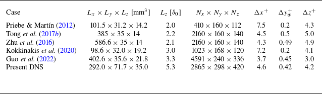



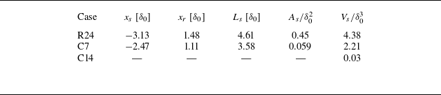
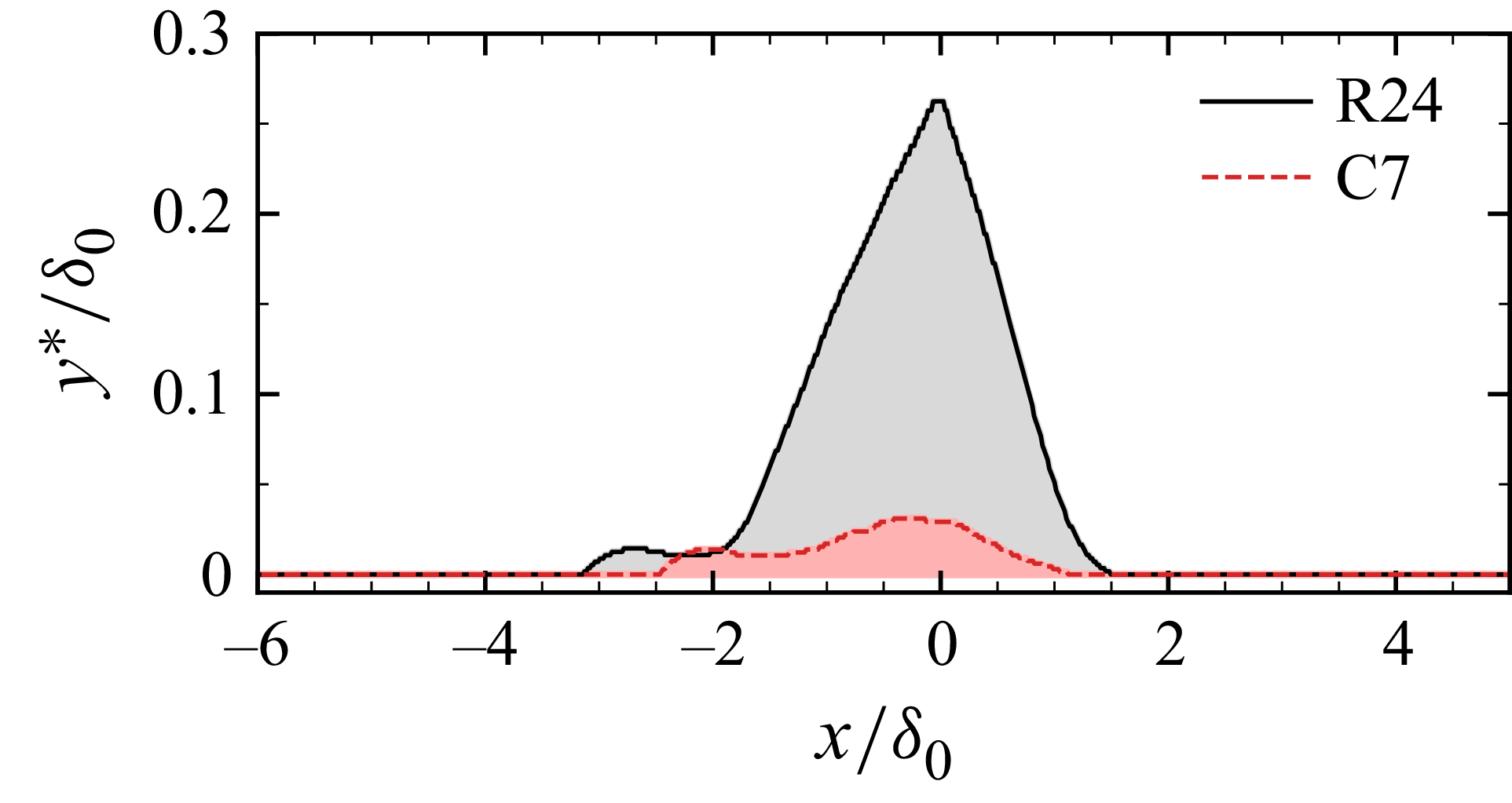


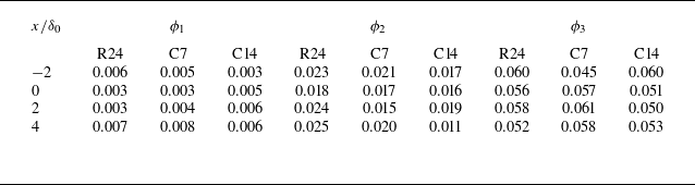


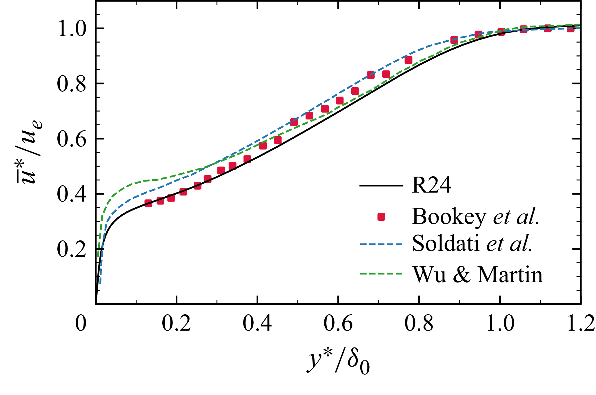

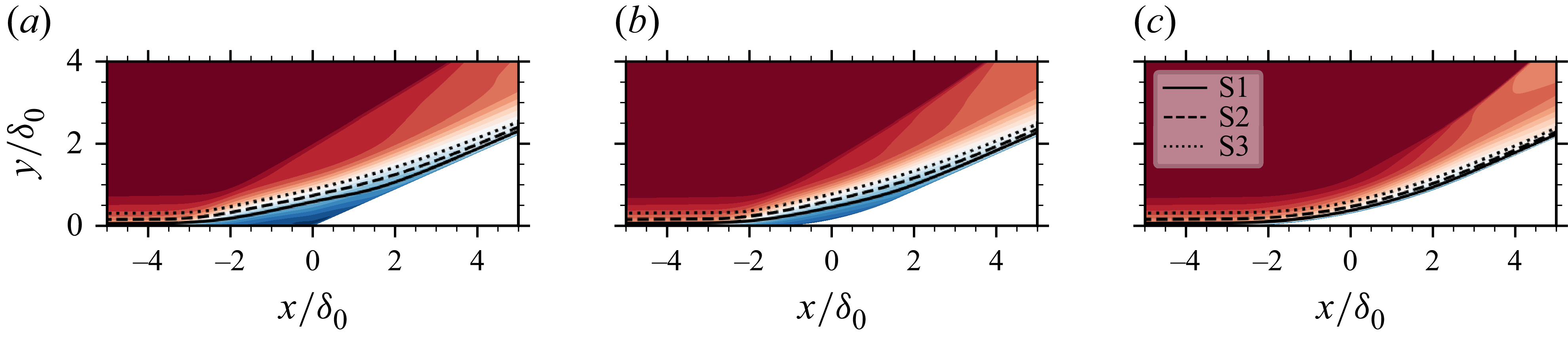


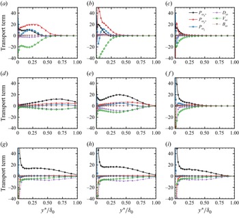


 Open access

