


Impact Statement
The impact of aerosol injections as potential solar climate intervention strategies is poorly understood due to largely unobserved aerosol–cloud interactions. One of few observable examples is temporary cloud trails produced by ship-emitted aerosols. This work focuses on mathematically modeling satellite observations of ship-induced aerosol injections and leveraging it to learn underlying parameters characterizing their behavior.
1. Introduction
For decades, satellite imagery has been able to detect ship tracks, temporary cloud trails created via cloud seeding by emitted aerosols of large ships traversing our oceans. Ship tracks are of interest because they are unintentional and observable examples of marine cloud brightening, a potential solar climate intervention (e.g., Latham, Reference Latham1990; Gunnar et al., Reference Myhre, Shindell, Bréon, Collins, Fuglestvedt, Huang, Koch, Lamarque, Lee, Mendoza, Nakajima, Robock, Stephens, Takemura, Zhang, Aamaas, Boucher, Dalsøren, Daniel, Forster, Granier, Haigh, Hodnebrog, Kaplan, Marston, Nielsen, O’Neill, Peters, Pongratz, Prather, Ramaswamy, Roth, Rotstayn, Smith, Stevenson, Vernier, Wild and Young2013; Council, Reference Council2015). Ship tracks portray the ability of anthropogenic aerosols to perturb boundary layer clouds enough to alter the albedo of the atmosphere, usually brightening the surrounding clouds (Twomey Effect, Twomey et al., Reference Twomey, Howell and Wojciechowski1966; Diamond et al., Reference Diamond, Director, Eastman, Possner and Wood2020), and thus contribute to indirect radiative forcing (Capaldo et al., Reference Capaldo, Corbett, Kasibhatla, Fischbeck and Pandis1999; Eyring et al., Reference Eyring, Isaksen, Berntsen, Collins, Corbett, Endresen, Grainger, Moldanova, Schlager and Stevenson2010). This phenomenon has become more frequently observed as satellite technology has significantly improved since ship tracks were first observed by Conover (Reference Conover1966) and Twomey et al. (Reference Twomey, Howell and Wojciechowski1966). Using the recently deployed GOES-R geostationary satellite series,Footnote 1 tracks have been observed in the atmosphere throughout the year, sometimes persisting more than 24 hr before mixing back into the atmosphere.
Although ship tracks have been actively studied since the 1960s, indirect radiative forcing, amongst other differences to cloud properties, contribute to the largest sources of uncertainty regarding overall radiative forcing in climate models (Carslaw et al., Reference Carslaw, Lee, Reddington, Pringle, Rap, Forster, Mann, Spracklen, Woodhouse, Regayre and Pierce2013). Current understanding of the specific cloud effects from aerosol injections comes from physical simulations under pristine conditions, not representing reality. In climate simulations of this phenomenon, aerosol injections are initiated by the user at a known location in fully defined environments (Wang et al., Reference Wang, Rasch and Feingold2011; Berner et al., Reference Berner, Bretherton and Wood2015; Blossey et al., Reference Blossey, Bretherton, Thornton and Verts2018; Possner et al., Reference Possner, Wang, Wood, Caldeira and Ackerman2018). Satellite-observed tracks, however, form in complex dynamic environments that are challenging and expensive to replicate in physical simulations.
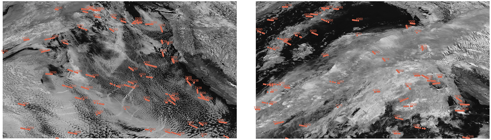
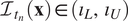
Inferring track behavior from observations comes with many challenges. Track visibility and persistence are highly dependent on atmospheric conditions (Possner et al., Reference Possner, Wang, Wood, Caldeira and Ackerman2018) and inconsistent data availability can also cause tracks to be poorly observed. Due to complex atmosphere dynamics along with variations in fuel types and concentrations, not all emission bursts will produce visible tracks (see Figure 1). Interruptions in the visibility of an existing ship track can occur when ships pass under different atmospheric conditions. Further, vertical transport of the aerosols between the ship’s smoke stack and the boundary clouds is largely unknown and unobserved. The exact altitude of the boundary clouds in which ship tracks are visible and the time lag between an aerosol burst released from a ship, largely depends on complex weather and cloud dynamics. While the height can be approximated using satellite retrieval or reanalysis products, the time lag is difficult to infer from satellite images whose spatial resolution is greater than a kilometer. To the naked eye, new ship track observations appear in images directly above known ship locations due to the imaging resolution. Hence, it is reasonable to assume that the vertical transport path from ship to boundary layer occurs at the same latitude/longitude. We thus implicitly impose a known time lag between ship emissions and their first detection.
Visible ship tracks (left) on April 12, 2019, compared with no visible tracks (right) on April 7, 2019, with 3 hr of known ship locations (shown in red). Images (
 $ 5,000 $
km ×
$ 5,000 $
km ×
 $ 3,000 $
km) taken at 12:00 GMT with ABI spectral band C06 off the coast of California.
$ 3,000 $
km) taken at 12:00 GMT with ABI spectral band C06 off the coast of California.
In this work, we present a computationally efficient, statistical approach to emulating and learning the observed formation and behavior of ship tracks, based upon an advection–diffusion model. Aerosol diffusion models are either driven by the chemical evolution of aerosol composition (e.g., Riemer et al., Reference Riemer, West, Zaveri and Easter2008; Sofiev et al., Reference Sofiev, Sofieva, Elperin, Kleeorin, Rogachevskii and Zilitinkevich2009) or rely upon physical intuition and/or numerical discretization for evaluating a diffusion coefficient (e.g., Stein et al., Reference Stein, Draxler, Rolph, Stunder, Cohen and Ngan2015; Wang et al., Reference Wang, Wang, Easter, Zhang, Ma, Singh, Zhang, Ganguly, Rasch, Burrows, Ghan, Lou, Qian, Yang, Feng, Flanner, Ruby Leung, Liu, Shrivastava, Sun, Tang, Xie and Yoon2020). These methods, however, are validated using limited data collected by targeted campaigns leading to high model sensitivity to cloud and aerosol properties. To the best of our knowledge, few attempts have been made to simulate direct aerosol injections in nonpristine modeling environments, limiting our ability to drive down the known model uncertainties. Importantly, our approach’s ability to learn underlying parameters from observations highlights the power of passively observed data. Specifically, applying our approach to simulated data under controlled settings will enable studying cloud changes from track formation in imagery.
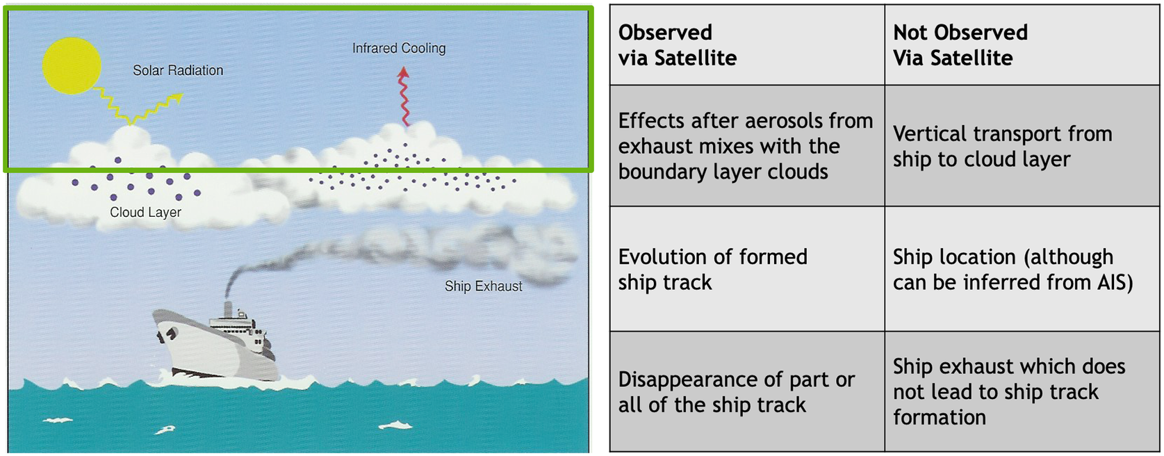
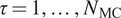
For a given ship, we consider modeling each aerosol emission burst as a single target and assume the ship is continuously emitting bursts. Each target is transported vertically from the ship through the atmosphere until it reaches a specific altitude near the cloud top height at which the target can become visible to orbital satellites and form linear tracks in a cloud. Ship track formations will then move with wind dynamics, a variable that is straightforward to simulate and is independent of ship movement. The visible tracks then persist in the clouds for an unknown time as ship tracks, until the aerosols are fully diffused into the atmosphere and are no longer distinguishable from the surrounding clouds. Figure 2 outlines the general behaviors of the aerosols that are (un)observed via satellite. In this figure, the green box represents the portion of the track formation process that is visible via satellite.
Observable and unobservable behaviors of aerosol emissions from satellite sensors (image available at https://ral.ucar.edu/staff/jwolff/aerosols.html/intro.html).
The remainder of this paper is organized as follows. Section 2 outlines our emulation approach. Section 3 discusses parameter learning. Section 4 provides simulated examples. Lastly, Section 5 considers the potential impacts of this research and directions for future work.
2. Modeling Aerosols Using a Hidden Markov Model
To model the formation and behavior of the aerosol tracks, we construct a state-space point process model relating imaging observations of ship tracks to true aerosol emission bursts.
2.1. State-space representation
The true emission path is generated by continuously emitted aerosol emission bursts or particles by a single ship over the spatial window
 $ \mathcal{X}\subset {\mathrm{\mathbb{R}}}^2 $
up to time
$ \mathcal{X}\subset {\mathrm{\mathbb{R}}}^2 $
up to time
 $ t\in \left[0,N\Delta \right] $
where
$ t\in \left[0,N\Delta \right] $
where
 $ N $
is the number of frames and
$ N $
is the number of frames and
 $ \Delta >0 $
is the time between frames
$ \Delta >0 $
is the time between frames
 $ n $
and
$ n $
and
 $ n+1 $
(typically between 5 and 15 min). A (Lagrangian) particle here is a mathematical object that carries mass in space at a specific time; it models a group of aerosol molecules with distinct mass. The unobserved spatio-temporal point process denoted
$ n+1 $
(typically between 5 and 15 min). A (Lagrangian) particle here is a mathematical object that carries mass in space at a specific time; it models a group of aerosol molecules with distinct mass. The unobserved spatio-temporal point process denoted
 $ \left\{{X}_{t_n}:\left(x,y,{t}_n\right)\in {\mathrm{\mathbb{R}}}^2\times \mathrm{\mathbb{R}}\right\} $
characterizes the set of unknown cardinality and true positions of aerosol emission particles, continuously released prior to (and still visible at) time
$ \left\{{X}_{t_n}:\left(x,y,{t}_n\right)\in {\mathrm{\mathbb{R}}}^2\times \mathrm{\mathbb{R}}\right\} $
characterizes the set of unknown cardinality and true positions of aerosol emission particles, continuously released prior to (and still visible at) time
 $ {t}_n $
. The observed point process
$ {t}_n $
. The observed point process
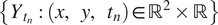 $ \left\{{Y}_{t_n}:\left(x,y,{t}_n\right)\in {\mathrm{\mathbb{R}}}^2\times \mathrm{\mathbb{R}}\right\} $
characterizes positions in satellite imagery containing observed ship tracks in image frame
$ \left\{{Y}_{t_n}:\left(x,y,{t}_n\right)\in {\mathrm{\mathbb{R}}}^2\times \mathrm{\mathbb{R}}\right\} $
characterizes positions in satellite imagery containing observed ship tracks in image frame
 $ n $
generated by
$ n $
generated by
 $ {X}_{t_n} $
. For ship
$ {X}_{t_n} $
. For ship
 $ k=1\dots K $
which produces a track, we assume that its entire emission path is comprised of
$ k=1\dots K $
which produces a track, we assume that its entire emission path is comprised of
 $ {P}_k>0 $
aerosol particles, all of which reach the boundary layer clouds. Assuming that only
$ {P}_k>0 $
aerosol particles, all of which reach the boundary layer clouds. Assuming that only
 $ {k}_{t_n} $
of
$ {k}_{t_n} $
of
 $ K $
ships have entered the window
$ K $
ships have entered the window
 $ \mathcal{X} $
by time
$ \mathcal{X} $
by time
 $ {t}_n<T $
, for an arbitrary single track
$ {t}_n<T $
, for an arbitrary single track
 $ k\le {k}_{t_n} $
, only
$ k\le {k}_{t_n} $
, only
 $ {p}_k\le {P}_k $
particles are expected to become visible. We denote the unobserved point process of true particle positions at time
$ {p}_k\le {P}_k $
particles are expected to become visible. We denote the unobserved point process of true particle positions at time
 $ {t}_n $
as
$ {t}_n $
as
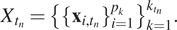 $ {X}_{t_n}={\left\{{\left\{{\mathbf{x}}_{i,{t}_n}\right\}}_{i=1}^{p_k}\right\}}_{k=1}^{k_{t_n}}. $
Existing ship tracks are modified at the next time step
 $ {t}_{n+1} $
in three possible ways: The oldest aerosol emissions at the end of the track diffuse completely and mix back into the atmosphere (leaving no detectable trace), surviving particles diffuse and become less distinguishable as part of the track, and new particles appear at the front of the track in the direction of ship movement. These situations result in
$ {t}_{n+1} $
in three possible ways: The oldest aerosol emissions at the end of the track diffuse completely and mix back into the atmosphere (leaving no detectable trace), surviving particles diffuse and become less distinguishable as part of the track, and new particles appear at the front of the track in the direction of ship movement. These situations result in
 $ {p}_{k_{t_{n+1}}} $
new locations
$ {p}_{k_{t_{n+1}}} $
new locations
 $ {\left\{{\mathbf{x}}_{i,{t}_{n+1}}\right\}}_{i=1}^{p_{k_{t_{n+1}}}} $
in each of the new and existing emission tracks at
$ {\left\{{\mathbf{x}}_{i,{t}_{n+1}}\right\}}_{i=1}^{p_{k_{t_{n+1}}}} $
in each of the new and existing emission tracks at
 $ {t}_{n+1} $
. In practice, the full lifespan (from the first appearance to permanent disappearance) of each emission particle is unknown. Instead, at each observed image frame
$ {t}_{n+1} $
. In practice, the full lifespan (from the first appearance to permanent disappearance) of each emission particle is unknown. Instead, at each observed image frame
 $ n $
, a partial observation of the track within surrounding clouds is captured by the satellite sensor without information on the age of its particles. For track
$ n $
, a partial observation of the track within surrounding clouds is captured by the satellite sensor without information on the age of its particles. For track
 $ {k}_{t_n} $
, therefore, a set of
$ {k}_{t_n} $
, therefore, a set of
 $ {o}_{k_{t_n}}\le {p}_{k_{t_n}} $
observations
$ {o}_{k_{t_n}}\le {p}_{k_{t_n}} $
observations
 $ {Y}_{t_n}={\left\{{\left\{{\mathbf{y}}_{i,{t}_n}\right\}}_{i=1}^{o_k}\right\}}_{k=1}^{k_{t_n}} $
is recorded, where
$ {Y}_{t_n}={\left\{{\left\{{\mathbf{y}}_{i,{t}_n}\right\}}_{i=1}^{o_k}\right\}}_{k=1}^{k_{t_n}} $
is recorded, where
 $ {\mathbf{y}}_{i,{t}_n}\in \mathcal{X} $
.
$ {\mathbf{y}}_{i,{t}_n}\in \mathcal{X} $
.
At time
 $ {t}_n $
, a newly observed track can be generated from newly released emission particles from a new ship. Due to complex atmospheric dynamics, it is not often possible to link new observations to a source; an observed track is not always visible directly above a ship. Thus, we assume that there is no information about which emission particle generates which observation. We now specify a simulation model
$ {t}_n $
, a newly observed track can be generated from newly released emission particles from a new ship. Due to complex atmospheric dynamics, it is not often possible to link new observations to a source; an observed track is not always visible directly above a ship. Thus, we assume that there is no information about which emission particle generates which observation. We now specify a simulation model
 $ {\mathcal{M}}_{\boldsymbol{\theta}} $
relating states
$ {\mathcal{M}}_{\boldsymbol{\theta}} $
relating states
 $ {\left\{{X}_{t_i}\right\}}_{i=1}^N $
from their observation sets
$ {\left\{{X}_{t_i}\right\}}_{i=1}^N $
from their observation sets
 $ {\left\{{Y}_{t_i}\right\}}_{i=1}^N $
generated by parameters
$ {\left\{{Y}_{t_i}\right\}}_{i=1}^N $
generated by parameters
 $ \boldsymbol{\theta} $
.
$ \boldsymbol{\theta} $
.
2.1.1. Multitarget state model
First, we define the three cycles of an aerosol particle: survival ensuing motion and diffusion through the atmosphere, birth of new particles and death, a particle’s permanent disappearance.
After an aerosol track has already formed at time
 $ {t}_{n-1} $
, if an arbitrary associated emission particle
$ {t}_{n-1} $
, if an arbitrary associated emission particle
 $ {\mathbf{x}}_{t_{n-1}}\in {X}_{t_{n-1}} $
survives to time
$ {\mathbf{x}}_{t_{n-1}}\in {X}_{t_{n-1}} $
survives to time
 $ {t}_n>{t}_{n-1} $
, its subsequent state is determined by a drift function which is described by the wind velocity
$ {t}_n>{t}_{n-1} $
, its subsequent state is determined by a drift function which is described by the wind velocity
 $ \mu \left({\mathbf{x}}_{t_{n-1}}\right) $
at
$ \mu \left({\mathbf{x}}_{t_{n-1}}\right) $
at
 $ {\mathbf{x}}_{t_{n-1}} $
, and a diffusion term
$ {\mathbf{x}}_{t_{n-1}} $
, and a diffusion term
 $ \sigma \left({\mathbf{x}}_t\right) $
which describes the diffusion of the emission particle within the clouds it is situated in. This evolution describes a Markov diffusion process and is described by the (continuous time) stochastic partial differential equation (SPDE):
$ \sigma \left({\mathbf{x}}_t\right) $
which describes the diffusion of the emission particle within the clouds it is situated in. This evolution describes a Markov diffusion process and is described by the (continuous time) stochastic partial differential equation (SPDE):
 $$ d{\mathbf{x}}_t=\mu \left({\mathbf{x}}_t,t\right) dt+\sigma \left({\mathbf{x}}_t\right){dB}_t, $$
where
 $ {B}_t\sim {\mathcal{N}}_2\left(\mathbf{0},t{\unicode{x1D540}}_2\right) $
denotes a standard Brownian motion in two dimensions, with
$ {B}_t\sim {\mathcal{N}}_2\left(\mathbf{0},t{\unicode{x1D540}}_2\right) $
denotes a standard Brownian motion in two dimensions, with
 $ {\unicode{x1D540}}_2 $
denoting the 2-dimensional identity matrix. While the drift (wind velocity) is generally known, the diffusion function
$ {\unicode{x1D540}}_2 $
denoting the 2-dimensional identity matrix. While the drift (wind velocity) is generally known, the diffusion function
 $ \sigma \left({\mathbf{x}}_t\right)\equiv {\sigma}_x $
is set to be an unknown constant that describes the diffusivity of an aerosol parcel within the atmospheric boundary layer, and is to be learned from data. To avoid solving (1) with computationally expensive numerical methods, we assume that
$ \sigma \left({\mathbf{x}}_t\right)\equiv {\sigma}_x $
is set to be an unknown constant that describes the diffusivity of an aerosol parcel within the atmospheric boundary layer, and is to be learned from data. To avoid solving (1) with computationally expensive numerical methods, we assume that
 $ \Delta $
is taken small enough so that the wind velocity within each interval
$ \Delta $
is taken small enough so that the wind velocity within each interval
 $ {I}_n:= \left(n\Delta, \left(n+1\right)\Delta \right]\;n\in {\mathrm{\mathbb{Z}}}^{+} $
is approximately constant. With this and given state
$ {I}_n:= \left(n\Delta, \left(n+1\right)\Delta \right]\;n\in {\mathrm{\mathbb{Z}}}^{+} $
is approximately constant. With this and given state
 $ {\mathbf{x}}_s $
at
$ {\mathbf{x}}_s $
at
 $ s\in {I}_n $
, the SPDE
$ s\in {I}_n $
, the SPDE
 $ d{\mathbf{x}}_t=\mu \left({\mathbf{x}}_t\right) dt+{\sigma}_x{dB}_t $
for
$ d{\mathbf{x}}_t=\mu \left({\mathbf{x}}_t\right) dt+{\sigma}_x{dB}_t $
for
 $ s<t\in {I}_n $
, can be solved via
$ s<t\in {I}_n $
, can be solved via
 $ {\mathbf{x}}_t-{\mathbf{x}}_s={\int}_s^t\mu \left({\mathbf{x}}_t\right)\;\mathrm{d}w+{\sigma}_x\left({B}_t-{B}_s\right) $
,
$ {\mathbf{x}}_t-{\mathbf{x}}_s={\int}_s^t\mu \left({\mathbf{x}}_t\right)\;\mathrm{d}w+{\sigma}_x\left({B}_t-{B}_s\right) $
,
 $$ {\mathbf{x}}_t-{\mathbf{x}}_s=\mu \left({\mathbf{x}}_t\right)\left(t-s\right)+{\sigma}_x{B}_{t-s}\hskip5em {B}_{t-s}\sim {\mathcal{N}}_2\left(\mathbf{0},\left(t-s\right){\unicode{x1D540}}_2\right). $$
In particular, the particle’s transition density from
 $ {\mathbf{x}}_{t_{n-1}} $
to
$ {\mathbf{x}}_{t_{n-1}} $
to
 $ {\mathbf{x}}_{t_n} $
is given by
$ {\mathbf{x}}_{t_n} $
is given by
 $ {f}_{t_n\mid {t}_{n-1}}^M\left({\mathbf{x}}_{t_n}|{\mathbf{x}}_{t_{n-1}}\right)={\mathcal{N}}_2\left({\mathbf{x}}_{t_{n-1}}+\mu \left({\mathbf{x}}_{t_{n-1}}\right)\Delta, {\sigma}_x^2\Delta {\unicode{x1D540}}_2\right) $
, modeled by the point process
$ {f}_{t_n\mid {t}_{n-1}}^M\left({\mathbf{x}}_{t_n}|{\mathbf{x}}_{t_{n-1}}\right)={\mathcal{N}}_2\left({\mathbf{x}}_{t_{n-1}}+\mu \left({\mathbf{x}}_{t_{n-1}}\right)\Delta, {\sigma}_x^2\Delta {\unicode{x1D540}}_2\right) $
, modeled by the point process
 $ {S}_{t_n\mid {t}_{n-1}}\left({\mathbf{x}}_{t_{n-1}}\right) $
,
$ {S}_{t_n\mid {t}_{n-1}}\left({\mathbf{x}}_{t_{n-1}}\right) $
,
 $$ {S}_{t_n\mid {t}_{n-1}}\left({\mathbf{x}}_{t_{n-1}}\right)=\left\{\begin{array}{ll}{\mathbf{x}}_{t_n}& \mathrm{where}\;{\mathbf{x}}_{t_n}\sim {f}_{t_n\mid {t}_{n-1}}^M\left(\cdot |{\mathbf{x}}_{t_{n-1}}\right)\;\mathrm{with}\ \mathrm{probability}\;{p}_{S,{t}_n}\left({b}_{{\mathbf{x}}_{t_{n-1}}}\right)\\ {}\varnothing & \mathrm{otherwise},\end{array}\right. $$
where
 $ {p}_{S,{t}_n}\left({b}_{{\mathbf{x}}_{t_{n-1}}}\right) $
denotes the probability that particle
$ {p}_{S,{t}_n}\left({b}_{{\mathbf{x}}_{t_{n-1}}}\right) $
denotes the probability that particle
 $ {\mathbf{x}}_{t_{n-1}} $
will survive (be visually trackable) at
$ {\mathbf{x}}_{t_{n-1}} $
will survive (be visually trackable) at
 $ {t}_n $
.
$ {t}_n $
.
A new emission particle at time
 $ {t}_n\in \mathrm{\mathbb{R}} $
can arise either as a spontaneous birth (of a newly risen emission) independent of any existing tracks, or via spawning from an existing emission source (e.g., at the head of an existing track), resulting in a newly visible emission particle. The birth time of particle
$ {t}_n\in \mathrm{\mathbb{R}} $
can arise either as a spontaneous birth (of a newly risen emission) independent of any existing tracks, or via spawning from an existing emission source (e.g., at the head of an existing track), resulting in a newly visible emission particle. The birth time of particle
 $ {\mathbf{x}}_{t_n} $
observed at time
$ {\mathbf{x}}_{t_n} $
observed at time
 $ {t}_n $
is denoted
$ {t}_n $
is denoted
 $ {b}_{\mathbf{x}} $
. Spontaneous births at time
$ {b}_{\mathbf{x}} $
. Spontaneous births at time
 $ t $
are denoted by the finite point process
$ t $
are denoted by the finite point process
 $ {\Gamma}_t $
, modeled as a Poisson point process (Maher, Reference Mahler2007) with intensity function
$ {\Gamma}_t $
, modeled as a Poisson point process (Maher, Reference Mahler2007) with intensity function
 $ {\gamma}_t\left(\mathbf{x}\right)={\lambda}_{\gamma_t}\hskip0.35em {f}_{b,t}\left(\mathbf{x}\right) $
, where for
$ {\gamma}_t\left(\mathbf{x}\right)={\lambda}_{\gamma_t}\hskip0.35em {f}_{b,t}\left(\mathbf{x}\right) $
, where for
 $ \mathbf{x}\in \mathcal{X},\hskip0.35em {\Gamma}_t\sim \mathrm{Poisson}\left({\lambda}_{\gamma_t}\hskip0.35em {f}_{b,\hskip0.35em t}\left(\mathbf{x}\right)\right) $
. Here,
$ \mathbf{x}\in \mathcal{X},\hskip0.35em {\Gamma}_t\sim \mathrm{Poisson}\left({\lambda}_{\gamma_t}\hskip0.35em {f}_{b,\hskip0.35em t}\left(\mathbf{x}\right)\right) $
. Here,
 $ {N}_{b,\hskip0.35em t}\sim \mathrm{Poisson}\left({\int}_{\mathcal{X}}{\lambda}_{\gamma_t}\hskip0.35em {f}_{b,\hskip0.35em t}\left(\mathbf{x}\right)\mathrm{d}\mathbf{x}\right) $
denotes the number of births occurring in
$ {N}_{b,\hskip0.35em t}\sim \mathrm{Poisson}\left({\int}_{\mathcal{X}}{\lambda}_{\gamma_t}\hskip0.35em {f}_{b,\hskip0.35em t}\left(\mathbf{x}\right)\mathrm{d}\mathbf{x}\right) $
denotes the number of births occurring in
 $ \mathcal{X} $
at time
$ \mathcal{X} $
at time
 $ t $
and
$ t $
and
 $ {f}_{b_t}\left(\mathbf{x}\right) $
denotes their spatial distribution. We may assume that if
$ {f}_{b_t}\left(\mathbf{x}\right) $
denotes their spatial distribution. We may assume that if
 $ {\mathbf{x}}_{b,{t}_n} $
is the position of a new ship at time
$ {\mathbf{x}}_{b,{t}_n} $
is the position of a new ship at time
 $ {t}_n $
, then
$ {t}_n $
, then
 $ {f}_{b_{t_n+{\varepsilon}_b}}\left(\mathbf{x}\right)={\mathcal{N}}_2\left({\mathbf{x}}_{b,{t}_n},{\sigma}_b^2{\unicode{x1D540}}_2\right) $
where
$ {f}_{b_{t_n+{\varepsilon}_b}}\left(\mathbf{x}\right)={\mathcal{N}}_2\left({\mathbf{x}}_{b,{t}_n},{\sigma}_b^2{\unicode{x1D540}}_2\right) $
where
 $ {\varepsilon}_b $
denotes the time lag between ship emission and aerosol observation at the boundary layer. On the other hand, spawned births occurring within
$ {\varepsilon}_b $
denotes the time lag between ship emission and aerosol observation at the boundary layer. On the other hand, spawned births occurring within
 $ {I}_{n-1} $
denote newly visible particles from existing tracks that reach the cloud top layer at time
$ {I}_{n-1} $
denote newly visible particles from existing tracks that reach the cloud top layer at time
 $ {t}_n $
. These can only be spawned by particles birthed in
$ {t}_n $
. These can only be spawned by particles birthed in
 $ \left[{t}_n-{\varepsilon}_b,{t}_n\right] $
, as this models the continuous emission of aerosol particles in a single stream. In this paper, we model the set of spawned births
$ \left[{t}_n-{\varepsilon}_b,{t}_n\right] $
, as this models the continuous emission of aerosol particles in a single stream. In this paper, we model the set of spawned births
 $ {B}_{t_n\mid {t}_{n-1}}\left({\mathbf{x}}_{t_{n-1}}\right) $
at time
$ {B}_{t_n\mid {t}_{n-1}}\left({\mathbf{x}}_{t_{n-1}}\right) $
at time
 $ {t}_n $
from a particle
$ {t}_n $
from a particle
 $ {\mathbf{x}}_{t_{n-1}} $
as a Bernoulli point process (Mahler, Reference Mahler2007):
$ {\mathbf{x}}_{t_{n-1}} $
as a Bernoulli point process (Mahler, Reference Mahler2007):
 $$ {B}_{t_n\mid {t}_{n-1}}\left({\mathbf{x}}_{t_{n-1}}\right)=\left\{\begin{array}{ll}\left\{\mathbf{x}\right\};\mathbf{x}\sim {f}_{t_n\mid {t}_{n-1}}^{\beta}\left(\mathbf{x}|{\mathbf{x}}_{t_{n-1}}\right)\;\mathrm{with}\ \mathrm{probability}\hskip0.8em {p}_{\beta, {t}_n}& \hskip0.8em {t}_{n-2}<{b}_{{\mathbf{x}}_{t_{n-1}}}\le {t}_{n-1}\\ {}\operatorname{}& \mathrm{otherwise}.\end{array}\right. $$
Knowledge of ship positions (e.g., via SeaVisionFootnote
2) when observing tracks being formed, motivates using the spawning density
 $ {f}_{t_n\mid {t}_{n-1}}^{\beta}\left(\mathbf{x}|{\mathbf{x}}_{t_{n-1}}\right)={\mathcal{N}}_2\left({\mathbf{x}}_{b,{t}_n-{\varepsilon}_b},{\sigma}_{\beta}^2{\unicode{x1D540}}_2\right) $
. Since the spawning probability
$ {f}_{t_n\mid {t}_{n-1}}^{\beta}\left(\mathbf{x}|{\mathbf{x}}_{t_{n-1}}\right)={\mathcal{N}}_2\left({\mathbf{x}}_{b,{t}_n-{\varepsilon}_b},{\sigma}_{\beta}^2{\unicode{x1D540}}_2\right) $
. Since the spawning probability
 $ {p}_{\beta, {t}_n} $
is directly related to the number of aerosol particles emitted, for simulation purposes, we assume that each ship continuously emits aerosols in
$ {p}_{\beta, {t}_n} $
is directly related to the number of aerosol particles emitted, for simulation purposes, we assume that each ship continuously emits aerosols in
 $ \mathcal{X} $
up to time
$ \mathcal{X} $
up to time
 $ T=N\Delta $
, enabling
$ T=N\Delta $
, enabling
 $ {p}_{\beta, {t}_n}=\unicode{x1D7D9}\left({t}_n\le T\right) $
.
$ {p}_{\beta, {t}_n}=\unicode{x1D7D9}\left({t}_n\le T\right) $
.
Given
 $ {X}_{t_{n-1}} $
at time
$ {X}_{t_{n-1}} $
at time
 $ {t}_{n-1} $
, each particle
$ {t}_{n-1} $
, each particle
 $ \mathbf{x}\in {X}_{t_{n-1}} $
with birth time
$ \mathbf{x}\in {X}_{t_{n-1}} $
with birth time
 $ {b}_{\mathbf{x}} $
, either continues to be visually trackable to
$ {b}_{\mathbf{x}} $
, either continues to be visually trackable to
 $ {t}_n $
with probability
$ {t}_n $
with probability
 $ {p}_{S,{t}_n}\left({b}_{\mathbf{x}}\right) $
, or “dies” with probability
$ {p}_{S,{t}_n}\left({b}_{\mathbf{x}}\right) $
, or “dies” with probability
 $ 1-{p}_{S,{t}_n}\left({b}_{\mathbf{x}}\right) $
. Here, a “death” of an emission particle occurs when it sinks back through the atmosphere and ceases to be visible. Further, its survival probability is solely a function of its persistence time, since the effects of up and downward drafts in the atmosphere on each particle render spatial effects negligible. We assume that each ship produces a cloud–aeorosol track that has an average lifetime
$ 1-{p}_{S,{t}_n}\left({b}_{\mathbf{x}}\right) $
. Here, a “death” of an emission particle occurs when it sinks back through the atmosphere and ceases to be visible. Further, its survival probability is solely a function of its persistence time, since the effects of up and downward drafts in the atmosphere on each particle render spatial effects negligible. We assume that each ship produces a cloud–aeorosol track that has an average lifetime
 $ {T}_d\sim \mathrm{Exp}\left({\lambda}_T\right) $
from birth. Given
$ {T}_d\sim \mathrm{Exp}\left({\lambda}_T\right) $
from birth. Given
 $ {T}_d $
, individual aerosol particles contained in its emission then each have an independently and identically distributed (i.i.d.) death time
$ {T}_d $
, individual aerosol particles contained in its emission then each have an independently and identically distributed (i.i.d.) death time
 $ d\sim \mathrm{Log}-\mathrm{normal}\Big({\mu}_d=\log {T}_d{\left({\sigma}_{p_d}^2+{T}_d^2\right)}^{-1/2},\hskip0.5em {\sigma}_d^2=\log \left({\sigma}_{p_d}^2+{T}_d^2\right)/{T}_d^2, $
where
$ d\sim \mathrm{Log}-\mathrm{normal}\Big({\mu}_d=\log {T}_d{\left({\sigma}_{p_d}^2+{T}_d^2\right)}^{-1/2},\hskip0.5em {\sigma}_d^2=\log \left({\sigma}_{p_d}^2+{T}_d^2\right)/{T}_d^2, $
where
 $ {\sigma}_{p_d}^2 $
is the variance of particle death time, a fixed simulation input requiring estimation from data.
$ {\sigma}_{p_d}^2 $
is the variance of particle death time, a fixed simulation input requiring estimation from data.
Altogether, we have
 $ {X}_{t_n}=\left[{\cup}_{\mathbf{x}\in {X}_{t_{n-1}}}{S}_{t_n\mid {t}_{n-1}}\left(\mathbf{x}\right)\right]\cup \left[{\cup}_{\mathbf{x}\in {X}_{t_{n-1}}}{B}_{t_n\mid {t}_{n-1}}\left(\mathbf{x}\right)\right]\cup {\Gamma}_{t_n} $
over independent unions.
$ {X}_{t_n}=\left[{\cup}_{\mathbf{x}\in {X}_{t_{n-1}}}{S}_{t_n\mid {t}_{n-1}}\left(\mathbf{x}\right)\right]\cup \left[{\cup}_{\mathbf{x}\in {X}_{t_{n-1}}}{B}_{t_n\mid {t}_{n-1}}\left(\mathbf{x}\right)\right]\cup {\Gamma}_{t_n} $
over independent unions.
2.1.2. Multitarget observational model
Here, we describe a finite point process model for the time evolution of the set
 $ {\left\{{Y}_{t_n}\right\}}_{n=1}^N $
generated from emission tracks
$ {\left\{{Y}_{t_n}\right\}}_{n=1}^N $
generated from emission tracks
 $ {\left\{{X}_{t_n}\right\}}_{n=1}^N $
and observed over images
$ {\left\{{X}_{t_n}\right\}}_{n=1}^N $
and observed over images
 $ {\left\{{\mathcal{Y}}_{t_n}\right\}}_{n=1}^N $
.
$ {\left\{{\mathcal{Y}}_{t_n}\right\}}_{n=1}^N $
.
An arbitrary observation
 $ {\mathbf{y}}_{t_n}\in {Y}_{t_n} $
of unknown particle
$ {\mathbf{y}}_{t_n}\in {Y}_{t_n} $
of unknown particle
 $ {\mathbf{x}}_{t_n}\in {X}_{t_n} $
is generated from a Gaussian density centered at
$ {\mathbf{x}}_{t_n}\in {X}_{t_n} $
is generated from a Gaussian density centered at
 $ {\mathbf{x}}_{t_n} $
, with covariance taken to be the marginal covariance of
$ {\mathbf{x}}_{t_n} $
, with covariance taken to be the marginal covariance of
 $ {\mathbf{x}}_{t_n} $
. Its marginal density can be calculated via
$ {\mathbf{x}}_{t_n} $
. Its marginal density can be calculated via
 $ f\left({\mathbf{x}}_{t_n}\right)={\int}_{\mathcal{X}}{f}_{t_n\mid {b}_{\mathbf{x}}}^M\left({\mathbf{x}}_{t_n}|{\mathbf{x}}_{b_{\mathbf{x}}}\right)\pi \left({\mathbf{x}}_{b_{\mathbf{x}}}\right)\;\mathrm{d}{\mathbf{x}}_{b_{\mathbf{x}}} $
with
$ f\left({\mathbf{x}}_{t_n}\right)={\int}_{\mathcal{X}}{f}_{t_n\mid {b}_{\mathbf{x}}}^M\left({\mathbf{x}}_{t_n}|{\mathbf{x}}_{b_{\mathbf{x}}}\right)\pi \left({\mathbf{x}}_{b_{\mathbf{x}}}\right)\;\mathrm{d}{\mathbf{x}}_{b_{\mathbf{x}}} $
with
 $ \pi \left({\mathbf{x}}_{b_{\mathbf{x}}}\right) $
being the initial probability density of particle
$ \pi \left({\mathbf{x}}_{b_{\mathbf{x}}}\right) $
being the initial probability density of particle
 $ {\mathbf{x}}_{t_n} $
at the time of its birth. In this paper, we take
$ {\mathbf{x}}_{t_n} $
at the time of its birth. In this paper, we take
 $ \pi \left({\mathbf{x}}_{b_{\mathbf{x}}}\right)=\delta \left({\mathbf{x}}_{b_{\mathbf{x}}}\right) $
, the dirac delta function centered at
$ \pi \left({\mathbf{x}}_{b_{\mathbf{x}}}\right)=\delta \left({\mathbf{x}}_{b_{\mathbf{x}}}\right) $
, the dirac delta function centered at
 $ {\mathbf{x}}_{b_{\mathbf{x}}} $
, yielding
$ {\mathbf{x}}_{b_{\mathbf{x}}} $
, yielding
 $ {\mathbf{y}}_{t_n}\mid {\mathbf{x}}_{t_n}\sim {\mathcal{N}}_2\left({\mathbf{x}}_{t_n},{\sigma}_x^2\left({t}_n-{b}_{\mathbf{x}}\right){\unicode{x1D540}}_2\right). $
For image observations, we discretize this such that the pixel intensity of a pixel
$ {\mathbf{y}}_{t_n}\mid {\mathbf{x}}_{t_n}\sim {\mathcal{N}}_2\left({\mathbf{x}}_{t_n},{\sigma}_x^2\left({t}_n-{b}_{\mathbf{x}}\right){\unicode{x1D540}}_2\right). $
For image observations, we discretize this such that the pixel intensity of a pixel
 $ {\mathcal{Y}}_{t_n}(P) $
, denoted
$ {\mathcal{Y}}_{t_n}(P) $
, denoted
 $ {\mathcal{I}}_{t_n}(P) $
, follows
$ {\mathcal{I}}_{t_n}(P) $
, follows
 $ {\mathcal{I}}_{t_n}(P)\propto {\sum}_{\mathbf{x}\in {X}_{t_n}}{\int}_P\hskip0.35em f\left(\mathbf{y}|\mathbf{x}\right)\mathrm{d}\mathbf{y} $
with normalization constant given by the highest pixel intensity across the video.
$ {\mathcal{I}}_{t_n}(P)\propto {\sum}_{\mathbf{x}\in {X}_{t_n}}{\int}_P\hskip0.35em f\left(\mathbf{y}|\mathbf{x}\right)\mathrm{d}\mathbf{y} $
with normalization constant given by the highest pixel intensity across the video.
A particle
 $ \mathbf{x}\in {X}_t $
, at time
$ \mathbf{x}\in {X}_t $
, at time
 $ t $
is only detected by a satellite sensor with probability
$ t $
is only detected by a satellite sensor with probability
 $ {p}_{D,\hskip0.35em t}\left(\mathbf{x}\right) $
. This detection probability has a spatio-temporal dependence structure which is needed to first, model the spatial randomness of cloud humidity and second, to account for cloud movement across
$ {p}_{D,\hskip0.35em t}\left(\mathbf{x}\right) $
. This detection probability has a spatio-temporal dependence structure which is needed to first, model the spatial randomness of cloud humidity and second, to account for cloud movement across
 $ \mathcal{X} $
. If the cloud humidity is too low or too high, emission particles cannot be detected. In the former case, particles cannot be observed since clouds cannot form to produce the necessary observations. In the latter, the cloud density may be too high, or may already be contaminated with existing aerosols which would subsequently not produce observations of new particles. To deal with this, we choose to model
$ \mathcal{X} $
. If the cloud humidity is too low or too high, emission particles cannot be detected. In the former case, particles cannot be observed since clouds cannot form to produce the necessary observations. In the latter, the cloud density may be too high, or may already be contaminated with existing aerosols which would subsequently not produce observations of new particles. To deal with this, we choose to model
 $ {p}_{D,t}\left(\mathbf{x}\right) $
as a function of the existing cloud humidity, formulated by modeling baseline pixel intensities measured by the satellite sensor and utilizing a lower and upper threshold
$ {p}_{D,t}\left(\mathbf{x}\right) $
as a function of the existing cloud humidity, formulated by modeling baseline pixel intensities measured by the satellite sensor and utilizing a lower and upper threshold
 $ {\iota}_L,\hskip0.35em {\iota}_U $
. In particular, setting
$ {\iota}_L,\hskip0.35em {\iota}_U $
. In particular, setting
 $ {p}_{D,{t}_n}\left(\mathbf{x}\right)=1\left({\iota}_L<{\mathcal{I}}_{t_n}\left(\mathbf{x}\right)<{\iota}_U\right) $
, enables a particle to be observed with probability one if its true location
$ {p}_{D,{t}_n}\left(\mathbf{x}\right)=1\left({\iota}_L<{\mathcal{I}}_{t_n}\left(\mathbf{x}\right)<{\iota}_U\right) $
, enables a particle to be observed with probability one if its true location
 $ \mathbf{x} $
lies within a pixel of the
$ \mathbf{x} $
lies within a pixel of the
 $ n $
th frame with an intensity
$ n $
th frame with an intensity
 $ {\mathcal{I}}_{t_n}\left(\mathbf{x}\right)\in \left({\iota}_L,{\iota}_U\right) $
, sufficient for its observation. Subsequently, the observational point process
$ {\mathcal{I}}_{t_n}\left(\mathbf{x}\right)\in \left({\iota}_L,{\iota}_U\right) $
, sufficient for its observation. Subsequently, the observational point process
 $ {\Theta}_{t_n}\left({\mathbf{x}}_{t_n}\right) $
from an emission particle
$ {\Theta}_{t_n}\left({\mathbf{x}}_{t_n}\right) $
from an emission particle
 $ {\mathbf{x}}_{t_n}\in \mathcal{X} $
follows:
$ {\mathbf{x}}_{t_n}\in \mathcal{X} $
follows:
 $$ {\Theta}_{t_n}\left({\mathbf{x}}_{t_n}\right)=\left\{\begin{array}{ll}\left\{\mathbf{y}\right\}\;\mathrm{where}\;\mathbf{y}\sim {\mathbf{y}}_{t_n}\mid {\mathbf{x}}_{t_n}& \mathrm{with}\ \mathrm{probability}\;{p}_{D,{t}_n}\left({\mathbf{x}}_{t_n}\right)\\ {}\varnothing & \mathrm{with}\ \mathrm{probability}\;1-{p}_{D,{t}_n}\left({\mathbf{x}}_{t_n}\right),\end{array}\right. $$
specifying multitarget observations
 $ {Y}_{t_n}={\cup}_{\mathbf{x}\in {X}_{t_n}}{\Theta}_{t_n}\left(\mathbf{x}\right) $
observed within pixelated images
$ {Y}_{t_n}={\cup}_{\mathbf{x}\in {X}_{t_n}}{\Theta}_{t_n}\left(\mathbf{x}\right) $
observed within pixelated images
 $ {\left\{{\mathcal{Y}}_{t_n}\right\}}_{n=1}^N $
.
$ {\left\{{\mathcal{Y}}_{t_n}\right\}}_{n=1}^N $
.
3. Data Assimilation and Parameter Learning
In this section, we discuss a method for data assimilation and learning underlying parameters of the model from satellite observations, based upon the ship track emulation tool proposed here.
The emulation model
 $ {\mathcal{M}}_{\boldsymbol{\theta}} $
comprises of parameters
$ {\mathcal{M}}_{\boldsymbol{\theta}} $
comprises of parameters
 $ \boldsymbol{\theta} $
that require estimation from data. Typical methods of data-driven estimation extend standard filtering approaches (Kalman, Reference Kalman1960) to the point process domain by utilizing cardinalized probability hypothesis density (CPHD) filters (e.g., Vo et al., Reference Vo, Vo and Cantoni2006. These not only allow for efficient estimation of the cardinality and states of the underlying point process but can be leveraged for statistical parameter learning (e.g., Jiang et al., Reference Jiang, Singh and Yıldırım2015). Unfortunately, utilizing filtering approaches for this problem requires extracting the observations
$ \boldsymbol{\theta} $
that require estimation from data. Typical methods of data-driven estimation extend standard filtering approaches (Kalman, Reference Kalman1960) to the point process domain by utilizing cardinalized probability hypothesis density (CPHD) filters (e.g., Vo et al., Reference Vo, Vo and Cantoni2006. These not only allow for efficient estimation of the cardinality and states of the underlying point process but can be leveraged for statistical parameter learning (e.g., Jiang et al., Reference Jiang, Singh and Yıldırım2015). Unfortunately, utilizing filtering approaches for this problem requires extracting the observations
 $ {\left\{{Y}_{t_n}\right\}}_{n=1}^N $
from relatively coarse satellite images with pixels containing overlapping tracks, a highly challenging problem. To alleviate this, we propose accurate simulation-based learning via Sequential Monte Carlo within an Approximate Bayesian Computation (ABC-SMC) approach, described in detail in Toni et al. (Reference Toni, Welch, Strelkowa, Michael and Stumpf2009).
$ {\left\{{Y}_{t_n}\right\}}_{n=1}^N $
from relatively coarse satellite images with pixels containing overlapping tracks, a highly challenging problem. To alleviate this, we propose accurate simulation-based learning via Sequential Monte Carlo within an Approximate Bayesian Computation (ABC-SMC) approach, described in detail in Toni et al. (Reference Toni, Welch, Strelkowa, Michael and Stumpf2009).
ABC-SMC works as follows. At iteration
 $ \tau =0 $
, parameters are sampled from a prior density
$ \tau =0 $
, parameters are sampled from a prior density
 $ {\boldsymbol{\theta}}_j^{(0)}\sim \pi \left(\boldsymbol{\theta} \right) $
until
$ {\boldsymbol{\theta}}_j^{(0)}\sim \pi \left(\boldsymbol{\theta} \right) $
until
 $ M $
datasets
$ M $
datasets
 $ {\mathcal{Y}}^j\sim {\mathcal{M}}_{{\boldsymbol{\theta}}_j^{(0)}} $
are within a tolerance
$ {\mathcal{Y}}^j\sim {\mathcal{M}}_{{\boldsymbol{\theta}}_j^{(0)}} $
are within a tolerance
 $ {\varepsilon}_{\tau } $
of the observed dataset
$ {\varepsilon}_{\tau } $
of the observed dataset
 $ {\mathcal{Y}}^d $
. This is computed over the sequence of images via the chosen distance function
$ {\mathcal{Y}}^d $
. This is computed over the sequence of images via the chosen distance function
 $$ \Delta \left({\mathcal{Y}}^d,{\mathcal{Y}}^j\right)=\sum \limits_{n=1}^N\sum \limits_P{\left({\mathcal{Y}}_n^d(P)-{\mathcal{Y}}_n^j(P)\right)}^2. $$
For
 $ \tau =1,\dots, \hskip0.35em {N}_{\mathrm{MC}} $
, tolerances
$ \tau =1,\dots, \hskip0.35em {N}_{\mathrm{MC}} $
, tolerances
 $ {\varepsilon}_{\tau }<{\varepsilon}_{\tau -1} $
are chosen and
$ {\varepsilon}_{\tau }<{\varepsilon}_{\tau -1} $
are chosen and
 $ {\boldsymbol{\theta}}_j^{\ast}\sim {\left\{{\boldsymbol{\theta}}_m^{\tau -1}\right\}}_{m=1}^M $
sampled with replacement using importance weights
$ {\boldsymbol{\theta}}_j^{\ast}\sim {\left\{{\boldsymbol{\theta}}_m^{\tau -1}\right\}}_{m=1}^M $
sampled with replacement using importance weights
 $ {w}_j^{\left(\tau \right)}=\pi \left({\boldsymbol{\theta}}_j^{\left(\tau \right)}\right)/{\sum}_{n=1}^N{w}_n^{\left(\tau -1\right)}{K}_{\tau}\left({\boldsymbol{\theta}}_j^{\ast }|{\boldsymbol{\theta}}_n^{\left(\tau -1\right)}\right) $
and perturbed via
$ {w}_j^{\left(\tau \right)}=\pi \left({\boldsymbol{\theta}}_j^{\left(\tau \right)}\right)/{\sum}_{n=1}^N{w}_n^{\left(\tau -1\right)}{K}_{\tau}\left({\boldsymbol{\theta}}_j^{\ast }|{\boldsymbol{\theta}}_n^{\left(\tau -1\right)}\right) $
and perturbed via
 $ {K}_{\tau } $
to generate
$ {K}_{\tau } $
to generate
 $ {\boldsymbol{\theta}}_j^{\left(\tau \right)} $
, until
$ {\boldsymbol{\theta}}_j^{\left(\tau \right)} $
, until
 $ M $
datasets
$ M $
datasets
 $ {\mathcal{Y}}^j\sim {\mathcal{M}}_{{\boldsymbol{\theta}}_j^{\left(\tau \right)}} $
satisfy
$ {\mathcal{Y}}^j\sim {\mathcal{M}}_{{\boldsymbol{\theta}}_j^{\left(\tau \right)}} $
satisfy
 $ \Delta \left({\mathcal{Y}}^d,{\mathcal{Y}}^j\right)<{\varepsilon}_{\tau } $
. Parameter values are therefore sequentially updated, enabling the posterior
$ \Delta \left({\mathcal{Y}}^d,{\mathcal{Y}}^j\right)<{\varepsilon}_{\tau } $
. Parameter values are therefore sequentially updated, enabling the posterior
 $ {p}_{\varepsilon_{\tau }}\left(\boldsymbol{\theta} |{\mathcal{Y}}^d\right)\approx {\sum}_{j=1}^M{w}_j^{\left(\tau \right)}\delta \left(\boldsymbol{\theta} -{\boldsymbol{\theta}}_j^{\left(\tau \right)}\right)/M $
at
$ {p}_{\varepsilon_{\tau }}\left(\boldsymbol{\theta} |{\mathcal{Y}}^d\right)\approx {\sum}_{j=1}^M{w}_j^{\left(\tau \right)}\delta \left(\boldsymbol{\theta} -{\boldsymbol{\theta}}_j^{\left(\tau \right)}\right)/M $
at
 $ \tau ={N}_{\mathrm{MC}} $
to be used to infer
$ \tau ={N}_{\mathrm{MC}} $
to be used to infer
 $ \boldsymbol{\theta} $
.
$ \boldsymbol{\theta} $
.
4. Imaging Simulation
Here, we present a ship track emulation example and parameter learning with ABC-SMC.
A snapshot of five simulated images taken 20 time steps apart with time step
 $ \Delta =0.2 $
hr are shown in Figure 3. In this study, four ships were simulated in
$ \Delta =0.2 $
hr are shown in Figure 3. In this study, four ships were simulated in
 $ 300\times 500 $
longitude/latitude units appearing at staggered times. The tracks were generated using ship positions, spawning, persistence, and death processes within a simulated circular wind motion where
$ 300\times 500 $
longitude/latitude units appearing at staggered times. The tracks were generated using ship positions, spawning, persistence, and death processes within a simulated circular wind motion where
 $ \mu \left({\mathbf{x}}_t\right)=10\pi \sqrt{{\left(x-0.2t\right)}^2+{\left(y+0.1t\right)}^2}/4N\Delta $
. An initial realistic cloud background image, where cloud pixels also moved with the simulated wind field, was omitted for illustration purposes. In particular, tracks are observed to follow both the ships’ directions and wind field, with diffusivity emphasized by the broadening of each track through time. Further, pixel intensities are observed to be higher when cloud tracks overlap, highlighting the expected increase in pixel intensity when multiple sources are present.
$ \mu \left({\mathbf{x}}_t\right)=10\pi \sqrt{{\left(x-0.2t\right)}^2+{\left(y+0.1t\right)}^2}/4N\Delta $
. An initial realistic cloud background image, where cloud pixels also moved with the simulated wind field, was omitted for illustration purposes. In particular, tracks are observed to follow both the ships’ directions and wind field, with diffusivity emphasized by the broadening of each track through time. Further, pixel intensities are observed to be higher when cloud tracks overlap, highlighting the expected increase in pixel intensity when multiple sources are present.
Top: Simulation snapshots are taken 4 hr apart, with
 $ N=100 $
,
$ N=100 $
,
 $ \Delta =0.2 $
hr,
$ \Delta =0.2 $
hr,
 $ {\varepsilon}_b=5 $
hr,
$ {\varepsilon}_b=5 $
hr,
 $ {\sigma}_{\beta }={\sigma}_x=0.01 $
,
$ {\sigma}_{\beta }={\sigma}_x=0.01 $
,
 $ {\lambda}_T=80 $
hr,
$ {\lambda}_T=80 $
hr,
 $ {\sigma}_{p_d}=0.2 $
hr,
$ {\sigma}_{p_d}=0.2 $
hr,
 $ {\iota}_L=0.25 $
, and
$ {\iota}_L=0.25 $
, and
 $ {\iota}_U=0.75 $
. Ships (red, blue, purple, and yellow) indicated by colored dotted trajectories have initial conditions
$ {\iota}_U=0.75 $
. Ships (red, blue, purple, and yellow) indicated by colored dotted trajectories have initial conditions
 $ {\mathbf{b}}_t=\left[5\cos \left(\pi t/10N\Delta \right)+3,5\sin \left(\pi t/2N\Delta \right)+2\right],\left[1+5t/N\Delta, 18-2t/N\Delta \right],\left[1+5t/N\Delta, 18-10t/N\Delta \right],\left[-4+10t/N\Delta, 10+2t/N\Delta \right] $
respectively, with heads (orange). Wind direction is shown via yellow arrows and tracks indicated by white trajectories. Bottom: Approximate posterior densities for
$ {\mathbf{b}}_t=\left[5\cos \left(\pi t/10N\Delta \right)+3,5\sin \left(\pi t/2N\Delta \right)+2\right],\left[1+5t/N\Delta, 18-2t/N\Delta \right],\left[1+5t/N\Delta, 18-10t/N\Delta \right],\left[-4+10t/N\Delta, 10+2t/N\Delta \right] $
respectively, with heads (orange). Wind direction is shown via yellow arrows and tracks indicated by white trajectories. Bottom: Approximate posterior densities for
 $ {\theta}_1={\sigma}_{\beta } $
(left) and
$ {\theta}_1={\sigma}_{\beta } $
(left) and
 $ {\theta}_2={\sigma}_x $
(right) are shown with estimated values (red), true values (black), and 95% credible intervals (blue). Here,
$ {\theta}_2={\sigma}_x $
(right) are shown with estimated values (red), true values (black), and 95% credible intervals (blue). Here,
 $ {N}_{\mathrm{MC}}=4 $
,
$ {N}_{\mathrm{MC}}=4 $
,
 $ M=50 $
,
$ M=50 $
,
 $ {\theta}_i\sim \mathrm{Lognormal}\left(-5,1\right),{K}_{\tau}\left({\theta}_i|{\theta}_i^{\ast}\right)=\mathrm{Uniform}\left(\max \left(0,{\theta}_i^{\ast }-{\sigma}_i^{\left(\tau \right)}\right),{\theta}_i^{\ast }+{\sigma}_i^{\left(\tau \right)}\right) $
component-wise, with
$ {\theta}_i\sim \mathrm{Lognormal}\left(-5,1\right),{K}_{\tau}\left({\theta}_i|{\theta}_i^{\ast}\right)=\mathrm{Uniform}\left(\max \left(0,{\theta}_i^{\ast }-{\sigma}_i^{\left(\tau \right)}\right),{\theta}_i^{\ast }+{\sigma}_i^{\left(\tau \right)}\right) $
component-wise, with
 $ {\sigma}_i^{\left(\tau \right)}=0.5\left({\max}_{1\le k\le M}\left\{{\theta}_i^{\left(k,\tau -1\right)}\right\}-{\min}_{1\le k\le M}\left\{{\theta}_i^{\left(k,\tau -1\right)}\right\}\right) $
;
$ {\sigma}_i^{\left(\tau \right)}=0.5\left({\max}_{1\le k\le M}\left\{{\theta}_i^{\left(k,\tau -1\right)}\right\}-{\min}_{1\le k\le M}\left\{{\theta}_i^{\left(k,\tau -1\right)}\right\}\right) $
;
 $ {\varepsilon}_0=1 $
and
$ {\varepsilon}_0=1 $
and
 $ {\varepsilon}_{\tau >0} $
computed at the 80% quantiles of accepted parameter distances at the previous iteration (Filippi et al., Reference Filippi, Barnes, Cornebise and Stumpf2013).
$ {\varepsilon}_{\tau >0} $
computed at the 80% quantiles of accepted parameter distances at the previous iteration (Filippi et al., Reference Filippi, Barnes, Cornebise and Stumpf2013).

Figure 3 also shows posterior distribution samples drawn using the ABC-SMC algorithm (described in Section 3) targeting parameters
 $ \boldsymbol{\theta} =\left({\sigma}_{\beta}\;{\sigma}_x\right) $
from the track produced by the red ship, with other input parameters fixed at their simulated values. Here, it is seen that the algorithm is accurate in learning the underlying simulation parameters, with true values contained within 95% posterior credible intervals.
$ \boldsymbol{\theta} =\left({\sigma}_{\beta}\;{\sigma}_x\right) $
from the track produced by the red ship, with other input parameters fixed at their simulated values. Here, it is seen that the algorithm is accurate in learning the underlying simulation parameters, with true values contained within 95% posterior credible intervals.
5. Discussion and Follow-Up Work
In this paper, we have described and demonstrated a computational method to emulate aerosol–cloud tracks given wind and ship fields, using an SPDE that incorporates aerosol packet birth, motion, diffusion, and death. A demonstration of parameter learning using simulation-based ABC-SMC, highlights the power of our algorithm in learning aerosol–cloud behavior from simulated inputs. Through careful parameterizations of our simulation mode, learned parameter estimates will correspond to specific behavior of aerosol injections in clouds such as the lateral dispersion of the linear ship tracks and the observed change in cloud brightness over time due to the aerosols. Incorporating parameters that account for observed wind data from ERA-5 reanalysis and available atmospheric information that are well-documented to contribute to cloud track formation, such as cloud condensation nuclei (CCN), liquid water path (LWP), and low-lying cloud cover, would also improve emulation of more realistic aerosol–cloud behaviors.
Using the presented methodology, a natural next step would be to verify that this surrogate model is accurate in representing aerosol–cloud paths using satellite imagery and large eddy simulation (LES) model simulations. This is challenging as real tracks have poorly identifiable sources and the relationship between observed atmospheric properties and track behavior is not trivial to infer from imagery alone. We are currently pursuing methods to validate against real and LES simulated data through calibrating the parameters of our model to match the observed lateral behavior in satellite imagery and vertical dispersion behavior in LES runs. LES runs will also be important to incorporate dependencies on physical dependencies such as the aforementioned convolution neural network (CNN), LWP, and low-lying cloud cover.
While this would allow application of the presented methodology to learn specific atmospheric conditions under which ship tracks form, the high computational burden that is expected when using simulation-based learning for high-resolution feature-rich satellite imagery, must be taken into account. For example, leveraging (preprocessing) image compression and feature extraction algorithms such as CNNs already developed for this problem (Yuan et al., Reference Yuan, Wang, Song, Yuan, Wang, Song, Platnick, Meyer and Oreopoulos2019), could result in improved structured sparsity and drastically reduce the resulting computational complexity required for efficient parameter learning.
Acknowledgments
We would like to thank Dr. Erika Roesler (Sandia National Laboratories), Dr. Michael Schmidt (Sandia National Laboratories), and Dr. Golo Wimmer (Los Alamos National Laboratory) for their valuable time and input in this work.
Author Contributions
Conceptualization: L.P., L.S.; Data curation: L.P., L.S.; Data visualization: L.P., L.S.; Methodology: L.P.; Writing—original draft: L.P., L.S. All authors approved the final submitted draft.
Competing Interests
The authors declare no competing interests exist.
Data Availability Statement
GOES-R imagery data available at https://www.avl.class.noaa.gov/ and AIS data available at https://info.seavision.volpe.dot.gov.
Ethics Statement
The research meets all ethical guidelines, including adherence to the legal requirements of the study country.
Funding Statement
This paper describes objective technical results and analysis. Any subjective views or opinions that might be expressed in the paper do not necessarily represent the views of the U.S. Department of Energy or the United States Government. This work was supported by the Laboratory Directed Research and Development program at Sandia National Laboratories, a multimission laboratory managed and operated by National Technology and Engineering Solutions of Sandia, LLC, a wholly-owned subsidiary of Honeywell International, Inc., for the U.S. Department of Energy’s National Nuclear Security Administration under contract DE-NA0003525.
Provenance
This article is part of the Climate Informatics 2022 proceedings and was accepted in Environmental Data Science on the basis of the Climate Informatics peer review process.


 Open access