





1 Introduction
More intense, coherent light constantly pushes the knowledge borders making possible extreme electric, magnetic and pressure fields. This was achieved in the last six decades with the help of the light amplification in laser systems. Upscaling the laser systems peak power is extremely challenging from a technological perspective, requiring larger linear and non-linear optical components and gain media, which is beyond existing technological capabilities. One way to advance, in the given conditions, involves parallelization of the laser amplifiers, and subsequently the coherent combination (CC) of the amplified waves. Coherent combining of two waves is defined as the reliable, phase-stable superposition of the two, where the relative phase deviations have to be below 1 rad root mean square (rms). Most CC experiments use waves generated from the same initial source, so the initial relative phase of the waves is fixed; the remaining major challenge is to suppress the environmental noise after amplification and propagation.
CC is now routinely achieved for continuous wave lasers, where adding in phase multiple coherent waves was demonstrated in recent decades[ Reference Fathi, Närhi and Gumenyuk1]. Nevertheless, the technique remains challenging for ultrashort pulse lasers, as the monitoring of the relative delay time between the pulse temporal envelopes raises additional challenges of overlapping the pulses with accuracy better than the pulse duration.
The first CC with fs-laser oscillators was reported at the beginning of the 21st century[ Reference Shelton, Ma, Kapteyn, Murnane, Hall and Ye2]. Subsequently, interest was shifted towards combining higher energy ultrashort pulses.
Recently, CC was demonstrated at high repetition rate for pulses provided directly from a fs-laser oscillator and a parallel regenerative amplifier[ Reference Liu, Li, Wang, Liu, Song and Leng3], and also at the Extreme Light Infrastructure - Beamlines facility in the Czech Republic, using a common Ti:sapphire laser oscillator seeding separate optical parametric chirped pulse amplification (CPA) arms[ Reference Jansonas, Erdman, Novák, Antipenkov, Grossmann, Horáček, Naylon and Bakule4]. Both studies used 1 kHz repetition rate lasers that make possible direct monitoring of the optical path difference between the parallel amplification arms using the pulses themselves.
However, the existing high-power pulsed laser systems with multiple amplification arms[ Reference Kettle, Hollatz, Gerstmayr, Samarin, Alejo, Astbury, Baird, Bohlen, Campbell, Colgan, Dannheim, Gregory, Harsh, Hat?eld, Hinojosa, Katzir, Morton, Murphy, Nurnberg, Osterhoff, Perez, Poder, Rajeev, Roedel, Roeder, Salgado, Sarri, Seidel, Spannagel, Spindloe, Steinke, Streeter, Thomas, Underwood, Watt, Zepf, Rose and Mangles5– Reference Lureau, Matras, Chalus, Derycke, Morbieu, Radier, Casagrande, Laux, Ricaud, Rey, Pellegrina, Richard, Boudjemaa, Simon-Boisson, Baleanu, Banici, Gradinariu, Caldararu, Boisdeffre, Ghenuche, Naziru, Kolliopoulos, Neagu, Dabu, Dancus and Ursescu8], or with probe pulses[ Reference Papadopoulos, Zou, Le Blanc, Chériaux, Georges, Druon, Mennerat, Ramirez, Martin, Fréneaux, Beluze, Lebas, Monot, Mathieu and Audebert9], have low repetition rates of maximum 10 Hz in PW-class systems. The same holds true for the next generation sub-exawatt ultraintense laser systems that are intended for the implementation of CC in parallel arms[ Reference Danson, Haefner, Bromage, Butcher, Chanteloup, Chowdhury, Galvanauskas, Gizzi, Hein, Hillier, Hopps, Kato, Khazanov, Kodama, Korn, Li, Li, Limpert, Ma, Nam, Neely, Papadopoulos, Penman, Qian, Rocca, Shaykin, Siders, Spindloe, Szatmári, Trines, Zhu, Zhu and Zuegel10– Reference Li, Leng and Li13].
Recently, the synchronization between ultrashort pulses using parallel amplifiers of the High Power Laser System (HPLS) of the Extreme Light Infrastructure - Nuclear Physics (ELI-NP) facility in the region of 11 fs was demonstrated[ Reference Nazîru, Popa, Lupu, Matei, Dumitru, Nistor, Toma, Văsescu, Dăncuş, Stan and Ursescu14], using the pulses themselves. This was achieved by removing the temporal drift of the optical path-length difference (OPLD), generated by slow variations of the environment temperature, humidity and relaxation of the mechanical mounts. However, fluctuations in the OPLD have frequency components larger than the 1 Hz repetition rate of the laser, with significant amplitudes, comparable to or even exceeding the wavelength of the laser. The absence of an assisting beam limits the sampling of the perturbations at the 1 Hz rate of the pulses, leaving out faster perturbations and possibly introducing aliasing errors. Hence, the control for the CC cannot be realized as in the previous high-repetition-rate lasers.
Sampling at a higher speed enables the tracking of high-frequency fluctuations of the OPLD and their adequate compensation. This is achieved in our present work with the help of a co-propagated continuous wave laser that is interrogated with 8 kHz bandwidth electronics to be able to follow the fluctuations of the OPLD.
Earlier work considered spectral splitting of the pulses, amplification in the same amplifier chain and subsequent recombination in a common compressor[ Reference Banici and Ursescu15] at a 10 Hz repetition rate, bypassing the issue of the fast fluctuations by keeping the same path for both combined pulses. Alternatively, interferometric stabilization of the optical path difference between two parallel amplification chains was considered by various groups, with promising results of the achieved stability of the OPLD, as measured in real-time by the auxiliary laser used in the interferometer[ Reference Simion, Blanaru and Ursescu16– Reference Lebegue, Froidevaux, Ohland, Rapeneau, Badarau, de Sousa, Meignien, Doudet, Chan, Wattellier, Audebert, Papadopoulos and Druon21]. More recently, the CC of ultrashort pulses at 1 Hz repetition rate was reported using separate amplifiers, but having a common optical compressor[ Reference Peng, Liang, Liu, Li and Li19]. In this case, the combining efficiency in the experiment was qualitatively estimated from the fringes contrast of the two pulses of about 20 cycles each, but without quantitative evaluation of the temporal jitter fluctuations.
Here, the CC is demonstrated experimentally in a laser system with two arms and also having two separate optical compressors, as required in existing or planned ultraintense laser facilities[
Reference Kettle, Hollatz, Gerstmayr, Samarin, Alejo, Astbury, Baird, Bohlen, Campbell, Colgan, Dannheim, Gregory, Harsh, Hat?eld, Hinojosa, Katzir, Morton, Murphy, Nurnberg, Osterhoff, Perez, Poder, Rajeev, Roedel, Roeder, Salgado, Sarri, Seidel, Spannagel, Spindloe, Steinke, Streeter, Thomas, Underwood, Watt, Zepf, Rose and Mangles5–
Reference Li, Leng and Li13]. The OPLD between two laser arms is stabilized using polarization detection with a Hänsch–Couillaud scheme[
Reference Hansch and Couillaud22] applied on a continuous-wave OPLD monitoring laser beam (continuous-wave laser, CWL). Subsequently, we measure the ultrashort pulse relative delay and spatial overlap using interference, at the common focus of the two pulses, in a non-collinear geometry[
Reference Ionel and Ursescu23,
Reference Ionel and Ursescu24]. Long-term and short-term stability of the temporal overlap of the pulses in the focus is investigated, demonstrating CC, that is, temporal overlap of the pulses with a relative delay better than
$\lambda$
 /4. Finally, the CC pulses are used to determine the measurement floor for the jitter in the case of the plasma mirror frequency resolved optical gating (PM-FROG) method[
Reference Popa, Nazîru, Lupu, Matei, Dumitru, Alexe, Dăncuş, Stan and Ursescu25] that was previously used to measure the 11 fs rms jitter[
Reference Nazîru, Popa, Lupu, Matei, Dumitru, Nistor, Toma, Văsescu, Dăncuş, Stan and Ursescu14] between the two arms of the HPLS 2×10 PW laser system from the ELI-NP facility[
Reference Lureau, Matras, Chalus, Derycke, Morbieu, Radier, Casagrande, Laux, Ricaud, Rey, Pellegrina, Richard, Boudjemaa, Simon-Boisson, Baleanu, Banici, Gradinariu, Caldararu, Boisdeffre, Ghenuche, Naziru, Kolliopoulos, Neagu, Dabu, Dancus and Ursescu8,
Reference Radier, Chalus, Charbonneau, Thambirajah, Deschamps, David, Barbe, Etter, Matras, Ricaud, Leroux, Richard, Lureau, Baleanu, Banici, Gradinariu, Caldararu, Capiteanu, Naziru, Diaconescu, Iancu, Dabu, Ursescu, Dancus, Ur, Tanaka and Zamfir26].
/4. Finally, the CC pulses are used to determine the measurement floor for the jitter in the case of the plasma mirror frequency resolved optical gating (PM-FROG) method[
Reference Popa, Nazîru, Lupu, Matei, Dumitru, Alexe, Dăncuş, Stan and Ursescu25] that was previously used to measure the 11 fs rms jitter[
Reference Nazîru, Popa, Lupu, Matei, Dumitru, Nistor, Toma, Văsescu, Dăncuş, Stan and Ursescu14] between the two arms of the HPLS 2×10 PW laser system from the ELI-NP facility[
Reference Lureau, Matras, Chalus, Derycke, Morbieu, Radier, Casagrande, Laux, Ricaud, Rey, Pellegrina, Richard, Boudjemaa, Simon-Boisson, Baleanu, Banici, Gradinariu, Caldararu, Boisdeffre, Ghenuche, Naziru, Kolliopoulos, Neagu, Dabu, Dancus and Ursescu8,
Reference Radier, Chalus, Charbonneau, Thambirajah, Deschamps, David, Barbe, Etter, Matras, Ricaud, Leroux, Richard, Lureau, Baleanu, Banici, Gradinariu, Caldararu, Capiteanu, Naziru, Diaconescu, Iancu, Dabu, Ursescu, Dancus, Ur, Tanaka and Zamfir26].
2 Materials and methods
The experiments were performed at the CPA laser system[
Reference Aleksandrov, Bleotu, Caratas, Dabu, Dancus, Fabbri, Iancu, Ispas, Kiss, Lachapelle, Lazar, Masruri, Matei, Merisanu, Mohanan, Naziru, Nistor, Secareanu, Talposi, Toader, Toma and Ursescu27] in the Optics Lab of the ELI-NP facility, running at 10 Hz repetition rate. For the stabilization of the OPLD, a Mach–Zehnder interferometer was built using the optics of the two amplification arms and a long coherence length laser. The experiments were performed in a clean room ISO 7 environment. The temperature stability in the laboratory is at 299
$\pm$
 1 K over one day. In the shorter time scale of 1 hour, the temperature variation is less than 0.5 K. The relative humidity in the laboratory is between 35% and 60%, with negligible variations over 1 hour. The air flow is close to laminar and the flow rate ensures the ISO 7 clean room conditions.
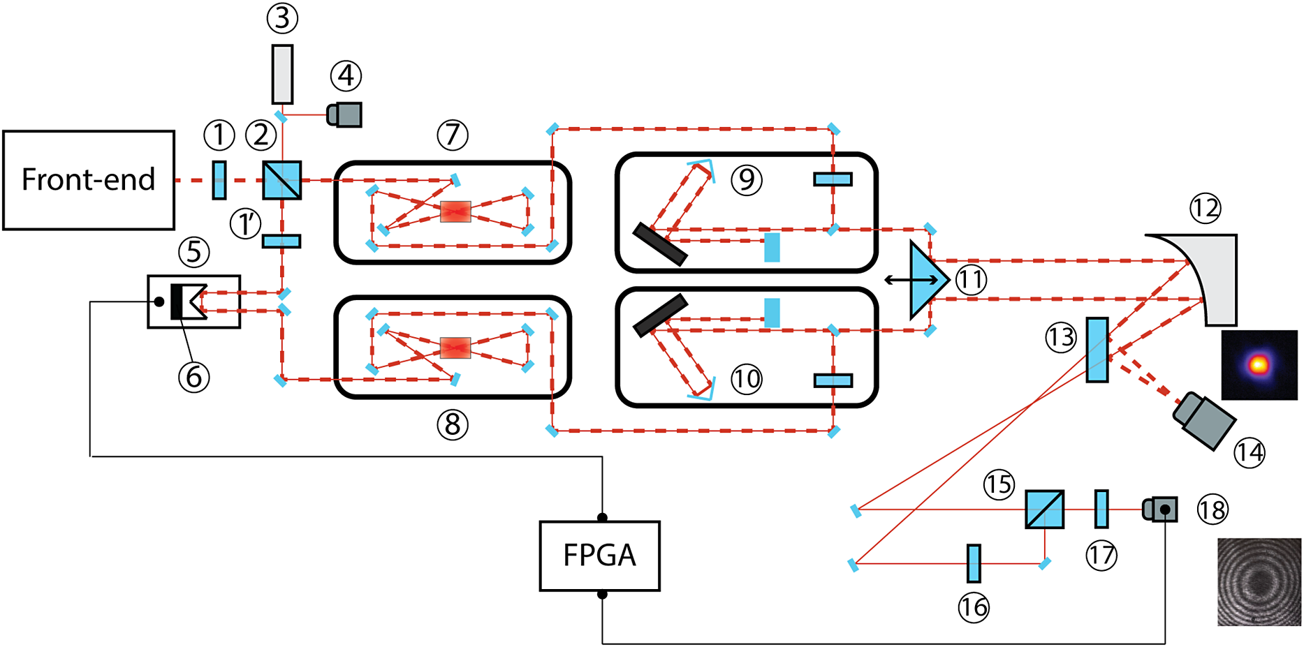
The experimental setup is presented in Figure 1. The 260 ps, 1 mJ pulse with 800 nm central wavelength generated by the front-end is divided into two replicas using a half-wave plate (1), a polarizing beamsplitter cube (2) and a second wave plate (1’) to produce the same polarization for the CWL and for the front-end laser pulses on the second arm as in the first arm. The transmitted beam replica is amplified using a two-pass amplifier (7) and compressed to approximately equal to 50 fs using a temporal compressor (9). The pulse energy after each amplifier was 2 mJ. In order to avoid burning the camera or the photodiodes, the energy was attenuated, reaching from 150 μJ to 1 mJ at the compressors’ entrance. The reflected replica is propagated through the delay line (5) and retroreflector (6), which is fixed to a fast piezoelectric actuator. This replica passes through the parallel two-pass amplifier (8) and compressor (10) to achieve also approximately equal to 50 fs pulse duration. The two parallel amplified and compressed pulses along with the co-propagated CWL are reflected by the right-angle prism (11) towards the off-axis parabolic mirror (12). The two overlapping focused ultrashort pulses are monitored by the complementary metal–oxide–semiconductor (CMOS) image sensor (14) in the focal plane. There, a fringe interference pattern is observed when the pulses are overlapped in space and time, simultaneously. A fringe tracking algorithm using the find_peaks function from the SciPy Python library was used to indicate the fringe shift for each captured image of the combined pulses. Each shift of one full fringe corresponds to a de-phasing of 2
$\pi$
 , or 2.667 fs temporal delay at the 800 nm central wavelength of the laser.
Experimental setup for coherent combination of ultrashort pulses using a dual arm 50 fs-laser system and a CWL. (1), (1’), half-wave plates; (2), polarizing beamsplitter cube; (3), long coherence length CWL with linear polarization; (4), fast photodiode; (5), linearly motorized translation stage; (6), retroreflector; (7), (8), two-pass amplifier; (9), (10), temporal pulse compressor; (11), right-angle prism; (12), off-axis parabolic mirror; (13), 90:10 (R:T) non-polarizing beamsplitter plate; (14), CMOS sensor and image of the combined pulses on it; (15), 50:50 beamsplitter cube; (16), half-wave plate; (17), quarter-wave plate; (18), Hänsch–Couillaud detector and the fringe image recorded with a camera at the detector plane.

Figure 1 Long description
A technical schematic layout of an optical experiment.
* Left side: A Front-end source emits a red dashed beam through a half-wave plate (1) into a polarizing beamsplitter cube (2). A C W L (3) and fast photodiode (4) are positioned above this junction. Below, a motorized translation stage (5) contains a retroreflector (6) for path length adjustment.
* Center section: The beam splits into two parallel arms. The top arm passes through a two-pass amplifier (7) and a temporal pulse compressor (9). The bottom arm passes through an identical two-pass amplifier (8) and compressor (10). Both arms use a series of mirrors to fold the beam path within black rectangular enclosures.
* Right side: The two beams converge at a right-angle prism (11) and are directed toward an off-axis parabolic mirror (12). The reflected light passes through a 90:10 non-polarizing beamsplitter plate (13).
* Detection: The transmitted portion reaches a C M O S sensor (14), which displays a circular heat-map image of the combined pulses. The reflected portion is directed through a 50:50 beamsplitter cube (15), a half-wave plate (16), and a quarter-wave plate (17) into a Hänsch–Couillaud detector (18). This detector shows a circular fringe interference pattern.
* Feedback Loop: An F P G A unit at the bottom center is electronically connected to the Hänsch–Couillaud detector (18) and the motorized translation stage (5) to maintain coherence.
A long coherence length diode-based CWL, with central wavelength of 798 nm and power of a few tens of mW (Cheetah, Sacher Lasertechnik) (3) is injected through the polarizing beamsplitter cube (2), and co-propagated with the pulses. The intensity of the CWL is recorded by a photodiode (4). The CWL beam (3) propagates further through the 90:10 (R:T) non-polarizing beamsplitter plate (13) towards the jitter diagnostics region comprising a 50:50 beamsplitter cube (15), a half-wave plate (16) rotating the polarization with 90° and a quarter-wave plate (17). The resulting beam is elliptically polarized, with the ellipticity encoding the relative phase delay acquired by the two beams[ Reference Hansch and Couillaud22]. Note that the energy of photons from the CWL that overlaps temporally with the 45 fs pulses is very small (more than 12 orders of magnitude), so optical interference between pulses and the CWL is negligible.
The interference pattern generated by the long coherence length laser (3) reaches the Hänsch–Couillaud detector (HCd; SmartDetect HC, LaCoSys) (18), providing, together with the CWL intensity measured with the photodiode (4), the necessary information related to the OPLD between the two amplification arms. The additional signal generated at 10 Hz repetition rate by the ultrashort pulses on the HCd is removed by electronic signal gating to avoid any potential errors in the quadrature monitoring induced by the spurious presence of the pulses on the HCd. The phase retrieval is computed only outside the interval when the short pulse is coming. The gating window was 500 μs, and we do not observe significant fluctuations when comparing the phase before and after the gating, as expected for such short times.
A field-programmable gate array (FPGA) (Moku:Pro, Liquid Instruments) is used to extract the phase value by processing the signals and computing the arctangent of their ratio. The result is used as input in a proportional–integral–derivative (PID) loop implemented in the same FPGA. The output of the PID loop is sent to a slow- (5) and a fast-acting optical delay line in one arm of the interferometer for active cancellation of disturbances. The actuator has the first resonance slightly above 1 kHz, limiting the fluctuation frequency compensation to the region below 200 Hz[ Reference Franklin, Powell and Emami-Naeini28].
3 Results and discussion
The CC results in stable interference fringe patterns in the combining volume. This generates, as a consequence, local intensity enhancement on the fringes, up to a factor of four in theory, when compared with the intensity of only one wave. The intensity enhancement and fringe contrast do not unequivocally demonstrate the CC. The field enhancement can be observed also when the relative phase of the waves varies in value by more than 1 rad in the case of long pulses (i.e., more than 10 cycles). Similarly, the visibility of the fringes does not imply CC control at the sub-1 rad level. Hence, while we did observe fringe intensity enhancement of 2.9 and a fringe visibility contrast of 0.55, we concentrated our study on the analysis of fringe stability, corresponding to the coherence of the waves. The significance of the phase control for applications is discussed in Section 3.6, where several predictions and experimental proposals that require phase control are indicated.
3.1 Ultrashort pulse fringes
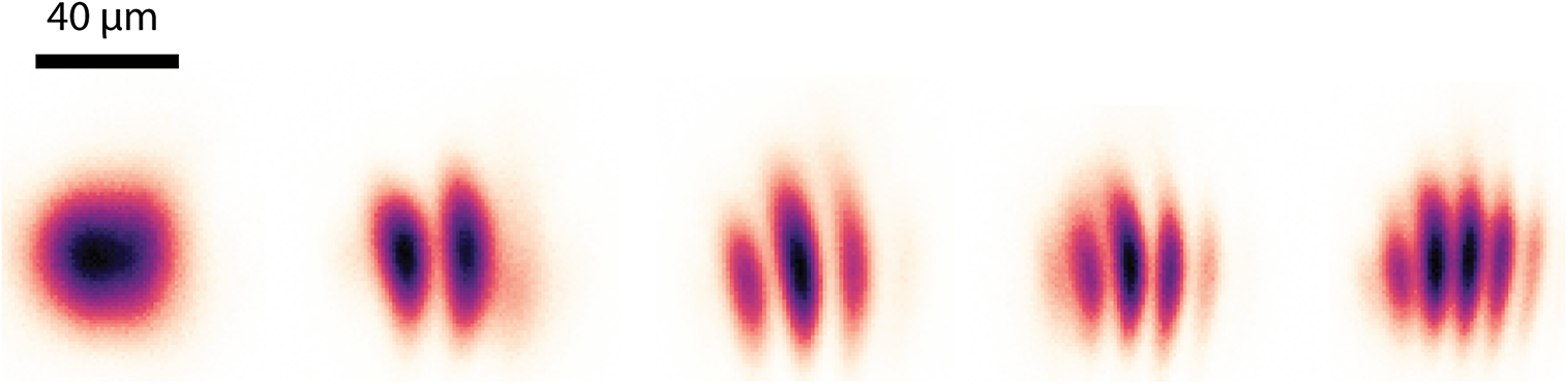
The fringes from the combined pulses are depicted in Figure 2. The inter-fringe distance
$\Delta x$
 is given by the following formula:

Fringes from the overlapped pulses in space and time in the focus of the parabola, recorded using a microscope, for angles from 2° to 10° between their propagation directions.

Figure 2 Long description
A horizontal sequence of five micrographs against a white background. A scale bar in the top left corner indicates 40 mu m.
* The first panel on the left shows a single, circular Gaussian-like spot with a dark purple core fading to orange and red at the edges.
* The second panel shows the spot splitting into two distinct vertical lobes or fringes.
* The third panel shows three vertical fringes, with the central fringe being the most intense.
* The fourth panel shows four vertical fringes.
* The fifth panel on the far right shows five distinct vertical fringes.
Across the sequence, the overall width of the pulse envelope remains relatively constant while the spatial frequency of the internal vertical interference fringes increases, resulting in more closely spaced bands.
where
$\lambda$
 is the laser wavelength and
$\theta$
is the laser wavelength and
$\theta$
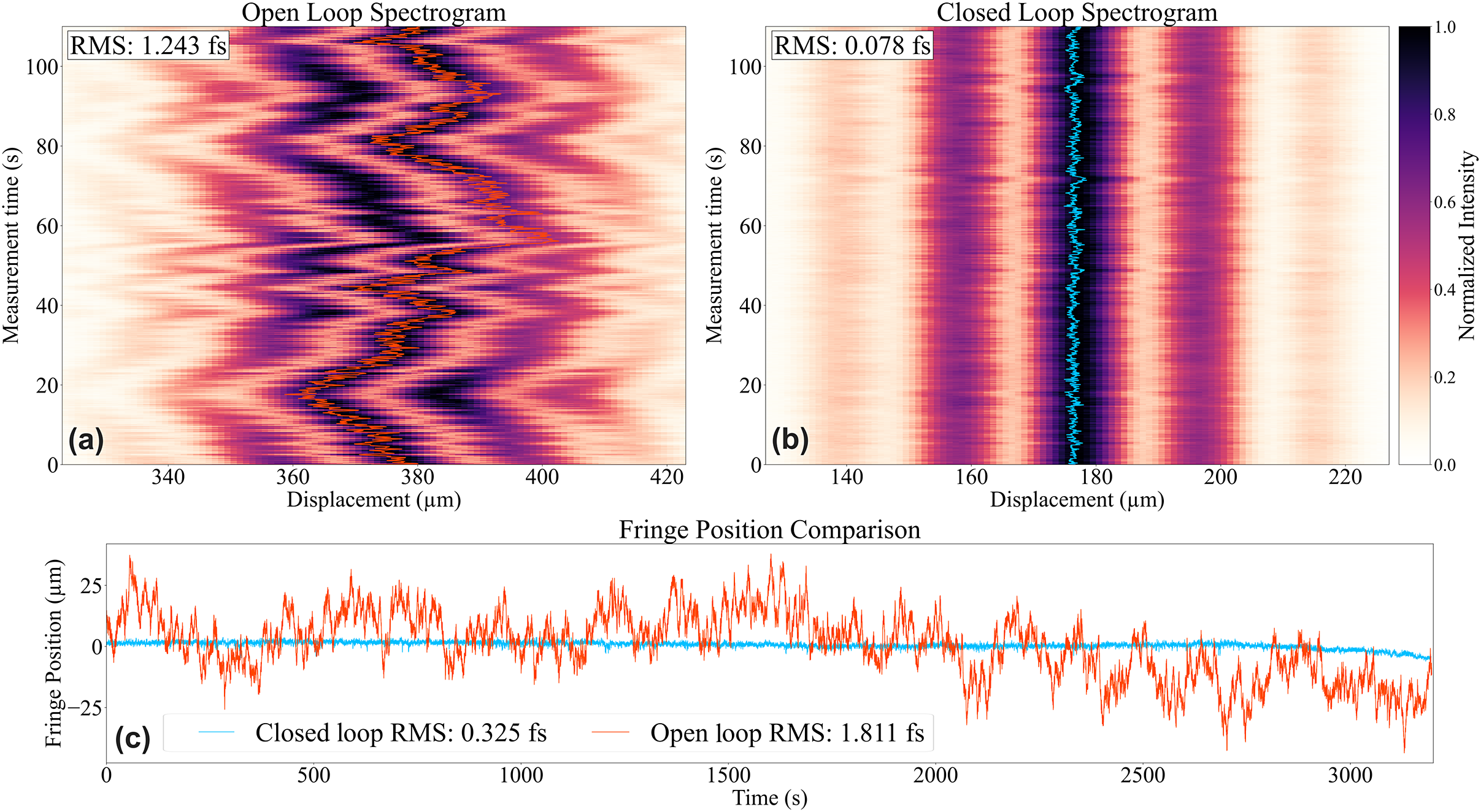
 is the angle between the two beam propagation directions. The angle between the two pulses in the focus of the parabola was varied, from 2° to approximately 10°, by moving the prism (11) in Figure 1. Note that the inter-fringe distance depends only on the angle of the beams to the focal point, and only the position of the fringes is impacted by the feedback loop state. In order to track the displacement of the fringes, an interference pattern with four visible fringes was selected, from the several shown in Figure 2. Measurements of the fringe positions for consecutive shots were made. A horizontal plot profile was obtained for each recorded image at 10 Hz, at a given pixel position of the image sensor. The resulting synthetic image is shown in Figure 3.
Interferograms from the pulses, in focus, measured with an (a) open and (b) closed loop, recorded at 10 Hz. The initial central fringe is tracked, as indicated through the continuous red and blue lines. (c) The central fringe position for 45-minute measurement, for the open loop (red) and for the closed loop (blue). One inter-fringe distance is 20 μm, corresponding to 2.67 fs of delay.

Figure 3 Long description
Panel a, titled Open Loop Spectrogram, is a heatmap with Measurement time in seconds on the y-axis from 0 to 100 and Displacement in micrometers on the x-axis from 340 to 420. The intensity fringes show a high-amplitude zigzag pattern, indicating significant drift. A red line tracks the central fringe. An R M S value of 1.243 f s is noted.
Panel b, titled Closed Loop Spectrogram, uses the same axes but with a displacement range of 140 to 220 micrometers. The intensity fringes are straight vertical bands, indicating high stability. A blue line tracks the central fringe. An R M S value of 0.078 f s is noted. A color bar to the right indicates Normalized Intensity from 0.0 to 1.0.
Panel c, titled Fringe Position Comparison, is a line graph with Time in seconds on the x-axis from 0 to 3000 and Fringe Position in micrometers on the y-axis from negative 25 to 25. The open loop data, shown as an orange line, exhibits large oscillations across the entire range with an R M S of 1.811 f s. The closed loop data, shown as a light blue line, remains nearly flat at the zero position with an R M S of 0.325 f s.
3.2 Fringe stability estimates
The temporal evolution of the fringes in open- and closed-loop operation is illustrated in the synthetic images, interferograms with one spatial and one temporal variation axis, in Figure 3. Along the spatial axis, the inter-fringe distance is 20 μm, corresponding to 2.67 fs of delay. They are measured over a 100 s time interval at 10 Hz, corresponding to 1000 consecutive shots. The relative delay for the depicted sets fluctuates with 1.243 and 0.078 fs rms, respectively. These values are already smaller than one period of the Fourier-limited pulse duration, which is 2.67 fs. The closed-loop relative delay variation for the depicted data in Figure 3(b) corresponds to
$\lambda /34$
 . The excellent stability of the setup, even in the open loop, is a consequence of its compactness, of the environment stability in the laboratory at time scales of the order of a few minutes and of the rather small length of the two arms, which is 5 m from the beamsplitter to the focus of the parabolic mirror. The evolution of the fringe position over a 45-minute interval is depicted in the lower graph in Figure 3. The corresponding long-term temporal fluctuations are 0.325 and 1.811 fs rms, respectively, indicating a spatial overlap fluctuation still better than
$\lambda /8$
. The excellent stability of the setup, even in the open loop, is a consequence of its compactness, of the environment stability in the laboratory at time scales of the order of a few minutes and of the rather small length of the two arms, which is 5 m from the beamsplitter to the focus of the parabolic mirror. The evolution of the fringe position over a 45-minute interval is depicted in the lower graph in Figure 3. The corresponding long-term temporal fluctuations are 0.325 and 1.811 fs rms, respectively, indicating a spatial overlap fluctuation still better than
$\lambda /8$
 rms in the case of closed-loop operation.
It is important to note the influence of the pointing stability on the OPLD. The two parallel propagation arms up to the focus are each about 5 m. For an initial pointing fluctuation of 5 μrad, the optical path length changes with 0.063 nm for one arm, generating, in the worst-case scenario, an OPLD of 0.126 nm. Therefore, the optical path fluctuation introduced through pointing is negligible, but it can become an issue for longer propagation paths.
The drift of the fringe position in the closed-loop operation, which was measured and is depicted in Figure 3(c), is attributed to the 1/f electronic noise in the photodiodes from the CWL feedback loop. As the OPLD-associated signal of interest detected by the photodiodes in the HCd has also very low-frequency components, it cannot be separated from the 1/f electronic noise. Hence, the corresponding amplitude of the power spectral density (PSD) of the noise introduced in the CWL feedback loop is large. This corresponds to a drift of the signal over a long observation time, as the loop tries to compensate the false signal associated with the low-frequency noise of the photodiodes in the loop.
We checked that the integrated CWL feedback loop noise is less than 8 nm for the integration interval from 10 kHz down to 10 Hz, the relevant acoustic range. This corresponds to a phase shift of 63 mrad, much less than one cycle, indicating that cycle slippage is very unlikely to occur.
3.3 Statistical analysis of the fringe stability
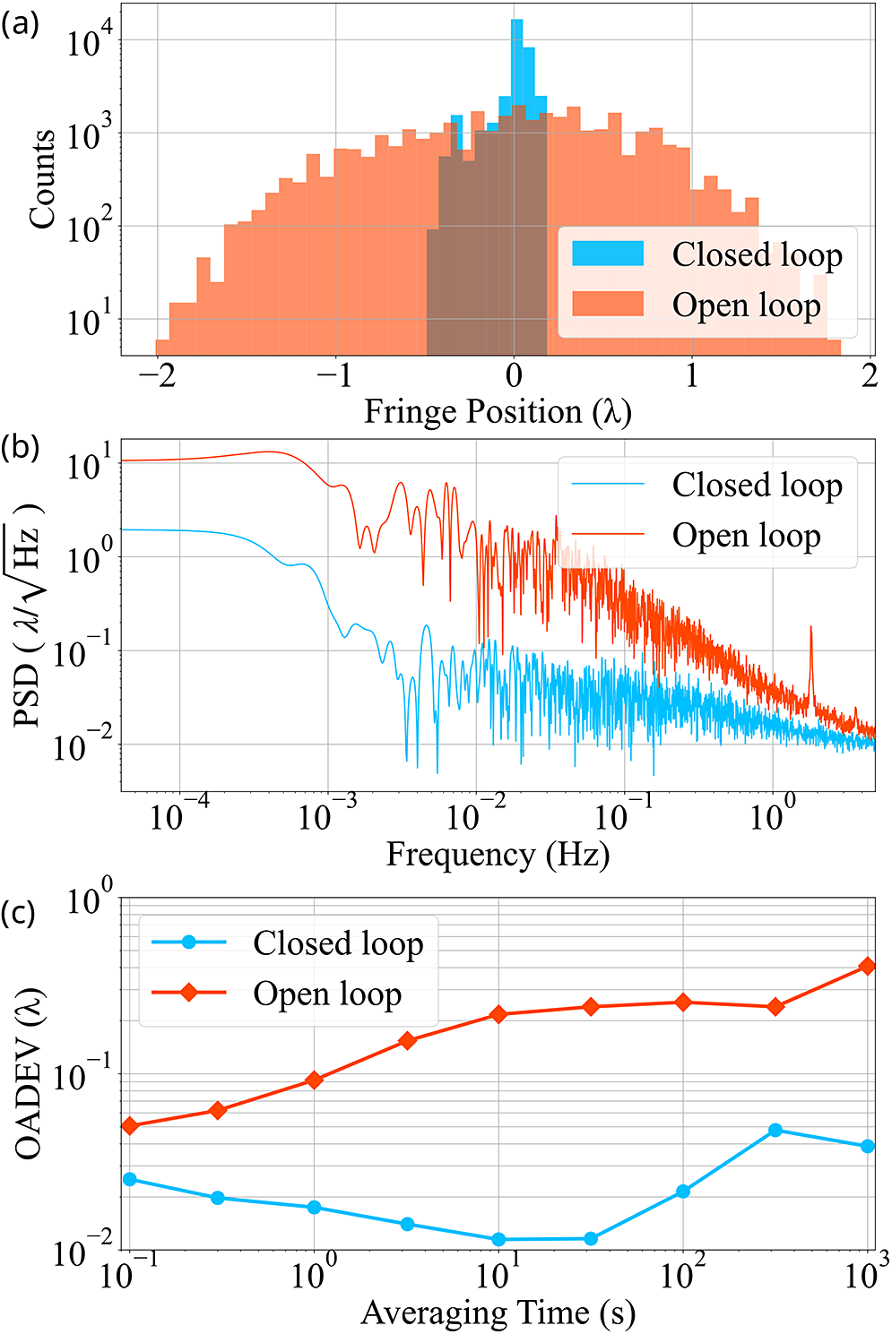
The fluctuations of the relative delay are characterized using the data extracted from the interferogram, indicated in Figure 3, lower view-graph, for both open and closed-loop operations. The histogram of the two data sets is depicted in Figure 4(a), using a logarithmic vertical scale. The peak-to-peak variation of the relative delay in the open loop is approximately equal to
$4\lambda$
 , while in the closed-loop operation it is
$0.7\lambda$
, while in the closed-loop operation it is
$0.7\lambda$
 . This rather large spread of peak-to-peak values for the closed-loop case is mostly generated by the drift observed in the last 10 minutes of the measurement.
Stability analysis of the recorded fringe position of the pulses in the focus, measured in wavelength units, for 45 minutes at 10 Hz, for open loop (red) versus closed-loop (blue) operation: (a) histogram of the fringe positions; (b) power spectral density of the fringe positions; (c) overlapping Allan deviation of the fringe position.

Figure 4 Long description
Panel a is a histogram with the x-axis showing Fringe Position in lambda units from minus 2 to 2 and the y-axis showing Counts on a logarithmic scale from 10 super 1 to 10 super 4. The open loop data in orange forms a broad, flat distribution across the entire range. The closed loop data in light blue shows a sharp, narrow peak centered at 0 lambda, indicating significantly higher stability.
Panel b is a P S D line graph with the x-axis showing Frequency in H z from 10 super minus 4 to 10 super 0 and the y-axis showing P S D in lambda over square root H z from 10 super minus 2 to 10 super 1. The red open loop line remains high, between 10 super 0 and 10 super 1, with significant noise across all frequencies. The blue closed loop line is consistently lower by one to two orders of magnitude, dropping sharply after 10 super minus 3 H z.
Panel c is an O A D E V line graph with the x-axis showing Averaging Time in seconds from 10 super minus 1 to 10 super 3 and the y-axis showing O A D E V in lambda from 10 super minus 2 to 10 super 0. The red open loop curve with diamond markers shows a steady linear increase from 0.05 to 0.4 lambda. The blue closed loop curve with circular markers shows a downward trend, reaching a minimum near 10 super 1 seconds before a slight rise, maintaining values between 0.01 and 0.05 lambda.
The performance of the control loop is shown in the PSD analysis in Figure 4(b). Closed-loop operation reduces the fluctuations of the relative delay by about one order of magnitude for low frequencies up to 10
${}^{-1}$
 Hz. Two tones at 3 Hz and at 6 Hz, observed in the open loop, are successfully suppressed in closed-loop operation, indicating a noise suppression of one order of magnitude at 3 Hz. The position of the interference pattern of the pulses, corresponding to the OPLD, reads, with 10 Hz sampling rate, the residual noise above this frequency in the stabilized CWL loop. Aliasing effects may occur; therefore, Figure 4(b) cannot be used to directly assess the CWL feedback loop performance.
We calculate the overlapping Allan deviation (OADEV) for observation time intervals from 100 ms to 1000 s[
Reference Allan29], for both the open and closed loops, as illustrated in Figure 4(c). The stability of the loop reached below
$\lambda /50$
 for time intervals between 3 and 100 s for the investigated data set.
The high stability and control of the fringes through indirect stabilization using the CWL indicate that most of the noise is generated by acoustic noise with frequencies below 200 Hz, corresponding to the feedback loop compensation capability. This observation is in line with that in Ref. [Reference Yoon, Yoon, Kim, Kim, Choi, Choi, Sung, Sung, Lee, Lee, Lee, Lee, Nam, Nam and Nam30], where the intensity fluctuation in the focus of an ultrashort and ultraintense pulse is attributed to air turbulence in the laser beam path and beam pointing. Similar challenges in noise reduction were reported for pointing stabilization and improved wavefront control at the APOLLON laser system[ Reference Ohland, Lebas, Deo, Guyon, Mathieu, Audebert and Papadopoulos31], where good focus quality was obtained after suppression of the perturbations in the frequency range below 100 Hz.
3.4 Relative phase control of the two pulses
One major feature in CC of ultrashort laser pulses is the capability to adjust the phase difference between the two pulses. This has as a consequence the shifting of the interference fringes in the focal plane.
This relative phase shifting of the laser pulses was achieved indirectly with the use of the feedback loop based on the CWL. The FPGA module can offset the loop set-point with arbitrary values, corresponding to various OPLDs.
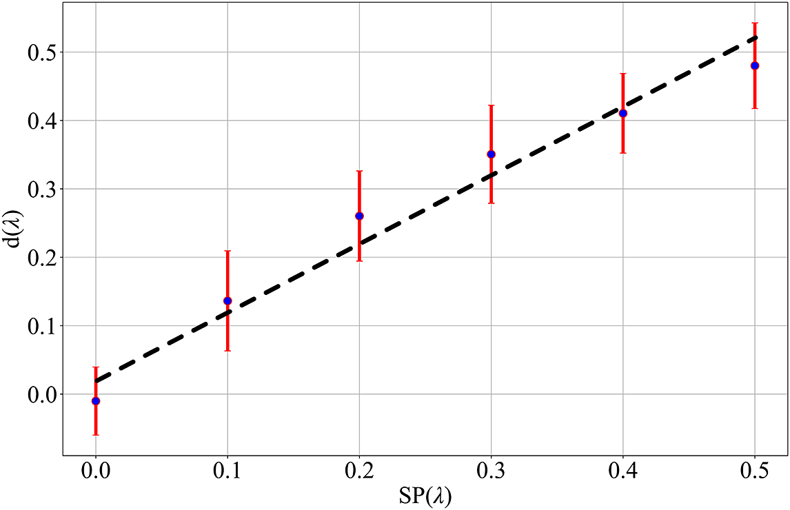
The impact of changing the CWL phase set-point from the FPGA controller on the phase shift between the laser pulses was investigated. CWL phase shifts in steps of
$\lambda /10$
 were introduced and the corresponding fringes shift of the pulses was measured for 1 minute to obtain the statistical spread for about 600 consecutive shots. The results are depicted in Figure 5, where the fringe displacement for the pulses in the focus is presented as a function of the applied offset. The rms statistical fluctuations of the fringe position are indicated in the form of error bars.
Shift of the fringes,
$d$
 , by changing the set-point SP in steps of
$\lambda /10$
, by changing the set-point SP in steps of
$\lambda /10$
 : the rms spreads of the fringe positions for each step of phase shift are represented as error bars. The dotted line represents a guide to the eye for the expected fringe position.

Figure 5 Long description
The line graph uses a Cartesian coordinate system with a grid. The horizontal X-axis is labeled S P lambda and ranges from 0.0 to 0.5 in increments of 0.1. The vertical Y-axis is labeled d lambda and ranges from 0.0 to 0.5 in increments of 0.1.
Data features include:
* A dashed black line representing the expected fringe position, showing a positive linear increase from approximately 0.02 on the Y-axis at X equals 0.0, to approximately 0.52 on the Y-axis at X equals 0.5.
* Six data points are plotted as blue dots at S P intervals of 0.1.
* Each blue dot is centered within a vertical red error bar representing the r m s spread.
* The data points closely follow the dashed line. At S P equals 0.0, the value is slightly below 0.0. At S P equals 0.1, the value is approximately 0.14. At S P equals 0.2, the value is approximately 0.26. At S P equals 0.3, the value is approximately 0.35. At S P equals 0.4, the value is approximately 0.41. At S P equals 0.5, the value is approximately 0.48.
3.5 Benchmarking the synchronization of the pulses using the liquid sheet approach
While the CC of the pulses demonstrated here indicates their precise and stable overlap, occasionally it is required to set delays between them that are significantly larger than their pulse duration. This hinders the observation of the interference fringes. In this case, the method proposed in Ref. [Reference Nazîru, Popa, Lupu, Matei, Dumitru, Nistor, Toma, Văsescu, Dăncuş, Stan and Ursescu14] can be used to monitor the delay between the pulses and define an initial zero delay within a range of picoseconds. The method is based on the stretching of one pulse to about 1 ps, in such a way that various spectral components are spread in time. The pulse is passed through a transparent material and its spectrum is measured with a spectrometer. The second pulse is kept short and it is used to switch the reflectivity of the transparent material. This produces a signature in the recorded spectrum of the first pulse, in the form of a spectral cutoff. This corresponds to the temporal delay of the short pulse with respect to the long pulse.
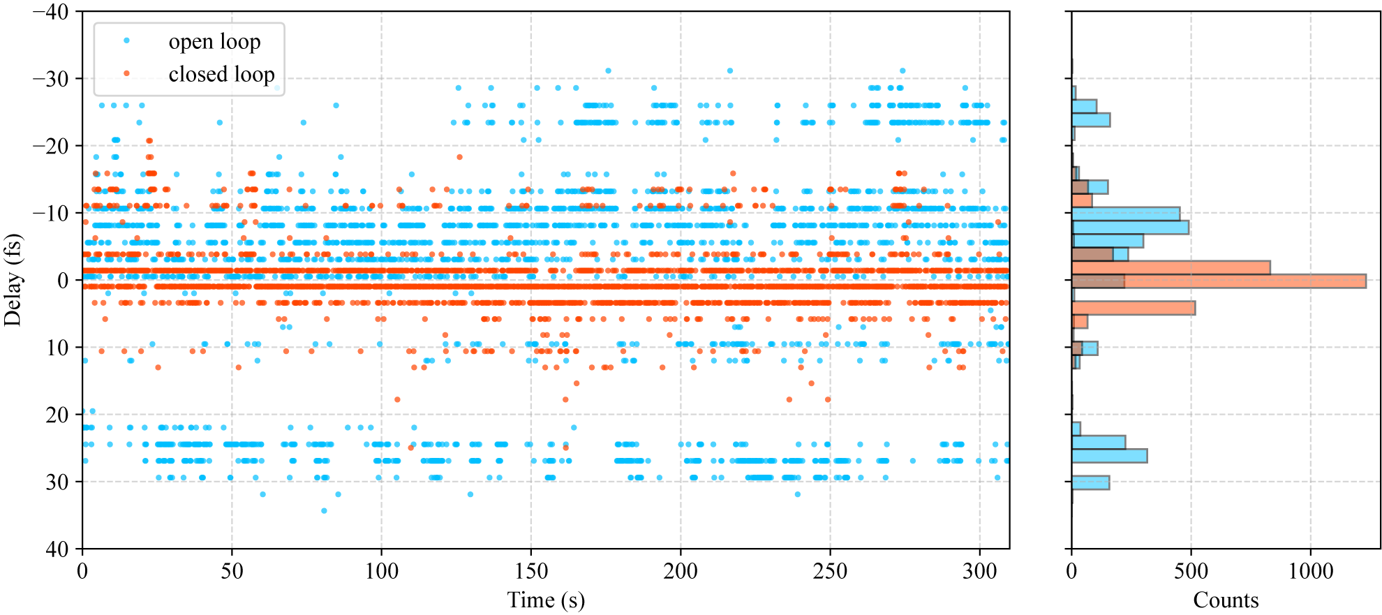
This diagnostic was employed to assess the temporal synchronization at hundreds of fs delays between the two pulses in this setup. Following the methodology described in Ref. [Reference Nazîru, Popa, Lupu, Matei, Dumitru, Nistor, Toma, Văsescu, Dăncuş, Stan and Ursescu14], the pulses were arranged in a pump–probe configuration. The probe pulse was temporally stretched to 1.28 ps, as characterized using the PM-FROG technique detailed in Ref. [Reference Popa, Nazîru, Lupu, Matei, Dumitru, Alexe, Dăncuş, Stan and Ursescu25], while the pump pulse remained at best compression. A thin liquid film, formed by the collision of two 70 μm diameter liquid jets intersecting at 90°, was used as the substrate for plasma mirror formation, operating at a repetition rate of 10 Hz. Spectral measurements were taken in both an open-loop configuration, without OPLD compensation, and a closed-loop configuration. As illustrated in Figure 6, the open-loop setup yielded a temporal jitter of 16.7 fs rms, whereas the closed-loop configuration achieved an improved stability of 4.2 fs rms.
Temporal stability and corresponding histograms of the spectral cutoff recorded over 310 s of continuous operation at 10 Hz. Two measurements were performed, in open-loop and in closed-loop CWL operation. The histogram on the right displays the distribution of relative delays for both configurations, highlighting the improvement in synchronization stability when the loop is closed.

Figure 6 Long description
The left panel is a scatter plot with Time in seconds on the x-axis from 0 to 310 and Delay in f s on the y-axis from 40 at the bottom to minus 40 at the top. Light blue dots represent open loop data, showing a wide vertical spread between minus 30 and 30 f s with distinct horizontal bands. Orange dots represent closed loop data, which are tightly concentrated around the 0 f s baseline with significantly less jitter. The right panel is a horizontal histogram sharing the y-axis with the scatter plot. The x-axis represents Counts from 0 to 1000. Light blue bars for the open loop configuration show a broad, multi-modal distribution with peaks near minus 10 and 25 f s. Orange bars for the closed loop configuration show a sharp, narrow Gaussian-like peak centered at 0 f s, reaching over 1000 counts, indicating superior synchronization stability.
The synchronization resolution of the plasma mirror-based method is limited by the resolution of the spectrometer, the chirp of the probe pulse and the fluctuations and modulations of the spectrum. The stability evaluation was performed in the
$\pm$
 2 nm vicinity of the spectral cutoff. There, the minimum achievable temporal resolution – based on the probe’s spectral characteristics and spectrometer resolution of 0.054 nm – was determined to be 2.32 fs. The temporal resolution is observed in Figure 6, in the form of discrete levels for delay, spaced at 2.32 fs. The larger delays of the order of 25 fs, also visible in Figure 6, can be attributed to the spurious presence of spectral modulations in the cutoff region of the spectrum. Consequently, the reported 4.2 fs rms value does not reflect the true synchronization jitter, but rather the noise floor set by spectral noise and mechanical instabilities. These include oscillations of the target assembly, which were operated in air and thus subject to fluctuations caused by ambient airflow. Nevertheless, a visible improvement of approximately 74.9% in rms jitter demonstrates that the synchronization method is effective.
The two synchronization measurement approaches employed in this work, the interferometric method and the plasma mirror-assisted technique, are complementary in terms of their applicable delay ranges and resolution. The interferometric method offers high temporal resolution, making it well suited for detecting fine relative delays smaller than
$\lambda /10$
 , but in a small temporal window, limited approximately to the pulse duration, which is 45 fs in our case. In contrast, the plasma mirror-assisted approach, based on a pump–probe configuration and spectral analysis, is more appropriate for measuring larger delays, typically greater than 10 fs and extending, with the length of the chirped pulse duration into the picosecond range. In our case, the range corresponds to the chirped pulse duration of 1.28 ps, but the method can be applied also to larger temporal windows of at least 300 ps[
Reference Ungureanu, Cojocaru, Banici and Ursescu32]. However, this extended range comes at the cost of reduced temporal resolution due to spectrometer resolution, spectral broadening, noise and mechanical instabilities[
Reference Popa, Nazîru, Lupu, Matei, Dumitru, Alexe, Dăncuş, Stan and Ursescu25], and was of only 3 ps in the cited reference with 300 ps chirped pulses[
Reference Ungureanu, Cojocaru, Banici and Ursescu32]. Together, these two techniques provide a comprehensive toolset for characterizing synchronization across a wide range of time delays.
, but in a small temporal window, limited approximately to the pulse duration, which is 45 fs in our case. In contrast, the plasma mirror-assisted approach, based on a pump–probe configuration and spectral analysis, is more appropriate for measuring larger delays, typically greater than 10 fs and extending, with the length of the chirped pulse duration into the picosecond range. In our case, the range corresponds to the chirped pulse duration of 1.28 ps, but the method can be applied also to larger temporal windows of at least 300 ps[
Reference Ungureanu, Cojocaru, Banici and Ursescu32]. However, this extended range comes at the cost of reduced temporal resolution due to spectrometer resolution, spectral broadening, noise and mechanical instabilities[
Reference Popa, Nazîru, Lupu, Matei, Dumitru, Alexe, Dăncuş, Stan and Ursescu25], and was of only 3 ps in the cited reference with 300 ps chirped pulses[
Reference Ungureanu, Cojocaru, Banici and Ursescu32]. Together, these two techniques provide a comprehensive toolset for characterizing synchronization across a wide range of time delays.
3.6 Potential use of phase control
The demonstrated technology has significant scientific potential when upscaled in multiple-arm high-power laser systems. The interference pattern that can be produced by two CC pulses is essential not only in future experiments related to strong-field quantum electrodynamics (QED) but also in the interaction of intense pulses with the plasma.
At intensities exceeding at least 10
${}^{22}$
 W/cm
${}^2$
W/cm
${}^2$
 , the collision of laser pulses in vacuum or in the presence of a seed electron bunch opens a window into non-linear QED processes when a high-energy electron is present. It allows one to increase the quantum non-linearity parameter
${\chi}_\mathrm{e}$
, the collision of laser pulses in vacuum or in the presence of a seed electron bunch opens a window into non-linear QED processes when a high-energy electron is present. It allows one to increase the quantum non-linearity parameter
${\chi}_\mathrm{e}$
 while the intensity is below the Schwinger limit (
$\approx$
while the intensity is below the Schwinger limit (
$\approx$
 10
${}^{29}$
10
${}^{29}$
 W/cm
${}^2$
W/cm
${}^2$
 ). These include elusive phenomena such as elastic photon–photon scattering, vacuum birefringence and electron–positron pair production – all of which are fundamentally sensitive to the spatio-temporal structure of the electromagnetic field and, crucially, to the relative phase of the pulses.
Photon–photon scattering mediated by non-linear vacuum polarization has been proposed in geometries where three intense laser pulses interact to stimulate emission of a frequency-shifted signal in a distinct direction, a four-wave mixing process[ Reference Lundström, Brodin, Lundin, Marklund, Bingham, Collier, Mendonça and Norreys33]. Related schemes use two nearly counter-propagating pulses, in which a tightly focused high-intensity beam acts as an effective phase object that modulates the wavefront of a broader probe. Such configurations have been considered both for testing non-linear electrodynamics models such as the Born–Infeld theory and for searching for axion-like particles[ Reference Tommasini and Michinel34].
Vacuum birefringence, an unobserved but robust QED prediction, occurs when a strong electromagnetic field induces anisotropic optical properties in the vacuum. In experimental scenarios, the resulting ellipticity or polarization rotation of a probe beam depends sensibly on the polarization geometry and, when multiple pulses overlap, on their relative phase[ Reference King, Di Piazza and Keitel35, Reference Bragin, Meuren, Keitel and Di Piazza36].
Electron–positron pair production can also be triggered in the standing wave formed by two colliding, linearly polarized laser pulses. In such configurations, the local field invariants depend strongly on the relative phase and polarization of the pulses, leading to pronounced sensitivity in both the total pair yield and the spatial distribution of the produced pairs[ Reference Banerjee, Singh and Fedotov37]. This phase control has been proposed as a means to manage field depletion near focus or to diagnose the internal spatio-temporal structure of tightly focused beams.
When a nucleus or other binding potential is present near the high-field region, the effective threshold for pair production can be reduced. In this case, pair creation proceeds through the laser-assisted Bethe–Heitler process or dynamically assisted tunnelling mechanisms, and the production rate inherits the same phase dependence, even in regimes where neither the laser field nor the binding potential alone would be sufficient to generate pairs[ Reference Li, Li, Su and Grobe38].
In underdense plasma, two synchronized laser pulses can provide a finely tunable mechanism for controlled electron injection into laser-driven wakefields. Such dual-pulse configurations have been used to initiate ionization injection either through direct enhancement of the local electric field or through interference-mediated modulation of the instantaneous intensity. The resulting electron beams can display improved monoenergeticity, reduced emittance and enhanced shot-to-shot stability compared with single-pulse injection[ Reference Bourgeois, Cowley and Hooker39, Reference der Leyen, Holloway, Ma, Campbell, Aboushelbaya, Qian, Antoine, Balcazar, Cardarelli, Feng, Fitzgarrald, Hou, Kalinchenko, Latham, Maksimchuk, McKelvey, Nees, Ouatu, Paddock, Spiers, Thomas, Timmis, Krushelnick and Norreys40]. Notably, the spatial and temporal overlap of the pulses determines the precise ionization site within the plasma wave. Since this overlap depends on the relative phase between the pulses, the injection process is inherently phase-sensitive[ Reference Tomassini, De Nicola, Labate, Londrillo, Fedele, Terzani and Gizzi41].
An alternative injection control is done via the interference of two laser pulses that can seed structured electron distributions within the plasma[ Reference Hornỳ, Petržílka, Klimo and Krůs42, Reference Chen, Mašlárová, Wang, Lee, Horný and Umstadter43]. In addition, the generation of a static electron grating – characterized by peak-to-background density ratios of up to 20:1 – has been proposed using the colliding-pulse configuration[ Reference Mašlárová, Horný, Chen, Wang, Li and Umstadter44]. Such periodic modulations hold promise for applications in Raman amplification, plasma-based Bragg reflectors and photonic crystal structures.
When a relativistic electron bunch traverses the standing wave formed by two counter-propagating ultraintense laser pulses, hard X-ray photons can be emitted via non-linear Thomson or Compton scattering. In this regime, the field structure is highly nonuniform and temporally dynamic[ Reference Olofsson and Gonoskov45]. As a result, the emission spectrum, angular distribution and peak photon energy are all sensitive to the carrier-envelope phase and synchronization of the colliding pulses[ Reference Mackenroth, Di Piazza and Keitel46]. This phase-sensitivity offers a potential diagnostic handle for characterizing ultrafast laser fields or tailoring photon beams for applications in imaging and nuclear spectroscopy.
Phase-controlled ion acceleration has also been explored using colliding-pulse configurations. One such concept is the ‘plasma tweezer’, formed by two counter-propagating, circularly polarized pulses of slightly different frequencies colliding on a nanometre-scale foil[ Reference Wan, Andriyash, Pai, Hua, Zhang, Li, Wu, Nie, Mori, Lu, Malka and Joshi47]. The interference of these pulses within the target generates a beat-wave pattern – a moving standing wave whose velocity and spatial profile depend on the relative phase. By synchronizing this structure with the ion population, it is possible to achieve efficient and directional ion acceleration. Other schemes utilize a secondary pulse to enhance sheath fields in traditional target-normal sheath acceleration (TNSA), again with the pulse synchronization and phase delay playing a critical role in optimizing ion yield and energy[ Reference Ferri, Siminos and Fülöp48].
At lower intensities (10
${}^{14}$
 W/cm
${}^2$
W/cm
${}^2$
 ), phase-controlled pulse collisions have been employed in gas media for high-harmonic generation (HHG). In such setups, two few-cycle laser pulses intersect at a small angle, and the emitted harmonic spectrum exhibits strong sensitivity to both the temporal delay and the optical phase difference between the pulses. This sensitivity allows one to reconstruct ultrafast dynamics and to selectively enhance or suppress harmonic orders, thus offering a route to compact attosecond pulse generation[
Reference Granados, Hsiao, Ciappina and Karki49].
), phase-controlled pulse collisions have been employed in gas media for high-harmonic generation (HHG). In such setups, two few-cycle laser pulses intersect at a small angle, and the emitted harmonic spectrum exhibits strong sensitivity to both the temporal delay and the optical phase difference between the pulses. This sensitivity allows one to reconstruct ultrafast dynamics and to selectively enhance or suppress harmonic orders, thus offering a route to compact attosecond pulse generation[
Reference Granados, Hsiao, Ciappina and Karki49].
4 Conclusion
The present work demonstrated the CC of two pulses in two parallel CPA laser arms with common front-end and separate compressors, at low repetition rate. The achieved accuracy varied from
$\lambda /8$
 rms at long time scales of the order of 45 minutes, to
$\lambda /34$
rms at long time scales of the order of 45 minutes, to
$\lambda /34$
 rms for 100 s measurements. Extensive characterization of the noise sources was provided. The advanced FPGA electronics used made possible the control of the relative phase of the pulses in non-collinear CC focus geometry in
$\lambda /10$
rms for 100 s measurements. Extensive characterization of the noise sources was provided. The advanced FPGA electronics used made possible the control of the relative phase of the pulses in non-collinear CC focus geometry in
$\lambda /10$
 steps.
For direct monitoring of delays larger than the coherence length of the pulses, the PM-FROG precision was characterized, as a first application. It was found that its intrinsic noise of the measurement is of the order of 4 fs, but it can cover delay ranges much larger than the coherence length of the pulses, as required by some experiments.
The interaction of multiple ultraintense laser pulses in a well-controlled geometry opens a novel frontier in strong-field physics and advanced particle acceleration. In particular, finely synchronized crossing laser pulses – those with sub-cycle control over relative phase and precise spatial overlap – enable field configurations that are inaccessible with single-pulse systems. These setups shall facilitate both diagnostic and functional applications across plasma physics, QED and ultrafast optics, opening a direct[ Reference Lebegue, Froidevaux, Ohland, Rapeneau, Badarau, de Sousa, Meignien, Doudet, Chan, Wattellier, Audebert, Papadopoulos and Druon21] or indirect[ Reference Chen, Xu, Yu, Cao, Chen, Bi, Jiang, Zhao, Hu, Yu and Zou50] gateway to extreme-field phenomena.
Author contributions
Conceptualization, D.U.; methodology, A.N., S.P., D.G.M., D.U.; software, A.D., D.G.M.; validation, A.N., S.P.; formal analysis, A.N., A.D., S.P., D.G.M., D.U.; investigation, A.N., S.P., A.D., D.G.M., V.A.P., A.H.O., D.C., C.D., O.C., R.D., B.S., L.V., S.R., A.G., V.H., P.T., D.U.; resources, M.G., I.D., D.U.; data curation, S.P., A.N., A.D.; writing – original draft preparation, A.N., S.P., D.G.M., A.D., V.H., P.T., D.U.; writing – review and editing, A.N., S.P., D.G.M., A.D., V.H., P.T., D.U.; visualization, A.N., S.P., D.G.M., A.D., D.U.; supervision, D.U.; project administration, D.U.; funding acquisition, I.D., D.U. All authors have read and agreed to the published version of the manuscript.
Acknowledgements
The authors are grateful to Dr. Claudiu Stan for providing the liquid target associated equipment and for useful discussions, and to Daniel Popa, Adrian Toader and Nicu Stan for logistic support. The operation of ELI-NP is financed by the Romanian Ministry for Research, Innovation and Digitalization through the ELI-NP IOSIN programme and the Nucleu programme PN 23 21 01 05. This work was supported by ELI-RO/2023/LASCOMB, funded by the Institute of Atomic Physics, Romania. S.P., A.D., A.H.O. and D.U. acknowledge support from ELI-RO/DFG/2025_013 IATP-NP 2.0, funded by the Institute of Atomic Physics, Romania. The building of ELI-NP was funded by the Romanian Government and the European Union through the European Regional Development Fund and the Competitiveness Operational Programme (1/07.07.2016, COP, ID 1334), as part of the Extreme Light Infrastructure – Nuclear Physics (ELI-NP) Phase II project.



 Open access

