





1. Introduction
The wavemaker problem consists of waves launched from a boundary into a medium at rest. It is a fundamental problem for inviscid flows with physical applications, including surface waves in reservoirs or lakes produced by the movement of a solid body (Chwang Reference Chwang1983b). In the laboratory, wavemakers provide the means to generate finite-amplitude water waves (Chwang Reference Chwang1983a). Some examples highlighting the rich variety of nonlinear wave dynamics that is possible include the generation of cnoidal waves (Goring & Raichlen Reference Goring and Raichlen1980), interacting undular bores (Trillo et al. Reference Trillo, Deng, Biondini, Klein, Clauss, Chabchoub and Onorato2016) and evidence of a soliton gas (Redor et al. Reference Redor, Barthélemy, Michallet, Onorato and Mordant2019) from the fission of a sinusoidal wave and the controlled generation of an isolated rogue wave (Chabchoub, Hoffmann & Akhmediev Reference Chabchoub, Hoffmann and Akhmediev2011; Tikan et al. Reference Tikan2022).
This paper presents an alternative fluid medium, called a conduit, in which to investigate the wavemaker problem in the linear and nonlinear regimes. The pressure-driven, buoyant, core–annular flow between two miscible Stokes fluids with a small core-to-annular fluid viscosity ratio is a simple, conducive laboratory setting for the quantitative experimental study of nonlinear wave propagation (Olson & Christensen Reference Olson and Christensen1986; Scott, Stevenson & Whitehead Reference Scott, Stevenson and Whitehead1986; Helfrich & Whitehead Reference Helfrich and Whitehead1990; Maiden et al. Reference Maiden, Lowman, Anderson, Schubert and Hoefer2016, Reference Maiden, Franco, Webb, El and Hoefer2020). This setting is quite different from more traditional core–annular flows, such as oil–water, subject to non-negligible inertial and surface tension effects resulting in a variety of instabilities (Joseph et al. Reference Joseph, Bai, Chen and Renardy1997). Instead, we operate in a vanishing Reynolds number regime where the flow is convectively unstable (d'Olce et al. Reference d'Olce, Martin, Rakotomalala, Salin and Talon2009) and can be effectively interpreted as a deformable, fluid-filled pipe (Olson & Christensen Reference Olson and Christensen1986; Lowman & Hoefer Reference Lowman and Hoefer2013) due to very slow mass diffusion across the conduit interface (Maiden et al. Reference Maiden, Lowman, Anderson, Schubert and Hoefer2016). Conduits model viscously deformable media in a variety of physical environments such as magma in the Earth's mantle (Whitehead & Helfrich Reference Whitehead and Helfrich1990) and channelized water flow under glaciers (Stubblefield, Spiegelman & Creyts Reference Stubblefield, Spiegelman and Creyts2020). A schematic of the flow configuration is shown in figure 1.
Schematic of the core–annular flow configuration. The interior fluid rises buoyantly within the exterior fluid with densities  $\rho ^{(i)}<\rho ^{(e)}$ and viscosities $\mu ^{(i)}\ll \mu ^{(e)}$, respectively. The vertical volumetric flow rate is $Q(z,t)$, the cross-sectional area of the interface is $A(z,t)$ and $A_0$ is the background, mean area of the conduit.

In traditional pressure-driven core–annular flows, finite-amplitude dynamics can be studied in the long-wavelength regime using an approximate interfacial wave model consisting of nonlinear advective and dissipative terms such as those asymptotically derived in Camassa & Ogrosky (Reference Camassa and Ogrosky2015). These models can be viewed as generalizations of the famous Kuramoto–Sivashinsky equation (Sivashinsky Reference Sivashinsky1977; Kuramoto Reference Kuramoto1978), which exhibits spatio-temporal chaos. In contrast, the viscous core–annular flow of a pressure-driven Stokes core fluid within an annulus of another, miscible, heavier Stokes fluid is accurately modelled by the so-called conduit equation
 \begin{equation} A_t + (A^2)_z - (A^2(A^{{-}1}A_t)_z)_z = 0, \end{equation}
for the normalized, axisymmetric cross-sectional area  $A$ of a fluid conduit at non-dimensional vertical height $z$ and time $t$. The conduit equation is an expression of mass conservation subject to buoyancy-induced nonlinear advection and nonlinear, non-local dispersion due to interfacial stresses that is obtained from the two-fluid Navier–Stokes equations in the small Reynolds number, small core-to-annular viscosity ratio and long-wavelength regime with no assumption on wave amplitude (Olson & Christensen Reference Olson and Christensen1986; Lowman & Hoefer Reference Lowman and Hoefer2013). Unlike models of traditional core–annular flows, this third-order dispersive nonlinear wave equation is more closely analogous to the Korteweg-de Vries equation of shallow water wave fame (Korteweg & de Vries Reference Korteweg and de Vries1895).
Much as in the aforementioned hydrodynamic wavemaker case, the viscous conduit is a laboratory environment for the study of a variety of nonlinear wave dynamics. Past experimental studies include solitary waves (Olson & Christensen Reference Olson and Christensen1986; Scott et al. Reference Scott, Stevenson and Whitehead1986) and their interactions (Helfrich & Whitehead Reference Helfrich and Whitehead1990; Lowman, Hoefer & El Reference Lowman, Hoefer and El2014), periodic waves (Olson & Christensen Reference Olson and Christensen1986; Kumagai & Kurita Reference Kumagai and Kurita1998), solitary wave fission (Anderson, Maiden & Hoefer Reference Anderson, Maiden and Hoefer2019; Maiden et al. Reference Maiden, Franco, Webb, El and Hoefer2020), dispersive shock waves (DSWs) (Maiden et al. Reference Maiden, Lowman, Anderson, Schubert and Hoefer2016) and interactions between solitary waves and DSWs (Maiden et al. Reference Maiden, Anderson, Franco, El and Hoefer2018). Quantitative observational agreement with the conduit equation (1.1) has been achieved in certain regimes. But such agreement has largely been confined to the long-wave, nonlinear regime. Herein, we experimentally investigate the generation of long and short periodic travelling waves in a viscous fluid conduit using a wavemaker with a view toward understanding their fundamental properties.
Periodic wavetrains have already been observed and studied in viscous fluid conduits. Some of the earliest studies generated periodic waves by either quickly increasing the injection rate from one constant value to another constant value (Scott et al. Reference Scott, Stevenson and Whitehead1986; Kumagai & Kurita Reference Kumagai and Kurita1998) or tracking the periodic waves that trail a rising diapir from a plume of injected fluid (Olson & Christensen Reference Olson and Christensen1986). However, since the injection rate was held constant after the initial change, both scenarios involve a different dynamics than we consider here. In the first case, we now understand that a step up in injection rate from a non-zero previous rate results in a DSW consisting of a slowly varying, expanding periodic travelling wave that ultimately returns to a constant injection rate, i.e. it is transient (Maiden et al. Reference Maiden, Lowman, Anderson, Schubert and Hoefer2016). In the latter case, it is likely that an oscillatory (absolute) instability (d'Olce et al. Reference d'Olce, Martin, Rakotomalala, Salin and Talon2009) developed due to sufficiently large injection rate rather than the convective instability regime in which we operate. In this work, we controllably create high-quality linear and nonlinear periodic travelling waves by use of a carefully selected time-periodic injection rate by evaluating exact periodic travelling wave solutions of the model conduit equation.
The major objective of this work is the reliable generation of both linear and nonlinear, cnoidal-type waves from a wavemaker. Laboratory measurement constrained by boundary control is realized by injecting an interior fluid of lower viscosity and lower density into a more viscous exterior fluid using a piston pump. Limitations are investigated, and the experiment is compared with the theory of the boundary value problem for the conduit equation. We find that, although the exact periodic travelling wave solutions to the conduit equation exhibit quantitative agreement with our experimental observations, a deviation in the linear dispersion relation occurs for sufficiently short waves. In order to describe the linear waves in the shorter-wavelength regime, we obtain the exact solution for two-Stokes flow linear interfacial wave propagation. Previous work by Yih (Reference Yih1963, Reference Yih1967) and Hickox (Reference Hickox1971) studied the linear instability of core–annular flows for the Navier–Stokes equations. Within a parameter regime consistent with our experimental conditions, the instability has been shown to be convective (d'Olce et al. Reference d'Olce, Martin, Rakotomalala, Salin and Talon2009; Selvam et al. Reference Selvam, Talon, Lesshafft and Meiburg2009). However, none of these works obtained an analytical solution to the problem, instead relying upon numerical solutions. Herein, we develop a model for recirculating viscous core–annular flows in our experiments and obtain the exact solution to the Stokes equations for azimuthally symmetric, small-amplitude perturbations. The two-Stokes linear dispersion relation is shown to agree with the conduit equation's linear dispersion relation in the limit of high viscosity contrast and long waves.
The paper is structured as follows. First, we provide some background material on the conduit equation and periodic travelling waves. Then we derive the exact linear dispersion relation for two-Stokes core–annular flow in § 2. Analytical results for an idealized recirculating flow with azimuthally symmetric linear interfacial waves and their asymptotic expansions are presented. Section 3 describes linear modulation theory applied to the initial-boundary value problem for both the conduit equation and two-Stokes flow. In § 4, experimental methods and analysis of linear and nonlinear periodic travelling waves in a viscous fluid conduit are provided. Finally, we conclude in § 5.
1.1. The conduit equation
The conduit equation (1.1) is an accurate partial differential equation model of conduit interfacial waves whose mathematical structure and solutions have been analysed (Harris & Clarkson Reference Harris and Clarkson2006; Simpson & Weinstein Reference Simpson and Weinstein2008; Maiden & Hoefer Reference Maiden and Hoefer2016; Johnson & Perkins Reference Johnson and Perkins2020).
The conduit equation exhibits solutions that are reminiscent of the Korteweg–de Vries (KdV) and Benjamin–Bona–Mahoney (BBM) equations, both models of shallow water waves. In fact, the conduit equation can be reduced to the BBM and KdV equations for long waves and weak nonlinearity. Let
 \begin{equation} T = \delta^{1/2}t, \quad Z= \delta^{1/2} z, \end{equation}
and
 \begin{equation} A(z,t) = 1+\delta u(Z,T) + \dots, \end{equation}
where  $\delta \ll 1$ is the small amplitude parameter and $u(Z,T)$ is the scaled, leading-order deviation in cross-sectional area. Insertion of this ansatz into (1.1) and keeping the leading and first-order terms results in the BBM equation (Benjamin, Bona & Mahony Reference Benjamin, Bona and Mahony1972)
 \begin{equation} u_T + 2u_Z + 2 \delta uu_Z - \delta u_{ZZT}= 0 . \end{equation}
Since  $u_T=-2u_Z+{O}(\delta )$ implies $u_{ZZT}=-2u_{ZZZ}+{O}(\delta )$, we obtain the KdV equation $u_T + 2u_Z + 2\delta u u_Z + 2\delta u_{ZZZ} = 0$ to the same order of accuracy (Whitehead & Helfrich Reference Whitehead and Helfrich1986). Hence, both the BBM and KdV equations are asymptotically equivalent to the conduit equation (1.1) in the weakly nonlinear, long-wavelength regime. Notably, the BBM equation (1.4) with $\delta = 1$ has the same linear dispersion relation as the conduit equation (1.1) on a unit-mean background.
The travelling wave solutions of both the BBM and KdV equations may be expressed in terms of the Jacobi cosine elliptic function cn, the so-called cnoidal wave solutions (Korteweg & de Vries Reference Korteweg and de Vries1895), as
 \begin{equation}
\left.\begin{gathered} u(Z,T) = \beta + (\gamma-\beta)
\text{cn}^2 \left[ \left( \frac{\gamma-\alpha}{6 \chi}
\right)^{1/2} (Z-cT); m \right], \\ c =
\frac{2\delta(\alpha+\beta+\gamma)}{3}+2, \quad
m=\frac{\gamma-\beta}{\gamma-\alpha} ,
\end{gathered}\right\}
\end{equation}
\begin{equation}
\left.\begin{gathered} u(Z,T) = \beta + (\gamma-\beta)
\text{cn}^2 \left[ \left( \frac{\gamma-\alpha}{6 \chi}
\right)^{1/2} (Z-cT); m \right], \\ c =
\frac{2\delta(\alpha+\beta+\gamma)}{3}+2, \quad
m=\frac{\gamma-\beta}{\gamma-\alpha} ,
\end{gathered}\right\}
\end{equation}
where  $\alpha,\beta,\gamma$ are independent, free parameters. The only difference between the KdV and BBM cnoidal solutions is in the wavenumber coefficient $\chi$: $\chi _{KdV} = 2$, $\chi _{BBM} = c$. In the limit $\beta \to \alpha$ with $\beta \neq \gamma$, (1.5) reduces to a sech $^2$ solitary wave solution and in the small-amplitude limit $0 < \gamma - \beta \ll 1$, (1.5) becomes a sinusoidal travelling wave.
1.2. The wavemaker problem and periodic travelling wave solutions
For a time-harmonic boundary condition in the linear regime, the Sommerfeld radiation condition (Sommerfeld Reference Sommerfeld1912, Reference Sommerfeld1949) can be used to select a particular solution, either a propagating wave or a spatially decaying wave, by requiring a causal solution with only outgoing waves at infinity. The cross-over between the two behaviours occurs at zero group velocity. This condition has been applied to many problems in fluid dynamics and elsewhere (see, e.g. Bühler Reference Bühler2014) and will be applied to the conduit equation.
The conduit equation (1.1) obeys the scaling invariance
 \begin{equation} A^* = \frac{A}{\bar{A}}, \quad z^*=\bar{A}^{{-}1/2}z, \quad t^* = \bar{A}^{1/2}t, \end{equation}
where  $\bar {A}>0$, which leaves (1.1) invariant. Owing to this scaling invariance, we will, without loss of generality, assume that the periodic travelling wave has unit mean. In this work, we study the wavemaker problem for a viscous fluid conduit subject to a specially chosen time-dependent, periodic input with amplitude $a$ and injection frequency $\omega _0$ at the boundary. The wavemaker initial-boundary value problem is
 \begin{equation} \left.\begin{gathered} A(z,0) = 1, \quad z \geqslant 0, \\ A(0,t) = 1+f(t), \quad t \geqslant 0,\quad f(t+T_0)=f(t), \quad t>0, \quad T_0 = \frac{2{\rm \pi}}{\omega_0}, \end{gathered}\right\} \end{equation}
where  $f(t)$ is the zero mean periodic profile with frequency $\omega _0>0$, $f(0)=f'(0)=0$, $\int _0^{T_0} f(t) \,\textrm {d}t =0$.
Conduit periodic travelling wave solutions satisfy  $A(z,t) = \phi (\theta )$, $\theta =kz-\omega t$, $\phi (\theta +2{\rm \pi} )=\phi (\theta )$ for $\theta \in \mathbb {R}$, wavenumber $k \geq 0$, and frequency $\omega \geq 0$ subject to the nonlinear ordinary differential equation (Olson & Christensen Reference Olson and Christensen1986)
 \begin{equation} -\omega \phi' + k (\phi^2)' + \omega k^2 (\phi^2 (\phi^{{-}1}\phi')')'=0. \end{equation}
Integrating (1.8) twice results in
 \begin{equation} (\phi')^2 = g(\phi) \equiv{-}\frac{2}{k^2}\phi - \frac{2}{\omega k}\phi^2\ln\phi + c_1 +c_2\phi^2, \end{equation}
where  $c_{1,2}$ are integration constants. Conduit solitary wave solutions are asymptotically stable (Simpson & Weinstein Reference Simpson and Weinstein2008) and periodic travelling waves are modulationally stable for sufficiently long wavelengths (Maiden & Hoefer Reference Maiden and Hoefer2016; Johnson & Perkins Reference Johnson and Perkins2020).
Upon linearization of (1.1) as  $A(z,t)-1 \propto \cos (k z-\omega t)$, the conduit equation exhibits a bounded dispersion relation
 \begin{equation} \omega = \frac{2k}{1+k^2} . \end{equation}
For the wavemaker problem, it is helpful to invert the linear dispersion relation (1.10) and solve for  $k(\omega )$. In order to select the correct branch, we apply the radiation condition (positive group velocity or spatial decay) to obtain
 \begin{equation}
k(\omega) = \begin{cases}
\dfrac{1-\sqrt{1-\omega^2}}{\omega}, & 0<\omega\leqslant1
\\ \dfrac{1+i\sqrt{\omega^2-1}}{\omega}, & \omega>1
\end{cases},
\end{equation}
\begin{equation}
k(\omega) = \begin{cases}
\dfrac{1-\sqrt{1-\omega^2}}{\omega}, & 0<\omega\leqslant1
\\ \dfrac{1+i\sqrt{\omega^2-1}}{\omega}, & \omega>1
\end{cases},
\end{equation}
where wavenumbers  $k$ for frequencies $0<\omega \leqslant 1$ are real, implying steady wave propagation. For $\omega >1$, $k(\omega )$ exhibits a positive imaginary part so that these waves spatially decay (equivalent to Gaster Reference Gaster1962). The frequency $\omega _{cr}=1$ is therefore the critical frequency, above which waves decay and get arrested. The corresponding critical wavenumber $k_{cr}=1$ satisfies $k_{cr}=k(\omega _{cr})$.
In the weakly nonlinear regime, we can obtain approximate periodic travelling wave solutions when the amplitude is small and the wavenumber is sufficiently far away from 0. The weakly nonlinear approximation with three harmonics takes the form
 \begin{equation} \phi(\theta; k, a) = 1 + \dfrac{a}{2} \cos(\theta) + \dfrac{1+k^2}{48k^2} a^2\cos(2\theta) + \dfrac{1+k^2}{1536k^4}a^3\cos(3\theta) + O(a^4), \end{equation}
where  $\theta =k z-\omega t$, the amplitude $0< a \ll 1$, the wavenumber $k^2 \gg a$ and the frequency $\omega$ is approximately
 \begin{equation} \omega(k,a) = \frac{2k}{1+k^2} + a^2 \frac{1-8k^2}{48k(1+k^2)} + O(a^4). \end{equation}
Alternatively, we can express the weakly nonlinear expansions in terms of  $\omega$ and obtain
 \begin{align} \phi(\theta,\omega,a) & = 1 +\frac{a}{2}\cos(\theta)+\frac{a^2}{24\left(1-\sqrt{1-\omega^2}\right)}\cos(2\theta) \nonumber\\ & \quad + \frac{\left({-}1-\sqrt{1-\omega^2}\right) a^3 }{768\left({-}2+\omega^2+2\sqrt{1-\omega^2}\right)}\cos(3\theta) + \dots, \end{align}
 \begin{align} k(\omega,a) &= \frac{1-\sqrt{1-\omega^2}}{\omega} +\frac{\left({-}9+ \dfrac{7}{\sqrt{1-\omega^2}}\right)}{96\omega} a^2 + \dots, \end{align}
for  $0 < \omega < 1$. The induced mean occurs at ${O}(a^2)$ and must be taken into account when nonlinear modulations are considered (Maiden & Hoefer Reference Maiden and Hoefer2016).
The nonlinear dispersion relation is explicitly expressed in terms of three roots  $0< u_1< u_2< u_3$ of $g(\phi )$ in (1.9) (Lowman & Hoefer Reference Lowman and Hoefer2013) and phase velocity $U$ so that
 \begin{gather} \exp U = u_1^{{u_1^2(u_2+u_3)}/{(u_3-u_1)(u_2-u_1)}} u_2^{-{u_2^2(u_3+u_1)}/{(u_3-u_2)(u_2-u_1)}} u_3^{{u_3^2(u_2+u_1)}/{(u_3-u_1)(u_3-u_2)}}. \end{gather}
The numerically computed conduit nonlinear dispersion relation  $\omega =kU$ is presented in figure 2, where the red dashed line corresponds to the edge of the existence region. The wave amplitude, wavenumber and mean are given by
 \begin{equation} a = u_3-u_2, \quad k={\rm \pi} \left( \int_{u_2}^{u_3} \frac{{\rm d}u}{\sqrt{g(u)}} \right)^{{-}1}, \quad \bar{\phi}=\frac{k}{\rm \pi} \int_{u_2}^{u_3} \frac{u \,{\rm d}u}{\sqrt{g(u)}}, \end{equation}
where  $g(u)$ is defined in equation (1.9). The limits $u_2 \to u_1$ and $u_2 \to u_3$ correspond to the solitary wave and linear, harmonic limits, respectively. These periodic travelling wave solutions are analogous to the cnoidal solutions of KdV and BBM (1.5) and therefore we will refer to them as cnoidal-like throughout this work.
Contour plot of numerically computed conduit dispersion relation  $k(\omega,a)$. Beyond the red dashed line, no real $k(\omega,a)$ is obtained.

2. Two-Stokes flow
Since the conduit equation (1.1) and its linear dispersion relation (1.10), (1.11) are derived under long wavelength assumptions, we now seek a more accurate description of linear waves by analysing the free interface between two-Stokes fluids.
2.1. Primary recirculating flow
Interfacial waves generated by the buoyant dynamics between two miscible Stokes fluids with a small viscosity ratio  $\epsilon =\mu ^{(i)}/\mu ^{(e)}$ are described by continuity equations for mass conservation and Stokes equations for momentum conservation
 $$\begin{gather} \boldsymbol{\nabla}\boldsymbol{\cdot} {\tilde{\boldsymbol{u}}}^{(i,e)} = 0, \end{gather}$$
 $$\begin{gather}-\boldsymbol{\nabla} \tilde{p}^{(i,e)} + \boldsymbol{\nabla}\boldsymbol{\cdot} \tilde{{\boldsymbol{\mathsf{\sigma}}}}^{(i,e)} = 0, \end{gather}$$
for the interior and exterior fluids, denoted by superscripts  $i$ or $e$, respectively. The velocity fields $\tilde {\boldsymbol {u}}^{(i,e)} = (\tilde {u}_{\tilde {r}}^{(i,e)}, \tilde {u}_{\tilde {z}}^{(i,e)})$ are given in cylindrical coordinates assuming azimuthal symmetry. The pressure deviation from hydrostatic is $\tilde {p}^{(i,e)}$ and the deviatoric stress tensor is $\tilde {{\boldsymbol{\mathsf{\sigma}}} }^{(i,e)}=\mu ^{(i,e)}[\boldsymbol {\nabla } \tilde {\boldsymbol {u}} + (\boldsymbol {\nabla } \tilde {\boldsymbol {u}})^\textrm {T}]$, where $\mu ^{(i,e)}$ denotes the fluid viscosity. The kinematic boundary condition between the two fluids at $\tilde {r}=\tilde {R}(z,t)$ incorporates the time dynamics
 \begin{equation} \tilde{u}_{\tilde{r}}^{(i)} = \frac{\partial \tilde{R}}{\partial \tilde{t}} + \tilde{u}_{\tilde{z}}^{(i)}\frac{\partial \tilde{R}}{\partial \tilde{z}}, \quad \tilde{r}=\tilde{R}(\tilde{z},\tilde{t}). \end{equation}
The remaining boundary conditions include the continuity of normal and tangential velocities
 \begin{equation} [\tilde{\boldsymbol{u}}\boldsymbol{\cdot} \hat{\tilde{\boldsymbol{n}}}_c]_j = [\tilde{\boldsymbol{u}} \boldsymbol{\cdot}\hat{\tilde{\boldsymbol{t}}}_c]_j =0 , \quad \tilde{r} = \tilde{R}(\tilde{z},\tilde{t}), \end{equation}
and continuity of normal and tangential stresses
 \begin{equation} [\hat{\tilde{\boldsymbol{n}}}_c \boldsymbol{\cdot} \tilde{\boldsymbol{\mathsf{T}}} \boldsymbol{\cdot}\hat{\tilde{\boldsymbol{n}}}_c]_j = [\hat{\tilde{\boldsymbol{t}}}_c \boldsymbol{\cdot} \tilde{\boldsymbol{\mathsf{T}}} \boldsymbol{\cdot} \hat{\tilde{\boldsymbol{n}}}_c]_j = 0, \quad \tilde{r} = \tilde{R}(\tilde{z},\tilde{t}), \end{equation}
where  $[]_j$ represents the difference in the exterior and interior fluid quantities, $\hat {\tilde {\boldsymbol {n}}}_c$ is the outward pointing unit normal to the interface and $\hat {\tilde {\boldsymbol {t}}}_c$ is the unit tangent to the interface. Here, $\tilde {\boldsymbol{\mathsf{T}}}^{(i,e)}=\tilde {{\boldsymbol{\mathsf{\sigma}}} }^{(i,e)} - \boldsymbol{\mathsf{I}} \tilde {p}^{(i,e)}$ is the stress tensor and $\boldsymbol{\mathsf{I}}$ denotes the identity operator. No-slip and no-penetration boundary conditions at the outer wall $\tilde {r}=\tilde {D}$ require $\tilde {u}_{\tilde {z}}^{(e)}(\tilde {D})=0$ and $\tilde {u}_{\tilde {r}}^{(e)}(\tilde {D})=0$. Boundary conditions along the symmetry axis are imposed as
 \begin{equation} \dfrac{\partial \tilde{\boldsymbol{u}}_{\tilde{z}}^{(i)}}{\partial \tilde{r}}=0, \quad \tilde{\boldsymbol{u}}_{\tilde{r}}^{(i)}=0, \quad \dfrac{\partial \tilde{p}^{(i)}}{\partial \tilde{r}}=0, \quad \text{at } \tilde{r}=0. \end{equation}
 A non-dimensionalization that leads to a maximal balance between buoyancy and viscous stress effects taking vertical length scale  $L$, velocity scale $U$ and time scale $T$ as $\epsilon \to 0$ is (Lowman & Hoefer Reference Lowman and Hoefer2013)
 $$\begin{gather} r = \epsilon^{{-}1/2} \tilde{r}/L, \quad z = \tilde{z}/L, \quad t = \tilde{t} / T, \end{gather}$$
 $$\begin{gather}{\boldsymbol{u}}^{(i,e)} ={\tilde{\boldsymbol{u}}}^{(i,e)}/U, \end{gather}$$
 $$\begin{gather}p^{(i,e)} = \frac{\tilde{p}^{(i,e)}-\tilde{p}_0}{\varPi}, \quad \varPi=\mu^{(i)}U/L, \end{gather}$$
 $$\begin{gather}{\boldsymbol{\mathsf{\sigma}}}^{(i,e)} = (L/\mu^{(i,e)}U) \tilde{{\boldsymbol{\mathsf{\sigma}}}}^{(i,e)}, \end{gather}$$
where  $\tilde {p}_0$ is a constant reference pressure. The vertical spatial variation $L$ is assumed to be longer than the radial length scale $R_0$. With constant conduit radius $R_0$, the scales are defined as
 \begin{equation} L= R_0/\sqrt{8\epsilon}, \quad U= \frac{g R_0^2 \varDelta}{8\mu^{(i)}}, \quad T=L/U, \quad \varOmega = \frac{2{\rm \pi}}{T}, \end{equation}
where  $\varDelta =\rho ^{(e)}-\rho ^{(i)}$ is the difference in the fluid densities. Substituting the above scalings into the dimensional equations represented by the tilde notation, the non-dimensional continuity and linear momentum equations for the interior and exterior fluid are obtained (see Appendix A).
Steady flow requires only that the axial velocity and pressure have initial values different from zero and the vertical velocity is independent of  $z$, i.e. $u_{r,0}^{(i)}=u_{r,0}^{(e)}=0$, ${\partial {u}_{z,0}^{(i)}}/{\partial z}={\partial {u}_{z,0}^{(e)}}/{\partial z}=0$. Collecting the governing equations as well as the boundary conditions, we obtain the solution for the primary flow
 $$\begin{gather} p_0^{(i)}=(\lambda-1)z + \varLambda(t), \end{gather}$$
 $$\begin{gather}u_{z,0}^{(i)}=\dfrac{(\lambda-1) }{4} (r^2-\eta^2) + \dfrac{\epsilon \lambda }{4}(\eta^2-D^2) + \dfrac{\epsilon \eta^2}{2}\ln \frac{D}{\eta}, \end{gather}$$
 $$\begin{gather}p_0^{(e)}=\lambda z + \varLambda(t), \end{gather}$$
 $$\begin{gather}u_{z,0}^{(e)}=\epsilon \left( \dfrac{ \lambda }{4}(r^2-D^2) + \dfrac{\eta^2}{2}\ln \frac{D}{r} \right), \end{gather}$$
with external fluid pressure gradient  $\lambda$, internal fluid pressure gradient $\lambda -1$ and interfacial radius $\eta$. Pressure is determined up to an arbitrary function of time $\varLambda (t)$. Since the interior and exterior pressures only play roles in the normal stress balance condition (2.4a,b) (see also (A5a)) and $\varLambda (t)$ cancels in the equation, we set $\varLambda (t)=0$ without loss of generality. The vertical volumetric flow rates of the interior and exterior flows through a cross-section normal to the $z$ axis are
 \begin{align} Q^{(i)} &= 2{\rm \pi} \int^\eta_0 u_{z,0}^{(i)}(r) r \,{\rm d}r \nonumber\\ &= \frac{\rm \pi}{8} \left( 1 - \lambda + 2\epsilon \lambda - 2\epsilon \lambda \frac{D^2}{\eta^2} + 4\epsilon \ln \frac{D}{\eta} \right) \eta^4, \end{align}
 \begin{align} Q^{(e)} &= 2{\rm \pi} \int^D_\eta u_{z,0}^{(e)}(r) r \,{\rm d}r \nonumber\\ &={-}\frac{\rm \pi}{8} \epsilon \left( 2 + \lambda - 2(1+\lambda) \frac{D^2}{\eta^2} + \lambda \frac{D^4}{\eta^4} + 4\ln \frac{D}{\eta} \right) \eta^4. \end{align}
In the case of a motionless external fluid so that  $\epsilon =0$ and $\lambda =0$, the interior flow rate is $Q^{(i)}=({{\rm \pi} }/{8})\eta ^4$, which, upon dimensionalization (2.7a–d) results in the Poiseuille, pipe flow scaling law $R_0^4=({8\mu ^{(i)}}/{{\rm \pi} g \varDelta })Q_0$, where $Q_0$ is the interior fluid injection rate. Note that the external pressure gradient $\lambda$ is a parameter that is constrained by the direction of fluid flow. Previous studies that derived the conduit equation assumed a high viscosity contrast ( $\epsilon \ll 1$), a zero external pressure gradient ( $\lambda =0$) and an infinitely far outer wall ( $D\to \infty$). However, in this work, $\epsilon$ and $\lambda$, as well as $D$ are adapted to model our experiments by introducing an idealized recirculating flow in which the interior fluid rises upward, dragging some of the exterior fluid with it, while the rest of the exterior fluid flows downward. Evaluating the sign of $u_{z,0}^{(e)}(r)$ for $r$ near $\eta$ and $D$ dictates that
 \begin{equation} \left(\frac{\eta}{D}\right)^2 < \lambda < \frac{2\eta^2\ln(D/\eta)}{D^2-\eta^2}, \end{equation}
for recirculating flow. So far, we have only specified the vertical flow directions for the interior and exterior fluids of an infinitely long conduit. In order to model flow recirculation, we need to appeal to the observed fluid dynamics in our experimental apparatus. The rising interior fluid is observed to pool at the very top of the fluid column, creating a less dense, lower viscosity fluid layer above the exterior fluid (see figure 6(a) for a schematic). On the other hand, the exterior fluid entrained by the rising interior fluid is observed to recirculate downward and, upon reaching the bottom of the column, recirculates upward (see the supplementary material movies available at https://doi.org/10.1017/jfm.2022.993). We model this dynamics by invoking the additional requirement of mass conservation for the exterior fluid (i.e.  $Q^{(e)}=0$ in (2.9b)), resulting in the external pressure gradient
 \begin{equation} \lambda = \frac{2\eta^2(D^2-\eta^2-2\eta^2\ln(D/\eta))}{(D^2-\eta^2)^2}. \end{equation}
The validity of the requirement (2.11) will be discussed in § 4.4 using experimental measurements.
2.2. Linear dispersion relation
The linear dispersion relation for waves on a straight conduit in two-Stokes flow is investigated by linearizing about the primary flow. Following the procedure as introduced in Batchelor & Gill (Reference Batchelor and Gill1962) and Hickox (Reference Hickox1971), first-order velocities and pressures are written as
 $$\begin{gather} \boldsymbol{u}_1^{(i)}=[g_z(r),{\rm i} \epsilon^{1/2} g_r(r)] \exp({{\rm i}(kz-\omega t)}), \end{gather}$$
 $$\begin{gather}\boldsymbol{u}_1^{(e)}=[\epsilon {G}_z(r),{\rm i} \epsilon^{1/2} {G}_r(r)] \exp({{\rm i}(kz-\omega t)}), \end{gather}$$
 $$\begin{gather}p_1^{(i)}=h(r) \exp({{\rm i}(kz-\omega t)}), \end{gather}$$
 $$\begin{gather}p_1^{(e)}=H(r) \exp({{\rm i}(kz-\omega t)}). \end{gather}$$
The  $\epsilon$ scalings of the exterior and interior velocity perturbations are chosen to reflect tangential stress balance and the kinematic boundary condition. We assume a constant conduit radius $\eta$ subject to a small disturbance so that
 \begin{equation} R(z,t)=\eta+ a \exp({{\rm i}(kz-\omega t)}), \quad |a|\ll 1. \end{equation}
Solving the governing equations directly and applying the boundary conditions, the eigenfunctions  $g_r,g_z,h$ and ${G}_r,{G}_z,H$ are obtained in terms of a linear algebraic system given in Appendix B. Analytically, inverting the 6 by 6 matrix leads to overly burdensome expressions, so we either evaluate the linear system numerically or consider its asymptotics for small $\epsilon$. The linear dispersion relation is given by the kinematic boundary condition as
 \begin{equation} \omega(k) = k u_{z,0}^{(i)}(\eta) - g_r(\eta,k). \end{equation}
In regions where (2.14) is monotonic in  $k$, we can obtain $k(\omega )$ for consideration of the wavemaker problem. In the vicinity of $\omega _k=0$, we use the radiation condition to select the appropriate branch. Selecting $\eta =\sqrt {8}$ for convenience when comparing with the $\epsilon \to 0$ dispersion relation (1.11), example dispersion curves for waves on a unit-mean background are shown in figure 3. The maximum of $\textrm {Re}(k(\omega ))$ occurs at the critical frequency $\omega =\omega _{cr}$, defined by the group velocity $c_g(\omega _{cr}) = {\textrm {d}\omega }/{\textrm {d}k}(\omega _{cr}) = 0$, above which $k(\omega )$ incorporates a non-zero imaginary part and the wave is spatially damped. The corresponding critical wavenumber is $k_{cr}=k(\omega _{cr})$. In the experiments reported in § 4.4, $\epsilon >0.01$ and the critical frequency is subject to a deviation from 1.
Two-Stokes recirculating flow dispersion relation with  $D/\eta =10$, $\lambda$ in (2.11) and different $\epsilon$. Black squares represent the critical frequency $\omega _{cr}$. (a) Real part of the dispersion relation $\textrm {Re}(k(\omega ))$. (b) Imaginary part $\textrm {Im}(k(\omega ))$.

Consider the limit  $\epsilon \to 0$. In order for the leading-order behaviour of the two-Stokes system to be well approximated by the conduit dynamics, we require a maximal balance further incorporating the outer wall's no-slip boundary condition so that
 \begin{equation} D=\epsilon^{{-}1/2}d, \quad d=O(1). \end{equation}
In this case, the corresponding external pressure gradient (2.11) becomes
 \begin{equation} \lambda = \frac{16 \epsilon \left(d^2+8\epsilon (\ln (8 \epsilon )-2\ln (d))-8 \epsilon \right)}{\left(d^2-8 \epsilon \right)^2} = \epsilon \frac{16}{d^2} + O\left(\epsilon^2 \ln(\epsilon) \right). \end{equation}
This results in higher-order corrections to the conduit unit-mean linear dispersion relation as
 \begin{equation} \omega(k) = \frac{2 k}{1+k^2} + 4 \epsilon \ln\left( 1/\epsilon \right) k \frac{1+2k^2}{(1+k^2)^2} + \epsilon \omega_2(k) + \dots, \end{equation}
where  $\omega _2(k)$ involves a complicated expression that depends on $d$ which can be found in Appendix B. Following the assumptions of high viscosity contrast and long wavelengths, the conduit linear dispersion relation is obtained when $\epsilon \to 0$ in (2.17).
We provide the 3-term asymptotic expansion (2.17) to the two-Stokes linear dispersion relation because the 2-term expansion has limited applicability. For example, the absolute error in the wave frequency for  $0<\omega <\omega _{cr}$ between (2.17) and the full dispersion relation in figure 4 shows that the second term does not significantly improve upon the leading-order term, even for $\epsilon \approx 10^{-6}$ but the 3-term expansion does. Nevertheless, the 2-term expansion predicts an upshift in the critical frequency $\omega _{cr} = 1+3\epsilon \ln (1/\epsilon )$ and the critical wavenumber $k_{cr} = 1+\epsilon \ln (1/\epsilon )$. While the former is consistent with the numerical calculation of the full dispersion in our experimental regime where $\epsilon \ll 1$ (see figure 3), the latter is not.
Maximum absolute error in the comparison of exact and asymptotic (2.17) solutions to the two-Stokes linear dispersion relation at  $d=5$.

3. Linear modulation theory
One of the primary techniques to analytically describe the long-time asymptotics of dispersive wave problems is modulation theory (Whitham Reference Whitham1974). In this section, we use modulation theory to describe slow modulations of the linear periodic wave's wavenumber for the wavemaker problem. We are able to predict the propagation of waves for a specific range of frequencies.
The primary modulation equation is the conservation of waves (Whitham Reference Whitham1974)
 \begin{equation} k_t + \omega_z =0, \end{equation}
where  $\omega$ is the angular frequency and $k(\omega )$ is the local linear dispersion relation. Translating the initial-boundary value problem for $u(z,t)$ to an initial-boundary value problem for $k(z,t)$, we have
 \begin{equation} \left.\begin{gathered} \omega(z,0) = 0, \quad z \geqslant 0, \\ \omega(0,t) = \omega_0, \quad t > 0. \end{gathered}\right\}\end{equation}
We seek a self-similar solution such that  $\omega =\omega (\xi )$, $\xi =z/t$ in which $\omega '(k)=\xi$ or ${\textrm {d} \omega }/{\textrm {d}\xi }=0$. The solution takes the form
 \begin{equation} \omega(\xi)= \begin{cases} \omega_0, & 0\leqslant\xi\leqslant c_g(\omega_0) \\ g(\xi), & c_g(\omega_0) <\xi \leqslant c_g(0)\\ 0, & \xi> c_g(0) \end{cases}\end{equation}
where  $\omega _0$ is the input frequency, $c_g(\omega _0)$ represents the group velocity for the wavenumber $k_0=k(\omega _0)$ and $g(\xi )$ is the solution to $k'(g)=1/\xi$. Comparison between the solution (3.3) for the conduit and two-Stokes dispersion $k(\omega )$ is depicted in figure 5. In particular, the conduit equation admits a plane wave solution with constant frequency $\omega _0$ and wavenumber $k_0=({1-\sqrt {1-\omega _0^2}})/{\omega _0}$ for $0\leqslant \xi < \xi _0$, and a decaying oscillatory solution with $\omega (\xi ) = {\sqrt {1-2\xi +\sqrt {1+4\xi }}}/{\sqrt {2}}$ and $k(\xi )={\sqrt {-1-\xi +\sqrt {1+4\xi }}}/{\sqrt {\xi }}$ for $\xi _0 \leqslant \xi \leqslant 2$. The two regions are separated by the line $\xi _0=1-\omega _0^2+\sqrt {1-\omega _0^2}$. For the two-Stokes recirculating flow modulation solution, we have a similar profile for $\omega (\xi )$ but the group velocities $c_g(\omega _0), c_g(0)$ are faster than the corresponding conduit group velocities. These calculations suggest that for an input $\omega _0$ smaller than the critical frequency, we can generate a plane wave that will eventually propagate and fill the entire vertical conduit. We now realize this in experiments described in the next section.
Solution to the linear modulation equation conservation of waves with an input frequency  $\omega _0=0.8$ for the conduit equation (black solid) and two-Stokes flow with $\epsilon =0.04,D/\eta =10$ and $\lambda$ at (2.11) (blue dashed).

4. Experiment
4.1. The set-up
The experimental set-up in figure 6(a) is identical to those used by Anderson et al. (Reference Anderson, Maiden and Hoefer2019) and Maiden et al. (Reference Maiden, Franco, Webb, El and Hoefer2020). A conduit is formed in a square acrylic column with dimensions  $5\ \textrm {cm} \times 5\ \textrm {cm} \times 180\ \textrm {cm}$. The exterior fluid is pure glycerin of high viscosity and the interior fluid consists of a miscible mixture of glycerin ( ${\sim }70\,\%$), water ( ${\sim }20\,\%$) and food colouring ( ${\sim }10\,\%$), which is less dense and less viscous than the exterior fluid. The nominal parameter values used in one of the experiments (dataset 3 in §§ 4.4, 4.5) are presented in table 1. Miscibility of the two fluids implies negligible surface tension at the interface. A free interface is sustained over the time scale of experiments because mass diffusion occurs much more slowly than momentum diffusion.
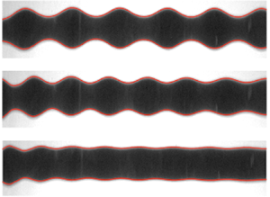
(a) Schematic of the experimental apparatus. (b) Waves  $\omega _0=(0.85,0.95,1.00)/\varOmega$ with fixed amplitude $a=0.8$ but increasing frequencies from left to right. The spatial wave is observed to be periodic in the leftmost image, but get damped in the middle and arrested in the rightmost image. Conduit edges are outlined by the red curves. Measured experimental parameters follows from table 1.

Example fluid properties measured in experiments: viscosities  $\mu ^{(i,e)}$, viscosity ratio $\epsilon$, densities $\rho ^{(i,e)}$, background flow rate $Q_0$, associated conduit diameter $2R_0$ computed by Poiseuille's law, outer wall diameter $2D_0$ and Reynolds numbers $Re^{(i,e)}$ for interior and exterior fluids.

A computer-controlled piston pump is used as a wavemaker to inject the interior fluid into the extrusive fluid at the nozzle that rises buoyantly. Variation in the flow rate results in interfacial waves. Periodic waves are created by a suitable periodic injection rate  $Q^{(i)}(t)$:
 \begin{equation} Q^{(i)}(t)= q(t), \quad t \geqslant 0, \quad q(t+T_0)=q(t), \quad T_0=\frac{2{\rm \pi}}{\omega_0}. \end{equation}
Data acquisition is performed using high-resolution cameras with one (camera 1 in figure 6a) equipped with a macro lens at the injection nozzle for precise data measurement and one to image the far field (camera 2) and capture fully developed periodic wavetrains. Spatial calibration is achieved with a ruler inside the column within the camera view. Example large-amplitude periodic waves generated by time-periodic boundary data with different injection frequencies and the same wave amplitude are shown in figure 6(b). For a relatively small frequency, the periodic wave maintains its fully developed structure, i.e. it propagates. However, by increasing the input frequency, spatial decay of the amplitude is observed. The middle wave is weakly spatially damped and the rightmost wave is arrested at a larger frequency.
4.2. Method
Camera images are processed to extract the conduit edges. A low-pass filter is applied to reduce noise due to pixelation of the photograph and any impurities in the exterior fluid. The conduit diameter is obtained by calculating the number of pixels between the two edges and normalizing by the conduit mean diameter. In each experimental trial, images are taken after the wave has fully developed in the camera view, and we identify  $t=0$ with the initiation of imaging. A $3$ Hz sampling rate for the close camera and a $1$ Hz sampling rate for the full camera were used.
We present all dimensional quantities in tilde notations. The circular cross-sectional area  $\tilde {A}$ of the conduit is then modelled by the dimensional conduit equation
 \begin{equation} \tilde{A}_{\tilde{t}} + \frac{g \varDelta}{8{\rm \pi}\mu^{(i)}} \left( \tilde{A}^2 \right)_{\tilde{z}} - \frac{\mu^{(e)}}{8{\rm \pi} \mu^{(i)}} \left( \tilde{A}^2 \left( \tilde{A}^{{-}1} \tilde{A}_{\tilde{t}}\right) _{\tilde{z}} \right)_{\tilde{z}} =0, \end{equation}
where  $\tilde {z},\tilde {t}$ follow from (2.6) and $\tilde {A} = {\rm \pi}R_0^2 A$. Profile measurements of linear waves are conducted by scaling the data to unit mean and fitting at every temporal and spatial snapshot a sinusoidal plane wave
 \begin{equation} A(\tilde{z},\tilde{t}) = 1+ \frac{a}{2} \cos(\tilde{k} \tilde{z}- \tilde{\omega} \tilde{t} + \psi), \end{equation}
where  $\psi$ represents the phase. The relative $L^2$ norm error in the fit is below $15\,\%$ in space and $10\,\%$ in time. To extract the wavenumber for a trial, we compute the mean of $\tilde {k}$ across a range of times $\tilde {t}$; similarly, the angular frequency is obtained by averaging $\tilde {\omega }$ over a range of heights $\tilde {z}$. The standard error in parameter measurements is roughly as low as $1\,\%$ for $\tilde {k}$ and $0.5\,\%$ for $\tilde {\omega }$, indicating that the fit (4.6) to the data results in a reliable and accurate measurement of linear periodic waves. However, this method is not suitable for waves beyond the linear regime. Instead, larger-amplitude waves with macroscopic edge changes are processed by directly splitting the waves into periods at each snapshot and computing the averaged wavelengths and wave periods. The standard error for $\tilde {k},\tilde {\omega }$ measurements with this technique is typically below $5\,\%$.
To compare the experimental results with theory, we require the vertical length, velocity and time scales  $L,U,T=L/U$ in (2.7a–d) for non-dimensionlization. Upon generation of linear periodic waves, we non-dimensionalize the wavenumber and angular frequency data by using two fitting methods: one is to determine $L_c$ and $U_c$ by fitting the dimensional data $\tilde {\omega },\tilde {k}$ to the conduit linear dispersion relation
 \begin{equation} f(\tilde{k}) = \dfrac{2U_c \tilde{k}}{1+L_c^2 \tilde{k}^2}, \end{equation}
and the other is by fitting  $\tilde {\omega }, \tilde {k}$ with the two-Stokes linear dispersion relation using the spatial $L_S$ and velocity $U_S$ scales, as well as $\epsilon,\lambda$ and $D$. Treating $\epsilon,\lambda$ and $D$ as effective fitting parameters, the two-Stokes linear dispersion relation is determined and fitted to experiments. We note that the fitting method is sensitive to the initial guess for the fitting parameters. These two techniques, which construct a direct relationship between experimental data and theory, return reliable approximations of the dimensional scaling coefficients $L$ and $U$. Differences in the two methods will be discussed in § 4.4. The scales in our experiments from either fitting approach are typically in the range
 \begin{equation} L: 0.3\unicode{x2013}0.4\ \text{cm}, \quad U: 0.3\unicode{x2013}0.4\ \text{cm}\ \text{s}^{{-}1}, \end{equation}
with camera resolutions of  $250{-}400\ \textrm {pixel}\ \textrm {cm}^{-1}$. Although $L$ scales like $R_0/\sqrt {\epsilon }$ for modelling long-wavelength wave dynamics, in our experimental regime, it is comparable to the conduit diameter $2R_0$. Nevertheless, for wavenumbers $0< k \lessapprox 1$, the wavelengths are on the centimetre scale while the conduit diameter is on the scale of millimetres. Prior to each experiment described below, around 10 trials of linear periodic waves were generated for calibrating $L$ and $U$ according to the method described here.
4.3. Definition of linear, weakly nonlinear and fully nonlinear regimes
To categorize the periodic travelling waves obtained in experiments, we perform a preliminary analysis by expressing the spatial waves as a Fourier series at a fixed time  $t=t_0$
 \begin{equation} A(z, t_0) = a_0 + \sum^\infty_{n=1} \frac{a_n}{2} \cos (nk (z - \psi)), \end{equation}
where  $a_0=1$ is the wave mean. Dividing the periodic travelling wave data into periods and applying the Fourier cosine transform, we obtain the Fourier components $a_n$. Fourier components of some selected periodic waves are plotted in figure 7. Waves with negligible second-order and higher modes $|a_n| \ll 0.1$, $n=2,3,\dots$ are identified as lying in the linear regime and can be well described by linear theory. For larger-amplitude waves $( |a_1| \gtrapprox 0.5, |a_2|\gtrapprox 0.1)$, a single harmonic is insufficient and higher-order harmonic terms are needed. A clear distinction between weakly nonlinear and strongly nonlinear waves occurs when the fourth-order coefficient is sufficiently large. The waves with modes $|a_4| \lessapprox 0.1$ are considered to be in the weakly nonlinear regime. On the other hand, the waves with $|a_4| \gtrapprox 0.1$ are in the strongly nonlinear regime, in which case the weakly nonlinear approximation of three harmonics fails. We now assess each wave class beginning with linear waves.
Fourier mode of typical periodic waves in experiments. Waves  $A,B$ with dominant $a_1$ can be approximated by a single sine wave. To describe larger-amplitude waves $C,D$, higher-harmonic terms are needed. Waves $E,F$ with the largest amplitudes acquire non-negligible Fourier modes even at the fourth or fifth order.

4.4. Linear periodic travelling waves
An example linear periodic travelling wave launched in a viscous fluid conduit by the sinusoidal boundary condition  $Q(\tilde {t})=Q_0(1+({a}/{2})\cos (\tilde {\omega } \tilde {t} + {\rm \pi}/2))^2$ for $\tilde {t}>0$ is depicted in figure 8(a). The wave travelling in the positive $\tilde {z}$ direction is periodic in both time and space. Extracting the spatial wave at a fixed time, we fit the periodic wave with a cosine function in figure 8(b). A movie of the linear periodic wave propagation can be found in the supplementary material. This result confirms the prediction from modulation theory that a fully developed periodic wave is generated for input frequency less than the critical value (see (1.11) and (3.3)). Three independent experiments with different fluid properties resulting in three datasets of measured wavenumbers $\tilde {k}$ and wave frequencies $\tilde {\omega }$ were collected. In figure 9, we compare the dimensionless experimental observations of $k(\omega )$ with the conduit linear dispersion relation (1.11). Across all three datasets, good agreement between the experimental data and the theoretical prediction is achieved for sufficiently long wavelengths $\tilde {\zeta }=({2{\rm \pi} }/{k})L_c \gtrapprox 2.3$ cm ( $k<0.8$). The linear dispersion relation of the conduit equation is quantitatively verified in this regime. However, the experimental critical frequency $\omega _{cr}$ and critical wavenumber $k_{cr}$ corresponding to the values between the last datapoint of each dataset in figure 9 and the first point where the wave is damped are subject to a significant shift from 1, the prediction from the conduit equation. The relative discrepancies in $\omega _{cr}$ and $k_{cr}$ are $(\Delta \omega _{cr}, \Delta k_{cr})=(5\,\%, 27\,\%),(7\,\%, 33\,\%), (6\,\%, 29\,\%)$, respectively. It is notable that the observed critical frequency and wavenumber vary across the three datasets where the fluid properties differ. The interior flow rate is calculated using Poiseuille's law and (2.7a–d) for a motionless external fluid so that $Q^{(i)}={\rm \pi} U R_0^2$, where $U=U_c$ is the fitted velocity scale and $R_0$ is the conduit radius measured from experiments. Datasets 1–3 have measured radii $R_0=0.19,0.17,0.18$ cm. As expected for the asymptotic validity of the conduit equation, the vertical wavelength is much larger than the horizontal diameter, i.e. $\tilde {\zeta }\gg 2R_0$. We obtain $Q^{(i)}=2.7,1.7,2.5\ \textrm {ml}\ \min ^{-1}$ for each dataset compared with the nominal input flow rates $Q_0=3.0\pm 0.1, 2.0\pm 0.1, 3.0\pm 0.1\ \textrm {ml}\ \min ^{-1}$, respectively.
(a) Example experimental data of a linear periodic travelling wave in the viscous fluid conduit. Measured wave parameters are  $a=0.12$, $\tilde {k}=1.34\pm 0.04\ \textrm {rad}\ \textrm {cm}^{-1}$ and $\tilde {\omega }=0.86\pm 0.01\ \textrm {rad}\ \textrm {s}^{-1}$. (b) Linear wave data in the spatial domain at $\tilde {t}=39$ s fitted with a sinusoidal waveform. The non-dimensionalization scales are $L=0.35\pm 0.01$ cm and $U=0.39\pm 0.01\ \textrm {cm}\ \textrm {s}^{-1}$.

Fit of the experimental measurements  $k(\omega )$ (dots) to the conduit linear dispersion relation (black curve). Error bars take account of the errors in measurements using (4.6) and errors in non-dimensionalization.

To further interpret the linear periodic waves obtained in experiments and investigate the shorter-wave regime in the neighbourhood of the critical frequency, we compare the experimental results with the linear dispersion relation for two-Stokes interfacial waves (2.14) subject to the assumption  $Q^{(e)}=0$ in (2.9b) so that $\lambda$ follows from (2.11). We fit the experimental data $\tilde {k}(\tilde {\omega })$ in the subcritical regime with the two-Stokes dispersion relation using effective fitting parameters $\epsilon,D$, as well as the scales $L_S$ and $U_S$ to give an exactly matched critical frequency $\omega _{cr}$. Each dataset was collected independently and therefore possesses distinct fluid parameters, although they are all similar. Figure 10 shows the fits and table 2 reports the corresponding $\omega _{cr}$ and $k_{cr}$. It is demonstrated that this fitting procedure results in an upshift in the critical frequency and a downshift in the critical wavenumber. Two-Stokes linear dispersion curves well describe the dispersion relation $k(\omega )$ and provide improved predictions for the critical values. Errors in the critical wavenumber $k_{cr}$ are caused by the step size of the input $\omega$ in experiments, the sensitivity of $k_{cr}$ on fluid parameters and limitations in the fitting method. As $\omega$ approaches $\omega _{cr}$, $k'(\omega )\to \infty$ so that a small change in $\omega$ will lead to a substantial difference in $k$, leading to difficulties in approximating $k_{cr}$. The predicted interior flow rates from the fits using (2.9a) for dataset 1 to 3 are $Q^{(i)}=3.1, 1.9, 2.7\ \textrm {ml}\ \min ^{-1}$, reasonably consistent with the input $Q_0=3.0,2.0,3.0 \ \textrm {ml}\ \min ^{-1}$, and the predicted interior radii obtained from (2.7a–d) are $R_0=0.20, 0.17, 0.18$ cm, respectively. The two-Stokes dispersion relation follows from the physical scenario that we observed in experiments where the interior fluid flows up and pools at the top over time while the exterior flow recirculates with a zero net flow rate.
Experimental results of linear periodic waves  $k(\omega )$ (dots) fitted with the two-Stokes dispersion relation assuming (2.11) (black curve). Insets report predicted recirculating vertical flow velocities.

Comparison of  $\omega _{cr}$ and $k_{cr}$ between experimental measurements and the two-Stokes linear dispersion relation assuming (2.11) (fittings are reported in figure 10). The fitting method requires an exactly correct $\omega _{cr}$. $\Delta k_{cr}$ reports the relative difference of $k_{cr}$.

We have shown that the two-Stokes recirculating flow that includes an external fluid pressure gradient and exterior flow mass conservation is a slightly more accurate model of propagating linear waves generated by a wavemaker than the long-wave conduit equation for describing relatively short waves between two viscous fluids in the linear regime. It is notable, however, that the conduit equation accurately reproduces the subcritical data.
4.5. Linear wave damping and arresting
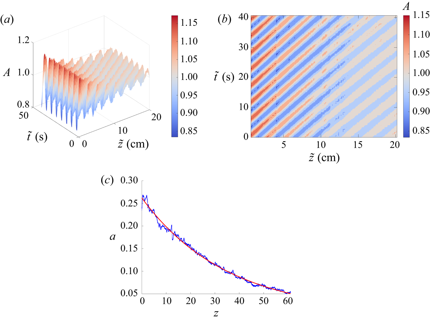
Linear periodic waves in the short-wave, supercritical regime when the injection frequency  $\omega$ exceeds the critical frequency $\omega _{cr}$ exhibit spatial amplitude damping and do not propagate unhindered. Figures 11(a) and 11(b) demonstrate an example of a damped wave observed in a viscous fluid conduit (see the supplementary material for movies). The wave generated by a time-harmonic injection rate at the nozzle quickly decays spatially while maintaining periodicity in time at each fixed spatial location. By measuring the spatial dependence of the amplitude of the wave in figure 11(c), we find that it is well fitted by an exponential function in space. This agrees with our hypothesis derived from the radiation condition (1.11) so that for complex dispersion $k=k_\textrm {Re} + i k_\textrm {Im}$, the plane wave solution takes the form
 \begin{equation} A(z,t) = a \exp({- k_\text{Im} z})\cos(k_\text{Re} z+ \omega t + \psi), \end{equation}
where  $k_\textrm {Im}$ is the spatial damping rate and $k=k(\omega )$ is obtained from the linear dispersion relation in the supercritical regime.
(a) Surface and (b) contour plots of an experimental small-amplitude, damped, non-propagating wave when the injection frequency at the boundary exceeds the critical value. Dimensional wave parameters are  $\tilde {\omega }=1.12\pm 0.03\ \textrm {rad}\ \textrm {s}^{-1}$ and $\tilde {k}=2.32\pm 0.04\ \textrm {rad}\ \textrm {cm}^{-1}$ with scales $L=0.35\pm 0.01$ cm, $U=0.40\pm 0.01\ \textrm {cm}\ \textrm {s}^{-1}$. (c) Amplitude decay (dotted blue) fitted with $a\exp (-bz)$, $a=0.26\pm 0.01$, $b=0.027\pm 0.001$ (solid red).
The exact linear dispersion relation of the conduit equation and the two-Stokes flow system obtained in § 2 are used to compare with the experimental wave profiles. Here, we report the data points in figure 12 as collected using the same experimental set-up as those in figures 9(c) and 10(c); therefore, identical parameters and non-dimensionalization scales are used. No new fitting is applied. For a total of 18 experimental trials,  $k_\textrm {Im}$ is obtained as the spatial amplitude damping rate by fitting an exponential to the wave amplitude, $\omega$ is the averaged frequency over a spatial window size of $z\in [0,2] \to [0,0.7\ \textrm {cm}]$ (250 data points) measured through the cosine fitting method described in § 4.2, and $k_\textrm {Re}$ is the slope of the temporal wave phase over the same spatial window. Figure 12 reports the comparison of the linear dispersion relation in the supercritical regime from experiments and theory. It is shown that the experimental results closely match the two-Stokes theoretical predictions and the first data point of the damping wave is also well approximated by the two-Stokes predicted $\omega _{cr},k_{cr}$. The conduit dispersion relation also performs well at describing $k_\textrm {Im}$ but significantly overshoots $k_\textrm {Re}$.
Comparison between experimental measurements (red dots) of the exponential spatial decay rate (a,c), spatial frequency (b,d) and theory (black line) for waves in the supercritical regime  $\omega >\omega _{cr}$. (a,c) The conduit linear dispersion relation. (b,d) The two-Stokes dispersion relation.

Damped waves are found to exhibit a spatially dependent frequency and wavenumber, as shown in figure 13. Through temporal data fitting with the function  $\phi (t) = a \cos (-\omega t + \psi )$, we obtain the amplitude $a$, frequency $\omega$ and phase $\psi$, whose slope is the real part of the local wavenumber $k_{\textrm {Re}}$. The amplitude fits well to an exponential $\propto e^{-k_\textrm {Im} z}$ that is consistent with linear theory. Additionally, the local temporal $\omega$ and spatial $k_{\textrm {Re}}$ frequencies are also observed to spatially decrease, which we suspect to be a nonlinear effect.
Investigation of a spatially damped wave profile. (a) The amplitude decay is fitted with an exponential function. The decay rate  $b$ is equivalent to $k_{\textrm {Im}}$ in (4.10). (b) The frequency is also found to slightly decrease ( ${\sim }3\,\%$) in space. (c) The real part of the wavenumber is subject to a decay of ${\sim }20\,\%$ in space.

Nevertheless, the conduit equation again provides a reasonable description of part of the supercritical data. We now focus solely on the conduit equation to model nonlinear waves.
4.6. Periodic travelling waves in the weakly nonlinear regime
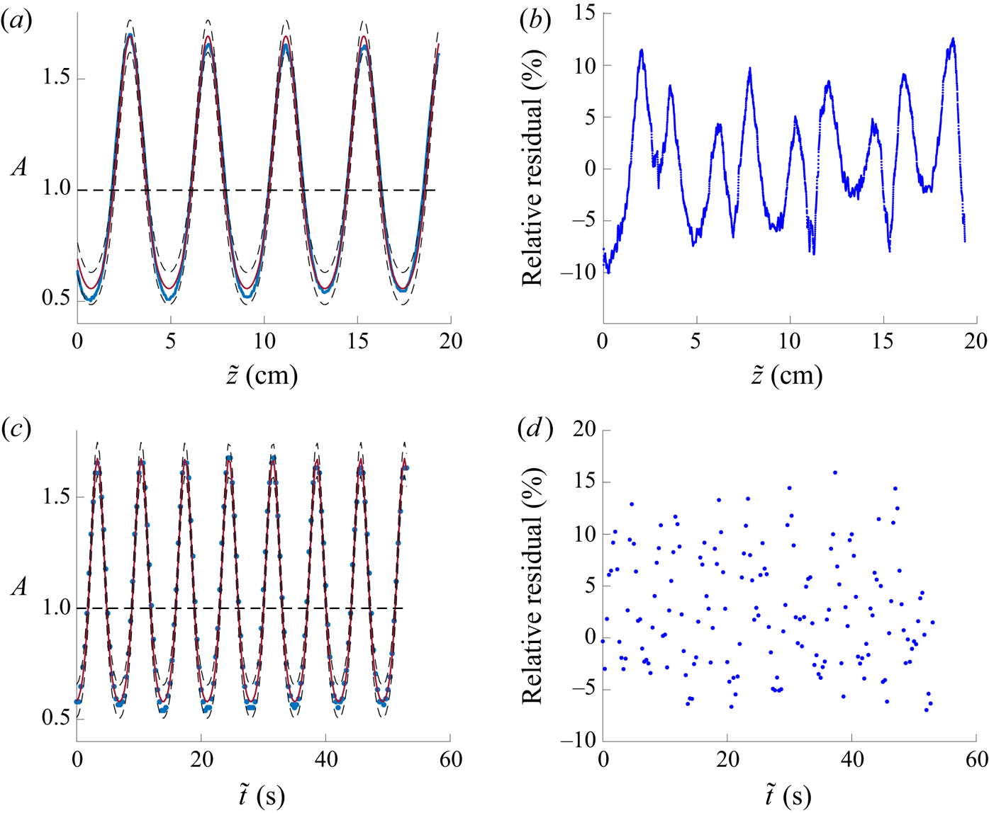
Larger-amplitude, periodic travelling waves in the weakly nonlinear regime are distinguished from their linear counterpart by no longer maintaining symmetry about the wave mean and cannot be described by a single trigonometric harmonic. The waves are more accurately modelled by the weakly nonlinear approximation (1.14a), (1.14b) of the conduit equation obtained via the amplitude expansions  $\phi \sim 1+a\phi _1+a^2\phi _2+a^3\phi _3$ and $k \sim k_0+a^2k_1$, where $0< a\ll 1$ is an amplitude scale. An experimental weakly nonlinear wave is shown in figure 14. Length and velocity scales for non-dimensionalization are $(L_c,U_c)=(0.33 \pm 0.01\ \textrm {cm}, 0.38\pm 0.01\ \textrm {cm}\ \textrm {s}^{-1})$. The dimensional spatial wave in figure 14(a) is fitted with the three harmonic expansion (1.13) at $\tilde {t}=\tilde {t}_0$
 \begin{align} \phi(\tilde{z}) = 1 + \dfrac{a_z}{2} \cos(\tilde{k} \tilde{z} + \psi_1) + \dfrac{1+\tilde{k}^2}{48\tilde{k}^2} a_z^2\cos(2(\tilde{k} \tilde{z} + \psi_1)) + \dfrac{1+\tilde{k}^2}{1536\tilde{k}^4} a_z^3 \cos(3(\tilde{k} \tilde{z}+\psi_1)), \end{align}
where  $a_z=1.10 \pm 0.01$, $k=0.50\pm 0.01$ $(\tilde {k}=1.52\pm 0.01\ \textrm {rad}\ \textrm {cm}^{-1}$) and $\psi _1=2.05\pm 0.01$. The approximate frequency is derived from figure 14(c), where the dimensional temporal wave is approximated by (1.14a) at $\tilde {z}=\tilde {z}_0$
 \begin{align} \phi(\tilde{t}) &= 1 +\frac{a_t}{2}\cos(\tilde{\omega} \tilde{t}+\psi_2)+\frac{a_t^2}{24\left(1-\sqrt{1-\tilde{\omega}^2}\right)}\cos(2(\tilde{\omega} \tilde{t} + \psi_2)) \nonumber\\ &\quad +\frac{\left({-}1-\sqrt{1-\tilde{\omega}^2}\right) a_t^3 }{768\left({-}2+\tilde{\omega}^2+2\sqrt{1-\tilde{\omega}^2}\right)}\cos(3(\tilde{\omega} \tilde{t}+\psi_2)), \end{align}
with  $a_t=1.06 \pm 0.02$, $\omega =0.78\pm 0.01$ ( $\tilde {\omega }=0.90 \pm 0.01\ \textrm {rad}\ \textrm {s}^{-1}$) and $\psi _2=-2.97 \pm 0.03$. The fits exhibit a maximum absolute error of $0.11$ and have larger discrepancies at the wave peaks. Adding higher-order harmonic terms yield an even better approximation.
Measured periodic waves (blue dots) and the weakly nonlinear approximation (red solid lines). Error bars are represented by grey dashed lines and the horizontal black dashed line is the wave mean. (a) The spatial wave at a fixed  $\tilde {t}$ fitted with expansion (4.11). (b) Percentage relative error in space. (c) Wave in the time domain at a fixed $\tilde {z}$ fitted with expansion (4.12). (d) Percentage relative error in time.
A total of 11 trials were measured in the weakly nonlinear regime with the same input amplitude and various input frequencies. Wave profiles are measured as follows. Fitting the spatial and temporal waves with the weakly nonlinear expansions (4.11), (4.12), we obtain dimensionless  $k= \tilde {k} L,\omega =\tilde {\omega }({L}/{U})$ as well as $a=({a_z+a_t})/{2}$ for those 11 trials as the red circles in figure 15. Experimental results are then compared with the weakly nonlinear dispersion relation (1.14b) and the linear dispersion relation (1.10) in figure 15. Although weak nonlinearity does not lead to a significant deviation from the linear dispersion relation, we have shown that the corresponding wave profiles require amplitude-dependent higher harmonics to quantitatively model the experimental observations. We have quantitatively validated the weakly nonlinear approximation for measured conduit periodic travelling waves of sufficiently large amplitude and demonstrated the necessity of including higher-order harmonic terms in this regime.
Non-dimensional experimental wave profiles  $k(\omega )$ (circles) compared with the weakly nonlinear dispersion relation (1.14b) at $a=1.04$ (black solid line) and the linear dispersion relation (blue dashed line).

4.7. Cnoidal-like nonlinear periodic waves
We now investigate periodic travelling waves with large amplitudes in the fully nonlinear regime (see the supplementary material for movies). We refer to these waves as cnoidal like, owing to their similarities to the KdV/BBM cnoidal wave solutions (1.5). First, we generate linear periodic waves for calibrating the scales  $L_c=0.26\pm 0.01$ cm and $U_c=0.25\pm 0.01\ \textrm {cm}\ \textrm {s}^{-1}$. We then utilize a numerical database of pre-computed conduit cnoidal-like solutions (Maiden & Hoefer Reference Maiden and Hoefer2016) to experimentally generate and analyse the observed large-amplitude periodic waves. Waves are generated by varying the injection flow rate according to
 \begin{equation} Q(\tilde{t}) = Q_0\phi^2(- \tilde{\omega} \tilde{t}), \end{equation}
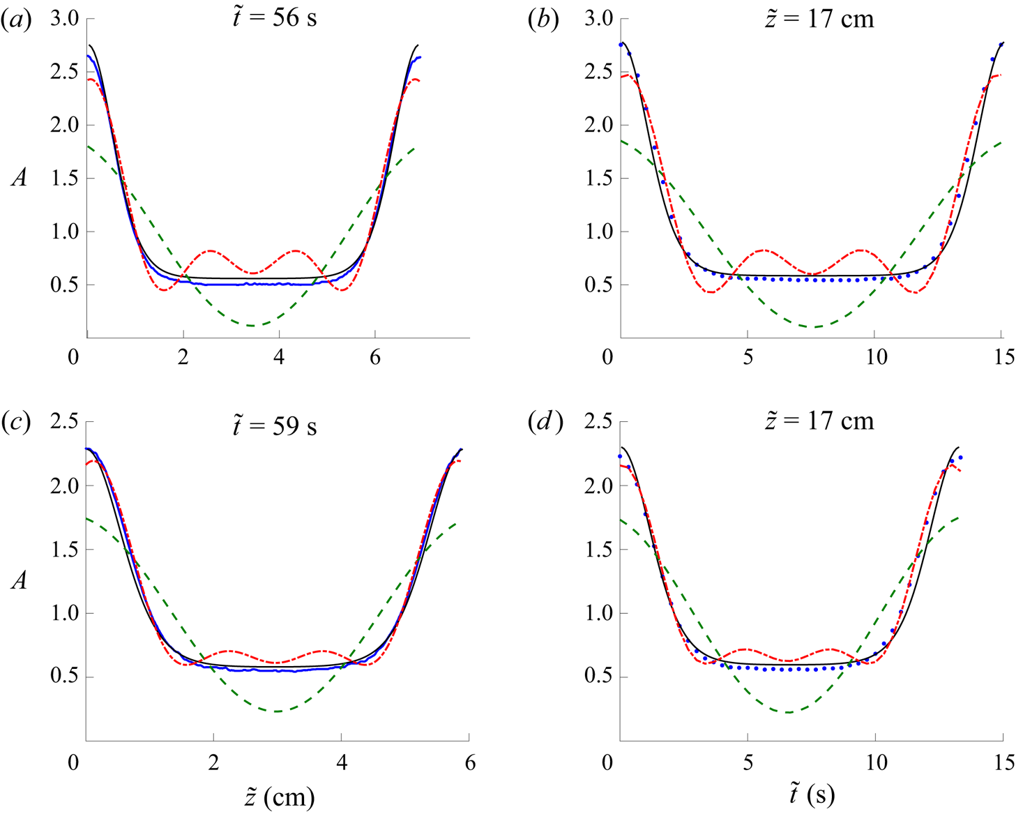
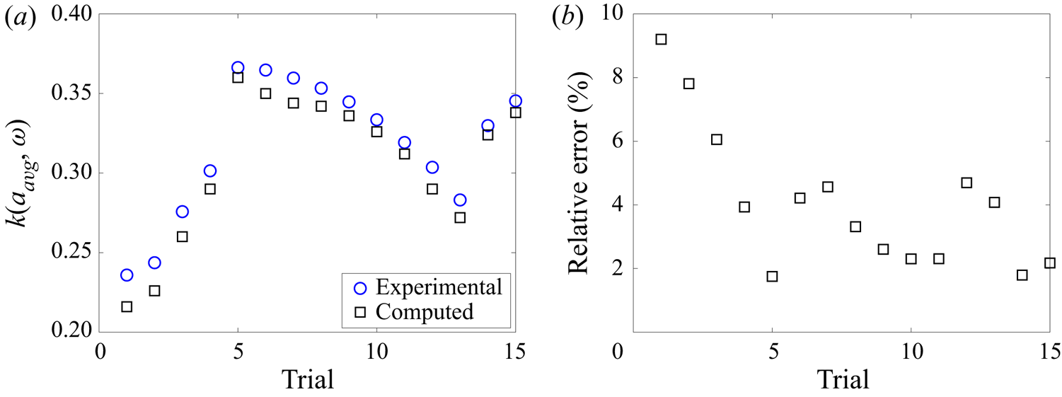
where  $\phi$ is a cnoidal-like solution with unit mean satisfying (1.9). Measured waves are processed by dividing each space and time window into spatial and temporal periods. The average of all processed periods and wave profiles are then reported. Figure 16 displays two example wave profiles, separately in space and time. By direct comparison, it is clear that the observed large-amplitude waves cannot be described by linear or weakly nonlinear approximations. Instead, we compare the observed waves with cnoidal-like solutions to the conduit equation. The amplitude is obtained as $a_z=\max (\phi (z))-\min (\phi (z))$ for waves in the spatial domain, and $a_t=\max (\phi (t))-\min (\phi (t))$ for waves in the temporal domain. Here, $\omega$ and $k$ are measured by the relation $\omega ={2{\rm \pi} }/{\overline {T_0}}$, $k={2{\rm \pi} }/{\bar {\zeta }}$ with non-dimensional averaged time period $\overline {T_0}$ and averaged wavelength $\bar {\zeta }$. The set of unit-mean cnoidal-like solutions is a two-parameter family. Taking $(a_z,k)$ as the parameters for spatial waves and $(a_t,\omega )$ as the parameters for temporal waves, the corresponding cnoidal-like solutions are compared with the experiments in figure 16. The cnoidal-like wave profiles are barely distinguishable from the observed wave profiles. We stress that we have not performed any fitting in this procedure other than the independent determination of the scales $L_c$ and $U_c$ from linear wave dispersion measurements. The cnoidal-like solution of the conduit equation is uniquely selected from the two-parameter family using the extracted $(a_z,k)$ in the spatial case or $(a_t,\omega )$ in the temporal case. No profile fitting was performed. However, discrepancies in spatial and temporal profile measurements lead to $(a_z,k)$ and $(a_t,\omega )$ belonging to two slightly different cnoidal-like solutions for the same trial. We report the average of the two amplitudes $a_{avg}=({a_z+a_t})/{2}$ in table 3. To see how close the solutions are, measurements of wave parameters for 15 trials are reported in table 3 and figure 17.
Averaged experimental wave profiles over one wavelength or period (blue dots) compared with linear (green dashed), weakly nonlinear (red dash-dotted) approximations and cnoidal-like solutions (black solid) in both spatial (a,c) and temporal (b,d) domains. (a,b) The extracted wave parameters are  $(a_{avg},\omega,k)=(2.20,0.44,0.24)$ (trial 1 in figure 17). (c,d) The extracted parameters are $(a_{avg},\omega,k)=(1.71,0.50,0.28)$ (trial 3 in figure 17).
(a) Comparison of the conduit equation nonlinear dispersion relation for cnoidal-like solutions. Data points are from the trials reported in table 3. Utilizing measured  $(a_{avg}, \omega )$ as the parameters, experimental wavenumbers (blue circles) are compared with the numerically computed nonlinear dispersion relation $k(a_{avg},\omega )$ (black squares). (b) Percentage relative error in $k$ for each trial.
Nonlinear periodic wave measurements. Columns 2–4: measured wave parameters. Column 5: numerically computed solution  $k$ at measured $(a_{avg}, \omega )$. Column 6: relative error between experimental $k$ and cnoidal-like wave solutions. Trials 1 and 3 are depicted in figure 16. All trials are shown in figure 17.

The nonlinear dispersion relation  $k(\omega,a_{avg})$ is compared between experiments and cnoidal-like solutions in figure 17. Agreement is quantitatively achieved for all but three trials within $5\,\%$ relative error, with at most $10\,\%$ error otherwise. These measurements are across a range of wave amplitudes $a_{avg} \in (0.89,2.2)$ and frequencies $\omega \in (0.44,0.62)$. The trials in figure 17 are numbered from highest amplitude to lowest, as shown in table 3. Notably, the experimentally measured wavenumbers exceed the predicted values across all 15 trials. Although a different class of waves, we remark that previous measurements of large-amplitude soliton solutions in Olson & Christensen (Reference Olson and Christensen1986) found that the soliton speed was consistently underpredicted by conduit equation soliton solutions. We hypothesize that inclusion of the weakly recirculating flow in the model could improve upon the already good predictions.
5. Discussion and conclusion
The main result of this study is the reliable generation of periodic travelling waves in a viscous fluid conduit across a wide range of amplitudes and long to short wavelengths that are well modelled by the conduit equation. This provides further evidence of the viscous fluid conduit as an accessible and flexible laboratory system for the study of nonlinear wave dynamics with an accurate partial differential equation model in the conduit equation. In order to quantitatively model shorter small-amplitude waves, we found it helpful to derive the full two-Stokes linear dispersion relation that accounts for the actual conditions in our experiment. Radial variation in the vertical velocity allows for a non-negligible exterior pressure gradient and recirculating flow. Together with an outer wall, these two main factors give rise to an upshifted critical frequency for the transition from propagating to non-propagating, spatially damped waves. This upshift from the conduit equation's critical frequency in the short-wave regime is observed and verified quantitatively. The two-Stokes recirculating flow system with exterior flow mass conservation is therefore considered to be a more precise model in which we successfully extend the linear dispersive properties of the model to a shorter-wave regime. The two-Stokes linear dispersion relation is exactly obtained in terms of Bessel functions. Nevertheless, the conduit equation remains an excellent model of propagating linear waves.
Another key result of this experimental investigation is the existence and stability of periodic travelling waves in the fluid conduit wavemaker problem. Low-frequency periodic waves generated at the boundary with a time-periodic injection rate are observed to coherently propagate as travelling waves. Arrested wave propagation for waves generated above the critical injection frequency was observed and found to quantitatively match the two-Stokes dispersion relation for real frequencies and complex wavenumbers. These observations are explained in terms of the radiation condition and linear wave modulation theory.
In addition to presenting a careful analysis of linear periodic waves, our work also contributes to an understanding of conduit periodic travelling waves in the weakly nonlinear and strongly nonlinear regimes. Nonlinear periodic waves are found to require more Fourier harmonics with strongly nonlinear waves well described by cnoidal-like solutions of the conduit equation. Quantitative agreement is achieved between experimental results and conduit cnoidal-like solutions for both the nonlinear dispersion relation and the wave profiles. The characterization of strongly nonlinear periodic travelling waves and their reliable generation in a viscous fluid conduit hold promise for future studies of more general boundary value problems in dispersive hydrodynamics (El & Hoefer Reference El and Hoefer2016), including the generalized Riemann problem and the generation of breathers and breather trains.
Supplementary movies
Supplementary movies are available at https://doi.org/10.1017/jfm.2022.993.
Acknowledgements
The authors thank J. Harris and E. Glenn for their contributions at the beginning of the conduit periodic travelling wave experiments.
Funding
This work was supported by the National Science Foundation (grant number DMS-1816934).
Declaration of interests
The authors report no conflict of interest.
Appendix A. Two-Stokes flow and non-dimensionalization
The governing equations (2.1a) for continuity and momentum conservation will now be non-dimensionalized according to (2.6). Equations for the interior fluid take the non-dimensional form
 $$\begin{gather} \dfrac{1}{r}\dfrac{\partial}{\partial r}(r {u}_r^{(i)}) + \epsilon^{1/2}\dfrac{\partial {u}_z^{(i)}}{\partial z} = 0, \end{gather}$$
 $$\begin{gather}-\epsilon^{{-}3/2}\dfrac{\partial p^{(i)}}{\partial r}+\boldsymbol{\nabla}^2 {u}_r^{(i)}-\epsilon^{{-}1}\dfrac{{u}_r^{(i)}}{r^2} = 0, \end{gather}$$
 $$\begin{gather}-\epsilon^{{-}1}\dfrac{\partial p^{(i)}}{\partial z}+\boldsymbol{\nabla}^2 {u}_z^{(i)} = 0, \end{gather}$$
where  $\boldsymbol{\nabla} ^2=\epsilon ^{-1}({1}/{r})({\partial }/{\partial r})(r({\partial }/{\partial r}))+{\partial ^2}/{\partial z^2}.$ For the exterior fluid, the equations are
 $$\begin{gather} \dfrac{1}{r}\dfrac{\partial}{\partial r}(r u_r^{(e)}) + \epsilon^{1/2}\dfrac{\partial u_z^{(e)}}{\partial z} = 0, \end{gather}$$
 $$\begin{gather}-\epsilon^{{-}1/2}\dfrac{\partial p^{(e)}}{\partial r}+\boldsymbol{\nabla}^2 u_r^{(e)}-\epsilon^{{-}1}\dfrac{u_r^{(e)}}{r^2} = 0, \end{gather}$$
 $$\begin{gather}-\dfrac{\partial p^{(e)}}{\partial z}+\boldsymbol{\nabla}^2 u_z^{(e)} =0. \end{gather}$$
The kinematic boundary condition is
 \begin{equation} \boldsymbol{u}_r^{(i)}=\epsilon^{1/2}\left(\dfrac{\partial R}{\partial t}+\boldsymbol{u}_z^{(i)}\dfrac{\partial R}{\partial z}\right), \quad r=R(z,t). \end{equation}
Equations for continuity of the velocity components are
 $$\begin{gather} (\boldsymbol{u}_r^{(i)}-u_r^{(e)}) =\epsilon^{1/2}\dfrac{\partial R}{\partial z}(\boldsymbol{u}_z^{(i)}-u_z^{(e)}), \quad r=R(z,t), \end{gather}$$
 $$\begin{gather}(u_z^{(e)}-\boldsymbol{u}_z^{(i)}) =\epsilon^{1/2}\dfrac{\partial R}{\partial z}(\boldsymbol{u}_r^{(i)}-u_r^{(e)}), \quad r=R(z,t). \end{gather}$$
The non-dimensional stress balance conditions in the normal and tangential directions are, respectively,
 $$\begin{gather} \left[ -\|\boldsymbol{n}_c\|^2 P + \kappa \left({\boldsymbol{\mathsf{\sigma}}}_{rr}-2\epsilon^{1/2}\dfrac{\partial R}{\partial z}{\boldsymbol{\mathsf{\sigma}}}_{rz}+\epsilon\left(\dfrac{\partial R}{\partial z}\right)^2 {\boldsymbol{\mathsf{\sigma}}}_{zz}\right)\right]_j = 0, \quad r=R(z,t), \end{gather}$$
 $$\begin{gather}\left[ \kappa \left\{ - \left(1-\epsilon\left(\dfrac{\partial R}{\partial z}\right)^2\right) {\boldsymbol{\mathsf{\sigma}}}_{rz} + \epsilon^{1/2} \dfrac{\partial R}{\partial z} ({\boldsymbol{\mathsf{\sigma}}}_{zz}-{\boldsymbol{\mathsf{\sigma}}}_{rr})\right\}\right]_j = 0, \quad r=R(z,t), \end{gather}$$
where  $\kappa ^{(e)}=\epsilon ^{-1}, \kappa ^{(i)}=1$ are the fluid-specific coefficients, $\boldsymbol {n}_c=[\begin {smallmatrix} 1 \\ - \epsilon ^{1/2} {\partial R}/{\partial z} \end {smallmatrix}]$ is the normal vector for the conduit and $P$ is the scaled, absolute pressure with $P^{(i,e)} = p^{(i,e)}-{\rho ^{(i,e)}z}/({\rho ^{(e)}-\rho ^{(i)}})$. The normalized deviatoric stress tensor is
 \begin{equation}
{\boldsymbol{\mathsf{\sigma}}}^{(i,e)}= \begin{bmatrix} {\boldsymbol{\mathsf{\sigma}}}_{rr}^{(i,e)} &
{\boldsymbol{\mathsf{\sigma}}}_{rz}^{(i,e)} \\ {\boldsymbol{\mathsf{\sigma}}}_{zr}^{(i,e)} &
{\boldsymbol{\mathsf{\sigma}}}_{zz}^{(i,e)} \end{bmatrix} = \epsilon^{1/2}
\begin{bmatrix} 2\dfrac{\partial u_r^{(i,e)}}{\partial r} &
\dfrac{\partial u_z^{(i,e)}}{\partial
r}+\epsilon^{1/2}\dfrac{\partial u_r^{(i,e)}}{\partial
z}\\ \dfrac{\partial u_z^{(i,e)}}{\partial
r}+\epsilon^{1/2}\dfrac{\partial u_r^{(i,e)}}{\partial z} &
2\epsilon^{1/2} \dfrac{\partial u_z^{(i,e)}}{\partial z}
\end{bmatrix}.
\end{equation}
\begin{equation}
{\boldsymbol{\mathsf{\sigma}}}^{(i,e)}= \begin{bmatrix} {\boldsymbol{\mathsf{\sigma}}}_{rr}^{(i,e)} &
{\boldsymbol{\mathsf{\sigma}}}_{rz}^{(i,e)} \\ {\boldsymbol{\mathsf{\sigma}}}_{zr}^{(i,e)} &
{\boldsymbol{\mathsf{\sigma}}}_{zz}^{(i,e)} \end{bmatrix} = \epsilon^{1/2}
\begin{bmatrix} 2\dfrac{\partial u_r^{(i,e)}}{\partial r} &
\dfrac{\partial u_z^{(i,e)}}{\partial
r}+\epsilon^{1/2}\dfrac{\partial u_r^{(i,e)}}{\partial
z}\\ \dfrac{\partial u_z^{(i,e)}}{\partial
r}+\epsilon^{1/2}\dfrac{\partial u_r^{(i,e)}}{\partial z} &
2\epsilon^{1/2} \dfrac{\partial u_z^{(i,e)}}{\partial z}
\end{bmatrix}.
\end{equation}
The above non-dimensional governing equations associated with the interfacial boundary conditions, as well as the boundary conditions along the symmetry axis  $\boldsymbol{u}_r^{(i)} = {\partial \boldsymbol{u}_z^{(i)}}/{\partial r} = {\partial p^{(i)}}/{\partial r}=0$ at $r=0$ and the outer wall $u_r^{(e)}=u_z^{(e)}=0$ at $r=D$ provide a complete description of the dynamics of the two-Stokes interfacial flow.
Appendix B. Two-Stokes exact linear dispersion relation
In this section, we derive the solutions for the eigenfunctions in the two-Stokes flow linearization (2.12a)–(2.12d) and compute the exact linear dispersion relation. The differential equations for two-Stokes flow disturbances are
 $$\begin{gather} \dfrac{{\rm d} g_r(r)}{{\rm d}r} +\frac{g_r(r)}{r}+ k g_z(r) =0, \end{gather}$$
 $$\begin{gather}\epsilon g''_r +\frac{ \epsilon g'_r }{r}- k^2 \epsilon ^2 g_r -\frac{ \epsilon g_r }{r^2}+ {\rm i} h'(r) = 0, \end{gather}$$
 $$\begin{gather}g''_z +\frac{g'_z }{r}-k^2 \epsilon g_z -{\rm i} k h(r) = 0 , \end{gather}$$
for the interior fluid on the interval  $0\leqslant r \leqslant \eta$ and
 $$\begin{gather} \dfrac{{\rm d} {G}_r(r)}{{\rm d} r} +\frac{{G}_r(r) }{r}+ k \epsilon {G}_z(r) =0, \end{gather}$$
 $$\begin{gather}{G}_r'' +\frac{{G}_r'}{r} - k^2 \epsilon {G}_r -\frac{{G}_r }{r^2}+ {\rm i} H'(r) = 0, \end{gather}$$
 $$\begin{gather}{G}_z''+\frac{{G}_z'}{r} - k^2 \epsilon {G}_z -{\rm i} k H(r) = 0 , \end{gather}$$
for the exterior fluid on the interval  $\eta \leqslant r \leqslant D$. Along with the interfacial boundary conditions expanded about $r=R(z,t)=\eta +a\exp ({\textrm {i}(kz-\omega t)})$
 $$\begin{gather} k u_{z,0}^{(i)}(\eta) - g_r(\eta) - \omega =0, \end{gather}$$
 $$\begin{gather}\epsilon k u_{z,0}^{(e)}(\eta) - k u_{z,0}^{(i)}(\eta) + g_r(\eta) - {G}_r(\eta) =0, \end{gather}$$
 $$\begin{gather}\epsilon \dfrac{\partial u_{z,0}^{(e)}}{\partial r}(\eta) - \dfrac{\partial u_{z,0}^{(i)}}{\partial r}(\eta) - g_z(\eta) + \epsilon {G}_z(\eta) =0, \end{gather}$$
 $$\begin{gather}-2{\rm i}\epsilon k \dfrac{\partial u_{z,0}^{(e)}}{\partial r}(\eta) + 2{\rm i}\epsilon k \dfrac{\partial u_{z,0}^{(i)}}{\partial r}(\eta) - 2{\rm i}\epsilon g'_r(\eta) +2{\rm i}G'_r(\eta) + h(\eta) - \epsilon H(\eta) =0, \end{gather}$$
 $$\begin{gather}-\dfrac{\partial^2 u_{z,0}^{(e)}}{\partial r^2}(\eta) + \dfrac{\partial^2 u_{z,0}^{(i)}}{\partial r^2}(\eta) - \epsilon k g_r(\eta) + k {G}_r(\eta) + g'_z(\eta) -G'_z(\eta) =0, \end{gather}$$
and  $g_r(0) = 0, g_z'(0) = 0, {G}_r(D) = 0, {G}_z(D) = 0$, the equations can be solved in terms of modified Bessel functions. The internal flow admits the general solution
 \begin{align} g_r(r) &= a_1 K_1\left(\epsilon^{1/2} k r \right) + a_2 I_1\left(\epsilon^{1/2} k r \right) + a_3 r K_0\left(\epsilon^{1/2} k r \right) + a_4 r I_0\left(\epsilon^{1/2} k r \right), \end{align}
 \begin{align} g_z(r) &= a_1 \epsilon^{1/2} K_0\left(\epsilon^{1/2} k r \right) - a_2 \epsilon^{1/2}I_0\left(\epsilon^{1/2} k r \right) - \frac{2a_3}{k}K_0\left(\epsilon^{1/2} k r \right) + a_3 \epsilon^{1/2} r K_1 \left(\epsilon^{1/2} k r \right) \nonumber\\ & \quad - \frac{2a_4}{k} I_0\left(\epsilon^{1/2} k r \right) - a_4 \epsilon^{1/2} r I_1\left(\epsilon^{1/2} k r \right), \end{align}
 \begin{align} {\rm i}h(r) &={-}2\epsilon \left( a_3 K_0\left(\epsilon^{1/2} k r \right) + a_4 I_0\left(\epsilon^{1/2} k r \right) \right). \end{align}
The solution set is linearly independent since the Wronskian  $W=-{4k^2 \epsilon }/{r^2}$ is non-zero. Symmetry along $r=0$ requires $a_1=a_3=0$. Similarly, we obtain the general solution for the extrusive velocities and pressure as
 \begin{align} {G}_r(r) &= b_1 K_1\left(\epsilon^{1/2} k r \right) + b_2 I_1\left(\epsilon^{1/2} k r \right) + b_3 r K_0\left(\epsilon^{1/2} k r \right) + b_4 r I_0\left(\epsilon^{1/2} k r \right), \end{align}
 \begin{align} {G}_z(r) &= \frac{1}{\epsilon} \left[ b_1 \epsilon^{1/2} K_0\left(\epsilon^{1/2} k r \right) - b_2 \epsilon^{1/2}I_0\left(\epsilon^{1/2} k r \right) - \frac{2b_3}{k}K_0\left(\epsilon^{1/2} k r \right) \right. \nonumber\\ & \left.\quad +\, b_3 \epsilon^{1/2} r K_1 \left(\epsilon^{1/2} k r \right)- \frac{2b_4}{k} I_0\left(\epsilon^{1/2} k r \right) - b_4 \epsilon^{1/2} r I_1\left(\epsilon^{1/2} k r \right) \right], \end{align}
 \begin{align} {\rm i}H(r) &={-}2 \left( b_3 K_0\left(\epsilon^{1/2} k r \right) + b_4 I_0\left(\epsilon^{1/2} k r \right) \right). \end{align}
Applying the interfacial boundary conditions and no-slip, no-penetration outer conditions, a linear system is derived for the coefficients  $a_{2,4}, b_{1-4}$
 \begin{equation} \boldsymbol{\mathsf{A}} \begin{pmatrix} a_2 \\ a_4 \\ b_1 \\ b_2\\ b_3 \\ b_4 \end{pmatrix} = \begin{pmatrix} 0\\ -\frac{\eta}{2}(1-\epsilon)(1-\lambda) \\ 0 \\ 1 \\ 0 \\ 0 \end{pmatrix}, \end{equation}
where
 \begin{equation} \boldsymbol{\mathsf{A}}=
\begin{pmatrix} I_1 & I_0 \eta & -K_1 & -I_1 & -K_0 \eta &
-I_0\eta \\ {\mathsf{A}}_{21} & {\mathsf{A}}_{22} & {\mathsf{A}}_{23} & {\mathsf{A}}_{24} & {\mathsf{A}}_{25} &
{\mathsf{A}}_{26} \\ {\mathsf{A}}_{31} & {\mathsf{A}}_{32} & {\mathsf{A}}_{33} & {\mathsf{A}}_{34} & {\mathsf{A}}_{35} &
{\mathsf{A}}_{36} \\ {\mathsf{A}}_{41} & {\mathsf{A}}_{42} & {\mathsf{A}}_{43} & {\mathsf{A}}_{44} & {\mathsf{A}}_{45}, & {\mathsf{A}}_{46}\\
0 & 0 & K_1(\epsilon^{1/2}D k) & I_1(\epsilon^{1/2}D k) & D K_0(\epsilon^{1/2}D k) & D I_0(\epsilon^{1/2}D k) \\
0 & 0 & K_0(\epsilon^{1/2}D k) & - I_0(\epsilon^{1/2}D k) & {\mathsf{A}}_{65} & {\mathsf{A}}_{66} \end{pmatrix}
\end{equation}
\begin{equation} \boldsymbol{\mathsf{A}}=
\begin{pmatrix} I_1 & I_0 \eta & -K_1 & -I_1 & -K_0 \eta &
-I_0\eta \\ {\mathsf{A}}_{21} & {\mathsf{A}}_{22} & {\mathsf{A}}_{23} & {\mathsf{A}}_{24} & {\mathsf{A}}_{25} &
{\mathsf{A}}_{26} \\ {\mathsf{A}}_{31} & {\mathsf{A}}_{32} & {\mathsf{A}}_{33} & {\mathsf{A}}_{34} & {\mathsf{A}}_{35} &
{\mathsf{A}}_{36} \\ {\mathsf{A}}_{41} & {\mathsf{A}}_{42} & {\mathsf{A}}_{43} & {\mathsf{A}}_{44} & {\mathsf{A}}_{45}, & {\mathsf{A}}_{46}\\
0 & 0 & K_1(\epsilon^{1/2}D k) & I_1(\epsilon^{1/2}D k) & D K_0(\epsilon^{1/2}D k) & D I_0(\epsilon^{1/2}D k) \\
0 & 0 & K_0(\epsilon^{1/2}D k) & - I_0(\epsilon^{1/2}D k) & {\mathsf{A}}_{65} & {\mathsf{A}}_{66} \end{pmatrix}
\end{equation}
with  $I_0 = I_0(\epsilon ^{1/2} \eta k)$, $I_1 = I_1(\epsilon ^{1/2} \eta k)$, $K_0 = K_0(\epsilon ^{1/2} \eta k)$, $K_1 = K_1(\epsilon ^{1/2} \eta k)$ and
 \begin{align} \left.\begin{gathered} {\mathsf{A}}_{21} = \epsilon^{1/2} I_0, \quad {\mathsf{A}}_{22} = 2\frac{I_0}{k}+ \epsilon^{1/2} I_1 \eta, \quad {\mathsf{A}}_{23} = \epsilon^{1/2}K_0, \\ {\mathsf{A}}_{24} ={-}\epsilon^{1/2} I_0, \quad {\mathsf{A}}_{25} ={-}2\frac{K_0}{k} + \epsilon^{1/2} K_1 \eta, \quad {\mathsf{A}}_{26} ={-}2\frac{I_0}{k}-\epsilon^{1/2}I_1 \eta, \\ {\mathsf{A}}_{31} = \frac{2}{\eta}\left(-\epsilon I_1 + \epsilon^{3/2}I_0 k \eta \right), \quad {\mathsf{A}}_{32} = 2 \epsilon^{3/2} I_1 k \eta , \quad {\mathsf{A}}_{33} = \frac{2}{\eta}\left(K_1 + \epsilon^{1/2} K_0 k\eta \right), \\ {\mathsf{A}}_{34} = \frac{2}{\eta}\left(I_1 - \epsilon^{1/2} I_0 k\eta \right), \quad {\mathsf{A}}_{35} = 2 \epsilon^{1/2} K_1 k \eta, \quad {\mathsf{A}}_{36} ={-}2\epsilon^{1/2} I_1 k\eta, \\ {\mathsf{A}}_{41} ={-}2\epsilon I_1 k, \quad {\mathsf{A}}_{42} ={-}2\epsilon^{1/2} I_1 - 2\epsilon I_0 k\eta, \quad {\mathsf{A}}_{43} = 2K_1 k , \\ {\mathsf{A}}_{44} = 2I_1 k, \quad {\mathsf{A}}_{45} ={-}\frac{2}{\epsilon^{1/2}} K_1 + 2K_0 k\eta, \quad {\mathsf{A}}_{46} = \frac{2I_1}{\epsilon^{1/2}} + 2I_0 k \eta,\\ {\mathsf{A}}_{65} = \frac{1}{\epsilon^{1/2} k}\left({-}2K_0(\epsilon^{1/2}D k) + \epsilon^{1/2} D k K_1(\epsilon^{1/2}D k) \right), \\ {\mathsf{A}}_{66} = \frac{1}{\epsilon^{1/2} k} \left({-}2I_0(\epsilon^{1/2}D k) - \epsilon^{1/2} D k I_1(\epsilon^{1/2}D k) \right). \end{gathered}\right\} \end{align}
Varying  $\epsilon, D$ leads to changes in the dispersion curves from the conduit dispersion relation as well as changes in the critical frequency $\omega _{cr}$, critical wavenumber $k_{cr}$ and inflection point $k_{inf}$ (see figure 18).
Investigation of (a) the critical frequency  $\omega _{cr}$, (b) the critical wavenumber $k_{cr}$ and (c) the inflection point $k_{inf}$ at selected parameters $\epsilon,D$ for recirculating flow (2.11).

Following the asymptotic behaviour  $D=\epsilon ^{-1/2} d$ and $\lambda = \epsilon ({16}/{d^2}) + O(\epsilon ^2 \ln (\epsilon ))$, where $d=O(1)$, we expand the modified Bessel functions in the linear system (B6) for $\epsilon \to 0$. We seek solutions to the system (B6) with the asymptotic expansions
 \begin{equation} \boldsymbol{v} =
\begin{pmatrix} a_2 \\ a_4 \\ b_1 \\ b_2\\ b_3 \\ b_4
\end{pmatrix}
= \begin{pmatrix} \epsilon^{{-}3/2}
\left(a_{20}+ \epsilon \ln(\epsilon) a_{21} + \epsilon
a_{22} + \epsilon^2 \ln(\epsilon) a_{23} + \epsilon^2
a_{24} + \dots \right) \\
\epsilon^{{-}1} \left( a_{40}+
\epsilon \ln(\epsilon) a_{41} + \epsilon a_{42} +
\epsilon^2 \ln(\epsilon) a_{43} + \epsilon^2 a_{44} + \dots \right) \\
\epsilon^{1/2} \left( b_{10}+ \epsilon
\ln(\epsilon) b_{11} + \epsilon b_{12} + \epsilon^2
\ln(\epsilon) b_{13} + \epsilon^2 b_{14} + \dots \right) \\
\epsilon^{1/2} \left( b_{20}+ \epsilon \ln(\epsilon) b_{21}
+ \epsilon b_{22} + \epsilon^2 \ln(\epsilon) b_{23} +
\epsilon^2 b_{24} + \dots \right) \\
\epsilon \left(b_{30}+ \epsilon \ln(\epsilon) b_{31} + \epsilon b_{32} +
\epsilon^2 \ln(\epsilon) b_{33} + \epsilon^2 b_{34} + \dots \right) \\
\epsilon \left( b_{40}+ \epsilon \ln(\epsilon)
b_{41} + \epsilon b_{42} + \epsilon^2 \ln(\epsilon) b_{43}
+ \epsilon^2 b_{44} + \dots \right) \end{pmatrix}.
\end{equation}
\begin{equation} \boldsymbol{v} =
\begin{pmatrix} a_2 \\ a_4 \\ b_1 \\ b_2\\ b_3 \\ b_4
\end{pmatrix}
= \begin{pmatrix} \epsilon^{{-}3/2}
\left(a_{20}+ \epsilon \ln(\epsilon) a_{21} + \epsilon
a_{22} + \epsilon^2 \ln(\epsilon) a_{23} + \epsilon^2
a_{24} + \dots \right) \\
\epsilon^{{-}1} \left( a_{40}+
\epsilon \ln(\epsilon) a_{41} + \epsilon a_{42} +
\epsilon^2 \ln(\epsilon) a_{43} + \epsilon^2 a_{44} + \dots \right) \\
\epsilon^{1/2} \left( b_{10}+ \epsilon
\ln(\epsilon) b_{11} + \epsilon b_{12} + \epsilon^2
\ln(\epsilon) b_{13} + \epsilon^2 b_{14} + \dots \right) \\
\epsilon^{1/2} \left( b_{20}+ \epsilon \ln(\epsilon) b_{21}
+ \epsilon b_{22} + \epsilon^2 \ln(\epsilon) b_{23} +
\epsilon^2 b_{24} + \dots \right) \\
\epsilon \left(b_{30}+ \epsilon \ln(\epsilon) b_{31} + \epsilon b_{32} +
\epsilon^2 \ln(\epsilon) b_{33} + \epsilon^2 b_{34} + \dots \right) \\
\epsilon \left( b_{40}+ \epsilon \ln(\epsilon)
b_{41} + \epsilon b_{42} + \epsilon^2 \ln(\epsilon) b_{43}
+ \epsilon^2 b_{44} + \dots \right) \end{pmatrix}.
\end{equation}Collecting (B6) with (B9) at each order and applying the kinematic boundary condition (B3a), we achieve the asymptotic expression (2.17) for the linear dispersion relation with
 \begin{align} \omega_2(k) &= 4k \left({-}1+\ln\left(\frac{d}{2\sqrt{2}}\right) \right) - \frac{\sqrt{2}k(1+2k^2)}{1+k^2} b_{20} - 2\sqrt{2} b_{40} \nonumber\\ & \quad + \frac{2k}{3d^2(1+k^2)^2} \left[ d^2 \left(6 \varGamma \left(k^4-2 k^2-1\right)\right. \right. \nonumber\\ & \quad \left.+\,k^4 (\ln (8)-19)-6 k^2 (4+\ln (2))-6-\ln (8)\right) \nonumber\\ &\quad \left.+\, 6 d^2 \left(k^4-2 k^2-1\right) \ln (k)-48\left(k^2+1\right) \right], \end{align}
where  $\varGamma$ is the Euler–Mascheroni constant ( $0.5772\ldots$) and the coefficients are
 \begin{equation}
\left.\begin{gathered} b_{10}
={-}\frac{4\sqrt{2}k^2}{1+k^2},\\ b_{20} = \frac{\begin{array}{@{}c@{}}I_0(d k)
\left(K_1(d k) \left(d^2 k b_{30}+2 b_{10}\right)+d k
b_{10} K_0(d k)\right)+d k I_1(d k) (b_{10} K_1(d k)\\
\qquad +\,d b_{30} K_0(d k))\end{array}}{d k I_0(d k){}^2-2 I_1(d k) I_0(d k)-d k
I_1(d k){}^2},\\ b_{30}
={-}\frac{\sqrt{2}k(1+3k^2)}{1+k^2}, \\
b_{40} ={-}\frac{\begin{array}{c}kI_0(d k) (b_{10} K_1(d k)+d b_{30} K_0(d k))+I_1(d k)
(K_0(d k) (k b_{10}-2 b_{30})\\
\qquad +\,d k b_{30} K_1(d k))\end{array}}{d k
I_0(d k){}^2-2 I_1(d k) I_0(d k)-d k I_1(d k){}^2}.
\end{gathered}\right\}
\end{equation}
\begin{equation}
\left.\begin{gathered} b_{10}
={-}\frac{4\sqrt{2}k^2}{1+k^2},\\ b_{20} = \frac{\begin{array}{@{}c@{}}I_0(d k)
\left(K_1(d k) \left(d^2 k b_{30}+2 b_{10}\right)+d k
b_{10} K_0(d k)\right)+d k I_1(d k) (b_{10} K_1(d k)\\
\qquad +\,d b_{30} K_0(d k))\end{array}}{d k I_0(d k){}^2-2 I_1(d k) I_0(d k)-d k
I_1(d k){}^2},\\ b_{30}
={-}\frac{\sqrt{2}k(1+3k^2)}{1+k^2}, \\
b_{40} ={-}\frac{\begin{array}{c}kI_0(d k) (b_{10} K_1(d k)+d b_{30} K_0(d k))+I_1(d k)
(K_0(d k) (k b_{10}-2 b_{30})\\
\qquad +\,d k b_{30} K_1(d k))\end{array}}{d k
I_0(d k){}^2-2 I_1(d k) I_0(d k)-d k I_1(d k){}^2}.
\end{gathered}\right\}
\end{equation}


 Open access

