


1. Introduction
Stellarators are inherently steady-state plasma confinement devices, which is among the key reasons behind their renaissance as promising candidates for fusion power plants. Ideal magnetohydrodynamic (MHD) equilibria are a central part of optimising the complex, three-dimensional plasma shapes which is a necessary condition for steady-state operation of such devices. The equilibrium magnetic field is required not only in optimisation, but also plays a role in future real-time control algorithms and simulation frameworks (Schissel, Nazikian & Gibbs Reference Schissel, Nazikian and Gibbs2025).
Solving the three-dimensional MHD equations requires numerical approaches, because no analytical solution throughout the full volume of strongly shaped toroidal ideal MHD equilibria with nested magnetic topology exists yet (Bruno & Laurence Reference Bruno and Laurence1996). Recent work advanced analytical models for Fourier components of the equilibrium magnetic field in a subset of reactor-relevant magnetic fields and analytical expansions close to the magnetic axis are used extensively in research (Nikulsin et al. Reference Nikulsin, Sengupta, Jorge and Bhattacharjee2024; Sengupta et al. Reference Sengupta, Rodriguez, Jorge, Landreman and Bhattacharjee2024). These analytical solutions and the following numerical solvers assume a nested magnetic topology, or integrability throughout the volume, and computation of chaotic regions or magnetic islands takes considerably more effort (Hudson et al. Reference Hudson, Dewar, Dennis, Hole, McGann, Von Nessi and Lazerson2012).
Accuracy of numerical partial differential equation (PDE) solutions is inherently connected to the representation which defines gradients, and commonly used ideal MHD equilibrium solvers with nested magnetic field topology can be differentiated accordingly: a widely used finite-difference solver employed in the design of currently operating stellarator devices is VMEC (Hirshman & Whitson Reference Hirshman and Whitson1983), another pseudo-spectral solver is DESC (Dudt & Kolemen Reference Dudt and Kolemen2020) and a third example is GVEC (Hindenlang, Plunk & Maj Reference Hindenlang, Plunk and Maj2025), that abstracts the notion of basis functions, which enabled computation of plasmas with a figure-8 shape (Plunk et al. Reference Plunk, Drevlak, Rodríguez, Babin, Goodman and Hindenlang2025).
Active control of stellarator plasmas is much less required than active control of tokamaks, which are prone to disruptive events that can damage the machine because confinement in tokamaks is dependent on large toroidal plasma currents (Schissel et al. Reference Schissel, Nazikian and Gibbs2025). Modern control policies enabled accurate tracking of the location, current and shape of axisymmetric plasmas realisable within the Tokamak à Configuration Variable device (Degrave et al. Reference Degrave2022). This shows that digital twins and real-time control can also be helpful tools in future stellarator devices, especially regarding control of transport and turbulence and possibly accessing novel plasma states by careful search in a device’s configuration space. Many transport and turbulence codes, and accordingly their surrogate models, rely on either a coordinate system in which the magnetic field lines are straight (Mandell et al. Reference Mandell, Dorland, Abel, Gaur, Kim, Martin and Qian2024) or the equilibrium magnetic field (Landreman et al. Reference Landreman, Smith, Mollén and Helander2014). Computation of straight-field line coordinate systems requires the equilibrium magnetic field and models with very rapid inference of the equilibrium field will be helpful in sophisticated stellarator control strategies. Furthermore, real-time interpretation of diagnostic data is facilitated if the inference time of magnetic equilibria is reduced as much as possible (Merlo et al. Reference Merlo, Böckenhoff, Schilling, Lazerson and Pedersen2023b ).
Artificial neural networks (NNs) enable quick inference by transferring the bulk of the computation to training the NN, which is then composed of simple nonlinearities and parallelisable matrix multiplications.
We introduce simple NN-based models with low residuals over parametrised spaces of equilibria within fixed boundaries and with fixed rotational transform. These models are parametrised by a unit interval scalar multiplier of the pressure coefficients and achieve volume-average force residuals very close to DESC’s force residual over the whole interval, from near-vacuum conditions to full pressure.
1.1. Motivation
This work takes the next step on the path to precise operator models of a subset of fusion relevant ideal MHD equilibria by integrating NNs into DESC. Previous work presented advantages of small multilayer perceptrons (MLPs) which output Fourier decomposed equilibrium magnetic fields (Thun et al. Reference Thun, Merlo, Conlin, Panici and Böckenhoff2026) and we test the same approach in DESC’s Fourier Zernike basis.
DESC can solve equilibria prescribed with current or rotational transform, includes many features such as omnigenous field optimisation (Dudt et al. Reference Dudt, Goodman, Conlin, Panici and Kolemen2024) and Mercier stability (Panici et al. Reference Panici, Conlin, Dudt, Unalmis and Kolemen2023) and has implemented interfaces to gyrokinetic turbulence codes (Kim et al. Reference Kim2024) – all this is immediately available to evaluate operator models parametrised by NNs in future work. The implementation of DESC allows for easy integration of NNs and DESC’s optimisation subspace, in which linear constraints are satisfied by construction, and reduces the dimensionality of the minimisation problem. We train narrow operator models in DESC’s optimisation subspace ( $\boldsymbol{y}$
in (2.17)) using only the force residual evaluated on typical concentric grids at discrete multipliers of the pressure coefficients.
$\boldsymbol{y}$
in (2.17)) using only the force residual evaluated on typical concentric grids at discrete multipliers of the pressure coefficients.
Operator models that parametrise equilibria with low normalised force error are the scaffolding for digital twins, real-time control algorithms and rapid interpretation of diagnostic data. Furthermore, precise equilibrium operator models of the configuration space of a machine are necessary to create sophisticated real-time capable simulation frameworks, for example, including transport and turbulence operator models which use deviations from the equilibrium magnetic field (Schissel et al. Reference Schissel, Nazikian and Gibbs2025).
Another application for the presented operator models is in optimisation: parametrised operator models ensure low sensitivity of stellarator optimisation targets towards uncertainty in the prescribed pressure profile. The presented models are a first step towards parametrisation of flexible configurations that preserve low optimisation metrics throughout a device’s operational limits and map out the landscape of said metrics.
In terms of flight simulators or digital twins, control is likely to benefit from such models: once trained, they can better inform control algorithms by rapidly propagating aleatoric uncertainties through the magnetic field topology to the control algorithm. Models with rapid inference of plasma evolution are expected to play an important role in sophisticated control strategies of advanced fusion experiments (Schissel et al. Reference Schissel, Nazikian and Gibbs2025).
Prior research determined that the minimum size, or complexity, of simple MLPs which parametrise a single ideal MHD equilibrium in Fourier space necessitate two hidden layers, each with a nonlinear activation function (Thun et al. Reference Thun, Merlo, Conlin, Panici and Böckenhoff2026). In the following, we will use this result to answer whether similar two-layer MLPs are also capable of reproducing narrow regions of the ideal MHD PDE operator defined by a scaling factor of the pressure, while keeping the plasma boundary and the rotational transform profile constant. Because we only vary the pressure in this work, we will call these models narrow operator models in the sense that they parametrise a narrow subspace of the ideal MHD PDE.
2. Three-dimensional ideal magnetohydrostatic problem
Stationary points of the ideal MHD PDE with isotropic pressure $p$
describe plasmas as fluids with one species only in the limit of long wavelengths, low frequencies and no electric resistivity (Freidberg Reference Freidberg2014)
$p$
describe plasmas as fluids with one species only in the limit of long wavelengths, low frequencies and no electric resistivity (Freidberg Reference Freidberg2014)
 \begin{align} \boldsymbol{J} \times \boldsymbol{B} &= \boldsymbol{\boldsymbol{\nabla }} \boldsymbol{p}, \end{align}
 \begin{align} \mu _{\mathrm{0}} \boldsymbol{J} &= \boldsymbol{\boldsymbol{\nabla }} \times \boldsymbol{B}, \end{align}
 \begin{align} \boldsymbol{\boldsymbol{\nabla }} \boldsymbol{\boldsymbol{\cdot }} \boldsymbol{B} &= 0, \end{align}
with the magnetic field $\boldsymbol{B}$
, currents
$\boldsymbol{B}$
, currents $\boldsymbol{J}$
, pressure
$\boldsymbol{J}$
, pressure $\boldsymbol{p}$
and vacuum permeability
$\boldsymbol{p}$
and vacuum permeability $\mu_0$
. Inserting Ampère’s law (2.2) into the momentum (2.1) removes currents from this system of equations, yielding the residual force
$\mu_0$
. Inserting Ampère’s law (2.2) into the momentum (2.1) removes currents from this system of equations, yielding the residual force $\boldsymbol{F}$
 \begin{align} (\boldsymbol{\boldsymbol{\nabla }} \times \boldsymbol{B}) \times \boldsymbol{B} &= \mu _{\mathrm{0}} \, {\boldsymbol{\boldsymbol{\nabla }}} \boldsymbol{p} \nonumber \\ \Leftrightarrow \boldsymbol{F} &= (\boldsymbol{\boldsymbol{\nabla }} \times \boldsymbol{B}) \times \boldsymbol{B} - \mu _{\mathrm{0}} \, {\boldsymbol{\boldsymbol{\nabla }}}\boldsymbol{p}\nonumber \\ \Leftrightarrow \boldsymbol{F} &= F_\rho \boldsymbol{\boldsymbol{\nabla }}\rho + F_\theta \boldsymbol{\boldsymbol{\nabla }} \theta + F_\theta \boldsymbol{\boldsymbol{\nabla }} \zeta. \end{align}
Equilibrium states are defined by the magnetic field, which has toroidal, or ring-shaped, form for magnetically confined plasmas in tokamaks and stellarators.
Under the assumption of a nested, or integrable, structure of this magnetic field, the component in radial direction $\rho$
of the magnetic field
$\rho$
of the magnetic field $B^\rho =\boldsymbol{B}\boldsymbol{\boldsymbol{\cdot }} \boldsymbol{\boldsymbol{\nabla }} \rho$
is
$B^\rho =\boldsymbol{B}\boldsymbol{\boldsymbol{\cdot }} \boldsymbol{\boldsymbol{\nabla }} \rho$
is $0$
, and we can write the magnetic field as
$0$
, and we can write the magnetic field as
 \begin{align} \boldsymbol{B} = \boldsymbol{\boldsymbol{\nabla }} \zeta \times \boldsymbol{\boldsymbol{\nabla }} \chi + \boldsymbol{\boldsymbol{\nabla }} \psi \times \boldsymbol{\boldsymbol{\nabla }} \theta ^{\star }= B^\theta \boldsymbol{e}_\theta + B^\zeta \boldsymbol{e}_{\zeta } , \end{align}
with toroidal magnetic flux $2\pi \psi$
and poloidal magnetic flux
$2\pi \psi$
and poloidal magnetic flux $2\pi \chi$
. The radial magnetic coordinate in this work is the same as DESC’s
$2\pi \chi$
. The radial magnetic coordinate in this work is the same as DESC’s $\rho = \sqrt{s} = \sqrt{\psi / \psi_{\mathrm{b}}} \in \mathbb{R} \cap [0,1), \psi_{\mathrm{b}} := \psi(\rho=1)$
,
$\rho = \sqrt{s} = \sqrt{\psi / \psi_{\mathrm{b}}} \in \mathbb{R} \cap [0,1), \psi_{\mathrm{b}} := \psi(\rho=1)$
, $\theta ^\star \in [0, 2\pi]$
is a poloidal angle which straightens magnetic field lines and the magnetic toroidal angle
$\theta ^\star \in [0, 2\pi]$
is a poloidal angle which straightens magnetic field lines and the magnetic toroidal angle $\zeta \in [0, 2\pi]$
is equal to the cylindrical toroidal angle (Helander Reference Helander2014) where
$\zeta \in [0, 2\pi]$
is equal to the cylindrical toroidal angle (Helander Reference Helander2014) where $s$
is the fraction of
$s$
is the fraction of $\psi$
and
$\psi$
and $\psi_{\mathrm{b}}$
.
$\psi_{\mathrm{b}}$
.
Nestedness of the magnetic topology implies constant toroidal and poloidal magnetic flux on isobaric flux surfaces. Assuming nested flux surfaces, the ideal MHD equilibrium equations can be solved in an inverse manner, i.e. they are fully defined by the map from independent to cylindrical laboratory coordinates $[\rho , \theta , \zeta ]^{\mathsf{T}} \rightarrow [R, \lambda , Z]^{\mathsf{T}}$
and three invariants (Hirshman & Whitson Reference Hirshman and Whitson1983).
$[\rho , \theta , \zeta ]^{\mathsf{T}} \rightarrow [R, \lambda , Z]^{\mathsf{T}}$
and three invariants (Hirshman & Whitson Reference Hirshman and Whitson1983).
Under Gauss’s law for magnetism, the contravariant $\boldsymbol{B}$
-field reduces to
$\boldsymbol{B}$
-field reduces to
 \begin{align} \boldsymbol{B}=\, \frac {\partial _\rho \psi }{\sqrt {g}} \left ((\iota (\rho ) \, - \, \partial _\zeta \lambda ) \boldsymbol{e}_{\theta } + (1+\partial _\theta \lambda ) \boldsymbol{e}_{\zeta }\right )\!. \end{align}
Because the poloidal angle $\theta \in [0, 2\pi]$
is arbitrary, as long as it is periodic and the Jacobian of the inverse map stays finite and does not switch sign,
$\theta \in [0, 2\pi]$
is arbitrary, as long as it is periodic and the Jacobian of the inverse map stays finite and does not switch sign, $\lambda$
is introduced as a periodic renormalisation function which straightens magnetic field lines:
$\lambda$
is introduced as a periodic renormalisation function which straightens magnetic field lines: $\theta ^{\star } = \theta + \lambda (\rho ,\theta ,\zeta )$
.
$\theta ^{\star } = \theta + \lambda (\rho ,\theta ,\zeta )$
.
Hirshman & Whitson (Reference Hirshman and Whitson1983) defined the covariant basis vectors of the inverse map as
 \begin{align} \boldsymbol{e}_\rho =\left [\begin{array}{c} \partial _\rho R \\ 0 \\ \partial _\rho Z \end{array}\right ] \quad \boldsymbol{e}_{\theta }=\left [\begin{array}{c} \partial _{\theta } R \\ 0 \\ \partial _{\theta } Z \end{array}\right ] \quad \boldsymbol{e}_{\zeta }=\left [\begin{array}{c} \partial _{\zeta } R \\ R \\ \partial _{\zeta } Z \end{array}\right ]\!, \end{align}
in conjunction with the Jacobian
 \begin{equation} \sqrt {g}=\boldsymbol{e}_s \boldsymbol{\boldsymbol{\cdot }} \boldsymbol{e}_\theta \times \boldsymbol{e}_\zeta =(\boldsymbol{e}^s \boldsymbol{\boldsymbol{\cdot }} \boldsymbol{e}^{\theta } \times \boldsymbol{e}^\zeta )^{-1}. \end{equation}
And the contravariant basis vectors are $\boldsymbol{e}^i = \boldsymbol{\boldsymbol{\nabla }} i = {\boldsymbol{e}_j \times \boldsymbol{e}_k}/{\sqrt {g}}$
with
$\boldsymbol{e}^i = \boldsymbol{\boldsymbol{\nabla }} i = {\boldsymbol{e}_j \times \boldsymbol{e}_k}/{\sqrt {g}}$
with $(i, j, k)$
a cyclic permutation in
$(i, j, k)$
a cyclic permutation in $\{\rho , \theta , \zeta \}$
.
$\{\rho , \theta , \zeta \}$
.
The last components required for solving (2.1) to (2.3) are three invariants: any equilibrium needs some prescribed (isotropic) pressure profile $p(\rho )$
, a rotational transform profile
$p(\rho )$
, a rotational transform profile $\iota (\rho )$
or some current profile
$\iota (\rho )$
or some current profile $c(\rho )$
(Hirshman & Meier Reference Hirshman and Meier1985), and optionally, the plasma boundary can be enforced via
$c(\rho )$
(Hirshman & Meier Reference Hirshman and Meier1985), and optionally, the plasma boundary can be enforced via $R(\rho =1)=R_{\mathrm{b}}$
and
$R(\rho =1)=R_{\mathrm{b}}$
and $Z(\rho =1)=Z_{\mathrm{b}}$
, in which case the equilibrium is called fixed boundary (Kruskal & Kulsrud Reference Kruskal and Kulsrud1958). Additionally, the total toroidal flux through the torus
$Z(\rho =1)=Z_{\mathrm{b}}$
, in which case the equilibrium is called fixed boundary (Kruskal & Kulsrud Reference Kruskal and Kulsrud1958). Additionally, the total toroidal flux through the torus $\psi _{\mathrm{b}}$
can be either specified or set to
$\psi _{\mathrm{b}}$
can be either specified or set to $1 \, \mathrm{Wb}$
with later rescaling of other values.
$1 \, \mathrm{Wb}$
with later rescaling of other values.
Finally, the output is an equilibrium magnetic field $\boldsymbol{B}$
, determined by a balance between plasma pressure gradient and Lorentz force under the assumption of nested magnetic surfaces inside a fixed plasma boundary. The relative strength of both forces is commonly described by a ratio, the plasma beta
$\boldsymbol{B}$
, determined by a balance between plasma pressure gradient and Lorentz force under the assumption of nested magnetic surfaces inside a fixed plasma boundary. The relative strength of both forces is commonly described by a ratio, the plasma beta
 \begin{equation} {\langle \boldsymbol{\beta } \rangle _{\mathrm{vol}}} = \frac {\langle p \rangle _{\mathrm{vol}} \, 2 \mu _{\mathrm{0}}}{\langle \boldsymbol{B}^2 \rangle _{\mathrm{vol}}} ,\end{equation}
with brackets denoting the volume average of some quantity $(\boldsymbol{\boldsymbol{\cdot }})$
 \begin{equation} \langle (\boldsymbol{\boldsymbol{\cdot }}) \rangle _{\mathrm{vol}} = \frac {1}{V} \int _\rho \int _\theta \int _\zeta (\boldsymbol{\boldsymbol{\cdot }}) \sqrt {g} \, d\rho \, d\theta \, d\zeta. \end{equation}
The plasma volume is computed by integrating the Jacobian (2.8) over the triplet $(\rho ,\theta ,\zeta )$
.
$(\rho ,\theta ,\zeta )$
.
Minimisation of (2.4) is simplified by inserting the contravariant $\boldsymbol{B}$
-field (2.6), revealing two independent directions of the covariant force: on the one hand
$\boldsymbol{B}$
-field (2.6), revealing two independent directions of the covariant force: on the one hand $F_\rho =\sqrt {g}(J^\zeta B^\theta - J^\theta B^\zeta ) + \partial _\rho p(\rho )$
in the radial direction
$F_\rho =\sqrt {g}(J^\zeta B^\theta - J^\theta B^\zeta ) + \partial _\rho p(\rho )$
in the radial direction $\boldsymbol{\boldsymbol{\nabla }} \rho$
and, on the other hand,
$\boldsymbol{\boldsymbol{\nabla }} \rho$
and, on the other hand, $F_{\beta }=\sqrt {g}J^\rho$
in the helical direction
$F_{\beta }=\sqrt {g}J^\rho$
in the helical direction $\boldsymbol{\beta }_{\mathrm{DESC}}=B^\zeta \boldsymbol{\boldsymbol{\nabla }} \theta - B^\theta \boldsymbol{\boldsymbol{\nabla }} \zeta$
(Panici et al. Reference Panici, Conlin, Dudt, Unalmis and Kolemen2023)
$\boldsymbol{\beta }_{\mathrm{DESC}}=B^\zeta \boldsymbol{\boldsymbol{\nabla }} \theta - B^\theta \boldsymbol{\boldsymbol{\nabla }} \zeta$
(Panici et al. Reference Panici, Conlin, Dudt, Unalmis and Kolemen2023)
 \begin{align} \boldsymbol{F} = \left (\sqrt {g}(J^\zeta B^\theta - J^\theta B^\zeta ) + \partial _\rho p(\rho ) \right ) \boldsymbol{\boldsymbol{\nabla }} \rho &+ \sqrt {g}J^\rho (B^\zeta \boldsymbol{\boldsymbol{\nabla }} \theta - B^\theta \boldsymbol{\boldsymbol{\nabla }} \zeta ). \end{align}
The currents in this expression are given by $\mu _0 J^i = \boldsymbol{\boldsymbol{\nabla }}\boldsymbol{\boldsymbol{\cdot }}(\boldsymbol{B}\times \boldsymbol{\boldsymbol{\nabla }} i)$
with
$\mu _0 J^i = \boldsymbol{\boldsymbol{\nabla }}\boldsymbol{\boldsymbol{\cdot }}(\boldsymbol{B}\times \boldsymbol{\boldsymbol{\nabla }} i)$
with $i$
a cyclic permutation of
$i$
a cyclic permutation of $\{\rho ,\theta ,\zeta \}$
.
$\{\rho ,\theta ,\zeta \}$
.
Numerical solutions to (2.1) to (2.3) with different characteristics can be compared using the normalised force
 \begin{equation} \boldsymbol{F}_{\mathrm{norm}} = \frac {|(\boldsymbol{\boldsymbol{\nabla }} \times \boldsymbol{B}) \times \boldsymbol{B} - \mu _{\mathrm{0}} \, {\boldsymbol{\boldsymbol{\nabla }}} p(\rho )|}{\,\,\langle |\boldsymbol{\boldsymbol{\nabla }} |B|^{2}/(2\mu _{\mathrm{0}})| \rangle _{\mathrm{vol}}}. \end{equation}
The denominator in this equation is the volume average of the magnetic pressure gradient with $\boldsymbol{\boldsymbol{\nabla }} |B|^2 = 2 (|B| \boldsymbol{\boldsymbol{\nabla }} |B|)$
. We will denote the scalar volume average of
$\boldsymbol{\boldsymbol{\nabla }} |B|^2 = 2 (|B| \boldsymbol{\boldsymbol{\nabla }} |B|)$
. We will denote the scalar volume average of $\boldsymbol{F}_{\mathrm{norm}}$
as
$\boldsymbol{F}_{\mathrm{norm}}$
as $\langle \boldsymbol{F} \rangle _{\mathrm{vol, norm}}$
in the following (see e.g. figure 2).
$\langle \boldsymbol{F} \rangle _{\mathrm{vol, norm}}$
in the following (see e.g. figure 2).
Due to physics and engineering reasons, stellarators are commonly split into $\mathrm{N}_{\mathrm{FP}}$
self-similar parts, each occupying
$\mathrm{N}_{\mathrm{FP}}$
self-similar parts, each occupying $2\pi / \mathrm{N}_{\mathrm{FP}}$
of the full toroidal angle
$2\pi / \mathrm{N}_{\mathrm{FP}}$
of the full toroidal angle $\zeta \in [0, 2\pi )$
.
$\zeta \in [0, 2\pi )$
.
2.1. DESC solver
DESC is a pseudo spectral code that not only efficiently solves (2.1) to (2.3), but also includes other important stellarator minimisation problems. It can solve free-boundary equilibria where, instead of fixing the plasma’s boundary, a current is specified some distance from the plasma boundary which is then split into discrete coils (Conlin et al. Reference Conlin, Schilling, Dudt, Panici, Jorge and Kolemen2024). DESC implements stellarator optimisation targets, such as the direct minimisation of omnigenous field errors, Mercier- or the infinite- $N$
ideal ballooning stability, and is coupled to other codes like the turbulence code GX or the gyrokinetic solver GS2 (Gaur et al. Reference Gaur2024; Kim et al. Reference Kim2024). The previously mentioned analytic near-axis expansion can be used as a starting point for optimisation in DESC, which then computes solutions valid throughout the volume. A comparison between DESC, VMEC and a code which can resolve magnetic islands, SPEC, agreed well on the magnetic axis position of a Heliotron-like equilibrium (Hudson et al. Reference Hudson, Panici, Zhu, Woodbury Saudeau, Baillod, Cianciosa and Ware2025).
$N$
ideal ballooning stability, and is coupled to other codes like the turbulence code GX or the gyrokinetic solver GS2 (Gaur et al. Reference Gaur2024; Kim et al. Reference Kim2024). The previously mentioned analytic near-axis expansion can be used as a starting point for optimisation in DESC, which then computes solutions valid throughout the volume. A comparison between DESC, VMEC and a code which can resolve magnetic islands, SPEC, agreed well on the magnetic axis position of a Heliotron-like equilibrium (Hudson et al. Reference Hudson, Panici, Zhu, Woodbury Saudeau, Baillod, Cianciosa and Ware2025).
DESC minimises (2.11) by weighting $F_\rho$
and
$F_\rho$
and $F_\beta$
with the occupied volume of each collocation point
$F_\beta$
with the occupied volume of each collocation point
 \begin{align} f_{\rho } &= F_{\rho } ||\boldsymbol{\boldsymbol{\nabla }} \rho ||_2 \sqrt {g} \Delta \rho \Delta \theta \Delta \zeta, \end{align}
 \begin{align} f_{\beta } &= F_{\beta } ||\boldsymbol{\beta }_{\mathrm{DESC}}||_2 \sqrt {g} \Delta \rho \Delta \theta \Delta \zeta. \end{align}
A nonlinear system of equations is then solved by least-squares optimisers
 \begin{equation} \boldsymbol{f}(\boldsymbol{x}) = \left [\begin{array}{c} f_{\rho , j}(\boldsymbol{x}) \\[5pt] f_{\beta , k}(\boldsymbol{x}) \end{array}\right ] = \boldsymbol{0} \end{equation}
for $\boldsymbol{x}=[\boldsymbol{R}_{l_{ZP}mn}(\rho , \theta , \zeta ), \boldsymbol{\lambda }_{l_{ZP}mn}(\rho , \theta , \zeta ), \boldsymbol{Z}_{l_{ZP}mn}(\rho , \theta , \zeta )]^{\mathsf{T}}$
, with
$\boldsymbol{x}=[\boldsymbol{R}_{l_{ZP}mn}(\rho , \theta , \zeta ), \boldsymbol{\lambda }_{l_{ZP}mn}(\rho , \theta , \zeta ), \boldsymbol{Z}_{l_{ZP}mn}(\rho , \theta , \zeta )]^{\mathsf{T}}$
, with $j=0, \ldots , J$
and
$j=0, \ldots , J$
and $k= 0, \ldots , K$
indexing collocation points on possibly two different grids.
$k= 0, \ldots , K$
indexing collocation points on possibly two different grids. $\boldsymbol{x}$
are the coefficients for each dependent coordinate decomposed into a Fourier Zernike basis with Zernike polynomial of finite radial order
$\boldsymbol{x}$
are the coefficients for each dependent coordinate decomposed into a Fourier Zernike basis with Zernike polynomial of finite radial order $l_{ZP}=0, 1, \ldots , L_{ZP}$
and finite poloidal mode numbers
$l_{ZP}=0, 1, \ldots , L_{ZP}$
and finite poloidal mode numbers $m=-M, -M+1, \ldots , 0, \ldots , M-1, M$
, and a toroidal decomposition into Fourier modes with finite mode numbers
$m=-M, -M+1, \ldots , 0, \ldots , M-1, M$
, and a toroidal decomposition into Fourier modes with finite mode numbers $n=-N, -N+1, \ldots , 0, \ldots , N-1, N$
. The radial function of the Zernike polynomials is a shifted Jacobi polynomial, which fulfils the mathematical condition for physical scalars on the unit disc (Lewis & Bellan Reference Lewis and Bellan1990). Due to brevity, we omit the full basis description and refer interested readers to Dudt & Kolemen (Reference Dudt and Kolemen2020) and Panici et al. (Reference Panici, Conlin, Dudt, Unalmis and Kolemen2023).
$n=-N, -N+1, \ldots , 0, \ldots , N-1, N$
. The radial function of the Zernike polynomials is a shifted Jacobi polynomial, which fulfils the mathematical condition for physical scalars on the unit disc (Lewis & Bellan Reference Lewis and Bellan1990). Due to brevity, we omit the full basis description and refer interested readers to Dudt & Kolemen (Reference Dudt and Kolemen2020) and Panici et al. (Reference Panici, Conlin, Dudt, Unalmis and Kolemen2023).
Each equilibrium solved by DESC is defined by the result of the nonlinear least-squares minimisation
 \begin{align} \text{minimise} \hspace {1cm} &||(\boldsymbol{\boldsymbol{\nabla }} \times \boldsymbol{B}) \times \boldsymbol{B} - \mu _{\mathrm{0}} \, \boldsymbol{\boldsymbol{\nabla }} \boldsymbol{p}||_2^2 \\ \text{subject to} \hspace {1cm} &\boldsymbol{A\bar {x}=b},\nonumber \end{align}
where $\boldsymbol{b}$
is the target for the constraints in
$\boldsymbol{b}$
is the target for the constraints in $\boldsymbol{\bar {x}}=[\boldsymbol{x}, \boldsymbol{c}]$
. In this work, the constraint vector includes the ideal MHD invariants for fixed-boundary equilibria, namely
$\boldsymbol{\bar {x}}=[\boldsymbol{x}, \boldsymbol{c}]$
. In this work, the constraint vector includes the ideal MHD invariants for fixed-boundary equilibria, namely $\boldsymbol{c}=[\boldsymbol{R}_{b,mn}, \boldsymbol{Z}_{b,mn}, \boldsymbol{p}_{l}, \boldsymbol{\iota }_{l}, \psi _{\mathrm{b}}]^{\mathsf{T}}$
(Conlin et al. Reference Conlin, Dudt, Panici and Kolemen2022).
$\boldsymbol{c}=[\boldsymbol{R}_{b,mn}, \boldsymbol{Z}_{b,mn}, \boldsymbol{p}_{l}, \boldsymbol{\iota }_{l}, \psi _{\mathrm{b}}]^{\mathsf{T}}$
(Conlin et al. Reference Conlin, Dudt, Panici and Kolemen2022). $\boldsymbol{\iota }_{l}$
are the coefficients of the prescribed rotational transform profile
$\boldsymbol{\iota }_{l}$
are the coefficients of the prescribed rotational transform profile $\iota(\rho)$
, or toroidal current profile
$\iota(\rho)$
, or toroidal current profile $c(\rho)$
, and
$c(\rho)$
, and $\boldsymbol{p}_{l}$
are the coefficients of some isotropic pressure function
$\boldsymbol{p}_{l}$
are the coefficients of some isotropic pressure function $\boldsymbol{p}=p(\rho)$
(see table 1) with the indices
$\boldsymbol{p}=p(\rho)$
(see table 1) with the indices $l$
depending on each prescribed function.
$l$
depending on each prescribed function.
Summary of model and equilibrium parameters. The last number of nodes per layer is the size of $\boldsymbol{y}$
and
$\boldsymbol{y}$
and $B_l^3$
is a cubic B-spline basis.
$B_l^3$
is a cubic B-spline basis.

The constrained minimisation problem defined by (2.16) is then transformed into an unconstrained problem by splitting $\boldsymbol{\bar {x}}$
into a particular solution
$\boldsymbol{\bar {x}}$
into a particular solution $\boldsymbol{x}_{\mathrm{p}}$
and a vector
$\boldsymbol{x}_{\mathrm{p}}$
and a vector $\boldsymbol{y}$
on a hyperplane defined by the constraint manifold
$\boldsymbol{y}$
on a hyperplane defined by the constraint manifold $\boldsymbol{A} \boldsymbol{x} = \boldsymbol{b}$
 \begin{align} &\boldsymbol{A}\boldsymbol{Z} = 0 \nonumber \\ &\boldsymbol{A} \boldsymbol{\bar {x}} = \boldsymbol{A}(\boldsymbol{x}_{\mathrm{p}} + \boldsymbol{Z}\boldsymbol{y}) = \boldsymbol{b} \nonumber \\ \iff &\boldsymbol{A} (\boldsymbol{x}_{\mathrm{p}} + \boldsymbol{Z} \boldsymbol{y}) = \boldsymbol{b}. \end{align}
The nullspace $\boldsymbol{Z}$
then only needs to be computed once before the start of optimisation via singular value decomposition, yielding an unconstrained optimisation problem over the projected parameter vector
$\boldsymbol{Z}$
then only needs to be computed once before the start of optimisation via singular value decomposition, yielding an unconstrained optimisation problem over the projected parameter vector $\boldsymbol{y}=\boldsymbol{Z}^{\mathsf{T}}(\boldsymbol{\bar {x}}-\boldsymbol{x}_{\mathrm{p}})$
.
$\boldsymbol{y}=\boldsymbol{Z}^{\mathsf{T}}(\boldsymbol{\bar {x}}-\boldsymbol{x}_{\mathrm{p}})$
.
DESC commonly uses an incremental minimisation, or automatic continuation, parametrised by two multipliers: $\eta _{\mathrm{b}}\in [0, 1]$
and
$\eta _{\mathrm{b}}\in [0, 1]$
and ${\eta _{\mathrm{p}}} \in [0, 1]$
. Starting with a circular tokamak, each incremental step either changes
${\eta _{\mathrm{p}}} \in [0, 1]$
. Starting with a circular tokamak, each incremental step either changes $\eta _{\mathrm{b}}$
, which deforms the initial circular plasma boundary into the desired stellarator shape, or
$\eta _{\mathrm{b}}$
, which deforms the initial circular plasma boundary into the desired stellarator shape, or $\eta _{\mathrm{p}}$
, which ramps up the pressure.
$\eta _{\mathrm{p}}$
, which ramps up the pressure.
The NN based parametrisation of this work sets $\boldsymbol{y}$
as the output layer of simple MLPs and then minimises the sum of force residuals of equilibria defined by a set
$\boldsymbol{y}$
as the output layer of simple MLPs and then minimises the sum of force residuals of equilibria defined by a set $\eta _{\mathrm{p, train}}$
.
$\eta _{\mathrm{p, train}}$
.
3. Physics informed neural networks in DESC
Instead of directly optimising over $\boldsymbol{y}$
(2.17) as done in DESC, we will set
$\boldsymbol{y}$
(2.17) as done in DESC, we will set $\boldsymbol{y}$
as the output of two-layer MLPs and optimise over the MLP parameters
$\boldsymbol{y}$
as the output of two-layer MLPs and optimise over the MLP parameters $\boldsymbol{\nu }$
in a physics informed neural network (PINN) approach (Raissi, Perdikaris & Karniadakis Reference Raissi, Perdikaris and Karniadakis2019). To this end, we reformulate the optimisation problem as
$\boldsymbol{\nu }$
in a physics informed neural network (PINN) approach (Raissi, Perdikaris & Karniadakis Reference Raissi, Perdikaris and Karniadakis2019). To this end, we reformulate the optimisation problem as
 \begin{align} \boldsymbol{\nu}^{\star}= \operatorname*{arg\,min}_{\boldsymbol{\nu}} \quad \mathcal{L}_{\mathrm{op}}\end{align}
and solve it with the L-BFGS optimiser for some loss function $\mathcal{L}_{\mathrm{op}}$
. Paluzo-Hidalgo, Gonzalez-Diaz & Gutiérrez-Naranjo (Reference Paluzo-Hidalgo, Gonzalez-Diaz and Gutiérrez-Naranjo2020) showed that MLPs with two hidden layers and nonlinearities consisting of rectified linear units can approximate arbitrary functions, and in Fourier space, optimising over parameters of MLPs with two hidden layers is sufficient to solve single, fixed-boundary and finite-
$\mathcal{L}_{\mathrm{op}}$
. Paluzo-Hidalgo, Gonzalez-Diaz & Gutiérrez-Naranjo (Reference Paluzo-Hidalgo, Gonzalez-Diaz and Gutiérrez-Naranjo2020) showed that MLPs with two hidden layers and nonlinearities consisting of rectified linear units can approximate arbitrary functions, and in Fourier space, optimising over parameters of MLPs with two hidden layers is sufficient to solve single, fixed-boundary and finite- $\langle \boldsymbol{\beta } \rangle _{\mathrm{vol}}$
MHD equilibria with the lowest
$\langle \boldsymbol{\beta } \rangle _{\mathrm{vol}}$
MHD equilibria with the lowest $\langle \boldsymbol{F} \rangle _{\mathrm{vol, norm}}$
over the tested spectral resolutions and NNs (Thun et al. Reference Thun, Merlo, Conlin, Panici and Böckenhoff2026). Setting the number of hidden layers or their node numbers too large in the presented approach yields unusable results because minimisation stagnates in local optima.
$\langle \boldsymbol{F} \rangle _{\mathrm{vol, norm}}$
over the tested spectral resolutions and NNs (Thun et al. Reference Thun, Merlo, Conlin, Panici and Böckenhoff2026). Setting the number of hidden layers or their node numbers too large in the presented approach yields unusable results because minimisation stagnates in local optima.
The plasma boundary is fixed via projection into $\boldsymbol{y}$
(see (2.17)), which reduces the number of parameters and, in our tests, optimising NN with the Fourier Zernike modes in the output layer did not work. As initial guess for all presented narrow operator models we use the default DESC initial guess. If it fails to produce nested flux surfaces, for example for the quasi-helical equilibrium (figure 3), an invertible mapping to boundary conforming coordinates introduced by Babin et al. (Reference Babin, Hindenlang, Maj and Köberl2025) calculates the
$\boldsymbol{y}$
(see (2.17)), which reduces the number of parameters and, in our tests, optimising NN with the Fourier Zernike modes in the output layer did not work. As initial guess for all presented narrow operator models we use the default DESC initial guess. If it fails to produce nested flux surfaces, for example for the quasi-helical equilibrium (figure 3), an invertible mapping to boundary conforming coordinates introduced by Babin et al. (Reference Babin, Hindenlang, Maj and Köberl2025) calculates the $N=2$
axis initial guess. This axis guess is then interpolated towards the boundary, ensuring a well-posed initial guess throughout the volume. The initial guess in Fourier Zernike space is projected into the tangent space as
$N=2$
axis initial guess. This axis guess is then interpolated towards the boundary, ensuring a well-posed initial guess throughout the volume. The initial guess in Fourier Zernike space is projected into the tangent space as $\boldsymbol{y}_{\mathrm{init}}$
, using the same
$\boldsymbol{y}_{\mathrm{init}}$
, using the same $\boldsymbol{A}$
and
$\boldsymbol{A}$
and $\boldsymbol{Z}$
matrices, and then added to the MLP prediction (see (3.7)).
$\boldsymbol{Z}$
matrices, and then added to the MLP prediction (see (3.7)).
We show that it is possible to minimise the sum of ideal MHD force residuals defined by equilibria evenly distributed in $\eta _{\mathrm{p, train}}$
over the parameters of MLPs with two hidden layers. Each operator MLP parametrises the function
$\eta _{\mathrm{p, train}}$
over the parameters of MLPs with two hidden layers. Each operator MLP parametrises the function $\text{MLP}: \eta _{\mathrm{p}, i} \rightarrow \boldsymbol{y}_i$
for
$\text{MLP}: \eta _{\mathrm{p}, i} \rightarrow \boldsymbol{y}_i$
for ${\eta _{\mathrm{p, train}}}=\{\eta _{\mathrm{p},i=0},\ldots ,\eta _{\mathrm{p},i=I-1}\}$
. The input can be easily modified to include, for example, the boundary Fourier modes or rotational transform coefficients, but results in this work only use the scalars
${\eta _{\mathrm{p, train}}}=\{\eta _{\mathrm{p},i=0},\ldots ,\eta _{\mathrm{p},i=I-1}\}$
. The input can be easily modified to include, for example, the boundary Fourier modes or rotational transform coefficients, but results in this work only use the scalars $\eta _{\mathrm{p}, i}$
as input.
$\eta _{\mathrm{p}, i}$
as input.
Each full training step consists of the model predicting $\boldsymbol{y}_{\mathrm{train}}$
for all
$\boldsymbol{y}_{\mathrm{train}}$
for all $\eta _{\mathrm{p}, i}$
and the sum of all residuals for all
$\eta _{\mathrm{p}, i}$
and the sum of all residuals for all $i$
as target function, scaled by
$i$
as target function, scaled by $\alpha _{\mathrm{MHD}}=10^7$
to avoid optimisation problems caused by the residual approaching machine precision
$\alpha _{\mathrm{MHD}}=10^7$
to avoid optimisation problems caused by the residual approaching machine precision
 \begin{equation} \mathcal{L}_{\mathrm{op}} = \alpha _{\mathrm{MHD}} \sum _{i=0}^{I-1} |\boldsymbol{f}(\boldsymbol{x})|^2_i = \alpha _{\mathrm{MHD}} \sum _{i=0}^{I-1} |\hat {\boldsymbol{f}}(\boldsymbol{y})|^2_i ,\end{equation}
where $\hat {\boldsymbol{f}}$
is the composition of
$\hat {\boldsymbol{f}}$
is the composition of $\boldsymbol{f}$
and the inverse of the linear projection
$\boldsymbol{f}$
and the inverse of the linear projection $\boldsymbol{\bar {x}} = \boldsymbol{x}_{\mathrm{p}} + \boldsymbol{Z} \boldsymbol{y}$
.
$\boldsymbol{\bar {x}} = \boldsymbol{x}_{\mathrm{p}} + \boldsymbol{Z} \boldsymbol{y}$
.
We use $I=10$
equispaced
$I=10$
equispaced $\eta _{\mathrm{p, train}, i}$
points to train all presented narrow operator models. The MLPs use the same activation function as self-normalising NNs (Klambauer et al. Reference Klambauer, Unterthiner, Mayr and Hochreiter2017), which Merlo et al. (Reference Merlo, Böckenhoff, Schilling, Höfel, Kwak, Svensson, Pavone, Lazerson and Pedersen2021) also deemed optimal through hyperparameter search
$\eta _{\mathrm{p, train}, i}$
points to train all presented narrow operator models. The MLPs use the same activation function as self-normalising NNs (Klambauer et al. Reference Klambauer, Unterthiner, Mayr and Hochreiter2017), which Merlo et al. (Reference Merlo, Böckenhoff, Schilling, Höfel, Kwak, Svensson, Pavone, Lazerson and Pedersen2021) also deemed optimal through hyperparameter search
 \begin{equation} \begin{split}\sigma (x) =\mathrm{selu}(x) = \lambda _s \begin{cases} x, & x \gt 0,\\ \alpha _s e^x - \alpha _s, & x \leqslant 0, \end{cases}\end{split} \end{equation}
with $\lambda _s=1.0507\ldots$
and
$\lambda _s=1.0507\ldots$
and $\alpha _s=1.6732\ldots$
.
$\alpha _s=1.6732\ldots$
.
Each MLP has the following functional form:
 \begin{align} \hat {\boldsymbol{y}}_{\mathrm{mlp}}({\eta _{\mathrm{p, train}}}) &= \boldsymbol{W}_{\mathrm{2}}(\sigma \boldsymbol{z}_1({\eta _{\mathrm{p, train}}})) + \boldsymbol{b}_{\mathrm{2}}, \end{align}
 \begin{align} \boldsymbol{z}_{\mathrm{1}}({\eta _{\mathrm{p, train}}}) &= \boldsymbol{W}_{\mathrm{1}}(\sigma \boldsymbol{z}_0({\eta _{\mathrm{p, train}}})) + \boldsymbol{b}_{\mathrm{1}}, \end{align}
 \begin{align} \boldsymbol{z}_{\mathrm{0}}({\eta _{\mathrm{p, train}}}) &= \boldsymbol{W}_{\mathrm{0}}({\eta _{\mathrm{p, train}}}) + \boldsymbol{b}_{\mathrm{0}}. \end{align}
Weights of the MLPs $\boldsymbol{W}_k$
for
$\boldsymbol{W}_k$
for $k=0, 1, 2$
are initialised with a normal distribution
$k=0, 1, 2$
are initialised with a normal distribution $\boldsymbol{\mathcal{N}}(0, 0.01^2)$
, while the bias vectors
$\boldsymbol{\mathcal{N}}(0, 0.01^2)$
, while the bias vectors $\boldsymbol{b}_k$
for
$\boldsymbol{b}_k$
for $k=0, 1, 2$
are initialised with
$k=0, 1, 2$
are initialised with $\boldsymbol{0}$
.
$\boldsymbol{0}$
.
The MLP output is scaled and added to the linear projection of the initial guess, which is necessary for convergence for all non-axisymmetric equilibria we tested
 \begin{equation} \boldsymbol{y} = \boldsymbol{y}_{\mathrm{init}} + \boldsymbol{y}_{\mathrm{scale}} \hat {\boldsymbol{y}}_{\mathrm{mlp}}. \end{equation} $\boldsymbol{y}_{\mathrm{init}}$
is the projected initial guess, and the scaling vector
$\boldsymbol{y}_{\mathrm{init}}$
is the projected initial guess, and the scaling vector $\boldsymbol{y}_{\mathrm{scale}}$
is the projection of the inverse of the sum of absolute mode numbers
$\boldsymbol{y}_{\mathrm{scale}}$
is the projection of the inverse of the sum of absolute mode numbers $l_{ZP}, m$
and
$l_{ZP}, m$
and $n$
(see table 1 for the non-projected scales). All
$n$
(see table 1 for the non-projected scales). All $\boldsymbol{y}$
in (3.7) are projected with the same
$\boldsymbol{y}$
in (3.7) are projected with the same $\boldsymbol{A}$
and
$\boldsymbol{A}$
and $\boldsymbol{Z}$
operators (see (2.17)).
$\boldsymbol{Z}$
operators (see (2.17)).
Optimisation of each MLP is split into two stages: first, the loss function is modified to only include the outliers, i.e. $i=0$
and
$i=0$
and $i=I-1$
, and in a second minimisation all
$i=I-1$
, and in a second minimisation all $I$
equilibria are included. The trained models are then tested on
$I$
equilibria are included. The trained models are then tested on $\eta _{\mathrm{p, test}}$
, which oversamples
$\eta _{\mathrm{p, test}}$
, which oversamples $I$
by a factor of
$I$
by a factor of $10$
, staying within the interval
$10$
, staying within the interval $[\eta _{\mathrm{p},0}, \eta _{\mathrm{p},I-1}]$
(see figure 2) and an extrapolation of each model is plotted in figure 6. We provide detailed hyperparameters for models and optimisation in table 1 and code which reproduces the plots in the supplementary data.
$[\eta _{\mathrm{p},0}, \eta _{\mathrm{p},I-1}]$
(see figure 2) and an extrapolation of each model is plotted in figure 6. We provide detailed hyperparameters for models and optimisation in table 1 and code which reproduces the plots in the supplementary data.
4. Results
This section compares DESC’s lsq-exact optimiser with an L-BFGS optimiser applied to the free parameters $\boldsymbol{\nu }$
of MLPs that parametrise the linear projection of the Fourier Zernike basis over
$\boldsymbol{\nu }$
of MLPs that parametrise the linear projection of the Fourier Zernike basis over $\eta _{\mathrm{p, train}}$
. All equilibria we show are fixed-boundary equilibria with
$\eta _{\mathrm{p, train}}$
. All equilibria we show are fixed-boundary equilibria with ${\langle \boldsymbol{\beta } \rangle _{\mathrm{vol}}}\gt 0$
and constant rotational transform or current profile. Furthermore, all results presented in this section do not use continuation methods or iterative refinement of the grid and compute
${\langle \boldsymbol{\beta } \rangle _{\mathrm{vol}}}\gt 0$
and constant rotational transform or current profile. Furthermore, all results presented in this section do not use continuation methods or iterative refinement of the grid and compute $\mathcal{L}_{\mathrm{op}}$
(3.2) on concentric grids commonly used by DESC (Conlin et al. Reference Conlin, Dudt, Panici and Kolemen2022). Volume- or surface-averaged quantities are calculated on quadrature grids.
$\mathcal{L}_{\mathrm{op}}$
(3.2) on concentric grids commonly used by DESC (Conlin et al. Reference Conlin, Dudt, Panici and Kolemen2022). Volume- or surface-averaged quantities are calculated on quadrature grids.
Each DESC equilibrium in this comparison is solved in two stages: first, the equilibrium is optimised with automatic continuation and moderate tolerances, and in a second optimisation the tolerances of the resulting equilibrium are reduced to zero with a maximum of $100$
iterations. If automatic continuation yields intermediate equilibria that DESC cannot solve, we instead solve the equilibrium without automatic continuation. This is only the case for some
$100$
iterations. If automatic continuation yields intermediate equilibria that DESC cannot solve, we instead solve the equilibrium without automatic continuation. This is only the case for some $\eta _{\mathrm{p},i}$
in the quasi-helical configuration. An automatic continuation where
$\eta _{\mathrm{p},i}$
in the quasi-helical configuration. An automatic continuation where $\eta _{\mathrm{p}}$
is increased first can fail due to intermediate equilibria having unrealistic pressure, and this will be remedied in a future version of DESC by performing continuation in
$\eta _{\mathrm{p}}$
is increased first can fail due to intermediate equilibria having unrealistic pressure, and this will be remedied in a future version of DESC by performing continuation in $\eta _{\mathrm{b}}$
first and then
$\eta _{\mathrm{b}}$
first and then $\eta _{\mathrm{p}}$
. Lastly, we run DESC with the same spectral resolutions
$\eta _{\mathrm{p}}$
. Lastly, we run DESC with the same spectral resolutions $M$
and
$M$
and $N$
as prescribed in the input files which are included in the supplementary material, and the Zernike polynomials are of order
$N$
as prescribed in the input files which are included in the supplementary material, and the Zernike polynomials are of order $L_{ZP}=M$
. Except for the Wendelstein 7-X (W7-X) equilibrium where we use
$L_{ZP}=M$
. Except for the Wendelstein 7-X (W7-X) equilibrium where we use $L_{ZP}=M+1=7$
as
$L_{ZP}=M+1=7$
as $L_{ZP}=6$
did not resolve the Shafranov shift properly.
$L_{ZP}=6$
did not resolve the Shafranov shift properly.
Operator MLP solution of Heliotron-like equilibria at $\zeta =0$
with elliptical boundary for different pressure scaling factors
$\zeta =0$
with elliptical boundary for different pressure scaling factors $\eta _{\mathrm{p}}$
. The DESC solution in green and MLP solution in red match qualitatively for the plotted flux surfaces.
$\eta _{\mathrm{p}}$
. The DESC solution in green and MLP solution in red match qualitatively for the plotted flux surfaces.

Comparing the MLP operator model to DESC solutions is only possible at discrete points $\eta _{\mathrm{p, train}}$
, because DESC solves single equilibria rather than spaces of equilibria. DESC solutions in figure 2 are marked with a plus sign while the training points of the operator models are marked by a cross.
$\eta _{\mathrm{p, train}}$
, because DESC solves single equilibria rather than spaces of equilibria. DESC solutions in figure 2 are marked with a plus sign while the training points of the operator models are marked by a cross.
We present operator models for a $\mathrm{N}_{\mathrm{FP}}=5$
W7-X-like equilibrium in standard configuration, a
$\mathrm{N}_{\mathrm{FP}}=5$
W7-X-like equilibrium in standard configuration, a $\mathrm{N}_{\mathrm{FP}}=19$
Heliotron-like equilibrium, a
$\mathrm{N}_{\mathrm{FP}}=19$
Heliotron-like equilibrium, a $\mathrm{N}_{\mathrm{FP}}=4$
quasi-helical equilibrium and an axisymmetric, but not stellarator symmetric, equilibrium akin to the experimental device DIII-D. The W7-X equilibrium is a good example for a three-dimensional plasma in an experimental device, and the quasi-helical equilibrium is representative for optimised quasi-symmetric stellarators with self-consistent bootstrap current (Landreman, Buller & Drevlak Reference Landreman, Buller and Drevlak2022).
$\mathrm{N}_{\mathrm{FP}}=4$
quasi-helical equilibrium and an axisymmetric, but not stellarator symmetric, equilibrium akin to the experimental device DIII-D. The W7-X equilibrium is a good example for a three-dimensional plasma in an experimental device, and the quasi-helical equilibrium is representative for optimised quasi-symmetric stellarators with self-consistent bootstrap current (Landreman, Buller & Drevlak Reference Landreman, Buller and Drevlak2022).
Out of all three stellarator equilibria, the Heliotron-like equilibrium has the highest sensitivity of its axis position with respect to the plasma $\langle \boldsymbol{\beta } \rangle _{\mathrm{vol}}$
, moving its axis by
$\langle \boldsymbol{\beta } \rangle _{\mathrm{vol}}$
, moving its axis by $25.7\mathrm{cm}$
between
$25.7\mathrm{cm}$
between ${\langle \boldsymbol{\beta } \rangle _{\mathrm{vol}}}(\eta _{\mathrm{p},0})=1.018\,\%$
and
${\langle \boldsymbol{\beta } \rangle _{\mathrm{vol}}}(\eta _{\mathrm{p},0})=1.018\,\%$
and ${\langle \boldsymbol{\beta } \rangle _{\mathrm{vol}}}(\eta _{\mathrm{p},9})=10.18\,\%$
. The operator model is able to resolve this change along
${\langle \boldsymbol{\beta } \rangle _{\mathrm{vol}}}(\eta _{\mathrm{p},9})=10.18\,\%$
. The operator model is able to resolve this change along $\eta _{\mathrm{p},i}$
, as seen in figure 1. Additionally, we plot the flux surfaces of operator NN similar to DIII-D and W7-X in standard configuration in Appendix A.
$\eta _{\mathrm{p},i}$
, as seen in figure 1. Additionally, we plot the flux surfaces of operator NN similar to DIII-D and W7-X in standard configuration in Appendix A.
Table 1 provides the optimisation parameters of each narrow operator model. The last line of table 1 shows the maximum discrepancy for $\eta _{\mathrm{p, train}}$
between the DESC solution and the model solution
$\eta _{\mathrm{p, train}}$
between the DESC solution and the model solution
 \begin{equation} \epsilon _{\mathrm{X}} = \frac {1}{N} \sum _i \sqrt {(R_{NN,i} - R_{\texttt {DESC},i})^2 + (Z_{NN,i} - Z_{\texttt {DESC},i})^2} \end{equation}
evaluated on an equal grid with collocation points indexed by $i=0, 1, \ldots , N$
.
$i=0, 1, \ldots , N$
.
Figure 1 illustrates the $\boldsymbol{B}$
-field topology at
$\boldsymbol{B}$
-field topology at $\zeta =0$
of the Heliotron equilibrium for
$\zeta =0$
of the Heliotron equilibrium for $\eta _{\mathrm{p}}=\{0.21, 0.55, 0.89\}$
, which are all points on which the model was not trained, but which lie within the training interval
$\eta _{\mathrm{p}}=\{0.21, 0.55, 0.89\}$
, which are all points on which the model was not trained, but which lie within the training interval $\eta _{\mathrm{p, train}}$
. The MLP parametrised solution is plotted in red while the solution of DESC is plotted in green and both agree well for all
$\eta _{\mathrm{p, train}}$
. The MLP parametrised solution is plotted in red while the solution of DESC is plotted in green and both agree well for all ${\eta _{\mathrm{p}}} \in [0.1, 1]$
.
${\eta _{\mathrm{p}}} \in [0.1, 1]$
.
Figure 2 plots the scalar quantity $\langle \boldsymbol{F} \rangle _{\mathrm{vol, norm}}$
over
$\langle \boldsymbol{F} \rangle _{\mathrm{vol, norm}}$
over ${\eta _{\mathrm{p}}} \in [0.1, 1]$
for all tested equilibria. The models and DESC’s force error of the Heliotron equilibrium match well for all
${\eta _{\mathrm{p}}} \in [0.1, 1]$
for all tested equilibria. The models and DESC’s force error of the Heliotron equilibrium match well for all $\eta _{\mathrm{p}} \in [0.1, 1]$
with the largest discrepancy around
$\eta _{\mathrm{p}} \in [0.1, 1]$
with the largest discrepancy around $\eta _p=0.11$
, where the operator model shows a small spike in force error. Removing this spike requires increasing the number of training points
$\eta _p=0.11$
, where the operator model shows a small spike in force error. Removing this spike requires increasing the number of training points $I$
. All NN models show good agreement with DESC and stay below
$I$
. All NN models show good agreement with DESC and stay below ${\langle \boldsymbol{F} \rangle _{\mathrm{vol, norm}}}\lt 1\,\%$
. In contrast, DESC achieves comparable
${\langle \boldsymbol{F} \rangle _{\mathrm{vol, norm}}}\lt 1\,\%$
. In contrast, DESC achieves comparable $\langle \boldsymbol{F} \rangle _{\mathrm{vol, norm}}$
in the quasi-helical and lower
$\langle \boldsymbol{F} \rangle _{\mathrm{vol, norm}}$
in the quasi-helical and lower $\langle \boldsymbol{F} \rangle _{\mathrm{vol, norm}}$
for the DIII-D and W7-X test cases for all
$\langle \boldsymbol{F} \rangle _{\mathrm{vol, norm}}$
for the DIII-D and W7-X test cases for all $\eta _{\mathrm{p, train}}$
.
$\eta _{\mathrm{p, train}}$
.
Operator MLP solutions for equilibria presented in this work and trained on $I=10$
equispaced
$I=10$
equispaced $\eta _{\mathrm{p, train}}$
(cross signs) compared with their DESC solution (plus signs) at the training points in terms of
$\eta _{\mathrm{p, train}}$
(cross signs) compared with their DESC solution (plus signs) at the training points in terms of $\langle \boldsymbol{F} \rangle _{\mathrm{vol, norm}}$
.
$\langle \boldsymbol{F} \rangle _{\mathrm{vol, norm}}$
.

To illustrate quantities of interest that depend on higher-order derivatives, we showcase quasi-symmetry in Boozer coordinates for the quasi-helical equilibrium with self-consistent bootstrap current computed at ${\eta _{\mathrm{p, train}}}=1$
. Throughout
${\eta _{\mathrm{p, train}}}=1$
. Throughout $\eta _{\mathrm{p, test}}$
, the quasi-helical operator MLP shows good quasi-symmetry at radial position
$\eta _{\mathrm{p, test}}$
, the quasi-helical operator MLP shows good quasi-symmetry at radial position $s=\rho ^2=0.75$
plotted for
$s=\rho ^2=0.75$
plotted for ${\eta _{\mathrm{p}}}=\{0.21, 0.55, 0.89\}$
in figure 3. Only the maxima of
${\eta _{\mathrm{p}}}=\{0.21, 0.55, 0.89\}$
in figure 3. Only the maxima of $|\boldsymbol{B}|$
change slightly with decreasing
$|\boldsymbol{B}|$
change slightly with decreasing $\eta _{\mathrm{p}}$
at
$\eta _{\mathrm{p}}$
at $\theta _{\mathrm{Boozer}}$
close to
$\theta _{\mathrm{Boozer}}$
close to $0$
. The topology of the magnetic well is qualitatively preserved.
$0$
. The topology of the magnetic well is qualitatively preserved.
Good quasi-symmetry for the $\mathrm{N}_{\mathrm{FP}}=4$
quasi-helical equilibrium at
$\mathrm{N}_{\mathrm{FP}}=4$
quasi-helical equilibrium at $s=\rho ^2=0.75$
for
$s=\rho ^2=0.75$
for ${\eta _{\mathrm{p}}}=\{0.21, 0.55, 0.89\}$
with a constant current that was optimised for
${\eta _{\mathrm{p}}}=\{0.21, 0.55, 0.89\}$
with a constant current that was optimised for ${\eta _{\mathrm{p}}}=1$
.
${\eta _{\mathrm{p}}}=1$
. $\theta _{\mathrm{Boozer}}$
and
$\theta _{\mathrm{Boozer}}$
and $\zeta _{\mathrm{Boozer}}$
are straight-field line coordinates in which transport equations are nearly isomorphic to axisymmetric equilibria (Pytte & Boozer Reference Pytte and Boozer1981).
$\zeta _{\mathrm{Boozer}}$
are straight-field line coordinates in which transport equations are nearly isomorphic to axisymmetric equilibria (Pytte & Boozer Reference Pytte and Boozer1981).

4.1. Discussion
Optimisation of the presented narrow operator learning models was stopped at an arbitrary number of iterations, and further optimisation could yield models that close existing gaps between DESC’s and the model’s $\langle \boldsymbol{F} \rangle _{\mathrm{vol, norm}}$
(see figure 2).
$\langle \boldsymbol{F} \rangle _{\mathrm{vol, norm}}$
(see figure 2).
Including ${\eta _{\mathrm{p}}}\lt 0.1$
in the training set resulted in slight differences of the
${\eta _{\mathrm{p}}}\lt 0.1$
in the training set resulted in slight differences of the $\boldsymbol{B}$
-field topology between the model and DESC solutions at low
$\boldsymbol{B}$
-field topology between the model and DESC solutions at low $\eta _{\mathrm{p}}$
. This could be caused by large-scale differences in
$\eta _{\mathrm{p}}$
. This could be caused by large-scale differences in $\boldsymbol{y}$
and whether such low beta regions are relevant for flight simulators remains an open question. Rigid start-up sequences of experimental plasmas (Grulke et al. Reference Grulke2024) and control at high densities increase the importance of operator models closer to
$\boldsymbol{y}$
and whether such low beta regions are relevant for flight simulators remains an open question. Rigid start-up sequences of experimental plasmas (Grulke et al. Reference Grulke2024) and control at high densities increase the importance of operator models closer to ${\eta _{\mathrm{p}}}=1$
. Evaluating such models at
${\eta _{\mathrm{p}}}=1$
. Evaluating such models at $\eta _{\mathrm{p, test}}\gt 1$
, i.e. outside
$\eta _{\mathrm{p, test}}\gt 1$
, i.e. outside $\eta _{\mathrm{p, train}}$
, shows a monotonic increase in
$\eta _{\mathrm{p, train}}$
, shows a monotonic increase in $\langle \boldsymbol{F} \rangle _{\mathrm{vol, norm}}$
(see Appendix B). Extrapolation with this approach to unseen equilibria seems unlikely, but extending
$\langle \boldsymbol{F} \rangle _{\mathrm{vol, norm}}$
(see Appendix B). Extrapolation with this approach to unseen equilibria seems unlikely, but extending $\eta _{\mathrm{p, train}}$
to relevant regions is straightforward.
$\eta _{\mathrm{p, train}}$
to relevant regions is straightforward.
Increasing the MLP layer size or depth, or increasing the spectral resolution $L_{ZP}$
,
$L_{ZP}$
, $M$
or
$M$
or $N$
too much, forces the minimisation to settle in local minima, far away from DESC’s optima. Automatic continuation methods similar to DESC could avoid these local minima.
$N$
too much, forces the minimisation to settle in local minima, far away from DESC’s optima. Automatic continuation methods similar to DESC could avoid these local minima.
The presented optimisation of narrow operator models yields models that capture the equilibria in $\eta _{\mathrm{p, test}}$
as good as DESC and can even achieve lower
$\eta _{\mathrm{p, test}}$
as good as DESC and can even achieve lower $\langle \boldsymbol{F} \rangle _{\mathrm{vol, norm}}$
in some regions. In all the tested cases, we see that optimising over an ensemble of (2.16), parametrised by the set
$\langle \boldsymbol{F} \rangle _{\mathrm{vol, norm}}$
in some regions. In all the tested cases, we see that optimising over an ensemble of (2.16), parametrised by the set $\eta _{\mathrm{p, train},i}$
, can yield a continuous and precise model of the narrow PDE operator. To verify this, we optimised
$\eta _{\mathrm{p, train},i}$
, can yield a continuous and precise model of the narrow PDE operator. To verify this, we optimised $\boldsymbol{y}$
with DESC again until the change in parameters was below machine precision (i.e. with a ceiling of
$\boldsymbol{y}$
with DESC again until the change in parameters was below machine precision (i.e. with a ceiling of $10^6$
lsq-exact iterations) and arrived at the same conclusion and qualitatively equal results as plotted in figure 2.
$10^6$
lsq-exact iterations) and arrived at the same conclusion and qualitatively equal results as plotted in figure 2.
Quantities that depend on higher-order derivatives of the equilibrium magnetic field such as the quasi-symmetry evaluated in Boozer coordinates and the magnetic well are preserved for the quasi-helical test case (figure 3).
Training these narrow operator models incurs higher computational costs compared with verifying the model with $I$
DESC solutions (see Appendix C), however, the increased cost must be weighted against the advantages of continuously parametrised models over
$I$
DESC solutions (see Appendix C), however, the increased cost must be weighted against the advantages of continuously parametrised models over $\eta _{\mathrm{p, test}}$
.
$\eta _{\mathrm{p, test}}$
.
One common approach to training ideal MHD operator models is to construct a dataset of equilibrium magnetic fields with a conventional solver and then train a model on this dataset, and possibly an additional physics-based addition to the loss function. For the quasi-helical equilibrium in figure 2, this training scheme would not improve upon DESC’s force error for ${\eta _{\mathrm{p}}}\lt 0.4$
, hinting that additional training of operator models directly on the physics yields more precise models, or optimisation potential in DESC’s minimisation for this specific equilibrium at
${\eta _{\mathrm{p}}}\lt 0.4$
, hinting that additional training of operator models directly on the physics yields more precise models, or optimisation potential in DESC’s minimisation for this specific equilibrium at ${\eta _{\mathrm{p}}}\lt 0.4$
.
${\eta _{\mathrm{p}}}\lt 0.4$
.
Merlo et al. (Reference Merlo, Böckenhoff, Schilling, Lazerson and Pedersen2023a
) also present improvements in optimisation with operator models trained on a surrogate for the force residual (2.16) that assumes the helical force $F_\beta$
to be zero.
$F_\beta$
to be zero.
4.2. Outlook
To improve the applicability and training efficiency of the presented models, future work should explore the sampling granularity in $\eta _{\mathrm{p, train}}$
required to achieve good force error over the parameter range and increase the NN complexity while introducing more parameters like
$\eta _{\mathrm{p, train}}$
required to achieve good force error over the parameter range and increase the NN complexity while introducing more parameters like $\iota (\rho )$
coefficients. A solution for the optimisation stagnating in local minima must be found when increasing the number of parameters.
$\iota (\rho )$
coefficients. A solution for the optimisation stagnating in local minima must be found when increasing the number of parameters.
In the Heliotron case, the model shows a spike between training points at ${\eta _{\mathrm{p}}} \in [0.1, 0.2]$
, whereas the other operator models follow a continuous trend, raising the question of how many training points
${\eta _{\mathrm{p}}} \in [0.1, 0.2]$
, whereas the other operator models follow a continuous trend, raising the question of how many training points $I$
are required for the latter without degradation of
$I$
are required for the latter without degradation of $\langle \boldsymbol{F} \rangle _{\mathrm{vol, norm}}$
in
$\langle \boldsymbol{F} \rangle _{\mathrm{vol, norm}}$
in $\eta _{\mathrm{p, test}}$
. Investigating the optimal ratio of data from a solver and direct force residual in training sets of operator models could further reduce computational cost and help avoid local minima.
$\eta _{\mathrm{p, test}}$
. Investigating the optimal ratio of data from a solver and direct force residual in training sets of operator models could further reduce computational cost and help avoid local minima.
Finding commonalities in the parameters of the presented narrow operator models in terms of $\boldsymbol{x}$
instead of
$\boldsymbol{x}$
instead of $\boldsymbol{y}$
could yield more efficient optimisation, also named transfer learning in PINN research (Goswami et al. Reference Goswami, Kontolati, Shields and Karniadakis2022). Care must be taken with regard to differently shaped
$\boldsymbol{y}$
could yield more efficient optimisation, also named transfer learning in PINN research (Goswami et al. Reference Goswami, Kontolati, Shields and Karniadakis2022). Care must be taken with regard to differently shaped $\boldsymbol{y}$
, but modification of the linear operators
$\boldsymbol{y}$
, but modification of the linear operators $\boldsymbol{A}$
and
$\boldsymbol{A}$
and $\boldsymbol{Z}$
to include all equilibria under consideration can alleviate those issues.
$\boldsymbol{Z}$
to include all equilibria under consideration can alleviate those issues.
Modification of the presented approach to include different inputs, for example the boundary coefficients, can improve sensitivity analysis because first-order gradients of the force residual to the input space are easily computed by automatic differentiation. Using one of the presented narrow operator models delivers continuous gradients of dependent to independent variables over the space parametrised by $\eta _{\mathrm{p, test}}$
.
$\eta _{\mathrm{p, test}}$
.
In quasi-isodynamic stellarator optimisation the pressure profiles are usually fixed a priori (Sánchez et al. Reference Sánchez, Velasco, Calvo and Mulas2023; Gaur et al. Reference Gaur2024; Goodman et al. Reference Goodman2024) and more diverse profiles could yield lower multi-objective targets or more flexible configurations. Optimisation for flexible configurations could also yield more robust optimised stellarators.
Extending the narrow operator models to free-boundary equilibria is not straightforward: the DESC suite already includes numerical free-boundary computation, but in our preliminary research we found that continuation methods are indispensable to solve free-boundary problems in DESC and these incur a change in the shape and encoded information of $\boldsymbol{y}$
. However, re-evaluating free-boundary operator models in DESC is more promising with the mentioned improvements in this section, especially transfer learning in terms of
$\boldsymbol{y}$
. However, re-evaluating free-boundary operator models in DESC is more promising with the mentioned improvements in this section, especially transfer learning in terms of $\boldsymbol{x}$
and customised linear matrices
$\boldsymbol{x}$
and customised linear matrices $\boldsymbol{A}$
and
$\boldsymbol{A}$
and $\boldsymbol{Z}$
.
$\boldsymbol{Z}$
.
5. Conclusion
We presented narrow operator models in the form of MLPs with two hidden layers parametrised by a scaling factor of the pressure coefficients. These MLPs reduce $\langle \boldsymbol{F} \rangle _{\mathrm{vol, norm}}$
of various equilibria types to comparable levels computed by the modern solver DESC. All introduced models precisely interpolate through an oversampled test set
$\langle \boldsymbol{F} \rangle _{\mathrm{vol, norm}}$
of various equilibria types to comparable levels computed by the modern solver DESC. All introduced models precisely interpolate through an oversampled test set $\eta _{\mathrm{p, test}}$
with all points still inside the training set
$\eta _{\mathrm{p, test}}$
with all points still inside the training set $\eta _{\mathrm{p, train}}$
for all tested equilibria (see figure 2). Importantly, they are trained only on a physics-based residual (2.16), that is without using any equilibrium information pre-computed by existing solver like DESC.
$\eta _{\mathrm{p, train}}$
for all tested equilibria (see figure 2). Importantly, they are trained only on a physics-based residual (2.16), that is without using any equilibrium information pre-computed by existing solver like DESC.
For the DIII-D like and W7-X equilibria, DESC computes equilibria with marginally lower $\langle \boldsymbol{F} \rangle _{\mathrm{vol, norm}}$
compared with the MLP parametrisation, while for the quasi-helical equilibrium the MLP approaches slightly lower
$\langle \boldsymbol{F} \rangle _{\mathrm{vol, norm}}$
compared with the MLP parametrisation, while for the quasi-helical equilibrium the MLP approaches slightly lower $\langle \boldsymbol{F} \rangle _{\mathrm{vol, norm}}$
than DESC for
$\langle \boldsymbol{F} \rangle _{\mathrm{vol, norm}}$
than DESC for ${\eta _{\mathrm{p}}} \in [0.4, 0.9]$
(see figure 2). This is interesting for future operator model optimisation because it hints at a benefit when training on the force residual: if the training set only consisted of pre-computed DESC solutions, the operator model’s
${\eta _{\mathrm{p}}} \in [0.4, 0.9]$
(see figure 2). This is interesting for future operator model optimisation because it hints at a benefit when training on the force residual: if the training set only consisted of pre-computed DESC solutions, the operator model’s $\langle \boldsymbol{F} \rangle _{\mathrm{vol, norm}}$
would be bounded by DESC’s
$\langle \boldsymbol{F} \rangle _{\mathrm{vol, norm}}$
would be bounded by DESC’s $\langle \boldsymbol{F} \rangle _{\mathrm{vol, norm}}$
.
$\langle \boldsymbol{F} \rangle _{\mathrm{vol, norm}}$
.
The narrow operator model of the quasi-helical equilibrium with self-consistent bootstrap current preserves good higher-order metrics such as quasi-symmetry and magnetic well throughout $\eta _{\mathrm{p, test}}$
(see figure 3).
$\eta _{\mathrm{p, test}}$
(see figure 3).
Extrapolation of the model to unseen ${\eta _{\mathrm{p}}}\gt 1$
incurs a monotonically increasing
${\eta _{\mathrm{p}}}\gt 1$
incurs a monotonically increasing $\langle \boldsymbol{F} \rangle _{\mathrm{vol, norm}}$
(see Appendix B), but including
$\langle \boldsymbol{F} \rangle _{\mathrm{vol, norm}}$
(see Appendix B), but including ${\eta _{\mathrm{p, train}}} \gt 1$
in the training set is straightforward.
${\eta _{\mathrm{p, train}}} \gt 1$
in the training set is straightforward.
Our training scheme was purposedly kept minimal, in the sense that no advanced enhancements from the PINN literature were included, to evaluate simple MLPs trained solely on the force residual as a baseline for future work. We expect significant improvements to the presented method if recent advances in PINN research are included (Luo et al. Reference Luo, Zhao, Wang, Li, Wen, Liang, Soekmadji and Liao2025).
Acknowledgements
The authors thank M. Landreman for valueable feedback and provision of the quasi-helical equilibrium, and we thank J. Geiger for providing the W7-X equilibrium. Our gratitude extends to E. Kolemen for guidance throughout this work and international visiting opportunities. Furthermore, we appreciate R. Gaur’s feedback during the project. Last but not least, we are indebted to the various maintainers of the open source codes used in this work: jax, optax, jaxopt, flax, orbax, desc and matplotlib. T.T. is supported by a grant from the Simons Foundation (Grant No. 601966). D.P. is funded through the SciDAC program by the US Department of Energy, Office of Fusion Energy Science and Office of Advanced Scientific Computing Research under contract number DE-AC02-09CH11466, DE-SC0022005, and by the Simons Foundation/SFARI (560651). This work was supported by a DOE Distinguished Scientist Award via DOE Contract DE-AC02-09CH11466 at the Princeton Plasma Physics Laboratory. This work has been carried out within the framework of the EUROfusion Consortium, funded by the European Union via the Euratom Research and Training Programme (Grant Agreement No. 101052200 -EUROfusion). Views and opinions expressed are, however, those of the author(s) only and do not necessarily reflect those of the European Union or the European Commission. Neither the European Union nor the European Commission can be held responsible for them.
Editor Per Helander thanks the referees for their advice in evaluating this article.
Funding Statement
Open access funding provided by Max Planck Society.
Declaration of interests
The authors report no conflicts of interest.
Data availability
DESC version 13.0 was used for the results in this work. Result Data is provided at https://doi.org/10.5281/zenodo.17360265, including scripts that use trained MLP parameters $\boldsymbol{\nu }$
to regenerate the plots.
$\boldsymbol{\nu }$
to regenerate the plots.
Appendix A. The W7-X and DIII-D equilibria
We show Poincaré sections for the DIII-D like and W7-X equilibria in figures 4 and 5. The slight gap in $\langle \boldsymbol{F} \rangle _{\mathrm{vol, norm}}$
between DESC and the NN for low
$\langle \boldsymbol{F} \rangle _{\mathrm{vol, norm}}$
between DESC and the NN for low $\eta _{\mathrm{p}}$
leads to a visible shift in the axis position for W7-X in standard configuration (figure 5,
$\eta _{\mathrm{p}}$
leads to a visible shift in the axis position for W7-X in standard configuration (figure 5, ${\eta _{\mathrm{p}}}=0.21$
).
${\eta _{\mathrm{p}}}=0.21$
).
Operator MLP solution of an axisymmetric equilibria akin to DIII-D and parametrised by pressure scaling factor $\eta _{\mathrm{p}}$
. The DESC solution in green and MLP solution in red match qualitatively for the plotted flux surfaces.
$\eta _{\mathrm{p}}$
. The DESC solution in green and MLP solution in red match qualitatively for the plotted flux surfaces.

Operator MLP solution of W7-X equilibria in standard configuration parametrised by pressure scaling factor $\eta _{\mathrm{p}}$
. The DESC solution in green and MLP solution in red match qualitatively for the plotted flux surfaces, except at
$\eta _{\mathrm{p}}$
. The DESC solution in green and MLP solution in red match qualitatively for the plotted flux surfaces, except at ${\eta _{\mathrm{p}}}=0.21$
.
${\eta _{\mathrm{p}}}=0.21$
.

Appendix B. Extrapolations
Extrapolation of a model trained on ${\eta _{\mathrm{p, train}}} \in [0.1, 1]$
to
${\eta _{\mathrm{p, train}}} \in [0.1, 1]$
to ${\eta _{\mathrm{p, test}}}\gt 1$
does incur a monotonically increasing force error, as seen in figure 6.
${\eta _{\mathrm{p, test}}}\gt 1$
does incur a monotonically increasing force error, as seen in figure 6.
Extrapolation of all presented narrow operator models to ${\eta _{\mathrm{p, test}}}\gt 1$
, outside of
${\eta _{\mathrm{p, test}}}\gt 1$
, outside of ${\eta _{\mathrm{p, train}}} \in [0.1, 1]$
, shows a monotonic increase in
${\eta _{\mathrm{p, train}}} \in [0.1, 1]$
, shows a monotonic increase in $\langle \boldsymbol{F} \rangle _{\mathrm{vol, norm}}$
with increasing
$\langle \boldsymbol{F} \rangle _{\mathrm{vol, norm}}$
with increasing $\eta _{\mathrm{p, test}}$
.
$\eta _{\mathrm{p, test}}$
.

Appendix C. Run time
All DESC and MLP results were computed on the same machine. The operator models for non-axisymmetric equilibria take roughly one to two orders of magnitude more compute resources to train compared with the $10$
DESC solutions, while the axisymmetric DIII-D like case was comparable in terms of compute resources to the
$10$
DESC solutions, while the axisymmetric DIII-D like case was comparable in terms of compute resources to the $10$
DESC solutions. We expect improvements to the MLP approach if enhancements from the PINN literature or automatic continuation are added to the current MLP minimisation.
$10$
DESC solutions. We expect improvements to the MLP approach if enhancements from the PINN literature or automatic continuation are added to the current MLP minimisation.

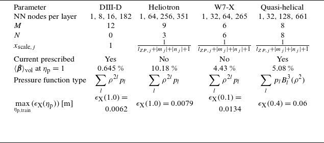


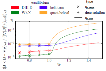


 Open access