

INTRODUCTION
With an ice coverage of 40 775 km2, the Himalaya-Karakoram region has one of the largest glacier coverages outside the Polar regions (Bolch and others, Reference Bolch2012; Frey and others, Reference Frey2014). Livelihood of a sizeable part of the population is dependent on glacier fed rivers that originate from The Himalaya. Recent investigations suggest that the majority of Himalayan glaciers are retreating due to climate change (Kulkarni and others, Reference Kulkarni, Rathore, Singh and Bahuguna2011; Kulkarni and Karyakarte, Reference Kulkarni and Karyakarte2014). Therefore, in order to assess their sustainability as well as future evolution, it is important to explore the relationship between glacier front fluctuations and climate change. A record of glacier mass balance is an important tool for such studies. However, owing to harsh climatic conditions and difficult terrain in this region, mass-balance investigations have been difficult and also are limited to few selected glaciers (Berthier and others, Reference Berthier2007). Apart from mass balance, topographic maps and glacier retreat records do give some insight into changes in glacier length and surface area, but the state of balance or imbalance with respect to local climate cannot be inferred (Oerlemans, Reference Oerlemans2001). In such a situation, numerical modelling of glacier flow can be a feasible alternative to in-situ measurements. Numerical flowline modelling has been successfully used for estimating past retreat as well as future evolution of glaciers located in different climatic conditions, around the world (Stroeven, Reference Stroeven1996; Oerlemans, Reference Oerlemans1997; Schmeits and Oerlemans, Reference Schmeits and Oerlemans1997; De Smedt and Pattyn, Reference De Smedt and Pattyn2003). Unfortunately, such flowline studies have not been carried out in the Indian Himalaya.
In this paper, we use a numerical flowline model to simulate the past retreat and future evolution of Chhota Shigri glacier, located in the Indian Himalaya. The glacier was considered for our analyses, mainly because it has been chosen as the benchmark glacier in the western Himalaya; is easily accessible; and most importantly, it is located in an area influenced by Indian monsoon in summer and mid-latitude westerlies in winter (Wagnon and others, Reference Wagnon2007). A wide accumulation area and a relatively narrow ablation zone renders the glacier sensitive to climate change. Also, among other Himalayan glaciers Chhota Shigri has one of the longest records of continuous in-situ mass-balance estimates spanning 2002–14 (Azam and others, Reference Azam2016).
STUDY AREA
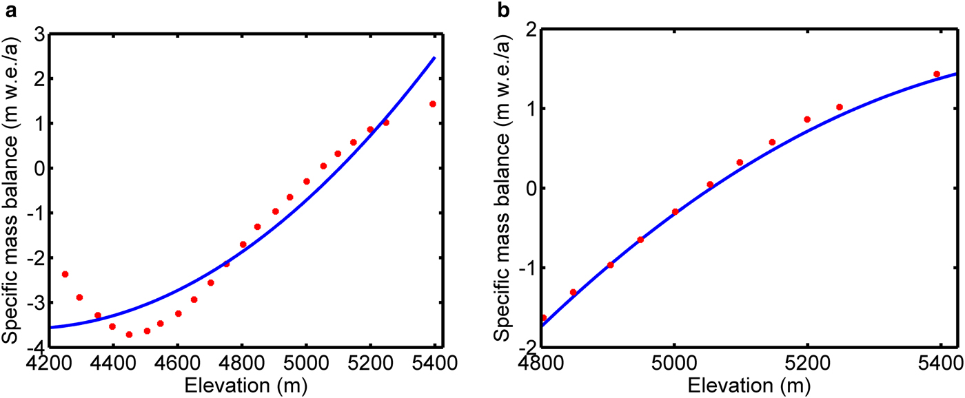
The Chhota Shigri glacier is located on the Chandra river basin in Himachal Pradesh (Fig. 1). The valley glacier is oriented north-south in ablation zone, and the accumulation zone is differently oriented. The glacier geometry is complex with three tributaries. The ice flow in the main trunk is mainly due to ice from the tributary (B) and the main trunk (A) (Wagnon and others, Reference Wagnon2007). The ice flow in the accumulation zone has contribution from four small cirques namely b1, b2, b3 and b4 (Fig. 1). Continuous mass-balance observations have been carried out on this glacier since 2002 by the glaciological method (Wagnon and others, Reference Wagnon2007; Azam and others, Reference Azam2016). The observed specific mass balance averaged over every altitudinal band of 50 m is shown as a function of altitude in Figure 2. The specific mass-balance ranges from 1.5 to −2.5 m w.e. a−1. Below an altitude of ~4400 m, the specific mass balance increases due to the presence of debris cover (Azam and others, Reference Azam2016). Further details regarding specific mass balance of Chhota Shigri glacier can be found in Wagnon and others (Reference Wagnon2007); Azam and others (Reference Azam2016). In addition, point surface velocity and ice thickness observations are available for the year 2004/05 (Tiwari and others, Reference Tiwari, Gupta and Arora2014). The snout position has been monitored from 1962 onwards (Ramanathan, Reference Ramanathan2011). Since 1995, the glacier has been constantly retreating. From 1972 till 2009, the glacier has retreated by 800–850 m (Kulkarni and others, Reference Kulkarni2007; Shruti, Reference Shruti2008). The other characteristics of the glacier are listed in Table 1.
Map of Chhota Shigri glacier showing the different tributaries, cirques considered for the analyses. A, B represents the main stream and the tributary, respectively. b1, b2, b3, b4 represent the cirques that contribute ice to both A and B. The cross sections where GPR measurements were available have been labelled as 1, 2 and 3. In the inset map of India, the location of Chhota Shigri glacier is shown as a red dot. The flowlines used in the analyses are shown as dotted red lines. The cross section is parameterized as a trapezium of base width w b, height H. k1, k2 represent the orientation of the valley walls. λ = (tan(k1) + tan(k2)).

(a) Mass balance of main stream of Chhota Shigri glacier for the period 2002–14 (Azam and others, Reference Azam2016). Red dots represent the observed data and blue represents the quadratic polynomial that has been used as a fit to the mass-balance curve (R 2 = 0.89). (b) Mass balance of tributary of the glacier. It is estimated by correcting the mass-balance profile in ‘(a)’ for altitude. Red dots represent the observed data and blue represents the quadratic polynomial that has been used as a fit to the mass-balance curve (R 2 = 0.98). The polynomial fits are used to force the model.
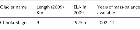
Chhota Shigri glacier mass-balance information
METHODOLOGY
Model used
The model used in this study is solely based on mass conservation, and it describes ice flow along the central flowline, assuming that a glacier cross section can be approximated as a trapezium. A detailed description of the model can be inferred from Oerlemans (Reference Oerlemans1997). For a given glacier cross section, mass conservation can be stated as
 $$\displaystyle{{\partial H} \over {\partial t}} = \displaystyle{{ - 1} \over {w_{\rm b} + \lambda H}}\displaystyle{\partial \over {\partial x}}((w_{\rm b} + 0.5\lambda H)UH) + B,$$
where H is local ice thickness (m), w b the width of cross-section's base (m), λ parametrizes the orientation of the side walls (Fig. 1), B is the specific mass balance (m w.e. a−1), t the time and U is vertically averaged mean cross-sectional velocity (m a−1). Since, the model is 1-D and neglects transverse gradients of velocity, vertically averaged and mean cross-sectional velocity are the same. U can be further expressed as
 $$U = f_k^{\rm 3} \left( {\,f_1 Y H^4 \left( {\displaystyle{{\partial h} \over {\partial x}}} \right)^2 \displaystyle{{\partial h} \over {\partial x}} + f_2 Y H^2 \left( {\displaystyle{{\partial h} \over {\partial x}}} \right)^2 \displaystyle{{\partial h} \over {\partial x}}} \right),$$
where $Y $
= (ρg)3, ρ is the ice density and is assumed to have a constant value of 900 kg m−3, g = 9.8 m s−2, f
1 and f
2 represent the deformation and sliding flow parameters and are assumed to be 1.9 × 10⁻²⁴ Pa−3 s−1 and 5.7 × 10⁻²⁰ Pa−3 m2 s−1, respectively (Budd and others, Reference Budd, Keage and Blundy1979), f
k is a correction factor that parametrizes the effects of lateral and longitudinal drag (Nye, Reference Nye1965; Adhikari and Marshall, Reference Adhikari and Marshall2011, Reference Adhikari and Marshall2012). However, lateral and longitudinal stresses seldom have an impact over decadal or century scale retreat as compared with mass balance (Oerlemans, Reference Oerlemans2001). In fact on repeating the analyses with f
k
= 1, the results were not different from those that were obtained by assuming f
k
to be a constant but not equal to one. This is probably because as compared with other model uncertainties and the rather simplistic treatment of ice flow, the effect of the correction factor is probably insignificant (Oerlemans, Reference Oerlemans2001); h is surface elevation (m), expressed as
$Y $
= (ρg)3, ρ is the ice density and is assumed to have a constant value of 900 kg m−3, g = 9.8 m s−2, f
1 and f
2 represent the deformation and sliding flow parameters and are assumed to be 1.9 × 10⁻²⁴ Pa−3 s−1 and 5.7 × 10⁻²⁰ Pa−3 m2 s−1, respectively (Budd and others, Reference Budd, Keage and Blundy1979), f
k is a correction factor that parametrizes the effects of lateral and longitudinal drag (Nye, Reference Nye1965; Adhikari and Marshall, Reference Adhikari and Marshall2011, Reference Adhikari and Marshall2012). However, lateral and longitudinal stresses seldom have an impact over decadal or century scale retreat as compared with mass balance (Oerlemans, Reference Oerlemans2001). In fact on repeating the analyses with f
k
= 1, the results were not different from those that were obtained by assuming f
k
to be a constant but not equal to one. This is probably because as compared with other model uncertainties and the rather simplistic treatment of ice flow, the effect of the correction factor is probably insignificant (Oerlemans, Reference Oerlemans2001); h is surface elevation (m), expressed as
 $$h = h_{\rm b} + H,$$
where h b is bed elevation (m). The model equation used in our analyses can be obtained by combining Eqns (1) and (2):
 $$\displaystyle{{\partial H} \over {\partial t}} = \displaystyle{{ - 1} \over {w_{\rm b} + \lambda H}}\displaystyle{\partial \over {\partial x}}\left( {D\displaystyle{{\partial h} \over {\partial x}}} \right) + B,$$
where D is defined as diffusivity (m2 a−1) and is expressed as:
 $$D = (w_{\rm b} + 0.5\lambda H)f_k ^3 \left( {\,f_1 Y H^5 \left( {\displaystyle{{\partial h} \over {\partial x}}} \right)^2 + f_2 Y H^3 \left( {\displaystyle{{\partial h} \over {\partial x}}} \right)^2} \right),$$
Specific mass-balance B can be further expressed as (Oerlemans, Reference Oerlemans2001)
 $$B(h,t) = B_{{\rm ref}} (h) + b(t) + \delta B,$$
where B ref is the reference specific mass-balance profile and is solely a function of h. B ref is obtained from glaciological records; b(t) represents the balance perturbations derived from proxies such as temperature, precipitation, tree rings etc. b(t) is purely a function of time and is applied irrespective of altitude; δB is a constant whose value is chosen such that the model produces equilibrium states that are very close to current glacier stands. δB is also applied irrespective of altitude.
Estimation of bed topography
Local ice thickness (H) is estimated using the relationship between surface velocity, slope and ice thickness (Paterson, Reference Paterson2010; Gantayat and others, Reference Gantayat, Kulkarni and Srinivasan2014)
 $$u_{\rm s} = u_{\rm b} + \displaystyle{{2A} \over {n + 1}}(\,f\,\rho gH{\rm sin}(\alpha ))^n, $$
where u s and u b represent the surface and basal velocities, respectively; u b is assumed to be 25% of u s, n = 3 is Glen's constant (Glen, Reference Glen1955), f is a correction factor that parametrizes lateral and longitudinal stress and it can be tuned using published estimates of observed ice thickness (Nye, Reference Nye1965; Adhikari and Marshall, Reference Adhikari and Marshall2011, Reference Adhikari and Marshall2012). For Chhota Shigri glacier, f was tuned at three cross sections namely 1, 2, 3 (Fig. 1) where observed ice thickness estimates were available (Azam and others, Reference Azam2012), A is Creep parameter = 3.2 × 10⁻²⁴ Pa−3 s−1 and sin(α) is the mean surface slope of every glacier area located between two altitudinal bands having 100 m difference in their respective elevations.
In this paper, for estimating H Eqn (7) was first solved along discrete points of manually digitized branchlines (e.g. Linsbauer and others, Reference Linsbauer, Paul and Haeberli2012), and the resulting ice thickness was spatially interpolated assuming zero ice thickness at the glacier margin. For interpolation, ANUDEM (Australian National University DEM) was used (Hutchinson, Reference Hutchinson1989). While digitizing individual branchlines, the following steps were taken: (a) a lateral spacing of 200–220 m was maintained between adjacent lines; (b) a minimum distance of 100–150 m was maintained between the branchlines and glacier margin; (c) the branchlines from a tributary were made to gradually merge with the branchlines from the main stream. Bed elevation was then estimated by subtracting the resulting ice thickness map from the local DEM. Lastly, the bed topography was smoothed using a 3-by-3 filter to remove small undulations. Details regarding the algorithm can be found in Farinotti and others (Reference Farinotti2017).
The initial bed elevation profile (h b) and initial base width (w b) were estimated from the bed topography estimated above. For estimating the value of f k (see Eqn (2)), values of f across cross sections 1, 2 and 3 (Fig. 1) were estimated by tuning modelled ice thickness in Eqn (7) with GPR estimates. The value of f k was assumed to be the mean of the above estimated values of f.
NUMERICAL IMPLEMENTATION
Equation (4) was solved numerically along the two central flowlines with a horizontal grid spacing of 100 m (Fig. 1). It was observed that two flowlines would be sufficient to parametrize the ice flow in the Chhota Shigri glacier complex (Fig. 1). A forward explicit finite-difference scheme was used for the analyses.
Addition of ice from cirques to main stream
The accumulation zone of the main stream is partly fed by 3 cirques and the accumulation zone of the tributary by 1 cirque (Fig. 1). Details regarding the bed geometry of the cirques were not known and due to their steep slopes, shallow ice approximation will not be applicable. Therefore, it was decided to estimate only the mass flux from the cirques at every time step. To do so the scheme suggested by Schmeits and Oerlemans (Reference Schmeits and Oerlemans1997) was used. First, the ice volume of the cirque at time t is calculated according to
 $$\displaystyle{{{\rm d}v} \over {{\rm d}t}} = \mathop \sum \limits_i a(h_i )b(h_i ) - \displaystyle{v \over {t{^\ast}}},$$
where v is the volume of the cirque at time t. Here a(hi) and b(h i) are the area and the mass balance of the elevation interval (100 m in this study) respectively, centred around h i; i is the number of the elevation band. The first term on the right represents the mass gain and the second term represents volume lost to the main stream/tributary. t* is defined as the characteristic timescale and has been introduced to take into account owing to the fact that mass flux due to ice flow from the cirques to the main stream/tributary may take several years. t* is defined as
 $$t{^\ast} = \displaystyle{{L{^\ast}} \over {U{^\ast}}},$$
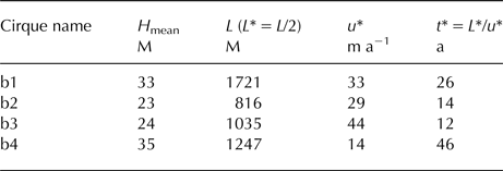
where L* and U* are defined as the characteristic length scale and velocity, respectively. L* is assumed to be half the cirque's length. U* depends on the mean ice thickness and mean surface slope of the basin. Therefore, t* varies from cirque to cirque. A list of t* for the 4 cirques has been given in Table 2. Therefore, at every time step Δt, an amount of ice volume equal to ((v/t*)Δt) is added from the cirques. The ice volume is then equally distributed over a certain number of grid points on the main stream/tributary (for numerical stability). This is then converted to respective ice thickness and is added at the respective gridpoints.
Estimated characteristic timescales of the four cirques
Addition of ice from tributary to main stream
The ice flux from the tributary to the main stream is estimated (Schmeits and Oerlemans, Reference Schmeits and Oerlemans1997) as follows:
 $$F = U(wH).$$
At every time step Δt, the flux between the last two gridpoints of the tributary was estimated and was assumed to be a good approximation of the ice flux that is added from the tributary to the main stream. Ice flux times Δt gives the volume that is added to the main stream. If the surface elevation of the tributary was more than that of the main stream, ice volume was added to the main stream. The volume is equally distributed across the nearest three grid points on the main stream (for numerical stability). The distributed volume is then converted into respective ice thickness, which is added to the main stream at the corresponding gridpoints.
Estimation of Δt (time step)
For solving Eqn (4) for a glacier with unit width, a critical time step of 0.01 a was estimated using the CFL condition (Smith, Reference Smith1978):
 $$\Delta t \le (\Delta x)^{\rm 2} /{\rm 4}D_{\rm a}, $$
where Δx is the horizontal grid spacing and D a is the average diffusivity. Finally, for the simulation of retreat of Chhota Shigri glacier (accounting for the variable width), a step of 0.001 a was chosen because lowering the time step further, did not affect the model results.
DATA USED AND MODEL INITIALIZATION
For solving Eqn (4), we need (a) two central flowlines representing ice flow along main trunk and tributary, (b) surface elevation profile along the flowlines, (c) initial bed elevation profile along the flowlines, (d) initial estimate of w b and λ, (e) reference mass-balance profiles, and (f) proxy data for simulating retreat.
The two central flowlines were manually digitized such that they were orthogonal to the surface elevation contours (Fig. 1). Surface elevation values required for the model were taken from the local ASTER DEM (downloaded freely from earthexplorer.usgs.gov/). To remove spatial bias, it was co-registered with one of the Landsat 8 images and was then smoothened using a 3-by-3 filter. The DEM obtained now was used in further analyses. The surface elevation values required for Eqn (1) were extracted from DEM using ArcMap 9.2. For estimating initial bed topography, ice thickness was estimated from surface velocities generated using 2 Landsat-8 PAN scenes (Table 3). Surface velocities were estimated using sub-pixel correlation (e.g. Leprince and others, Reference Leprince, Barbot, Ayoub and Avouac2007; Gantayat and others, Reference Gantayat, Kulkarni and Srinivasan2014). To tune the ice thickness model, we have published estimates of observed ice thickness across three cross profiles. These observations were taken during October 2009 (Azam and others, Reference Azam2012). While doing so we assumed that over a period of 5–6 years, the ice thickness and surface elevation values will not change drastically (>RMS error of the DEM). Mass-balance profile (2002–14) for the main stream was inferred from Azam and others (Reference Azam2016). The balance profile of the tributary was derived by correcting the main stream's mass-balance profile for altitude (Fig. 2). B ref for both main stream and tributary was estimated by fitting a second-order polynomial through the data points (Figs 2a, b). For simulating retreat, annual mean temperatures and annual and seasonal accumulated precipitation (since, 1876) from the meteorological observatory at Shimla has been taken. The observatory is located at 31.1048° N, 77.1734° E, at an elevation of 2202 m and is maintained by the Indian Meteorological Department (IMD) (Fig. 1).
Details of satellite imagery used, resolution of the velocity map

Using the above data, zero ice volume as the initial condition, and the flow parameters (f 1 and f 2) specified above, the model (Eqn (4)) was run by setting δB = 0. δB was then adjusted in order to simulate a steady-state glacier having the same length as that of Chhota Shigri in 2009 (9 km) (Wagnon and others, Reference Wagnon2007). The flow parameters and the bed geometry were adjusted till the RMS difference between simulated and observed surface elevation in 2009 was minimum as well as until the area-altitude distribution of the simulated glacier matched with that derived from the DEM within acceptable limits (<0.1 km2 in our case) (e.g. Oerlemans, Reference Oerlemans2001). While adjusting the bed, care was taken to ensure that the geometry of the cross sections where ice thickness was modelled using GPR measurements was not altered (Fig. 1). While adjusting the flow parameters, due to lack of field estimates of f 1 and f 2, it was decided to keep the ratio f 1 :f 2 constant at all times. It was observed that along with the above specified modifications, when δB was assigned a value of 0.03 and 0.06 m w.e. a−1 for A and B, a steady-state glacier with length corresponding to that in 2009 was simulated. Such an approach for tuning flow parameters and bed geometry has been used in the past (e.g. Adhikari and Huybrechts, Reference Adhikari and Huybrechts2009). Instead of tuning the flow and bed parameters by simulating a steady state, we also tried to tune the bed and flow parameters by minimizing the RMS difference between observed and a simulated dis-equilibrium 2009 surface elevation values. The dis-equilibrium state was simulated by forcing the model with a constant balance perturbation of 0.08 m w.e. a−1 from AD1000–1875 and b(t) for the period 1876–2009. The results obtained from both the kinds of tuning were very similar.
Finally, the adjusted bed along with the adjusted flow parameters was used in subsequent analyses.
RESULTS
Estimation of bed topography
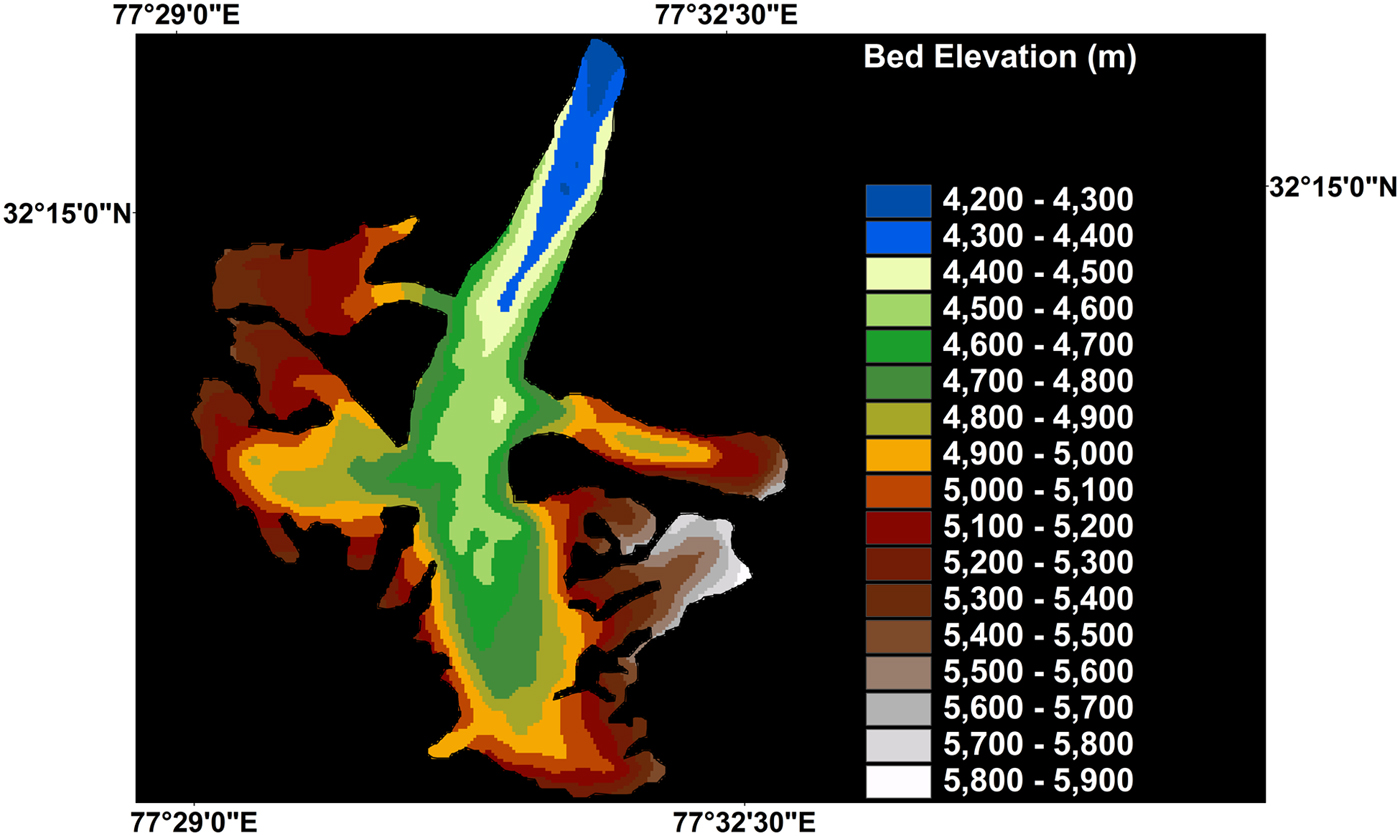
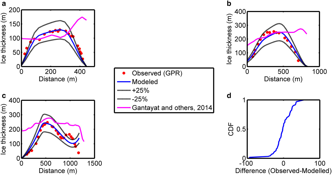
The bed topography of Chhota Shigri glacier is shown in Figure 3. The bed elevation varies from ~4200 to 4500 m in the ablation zone and ~5000–5900 m in the accumulation zone. The bed elevations along three cross sections were validated with GPR measurements (Figs 1, 4). The mean and standard deviation of the uncertainty is ~17 and ~16 m, respectively. The empirical Cumulative Distribution Function (CDF) of the uncertainty shows that ~74% of observed ice thickness values were within ±25% uncertainty in the corresponding modelled ice thickness profiles. A comparison with the cross-sections modelled using Gantayat and others (Reference Gantayat, Kulkarni and Srinivasan2014) also shows that the proposed modification using branchlines gives better results.
Modelled bed elevation of Chhota Sigri ranged from ~4200 to 4300 m near the snout and ~4400 to 4450 m elsewhere along the main trunk. For running the model, the bed elevations along the central flowline was considered as input.
(a–c) Validation of modelled ice thickness profiles across three cross sections with GPR derived ice thickness (Azam and others, Reference Azam2012). A model inter-comparison was done with the ice thickness profiles estimated according to Gantayat and others (Reference Gantayat, Kulkarni and Srinivasan2014). (d) The empirical cumulative probability distribution function (CDF) of the difference in observed and modelled ice thickness at three cross sections.
Estimation of response time
When the model is run with the adjusted parameters, it takes ~320 years to produce a steady-state glacier. The steady-state glacier is then subjected to various balance perturbations after 500 years of model run and the subsequent response of the glacier length is shown in Figure 5.
Response of the steady-state glacier length to different balance perturbations. The response times for positive perturbations are slightly lesser than that for negative perturbations. Average length response time is ~67 years.
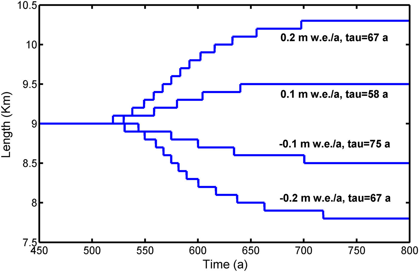
The length response time is defined as the time period required to reach (1 × 10⁻¹) of the final response after a stepwise perturbation in climate. The response times were 75 and 67 years for balance perturbations of −0.1 and −0.2 m w.e. a−1, respectively. For positive perturbations of 0.1, 0.2 m w.e. a−1 the response times were 58 and 67 years, respectively. The response times for positive perturbations is slightly less than that for negative perturbations. This is because during retreat the glacier front enters a bed with a relatively smaller slope as compared with that during advance. Similarly, the volume response times for the same set of balance perturbations were 35, 36 years for positive perturbations (0.1, 0.2 m w.e. a−1) and 38, 40 years for negative perturbations (−0.1, −0.2 m w.e. a−1). Therefore, the average volume response time leads the average length response time by ~30 years. The volume response time was also estimated according to Johannesson and others (Reference Johannesson, Raymond and Waddington1989),
 $$\tau _{{\rm rvh}} = H \times / \vert {\rm B}_{{\rm term}} \vert, $$
where τ rvh is the volume response time, H* is mean ice thickness and B term is the specific balance at the terminus. τ rvh for Chhota Shigri is ~33 years.
The glacier carries memory of the past climate for a time period equal to one or two times the response time (Oerlemans, Reference Oerlemans2001). Therefore, the length response time gives an estimate of how far in time one must run the model to correctly simulate the historical retreat.
Simulation of retreat
The observed retreat record for Chhota Shigri glacier is rather short (48 years). The large response time of the glacier suggests that the model run should start well before the retreat record. In addition, the mass-balance observations span the period 2002–14, which is also quite small. Therefore, in order to reconstruct the mass-balance history over the past two centuries, we used climate proxies such as temperature and precipitation. We decided to adopt a temperature index like approach (e.g. Zuo and Oerlemans, Reference Zuo and Oerlemans1997; Adhikari and Huybrechts, Reference Adhikari and Huybrechts2009).
For reconstructing the past mass-balance history, annual mean temperature and annual and seasonal accumulated precipitation (1876–2009) from the Meteorological station at Shimla, Himachal Pradesh, were used (Fig. 6a). The major reason behind chosing this station is its long records of temperature and precipitation that span over 134 years, which is also roughly double the average length response time and for a successful retreat simulation, the model run must start from a time that is twice the response time (Oerlemans, Reference Oerlemans1997; Adhikari and Huybrechts, Reference Adhikari and Huybrechts2009). The other nearby meteorlogical stations have much shorter records.
(a) Meteorological data from Shimla (1876–2009) (a) Annual mean temperature anomalies, (b) Annual mean precipitation anomalies by ratio, (c) Seasonal accumulated precipitation anomalies by ratio. (b) Balance perturbations derived from (a) annual mean temperature anomalies, (b) annual mean temperature and annual mean precipitation anomalies, (c) Annual mean temperature and seasonal mean precipitation anomalies.

Before carrying out further analysis, we chose to fill in the data gaps. For that we estimated the average of five data points prior to the gap and five points later. We assumed that the average of the two averages is a good estimation for the void. The annual mean temperature showed more correlation with the annual mean mass balance (R = 0.5) than that between annual accumulated precipitation and annual mean mass balance (R = 0.4). Due to the limited years of mass-balance measurements (2002–14), a proper forcing function had to be established for simulating retreat. Assuming a linear relationship between past balance perturbations, and temperature and precipitation (e.g. Adhikari and Huybrechts, Reference Adhikari and Huybrechts2009), b(t) is expressed as:
 $$b(t) = \beta (\Delta T + \mu _{\rm 1} ) + \theta (\Delta P + \mu _{\rm 2} )$$
where ΔT, ΔP represent temperature and precipitation anomalies by ratio, respectively. Precipitation anomalies by ratio were obtained by dividing annual/seasonal mean precipitation by their corresponding mean for the period 1876–2009. In our analyses, anomalies were estimated considering 1876–2009 as the base period. β and θ are defined as the mass-balance sensitivity to temperature (m w.e./°C) and precipitation sensitivity (m w.e. m−1) respectively. Their values are unique for each glacier (Adhikari and Huybrechts, Reference Adhikari and Huybrechts2009); μ 1 and μ 2 serve as tuning parameters. Their values are fixed by trial and error so as to get minimum RMS difference between observed and simulated snout positions.
The maximum difference between the observed ELAs as well as the difference between the corresponding annual mass balance was estimated (from 2002 to 2014) from Azam and others (Reference Azam2016). Assuming a vertical lapse rate of −6.5°C km−1, the value of β was estimated to be −0.7 m w.e./°C. The estimated value of β is well within the range of (−0.52 to −1), which was estimated by Azam and others (Reference Azam2016) using a degree day model. Interestingly, the value of −0.7 m w.e./°C was estimated at the ELA by Azam and others (Reference Azam2016). The lapse rate is likely to vary seasonally in a complex terrain like the Himalaya. But since the model is forced with mass-balance changes averaged over a year, a constant annual mean value for the lapse rate was assumed, which has also been used previously (e.g. Adhikari and Huybrechts, Reference Adhikari and Huybrechts2009).
The winter accumulated precipitation recorded at base camp shows a maximum difference of 290 mm w.e. for the years 2009/10 and 2012/13 (Azam and others, Reference Azam2016). For estimating θ, the change in annual mean mass balance for the corresponding years was estimated. θ was estimated to be 0.003 m w.e. mm−1. In order to get minimum RMS error between observed and simulated lengths, the values of μ 1 and μ 2 were estimated to be 0.08 K and 0.07, respectively.
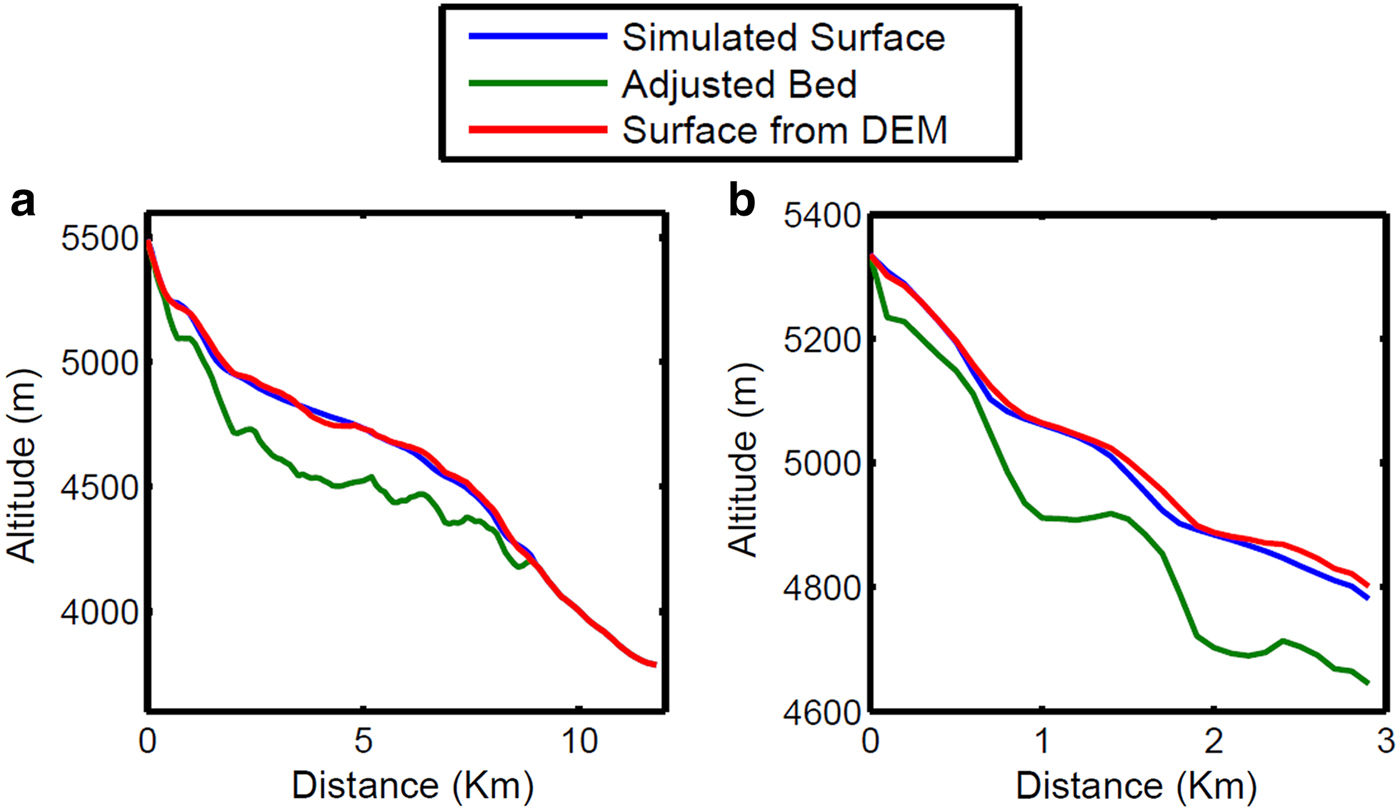
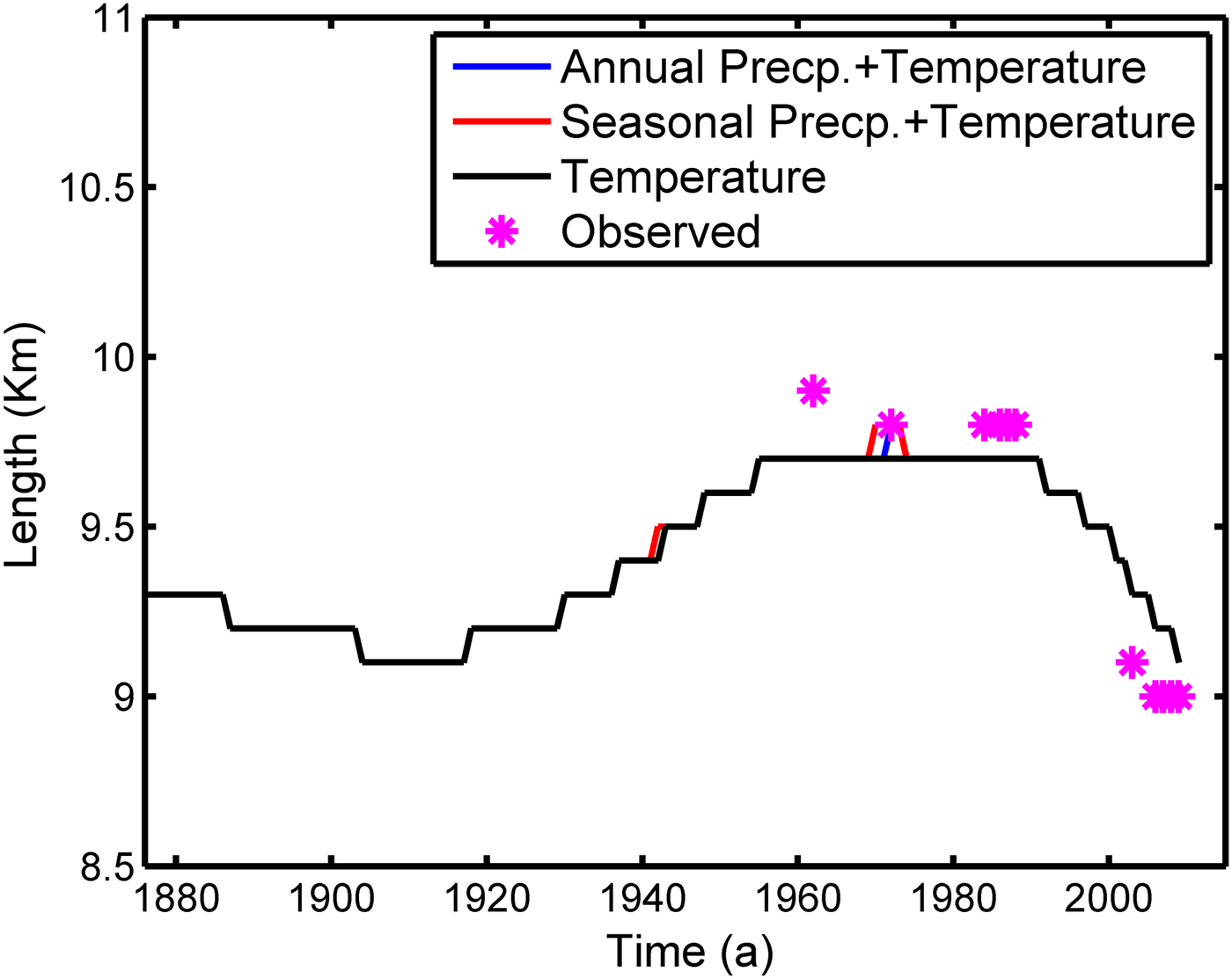
Our simulation of historic retreat started at the year AD 1000 with zero ice volume as the initial condition and δB was set to zero for both the main stream as well as the tributary. Due to non-availability of meteorological data prior to 1876, we decided to use the period from 1000 to 1875 as a tuning period. From 1876 onwards, the model was forced with b(t) as shown in Figure 6b. A comparison of the simulated and observed surface elevations of the main stream shows good correlation with an RMS difference of ~16 m (Fig. 7). The simulated and observed surface elevation profiles of the tributary also match quite well with an RMS error of ~15 m (Fig. 7). The simulated glacier length fluctuations also match with that observed with an RMS error of ~150 m (Fig. 8). The simulated glacier in 2009 is longer than the observed length by ~100 m.
(a) Comparison of simulated and observed surface elevation of A (main stream). The RMS error is ~16 m. (b) Comparison of simulated and observed surface elevation of B (tributary). The RMS error is ~15 m. The adjusted bed profile has been shown as a green line.
Glacier length fluctuations due to mass-balance changes derived from climate forcing (Fig. 6b). The ‘*’ represent the observed front positions. The constant length prior to 1876 is due to the fact that a constant balance perturbation of 0.08 m.w.e. a−1 was used. The RMS difference between observed and simulated glacier lengths is ~150 m.
DISCUSSIONS
Characteristics of the simulated 2009 glacier stand
The simulated driving stress is shown in Figure 9. Except for a small region in the altitude band between ~4900 and 5000 m, the driving stress is in the range 100–200 KPa, which is typically the range in glacier ice. The very high value of the stress ~250 KPa in the altitudinal range 4900–5000 m is due to the presence of very steep slopes in that part of the glacier bed.
(a) Simulated mean velocity field during the year 2009. The observed surface velocities during 2004/05 have been represented as ‘*’. (b) Simulated driving stress during the year 2009.
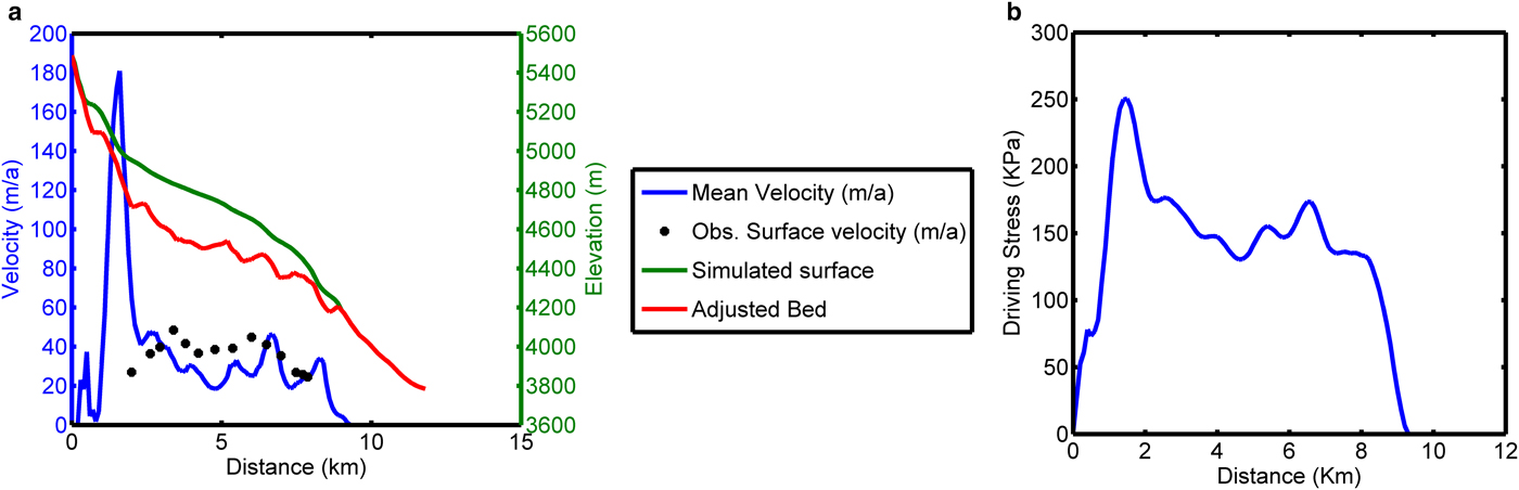
The simulated mean velocity field is also shown in Figure 9. The mean velocity ranged from ~180 to 10 m a−1. As ice is lost, the velocity vanishes at the top and glacier's snout. Very high velocity is again found in that altitudinal band of 4900–5000 m due to very high bed slope. The velocity peaks near the two icefalls at ~6.5 and ~8 km from the glacier top. High bed slopes result in less ice thickness, thus increasing the sliding component of the mean velocity (Figs 9, 10). A direct comparison of simulated mean velocity profile and that observed is difficult because the field measurements do not allow a calculation of the mass flux through a glacier cross section averaged over several years, which is what the model simulates (Oerlemans, Reference Oerlemans1997). However, a comparison of surface velocities for the year 2004/05 (Azam and others, Reference Azam2012) with mean velocity simulated in 2009 shows that the simulated mean velocity is typically in the range 0.7–1 times the surface velocities everywhere, except in the altitudinal band of 4900–5000 m.
Simulated mean, deformation and sliding velocity profiles in 2009.
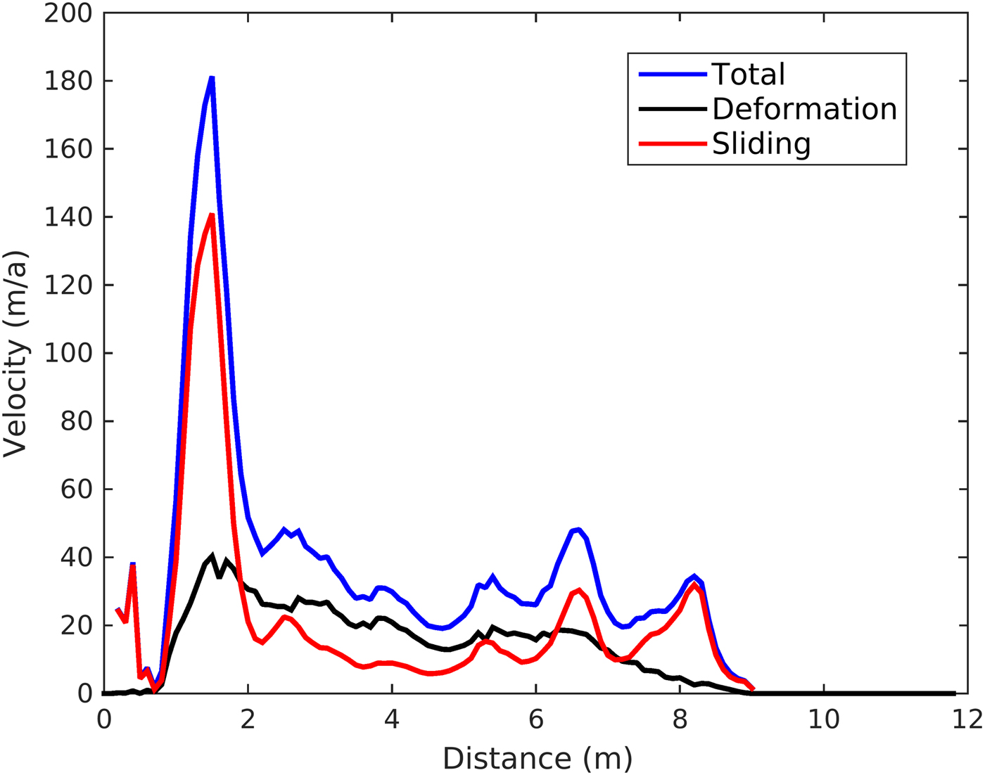
Steep bed slopes indicate presence of icefall in the altitudinal band ~4900–5000. Here, the model over-estimates the velocity. This is due to the simplistic manner in which U has been formulated in Eqn (2). In reality sliding occurs possibly due to the subglacial lubrication by meltwater that is generally absent in the icefalls. As a result, the effect of higher order stresses on sliding becomes dominant (Adhikari and Marshall, Reference Adhikari and Marshall2013). Another reason could be due that the Chhota Shigri glacier is variously oriented in the accumulation zone (Wagnon and others, Reference Wagnon2007), the flowline approximation of the model might not hold true. However, this does not affect the simulation of frontal variation probably because that is mostly governed by dynamics in the ablation area (De Smedt and Pattyn, Reference De Smedt and Pattyn2003).
Analysis of past retreat and future projections
The simulated glacier length increased from 1900 to 1950 and remained constant until ~1991. From 1992 onwards, there has been a continuous retreat; the advance resulted due to a relatively cool period from ~1900 to 1960 (Figs 6b, 8). The retreat after 1995 seems to be quite rapid when compared with the rate of advance during the period 1900–50. From 1972 to 2006, the modelled retreat was ~700 m, which is quite close to 850 m, a value that was estimated using satellite imagery (Shruti, Reference Shruti2008). The fast retreat can be attributed to two factors: (a) rise in temperature; (b) presence of steep bed below an altitude of 4200 m. The simulation also suggests that from ~1972 to 1992, the glacier was in a steady state.
We also tried to determine the dominant climate proxy responsible for retreat. Two experiments were carried out. In the first one, we estimated retreat using only temperature anomalies. In the second experiment, retreat was estimated using both temperature and precipitation anomalies. The results show that precipitation hardly influences the glacier length variations (Fig. 8). Thus, we conclude that historical length variations of Chhota Shigri glacier are mostly influenced by temperature and not precipitation.
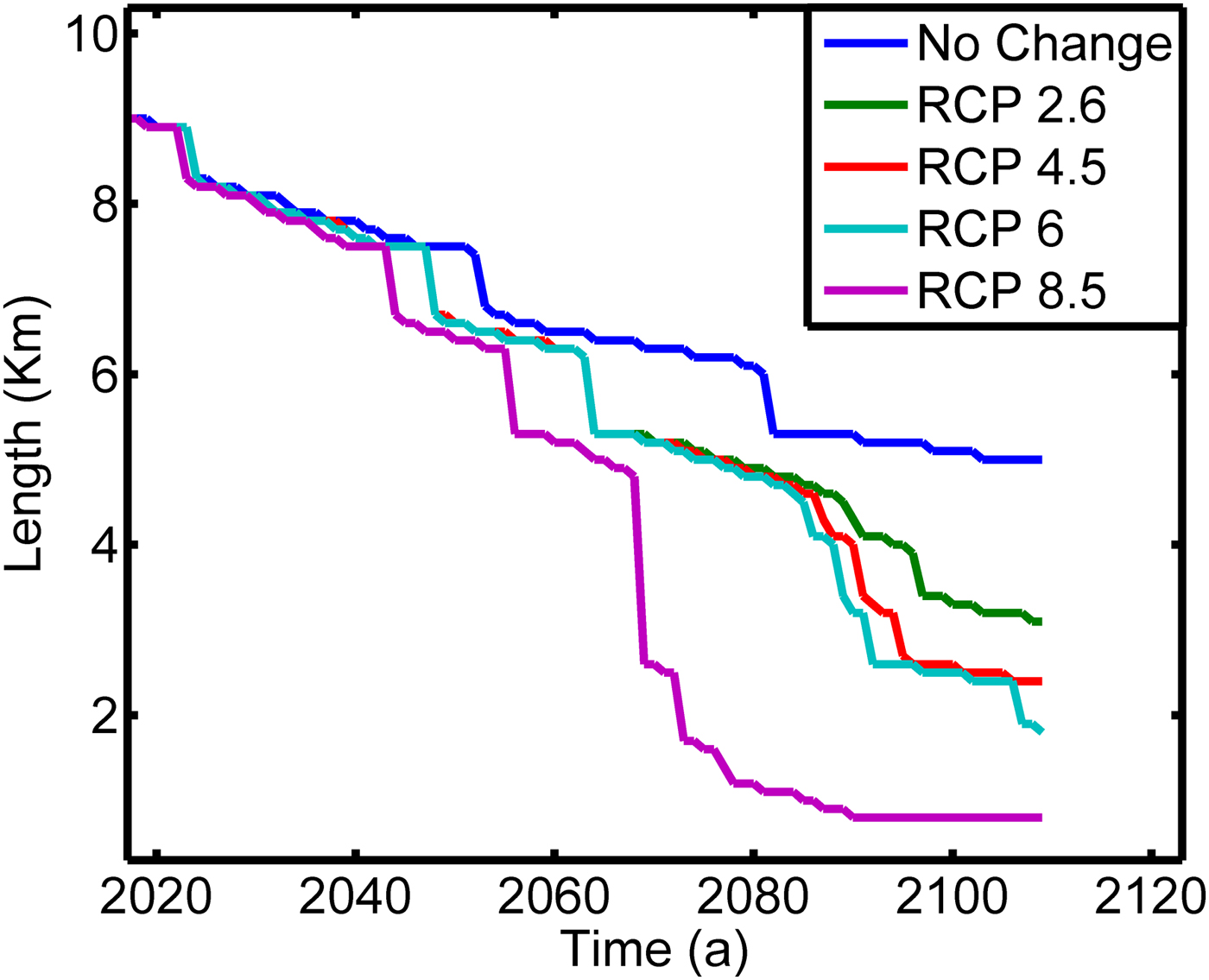
After having successfully simulated the historic retreat, four different climatic scenarios under constant precipitation were analysed for predicting the glacier's future evolution. These climatic scenarios have been named as RCP 2.6, RCP 4.5, RCP 6 and RCP 8.6. They predict a temperature rise of 2.36, 3.49, 3.68 and 5.51°C with respect to 1860–1990 mean, respectively, in the Western Himalaya Karakorm over the next 100 years. Details regarding the scenarios can be inferred from Chaturvedi and others (Reference Chaturvedi, Kulkarni, Karyakarte, Joshi and Bala2014).
The trend of the temperature rise was estimated and was used for model runs after 2009. The results are shown in Figure 11. If the mean temperature for the period 1990–2009 was assumed to be the mean temperature after 2009, the glacier can be expected to retreat by ~4 km and lose 73% of 2009 volume by AD 2109. Under RCP 2.6 and 4.5 situations, the glacier is expected to retreat by ~6 and 6.6 km as well as lose 92% and 97% of its 2009 volume, respectively. Under RCP 6 conditions, the glacier is expected to retreat by ~7 km. Under RCP 8.5 conditions, a steep decrease in the glacier length is to be expected after ~2090 because the glacier breaks into fragments.
Glacier length changes under different climatic scenarios.
CONCLUSIONS
In this study, we present a numerical ice flow model that was used to simulate the historical retreat and future evolution of Chhota Shigri glacier. The simulation was successful with an RMS error of 150 m between simulated and observed snout positions. This study shows that flowline models can be used to understand the relationship between Himalayan glaciers and climate change. The simulations show that within the next 100 years, the glacier is expected to retreat further by between ~6 and 6.6 km for a 2.36 and 3.49 K rise in temperature, respectively. If the annual mean temperature after 2009 is same as the mean temperature for 1990–2009, the glacier retreats by ~5 km. The glacier ceases to exist by AD 2109 in case of a temperature rise of 5.5 K.
ACKNOWLEDGEMENTS
We thank Divecha Centre for Climate Change for providing the necessary laboratory resources that were required for this study. We also thank USGS for its free data policy, allowing us to use Landsat 8 Pan imagery.


 Open access