

Introduction
Over the past decade, driven by growing interest in global warming, studies of past natural proxy data – indirect indicators of climate and weather that are independent of man-made sourcesFootnote 1 – have increased drastically and have seen significant advancements in methodology, modelling, and both geographical and temporal scales (Consortium et al., Reference Consortium2017; e.g., Warren et al., Reference Warren, Bartlome, Wellinger, Franke, Hand, Brönnimann and Huhtamaa2024). This breakthrough, together with the meticulous work of climate historians, has consistently enhanced our understanding of past climate conditions and their effects on pre-industrial societies. The increased precision and resolution of proxy data have enabled a growing number of scholars to quantitatively explore the impact of climate and weather conditions on economic development, particularly in agriculture, the dominant economic sector before the Industrial Revolution (Cook and Wolkovich, Reference Cook and Wolkovich2016; e.g., Ljungqvist et al., Reference Ljungqvist, Thejll, Christiansen, Seim, Hartl and Esper2022; Pei et al., Reference Pei, Zhang, Li and Lee2015, Reference Pei, Zhang, Lee and Li2016). However, despite the increase in both quality and quantity of analysis on the topic, empirically establishing the influence of weather conditions on past agriculture practices has remained largely elusive (Erdkamp, Reference Erdkamp2021b; Ljungqvist et al., Reference Ljungqvist, Seim and Huhtamaa2021). On the one hand, some studies have failed to analyse the impact of climate on agriculture (at least statistically speaking), while others, although recognizing it, have found very heterogeneous and, not seldom, controversial results. This paradox is noteworthy because studies of contemporary agroecosystems clearly show that biophysical processes are strongly influenced by climatic factors such as temperature, rainfall, and atmospheric CO2 concentration (Agnolucci and De Lipsis, Reference Agnolucci and De Lipsis2020; Olesen and Bindi, Reference Olesen and Bindi2002; Uleberg et al., Reference Uleberg, Hanssen-Bauer, van Oort and Dalmannsdottir2014).
The difficulty in quantitatively analysing the relationship between weather conditions and agriculture in the pre-industrial world stems from various causes at different levels, both theoretical and methodological. The latter concerns the reliability of climate proxies, coupled with well-known challenges associated with historical agricultural data, while the former involves issues related to quantitatively analysing (i.e., model specification) the relationships between weather conditions and agricultural outcomes (cf. Van Bavel et al., Reference Van Bavel, Curtis, Hannaford, Moatsos, Roosen and Soens2019).
The reliability of paleoclimatic data, especially the earliest reconstructions or those from the most ancient times (i.e., the First Millennia reconstruction), was derived from theoretical meteorological models based on sparse proxies characterized by time-uncertain and small samples of observations, usually confined to specific and limited areas (e.g., Büntgen et al., Reference Büntgen, Tegel, Nicolussi, McCormick, Frank, Trouet, Kaplan, Herzig, Heussner and Wanner2011; Mann et al., Reference Mann, Bradley and Hughes1999). This has limited (and currently limits) the capacity to reconstruct reliable time series, especially to realistically represent large-area (national or continental scale) climate shifts (Anchukaitis and Smerdon, Reference Anchukaitis and Smerdon2022; Erdkamp, Reference Erdkamp2021a). Moreover, despite significant improvements, most of these time series reconstructions exhibit very low resolution; few provide more than annual data, which are, in addition, typically filtered to remove long-term trends. Although having annual data for historical studies is quite an achievement, it is often inadequate for accurate statistical analysis that effectively captures short-term impacts, such as the effect of weather conditions on harvests, which ideally requires monthly data or even higher levels of chronological resolution (Contreras et al., Reference Contreras, Guiot, Suarez and Kirman2018; Erdkamp, Reference Erdkamp2021b). Indeed, studies in contemporary wheat production have shown that neither high temperatures nor water deficits have a uniform effect on wheat yield; the impact strongly depends on the affected growth phase, which, by definition, is marked at a more granular frequency (Lawlor and Mitchell, Reference Lawlor and Mitchell2000; Li et al., Reference Li, Dong, Qiao, Liu and Zhang2010; Ventrella et al., Reference Ventrella, Charfeddine, Moriondo, Rinaldi and Bindi2012).
On the other hand, the model specifications (and assumptions behind them) adopted in these quantitative analyses have not rarely suffered from a lack of completeness and coherence. For example, these studies have typically devoted less attention to accounting for heterogeneity in plant types or geographic locations, which are crucial for accurately assessing the impact of climate on agriculture without bias (Heinrich and Hansen, Reference Heinrich and Hansen2021; Ongaro et al., Reference Ongaro, Prosperi and Ronsijn2024). Indeed, most empirical studies encompass an aggregate variety of crops (e.g., wheat, rye, spelt, etc.) across diverse and often disparate locations (such as hilly terrain, plains, mountains, coastal zones, etc.), regardless of the potential bias that such misspecifications may introduce in the results.Footnote 2
Last but not least, the model specifications adopted in these quantitative studies, especially macro-level ones, have generally been flawed by omitted variable issues and unmodeled expectations. This is mainly due to underestimating the role of societies in mitigating climate impacts, assuming a straightforward and one-way influence from weather conditions to agricultural outcomes. Factors such as human agency in weather mitigation, technology advances, social-political breakthroughs, farmers’ strategic decisions, and market forces have often been overlooked or oversimplified. However, this is not totally unexpected, given that macro studies, which typically cover the entirety of Europe and span several centuries, make it challenging to account for nuanced geographical differences and socio-political historical boundaries, and even more challenging to include in model specifications.
In this paper, we attempt to overcome these limitations starting from the bottom, fundamentally empirically ‘micro-founding’ the relationship between weather, agriculture, and human agency. First, we focus exclusively on a specific and well-defined spatio-temporal subject, Tuscany in central Italy from the 16th to 17th century, to minimize confounding factors related to comparing geographically and environmentally heterogeneous locations and/or divergent technological and socio-political frameworks. Specifically, we choose two locations in that region that offer sufficient data for statistical analysis: Florence and Siena and their surrounding area. Second, we concentrate solely on one category of crop, durum wheat. Third, we implement a full-specification model capable of accounting not only for the relationship between weather and agriculture but also for how human actions can mitigate or aggravate the impact of weather on agriculture. Specifically, we analyse the relationship between temperature, rainfall, and harvest alongside the endogenous relationship between yields and prices, employing an Autoregressive Distributed Lag (ARDL) model (Bai and Kung, Reference Bai and Kung2011; Jorgenson, Reference Jorgenson1966). This model is designed to capture not only the direct response of yields to external weather shocks but also the influence of additional channels rooted in production function factors and market dynamics, under the assumption of limited technological advancement in agricultural productivity (Malanima et al., Reference Malanima and Breschi2002). Specifically, the model specification controls for the roles of land, labour, and capital, as well as for the speculative behaviour of landowners driven by price expectations (i.e., hoarding practices).
Our empirical estimates indicate that, on average, increases in spring and summer temperature and rainfall improved harvests in both Florence and Siena during the 16th and 17th centuries, consistent with the idea that warmer and wetter growing seasons generally enhance plant growth. However, their impact needs to be contextualized alongside historical, geographical, and economic factors. Indeed, the mode of production in pre-industrial times, including soil conditions, capital-labour ratios, and broadly defined technological conditions, remains the most significant factor in explaining the variability in harvest yields. Additionally, the impact of short-term weather conditions appears amplified in the Siena region due to a combination of geographical features and historical developments. First, in the Sienese hinterland, unlike Florence, the morphology of the territory – characterized by predominantly clay hills (i.e., badlands) – makes extreme weather conditions, especially excessive rainfall, particularly detrimental (Calzolari et al., Reference Calzolari, Torri, Del Sette, Maccherini and Bryan1996; Ginatempo et al., Reference Ginatempo1988; Torri et al., Reference Torri, Rossi, Brogi, Marignani, Bacaro, Santi, Tordoni, Amici and Maccherini2018). Second, this heightened vulnerability in the Siena region, combined with a comparatively less effective annona system, leads to greater price volatility, creating a more favourable environment for the speculative behaviour of market-oriented landowners, which further exacerbates the negative effects of weather on the wheat market.
Our study hence presents a double contribution, one more specific and one more general. At the more specific level, we shed light on the relationship between weather conditions and agriculture in early modern Tuscany. On a more general level, this contribution highlights the importance of adopting a more comprehensive model specification to avoid assuming a simplistic and unidirectional link between weather and agricultural outcomes. Unlike most other studies on the topic, we found a strong interconnection between the exogenous effects of weather and the endogenous dynamics of societies in explaining agricultural performance. Specifically, production function capabilities can shrink (or expand) the range of optimal values, thereby amplifying (or reducing) the negative effects of weather. Meanwhile, competitive and integrated markets, when supported by countercyclical institutions – the annona system – can mitigate these effects, preventing the emergence of speculative behaviour and ensuring more stable markets.
The paper is organized as follows. In the second section, we provide a review of the literature, emphasizing both the relationship between weather and agricultural output and the associated methodological challenges. The third section outlines the economic history of Tuscany during the 16th and 17th centuries, offering the historical context necessary to interpret our empirical findings. In the fourth section, we present our data and model specification. The fifth section presents our estimates. In the sixth section, we conduct an in-depth discussion of our results. Finally, the seventh section offers our concluding remarks.
Background, challenges, and contributions
Background
The impact of climate on past societies, and particularly on their collapse, has long fascinated scholars from various disciplines, with historians and physical scientists playing a prominent role. The growing relevance of global warming in recent decades has further fuelled this field of inquiry, leading to a proliferation of climate-driven studies. In this context, climate has increasingly been invoked to explain a wide range of historical and socio-economic phenomena, from the emergence of the First Agricultural Revolution (Matranga, Reference Matranga2024) to the collapse of Late Bronze Age societies (Cline, Reference Cline2021), the rise and fall of Rome (Harper, Reference Harper2017), and the role of the early Little Ice Age in the breakdown of the Middle Ages (Parker, Reference Parker2013). However, although fascinating and stimulating in many ways, this all-encompassing use of climate as an explanandum for historical events has its pitfalls, often raising the problem of climate determinism (Hulme, Reference Hulme2011).
The proliferation of such ultra-long-run and geographically broad climate-determinist narratives has, in turn, prompted a response from scholars working in more specific fields, including economic historians. Indeed, a growing number of studies have started to quantitatively investigate the short-term impact of weather conditions (i.e., annual rainfall and temperatures) on agricultural productivity of grain, especially regarding the European early modern period, where both paleoclimatic and economic data on agriculture are more readily available (Campbell, Reference Campbell2010; Cook and Wolkovich, Reference Cook and Wolkovich2016; e.g., Ljungqvist et al., Reference Ljungqvist, Thejll, Christiansen, Seim, Hartl and Esper2022; Pei et al., Reference Pei, Zhang, Li and Lee2015, Reference Pei, Zhang, Lee and Li2016). However, despite a general consensus that weather conditions should exert a considerable impact on agriculture, the mechanisms by which this impact works – and its magnitude – remain largely controversial, particularly concerning the relationship between precipitation, temperature, and harvest, which is highly affected by spatio-temporal variations (Erdkamp, Reference Erdkamp2021b; Ljungqvist et al., Reference Ljungqvist, Seim and Huhtamaa2021).
A crucial part of this debate relates to the causal link by which temperature and sunlight affect the crop season, specifically its duration. In the case of wheat, the crop season is composed of four developmental stages (Chourghal et al., Reference Chourghal, Lhomme, Huard and Aidaoui2016): (1) initial stage (germination and seedling growth); (2) development stage (tillering); (3) mid-season stage (stem elongation); and (4) late development stage (anthesis and grain filling). In the Mediterranean region, this entire growth cycle averaged 216 days in the year 2000, with a variance of 33 days (Saadi et al., Reference Saadi, Todorovic, Tanasijevic, Pereira, Pizzigalli and Lionello2015). This variance is primarily driven by temperature and sunlight: higher temperatures tend to accelerate crop maturation, while lower temperatures slow it down, thereby shortening or lengthening the growing season. Variations in the length of the crop season can have both positive and negative effects on agricultural productivity. On the one hand, a shorter season allows crops to mature faster, helping them avoid the adverse effects of Mediterranean hot and dry late springs and summers, such as drought and heat stress (Ventrella et al., Reference Ventrella, Charfeddine, Moriondo, Rinaldi and Bindi2012). Additionally, a shorter season gives farmers more flexibility in managing sowing schedules – an essential adaptation strategy in pre-industrial times for coping with climate variability. On the other hand, some scholars argue that a reduced growing period may lead to lower biomass accumulation, which in turn can negatively affect harvest yields (Heinrich and Hansen, Reference Heinrich and Hansen2021; Saadi et al., Reference Saadi, Todorovic, Tanasijevic, Pereira, Pizzigalli and Lionello2015).
At different latitudes, such as in Central and Northern Europe and high-altitude regions, the relationship between temperature and agricultural productivity appears more straightforward. Macrogeographical studies have found a general correlation between higher temperatures and increased productivity in these areas (Barriendos, Reference Barriendos, Behringer, Lehmann and Pfister2005; Huhtamaa, Reference Huhtamaa2018; Pribyl, Reference Pribyl2017). This is because, in cooler regions, higher temperatures can shorten the crop season, reducing the risks associated with wet springs and cold summers. These conditions, especially in northern and high-altitude areas, could lead to freezing, which poses a significant threat to crop survival and yields (Aguado and Burt, Reference Aguado and Burt2007; Ljungqvist et al., Reference Ljungqvist, Thejll, Christiansen, Seim, Hartl and Esper2022; Malanima, Reference Malanima2014). However, other researchers contend that warmer temperatures do not inherently lead to improved agricultural performance at higher altitudes (Erdkamp, Reference Erdkamp2021b; Heinrich and Hansen, Reference Heinrich and Hansen2021). In addition to the effects of shortening (or lengthening) the growing season, another critical aspect of the debate centres on the specific role of ‘plants’ in the temperature-productivity relationship. For example, Heinrich and Hansen (Reference Heinrich and Hansen2021) argue that the relationship between higher temperature and improved harvest yields is overly simplistic, occurring only in specific locations where temperatures are generally low and with specific crops that need higher temperatures to grow, alongside higher water availability, whether natural (e.g., precipitation) or artificial (e.g., irrigation systems).
As with temperature, increases in precipitation are generally associated with boosts in agricultural productivity, although the quantitative evidence supporting this relationship is typically weak (Lionello et al., Reference Lionello, Congedi, Reale, Scarascia and Tanzarella2014; Ljungqvist et al., Reference Ljungqvist, Thejll, Christiansen, Seim, Hartl and Esper2022). This relationship reflects the fundamental idea that plants need water to grow; thus, ceteris paribus, an increase in water availability should benefit plant growth. However, similar to temperature considerations, this assumption requires caution as it is influenced by both the type of plants and their locations (Erdkamp, Reference Erdkamp2021b; Labuhn et al., Reference Labuhn, Finné, Izdebski, Roberts and Woodbridge2016). For example, in the northern regions of Europe, increased frequent or heavy rainfall during the growing season and/or harvest constituted the greatest hazard to the crops (Brunt, Reference Brunt2015; Chavas and Di Falco, Reference Chavas and Di Falco2017; Dodds, Reference Dodds2004). Conversely, in southern Europe, where water scarcity can pose significant challenges for pre-industrial farmers, increased rainfall might be particularly beneficial (Barriendos, Reference Barriendos, Behringer, Lehmann and Pfister2005). For example, in Italy, specifically in Sicily and Tuscany, agriculture was likely to be more positively affected by an increase in precipitation compared to temperature (Dalla Marta et al., Reference Dalla Marta, Orlando, Mancini, Guasconi, Motha, Qu and Orlandini2015; Sadori et al., Reference Sadori, Giraudi, Masi, Magny, Ortu, Zanchetta and Izdebski2016). However, excessive precipitation, leading to flooding and erosion, can be detrimental to crops (Alfani, Reference Alfani2018).
Challenges
Therefore, can we conclude that this fragmentation in results and conclusions about the relationship between whether conditions and agriculture is due solely to the heterogeneity of geography and the biophysical characteristics of plants? While it is clear that this heterogeneity, if overlooked, plays a significant role in explaining divergent (and contradictory) conclusions, another important source of distortion emerges: the role of human agency and, more broadly, the role of societies in mitigating or exacerbating the effects of climate – a role often assumed or inadequately analysed. In econometric terms, this gap is broadly defined as an omitted variable problem, within which expectations bias emerges as a specific and consequential subset.
The omitted variable problem is common in quantitative studies and, in this specific context, is directly linked to the emergence of climate determinism bias. It arises when incorrect assumptions about causation are made, such as assuming a causal relationship between x and y without considering z. For example, some studies that attribute an increasing number of wars in early modern Europe to climatic cooling (e.g., Zhang et al., Reference Zhang, Brecke, Lee, He and Zhang2007, Reference Zhang, Lee, Wang, Li, Pei, Zhang and An2011) fail to account for the Protestant Reformation and the emergence of nation-states, which influenced the rise in armed conflicts. Similarly, technological improvements that are not included in the model specification can distort results. Innovations such as new types of ploughs, changes in land management, or the adoption of more adaptable crop species can increase harvests regardless of temperature and precipitation levels (e.g., Pei et al., Reference Pei, Zhang, Lee and Li2016). Controlling for these confounders is challenging because it requires adopting correction coefficients that are admittedly difficult to estimate. A common strategy in econometric models focusing on the contemporary period is to include a linear time trend to proxy for technological change. However, the assumption that innovation progresses in a linear fashion is problematic (e.g., Oury, Reference Oury1965). Therefore, the best practical solution to avoid these biases is to focus on periods and places where such ‘shocks’ are either absent or secondary. However, this solution is quite impossible to implement in studies covering broad geographical areas (i.e., continental Europe) and long-time spans.
On the other hand, the expectations bias relates to the failure to properly model economic agents’ decision-making based on future expectations of economic trends (i.e., future revenues and production costs). These expectations can, in turn, influence real economic variables through the emergence of either pessimistic or optimistic waves. In more general terms, expectations are defined – following J. M. Keynes – as a critical psychological variable that, alongside current material production conditions, influences the behaviour of individual firms in determining their short-term production decisions.Footnote 3
In contemporary commodity markets, the role of expectations becomes particularly important when it drives speculative activities, which can, in turn, trigger economic – and especially financial – crises. In the case of grain markets, for instances, with the exception of some economists who regard speculation as a ‘necessary evil that accompanies the desirable hedging process’, the destabilizing effects of speculation based on price expectations are well known to market regulation authorities, who have implemented specific measures to limit its disruptive impact (Iorgulescu and Pütz, Reference Iorgulescu and Pütz2025).
However, speculative behaviour in food markets is not only a modern phenomenon. Although often associated with the contemporary world, it has deep historical roots (Huang and Spoerer, Reference Huang and Spoerer2023), with the notable difference that it was never regarded as beneficial or acceptable by pre-modern consumers and authorities. Indeed, in pre-industrial societies, speculation – usually taking the form of hoarding practices – was both widespread and condemned, as evidenced by various legal, moral, and religious discourses.Footnote 4 These condemnations, although at times somewhat exaggerated, were nonetheless well-founded, as urban consumers in such societies were particularly vulnerable to the negative consequences of speculation in the grain market, since they often lacked both the financial means and the physical infrastructure to purchase and store food in bulk for extended periods.
The role of speculation was particularly relevant to the case of early modern Tuscany, where food crises were recurrent and provisioning systems were under persistent strain. As we discuss later, periods of poor harvests and rising prices triggered speculative responses – especially among wealthier market participants – driven by expectations of further price increases. In this context, expectations not only played a central role in shaping individual economic decisions but also had broader consequences for market stability and social welfare.
From a methodological point of view, in quantitative studies of historical weather fluctuations, expectation bias arises in two distinct but interconnected ways. On the one hand, the widespread omission in this literature of a relevant variable that accounts for expectations in empirical models can lead to biased results when examining the relationship between economic and climate variables. On the other hand, the common practice of using crop prices as an inverse proxy for agricultural output – due to the scarcity of direct yield data in pre-industrial times (see, e.g., Esper et al., Reference Esper, Büntgen, Denzer, Krusic, Luterbacher, Schäfer, Schreg and Werner2017; Ljungqvist et al., Reference Ljungqvist, Thejll, Christiansen, Seim, Hartl and Esper2022) – coupled with the failure to incorporate expectations into models, risks misinterpreting the true role of prices in economic dynamics. Specifically, this assumption implies that prices of crops are taken at face value as indicators of optimal productivity in agriculture, in line with the supply–demand equilibrium theory. However, the farther one strays from the ideal general equilibrium model (i.e., static, frictionless, rational, free, atemporal), the more this relationship becomes lax. Specifically, expectations can disrupt the relationship to fundamentals (i.e., supply and demand conditions), distorting the allocative function of prices and challenging the straightforward interpretation of prices as proxies for agricultural yields.Footnote 5 Consequently, studies that focus on the impact of weather on prices, rather than yields, without accounting for expectations, risk capturing also the influence of weather on market expectations, rather than isolating the direct impact of weather on agricultural productivity. This is not in principle wrong; however, it is important to recognize that these are different things.Footnote 6
Contributions
In this paper, we aim to address these limitations by fundamentally ‘micro-founding’ the empirical relationship between weather and agriculture, while accounting for the role of human agency, including historical and economic context, geography, and market dynamics. To tackle these methodological challenges, our approach seeks to mitigate the omitted variable problem by accounting for its multifaceted complexity, encompassing crop variability, technological conditions, environmental factors, land management strategies, warfare, epidemics, and socio-political influences.
To bridge the gap caused by omitted variables, we focus exclusively on a specific, well-defined spatio-temporal context: Tuscany, in central Italy, during the 16th and 17th centuries. Specifically, we choose two locations within this region – Florence and Siena, along with their surrounding areas – that offer sufficient data for statistical analysis. Importantly, we rely only on direct measures of harvest yields, deliberately avoiding the use of wheat prices as a proxy.
Furthermore, to avoid distortions associated with expectations and to accurately reflect the historical and economic context, we implement a comprehensive model that not only examines the weather-agriculture relationship but also considers how human actions can mitigate or amplify the effects of weather on agriculture. Specifically, we analyse the interactions among temperature, rainfall, and harvests, alongside the endogenous relationship between yields and prices, using an ARDL model (Bai and Kung, Reference Bai and Kung2011; Jorgenson, Reference Jorgenson1966). This model is designed to capture not only the direct response of yields to external weather shocks but also the influence of additional channels rooted in production function factors and market dynamics. Specifically, the model specification controls for the roles of land, labour, and capital, as well as for the speculative behaviour of landowners driven by price expectations (i.e., hoarding practices).
The economy of Tuscany in the 16th and 17th centuries
To understand how weather variability influenced agricultural outcomes and the price formation process in both the Florence and Siena regions during the early modern period, it is essential to first examine the structural characteristics of Tuscany’s economy. This section undertakes that task by providing the necessary historical background on agriculture and land management, the institutions related to the urban food supply system, and the broader socio-political context, with particular attention to the differences between Florence and Siena.
Overview
The history of the Tuscan economy in the 16th and 17th centuries broadly coincides with the period of the Medici Grand Duchy. This political entity emerged from the annexation of the Republic of Siena – conquered by the Florentine Duke Cosimo I de’ Medici in 1559 – into the Duchy of Florence. The newly unified state became known as the Grand Duchy of Tuscany, with Siena effectively reduced – despite retaining a degree of local administrative autonomy – to a subordinate city under Florentine influence (Calonaci, Reference Calonaci2012; Pardo, Reference Pardo1980).
The Medici Grand Ducky remained a unified political entity – with the exception of the Napoleonic interlude – until the eve of Italian unification in 1860, covering a territorial extent of approximately 21,000 square kilometres, around 8,000 of which belonged to the former Sienese territory, closely corresponding to the boundaries of present-day TuscanyFootnote 7 (Grava et al., Reference Grava, Gabellieri and Macchi Janica2021; Guarini, Reference Guarini1980).
The region’s climate ranges from typically Mediterranean to temperate – warm or cool – depending on altitude, latitude, and distance from the sea. Despite its small size (around two-thirds that of Belgium), Tuscany displays moderate climatic variation, resulting in diverse local weather conditions (Gardin et al., Reference Gardin, Chiesi, Fibbi and Maselli2021).
Long-run economic trends
The trajectory of Tuscany’s economy from the second half of the 16th century to the late 17th century must be contextualized within broader European developments that had begun before the birth of the Grand Duchy. The fil rouge should indeed be traced back to the end of the Middle Ages, when the ‘price revolution’, the expansion of Atlantic powers, and the rapid growth of long-distance trade with the Americas laid the groundwork for the gradual decline of the Italian economy following the efflorescence of the mediaeval period (Alfani, Reference Alfani2013; Pansini, Reference Pansini1972). The well-known historian Fernand Braudel, in La Méditerranée, located the onset of this decline in the late 16th and early 17th centuries, when the Italian city-states began to lose their centrality in the global economic system (Braudel, Reference Braudel1949). The Grand Duchy of Tuscany was no exception. The negative effects of these geopolitical upheavals became evident across several economic domains – for instance, in a significant decline in the region’s urbanization rate between 1300 and 1700, and in the stagnation of population growth, which by 1700 had still not returned to pre-Black Death levels (Table 1). The decline in urbanization – particularly the contraction observed between the 16th and 18th centuries – is likely mirrored by a corresponding reduction in the manufacturing sector, especially in textile production. In this regard, archival evidence documents a steady decline in the wool industry: the number of textile workshops in Florence fell from 114 in 1586 to just 46 by 1636, while the number of workers decreased by 50% between 1604 and 1662 – a clear indication of diminishing industrial capacity (Carmona, Reference Carmona1962).
Urbanization and Population in Tuscany (1300–1700). Source: Malanima et al. (Reference Malanima and Breschi2002)

Nevertheless, the Medicean era was also marked by significant achievements, leading to a revaluation of the decline attributed to the Tuscan economy in the early modern age. From the 16th to the early 18th century, several policies and reforms were introduced to reinforce the Grand Duchy’s strategic autonomy and economic capacity. The development of both the port of Livorno – destined to replace Pisa as the region’s primary maritime outlet due to the latter’s increasing silting – and the port of Portoferraio on the Island of Elba was promoted to strengthen Tuscany’s access to the sea.
Institutional structures were also consolidated and modernized: the judiciary was restored, guilds and customs duties were reorganized, and a comprehensive reform of the fiscal and bureaucratic apparatus was undertaken. The Ordine dei Cavalieri di Santo Stefano, a military-religious order, was also established to defend Tuscan waters from North African piracy.
Moreover, although the economic weakening of this period is usually portrayed through the gradual decline of the manufacturing sector, the silk industry, by contrast, experienced a revival, remaining relatively resilient throughout the difficult conjuncture of the 17th century, and by the 19th century, becoming the only major Italian industry to achieve a net export position in manufactures (Calcagni, Reference Calcagni2023; Chilosi and Ciccarelli, Reference Chilosi and Ciccarelli2022).
Overall, although the economic decline of Tuscany – and of Italy more broadly – during the 16th and 17th centuries was significant across several sectors, it was not a vertical fall but rather a complex process, partially offset by specific policies and reforms as well as episodes of efflorescence in other sectors.
Agriculture and land management
The relative weakening of the Tuscan economy during this period, however, reflected not only broader shifts in global trade routes, which increasingly bypassed Italy, but also structural factors that gradually eroded the economic foundations of the Grand Duchy. Economic historians often highlight agriculture as the Achilles’ heel of the Tuscan economy.
Following this interpretation, the countryside surrounding Florence was poorly suited to grain cultivation, particularly wheat (Tognetti, Reference Tognetti1999), and similar conditions characterized the Sienese hinterland, especially from the late 16th century (Conenna, Reference Conenna1979). Of the 21,000 square kilometres comprising the Grand Duchy, only 8.4% consists of flat land suitable for cultivation. The majority – 66.6% – is made up of hills, while roughly one-quarter is covered by mountains. To provide a comparison with countries better equipped for agriculture, in Great Britain, plains make up 61% of the territory (Malanima et al., Reference Malanima and Breschi2002). However, while economic historians generally emphasize environmental limitations, contemporary ecological studies suggest that the fertility of Tuscan soils is not uniformly poor and that there are, in fact, important exceptions. While average levels of soil organic carbon in croplands indicate moderate or limited fertility, some alluvial areas show good agricultural potential (Gardin et al., Reference Gardin, Chiesi, Fibbi and Maselli2021). Moreover, current land-use data show that spring and summer crops (mainly wheat, corn, and vegetables) cover about 25% of the region, indicating that agriculture in pre-industrial times was likely not confined to the plains alone – or, at the very least, that the productive potential of non-plain areas may have been historically underestimated.
As for technological development in agriculture – which might have mitigated some of the environmental limitations – there is little evidence of innovation during this period. Productivity remained essentially stagnant from the 14th to the early 19th century (Malanima et al., Reference Malanima and Breschi2002, p. 27).
In sum, the overall picture of early modern Tuscan agriculture is far from idyllic, but perhaps not as catastrophic as sometimes portrayed. However, in the broader context of the geopolitical transformations that began in late 15th-century Europe – transformations that marked the relative decline of Italy in the 16th and 17th centuries – this unexceptional level of agricultural productivity may have become an additional obstacle to the Tuscan economy. For instance, it may also have contributed to the progressive ‘pauperization’ of the countryside and the growing concentration of wealth in the hands of a restricted (urban) elite that exercised extensive control over the Grand Duchy’s economy, with the direct consequence that land management practices increasingly shifted toward the sharecropping system (i.e., mezzadria) (Van Bavel, Reference Van Bavel2016). This concentration of wealth, however, did not necessarily have negative consequences, since it could be associated with urban investments in agriculture. Moreover, the growing adoption of the mezzadria system during the 16th and 17th centuries – though often regarded as inefficient – should be interpreted as an efficient adaptation strategy. Under the specific conditions of the time, it functioned as a relatively effective contractual arrangement: it enabled landowners to monitor tenants’ effort and safeguard on-farm assets in a context of imperfect capital markets, where small farmers had limited access to credit (Ackerberg and Botticini, Reference Ackerberg and Botticini2000). In this way, small farmers with little access to capital could continue producing to ensure subsistence, while landowners secured a steady flow of rents and agricultural surplus. Finally, it is important to note that the mezzadria system – although considered today an unfair and exploitative arrangement, and indeed banned by law in most developed countries – represented, in pre-industrial times, an important step between feudal serfdom and a functioning labour market (Cortonesi et al., Reference Cortonesi and Palermo2009). However, although perhaps suited in the short term, in the long term – and alongside growing inequality – this system took a more negative turn, as it became associated with a decline in productive investment and a loss of agency among the rural population (Van Bavel et al., Reference Van Bavel, Curtis, Hannaford, Moatsos, Roosen and Soens2019).
The urban food supply policies
Florentine authorities were acutely aware of the limitations of their region’s agriculture – particularly in times of emergency – and developed early institutional mechanisms to address food insecurity. As early as 1282, they established a permanent magistracy for the annona, tasked with managing the grain supply during emergencies, although its scope was initially limited. Siena also implemented grain-provisioning policies and created related magistracies; however, Florence proved to be the most successful. By 1300, Florence had developed the most stable, reliable, and effective system of grain-provisioning institutions in the region (Dameron, Reference Dameron2017), sourcing wheat from across Italy and the western Mediterranean, particularly from North Africa and southern France. By 1500, imports extended as far as the Low Countries and Poland (Goldthwaite, Reference Goldthwaite1975).
The difference in effectiveness between the annona systems of Florence and Siena became even more pronounced following the creation of the Grand Duchy, when the former Republic of Siena was gradually brought under Florentine control. As part of this centralization process, Siena’s annona system was progressively subordinated to that of Florence, reflecting a broader strategy to leverage the Sienese granary capacity as a reserve to support the Florentine region (Quaglia, Reference Quaglia and Isaacs1997).
Famines and speculations
The severity of supply problems, however, fluctuated over time. In the 15th century – and to some extent even earlier – the rise in wages following the Black Death enabled large segments of the Florentine population to better withstand occasional famines. This relative resilience was further supported by Florence’s political and territorial expansion from the late 14th to the early 15th century. In contrast, the final three decades of the 15th century saw a reversal. Population growth, rising grain prices, declining wages, and growing unemployment intensified food security challenges.
This reversal of fortune prompted the annona magistrates to implement increasingly stringent measures to ensure food availability and combat fraud and speculation, which often took the form of hoarding practices. Numerous examples of such interventions can be found throughout the history of both the Duchy of Florence and the subsequent Grand Duchy. However, for the sake of conciseness, only the most relevant cases are presented here. Two particularly illustrative examples from the late 15th century help contextualize the evolving role of speculation and food relief policies.
In the autumn of 1455, in expectation of a poor harvest, the Office of Abundance ordered all citizens, peasants, hospitals, monasteries, churches, and universities in the Florentine contado to declare their grain holdings within twenty days in order to increase the available supply. Any declared amount exceeding three moggia (approximately 1,300 kg) would have been subject to compulsory sale at a fixed price, set below the expected market rate should the poor harvest materialize. Those who lied, concealed, or violated the rule would forfeit their entire stock. To expose fraud, anonymous reports could be submitted to the authorities through a special box known as the tamburo, with the informant (the notificator) entitled to half of the confiscated grain and assured anonymity. On 30th January 1456, in response to widespread non-compliance, new procedures were introduced: the tamburi were to be opened ten days after enactment in the presence of annona officials and notaries, after which the names of those reported would be made public. In addition to public shaming, individuals denounced as tamburati faced substantial fines. However, despite these efforts to deter fraud, reports from July 1457 indicate that, in order to encourage producers to release grain onto the market and thereby ensure the population’s subsistence, the compulsory sale edict was amended to permit sales at higher prices – approximately one-third above the average level (i.e., 30–40 soldo per staio instead of the usual 20–30). As a result, many citizens were forced into considerable debt to purchase grain at these elevated prices, which were, in part, driven by speculation that the authorities were only partially able to control (Tognetti, Reference Tognetti1999).
A renewed crisis began on 20th January 1494, when heavy snowfall buried Florence and its surroundings for eight days. Following the winter frost, intense spring rains caused flooding of the Arno. Nevertheless, the increase in grain prices remained limited. In the following two years, however, additional factors came into play. In 1495, political turmoil – including the expulsion of the Medici from Florence and the siege of Pisa – combined with a pestilence that struck Florence and its surroundings in 1496, along with further spring rains that same year, led to a dramatic surge in inflation, driving wheat prices to unprecedented levels. In this context, in August 1496, officials of the Office of Abundance were tasked with identifying hoarders of wheat and other grains, as well as those charging excessive prices. A decree issued that same month ordered the confiscation of all cereals and even transport animals from anyone found hoarding. Speculative activities nonetheless disrupted the grain market. The premium placed on imports incentivized fraudulent practices. Pampaloni (Pampaloni, Reference Pampaloni1965) has plausibly argued that in border regions, grain was smuggled out of the Florentine district and then reintroduced under false pretences as foreign merchandise (Tognetti, Reference Tognetti1999).
The situation persisted, and probably worsened, into the late 16th century. At the beginning of the 1590s, Northern Italy was struck by a famine whose scope and severity soon proved unprecedented. The crisis was triggered by several consecutive years of adverse weather, which directly damaged crops and facilitated the spread of plant diseases such as ruggine (wheat rust), later reaching France and other parts of Europe. In particular, during 1591–1592, securing cereals became a nightmare for provisioning authorities, who frequently admitted their inability to procure sufficient grain for urban populations. This failure contributed to what Alfani (Reference Alfani2011) has described as a general system shock, disrupting the social, economic, and demographic structures of Northern Italy and igniting widespread protest, violence, and disorder.
In Florence, the chronicler Agostino Lapini described the catastrophe in stark terms: ‘Quale gran carestia in questa nostra città di Firenze, né per scritto né per ricordanza non ce ne fu mai più una tale quale è questa…’ ‘What a great famine struck our city of Florence! Neither in writing nor in memory has there ever been one like this…’ – author’s translation from the original Italian) (Lapini, Reference Lapini1900, pp. 310–312).
The famine led to a persistent rise in grain prices, which began in September of 1589 and showed no sign of reversal. As wheat prices soared, the cost of other foodstuffs more than tripled, and prices across broader markets remained high – evidence of a widespread inflationary spiral in subsistence goods. At the peak of the crisis in March 1590, just before the new harvest, wheat prices reached ten lire per staio in the Florentine market. In response, the Office of Abundance issued a price cap, setting the price of top-quality wheat at eight lire per staio,Footnote 8 with lower grades fixed at seven and six. However, this intervention had a limited impact. Lapini reports that following the decree, grain effectively vanished from public markets. Sellers hoarded supplies, ignoring both the official edict and civic necessity (Lapini, Reference Lapini1900, pp. 310–312).
The previous examples, however, do not provide precise details on how individual speculators operated; rather, they illustrate how the authorities’ attempts to curb hoarding – whether in anticipation of or during harvest shortages – allowing us to infer the existence of consistent speculative behaviour. In the following case, by contrast, we have a detailed account of a specific individual attempting to profit through hoarding. The episode is recounted by Giovanni Targioni Tozzetti in his Alimurgia o sia Modo di render meno gravi le carestie (1737), a detailed chronicle of famines and weather in Tuscany. Drawing on a 1577 source – Delle azioni e sentenze del Duca – Targioni Tozzetti describes the case of a landowner from San Miniato (about 50 km from Florence) who, in the winter of 1537 – during a state-imposed wheat sale deadline ordered by Cosimo I in anticipation of a poor harvest – deliberately withheld a large quantity of wheat, hoping to sell it later at higher prices. Despite official bans and the threat of confiscation, he defied the regulations, betting on more favourable market conditions. His actions were eventually discovered by the Officers of Abundance. Although the landowner was a personal acquaintance of Cosimo I, the Duke refused to intervene on his behalf and, as a form of punishment, allowed the wheat to rot in the storage pits.Footnote 9 This episode provides the most concrete evidence of speculation driven by price expectations in early modern Tuscany. In this case, the expectation of rising prices – fuelled by Cosimo I’s own public actions – led the landowner to delay sales in anticipation of higher future returns, at the expense of the broader community. In this sense, price expectations directly shaped speculative strategies that further destabilized the wheat market.
The hypothesis of widespread speculation driven by price expectations in early modern Tuscany is further reinforced by additional indirect scholarly analyses – that is, studies not based on direct observation. For example, Persson (Reference Persson1996) analysed grain price series across early modern Europe and provided valuable evidence regarding speculative behaviour in Siena. His findings show that while long-term speculation yielded low or even negative expected returns – mainly due to high storage costs and risks – short-term speculation, particularly in the months immediately following the harvest (from August to November), could generate significantly higher profits. This speculative window was characterized by substantial price variance, largely driven by uncertainty over harvest outcomes both locally and in connected markets. Fundamentally, if speculators expected a poor harvest – often signalled by the authorities themselves through calls for state-imposed grain sales – they could hoard grain earlier in the year and then sell it after the harvest. If expectations of scarcity were confirmed, they could obtain high profits by charging inflated prices. From the previous examples, we can also hypothesize that expectations about the upcoming harvest were shaped immediately following the outcome of the previous year’s harvest.
According to Persson, the potential for gains in Siena was considerable, especially for actors equipped with privileged market information. Such profit opportunities were realistically accessible only to wealthy merchants and large landowners – those with sufficient capital reserves to absorb potential losses and act upon adaptive expectations in an uncertain environment. In such a context, hoarding behaviour becomes a rational response to anticipated price increases, thereby reinforcing the link between price expectations and speculative market strategies. This supports the broader hypothesis that market imperfections – such as asymmetric information, high entry costs, and capital constraints – enabled only a small number of market participants to systematically profit from speculative behaviour. The Tuscan context of the time, marked by a highly unequal distribution of wealth concentrated in the hands of large landowners, represented an ideal environment for such speculative practices.
Synthesis
What emerges from this overview of the Tuscan economy in the 16th and 17th centuries is a picture of relative decline – managed with varying degrees of success by Medicean rulers. The agricultural sector, while not as catastrophic as often portrayed in the literature, faced certain environmental constraints and showed limited signs of technological innovation, remaining sensitive to both environmental and market shocks. In response, Tuscan authorities implemented relatively sophisticated food relief policies. While these institutional mechanisms often functioned effectively under normal conditions, they revealed clear limitations during emergency periods. In such cases, Siena generally proved more vulnerable than Florence.
In this context, the socio-economic structure – dominated by large landowners – tended to exacerbate supply-side vulnerabilities. These elites were often able to take advantage of critical moments through hoarding practices driven by expectations of future price increases. Although the available evidence does not suggest that landowners directly caused disruptions in the wheat market, their behaviour likely amplified market instability during episodes of high volatility, whether or not these were triggered by weather shocks.
Empirical analysis
Data
This section aims to quantitatively investigate whether variations in rainfall and temperature – while accounting for omitted variable problems and expectations bias linked to speculative activities (i.e., hoarding practices) – significantly affected the agricultural productivity of wheat in the Tuscany region, specifically in the areas of Florence and Siena, from the early 16th to the late 17th century. To this end, we employ a novel ARDL model specification. In this specification, harvest yields are regressed on temperature, precipitation, lagged prices, and an autoregressive component, allowing for a more nuanced understanding of the dynamic relationship between weather conditions and agricultural output.
In this section, we first introduce all the variables used in the analysis and then present the empirical model.
Temperature anomalies
Temperature data, or more precisely, temperature anomalies, are retrieved using the recent platform, ClimeApp 1.0, developed by the University of Bern. This platform collects state-of-the-art climate proxies, providing a more precise indication of climate conditions in specific regions globally. The data, provided at annual frequency based on the crop year, to better reflect the agricultural cycle relevant to harvest outcomes, cover the entire period of our analysis (1548–1689 for Florence and 1546–1667 for Siena) and focus on the geographical region of Tuscany. Figure 1 illustrates the sources available in 1600 for reconstructing weather proxy series.
Locations, types, and variables measured for each source used to create both temperature and precipitation anomaly series. Source: ClimeApp 1.0.

Temperature anomalies represent the deviation of temperatures from the average for a standard reference period (i.e., 1961–1990). Therefore, positive values indicate a warmer climate relative to the average referring period, while negative values indicate a cooler one. Temperature deviations are measured in degrees Celsius.
As mentioned in the introduction, the relatively low frequency of both climatic and agricultural observations poses significant challenges for quantitative analysis. Therefore, choosing the most appropriate timing is crucial. To address this, we adopt a mixed approach based on economic theory and a data-oriented strategy. ClimeApp 1.0 offers several annual time series based on different observational time windows, specifically, DJF (from December to February), MAM (from March to May), JJA (from June to August), and SON (from September to November). According to the literature on early modern Tuscany, which generally places the harvest period around May–June, we can infer that the most relevant temperature series range from MAM to JJA (Malanima, Reference Malanima1976; McArdle, Reference McArdle2005). Supported by preliminary exploratory analysis, we chose the JJA time series for Florence and the MAM time series for Siena. In Appendix A1, we will delve deeper into these considerations. Figure 2 shows the temperature anomalies for both Florence and Siena.
Temperature anomalies in Florence (1548–1689) and Siena (1546–1667). Source: ClimeApp 1.0.

Precipitation anomalies
Precipitation anomalies are retrieved using the ClimeApp 1.0 platform as well. The data cover the same period of our analysis and focus on the geographical area of Tuscany. Similar to temperature, precipitation anomalies measure the deviation from the average for a standard reference period (i.e., 1961–1990). A value greater than zero indicates higher-than-average rainfall, while a value less than zero suggests below-average rainfall. Precipitation anomalies are measured in millimetres per month.
Likewise, time series for precipitation are based on various annual time windows, such as DJF (December to February), MAM (March to May), JJA (June to August), and SON (September to November). Following the same procedure adopted for temperature anomalies, we select the most relevant time windows for precipitation based on both theoretical models and a data-oriented strategy. Specifically, we selected JJA precipitation for Florence and MAM precipitation for Siena. Precipitation anomalies are reported in Figure 3. Finally, it is noteworthy to note that managing precipitation anomalies quantitatively is more challenging than managing temperature anomalies for two main reasons. First, the beneficial or detrimental effects of precipitation depend not only on the specific type of plants or geographical factors, like altitude, but also on the temporal distribution of rainfall. Precipitation is measured in millimetres per month for each quarter of the year, but this does not provide information about the temporal distribution of rainfall. For example, high levels of rainfall caused by a single storm could have detrimental effects due to flooding and damage to standing crops. Conversely, high levels of rainfall gradually distributed over the quarter could be beneficial by providing more water for plant growth (Chourghal et al., Reference Chourghal, Lhomme, Huard and Aidaoui2016). Second, precipitation can have a long-term effect on agricultural production. Precipitation impacts both the soil and the water table in a more profound way compared to temperature. This makes identifying the effective role of precipitation more complicated, requiring specific quantitative analyses to detect long-term effects.
Precipitation anomalies in Florence (1548–1689) and Siena (1546–1667).
Source: ClimeApp 1.0.

Wheat production
The time series of wheat production levels is derived from two different sources: Parenti (Reference Parenti1981) and Pallanti (Reference Pallanti1978). The former details the seed wheat yield ratio in the countryside surrounding Siena from 1546 to 1667, while the latter describes gross wheat production on fourteen estates owned by a monastery (Santa Caterina) around Florence from 1548 to 1689. Specifically, for the Florence data, five estates were located in San Gaggio (alt. 50 m a.s.l.), just outside the city walls, two near San Casciano (alt. 310 m a.s.l), two in Certaldo (alt. 67 m a.s.l.), two in Panzano (510 m a.s.l.), and three in Valdarno (alt. between 134 and 281 m a.s.l.). Around 50% of the total wheat production is derived from San Gaggio and Certaldo.
For Siena, the data are derived from records accounting for a tithe on wheat, known as the gabella Sienese, which was collected annually from the city’s citizens. Specifically, these data are based on the Asciano Valley (around 23 km from Siena, alt. between 170 and 550 m a.s.l.), situated on Cerche of Sciallenga.Footnote 10
Both time series have an annual frequency, are measured in staia (approximately 24.36 litres), and present some gaps, which we filled using the Kalman filter algorithm. The wheat production series is reported in Figure 4.
Wheat production in Florence (aggregate production from fourteen monastic estates) and in Siena. Kalman filter interpolation was applied. Source: Pallanti (Reference Pallanti1978), Parenti (Reference Parenti1981).

Although neither source specifies the precise period of the year when the harvest was collected, several indications about early modern Tuscany suggest that it happened between May and June, depending on the epoch (Malanima, Reference Malanima1976; McArdle, Reference McArdle2005). Consequently, like temperature and precipitation, yield data are treated as annual and aligned with the crop year rather than the calendar year.
The geographical landscapes of both areas are very similar, being typically hilly, and showing generally comparable altitudes, and cultivating the same kind of wheat: durum wheat. Asciano Valley, however, is mostly characterized by a peculiar clay hilly landscape, known also as Crete Senese, Footnote 11 which makes it more vulnerable to superficial soil erosion by excessive rainfall (Calzolari et al., Reference Calzolari, Torri, Del Sette, Maccherini and Bryan1996; Ginatempo et al., Reference Ginatempo1988; Torri et al., Reference Torri, Rossi, Brogi, Marignani, Bacaro, Santi, Tordoni, Amici and Maccherini2018).
Despite the estates usually not being contiguous, their dimensions remain substantially unchanged throughout the period under scrutiny. Furthermore, for the Florence data, ownership largely remains within the same families. In the case of Siena as well, the size of estates remained almost unvaried throughout the analysis period, allowing for inter-temporal comparison (Parenti, Reference Parenti1981, pp. 177–183).
As mentioned in the previous section, historical studies also indicate that during this period, the management of land in Tuscany was fairly homogeneous, a situation quite ‘unique’ in history. Most of the land was owned by large urban landowners, who exercised control through sharecropping (i.e., mezzadria), while only a small portion was owned by smallholder farmers and directly cultivated (Ackerberg and Botticini, Reference Ackerberg and Botticini2000; Van Bavel, Reference Van Bavel2016). For example, in the Siena region during the 14th century, approximately 55% of the total land was managed through sharecropping, particularly on land controlled by urban dwellers (46% of the total) and religious institutions (17% of the total). Meanwhile, only 22% was directly farmed, and the remaining 23% was leased under other types of tenancy contracts, such as pure wage contracts or fixed-rent contracts. A similar pattern was observed in the Florence region, and this trend became even more pronounced in the following centuries (Cristoferi, Reference Cristoferi2023, pp. 97–140; Van Bavel, Reference Van Bavel2016).
Overall, these time series provide important insights into the agricultural productivity of early modern Tuscany. They originate from estates that are quite homogeneous in geographic location, altitude, crop type, size, technological conditions, and management throughout the analysis period. Indeed, despite differences between the two sources, the series are correlated (r = 0.4), suggesting that – despite some variation – both likely capture the same underlying phenomenon, which appears to have followed a broadly similar trajectory in the two contexts. These consistencies give us confidence that major changes in agricultural production across the two regions were primarily driven by weather conditions and/or specific human factors. Specifically, interannual and interspatial (Florence vs Siena) variations in recorded harvests can largely be attributed to differences in the use of production factors (i.e., land, capital, and labour), shifts in temperature and precipitation, as well as hoarding practices. By contrast, although some relevant differences did exist, technological innovation, socio-political frameworks, land management systems, crop types, and the broader environmental background are assumed to have remained sufficiently stable across both temporal and spatial dimensions, allowing for a meaningful comparative analysis.
Wheat prices
Wheat market prices are derived from several sources. Specifically, for Florence, we use Giovanni Federico’s dataset, which meticulously gathered data on wheat prices throughout pre-industrial Italy. He has published this dataset in Federico et al. (Reference Federico, Schulze and Volckart2021). Additionally, we integrated this data with wheat prices from Pisa, collected by Malanima (Reference Malanima1976), which at the time was under Florence’s influence. For Siena, we rely on monthly data collected by Parenti (Reference Parenti1981). The wheat prices series are reported in Figure 5.
Wheat prices in Florence and Siena. Source: Federico et al. (Reference Federico, Schulze and Volckart2021), Malanima (Reference Malanima1976), Parenti (Reference Parenti1981).

The time series for the urban market of Florence, expressed in soldo for staia, is complete, spanning from 1548 to 1689 with annual frequency. It refers to the period June–July, which overlaps the supposed harvest season in Tuscany. For Siena, we have a complete time series from 1546 to 1667. This series was built by aggregating the monthly wheat prices collected by Parenti (Reference Parenti1981) into four different quarters, standardized to climate proxy standards for more precise dating. Specifically, we aggregate data in four time windows: DJF (December to February), MAM (March to May), JJA (June to August), and SON (September to November). This series is expressed in soldo for staia.
Consequently, both series are harmonized with the weather and yield data, reflecting an annual frequency based on the crop cycle.
Although the locations, Florence and Siena, are very close to each other (less than 50 km as the crow flies), they are linked to different urban wheat markets – specifically, one in Florence and one in Siena. However, at the same time, the relatively short distance between Siena and Florence, combined with Florence’s political influence over Siena, resulted in a strong convergence (r = 0.74) in their urban wheat prices. This convergence is also evident from a visual inspection (cf. Figure 5). The similar trend in both wheat prices could indicate the presence of trade between the two cities and/or with common third-party partners. Additionally, it is reasonable to assume that wheat production in their respective countryside was influenced by common factors as mentioned in the previous subsection. This commonality of factors, along with trade between the two cities, likely contributed to the convergence in wheat prices. On the other hand, the (slight) differences in wheat price levels could be attributed to various causes. First, in the pre-industrial era, cities typically sourced wheat from their nearest countryside. Therefore, despite the proximity of Florence and Siena, it is reasonable to assume that each city sourced most of its wheat from its surrounding countryside, which, in turn, was influenced by specific weather conditions affecting wheat quality (Ongaro et al., Reference Ongaro, Prosperi and Ronsijn2024). Second, as mentioned in the previous section, the Asciano Valley in the Siena region is characterized by clay hills, making the area more susceptible to rainfall-related issues such as soil saturation, runoff, erosion, and soil flow compared to the Florence area. Third, and crucially, institutional mechanisms such as the annona systems played a central role in mediating supply and price formation. In Florence in particular, the Office of Abundance intervened actively in the wheat market – through storage, imports, and price regulation – especially during periods of scarcity. These interventions could have contributed to stabilizing prices or creating short-term distortions, depending on timing and scale. In contrast, Siena’s provisioning institutions, while present, were often less expansive or less effective than those in Florence. Such differences in institutional capacity and intervention strategies may help explain persistent, albeit modest, price differentials between the two cities. Finally, since prices can reflect market expectations, the differences in wheat prices may also indicate varying expectations held by market-oriented urban landowners in the two cities, who, as discussed in the previous section, represented the most significant economic agents in both regions. All these data are summarized in Table 2.
The eight time series included in this analysis with details on measurement units, covered period, frequency, missing values (‘gaps’) within the period (in percent), and data source

Model specification
In this section, we investigate the effects of variations in temperature and rainfall anomalies on wheat production, while addressing omitted variable problems and expectation bias linked to speculative activities, through an ARDL model (Bai and Kung, Reference Bai and Kung2011; Jorgenson, Reference Jorgenson1966). This methodological approach is particularly appropriate given the path-dependent nature of harvest yields, which requires dynamic models to capture temporal interdependencies effectively. Additionally, the ARDL framework is well-suited to analysing the impact of various factors on a single dependent variable (i.e., yields) over both short- and long-term horizons. The model’s robustness when applied to smaller sample sizes further underscores its suitability for research grounded in historical data.
From a theoretical point of view, this approach helps to ensure that our analysis of the effects of weather conditions on agriculture is as robust and comprehensive as possible, capturing the role of human agency through price expectations and production function factors. Specifically, in the ARDL analysis, we regress wheat production on its own lagged values, temperature and precipitation anomalies, and a dummy variable for exogenous events. Additionally, we account for how previous price levels – reflecting expectations, whether or not shaped by potential distortions introduced by the annona system – inform current wheat production and allocation. This approach allows us to estimate an empirical model which, in its full specification, is represented as followsFootnote 12:
 $$\begin{align}{\rm{\Delta ln}}{Y_t} = &{{ \mu} _1} + {\alpha _1}{\rm{\Delta ln}}{Y_{t - 1}} + \mathop \sum \nolimits_{s = 1}^0 {\beta _1}\,{\rm{TEM}}{{\rm{P}}_{t - s}} + \mathop \sum \nolimits_{s = 1}^0 {\beta _2}\,{\rm{PRE}}{{\rm{C}}_{t - s}} + {\beta _3}{\rm{\Delta ln}}{P_{t - 1}} \\&+ {\beta _4}\,{\rm{Dumm}}{{\rm{y}}_t} + {\varepsilon _t}\end{align}$$
In this model specification, in the harvest Equation (1), the dependent variable is ${\rm{\Delta ln}}{Y_t}$
, which represents the log difference (growth rate) of wheat production at time
${\rm{\Delta ln}}{Y_t}$
, which represents the log difference (growth rate) of wheat production at time $t$
. Following Lütkepohl (Reference Lütkepohl2013), we include a lagged variable for prices,
$t$
. Following Lütkepohl (Reference Lütkepohl2013), we include a lagged variable for prices, ${\rm{\Delta ln}}{P_{t - 1}}$
, to capture the persistence effect of expectations embodied in the previous year’s price values. Harvest yields and wheat prices are stationary in first differences, as confirmed by the Augmented Dickey–Fuller (ADF), Phillips–Perron (PP), and Kwiatkowski–Phillips–Schmidt–Shin (KPSS) tests.Footnote
13
${\rm{\Delta ln}}{P_{t - 1}}$
, to capture the persistence effect of expectations embodied in the previous year’s price values. Harvest yields and wheat prices are stationary in first differences, as confirmed by the Augmented Dickey–Fuller (ADF), Phillips–Perron (PP), and Kwiatkowski–Phillips–Schmidt–Shin (KPSS) tests.Footnote
13
In the wheat production equation, we also introduce an autoregressive component of harvest yields to capture the potential persistence effect of yields from year to year. This persistence may arise from factors such as soil fertility, seed quality, crop rotation practices, farming techniques, soil moisture retention capacity, soil structure, and the presence of organic matter (Chavas and Di Falco, Reference Chavas and Di Falco2017). Fundamentally, this variable indirectly captures broad production function factors (i.e., neoclassical production function) that may influence yields beyond the effects of weather conditions, expectations, and exogenous events.
In Equation (1), the role of temperature anomalies at time $t$
and
$t$
and $t - 1$
is represented by
$t - 1$
is represented by ${\rm{TEMP}}$
, while
${\rm{TEMP}}$
, while ${\rm{PREC}}$
denotes precipitation anomalies at
${\rm{PREC}}$
denotes precipitation anomalies at $t$
and
$t$
and $t - 1$
. Additionally, our model includes a binary,
$t - 1$
. Additionally, our model includes a binary, ${\rm{Dummy}}$
, control variable that approximates external events, such as the sieges of Siena (1554–1555) and the Plague of Florence (1629–1663), which affect harvests externally relative to weather conditions. Finally, encompasses all factors affecting wheat production that have been omitted from our model. Notably, the independent variables in Equation (1) are lagged for one period in the regressions to somewhat limit reverse causality problems; for example, yields in 1600 are affected by wheat prices in 1599. The only exception is for temperature and precipitation at time
${\rm{Dummy}}$
, control variable that approximates external events, such as the sieges of Siena (1554–1555) and the Plague of Florence (1629–1663), which affect harvests externally relative to weather conditions. Finally, encompasses all factors affecting wheat production that have been omitted from our model. Notably, the independent variables in Equation (1) are lagged for one period in the regressions to somewhat limit reverse causality problems; for example, yields in 1600 are affected by wheat prices in 1599. The only exception is for temperature and precipitation at time $t$
, which are, by definition, exogenous (i.e., temperature and precipitation may contemporaneously affect yields, but not vice versa). Hence, this model specification aims to capture how current wheat production is shaped by economic and weather conditions, while accounting for exogenous shocks (e.g., warfare and epidemics). The conceptual framework underpinning the ARDL model is illustrated in Figure 6.
$t$
, which are, by definition, exogenous (i.e., temperature and precipitation may contemporaneously affect yields, but not vice versa). Hence, this model specification aims to capture how current wheat production is shaped by economic and weather conditions, while accounting for exogenous shocks (e.g., warfare and epidemics). The conceptual framework underpinning the ARDL model is illustrated in Figure 6.
Conceptual framework of the ARDL model. The dependent variable is shown at the centre of the diagram in a hexagonal shape. Economic variables are represented in rectangular boxes, climatic variables are depicted as ovals with solid lines, and dummy variables (i.e., warfare and epidemics) are shown in a dashed-line box.

It is important to note that, in addition to contemporaneous weather conditions, we propose that temperature and precipitation from the previous year, as well as the previous year’s harvests and prices, can also influence current wheat production. This specification is based on theoretical and methodological considerations.
From a methodological perspective, as mentioned throughout the paper, the limited chronological resolution of paleoclimatic and historical economic data is one of the key challenges in analysing the relationship between weather conditions and agriculture. Misalignment in both agricultural and climate proxy data can obscure the correct temporal impact of weather conditions. Extending the window of co-movements between these variables could provide a clearer understanding of their interactions.
From a theoretical perspective, the previous year’s precipitation pattern can alter the soil and water table over a twelve-month period, influencing current agricultural conditions. As mentioned in the previous section, this could be beneficial given that droughts are a usual problem in Central Italy. However, it could also be detrimental in the case of excessive rain and flooding.
Furthermore, in Mediterranean regions, temperature plays a crucial role in determining the room for manoeuvre in the sowing period, one of the most important pre-industrial strategies for coping with adverse weather conditions. The ability to advance or delay sowing largely depended on temperature, which directly influenced the length of the growing season and, ultimately, affected yields. Consequently, shifts in temperature could have long-term impacts on agricultural productivity.
Regarding the expected signs of the covariates, as noted in the literature review, shifts in temperature and precipitation can affect harvests in different ways. This relationship is influenced by spatio-temporal factors that are difficult to predict with certainty. Generally, the literature suggests that in Central Italy, there is a positive relationship between precipitation and harvests, and a negative relationship between precipitation and prices. However, due to the potential detrimental effects hidden in the distribution of rainfall, especially in Siena’s surrounding area, we do not have a strong prior.
Regarding temperature, we can observe both positive and negative relationships, depending on the geographical and historical context. In Central Italy, temperature increases may have both beneficial and adverse effects – beneficial in helping to avoid excessively hot and dry summers, but detrimental due to the potential decline in plant biomass. These effects are likely influenced by deviations from an optimal temperature threshold.
Finally, we include an autoregressive component. It concerns the effect of lagged harvest performance on the current one. This coefficient is adopted to indirectly capture the persistence of intrinsic land characteristics and, more generally, the main production function factors (i.e., land, capital-labour ratios, and technological conditions) in determining future harvests, regardless of weather conditions, expectations, market dynamics, and exogenous events (cf. Chavas and Di Falco, Reference Chavas and Di Falco2017). From this perspective, the presence of year-by-year correlation, which highlights low variance between harvests in time, indicates the significance of issues related to soil fertility and other inherent production function components in determining agricultural performance. Conversely, the absence of significant correlation or year-to-year independence suggests that persistence effects are not critical, highlighting the influence of other variables, such as weather conditions and expectations, in shaping annual harvest outcomes and decoupling them from the intrinsic features of the production function. Therefore, variations in the significance of the autoregressive component provide valuable insights into the relative importance of production function components compared to weather conditions and market dynamics. While we interpret the autoregressive component as capturing production function characteristics, it is not necessary to isolate the individual effects of land, capital-labour ratios, and technological conditions on agricultural productivity, as this lies beyond the scope of our paper. Instead, our primary objective is to assess whether these aggregate factors contribute to determining yields and how their influence compares to that of weather conditions. Lastly, by including temperature and precipitation anomalies, along with previous prices and a dummy variable in our regression, we control for weather influences, expectations, and warfare, ensuring that the role of this autoregressive component is disentangled from weather factors, market forces, and exogenous events. This approach differs substantially from previous methods used to account for production function factors, which often rely solely on the inclusion of a linear time trend (Oury, Reference Oury1965). In our view, the current specification represents a step forward, as it avoids approximating long-run structural factors with a mere linear trend.
Modelling expectations
In modelling expectations, we assume that lagged prices provide a reliable proxy for capturing landowners’ price expectations (cf. Lütkepohl, Reference Lütkepohl2013). Under the assumption of adaptive expectationsFootnote 14 , this implies that prices from the previous year may inform and shape wheat production and allocation decisions (i.e., hoardings) by signalling rising or declining price trends and/or distortions introduced by the annona system. From this perspective, the effects of the annona are embedded within the observed price dynamics.
For simplicity and tractability, we assume that price expectations are adaptive, taking the form:
 $$P_{t + i}^e = {P_t}$$
For $i \gt 0$
, where the superscript
$i \gt 0$
, where the superscript $e$
denotes a subjective expectation. This formulation of expectations is reasonable and aligns with the rational expectations framework proposed by Muth (Reference Muth1961), especially if wheat prices follow a Random Walk, as is often supported empirically (cf. Møller and Sharp, Reference Møller and Sharp2014). In other words, if it is ‘improbable’ to accurately predict future prices, the most rational solution is to assume they will be equal to current prices.
$e$
denotes a subjective expectation. This formulation of expectations is reasonable and aligns with the rational expectations framework proposed by Muth (Reference Muth1961), especially if wheat prices follow a Random Walk, as is often supported empirically (cf. Møller and Sharp, Reference Møller and Sharp2014). In other words, if it is ‘improbable’ to accurately predict future prices, the most rational solution is to assume they will be equal to current prices.
This hypothesis relies on the assumption that Tuscan market-oriented landowners, even in pre-industrial times, made investment decisions based on expectations of future revenues (Erdkamp, Reference Erdkamp2021b; Huang and Spoerer, Reference Huang and Spoerer2023). Historical evidence supports this assumption, suggesting that speculation based on price expectations was not an uncommon practice in early modern Tuscany, particularly during periods of heightened price volatility such as famines. This speculative behaviour was largely confined to a limited group of economic actors with sufficient capital reserves to generate agricultural surplus and absorb potential losses – predominantly large landowners – who, crucially, held the majority of the Grand Duchy’s wealth during the period under analysis. Their economic relevance rendered the expectation–speculation hypothesis both empirically consistent and economically significant (Lapini, Reference Lapini1900; Pampaloni, 1963–Reference Pampaloni1965; Persson, Reference Persson1999; Tognetti, Reference Tognetti1999; Van Bavel et al., Reference Van Bavel, Curtis, Hannaford, Moatsos, Roosen and Soens2019). In other words, by introducing price expectations, we analyse the relationship between weather and harvest outcomes while controlling for wheat hoarding practices carried out for speculative purposes.
From a theoretical standpoint, it is important to consider how future revenues were hypothetically determined in early modern Tuscany. In principle, revenues are earned by multiplying the quantity sold by the price of each unit. Maximizing revenues means selling the maximum quantity at the highest prices possible. In theory, this implies a unique equilibrium level for quantity sold and prices that maximizes revenue. However, in the pre-industrial world, several additional considerations must be taken into account. First, wheat was a relatively inelastic good, as it is a staple food with few substitutes. This means that changes in prices have little effect on the demand for wheat (Persson, Reference Persson1996). Second, markets were far from resembling perfect competition, implying a limited number of sellers and preventing competition between them. Third, in the context of pre-industrial Tuscany, the prominent role of sharecropping contracts managed by market-oriented large urban landowners, who provided valuable capital (e.g., perennial crops, livestock, draft animals), disincentivized overproduction. Unlike fixed-rent contracts, sharecropping minimized the risk of damaging valuable landlord assets while still incentivizing peasants to produce (Ackerberg and Botticini, Reference Ackerberg and Botticini2000, p. 242). Therefore, producing large quantities was not particularly advantageous on average (assuming that it was feasible during the early modern period). Given these factors, it is reasonable to assume that market-oriented landowners preferred to sell lower quantities at higher prices rather than the opposite.
Following this interpretation of expectations and in accordance with (2), we can build two simple behavioural hypotheses based on inter-temporal decision-making and discounted future returns, assuming the absence of a meteorological model to forecast weather conditions:
(a) Expectation of Price Falls: A decrease in prices creates expectations of continued price falls in the following year. This leads farmers to sell their wheat immediately, use it for themselves, or feed it to animals rather than invest in future production, as the discounted value of future returns becomes less attractive.
(b) Expectation of Price Increases: A rise in prices induces farmers to expect higher prices in the future. This incentivizes them to reduce the wheat allocated to the market now, opting instead to store (hide) it for future sale. The inter-temporal decision to hold back current supply is driven by the anticipation of higher future returns.
Regarding the choice to adopt one lag (i.e., one year), we adopted both a theoretical and data-oriented strategy. Theoretically, the most plausible way to ensure that inter-temporal decision-making effectively takes place is the ability to store wheat and delay its sale until a future point when market conditions might be more favourable. This assumption is based on the historical practice that farmers had the capability to store wheat for significant periods, thereby allowing them to time the market more effectively. In this context, we conservatively assume a lag of one year (lag = 1), as it provides a reasonable timeframe for these storage and market-timing decisions to manifest in agricultural output and pricing. In Appendix A1, we will delve deeper into these considerations.
Results
Baseline results
The empirical analysis, with baseline results reported in Table 3 for Florence and Table 4 for Siena, shows that temperature and precipitation, along with autoregressive components and lagged prices, are generally significantly correlated with harvests in both regions.
Regression results for Florence

Note: *p<0.1; **p<0.05; ***p<0.01.
Regression results for Siena

Note: *p<0.1; **p<0.05; ***p<0.01.
In column (1) of Tables 3 and 4, we begin our analysis using a simple distributed lag model (DLM) specification, regressing harvests on temperature and precipitation anomalies along with their lagged values. This model serves primarily as a benchmark, allowing us to compare results when the autoregressive component and lagged price variables are introduced in subsequent specifications. In this specification, both variables exhibit a strong positive correlation with harvests, with precipitation being particularly significant: at the 1% level for Florence and the 5% level for Siena, although with different lag specifications. Temperature is also significant, at the 1% level for Florence and the 10% level for Siena. Additionally, Florence shows a negative correlation with lagged temperature values, significant at the 1% level. Despite the statistical significance of these results, the model explains only a small portion of the variation in harvests (adjusted R-squared) – approximately 10% in Siena and 4% in Florence – indicating that weather had a somewhat stronger influence in Siena, while other factors likely played a larger role in determining harvest outcomes.
In the ARDL specification (Tables 3 and 4, column 2), including the autoregressive components and lagged prices in the harvest equation significantly improves the goodness of fit, increasing it to more than 25% for Florence and approximately 40% for Siena. In both locations, there is a notable level of persistence in harvest dynamics, with a 1% level of significance. Specifically, an increase in harvests is followed by a decline in the subsequent year, and vice versa. For example, a 10% increase in harvests implies a decline of approximately 4.3–4.7% in the following year in both regions, implying a persisting fluctuation around the equilibrium level. The presence of strong adjustment dynamics in harvests suggests that transitory shocks, such as weather anomalies, exert limited long-term influence. Instead, the variance in harvest output appears to be primarily driven by structural factors embedded in the production function.
On the other hand, lagged prices do not affect harvests in Florence, while they do in Siena, at a 1% significance level. A rise in prices in the Siena market leads to an increase in harvests in the following year. This finding suggests that, under our hypothesis, price expectations may influence harvest outcomes. Specifically, expectations of an increase in prices incentivize farmers to defer returns to the future, and vice versa for a decrease. For example, a 10% increase in prices implies an approximately 3% increase in the following year’s harvest. This may also indicate more effective market control in Florence compared to Siena, as supported by historical evidence. Finally, exogenous events, like the siege of Siena and the Plague of Florence, depress harvests as expected.
In addition to factors related to human agency, weather conditions continue to significantly influence harvests in the ARDL model specification. For example, a 10 mm/month increase in precipitation in Siena implies a 7% increase in harvest, whereas a 1°C increase in temperature in Florence leads to an approximately 7.5% increase in harvest. Moreover, the previously observed negative correlation between temperature and harvests in Florence disappears.
The Durbin–Watson test results (the p-values exceed the significance level) suggest that residual serial correlation is not an issue of concern in either the Florence or Siena ARDL model specifications ( ${{\rm{H}}_0}$
: no serial correlation).
${{\rm{H}}_0}$
: no serial correlation).
Overall, increases in both temperature and precipitation are beneficial for harvests in both Siena and Florence, although the timing of this effect differs. In Florence, the impact is contemporaneous, whereas in Siena, it is delayed by one year. In Siena, this relationship is more persistent, possibly indicating that the region more frequently relied on shifts in the sowing period to cope with adverse weather conditions. This suggests that these adjustments played a more critical role and reinforces the perception that fluctuations in weather had a greater impact in the Siena region.
This difference in the persistence of weather effects in Siena is particularly evident when examining the role of extreme events (Table 4, columns 4–7). Specifically, we regress harvest outcomes on observations falling within the top 25% (i.e., the 75th percentile) and bottom 25% (i.e., the 25th percentile) of temperature and precipitation values. The results indicate that precipitation in the highest quartile is strongly negatively associated with harvest performance, suggesting that excessive rainfall significantly depresses agricultural output in the Sienese context. A 10 mm/month increase in precipitation within the upper range reduces harvests by approximately 30%. High temperatures in the upper quartile also affect harvests in Siena, though surprisingly in a positive direction, indicating that even substantial increases in temperature can be beneficial for wheat yields under certain conditions. However, this result should be interpreted with caution, given the very low adjusted R-squared reported in specification (4) of Table 4.
On the other hand, these dynamics, on average, are absent in Florence, where neither extreme temperatures nor precipitation – whether high or low – significantly affect harvests (Table 3, columns 4–7). This provides further evidence of the Florentine institutions’ greater capacity to buffer weather-related shocks. Nonetheless, the small number of observations (approximately 30) limits the reliability of these results – for both Florence and Siena – with the exception of specification (5) for Siena, which shows a good level of statistical significance despite the limited sample size.
The differing impacts of weather extremes could be attributed to the morphological differences between Florence and Siena that we were unable to account for, despite their proximity. While Florence is located in a plain, with around 50% of its wheat production coming from areas between 50 and 70 metres above sea level, Siena, specifically the Asciano Valley, is characterized by clay hilly terrain, with wheat production located between 170 to 550 m above sea level. This difference can act in direct and indirect ways. Firstly, the clay hilly landscape of Siena makes the area more vulnerable to superficial soil erosion and runoff during heavy rainfall, which can damage crops and reduce agricultural productivity. Secondly, Siena’s higher elevation may help explain the positive relationship between high temperatures and improved harvest outcomes observed in the data. Finally, Siena’s higher sensitivity to weather extremes likely contributes to greater variance in harvests, resulting in a more unstable wheat market. This instability, compounded by less effective annona policies, creates space for speculative behaviour and amplifies the role of expectations in shaping agricultural outcomes – more so than in Florence.
Postestimation specifications
The ARDL specification in column (2) of both Tables 3 and 4 imposes that the marginal effect of weather in year $t$
is independent of harvest and prices in year
$t$
is independent of harvest and prices in year $t - 1$
, consistent with the structure of the multivariate model. We test the validity of this hypothesis by allowing for interaction effects between current weather and lagged harvest and prices. As shown in column (3) of both tables, the estimated coefficients are generally jointly insignificant, which supports the validity of the specification used in column 2. The main exception concerns the interaction between precipitation and lagged prices, which remains significant in both cases. This likely reflects the inherent difficulty of fully disentangling the immediate effect of precipitation from longer-term dynamics in agricultural output – possibly due to the exclusion of current prices from the model to avoid concerns about reverse causality. This identification issue is explicitly addressed in the following subsection, where we employ a complementary vector autoregressive (VAR) model that jointly estimates the dynamic relationships among prices, harvests, and weather shocks.
$t - 1$
, consistent with the structure of the multivariate model. We test the validity of this hypothesis by allowing for interaction effects between current weather and lagged harvest and prices. As shown in column (3) of both tables, the estimated coefficients are generally jointly insignificant, which supports the validity of the specification used in column 2. The main exception concerns the interaction between precipitation and lagged prices, which remains significant in both cases. This likely reflects the inherent difficulty of fully disentangling the immediate effect of precipitation from longer-term dynamics in agricultural output – possibly due to the exclusion of current prices from the model to avoid concerns about reverse causality. This identification issue is explicitly addressed in the following subsection, where we employ a complementary vector autoregressive (VAR) model that jointly estimates the dynamic relationships among prices, harvests, and weather shocks.
In addition to these specification tests, we adopted the standard CUSUM test to assess the stability of the ARDL models. The results are presented graphically. Figure 7 shows that the CUSUM line remains consistently within the 5% critical bounds over time, indicating that the model is stable.
Plot of CUSUM for coefficient stability of the ARDL model for Florence and Siena.

Robustness check
Our baseline analysis employs an ARDL model specification to incorporate all factors hypothesized to influence wheat production. However, since wheat prices may be endogenously related to harvests and vice versa, the ARDL model includes a lagged dependent variable to address potential reverse causality. This approach ensures that wheat harvests and prices are estimated without contemporaneous effects. Nevertheless, due to the potential for simultaneity bias, we also check the robustness of our results using VAR estimation. Specifically, we build a VAR model with harvests and prices as endogenous variables, while temperature, precipitation, their lagged values, and the dummy for warfare and epidemics are accounted for as exogenous variables. This specification allows us to assess the relationship between yields and prices, taking into account weather conditions and external events, even in the presence of contemporaneous effects. As in the ARDL specification, we adopt a lag order of 1 – VAR(1). For the model specification, we use a baseline Cholesky decomposition with prices ordered after yields. In this specific case, with two endogenous economic variables, yields can be considered a ‘deep’ parameter that justifies the ordering of prices after yields (since wheat production must precede its market valuation), reflecting the underlying causal structure of the system. The VAR models are both stable as the eigenvalues lie within the unit circle.Footnote 15
Table 5 shows the results of the Granger causality test, which assesses causality (in the Grangerian sense) between yields and prices. As already highlighted in the ARDL specification, in Siena, price expectations are an important factor influencing yields. However, in the VAR model, their role becomes highly significant, with price expectations emerging as the main driver of yields at the 5% significance level. This indicates that changes in prices are not only a reflection of current harvest conditions but also have a causal influence on subsequent yield decisions, likely through farmers’ behavioural responses and resource allocation strategies. On the contrary, in Florence, yields drive prices at the 10% level of significance, suggesting that the causal dynamics differ between the two regions.
Granger causality test results for Florence and Siena. The null hypothesis ( ${H_0}$
) tests whether harvest causes prices or vice versa
${H_0}$
) tests whether harvest causes prices or vice versa

Asterisks indicate significance levels: ***p<0.01, **p<0.05, *p<0.1.
The orthogonal impulse response functions (IRFs) further clarify these relationships. In Florence, an increase in yields leads to an immediate decline in prices (upper panel, Figure 8), consistent with standard demand–supply dynamics, while price increases have no discernible impact on harvests (lower panel, Figure 8). In Siena, a similar mechanism is observed, where an increase in yields results in a contemporaneous decline in prices (upper panel, Figure 9). Additionally, price increases in Siena are shown to influence harvests positively in the following year (lower panel, Figure 9), underscoring the centrality of price expectations in agricultural decision-making within this region.
Response of harvest yields and wheat prices to innovations in harvest yields (upper chart) and to innovations in wheat prices (lower chart) for Florence – 90% confidence intervals.

Response of harvest yields and wheat prices to innovations in harvest yields (upper chart) and to innovations in wheat prices (lower chart) for Siena – 90% confidence intervals.

The IRFs for both Florence and Siena are statistically significant at the 10% level, confirming the robustness of the ARDL model’s results. For completeness, we also present the orthogonal IRFs illustrating the autoregressive effects of shocks to harvests and prices within their respective variables. These IRFs provide insights into the persistence and propagation of shocks over time, showing how harvests and prices respond to their own initial disturbances.
Discussion
In this paper, we have demonstrated that weather conditions significantly impacted agricultural productivity in both the short and long term, specifically, increases in spring–summer temperature and precipitation generally improve agricultural performance. However, these relationships must be contextualized within the appropriate historical, geographical, and socio-economic context to be identified in their real complexity. An isolated examination of the impact of climate on past societies can inevitably lead to either overestimating or neglecting its role.
Our empirical analyses highlighted the role of production function (land, capital-labour ratios, and technological conditions) as the most crucial factor in affecting agricultural performance. However, merely referring to neoclassical production function factors may be overly reductive when explaining the deep persistence that cyclically links harvest performance year to year. Indeed, this result encompasses all features that could potentially create this strict dependence, including the quality of soil and seeds and, more broadly, the mode of production that can leave a long-term footprint on the terrain, such as crop rotation practices, labour availability and skills, irrigation infrastructure, and traditional farming techniques. Although our aggregate measure does not allow us to isolate the individual effects of these components – a task beyond the scope of this paper – we can affirm that the combined roles of land, labour, capital, and technology, broadly defined, emerge as the primary determinants of cyclical agricultural economic performance in early modern Tuscany.
Second, beyond the intrinsic features of the land and the historical modes of production, uncontrolled market forces – particularly hoarding practices driven by price expectations – seem to significantly affect agriculture in Siena, contributing to market misallocation and inefficiencies. Specifically, the price expectations of market-oriented landowners seem to influence agricultural performance. Historical evidence indicates that fluctuations in supply – typically caused by consecutive years of adverse weather or broader political crises – were key drivers of price volatility. Such price volatility, in turn, shaped the behaviour of urban landowners, who sought to anticipate and exploit these fluctuations for speculative gain through hoarding practices. In doing so, these economic actors further impacted both production decisions and market prices.
Third, the decision-making of economic agents was closely interrelated with the specific characteristics of each market, which were shaped not only by physical conditions – such as the morphology of the territory – but also by the reliability of institutions, especially the annona office. This interdependence could, under certain circumstances, amplify the impact of weather variability. For instance, our findings suggest that the area surrounding Siena – characterized by a hilly clay landscape – renders agricultural activity particularly susceptible to excessive rainfall. Moreover, historical evidence indicates that Siena’s food provision policies were less effective than those of Florence, thereby weakening its institutional capacity to respond to food crises. These factors contributed to greater volatility in both harvest output and wheat prices, thereby creating increased scope for speculative behaviour in the Siena region. As a result, the inability to maintain a stable supply chain – partly due to a comparatively less efficient implementation of the annona system – exacerbated the negative effects of weather shocks.
Our thesis posits that these results are not coincidental but reflect actual climatic and economic effects. To frame this proposition within a coherent analytical framework, we rely on a few foundational hypotheses. First, we focused our analysis on a narrow and well-defined spatial-temporal context. This ex ante data selection process allowed us to mitigate as many potential confounders as possible. Cross-sectionally, political and socio-economic differences are theoretically minimized. Although Siena formally retained autonomous governance during the 16th and 17th centuries, it was effectively subordinated to Medici authority. Consequently, in addition to sharing a long-standing common heritage in terms of historical development, cultural practices, social institutions, and systems of land management, both cities were ultimately governed under a unified political regime. Geographically, the two regions are highly comparable in terms of altitude, flora and fauna, crop types, and climatic conditions. This does not mean that the two locations were identical; indeed, certain differences – particularly in the effectiveness of food relief policies and in some characteristics of the territorial landscape – were present and also contributed to shaping the observed outcomes.
Temporally, the period was not characterized by technological shifts significant enough to alter our analysis (Malanima et al., Reference Malanima and Breschi2002). This does not mean that there were no technological advancements during this period, but rather that the improvements were not substantial enough to create misspecification in our coefficients. Additionally, the clear temporal span allowed us to include control variables to account for exogenous events, such as warfare and epidemics.
Finally, we assumed that market-oriented landowners maximized profits through price maximization. This hypothesis is based on both the resemblance and differences between the Tuscany wheat market in the early modern age and contemporary markets. On the one hand, historical sources suggest that price speculation was common at that time. On the other hand, the deviation from the perfect competition model is evident. Without adopting a very pessimistic view regarding pre-industrial living standards, assuming that wheat was an inelastic good is not unreasonable. The same applies to the overwhelming presence of sharecropping contracts (i.e., mezzadria), which generally disincentivized overproduction. Lastly, the presence of large urban landowners does not imply a (nearly) infinite number of producers, as assumed in the perfect competition model. In pre-industrial times, the number of producers was generally limited compared to modern standards, leading to restricted competition and leaving room for speculation, which was occasionally curbed by government intervention.
The formation of expectations was instead based on the widely used ‘adaptive’ assumption, implying that market-oriented landowners could postpone selling in anticipation of price increases, and vice versa for price decreases. We opted for a reasonable assumption that this was possible for no more than one year, along with the possibility of artificially limiting the current supply of wheat by storing it and/or using it for feeding animals or self-consumption.
This analysis also presents some limitations. The first concerns the frequency of the available data. Although we use annual data and have sought to optimize the information contained within them, fully understanding the weather–harvest relationship would require higher-resolution data. In particular, relying on interannual data focused on the spring–summer period may fail to fully capture potential lagged effects from weather conditions occurring in other seasons.
The second limitation relates to the reliability of harvest data in capturing speculative activities. This is likely less of an issue for the Siena data, which are based on tax records – where the landowners’ willingness to hoard wheat may be more accurately reflected. In contrast, the Florence data, which directly record harvested quantities, may not capture speculative behaviour as clearly. These differences warrant caution when interpreting the magnitude of speculative behaviour; however, in our view, they do not invalidate cross-city comparisons. Siena’s greater exposure to supply shocks – due to geographical constraints and less efficient food supply institutions – makes the more pronounced speculative effects observed there a plausible outcome.
Conclusion
This paper quantitatively explores the relationship between temperature and precipitation anomalies and agricultural outcomes in early modern Tuscany. To appropriately assess their influence, we contextualized this relationship within a historical, geographical, and economic framework, using a more comprehensive model specification. We incorporated the influence of human agency, including main production function factors (i.e., neoclassical function), price expectations, market dynamics, warfare, and epidemics. Additionally, through a careful ex ante data selection process, we minimized the risk of comparing non-homogeneous locations and crop types or introducing socio-political bias or incompatible land management strategies or technologies.
Our findings suggest that, while hotter and wetter spring and summer weather conditions can enhance agricultural performance in Tuscany, the most crucial factors determining wheat yields are the combination of intrinsic land characteristics and, more broadly, the primary components of the production function. Additionally, we discover that human agency and market forces can significantly alter agricultural outcomes, regardless of weather conditions. Specifically, our model shows that weather conditions alone account for, at most, 10% of the variability in harvests. However, by including additional regressors to account for production function components, price expectations, and market dynamics, our model explains up to 40% of the variability in harvests. Notably, across all model specifications, weather conditions exert a stronger influence in Siena than in Florence.
On the one hand, these results may indirectly suggest that factors such as technology, capital-labour ratios, and soil conditions can mitigate the effects of variable weather conditions. On the other hand, human decision-making, particularly through price expectations, can amplify the impact of weather on agricultural yields. This is especially evident in Siena, where specific environmental conditions (e.g., badlands) create an environment prone to unstable markets, leading to price volatility and speculative activities. In contrast, the presence of more well-regulated markets, supported by an efficient annona system – as observed in Florence – serves as a stabilizing force against speculation and helps mitigate the adverse effects of fluctuating weather conditions.
Overall, while this paper highlights the significance of weather in influencing agriculture in early modern Tuscany, our analysis clearly shows that societies, through various aspects such as production factors and market structure, ultimately remain the central agents of their own destiny.
Acknowledgements
We also wish to acknowledge Bas van Bavel, Giovanni Federico, Paolo Malanima, Giuseppe Pallanti, and Dino Torri for their valuable feedback and advice, which helped improve the quality of this paper. Any remaining mistakes or errors are our responsibility alone.
Funding statement
This project is co-funded by the European Union’s Horizon 2020 programme under the Marie Sklodowska-Curie Grant Agreement No. 101034352.
Appendix A
A.1 Lag selection criteria
As mentioned in the data section, one of the most critical challenges concerning quantitative analysis involving climate data and agriculture concerns the frequency problem. Annual data from this perspective are problematic, making it crucial to establish reasonable criteria for choosing the most appropriate matching climate time series with agricultural ones and lag order.
From historical records, we know that the crop season in the Mediterranean region generally starts in autumn (sowing) and finishes (ripening) in spring (Erdkamp, Reference Erdkamp2021b). However, as mentioned in the literature review, this period varied depending on historical context and is therefore difficult to establish. Specifically, two major factors have to be taken into account. First, it is crucial to harvest before the emergence of drought in the hottest part of the summer season, which in Italy typically happens in July and August (Spurr, Reference Spurr1986). Specifically, Malanima (Reference Malanima1976) and McArdle (Reference McArdle2005) suggest the harvest period in Tuscany occurs in May–June. Second, precipitation is fundamental in the period between sowing (autumn) and the start of ripening (spring), given that precipitation is not necessary in the final part of ripening. Third, the growth of the plant slows down during the cold months and increases again with the rise of warmth and sunlight in spring (Klages, Reference Klages1942).
For this reason, we focused on precipitation series from October/November to May/June and temperature anomalies from March to June, which could slightly anticipate and/or cover the critical parts of the crop season. Following this consideration, and exploiting a cross-correlation analysis, we selected both precipitation and temperature anomalies for Florence based on the JJA time window and for Siena based on the MAM time window.
Regarding the optimal lag selection, we adopted both a theoretical and data-oriented strategy. Theoretically, the most plausible way to ensure that inter-temporal decision-making effectively takes place is the ability to store wheat and delay its sale until a future point when market conditions might be more favourable. This assumption is based on the historical practice that farmers had the capability to store wheat for significant periods, thereby allowing them to time the market more effectively. In this context, we conservatively assume a lag of one year (lag = 1), as it provides a reasonable timeframe for these storage and market-timing decisions to manifest in agricultural output and pricing. Furthermore, we employed model selection criteria, specifically the Akaike information criterion (AIC) and the Bayesian information criterion (BIC), to confirm the optimal lag length from a data-oriented perspective. Both AIC and BIC are widely used in time series analysis for selecting the model that best balances goodness of fit and model complexity. The results from these criteria strongly supported the use of a one-year lag, reinforcing our theoretical assumption with empirical evidence.
A.2 Stationarity
In this study, we conducted stationarity tests on all-time series used in the analysis, including temperature and precipitation data for both Florence and Siena, as well as harvest and wheat price series for both regions. The stationarity of each series was assessed using three different tests: the ADF, PP, and KPSS tests.
The results indicate that both temperature and precipitation series for Florence and Siena are stationary in their levels. Conversely, the harvest and wheat price series for both regions were found to be non-stationary in levels but became stationary after first differencing. This suggests that fluctuations in harvests and wheat prices exhibit a unit root, requiring first differences for these variables to achieve stationarity.
Additionally, the binary variable representing warfare and/or epidemics is stationary by definition, as it takes only discrete values across the time period studied. These findings imply that while climatic variables can be modelled directly at levels, the harvest and price series require transformation (first differencing) to ensure valid statistical inferences in the modelling process.
A.3 Descriptive statistics
When we move away from econometric models and focus solely on descriptive statistics, following the approach of Finzi and Vecchio (Reference Finzi and Lo Vecchio1989), the results appear less conclusive. Nevertheless, certain patterns remain discernible.
In Figure A1, which refers to Florence, the relationship between temperature, precipitation, and yields is difficult to identify. However, it is observable that good harvests generally occur under intermediate temperature conditions – neither too warm nor too cold. This pattern becomes more apparent when considering only the top 25% of yields.
Descriptive statistics for Florence. From left to right: Temperature vs Yields, Precipitation vs Yields, Temperature vs High Yields (Top 25%), and Precipitation vs High Yields (Top 25%).

For Siena (Figure A2), the situation is partially similar: yields tend to cluster around moderate temperature values. However, a notable exception emerges with regard to precipitation: yields appear compressed on the lower end of the precipitation scale. This pattern is also visible in the distribution of the top 25% of yields.
Descriptive statistics for Siena. From left to right: Temperature vs Yields, Precipitation vs Yields, Temperature vs High Yields (Top 25%), and Precipitation vs High Yields (Top 25%).

Overall, slightly higher temperatures and precipitation levels are associated with better harvest performance, while extreme values appear to be more detrimental. This pattern is particularly evident in Siena, where good harvests are concentrated in the range of low to medium precipitation levels.
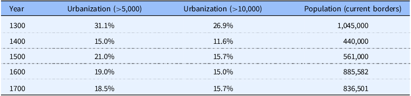

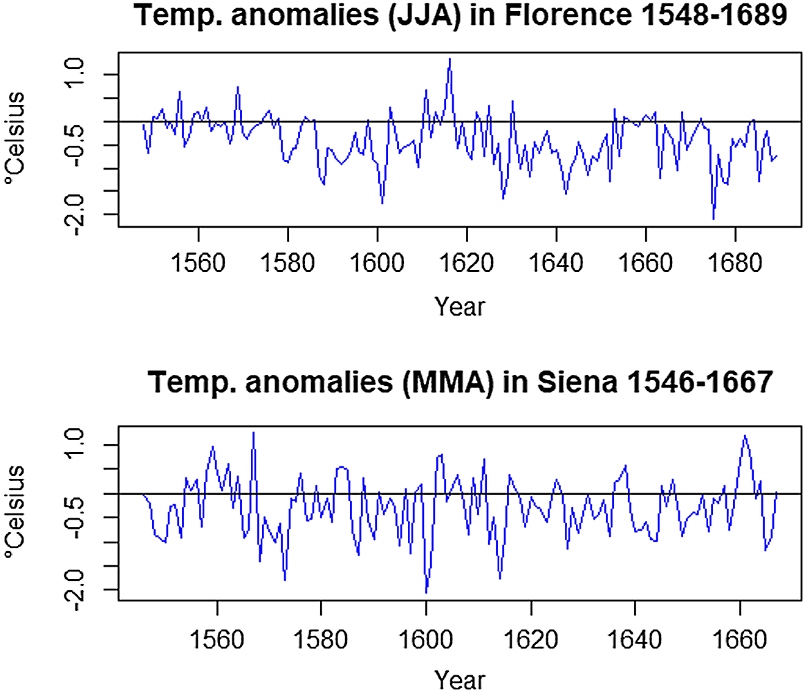


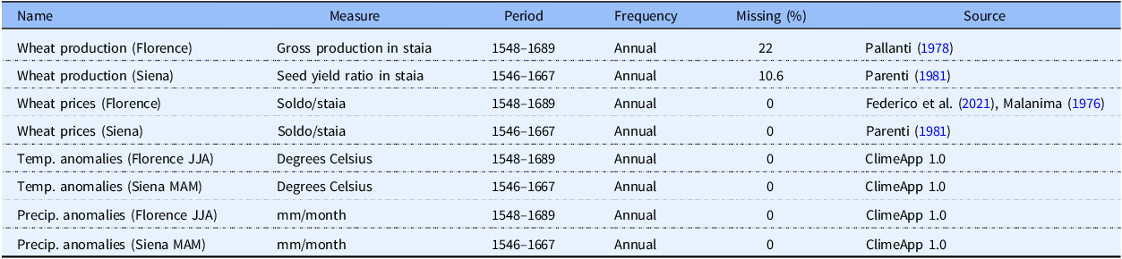

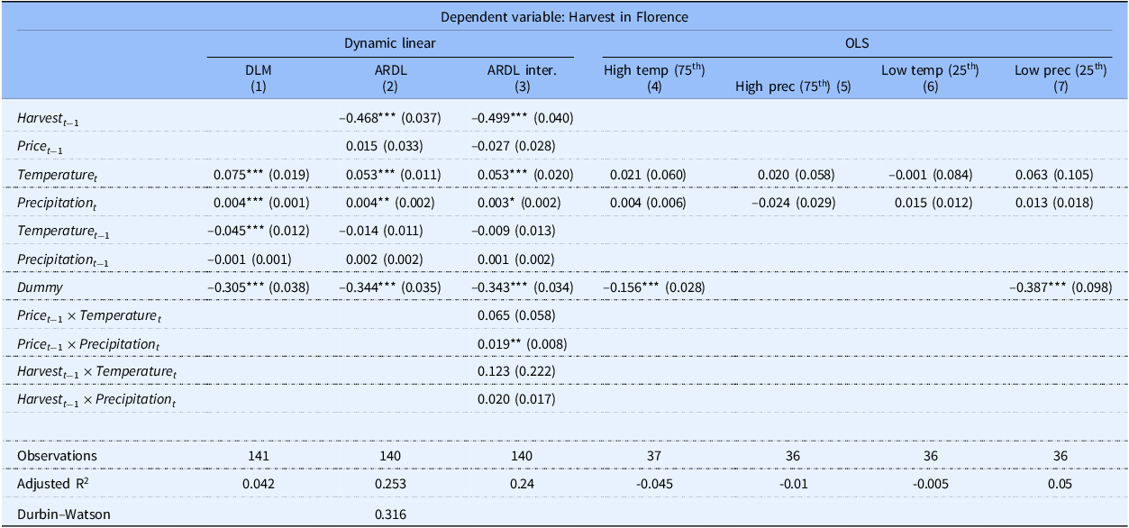
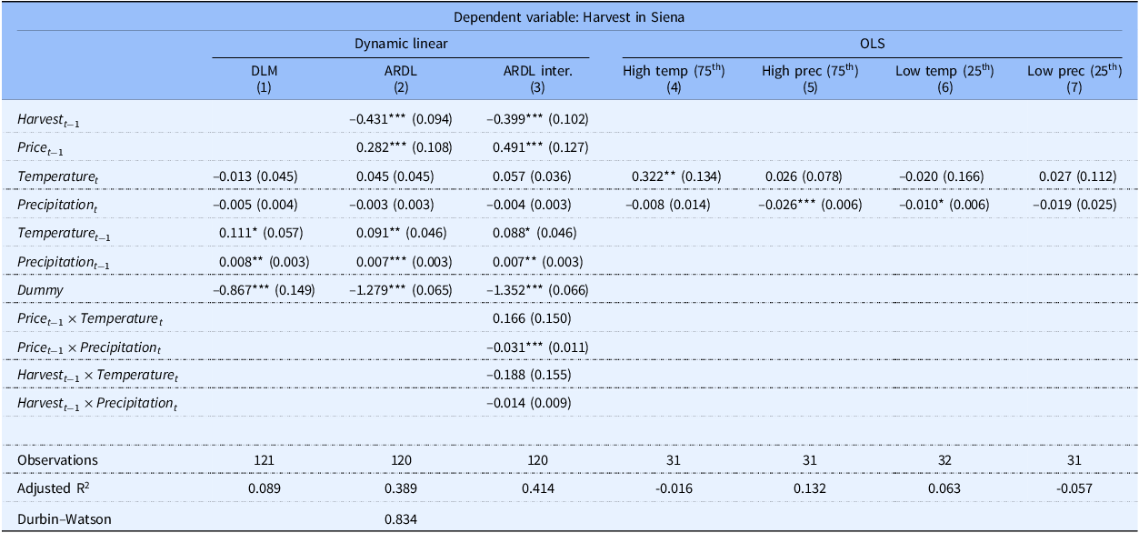

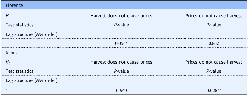

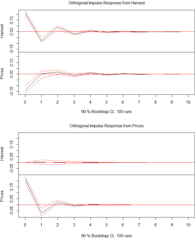

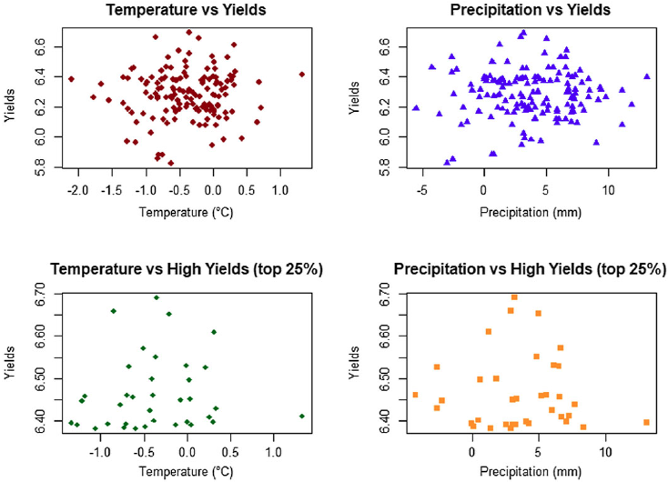
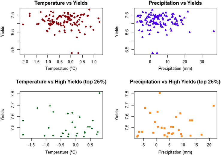

 Open access