


1. Introduction
Design teams are motivated to thoroughly explore the design space, which is believed to increase the likelihood of developing an effective design. Shah, Smith, & Vargas-Hernandez (Reference Shah, Smith and Vargas-Hernandez2003) developed outcome-based evaluation metrics that can be used to determine how well the method (a) explores the design space and (b) expands the design space. After reviewing the literature and considering the fact that domain experts can recognize “good” ideas, they propose four separate effectiveness measures: the novelty, variety, quantity and quality of the ideas generated using the method. For convenience in the rest of this paper, we will refer to Shah et al. by the first letters of each of their last names (SVS), an abbreviation that is often used in the literature.
These terms are defined by SVS:
-
• “Novelty is a measure of how unusual or unexpected an idea is as compared to other ideas.”
-
• “Variety is a measure of the explored solution space during the idea generation process.”
-
• “Quantity is the total number of ideas generated.”
-
• “Quality, in this context, is the measure of the feasibility of an idea and how close it comes to meet[ing] the design specifications.”
Two of these measures, novelty and quality, are explicitly listed as characteristics of an individual idea, although there is also a measure of set quality. The other two, variety and quantity, are measures of the set. If we are to evaluate the effectiveness of an ideation method, we must have measures of the set, rather than just measures of the individual ideas in the set, as the output of an ideation method is a set of ideas. As will be described later, set-specific measures help to indicate how well a given ideation method facilitates the design team’s exploration of the design space.
Both novelty and variety refer to a reference solution space – the actual or potential design space. As described above, novelty is evaluated by comparing the idea to the solution space; novel ideas expand the solution space. Variety is evaluated by determining how much solution space is explored.
SVS’s metrics have been widely used to identify excellent ideation practices. Idea sets with high variety, novelty, quality and quantity are regularly used as examples of, or goals for, good design outcomes (Fu, Sylcott, & Das Reference Fu, Sylcott and Das2019; Blösch-Paidosh & Shea Reference Blösch-Paidosh and Shea2021; Deo et al. Reference Deo, Blej, Kirjavainen and Hölttä-Otto2021; Miller et al. Reference Miller, Hunter, Starkey, Ramachandran, Ahmed and Fuge2021; Song et al. Reference Song, Soria Zurita, Nolte, Singh, Cagan and McComb2021; Schauer, Fillingim, & Fu Reference Schauer, Fillingim and Fu2022; Lee et al. Reference Lee, Daly, Vadakumcherry and Rodriguez2023; Ma et al. Reference Ma, Grandi, McComb and Goucher-Lambert2023; Yuan, Marion, & Moghaddam Reference Yuan, Marion and Moghaddam2023; Das et al. Reference Das, Huang, Xu and Yang2024).
As we have used SVS’s metrics in our design education and research (Anderson, Anderson, & Jensen Reference Anderson, Anderson and Jensen2019; Stapleton et al. Reference Stapleton, Owens, Mattson, Sorensen and Anderson2019; Anderson et al. Reference Anderson, Chanthavane, Broshkevitch, Braden, Bassford, Kim, Fantini, Konig, Owens and Sorensen2022; Mattson et al. Reference Mattson, Geilman, Cook-Wright, Mabey, Dahlin and Salmon2024), we have found some practical limitations to the specific metrics proposed by SVS. These limitations include the following:
-
• The lack of a method to calculate a novelty score for a set.
-
• The lack of a method for determining when two ideas are insufficiently different to be counted separately.
-
• The inability to determine how much an individual idea adds to the variety of the set.
-
• The calculated variety is divided by the number of ideas in the set, so in some sense it is the “average” variety.
-
• The novelty calculation requires a consistent functional decomposition for all the ideas under consideration, which makes SVS difficult to apply to idea sets containing highly divergent ideas.
This paper proposes axioms for metrics for each of these set attributes that reflect best practices in ideation and appropriately reward preferred ideation behavior. We then propose evaluation methods and aggregation functions that satisfy the axioms when applied to ideas placed in a design tree (defined in “Design Trees”). Broadly, these accomplish the following:
-
• Calculate the novelty of an idea.
-
• Calculate the novelty of an idea set based on the novelties of the individual ideas and the design tree relationships.
-
• Calculate the variety of an idea set.
-
• Determine how much an individual idea contributes to the set variety.
-
• Calculate the quality of an idea.
-
• Calculate the quality of an idea set based on the qualities of the individual ideas.
-
• Calculate the quantity of ideas in a set, accounting for their relationships with other ideas.
Note that for each of SVS’s four metrics, we address both the individual ideas and the set of ideas.
The evaluation of novelty, variety and quality generally involves subjective decisions. We propose specific questions that evaluators answer in order to provide as much consistency as possible to these subjective evaluations.
The aggregation functions presented in this paper are used to calculate set properties based on the individual idea properties and the tree relationships were developed to match axioms for ideal behavior of the aggregation functions. The axioms were created consistent with the principles that (a) it is always better to have more ideas, greater variety, more novelty and more quality, and (b) one should not be able to artificially influence the score of the idea set by either adding or removing ideas that are low in variety, novelty or quality.
1.1. Aims
There are four related aims of this work. The first aim is to define axioms about the evaluation of idea sets that describe the behavior of set metrics that will encourage good ideation practices. The second aim is to define evaluation methods for quality, quantity, novelty and variety that can be easily performed on early-stage ideas and have clear operational definitions that lend themselves to future AI evaluation. The third aim is to develop aggregation functions for set quantity, quality, novelty and variety that ensure the axioms are met. The final aim is to present software tools that support the evaluation methods and implement the aggregation functions.
1.2. Significance
As a result of this work, the software tools can be used to repeatably evaluate large idea sets for variety, novelty, quality and quantity. The ability to perform this evaluation helps design researchers as they seek tools to improve ideation. These evaluations can also help designers consider whether their idea set is of sufficient quality to move forward to further design stages.
2. Nomenclature
-
 $ \alpha $
-
Basic design space fraction for an idea; as
$ i $
goes to
$ \infty $
,
$ {f}_i $
goes to
$ \alpha $
-
$ \beta $
-
Parameter for reducing
$ {f}_i $
based on the number of family members.
$ \beta $
governs the rate at which
$ {f}_i $
goes to
$ \alpha $
-
$ {\epsilon}_i $
-
Bonus fraction added to
$ \alpha $
for family member
$ i $
;
$ {\epsilon}_i $
is
$ 1-\alpha $
for family member 1 and decreases to zero for family member
$ \infty $
-
$ {f}_a $
-
Average fraction of
$ {\Omega}_l $
explored by each idea in a family will be less than 1 -
$ {f}_i $
-
Fraction of
$ {\Omega}_l $
uniquely explored by idea
$ i $
; will be less than or equal to 1 -
$ {f}_t $
-
Total fraction of
$ {\Omega}_l $
explored ideas in a family will be greater than or equal to 1 -
$ l $
-
Tree level number
-
$ m $
-
Number of family members
-
$ {m}_c $
-
Number of children for an element
-
$ n $
-
Novelty for an idea, without respect to the level or the number of siblings in the design tree
-
$ N $
-
Total novelty for a tree
-
$ {N}_B $
-
Branch novelty: the total novelty of a branch whose head is the element under consideration
-
$ {N}_{B_c} $
-
Branch novelty for a branch whose head is a child of the element under consideration
-
$ {N}_D $
-
Descendant novelty: the sum of the branch novelties for all children of the element under consideration
-
$ {N}_{D_c} $
-
Descendant novelty for a child of the element under consideration
-
$ {N}_E $
-
Element novelty for an idea placed in the tree. It is a function of the idea novelty
$ n $
and the level and number of siblings in the design tree -
$ {N}_{E_c} $
-
Element novelty for a child of the element under consideration
-
$ {\Omega}_l $
-
The nominal amount of design space occupied by an idea at level
$ l $
, neglecting any overlap with closely related ideas at that level -
$ P $
-
Composite scoring points for novelty of an idea, considering its scarcity in both the current design context and another context where the idea is commonly used. Novel ideas have high values of
$ P $
-
$ q $
-
Quality of an idea
-
$ {q}_{th} $
-
Quality threshold for quality ideas. Ideas with
$ q\le {q}_{th} $
are considered low-quality ideas -
$ Q $
-
Quality of a set of elements
-
$ {Q}_B $
-
Total quality of a branch of the tree whose head is the element under consideration
-
$ {Q}_{B_c} $
-
Total quality of a branch of the tree whose head is a child of the element under consideration
-
$ {Q}_E $
-
Set quality of an element
-
$ {S}_c $
-
Scarcity of an idea in the current design context. Common ideas have low scarcity, rare ideas have high scarcity
-
$ {S}_f $
-
Scarcity of an idea in a context other than the current design context, where the idea is most commonly used. Common ideas have low scarcity, rare ideas have high scarcity
-
$ u $
-
Idea uniqueness
-
$ U $
-
Set quantity: the number of unique ideas in the set
-
$ {U}_B $
-
Set quantity of a branch: the number of unique ideas in a branch whose head is the element under consideration
-
$ {U}_{B_c} $
-
The number of unique ideas in a branch whose head is a child of the element under consideration
-
$ V $
-
Total variety for a tree
-
$ {V}_B $
-
Branch variety: the total variety created by a branch whose head is the element under consideration.
-
$ {V}_{B_c} $
-
Branch variety for a branch whose head is a child of the element under consideration
-
$ {V}_D $
-
Descendant variety: the sum of the branch varieties for the children of the element under consideration
-
$ {V}_E $
-
Element variety: The variety created by the presence of some element in a design tree.
-
$ {V}_{E_c} $
-
Element variety for a child of the element under consideration
-
$ {X}_{i,l} $
-
Amount of design space uniquely explored by family member
$ i $
on tree level
$ l $
.


3. Literature review
Shah et al. (Reference Shah, Smith and Vargas-Hernandez2003) laid the groundwork for quantitatively measuring ideation effectiveness as part of the ideation research process. They clearly identified four factors that are important to effective ideation: novelty, quality, quantity and variety. They also proposed specific methods for evaluating novelty for each idea in the set, variety in a group of ideas, quality of a group of ideas and quantity of a set. Many authors have built on SVS’s groundbreaking work to propose improvements in implemented ideation metrics, as described in this section.
3.1. Novelty
Sarkar & Chakrabarti (Reference Sarkar and Chakrabarti2011) focus on novelty. They consider the novelty of a product to be evaluated relative to existing products that meet the same need. They evaluate both functions and structures to determine the level of novelty for the product. They focus on identifying the novelty of an idea, rather than of a set of ideas. They also recognize that design creativity involves both novelty and usefulness.
Sluis-Thiescheffer et al. (Reference Sluis-Thiescheffer, Bekker, Eggen, Vermeeren and De Ridder2016) applied SVS’s novelty calculations to actual data resulting from young children’s design activities. They found some problems with novelty scores, including trivial solutions that have high novelty scores, solutions that have different novelty scores depending on their method of generation, and that there is a relatively narrow distribution of novelty scores, which means we know very little about actual novelty. Instead of a continuous novelty rating for each idea, they propose a binary score (novel, not novel).
Hernandez, Shah, & Smith (Reference Hernandez, Shah and Smith2010) introduce two possible metrics for set novelty: the average novelty of the ideas in the set (average novelty) and the novelty of the most novel idea in the set (best novelty). They make no recommendation as to which is best, and consider that each of the set-based novelty metrics contributes a different view of the set novelty.
Jagtap et al. (Reference Jagtap, Larsson, Hiort, Olander and Warell2015) introduce individual average novelty (IAN), which evaluates ideas only relative to a specific individual idea set, as compared with SVS’s average novelty (AN), which evaluates ideas relative to all available idea sets for a given design challenge. They study the interdependency between novelty and variety for both of these novelty metrics.
Ahmed et al. (Reference Ahmed, Ramachandran, Fuge, Hunter and Miller2018) use pairwise comparisons of ideas to place a small set of ideas on an idea map. They then combine the ratings of multiple raters to identify the ideas with the highest novelty.
3.2. Variety
Nelson et al. (Reference Nelson, Wilson, Rosen and Yen2009) found SVS’s variety metric to be flawed. They claim that, using the SVS variety metric and evaluation approach, it was possible for an idea set with subjectively low variety to receive an erroneously high variety score. They also found that average variety scores are flawed, and therefore propose to use total, rather than normalized variety. They attempt to resolve the problems with SVS’s measure by using different weights for the various tree levels, but provided limited justification that the selected weights were correct.
Verhaegen et al. (Reference Verhaegen, Vandevenne, Peeters and Duflou2015) noted that when idea distributions (trees) were unbalanced, SVS’s and Nelson’s methods both led to problems. They propose the use of a Shannon entropy measure at each level of the tree to calculate variety and provide an online software tool for testing new metrics.
Ahmed et al. (Reference Ahmed, Ramachandran, Fuge, Hunter and Miller2020) suggest that tree-based methods of variety evaluation are unreliable and recommend that entropy-based methods be used instead. They estimated the ground truth variety by creating subsets from a ground set of design items, having human raters make pairwise comparisons of the subsets, and calculating tree-based metrics for the subsets. They find that the Herfindahl–Hirschman Index for Design (HHID) shows better accuracy and discrimination and can be used to identify high-variety subsets.
Ahmed & Fuge (Reference Ahmed and Fuge2017) seek to obtain ranked sets of ideas for diversity and quality, with a goal of obtaining a relatively small set of ideas with high diversity and quality that can serve as a base for future ideation. They demonstrate three methods of numerically calculating similarity and show that these similarity ratings can form the basis of optimal searches for high-diversity, high-quality idea sets.
Henderson et al. (Reference Henderson, Helm, Jablokow, McKilligan, Daly and Silk2017) define a variety metric that evaluates the amount of design space covered by looking at the scores for ideas on other metrics as coordinates in an
 $ n $
-dimensional space. This provides a quantitative measure for variety, but makes variety a dependent parameter of the other metrics evaluated for the set.
$ n $
-dimensional space. This provides a quantitative measure for variety, but makes variety a dependent parameter of the other metrics evaluated for the set.
3.3. Quality
Cheeley et al. (Reference Cheeley, Weaver, Bennetts, Caldwell and Green2018) focused on quality scores and attempted to match ratings to ground truth. They identified two fundamental elements of quality: effectiveness and feasibility. They performed a statistical test to select relative weightings for effectiveness and quality that would allow quality rankings using their formula to match intuitive quality rankings by expert raters. This study showed that quality could be reliably evaluated by evaluating effectiveness and feasibility.
Kudrowitz & Wallace (Reference Kudrowitz and Wallace2013) identified three attributes of quality early-stage ideas: novel, feasible and useful. They evaluated individual product ideas, rather than the complete set of ideas. They considered this evaluation to be a first-pass evaluation.
Reinig, Briggs, & Nunamaker (Reference Reinig, Briggs and Nunamaker2007) focus on the measurement of set quality. They address the importance of identifying unique ideas, and then describe a few known methods for evaluating idea quality, and then discuss three possible set quality metrics: sum-of-quality, average-quality and good-idea-count. They demonstrate that good-idea-count is superior to the other two set quality metrics.
Toh & Miller (Reference Toh and Miller2014) assess idea quality on a five-point scale: does it achieve the desired outcome, is it technically feasible, is it easy to execute, and is it a significant improvement over the existing design. They use the average quality of the ideas for the quality of the set. They assess novelty in two classes: form-based and function-based. They use the average novelty of the ideas for the quality of the set. They evaluated the effect of physical examples and interactions on the novelty and quality of the resulting ideas.
Some researchers – including Patel et al. (Reference Patel, Summers, Morkos and Karmakar2024) – have acknowledged the challenge of predicting how well an early-stage concept will meet design requirements. Given this challenge, Patel et al. (Reference Patel, Summers, Morkos and Karmakar2024) have used addressment as a surrogate for quality, where addressment is the quantity of design requirements the concept addresses.
3.4. Quantity
All the reviewed papers that measured quantity simply counted the number of ideas listed in the set, with no adjustments for nearly identical ideas. We believe that when two ideas are close enough to one another, they should not be counted as distinct ideas. We found no references in the literature that attempted to adjust quantity measures for closely related ideas.
3.5. Weaknesses of literature metrics
Some methods for evaluating idea sets for SVS’s attributes display weaknesses in their use for evaluating idea sets. For example, using the average idea quality as a measure of the set quality means that the number of low-quality ideas will affect the set quality measure. Similarly, using the average quality of the top Y% of the ideas as the set quality measure means that a high-quality idea that is not in the top Y% will have no effect on the set quality measure. Thus, these methods reward discarding low-quality ideas from the set.
Using the count-of-quality proposed by Reinig et al. makes the quality evaluation binary – high-quality ideas get a count of 1; other ideas get a count of 0. This draws no distinction between extremely high-quality ideas and moderately high-quality ideas. This lack of distinction can be problematic.
The average novelty and individual average novelty scores described above will both drop as low-novelty ideas are added to the set. But low-novelty ideas do not decrease the exploration of the design space; they just do not increase the exploration.
When average or other normalized variety scores are used, the number of low-variety ideas is important to the overall variety score. However, the presence of low-variety ideas should not detract from the contribution to variety provided by other ideas in the set. Further, as Nelson et al. have observed, when level weightings are arbitrarily chosen, variety calculations can be inconsistent with subjective variety evaluations.
If overlap between closely related ideas is not considered, quantity can be artificially inflated by making many ideas that are virtually, but not exactly, identical.
3.6. Summary of literature
Many authors have provided methods for evaluating the SVS attributes. However, none have all of the attributes desired for our work, namely:
-
• The ability to evaluate both individual ideas and the set of ideas for all metrics
-
• An a priori description of how the aggregate scoring of an idea set should vary as the individual ideas vary
-
• The ability to quickly evaluate a large number of ideas that have a relatively low level of detail
-
• A well-defined procedure for making subjective judgments, thus helping to increase consistency between raters
-
• Set metrics that encourage the inclusion of all ideas, whether good or bad, in the set to be evaluated
Therefore, we define both simple idea evaluation tools and axiom-based aggregation functions that achieve these goals.
4. Ideas and aggregation functions
We begin by defining ideas, kinds of aggregation functions and axioms. These definitions are general; they apply to any set of ideas that can be classified by level of abstraction of ideas and similarity (or distance) between ideas.
For purposes of this paper, we define a design idea to be any idea that contributes to the definition of a solution for a design problem. A fully defined conceptual design could be a design idea. A principle that may be used to develop many conceptual designs could be a design idea. A single detail that could be added to a conceptual design could be a design idea.
Design teams can communicate their ideas in many different ways. The most common ways we have found are through words and/or sketches. We allow the team to define the boundaries of a design idea. The content of a single sketch or a single written description is considered a design idea for purposes of our analysis. For brevity, in the rest of this paper, we use the term idea as a synonym for design idea.
An idea set is the complete set of ideas produced during ideation activities intended to develop solutions to a design problem. When multiple teams are working on a particular design problem, each team will have a team idea set, and we can also consider idea sets resulting from combining two or more team idea sets.
For purposes of evaluating variety and novelty, ideas are placed into an idea space. The idea space reflects two important characteristics of design ideas: the level of abstraction of the idea and the similarity of or distance between different ideas. Any means of organizing ideas that reflect these two characteristics can be used to evaluate individual ideas for novelty, variety, quality and quantity. Further, aggregation functions can be developed to combine the individual evaluations into evaluations of set novelty, variety, quality and quantity.
4.1. Aggregation functions
Aggregation functions are used to calculate the properties of a set of ideas based on the characteristics of the individual ideas. Higher scores on the aggregation functions correspond to higher quality, quantity, novelty and variety. Aggregation functions should be designed so that the scores encourage good ideation practices.
For the best possible ideation, the free flow of ideas is encouraged. During ideation, ideas should not be filtered for quality or novelty, because even objectively bad ideas can serve as triggers for better ideas.
Consider a hypothetical situation where design ideation is a formal competition between teams. The teams will be judged on a numeric score for novelty, variety, quality and quantity. The numeric score will be calculated from the novelty, variety, quality and quantity of the individual ideas using aggregation functions. The goal is to find aggregation functions that will encourage desired ideation behaviors and ignore undesired ideation behaviors. Poor ideas should not be penalized, because teams should not be filtering ideas during ideation. The desired behavior of aggregation functions is that they will always reward adding additional ideas and never reward filtering or removing ideas.
Desirable idea evaluation and aggregation functions share the following characteristics:
-
• For any set of ideas, the aggregate score should never be increased by removing low-scoring ideas. This characteristic is necessary to discourage idea filtering either during or after ideation.
-
• Duplicate ideas should not affect the aggregate score for any metrics.
-
• Adding ideas should never reduce the aggregate score for a metric.
-
• Ideas at higher levels of abstraction explore (and if novel, expand) the design space more than ideas at lower levels of abstraction. This is because an idea at a high level of abstraction contains within it the seeds of many less abstract ideas.
-
• Ideas that are closely related contribute less to the exploration and expansion of design space than ideas that are distantly related.
-
• Novelty and quality of an idea can be evaluated independently of the location of the idea in the idea space.
-
• When considering the novelty of a set, both the novelty of an idea and the idea’s location in the idea space should be considered.
5. Axioms for ideation metrics
Based on the desirable characteristics of aggregation functions described above, axioms for set-based metrics of novelty, variety, quality and quantity are presented in this section. As axioms, they cannot be proven, but they are believed to be self-evident. In all cases, the axioms describe how the set-based metrics should change as ideas are added to the set. These axioms should apply to any set of ideas that can be classified by level of abstraction and similarity. They are not limited to tree-based set organization.
5.1. Axioms of variety
We propose the following axioms to describe how variety should change when adding new elements to an idea set:
-
Axiom V-1: Adding a unique entry at any level of abstraction should increase the total variety of the idea set. As a corollary, removing a unique entry at any level of abstraction should reduce the total variety of the set.
-
Axiom V-2: Adding a unique entry at a higher level of abstraction should increase the total variety more than adding a unique entry at a lower level.
-
Axiom V-3: Adding a unique entry at a given level of abstraction that is similar to many other ideas should increase the total variety less than adding a unique entry at the same abstraction level that is different from other ideas.
5.2. Axioms of novelty
We propose four axioms that describe how novelty should change when adding new elements to an idea set. These axioms recognize that novelty describes the expansion of design space, so both the amount of space occupied by an idea and the novelty of the idea will affect the set novelty.
-
Axiom N-1: At a given location in the idea space, an added idea with high novelty adds more to the set novelty than an added idea with low novelty.
-
Axiom N-2: A novel idea at a high level of abstraction adds more to the set novelty than an idea of equivalent novelty at a low level of abstraction.
-
Axiom N-3: An idea with a given novelty located far from other ideas in the idea space adds more to the set novelty than an idea with the same novelty located close to other ideas in the idea space.
-
Axiom N-4: The set novelty should be increased by adding a novel idea. It should be unchanged by adding an idea with zero novelty. As a corollary, the set novelty should never be increased by removing an idea.
5.3. Axioms of quantity
The following axioms are proposed for set quantity scores:
-
Axiom U-1: Duplicates of previously counted ideas should not be counted again when determining set quantity.
-
Axiom U-2: A unique idea added to the tree at a low abstraction level should add the same quantity as a unique idea added at a high abstraction level.
-
Axiom U-3: Only ideas generated by members of the team should be included in the set quantity. Ideas that may be generated by those evaluating the quantity should not add to the set quantity.
5.4. Axioms of set quality
The following axioms are proposed for set quality scores:
-
Axiom Q-1: High-quality ideas should increase the set quality more than moderate- or low-quality ideas
-
Axiom Q-2: Removing low-quality ideas from the set should not increase the set quality; adding low-quality ideas to the set should not decrease the set quality.
-
Axiom Q-3: Regardless of the number of high-quality ideas in the set, adding a high-quality idea should increase the set quality.
When these axioms are met by appropriate aggregation functions, the desired behaviors from “Aggregation Functions” will be achieved.
5.5. Axiom violations with legacy methods
To demonstrate the value of our methodology, we will now show the conditions under which the Axioms are not met with certain legacy methods, particularly SVS, because it is so well-known.
5.5.1. Variety
In Shah et al. (Reference Shah, Smith and Vargas-Hernandez2003), the SVS method is used to evaluate variety for a set with 11 ideas that result in two branches at the physical principle level, five branches at the working principle level, six branches at the embodiment level and four branches at the detail level. With SVS, these abstraction levels are scored as 10, 6, 3 and 1, respectively. Thus, the total Variety score is calculated as:
 $$ {M}_3=\left(\left(2\ast 10\right)+\left(5\ast 6\right)+\left(6\ast 3\right)+\left(4\ast 1\right)\right)/11=72/11=6.54 $$
If one of the branches is removed from the detail level, the calculation becomes:
 $$ {M}_3^{\ast }=\left(\left(2\ast 10\right)+\left(5\ast 6\right)+\left(6\ast 3\right)+\left(3\ast 1\right)\right)/10=71/10=7.1 $$
The SVS variety score has increased as a result of removing an idea, which violates Axiom V-1.
5.5.2. Novelty
SVS does not explicitly include a method for calculating a set novelty score, so there is no basis for evaluating SVS against these axioms. We believe it is useful to have a set novelty score, and necessary if researchers are going to use metrics to compare ideation methods. Later work (Nelson et al. (Reference Nelson, Wilson, Rosen and Yen2009), Hernandez et al. (Reference Hernandez, Shah and Smith2010) and Jagtap et al. (Reference Jagtap, Larsson, Hiort, Olander and Warell2015)) suggests average novelty as an idea set metric. Average novelty would fail to meet Axiom N-2 and Axiom N-3 because it would not account for location in the idea space. Further, it is trivial to show that adding a low-novelty idea would reduce the average novelty score, which would violate Axiom N-4. Hernandez et al. (Reference Hernandez, Shah and Smith2010) propose Best Novelty as a complementary metric, but it also fails to meet Axiom N-4, because any novel ideas that are less novel than the most novel idea add nothing to the score.
5.5.3. Quantity
SVS considers an idea to include a leaf element from the tree along with all of its parent elements. Only ideas that differ in at least one level are considered distinct. Thus, SVS meets all of the axioms. We wish to have the possibility of considering a single element at any level of the tree as an idea, which requires a different algorithm for determining idea quantity.
5.5.4. Quality
The SVS method calculates set quality through a weighted sum of component scores that reflect how well ideas meet certain functions or characteristics. In Shah et al. (Reference Shah, Smith and Vargas-Hernandez2003), an example is presented of four ideas (A-D) that are evaluated for manufacturability and minimum weight, which have a relative weighting of 2 and 1, respectively. The minimum weight scores for ideas A-D are 3.57, 6.14, 1.0 and 10, respectively. The manufacturability scores are 10, 8, 4 and 1, respectively. Thus, the total Quality score is calculated as:
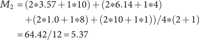 $$ {\displaystyle \begin{array}{c}{M}_2=\left(2\ast 3.57+1\ast 10\right)+\left(2\ast 6.14+1\ast 4\right)\\ {}\hskip1.5em +\left(2\ast 1.0+1\ast 8\right)+\left(2\ast 10+1\ast 1\right)\Big)/4\ast \left(2+1\right)\\ {}=64.42/12=5.37\end{array}} $$
If idea C is removed from the set, the calculation becomes:
 $$ {\displaystyle \begin{array}{c}{M}_2^{\ast }=\Big(\left(2\ast 3.57+1\ast 10\right)+\left(2\ast 6.14+1\ast 4\right)\\ {}\hskip17em +\left(2\ast 10+1\ast 1\right)\Big)/3\ast \left(2+1\right)\\ {}\hskip15.5em =54.42/9=6.05\end{array}} $$
The SVS quality score has increased as a result of removing an idea. It is similarly trivial to show that adding a 5th idea that is low quality would decrease the set quality score (a 5th idea with a weighted quality score of 10, like idea C, would result in a set quality score of 4.96). This violates Axiom Q-2. Because the SVS quality calculation is essentially a weighted average, it is also easy to show that it does not meet Axiom Q-3.
6. Design trees, exploration of design space and aggregation functions
6.1. Design trees
A common way of representing the structure in an idea set is to use a tree structure (sometimes called a “genealogy tree”) (Shah et al. Reference Shah, Smith and Vargas-Hernandez2003; Nelson et al. Reference Nelson, Wilson, Rosen and Yen2009; Verhaegen et al. Reference Verhaegen, Vandevenne, Peeters and Duflou2015; Ahmed et al. Reference Ahmed, Ramachandran, Fuge, Hunter and Miller2020).
A tree is a structure consisting of elements and edges. Elements are nodes in the design tree. There are two different types of elements in a design tree. Idea elements are ideas generated by the design team that have been placed as nodes in the tree. Organizational elements are nodes that have been placed in the tree during the analysis of an idea set to ensure that each element has a parent element. Edges connect elements at different levels of the tree, indicating a relationship between the elements. Levels in the tree range from the lowest level, which contains the most detailed information, to the highest level, which contains the most general information. When an edge connects two elements, the element at the higher level is considered a parent in the relationship, while the element at the lower level is considered a child in the relationship. A parent can have multiple children, but a child can have only one parent. A family of elements is defined as a set of elements sharing a common parent. An element with no children is considered a leaf element of the tree. A branch of the tree consists of an element and all of its descendants.
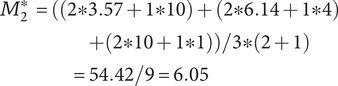
Figure 1 shows a simple genealogy tree. Elements are shown as circles. Leaf elements are labeled with the letter L. Families are enclosed in vertical dashed ovals. Branches are enclosed in polygons with rounded corners.
A sample four-level design tree. The level increases from right to left. Elements are shown by circles; their numbering is arbitrary. Leaf elements have an L following the element number. Families (groups of elements sharing a common parent, and which may have only a single member) are enclosed by dashed lines. They are labeled with F plus the level of the family. Branches are shown by shaded polygons with rounded corners. They are labeled with B plus the element number of the root element in the branch. There are eight leaf elements, seven families and seven branches in this tree.
A design tree is created by placing design ideas into a tree as elements of the tree. In this paper, when we evaluate the characteristics of an idea independent of its location in the tree, we calculate the idea properties. In contrast, when we evaluate the characteristics of an idea considering its relationships as an element of the tree, we calculate the element properties.
In order to evaluate the exploration and expansion of the design space (variety and novelty), we organize the idea set into a hierarchical tree structure. The structure we use is called an objective–principle–embodiment–detail (OPED) tree. Note that any tree structure would work in place of the OPED tree. For example, the physical principle – working principle – embodiment – detail tree used by Shah et al. (Reference Shah, Smith and Vargas-Hernandez2003) would work just as well. Every idea in the set is placed in the tree as an idea element at a particular tree level with an edge connecting it to a parent element at the next-higher level of the tree. Organizing the ideas in this fashion may require the evaluator to add organizational elements to the tree to ensure that each idea element in the tree has a parent. This is necessary to implement the scoring algorithm that follows, but does not bias the scoring, as will be demonstrated below.
For this paper, we define the levels in the OPED tree as follows:
Objective level: The desired outcome driving the ideation, which, on its own, describes the benefit provided by any idea in the set to the user or customer. This should be common to all ideas in the set. The objective describes what is to be done, not how it is to be done.
If we were doing a design project for removing ice, snow, and frost from a car windshield, an appropriate objective might be “Obtain an ice-free windshield.”
Principle level: A top-level statement of how the objective is to be achieved. A principle must be general enough that there can be multiple ways of embodying the principle. It often contains a verb as part of the principle description. One way of identifying a principle is to use the following statement and fill in the blank: “An idea could achieve the objective by __________________.”
For the objective “Obtain an ice-free windshield,” principles might include “Remove ice,” “Melt ice,” “Prevent ice formation,” and “Prevent ice adhesion.”
Embodiment level: A solution idea expressed in tangible or visible form. A way to think about an embodiment is that it has sufficient detail that it can be communicated in a concept sketch (which could apply to product, process or software design). The embodiment generally consists of a noun and one or more adjectives. The embodiment must represent a specific object.
For the example design, an embodiment might be “Ice scraper,” or “Windshield cover.”
Detail level: A solution idea that adds to, but does not fundamentally change, the embodiment. If the detail is removed, the embodiment remains.
From the example, consider a design idea for “Ice scraper with hand-warming mitten attached.” This would be a detail under the embodiment “Ice scraper.”
The decision between embodiment and detail is partly subjective, because both the embodiment and the detail are expressed in tangible or visible form. However, the tangible form of a detail adds something that is not required to be part of the embodiment.
As described above, the Objective level contains the desired outcome, not ideas for achieving the desired outcome. Thus, the Objective is not part of the generated ideas and serves only as an organizational element. The trees in this paper have only a single objective, but if desired, a tree can be created with multiple objectives.
It is anticipated that during ideation, there will often be ideas generated at the principle, embodiment and detail levels. However, if the team has not explicitly placed the ideas into a tree structure, it is unlikely that the idea elements will properly complete the design tree. For a well-formed tree, every element must ultimately be linked to the objective through a series of ancestors. Thus, every detail needs a parent embodiment, every embodiment needs a parent principle, and every principle needs a parent objective. During the analysis of the idea set, organizational elements will be added to the tree as needed to provide a parent for each idea element of the set. Guidelines for evaluating the relationships between ideas are given in “Idea Uniqueness.”
6.2. Design trees and design space exploration
Recall that SVS indicates that variety is a measure of how well the ideas explore the design space and novelty is a measure of how well the ideas expand the design space. The OPED tree is a representation of the explored region of design space. If novelty scores are assigned to individual ideas, the novelty can be used to estimate how much the design space is expanded. The detailed framework for doing this is described in “Evaluating and Aggregating Variety (Exploration of Design Space)” and “Evaluating and Aggregating Novelty (Expansion of Design Space).”
We recognize that the OPED tree cannot describe the total design space. It can only describe the explored space (because the ideas that have been generated represent exploration). Given this limitation, the OPED trees can only produce relative measures, but we believe that even the relative measures are useful.
The fundamental basis of this method is the recognition that every idea, regardless of its tree level, explores a finite amount of design space. Closely related ideas will overlap one another in the design space, so the amount of space explored per idea is less than for distantly related ideas. The total amount of explored space can be calculated from the sum of the individual spaces minus the overlapping spaces. The amount of explored design space is used in the calculation of set variety and set novelty.
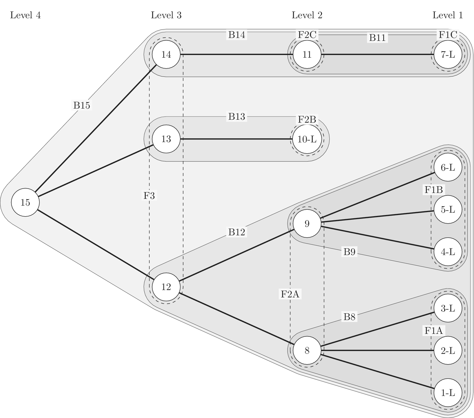
Figure 2 shows a schematic representation of the design space captured by a design tree. Circles in the figure represent the amount of design space explored by an idea. In this figure, ideas at the principle level (
 $ l=3 $
) are labeled
$ l=3 $
) are labeled
 $ {P}_i $
, ideas at the embodiment level (
$ {P}_i $
, ideas at the embodiment level (
 $ l=2 $
) are labeled
$ l=2 $
) are labeled
 $ {E}_{ij} $
(where index
$ {E}_{ij} $
(where index
 $ i $
is the index of the principle that is the parent of the embodiment) and ideas at the detail level (
$ i $
is the index of the principle that is the parent of the embodiment) and ideas at the detail level (
 $ l=3 $
) are labeled
$ l=3 $
) are labeled
 $ {D}_{ijk} $
(where index
$ {D}_{ijk} $
(where index
 $ ij $
is the index of the embodiment, i.e., the parent of the detail). To help make the parent/child relationships clearer, a line connects each parent to the cluster of ideas that are its children.
$ ij $
is the index of the embodiment, i.e., the parent of the detail). To help make the parent/child relationships clearer, a line connects each parent to the cluster of ideas that are its children.
Schematic representation of the design space explored by ideas in a tree structure. Two important concepts are illustrated: (1) individual ideas at higher levels of the tree explore more space than individual ideas at lower levels of the tree, and (2) closely related ideas overlap one another in the design space. The circles for principles, embodiments and details represent the amount of design space explored by an element at the principle (
 $ l=3 $
), embodiment (
$ l=3 $
), embodiment (
 $ l=2 $
) and detail (
$ l=2 $
) and detail (
 $ l=1 $
) levels, respectively. This figure does not indicate the absolute location of any of the ideas in the design space.
$ l=1 $
) levels, respectively. This figure does not indicate the absolute location of any of the ideas in the design space.
Although drawn as a two-dimensional space, the design tree space has no axes. The absolute location of an idea is arbitrary. However, the relative locations of two ideas are not arbitrary. Closely related ideas (siblings in the design tree) overlap one another. Distantly related ideas (those that are not siblings) do not overlap. The only conclusion we can draw about the distance between non-overlapping ideas is that their separation is greater than the characteristic size of the explored space for an idea at a given level.
The area of the rectangle in the figure represents the amount of design space available for meeting the objective. Each idea explores a part of the area of the design space shown by a circle in the figure. The size of the circle represents
 $ {\Omega}_l $
, which is the amount of design space explored by an idea at level
$ {\Omega}_l $
, which is the amount of design space explored by an idea at level
 $ l $
. Principles (
$ l $
. Principles (
 $ l=3 $
) explore more design space (and thus have larger circles representing
$ l=3 $
) explore more design space (and thus have larger circles representing
 $ {\Omega}_3 $
) than embodiments (
$ {\Omega}_3 $
) than embodiments (
 $ l=2 $
, circle of
$ l=2 $
, circle of
 $ {\Omega}_2 $
), which explore more design space than details (
$ {\Omega}_2 $
), which explore more design space than details (
 $ l=1 $
, circle of
$ l=1 $
, circle of
 $ {\Omega}_1 $
). When ideas are closely related, their circles overlap. When they are distantly related, their circles will not overlap. When circles overlap, the amount of design space uniquely explored by a given idea is reduced by the overlap with closely related ideas.
$ {\Omega}_1 $
). When ideas are closely related, their circles overlap. When they are distantly related, their circles will not overlap. When circles overlap, the amount of design space uniquely explored by a given idea is reduced by the overlap with closely related ideas.
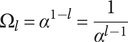
6.3. Design space for family members
When a first child is added to an element in the tree, a family consisting of that child is created. Each member of a family can be considered to explore an amount of design space (including overlaps) of
 $ {\Omega}_l $
, which depends on the level of the family. However, due to overlaps with family members, the amount of design space uniquely explored by an idea (called
$ {\Omega}_l $
, which depends on the level of the family. However, due to overlaps with family members, the amount of design space uniquely explored by an idea (called
 $ {X}_{i,l} $
) may be less than
$ {X}_{i,l} $
) may be less than
 $ {\Omega}_l $
. We define the member fraction
$ {\Omega}_l $
. We define the member fraction
 $ {f}_i $
to be
$ {f}_i $
to be
 $ {X}_{i,l}/{\Omega}_l $
. As shown schematically in Figure 3, the member fraction for the first member of the family (
$ {X}_{i,l}/{\Omega}_l $
. As shown schematically in Figure 3, the member fraction for the first member of the family (
 $ {f}_1 $
) is 1. The member fraction for family member
$ {f}_1 $
) is 1. The member fraction for family member
 $ 2 $
will be less than 1 and is denoted
$ 2 $
will be less than 1 and is denoted
 $ {f}_2 $
.
$ {f}_2 $
.
 $ {f}_3 $
, the member fraction for family member
$ {f}_3 $
, the member fraction for family member
 $ 3 $
, is less than
$ 3 $
, is less than
 $ {f}_2 $
. Exact formulas for
$ {f}_2 $
. Exact formulas for
 $ {f}_i $
are provided later. Note that the total design space uniquely allocated to family member
$ {f}_i $
are provided later. Note that the total design space uniquely allocated to family member
 $ i $
at level
$ i $
at level
 $ l $
is given by
$ l $
is given by
 $ {X}_{i,l}={f}_i{\Omega}_l $
.
$ {X}_{i,l}={f}_i{\Omega}_l $
.
Schematic representation of member fraction, total fraction and average fraction for a set of three ideas in a family at level
 $ l $
. For this representation, the area of the circle is
$ l $
. For this representation, the area of the circle is
 $ {\Omega}_l $
, and the fraction is a part of the circle. In part (a), we see the three overlapping ideas on the same level. All three circles have the same explored area of
$ {\Omega}_l $
, and the fraction is a part of the circle. In part (a), we see the three overlapping ideas on the same level. All three circles have the same explored area of
 $ {\Omega}_l $
. Member 1 has a member fraction
$ {\Omega}_l $
. Member 1 has a member fraction
 $ {f}_1 $
of 1, as all the space is assumed to be uniquely explored by Member 1. Member 2 has a member fraction
$ {f}_1 $
of 1, as all the space is assumed to be uniquely explored by Member 1. Member 2 has a member fraction
 $ {f}_2 $
less than 1 due to its overlap with member 1, so its uniquely explored design space is less. Member 3 has a member fraction
$ {f}_2 $
less than 1 due to its overlap with member 1, so its uniquely explored design space is less. Member 3 has a member fraction
 $ {f}_3 $
less than
$ {f}_3 $
less than
 $ {f}_2 $
due to overlap with both members 1 and 2. Part (b) shows the total design space explored by the family, which is a multiple of
$ {f}_2 $
due to overlap with both members 1 and 2. Part (b) shows the total design space explored by the family, which is a multiple of
 $ {\Omega}_l $
called
$ {\Omega}_l $
called
 $ {f}_t $
. Part (c) shows the average fraction
$ {f}_t $
. Part (c) shows the average fraction
 $ {f}_a $
for each member when we have no basis for determining which idea explores the most design space.
$ {f}_a $
for each member when we have no basis for determining which idea explores the most design space.

As shown in Figure 3(b), the total design space explored by a family will be greater than the space explored by any single idea in the family. The total family space is a multiple of
 $ {\Omega}_l $
called the total fraction
$ {\Omega}_l $
called the total fraction
 $ {f}_t $
.
$ {f}_t $
.
 $ {f}_t $
is the sum of the member fractions for all family members.
$ {f}_t $
is the sum of the member fractions for all family members.
 $$ {f}_t=\sum \limits_{i=1}^m{f}_i $$
where
 $ m $
is the number of family members.
$ m $
is the number of family members.
As we add members to the family, the total fraction
 $ {f}_t $
increases, but the member fraction for each additional member
$ {f}_t $
increases, but the member fraction for each additional member
 $ {f}_i $
decreases, due to greater overlap of ideas in the family. This is shown schematically in Figure 3.
$ {f}_i $
decreases, due to greater overlap of ideas in the family. This is shown schematically in Figure 3.
When evaluating the novelty of design ideas, we number the ideas according to decreasing novelty. The most novel idea then explores the most design space, and as the novelty of ideas decreases, the amount of design space explored by the less-novel idea decreases as well.
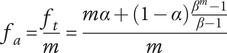
When evaluating variety, the numbering scheme for members is arbitrary (i.e., there is no reason for calling one idea member 1 and another idea member 2). This makes it inappropriate to assume that one idea explores more design space than another. In this case, we calculate an average fraction
 $ {f}_a $
to assign to every member of the family, as shown in Figure 3(c).
$ {f}_a $
to assign to every member of the family, as shown in Figure 3(c).
 $ {f}_a $
is the total fraction divided by the number of members.
$ {f}_a $
is the total fraction divided by the number of members.
 $$ {f}_a=\frac{f_t}{m}=\frac{\sum_{i=1}^m{f}_i}{m} $$
7. Applying the axioms to design trees
As previously described, design trees contain levels and families. Tree levels are measures of the level of abstraction for an idea. A higher level in the tree corresponds to a higher level of abstraction. The number of family members in the design tree is used as the number of closely related ideas. In the design tree analysis, we have no independent measure of the distance between families, so our distances are relative, rather than absolute.
When applying these tree elements to the axioms, we obtain the axioms for use with design trees.
7.1. Tree variety
-
Axiom TV-1: Adding a unique entry at any level of the tree should increase the total variety of the idea set.
-
Axiom TV-2: Adding a unique entry at a higher level of the tree should increase the total variety more than adding a unique entry at a lower level.
-
Axiom TV-3: Adding a unique entry at a given level of the tree that has many family members should increase the total variety less than adding a unique entry at the same level with few family members.
An example may help explain the meaning of the last axiom. Figure 4 shows partial results of an ideation session focused on improving home security. As shown, an embodiment idea of a bio-inspired mobile robot sentry was generated (
 $ {E}_{11} $
). Detailed ideas for this embodiment included robot dog (
$ {E}_{11} $
). Detailed ideas for this embodiment included robot dog (
 $ {D}_{111} $
), robot chicken (
$ {D}_{111} $
), robot chicken (
 $ {D}_{112} $
), robot lion (
$ {D}_{112} $
), robot lion (
 $ {D}_{113} $
), robot snake (
$ {D}_{113} $
), robot snake (
 $ {D}_{114} $
) and robot cat (
$ {D}_{114} $
) and robot cat (
 $ {D}_{115} $
), for a total of five details.
$ {D}_{115} $
), for a total of five details.
A sample design tree showing a subset of the ideas generated. The objective is to improve home security. The only principle shown in the figure is detecting intrusion. There are two embodiments shown:
 $ {E}_{11} $
and
$ {E}_{11} $
and
 $ {E}_{12} $
.
$ {E}_{12} $
.
 $ {E}_{11} $
has four details, with a potential fifth shown in gray.
$ {E}_{11} $
has four details, with a potential fifth shown in gray.
 $ {E}_{12} $
has one detail, with a potential second shown in gray. As discussed in the text, adding
$ {E}_{12} $
has one detail, with a potential second shown in gray. As discussed in the text, adding
 $ {D}_{122} $
should add more variety to the set than adding
$ {D}_{122} $
should add more variety to the set than adding
 $ {D}_{116} $
. Also, if
$ {D}_{116} $
. Also, if
 $ {D}_{122} $
and
$ {D}_{122} $
and
 $ {D}_{116} $
are equally novel ideas, adding
$ {D}_{116} $
are equally novel ideas, adding
 $ {D}_{122} $
should add more novelty to the set than adding
$ {D}_{122} $
should add more novelty to the set than adding
 $ {D}_{116} $
.
$ {D}_{116} $
.

An alternative embodiment idea is a system of stationary sensors scattered throughout the house (
 $ {E}_{12} $
). The only detailed idea for this embodiment is a camera network (
$ {E}_{12} $
). The only detailed idea for this embodiment is a camera network (
 $ {D}_{121} $
).
$ {D}_{121} $
).
An alternative idea at the detail level for a robot kangaroo (
 $ {D}_{116} $
) should add less variety to the set than an idea at the detail level for a stationary LiDAR detection system (
$ {D}_{116} $
) should add less variety to the set than an idea at the detail level for a stationary LiDAR detection system (
 $ {D}_{122} $
).
$ {D}_{122} $
).
7.2. Tree novelty
-
Axiom TN-1: At a given location in the design tree, an idea with high novelty adds more to the set novelty than an idea with low novelty.
-
Axiom TN-2: A novel idea at a high level of the tree adds more to the set novelty than an equivalent idea at a low level of the tree.
-
Axiom TN-3: An idea with a given novelty in a small family adds more to the set novelty than an idea with the same novelty in a large family.
-
Axiom TN-4: The set novelty should be increased by adding a novel idea. It should be unchanged by adding an idea with zero novelty. As a corollary, the set novelty should never be increased by removing an idea.
7.3. Tree quantity
-
Axiom TU-1: Duplicates of previously counted ideas should not be counted again when determining set quantity.
-
Axiom TU-2: The set quantity should not depend on the tree level at which the ideas are expressed.
-
Axiom TU-3: Organizational elements added to the tree by evaluators should not affect the set quantity.
7.4. Tree quality
-
Axiom TQ-1: High-quality ideas should increase the set quality more than moderate-quality ideas.
-
Axiom TQ-2: Removing low-quality ideas from the set should not increase the set quality; adding low-quality ideas to the set should not decrease the set quality.
-
Axiom TQ-3: Regardless of the number of high-quality ideas in the set, adding a high-quality idea should increase the set quality.
Note that the tree quality axioms are identical to the general quality axioms, as the quality axioms refer to neither the level of abstraction nor the distance from adjacent ideas. However, we list them here for convenience.
8. Evaluating and aggregating variety (exploration of design space)
In this section, we discuss how variety is evaluated and aggregated in the context of a design tree. If some other organization of the idea space is used, new evaluation and aggregation functions will need to be defined and used.
SVS explain that variety is a measure of the explored design space. Each idea that is developed adds to the exploration of design space. The assessment of the explored design space cannot be completed without considering the relationships of the different ideas. Thus, we cannot calculate an idea variety (variety that ignores the location in the tree). Instead, we first calculate the element variety (variety of the idea in its location in the tree). We then calculate the branch varieties for successively higher branches of the tree (elements with all their descendants), culminating in the total variety for the set. In addition, because each idea increases the explored design space, the variety of an idea set increases as the number of principles, embodiments and details in the idea set increases.
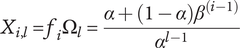
8.1. Element variety
As described in “Design Space for Family Members,” each idea placed in the tree to form an element explores a certain region of design space, the amount of which depends on the level of the element and the number of siblings. We call the amount of design space explored by an element the explored space
 $ {X}_{i,l} $
.
$ {X}_{i,l} $
.
 $$ {X}_{i,l}={f}_i{\Omega}_l $$
where
 $ {\Omega}_l $
is the amount of design space explored by each idea at level
$ {\Omega}_l $
is the amount of design space explored by each idea at level
 $ l $
, and
$ l $
, and
 $ {f}_i $
is the fraction of
$ {f}_i $
is the fraction of
 $ {\Omega}_l $
uniquely explored by member element
$ {\Omega}_l $
uniquely explored by member element
 $ i $
in the family.
$ i $
in the family.
In this section, we develop functions for
 $ {\Omega}_l $
and
$ {\Omega}_l $
and
 $ {f}_i $
that can be used with simple aggregation functions to meet the variety axioms. We will start with
$ {f}_i $
that can be used with simple aggregation functions to meet the variety axioms. We will start with
 $ {f}_i $
.
$ {f}_i $
.
The function
 $ {f}_i $
should have a value of 1 for the first family member, and decrease with increasing value of
$ {f}_i $
should have a value of 1 for the first family member, and decrease with increasing value of
 $ i $
. However, it should have a non-zero asymptote, because regardless of the number of family members, an additional unique idea will increase the amount of design space explored.
$ i $
. However, it should have a non-zero asymptote, because regardless of the number of family members, an additional unique idea will increase the amount of design space explored.
The function chosen to meet these criteria
 $ {f}_i $
is:
$ {f}_i $
is:
 $$ {f}_i=\alpha +\left(1-\alpha \right){\beta}^{\left(i-1\right)} $$
where
 $ \alpha $
and
$ \alpha $
and
 $ \beta $
are parameters with values between 0 and 1 that are used to adjust the amount of design space allocated to members of a family.
$ \beta $
are parameters with values between 0 and 1 that are used to adjust the amount of design space allocated to members of a family.
Note that for
 $ i=1 $
,
$ i=1 $
,
 $ {f}_i=1 $
; for
$ {f}_i=1 $
; for
 $ i=\infty $
,
$ i=\infty $
,
 $ {f}_i $
has the limiting value
$ {f}_i $
has the limiting value
 $ \alpha $
. Thus
$ \alpha $
. Thus
 $ \alpha $
describes the lower limit of the design space a single idea can occupy.
$ \alpha $
describes the lower limit of the design space a single idea can occupy.
 $ \beta $
is a shape parameter that defines how rapidly
$ \beta $
is a shape parameter that defines how rapidly
 $ {f}_i $
falls toward its limiting value of
$ {f}_i $
falls toward its limiting value of
 $ \alpha $
. The choice of specific values for
$ \alpha $
. The choice of specific values for
 $ \alpha $
and
$ \alpha $
and
 $ \beta $
is discussed in “Choosing Values for Evaluation Parameters.”
$ \beta $
is discussed in “Choosing Values for Evaluation Parameters.”
The total fraction for the family is given by the sum of the member fractions in the family:
 $$ {f}_t=\sum \limits_{i=1}^m{f}_i=\sum \limits_{i=1}^m\left[\alpha +\left(1-\alpha \right){\beta}^{\left(i-1\right)}\right]= m\alpha +\left(1-\alpha \right)\sum \limits_{k=0}^{m-1}{\beta}^k= m\alpha +\left(1-\alpha \right)\frac{\beta^m-1}{\beta -1} $$
where
 $ m $
is the number of family members (the identity for this finite series is found in Abramowitz & Stegun (Reference Abramowitz and Stegun1972)).
$ m $
is the number of family members (the identity for this finite series is found in Abramowitz & Stegun (Reference Abramowitz and Stegun1972)).
In order to meet Axiom TV-2,
 $ {\Omega}_l $
is chosen to ensure that the minimum possible explored design space for an idea at level
$ {\Omega}_l $
is chosen to ensure that the minimum possible explored design space for an idea at level
 $ l+1 $
is greater than the maximum possible explored space for an element at level
$ l+1 $
is greater than the maximum possible explored space for an element at level
 $ l $
. The minimum explored design space at level
$ l $
. The minimum explored design space at level
 $ l+1 $
is for an idea with infinite family members, where the member fraction is
$ l+1 $
is for an idea with infinite family members, where the member fraction is
 $ \alpha $
. Thus the minimum value of explored design space on level
$ \alpha $
. Thus the minimum value of explored design space on level
 $ l+1 $
is
$ l+1 $
is
 $ {X}_{\infty, l+1}=\alpha {\Omega}_{l+1} $
. The maximum explored design space at level
$ {X}_{\infty, l+1}=\alpha {\Omega}_{l+1} $
. The maximum explored design space at level
 $ l $
is for the first idea in a family
$ l $
is for the first idea in a family
 $ {X}_{1,l}={\Omega}_l $
. Setting
$ {X}_{1,l}={\Omega}_l $
. Setting
 $ {X}_{\infty, l+1}={X}_{1,l} $
we obtain a recurrence relation for
$ {X}_{\infty, l+1}={X}_{1,l} $
we obtain a recurrence relation for
 $ \Omega $
:
$ \Omega $
:
 $$ {\Omega}_{l+1}={\Omega}_l/\alpha $$
Without loss of generality, we can define
 $ {\Omega}_1=1 $
, then
$ {\Omega}_1=1 $
, then
 $$ {\Omega}_l={\alpha}^{1-l}=\frac{1}{\alpha^{l-1}} $$
With this substitution, equation (7) becomes
 $$ {X}_{i,l}={f}_i{\Omega}_l=\frac{\alpha +\left(1-\alpha \right){\beta}^{\left(i-1\right)}}{\alpha^{l-1}} $$
When calculating variety, there is no basis for deciding which idea is the first, and which is the last, so we do not use a different value
 $ {f}_i $
for each family member. Instead, we use the average fraction for the family
$ {f}_i $
for each family member. Instead, we use the average fraction for the family
 $ {f}_a $
, given by
$ {f}_a $
, given by
 $$ {f}_a=\frac{f_t}{m}=\frac{m\alpha +\left(1-\alpha \right)\frac{\beta^m-1}{\beta -1}}{m} $$
We then define the variety for each idea in the family to be an average amount of explored design space per family member
 $ {X}_{a,l} $
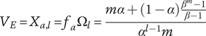 $$ {V}_E={X}_{a,l}={f}_a{\Omega}_l=\frac{m\alpha +\left(1-\alpha \right)\frac{\beta^m-1}{\beta -1}}{\alpha^{l-1}m} $$
As described in “Choosing Values for Evaluation Parameters,” for this paper
 $ \beta =0.32 $
and
$ \beta =0.32 $
and
 $ \alpha =0.46 $
. Table 1 lists the member fraction, total fraction and average fraction for members 1–10 given these values of
$ \alpha =0.46 $
. Table 1 lists the member fraction, total fraction and average fraction for members 1–10 given these values of
 $ \beta $
and
$ \beta $
and
 $ \alpha $
.
$ \alpha $
.
Member fraction, total fraction and average fraction for family sizes up to 10 with
 $ \alpha =0.46 $
and
$ \alpha =0.46 $
and
 $ \beta =0.32 $

8.2. Branch variety
Starting at the leaf elements and working up to higher levels of the tree, the element variety can be aggregated into branch variety. For any element, we can calculate a branch variety, which is the sum of the element variety and the branch varieties for all children of the element.
The branch variety of an element is given by
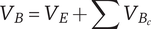 $$ {V}_B={V}_E+\sum {V}_{B_c} $$
where
 $ {V}_B $
is the branch variety of an element, and
$ {V}_B $
is the branch variety of an element, and
 $ {V}_{B_c} $
is the branch variety of a child of the element.
$ {V}_{B_c} $
is the branch variety of a child of the element.
For convenience, we can show the descendant variety
 $ {V}_D $
for an element, which is the sum of the branch varieties for all children of the element.
$ {V}_D $
for an element, which is the sum of the branch varieties for all children of the element.
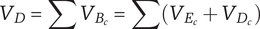 $$ {V}_D=\sum {V}_{B_c}=\sum \left({V}_{E_c}+{V}_{D_c}\right) $$
where
 $ {V}_{E_c} $
and
$ {V}_{E_c} $
and
 $ {V}_{D_c} $
are the element variety and descendant variety, respectively, for a child of the element.
$ {V}_{D_c} $
are the element variety and descendant variety, respectively, for a child of the element.
8.3. Total variety
The total variety for a tree (
 $ V $
) is equal to the sum of the branch varieties for all elements at the highest level of the tree.
$ V $
) is equal to the sum of the branch varieties for all elements at the highest level of the tree.
8.4. Meeting the variety axioms
We can demonstrate that all three axioms are met by the given aggregation function.
Axiom TV-1: Adding a unique entry to any level of the tree should increase the total variety of the tree.
This axiom is met because each idea (regardless of its level) has a positive element variety, and the total variety is the sum of the element varieties for all elements. Thus, adding an element will increase the total variety.
Axiom TV-2: Adding a unique entry to a higher level of the tree should increase the total variety more than adding a unique entry to a lower level.
This axiom is met because the maximum element variety added by an idea at level
 $ l $
is
$ l $
is
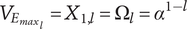 $$ {V}_{E_{{\mathit{\max}}_l}}={X}_{1,l}={\Omega}_l={\alpha}^{1-l} $$
The minimum variety added by a new element
 $ i $
at level
$ i $
at level
 $ l+1 $
is given by
$ l+1 $
is given by
 $$ \underset{i\to \infty }{\lim}\left[\alpha +\left(1-\alpha \right){\beta}^{\left(i-1\right)}\right]{f}_i=\alpha {\Omega}_{l+1}={\alpha \alpha}^{1-\left(l+1\right)}={\alpha}^{1-l} $$
For a finite design tree (and all design trees are finite)
 $ i<\infty $
, so
$ i<\infty $
, so
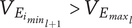 $ {V}_{E_{i_{{\mathit{\min}}_{l+1}}}}>{V}_{E_{{\mathit{\max}}_l}} $
.
$ {V}_{E_{i_{{\mathit{\min}}_{l+1}}}}>{V}_{E_{{\mathit{\max}}_l}} $
.
Axiom TV-3 Adding a unique entry at a given level to a family with many members should increase the total variety less than adding a unique entry at the same level to a family with few members.
To show that this axiom is met, consider the effect of adding an idea
 $ A $
at level
$ A $
at level
 $ l $
in a family with
$ l $
in a family with
 $ {m}_1 $
existing members. The added variety will be
$ {m}_1 $
existing members. The added variety will be
 $ {V}_E $
for this new idea, which is
$ {V}_E $
for this new idea, which is
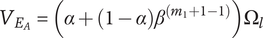 $ {V}_{E_A}=\left(\alpha +\left(1-\alpha \right){\beta}^{\left({m}_1+1-1\right)}\right){\Omega}_l $
. Now consider adding a different idea
$ {V}_{E_A}=\left(\alpha +\left(1-\alpha \right){\beta}^{\left({m}_1+1-1\right)}\right){\Omega}_l $
. Now consider adding a different idea
 $ B $
also at level
$ B $
also at level
 $ l $
in a family with
$ l $
in a family with
 $ {m}_2 $
members, where
$ {m}_2 $
members, where
 $ {m}_2<{m}_1 $
. The added variety will be
$ {m}_2<{m}_1 $
. The added variety will be
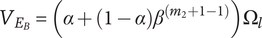 $ {V}_{E_B}=\left(\alpha +\left(1-\alpha \right){\beta}^{\left({m}_2+1-1\right)}\right){\Omega}_l $
. If
$ {V}_{E_B}=\left(\alpha +\left(1-\alpha \right){\beta}^{\left({m}_2+1-1\right)}\right){\Omega}_l $
. If
 $ \Delta V={V}_{E_B}-{V}_{E_A} $
is positive, the axiom is met.
$ \Delta V={V}_{E_B}-{V}_{E_A} $
is positive, the axiom is met.
 $$ \Delta V=\left(\alpha +\left(1-\alpha \right){\beta}^{\left({m}_2\right)}\right){\Omega}_l-\left(\alpha +\left(1-\alpha \right){\beta}^{\left({m}_1\right)}\right){\Omega}_l=\left(1-\alpha \right)\left({\beta}^{\left({m}_2\right)}-{\beta}^{\left({m}_1\right)}\right){\Omega}_l $$
As all three terms in the product above are positive,
 $ \Delta V $
is positive. Thus, Axiom V-3 is met.
$ \Delta V $
is positive. Thus, Axiom V-3 is met.
Note that the variety axioms are all met regardless of the specific values chosen for
 $ \alpha $
and
$ \alpha $
and
 $ \beta $
. However, the actual numerical value for the variety of a set of ideas will vary with
$ \beta $
. However, the actual numerical value for the variety of a set of ideas will vary with
 $ \alpha $
and
$ \alpha $
and
 $ \beta $
. The same is true for other parameters in our evaluation for novelty and quality. The rationale for the specific values chosen for these evaluation parameters is discussed in “Choosing Values for Evaluation Parameters.”
$ \beta $
. The same is true for other parameters in our evaluation for novelty and quality. The rationale for the specific values chosen for these evaluation parameters is discussed in “Choosing Values for Evaluation Parameters.”
9. Evaluating and aggregating novelty (expansion of design space)
In order to evaluate novelty, we need to see how well the design space is expanded by the ideas. There are two important aspects of novelty. The first, called the idea novelty (
 $ n $
), is the novelty of an idea, irrespective of where the idea sits in the design tree. The second aspect is the explored design space for each idea, which takes into account the location of the idea in the tree. The element novelty for an idea placed in the context of the tree is the product of the idea novelty and the explored design space for the idea. The total novelty of a set is the sum of the element novelties for each of the elements in the set.
$ n $
), is the novelty of an idea, irrespective of where the idea sits in the design tree. The second aspect is the explored design space for each idea, which takes into account the location of the idea in the tree. The element novelty for an idea placed in the context of the tree is the product of the idea novelty and the explored design space for the idea. The total novelty of a set is the sum of the element novelties for each of the elements in the set.
SVS provide two methods for measuring novelty of individual ideas. The first method evaluates a particular idea for commonality with other known ideas in the same problem space. Ideas that are infrequently seen in the reference set of ideas have a higher novelty score. This method is an effective method when comparing the results of different individuals, teams or ideation methods, and when a broad set of reference ideas for a given problem space is available. If there is no set of reference ideas, this method cannot be used. The novelty scores will depend on the reference set of ideas. If the reference set changes, the score will change. Furthermore, if the reference set is narrow compared with the universe of possible ideas, the novelty scores will be artificially inflated.
A second method proposed by SVS breaks an overall concept up into functions and then uses an expert to assign a novelty score for each of the functions. This method uses the experience of the expert in lieu of an explicit set of reference ideas as a method for assessing the novelty of the generated ideas. However, there are no guidelines for how an expert will decide the novelty of each idea. In their example, a score of 3 is given for an idea considered to be of low novelty, a score of 7 for an idea considered to be novel, and a score of 10 for an idea that was not anticipated by the rater.
In this paper, we develop an alternative method for assigning an idea novelty score. This method can be used for principles, embodiments or details, and can be applied to early design ideas, where many of the details are as yet unknown.
To calculate the novelty of a concept, Shah et al. (Reference Shah, Smith and Vargas-Hernandez2003) determine the idea realized by the concept at each level of the design tree, then calculate a weighted sum of the novelties at each level. The weightings are decided by the evaluator, and the sum of all weightings is 1.
In our work, we evaluate the novelty of each idea, regardless of the level, and then calculate an element novelty for each of the ideas by weighting the idea novelty according to the level (with the highest levels having a higher weight) and according to its relative novelty in the family, with more novel ideas having a higher weight. Following SVS, we could calculate a concept novelty by summing the element novelties for each of the elements in the concept. However, we are more interested in the novelties of the individual ideas (which are captured in the element novelties of the ideas) than in the novelties of complete concepts.
Note that SVS does not address the calculation of the novelty of a tree. In this paper, we describe a process for combining the individual idea novelties to achieve a set novelty. We believe such a measure is useful for at least two reasons: to help a team decide when the ideation has been sufficiently rich, and to make comparative evaluations of the performance of different ideation methods.
9.1. Types of novelty
As mentioned previously, there are two different types of novelty with which we are concerned, idea novelty and element novelty. The novelty of branches and complete sets of ideas can be calculated from the element novelty of the elements in the tree.
Idea novelty (
 $ n $
) is the novelty of an idea that is independent of the tree in which the idea is placed.
$ n $
) is the novelty of an idea that is independent of the tree in which the idea is placed.
Element novelty (
 $ {N}_E $
) is the novelty of an idea in the context of the design tree. The element novelty depends on both the novelty of the idea and the structure of the tree.
$ {N}_E $
) is the novelty of an idea in the context of the design tree. The element novelty depends on both the novelty of the idea and the structure of the tree.
Branch novelty (
 $ {N}_B $
) is the total element novelty of a branch of the tree headed by a particular element.
$ {N}_B $
) is the total element novelty of a branch of the tree headed by a particular element.
Novelty of a set (
 $ N $
) is the total element novelty of the set.
$ N $
) is the total element novelty of the set.
To calculate the novelty of a set of ideas, we must calculate idea novelty, element novelty and branch novelty. We address each of these novelty calculations in turn.
9.2. Idea novelty
Organizational elements (parent items that are added by the evaluators for the purpose of organizing the tree) are given a novelty value of 0. This ensures that the elements added by evaluators do not contribute to the total set novelty.
For each idea element (ideas generated by the design team) in the tree, the novelty of the idea is evaluated by methods such as those used by SVS, or by the method we propose below. Any consistent method for calculating idea novelty for an element will work with the calculations described here.
Although not required, we find it helpful to scale idea novelty to be in the interval [0,1]. One can think of the novelty score as the fraction of design space occupied by the idea that lies outside of the known design space. If the novelty is 0, the idea occupies no space outside the known space. If the novelty is 1, the idea lies entirely outside the known design space.
9.3. Evaluating idea novelty
In this section, we present a new method for evaluating idea novelty. This method is neither the SVS a priori method nor the SVS a posteriori method. Like the SVS a priori method, this method uses the rater’s experience to assign a novelty rating. However, in contrast to the SVS a priori method, the rater makes no judgments as to what ideas would be novel before making the rating. Similar to the SVS a posteriori method, each of the ideas in the set is evaluated by the rater. However, in contrast to the SVS a posteriori method, the rater’s judgment is used for each of the ideas, rather than just the frequency of occurrence of the ideas. This method allows the rater to focus on the ideas present in the idea set and follows a straightforward, albeit subjective, method.
The rater completes four steps to evaluate each idea. The four steps are:
-
1 Considering the idea exclusive of other ideas in the current set, how commonly do you believe the idea is used or proposed in this design context? Give a response of C, R or N (common, rare or never).
-
2 Describe the mechanism or technique by which the idea operates to achieve the design objective.
-
3 Can you identify another context (other than this design context) where this idea (or a very similar idea) uses the mechanism described to achieve an objective? If so, list this other context. If not, the response for this step is “None,” and the response for the next step is “N.”
-
4 How commonly do you believe this idea is used or proposed as described in this other context? Provide a response of C, R or N (common, rare or never).
In steps 1 and 4, where we evaluate the prevalence of an idea, we use the phrase used or proposed because many common ideas have never been actually implemented. For example, time machines and faster-than-light travel are well-known in science fiction, even though they have never been used in a real product. So, the idea of a time machine should not be considered rarely or never used.
The “other context” in steps 3 and 4 refers to any usage context for the idea with which the rater is familiar. There is no unique right answer to the other context question. However, the other context is specifically identified in order to help justify the prevalence evaluation.
It is possible that the evaluator cannot identify another context in which the idea is used. In this case, the response for question 3 becomes “None” and the answer to question 4 automatically becomes “N” (never).
After the rater has provided ratings of C, R or N for the idea in the design context and a similar idea in some other familiar context, the software assigns point values for both contexts,
 $ {P}_d $
for the design context and
$ {P}_d $
for the design context and
 $ {P}_o $
for the other context. The point values for a rating of C, R or N will be
$ {P}_o $
for the other context. The point values for a rating of C, R or N will be
 $ {S}_c $
,
$ {S}_c $
,
 $ {S}_r $
or
$ {S}_r $
or
 $ {S}_n $
, respectively. It is required that
$ {S}_n $
, respectively. It is required that
 $ {S}_c<{S}_r<{S}_n $
, so that rarer ideas will have a higher point score. Specific values of
$ {S}_c<{S}_r<{S}_n $
, so that rarer ideas will have a higher point score. Specific values of
 $ {S}_c $
,
$ {S}_c $
,
 $ {S}_r $
and
$ {S}_r $
and
 $ {S}_n $
are chosen as described in “Choosing Values for Evaluation Parameters.”
$ {S}_n $
are chosen as described in “Choosing Values for Evaluation Parameters.”
The novelty point value for the idea is calculated as
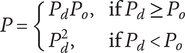 $$ P=\left\{\begin{array}{ll}{P}_d{P}_o,& \mathrm{if}\;{P}_d\ge {P}_o\\ {}{P}_d^2,& \mathrm{if}\;{P}_d<{P}_o\end{array}\right. $$
If the current design context has a lower score than the other context, the composite score is the square of the score for the design context, because rarity in another context does not increase the novelty in the design context.
The composite score
 $ P $
is then normalized to the interval [0,1] by calculating the ratio
$ P $
is then normalized to the interval [0,1] by calculating the ratio
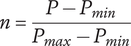 $$ n=\frac{P-{P}_{min}}{P_{max}-{P}_{min}} $$
where
 $ P $
is the composite score, and
$ P $
is the composite score, and
 $ {P}_{max}={S}_n^2 $
and
$ {P}_{max}={S}_n^2 $
and
 $ {P}_{min}={S}_c^2 $
are the maximum and minimum possible composite scores.
$ {P}_{min}={S}_c^2 $
are the maximum and minimum possible composite scores.
This composite scoring method was chosen because it allows consideration of both the specific use of an idea (the current design context) and the general use of an idea (the other context). An idea that is common in both the current context and general use has very little novelty. An idea that is rare in the current context but common in general use has some novelty. An idea that is never seen in the current context and is rare in general use has significant novelty.
9.4. Element novelty
The element novelty is the product of the design space explored by the idea and the novelty of the idea (which represents the fraction of the explored space that is novel). The amount of design space explored by an idea has been previously defined as
 $ {X}_{i,l} $
. In contrast with the variety calculation, when calculating set novelty, there is a rational basis for choosing the order of family members. We consider the first member of the family to be the one with the highest novelty. Thus, we determine the member index
$ {X}_{i,l} $
. In contrast with the variety calculation, when calculating set novelty, there is a rational basis for choosing the order of family members. We consider the first member of the family to be the one with the highest novelty. Thus, we determine the member index
 $ i $
by sorting the members in decreasing order of idea novelty. We then calculate the design space allocated to the idea, not by the average fraction, but instead by the individual fraction. Thus, the design space allocated to family member
$ i $
by sorting the members in decreasing order of idea novelty. We then calculate the design space allocated to the idea, not by the average fraction, but instead by the individual fraction. Thus, the design space allocated to family member
 $ i $
is given by
$ i $
is given by
 $$ {X}_{i,l}={f}_i{\Omega}_l $$
If there are multiple family members with equal idea novelty,
 $ {f}_i $
is the average fraction for all ideas having the same idea novelty (but not including any ideas with different novelty).
$ {f}_i $
is the average fraction for all ideas having the same idea novelty (but not including any ideas with different novelty).
The element novelty is given by
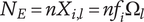 $$ {N}_E={nX}_{i,l}={nf}_i{\Omega}_l $$
9.5. Branch and set novelty
Branch novelty is the sum of the element novelty of an element and the element novelty of its descendants (
 $ {N}_D $
).
$ {N}_D $
).
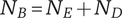 $$ {N}_B={N}_E+{N}_D $$
The element novelty of the descendants of an element is the sum of the branch novelties of the element’s children
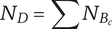 $$ {N}_D=\sum {N}_{B_c} $$
Therefore, branch novelty is given by
 $$ {N}_B={N}_E+\sum {N}_{B_c}={N}_E+\sum \left({N}_{E_c}+{N}_{D_c}\right) $$
The total novelty for a set (
 $ N $
) is the sum of the branch novelties for all elements at the highest level of the tree.
$ N $
) is the sum of the branch novelties for all elements at the highest level of the tree.
9.6. Meeting the novelty axioms
We can demonstrate that all four novelty axioms are met by the given aggregation function.
Axiom N-1: At a given location in the design tree, an idea with high novelty adds more to the set novelty than an idea with low novelty.
Consider two possible alternative ideas at a given location in design space. The first idea has idea novelty
 $ {n}_A $
; the second has idea novelty
$ {n}_A $
; the second has idea novelty
 $ {n}_B $
. Assume idea A is more novel than idea B, so
$ {n}_B $
. Assume idea A is more novel than idea B, so
 $ {n}_A>{n}_B $
. Thus, we can define
$ {n}_A>{n}_B $
. Thus, we can define
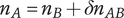 $ {n}_A={n}_B+\delta {n}_{AB} $
where
$ {n}_A={n}_B+\delta {n}_{AB} $
where
 $ \delta {n}_{AB} $
is positive.
$ \delta {n}_{AB} $
is positive.
Both ideas are in the same location in design space (member of the same family at level
 $ l $
). Define the member number for idea
$ l $
). Define the member number for idea
 $ A $
as
$ A $
as
 $ {i}_A $
and the member number for idea
$ {i}_A $
and the member number for idea
 $ B $
as
$ B $
as
 $ {i}_B $
. Because
$ {i}_B $
. Because
 $ {n}_A>{n}_B $
,
$ {n}_A>{n}_B $
,
 $ {i}_A\le {i}_B $
and
$ {i}_A\le {i}_B $
and
 $ {f}_{i_A}\ge {f}_{i_B} $
. Thus, we can define
$ {f}_{i_A}\ge {f}_{i_B} $
. Thus, we can define
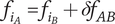 $ {f}_{i_A}={f}_{i_B}+\delta {f}_{AB} $
, where
$ {f}_{i_A}={f}_{i_B}+\delta {f}_{AB} $
, where
 $ \delta {f}_{AB} $
is non-negative.
$ \delta {f}_{AB} $
is non-negative.
Let
 $ \Delta N $
be the difference in element novelty between the alternative ideas A and B. If the difference is positive, idea A adds more novelty than idea B.
$ \Delta N $
be the difference in element novelty between the alternative ideas A and B. If the difference is positive, idea A adds more novelty than idea B.
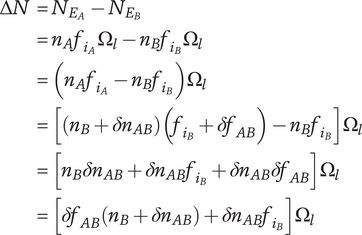 $$ {\displaystyle \begin{array}{c}\Delta N={N}_{E_A}-{N}_{E_B}\\ {}={n}_A{f}_{i_A}{\Omega}_l-{n}_B{f}_{i_B}{\Omega}_l\\ {}=\left({n}_A{f}_{i_A}-{n}_B{f}_{i_B}\right){\Omega}_l\\ {}=\left[\left({n}_B+\delta {n}_{AB}\right)\left({f}_{i_B}+\delta {f}_{AB}\right)-{n}_B{f}_{i_B}\right]{\Omega}_l\\ {}=\left[{n}_B\delta {n}_{AB}+\delta {n}_{AB}{f}_{i_B}+\delta {n}_{AB}\delta {f}_{AB}\right]{\Omega}_l\\ {}=\left[\delta {f}_{AB}\left({n}_B+\delta {n}_{AB}\right)+\delta {n}_{AB}{f}_{i_B}\right]{\Omega}_l\end{array}} $$
The first term in the square brackets is positive (if
 $ \delta {f}_{AB}>0 $
) or zero (if
$ \delta {f}_{AB}>0 $
) or zero (if
 $ \delta {f}_{AB}=0 $
). The second term in the square brackets is positive, as both of its factors are positive. Thus, the sum in the brackets is positive,
$ \delta {f}_{AB}=0 $
). The second term in the square brackets is positive, as both of its factors are positive. Thus, the sum in the brackets is positive,
 $ \Delta N $
is positive and Axiom N-1 is met.
$ \Delta N $
is positive and Axiom N-1 is met.
Axiom TN-2: A novel idea at a high level of the tree adds more to the set novelty than an idea with equivalent novelty at a low level of the tree.
Consider two alternative ideas having equal idea novelty
 $ n $
and member fraction
$ n $
and member fraction
 $ {f}_i $
, but at different levels in the tree. Idea A is at level
$ {f}_i $
, but at different levels in the tree. Idea A is at level
 $ {l}_A $
, and idea B is at level
$ {l}_A $
, and idea B is at level
 $ {l}_B $
, where
$ {l}_B $
, where
 $ {l}_A>{l}_B $
.
$ {l}_A>{l}_B $
.
We calculate the ratio of the element novelties
 $ {N}_{E_A}/{N}_{E_B} $
. If the ratio is greater than 1, idea A adds more set novelty than idea B.
$ {N}_{E_A}/{N}_{E_B} $
. If the ratio is greater than 1, idea A adds more set novelty than idea B.
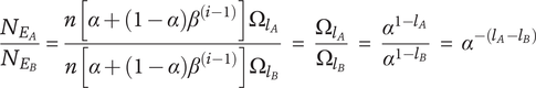 $$ \frac{N_{E_A}}{N_{E_B}}=\frac{n\left[\alpha +\left(1-\alpha \right){\beta}^{\left(i-1\right)}\right]{\Omega}_{l_A}}{n\left[\alpha +\left(1-\alpha \right){\beta}^{\left(i-1\right)}\right]{\Omega}_{l_B}}=\frac{\Omega_{l_A}}{\Omega_{l_B}}=\frac{\alpha^{1-{l}_A}}{\alpha^{1-{l}_B}}={\alpha}^{-\left({l}_A-{l}_B\right)} $$
where
 $ {l}_A-{l}_B $
is positive. By definition,
$ {l}_A-{l}_B $
is positive. By definition,
 $ \alpha <1 $
, so
$ \alpha <1 $
, so
 $ {\alpha}^{-\left({l}_A-{l}_B\right)}>1 $
, and Axiom Axiom N-2 is met.
$ {\alpha}^{-\left({l}_A-{l}_B\right)}>1 $
, and Axiom Axiom N-2 is met.
Axiom N-3: An idea with a given novelty located far from other ideas in the design tree adds more to the set novelty than an idea with the same novelty located close to other ideas in the design tree.
In the tree-based design space, closely related ideas are placed in the same family. As the number of ideas in a family increases, the overlap between ideas increases, so the ideas are more closely related.
Remember that, for novelty calculations, we consider that the more-novel ideas are added first, and the less-novel ideas are added later. Consider two alternative ideas having equal idea novelty
 $ n $
, and equal level
$ n $
, and equal level
 $ l $
. Idea A is placed in a small family
$ l $
. Idea A is placed in a small family
 $ (A) $
with a previous total of
$ (A) $
with a previous total of
 $ {m}_A $
members, and idea B is placed in a large family
$ {m}_A $
members, and idea B is placed in a large family
 $ (B) $
with a previous total of
$ (B) $
with a previous total of
 $ {m}_B $
members, where
$ {m}_B $
members, where
 $ {m}_A<{m}_B $
.
$ {m}_A<{m}_B $
.
When idea A is placed into family
 $ A $
, it becomes member
$ A $
, it becomes member
 $ {m}_A+1 $
(because it is the least-novel idea in the family at this point). When idea B is placed into family
$ {m}_A+1 $
(because it is the least-novel idea in the family at this point). When idea B is placed into family
 $ B $
it becomes member
$ B $
it becomes member
 $ {m}_B+1 $
.
$ {m}_B+1 $
.
The element novelty of idea A is given by
 $$ {N}_{E_A}={nf}_{m_A+1}{\Omega}_l $$
and the element novelty of idea B is given by
 $$ {N}_{E_B}={nf}_{m_B+1}{\Omega}_l $$
We calculate the ratio of the element novelties
 $ {N}_{E_A}/{N}_{E_B} $
. If the ratio is greater than 1, idea A adds more set novelty than idea B.
$ {N}_{E_A}/{N}_{E_B} $
. If the ratio is greater than 1, idea A adds more set novelty than idea B.
 $$ \frac{N_{E_A}}{N_{E_B}}=\frac{f_{m_A+1}}{f_{mB+1}} $$
Because
 $ {m}_A+1<{m}_B+1 $
,
$ {m}_A+1<{m}_B+1 $
,
 $ {f}_{m_A+1}>{f}_{mB+1} $
, so the ratio is greater than 1, and Axiom TN-3 is met.
$ {f}_{m_A+1}>{f}_{mB+1} $
, so the ratio is greater than 1, and Axiom TN-3 is met.
Axiom TN-4 The set novelty should never be reduced by adding an idea. As a corollary, the set novelty should never be increased by removing an idea.
When an idea is added to the set, the element novelty of the idea is added to the set. The element novelty
 $ {N}_E $
is given by
$ {N}_E $
is given by
 $$ {N}_E={nf}_i{\Omega}_l $$
As all terms in Eq. (32) are non-negative (it is possible for
 $ n $
to be 0),
$ n $
to be 0),
 $ {N}_E $
is greater than or equal to 0, and thus the novelty cannot be reduced by adding any idea. As a corollary, every idea in a set has a non-negative element novelty, so eliminating an idea cannot increase the set novelty.
$ {N}_E $
is greater than or equal to 0, and thus the novelty cannot be reduced by adding any idea. As a corollary, every idea in a set has a non-negative element novelty, so eliminating an idea cannot increase the set novelty.
10. Evaluating and aggregating quantity
Quantity is evaluated by counting the number of unique ideas in the set. Clearly, if there are two identical ideas in a set, they should not both be counted in the set quantity. In this section, we explore what makes an idea unique and thus a contributor to the set quantity. As part of evaluating quantity, an evaluator needs to eliminate redundant ideas, as described in “Mechanics of Evaluation.”
10.1. Idea uniqueness
We define the uniqueness of an idea
 $ u $
.
$ u $
.
 $ u $
has two possible values. If an idea has at least one feature that is different from all other ideas in the set,
$ u $
has two possible values. If an idea has at least one feature that is different from all other ideas in the set,
 $ u=1 $
. If all features of the idea are shared in common with at least one other idea in the set,
$ u=1 $
. If all features of the idea are shared in common with at least one other idea in the set,
 $ u=0 $
.
$ u=0 $
.
There are four general ways that two ideas can share common features, as illustrated by the Venn diagrams of features in Figure 5. In case (a), the two ideas share no common features, so they are both unique. In case (b), all of the features are found in both ideas, which means the ideas are duplicates. Duplicates should be combined into a single idea that is placed into the OPED tree.
Four different relationships two ideas can have relative to sharing common features.

In case (c), all of the features in idea 1 are found in idea 2, but idea 2 has some features not found in idea 1. In this case, idea 2 is unique but idea 1 is not, as it is contained in idea 2. This case is generally found in a parent–child tree relationship. The child idea 2 contains all the features of the parent, plus some additional features.
In case (d), ideas 1 and 2 share some common features, but each has features not found in the other. Both ideas are unique. This case is generally found in a sibling relationship. The parent contains all the common features, but each child has some unique features.
With this understanding of sharing common features, we can define the value of
 $ u $
$ u $
 $$ u=\left\{\begin{array}{cc}0,& \hskip-0.16em \mathrm{if}\hskip0.5em {m}_c>0\\ {}1,& \hskip0.22em \mathrm{if}\hskip0.5em {m}_c=0\end{array}\right. $$
where
 $ {m}_c $
is the number of children. Note that any organizational element added to the tree will have children, so
$ {m}_c $
is the number of children. Note that any organizational element added to the tree will have children, so
 $ u $
will be zero for organizational elements and organizational elements will not add to the set quantity.
$ u $
will be zero for organizational elements and organizational elements will not add to the set quantity.
10.2. Evaluating set quantity
The set quantity is the count of the unique ideas in the tree, or the sum of the idea uniqueness.
 $$ U=\sum {u}_k $$
where the sum is over all elements in the tree.
The branch quantity is the count of unique ideas in a branch, or the sum of the idea uniqueness and the branch quantity of the children:
 $$ {U}_B=u+\sum {U}_{B_C} $$
Note that we have no children if
 $ u $
is non-zero, so only one of the terms will apply for any branch.
$ u $
is non-zero, so only one of the terms will apply for any branch.
10.3. Meeting quantity axioms
Axiom TU-1: Duplicates of previously counted ideas should not be counted again when determining set quantity.
Duplicate ideas are combined into a single idea, which has a single uniqueness score (0 if it has children, 1 if it has no children).
Axiom TU-2: The set quantity should not depend on the level of detail at which the ideas are expressed.
It does not matter the level at which a unique idea is expressed; all unique ideas have a quantity score of 1, regardless of the level.
Axiom TU-3: Organizational elements added to the tree by evaluators should not affect the set quantity.
Because all parent ideas share elements with their children, they have a uniqueness score
 $ u $
of 0. Elements added to organize the tree are always parent elements and will thus not add to the set quantity.
$ u $
of 0. Elements added to organize the tree are always parent elements and will thus not add to the set quantity.
11. Evaluating and aggregating quality
As mentioned earlier, SVS describe quality as “the measure of the feasibility of an idea and how close it comes to meet[ing] the design specifications.” We believe this is a very useful definition of idea quality. However, note that this definition applies only to ideas, not idea sets. Therefore, we have developed axioms for set quality, a method for evaluating idea quality and a method for calculating element and set quality that is consistent with these axioms.
Some published methods for calculating set quality are inconsistent with these axioms. For example, using the average idea quality as a measure of the set quality means that the number of low-quality ideas will affect the set quality measure. Similarly, using the average quality of the top X% of the ideas as the set quality measure means that a high-quality idea that is not in the top X% will have no effect on the set quality measure.
Some researchers have found that a rater’s ability to evaluate an idea can be influenced by how well the idea is represented – such as the level of detail of the idea description (Hannah, Joshi, & Summers (Reference Hannah, Joshi and Summers2012)). As seen in the next section, this paper describes a simple 3-point quality evaluation scale that can be completed for ideas described at various levels of detail. The present paper does not attempt to characterize the degree to which the level of idea representation affects a rater’s ability to assess it using scales more detailed than the simple 3-point feasibility and effectiveness evaluations described in the next sections.
11.1. Idea quality
Cheeley et al. (Reference Cheeley, Weaver, Bennetts, Caldwell and Green2018) proposed a quality metric including feasibility and effectiveness. They note that having only two dimensions to rate increases the efficiency; that having separate evaluations for two important aspects of quality supports repeatability; and that these dimensions define quality in a manner consistent with the literature. For this reason, we adopted these dimensions for our quality rating.
We propose a simple, three-level evaluation for feasibility and effectiveness that combines to give a quality evaluation. It is valuable to recognize that this evaluation method is not for the purpose of choosing or improving specific design solutions. Rather, it provides details for assessing the overall quality of the ideation, as manifest in the resulting idea set.
Some researchers have found that a rater’s ability to evaluate an idea can be influenced by how well the idea is represented – such as the level of detail of the idea description (Hannah et al. (Reference Hannah, Joshi and Summers2012)). As seen in the next section, this paper describes a simple 3-point quality evaluation scale that can be completed for ideas described at various levels of detail. The present paper does not attempt to characterize the degree to which the level of idea representation affects a rater’s ability to assess it using scales more detailed than the simple 3-point feasibility and effectiveness evaluations described in the next sections.
To provide a numerical rating of idea quality, we assign feasibility (
 $ F $
) and effectiveness (
$ F $
) and effectiveness (
 $ E $
) scores based on answers to questions about feasibility and meeting design specifications:
$ E $
) scores based on answers to questions about feasibility and meeting design specifications:
-
• Considering both technical and resource limitations, how feasible is it to implement this idea to solve the design problem?
-
a. Certainly feasible:
$ F={F}_c>{F}_p $
-
b. Possibly feasible:
$ F={F}_p>0 $
-
c. Not feasible:
$ F={F}_n=0 $
-
-
• If it were implemented, what impact would the idea have in meeting the design requirements?
-
d. Major positive impact:
$ E={E}_{maj}>{E}_{min} $
-
e. Minor positive impact:
$ E={E}_{min}>0 $
-
f. No impact or negative impact:
$ E={E}_n=0 $
-


Because the composite score is the product of the feasibility and effectiveness scores, and infeasible or ineffective ideas have zero quality,
 $ {F}_n={E}_n=0 $
Feasibility and effectiveness are evaluated only for idea elements. For organizational elements,
$ {F}_n={E}_n=0 $
Feasibility and effectiveness are evaluated only for idea elements. For organizational elements,
 $ E $
and
$ E $
and
 $ F $
remain at the default value of 0. Thus, organizational elements have
$ F $
remain at the default value of 0. Thus, organizational elements have
 $ q=0 $
and do not add to the set quality.
$ q=0 $
and do not add to the set quality.
The feasibility and effectiveness scores are multiplied to give a composite idea quality score. Composite scores lie in the range
 $ \left[0,{F}_c{E}_{maj}\right] $
. Infeasible ideas and ineffective ideas have a composite score of 0. Thus, if an idea is either infeasible or has no impact on meeting requirements, it is only necessary to answer one question.
$ \left[0,{F}_c{E}_{maj}\right] $
. Infeasible ideas and ineffective ideas have a composite score of 0. Thus, if an idea is either infeasible or has no impact on meeting requirements, it is only necessary to answer one question.
The idea quality score
 $ q $
is calculated by normalizing the composite score to the range of [0,1] by dividing by the maximum possible composite score of
$ q $
is calculated by normalizing the composite score to the range of [0,1] by dividing by the maximum possible composite score of
 $ {F}_c{E}_{maj} $
.
$ {F}_c{E}_{maj} $
.
 $$ q=\frac{FE}{F_c{E}_{maj}} $$
For this paper,
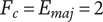 $ {F}_c={E}_{maj}=2 $
, and
$ {F}_c={E}_{maj}=2 $
, and
 $ {F}_p={E}_{min}=1 $
. The rationale behind these choices is explained in “Choosing Values for Evaluation Parameters.”
$ {F}_p={E}_{min}=1 $
. The rationale behind these choices is explained in “Choosing Values for Evaluation Parameters.”
11.2. Element quality
To calculate the set quality, we first define the element quality, which is the quality of an idea in the context of the design tree. Element quality will be zero for all low-quality elements, and it will be positive for all elements that are not considered to be low quality.
Low-quality elements are elements with an idea less than or equal to a defined quality threshold
 $ {q}_{th} $
. Ideas with quality scores above
$ {q}_{th} $
. Ideas with quality scores above
 $ {q}_{th} $
are considered to have positive quality, meaning they will add to the set quality. For this paper, we choose
$ {q}_{th} $
are considered to have positive quality, meaning they will add to the set quality. For this paper, we choose
 $ {q}_{th}=0.2 $
. The justification for this choice is given in “Choosing Values for Evaluation Parameters.”
$ {q}_{th}=0.2 $
. The justification for this choice is given in “Choosing Values for Evaluation Parameters.”
The element quality
 $ {Q}_E $
is given by
$ {Q}_E $
is given by
 $$ {Q}_E=\left\{\begin{array}{ll}0,& \mathrm{if}\;q\le {q}_{th}\\ {}\frac{q-{q}_{th}}{1-{q}_{th}},& \mathrm{if}\;q>{q}_{th}\end{array}\right. $$
Note that, like
 $ q $
,
$ q $
,
 $ {Q}_E $
lies in the interval [0,1]. The idea quality and element quality questions and results are shown in Figure 6.
$ {Q}_E $
lies in the interval [0,1]. The idea quality and element quality questions and results are shown in Figure 6.
A graphical representation of the quality calculations. Feasibility ratings and scores are shown along the top; Effectiveness ratings and scores are shown on the left. Idea quality
 $ q $
and element set quality
$ q $
and element set quality
 $ {Q}_E $
are shown in the intersection of the Feasibility column and the effectiveness row. High-quality idea scores are shaded. For this paper,
$ {Q}_E $
are shown in the intersection of the Feasibility column and the effectiveness row. High-quality idea scores are shaded. For this paper,
 $ {q}_{th}=0.2 $
.
$ {q}_{th}=0.2 $
.
Note that this definition allows for low-quality ideas (those with
 $ q\le {q}_{th} $
) that do not add to the set quality. It also allows for a range of element quality scores for those that exceed the threshold. Thus, an idea that greatly exceeds the threshold adds more quality to the set than an idea that only slightly exceeds the threshold.
$ q\le {q}_{th} $
) that do not add to the set quality. It also allows for a range of element quality scores for those that exceed the threshold. Thus, an idea that greatly exceeds the threshold adds more quality to the set than an idea that only slightly exceeds the threshold.
Also, note that the element quality
 $ {Q}_E $
can be calculated regardless of the method used to assign an idea quality
$ {Q}_E $
can be calculated regardless of the method used to assign an idea quality
 $ q $
. All that is needed to calculate
$ q $
. All that is needed to calculate
 $ {Q}_E $
is a method for calculating
$ {Q}_E $
is a method for calculating
 $ q $
and a threshold value for quality ideas
$ q $
and a threshold value for quality ideas
 $ {q}_{th} $
.
$ {q}_{th} $
.
11.3. Branch and set quality
Because the element quality will apply to all elements in the branch, the branch quality is equal to the product of the element quality and the branch quantity plus the branch qualities of its children:
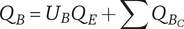 $$ {Q}_B={U}_B{Q}_E+\sum {Q}_{B_C} $$
The set quality score is the sum of the branch qualities for all elements at the highest level of the tree.
11.4. Meeting the quality axioms
We can demonstrate that all three quality axioms are met by the given aggregation function.
Axiom TQ-1: High-quality ideas should affect set quality more than moderate-quality ideas.
Items with a high quality have a higher
 $ {Q}_E $
than moderate quality ideas. Therefore, they contribute more to the set quality.
$ {Q}_E $
than moderate quality ideas. Therefore, they contribute more to the set quality.
Axiom TQ-2: Removing low-quality ideas from the set should not increase the set quality; adding low-quality ideas to the set should not decrease the set quality.
No ideas have a negative element quality score. Therefore, it is not possible to raise the set quality score by removing an idea. The lowest possible element quality score is zero, so adding low-quality ideas will not reduce the set quality.
Axiom TQ-3: Regardless of the number of high-quality ideas in the set, adding a high-quality idea should increase the set quality.
Every idea with
 $ q>{q}_{th} $
has a positive element quality
$ q>{q}_{th} $
has a positive element quality
 $ {Q}_E $
, which will increase the set quality
$ {Q}_E $
, which will increase the set quality
 $ Q $
.
$ Q $
.
12. Choosing values for evaluation parameters
As was mentioned previously, the axioms will be met for any values of the parameters that meet the requirements. However, we have chosen recommended values of the parameters for use in this study. In this section, we discuss the rationale behind the choice of these values. Table 2 provides a summary of these choices.
Numerical parameters used in this paper for calculating variety, novelty and quality scores. The axioms hold for all values of parameters that meet the requirements shown. The specific values chosen for this paper, along with a brief explanation for the choice, are shown
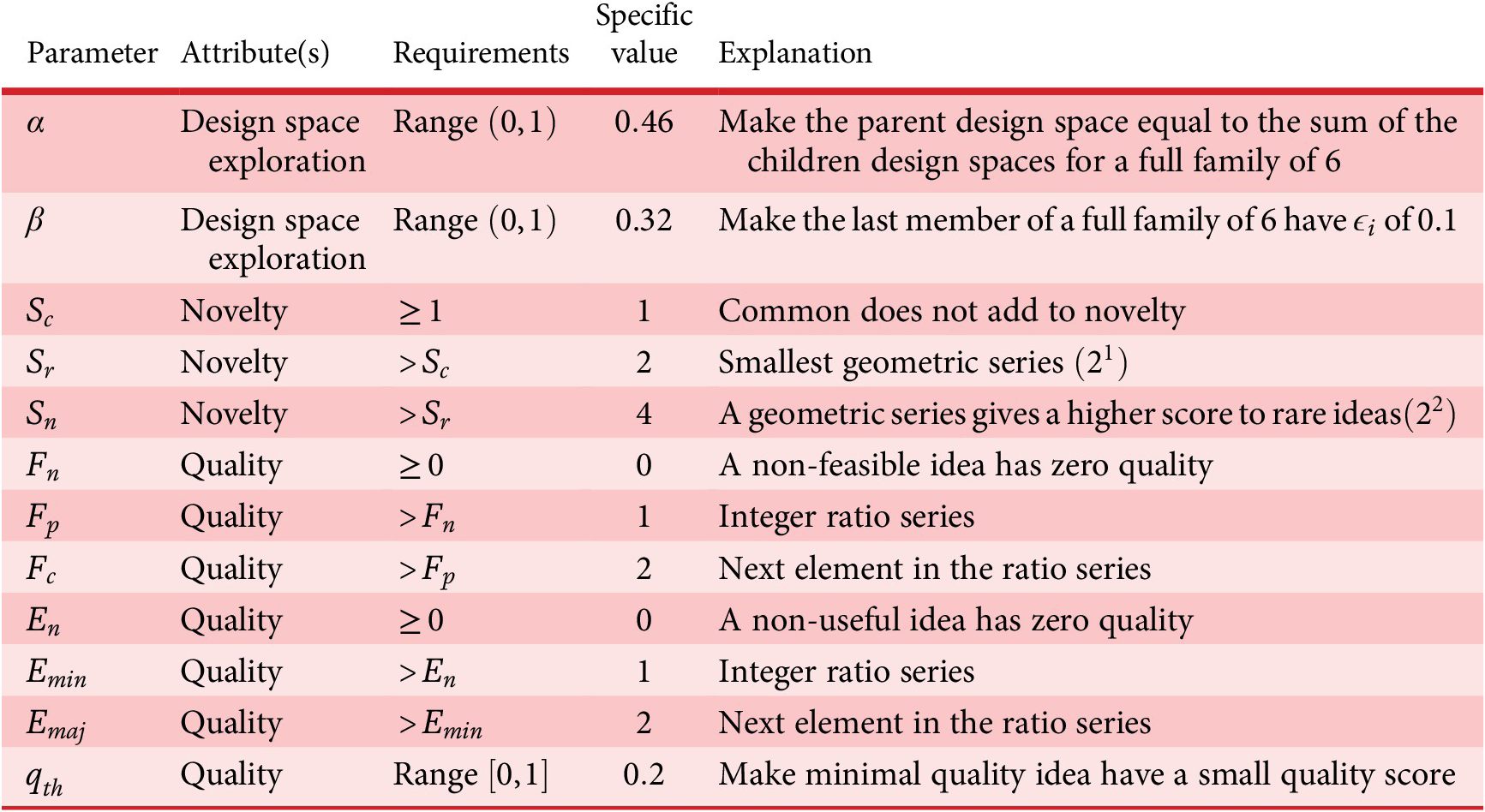
12.1. Design space exploration parameters
There are two parameters that govern
 $ {X}_{i,l} $
, the amount of design space explored by an idea that is member
$ {X}_{i,l} $
, the amount of design space explored by an idea that is member
 $ i $
in a family at level
$ i $
in a family at level
 $ l $
:
$ l $
:
 $ \alpha $
and
$ \alpha $
and
 $ \beta $
.
$ \beta $
.
 $ \alpha $
is the minimum fraction of
$ \alpha $
is the minimum fraction of
 $ {\Omega}_l $
that can be explored by an idea at level
$ {\Omega}_l $
that can be explored by an idea at level
 $ l $
. In addition, the recurrence relation in Eq. 10 shows that as the idea level increases by one,
$ l $
. In addition, the recurrence relation in Eq. 10 shows that as the idea level increases by one,
 $ {\Omega}_l $
grows by a factor of
$ {\Omega}_l $
grows by a factor of
 $ 1/\alpha $
. The equations have been defined so that as long as both
$ 1/\alpha $
. The equations have been defined so that as long as both
 $ \alpha $
and
$ \alpha $
and
 $ \beta $
lie between 0 and 1, the axioms will hold. There must be some additional considerations in selecting values for
$ \beta $
lie between 0 and 1, the axioms will hold. There must be some additional considerations in selecting values for
 $ \alpha $
and
$ \alpha $
and
 $ \beta $
.
$ \beta $
.
We have chosen two characteristics of design space that we believe are reasonable and allow us to find specific values for
 $ \alpha $
and
$ \alpha $
and
 $ \beta $
. The first is the concept of a “full” family. Although there is technically no limit to the number of family members, in practice, we believe the benefit of adding more family members drops off significantly as the number of members increases. As shown in Equation 8, the fraction for a family member is
$ \beta $
. The first is the concept of a “full” family. Although there is technically no limit to the number of family members, in practice, we believe the benefit of adding more family members drops off significantly as the number of members increases. As shown in Equation 8, the fraction for a family member is
 $ \alpha $
plus a bonus fraction
$ \alpha $
plus a bonus fraction
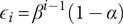 $ {\epsilon}_i={\beta}^{i-1}\left(1-\alpha \right) $
that decreases exponentially with
$ {\epsilon}_i={\beta}^{i-1}\left(1-\alpha \right) $
that decreases exponentially with
 $ i $
. Figure 7 shows how
$ i $
. Figure 7 shows how
 $ {\epsilon}_i $
varies with
$ {\epsilon}_i $
varies with
 $ i $
and
$ i $
and
 $ \beta $
.
$ \beta $
.
The variation in
 $ {\epsilon}_i $
with family member for multiple values of
$ {\epsilon}_i $
with family member for multiple values of
 $ \beta $
. The smaller the value of
$ \beta $
. The smaller the value of
 $ \beta $
, the more quickly the value of
$ \beta $
, the more quickly the value of
 $ {\epsilon}_i $
drops. A family can be considered full when the value of
$ {\epsilon}_i $
drops. A family can be considered full when the value of
 $ {epsilon}_i $
drops below a user-chosen value of
$ {epsilon}_i $
drops below a user-chosen value of
 $ {\epsilon}_{i_f} $
.
$ {\epsilon}_{i_f} $
.

A full family will have
 $ {i}_f $
members, and the value of
$ {i}_f $
members, and the value of
 $ {\epsilon}_{i_f} $
should be small.
$ {\epsilon}_{i_f} $
should be small.
 $ \beta $
can be calculated from
$ \beta $
can be calculated from
 $ {i}_f $
and
$ {i}_f $
and
 $ {\epsilon}_{i_f} $
.
$ {\epsilon}_{i_f} $
.
 $$ \beta ={\epsilon}_{i_f}^{1/\left({i}_f-1\right)} $$
Table 3 shows the values of
 $ \beta $
for various values of
$ \beta $
for various values of
 $ {i}_f $
and
$ {i}_f $
and
 $ {\epsilon}_{i_f} $
. We chose
$ {\epsilon}_{i_f} $
. We chose
 $ {i}_f=3 $
and
$ {i}_f=3 $
and
 $ {\epsilon}_{i_f}=0.1 $
which gives a value of
$ {\epsilon}_{i_f}=0.1 $
which gives a value of
 $ \beta =0.32 $
.
$ \beta =0.32 $
.
Values of
 $ \beta $
that give the specified value of
$ \beta $
that give the specified value of
 $ {\epsilon}_{i_f} $
at a given family size
$ {\epsilon}_{i_f} $
at a given family size
 $ {i}_f $

The second characteristic of design space that we believe is reasonable is that
 $ \alpha $
should be chosen such that the total design space occupied by a full family of size
$ \alpha $
should be chosen such that the total design space occupied by a full family of size
 $ {i}_f $
is equal to the design space occupied by the parent. The total design space occupied by a family at level
$ {i}_f $
is equal to the design space occupied by the parent. The total design space occupied by a family at level
 $ l $
is given by
$ l $
is given by
 $ {f}_t{\Omega}_l $
, where
$ {f}_t{\Omega}_l $
, where
 $ {f}_t $
is defined in Equation 9. The maximum design space occupied by the parent of a family at level
$ {f}_t $
is defined in Equation 9. The maximum design space occupied by the parent of a family at level
 $ l $
is
$ l $
is
 $ {\Omega}_{l+1} $
. Thus
$ {\Omega}_{l+1} $
. Thus
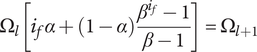 $$ {\Omega}_l\left[{i}_f\alpha +\left(1-\alpha \right)\frac{\beta^{i_f}-1}{\beta -1}\right]={\Omega}_{l+1} $$
Dividing both sides of the equation by
 $ {\Omega}_{l+1} $
and applying Equation 10, we obtain
$ {\Omega}_{l+1} $
and applying Equation 10, we obtain
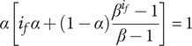 $$ \alpha \left[{i}_f\alpha +\left(1-\alpha \right)\frac{\beta^{i_f}-1}{\beta -1}\right]=1 $$
This equation can be solved numerically to determine a value for
 $ \alpha $
. Table 4 shows values of
$ \alpha $
. Table 4 shows values of
 $ \beta $
and
$ \beta $
and
 $ \alpha $
for
$ \alpha $
for
 $ {\epsilon}_{i_f}=0.1 $
and various values of
$ {\epsilon}_{i_f}=0.1 $
and various values of
 $ {i}_f $
.
$ {i}_f $
.
Values of
 $ \beta $
and
$ \beta $
and
 $ \alpha $
that give equal design space for the parent and the children for
$ \alpha $
that give equal design space for the parent and the children for
 $ {\epsilon}_{i_f}=0.1 $
and various values of
$ {\epsilon}_{i_f}=0.1 $
and various values of
 $ {i}_f $
. Values of
$ {i}_f $
. Values of
 $ \alpha $
and
$ \alpha $
and
 $ \beta $
have been rounded to two decimal places
$ \beta $
have been rounded to two decimal places

We note that in many early-stage design trees, families are relatively small. We also wish to keep
 $ \alpha $
between 0.4 and 0.5, to keep
$ \alpha $
between 0.4 and 0.5, to keep
 $ {\Omega}_l $
from increasing too rapidly. We chose a full family size of
$ {\Omega}_l $
from increasing too rapidly. We chose a full family size of
 $ {i}_f=3 $
and
$ {i}_f=3 $
and
 $ {\epsilon}_{i_f}=0.1 $
, which gives us
$ {\epsilon}_{i_f}=0.1 $
, which gives us
 $ \beta =0.32 $
and
$ \beta =0.32 $
and
 $ \alpha =0.46 $
. Other values for
$ \alpha =0.46 $
. Other values for
 $ {i}_f $
and
$ {i}_f $
and
 $ {\epsilon}_{i_f} $
could be chosen, leading to different calculated values for
$ {\epsilon}_{i_f} $
could be chosen, leading to different calculated values for
 $ \beta $
and
$ \beta $
and
 $ \alpha $
.
$ \alpha $
.
12.2. Novelty parameters
There are three parameters that must be chosen to calculate novelty scores using our method. These are
 $ {S}_c $
,
$ {S}_c $
,
 $ {S}_r $
and
$ {S}_r $
and
 $ {S}_n $
, the numerical scores for a common, rare and never-seen idea. We choose
$ {S}_n $
, the numerical scores for a common, rare and never-seen idea. We choose
 $ {S}_c=1 $
, because we multiply two scores together to obtain the novelty points, and 1 is the multiplicative identity.
$ {S}_c=1 $
, because we multiply two scores together to obtain the novelty points, and 1 is the multiplicative identity.
We chose to use a geometric series for the values of
 $ {S}_c $
,
$ {S}_c $
,
 $ {S}_r $
and
$ {S}_r $
and
 $ {S}_n $
in order to raise the score of rare ideas. We chose to use the smallest integral geometric series of
$ {S}_n $
in order to raise the score of rare ideas. We chose to use the smallest integral geometric series of
 $ {2}^n $
giving scores of 1, 2 and 4 for
$ {2}^n $
giving scores of 1, 2 and 4 for
 $ {S}_c $
,
$ {S}_c $
,
 $ {S}_r $
and
$ {S}_r $
and
 $ {S}_n $
, respectively.
$ {S}_n $
, respectively.
12.3. Quality parameters
There are seven parameters to be chosen to calculate quality scores:
 $ {F}_n $
,
$ {F}_n $
,
 $ {F}_p $
,
$ {F}_p $
,
 $ {F}_c $
,
$ {F}_c $
,
 $ {E}_n $
,
$ {E}_n $
,
 $ {E}_{min} $
,
$ {E}_{min} $
,
 $ {E}_{maj} $
and
$ {E}_{maj} $
and
 $ {q}_{th} $
. An idea that is infeasible has zero quality, so
$ {q}_{th} $
. An idea that is infeasible has zero quality, so
 $ {F}_n=0 $
. Similarly, an idea that has no effect or a negative effect on meeting requirements has zero quality, so
$ {F}_n=0 $
. Similarly, an idea that has no effect or a negative effect on meeting requirements has zero quality, so
 $ {E}_n $
= 0. Equal weighting of feasibility and effectiveness when determining quality requires
$ {E}_n $
= 0. Equal weighting of feasibility and effectiveness when determining quality requires
 $ {F}_p={E}_{min} $
and
$ {F}_p={E}_{min} $
and
 $ {F}_c={E}_{maj} $
. For simplicity, we choose a ratio scale starting at 0 and integer values, which leads to
$ {F}_c={E}_{maj} $
. For simplicity, we choose a ratio scale starting at 0 and integer values, which leads to
 $ {F}_p={E}_{min}=1 $
and
$ {F}_p={E}_{min}=1 $
and
 $ {F}_c={E}_{maj}=2 $
. Note that because of the normalization found in Equation 36, the score is insensitive to the values chosen, as long as the scale is a ratio scale.
$ {F}_c={E}_{maj}=2 $
. Note that because of the normalization found in Equation 36, the score is insensitive to the values chosen, as long as the scale is a ratio scale.
 $ {q}_{th} $
is chosen to establish the minimum quality level that can be considered to have a non-zero quality. There are four possible idea quality scores
$ {q}_{th} $
is chosen to establish the minimum quality level that can be considered to have a non-zero quality. There are four possible idea quality scores
 $ q $
: 0, 0.25, 0.5 and 1. A score of 0 is given to an idea that is infeasible or will have no impact or a negative impact on meeting requirements. Such ideas are not quality ideas, so
$ q $
: 0, 0.25, 0.5 and 1. A score of 0 is given to an idea that is infeasible or will have no impact or a negative impact on meeting requirements. Such ideas are not quality ideas, so
 $ {q}_{th}>0 $
. A score of 0.25 is given to an idea that is possibly feasible and will have a minor positive impact on meeting requirements. Such ideas are quality ideas, but not high-quality ideas. If
$ {q}_{th}>0 $
. A score of 0.25 is given to an idea that is possibly feasible and will have a minor positive impact on meeting requirements. Such ideas are quality ideas, but not high-quality ideas. If
 $ {q}_{th}\ge 0.25 $
, these ideas would have
$ {q}_{th}\ge 0.25 $
, these ideas would have
 $ {Q}_E=0 $
, which means
$ {Q}_E=0 $
, which means
 $ {q}_{th}<0.25 $
. The smaller the value of
$ {q}_{th}<0.25 $
. The smaller the value of
 $ {q}_{th} $
, the higher the value of
$ {q}_{th} $
, the higher the value of
 $ {Q}_E $
for an idea with the minimum non-zero quality rating. A choice of
$ {Q}_E $
for an idea with the minimum non-zero quality rating. A choice of
 $ {q}_{th}=0.2 $
gives an idea of major impact or certainly feasible a
$ {q}_{th}=0.2 $
gives an idea of major impact or certainly feasible a
 $ {Q}_E $
score six times that of one with the minimum non-zero quality rating, while an idea having both major impact and certain feasibility has a
$ {Q}_E $
score six times that of one with the minimum non-zero quality rating, while an idea having both major impact and certain feasibility has a
 $ {Q}_E $
score 16 times higher. We believe this gives an appropriate weight to truly high-quality ideas.
$ {Q}_E $
score 16 times higher. We believe this gives an appropriate weight to truly high-quality ideas.
13. Comparison with SVS metrics
Since its publication in 2003, the SVS method has been the de facto standard for evaluating idea sets that are placed in genealogy trees. Thus, a comparison of the axiomatic method proposed here with SVS is warranted. We will first consider quantity and variety, since these two metrics do not require evaluation of individual ideas; they are based solely on the tree structure.
13.1. Quantity and variety
To compare our method with the SVS method, we will use a tree that is modified from figure 4 in Shah et al. (Reference Shah, Smith and Vargas-Hernandez2003), shown in Figure 8. The SVS tree in part (a) has four levels, with level 1 at the top and level 4 at the bottom. A box at a given level represents an idea at that level that can be used to solve the problem. The number in the box shows the number of design solutions that use the referenced idea as part of their design. The numbers on the branches indicate the contribution of the branch to the sum
 $ {b}_k $
. The SVS weights of the four levels are shown as
$ {b}_k $
. The SVS weights of the four levels are shown as
 $ S1=10 $
,
$ S1=10 $
,
 $ S2=6 $
,
$ S2=6 $
,
 $ S3=3 $
and
$ S3=3 $
and
 $ S4=1 $
.
$ S4=1 $
.
A comparison of quantity and variety for a design tree evaluated by (a) the SVS method, and (b) the axiom-based method proposed in this paper.
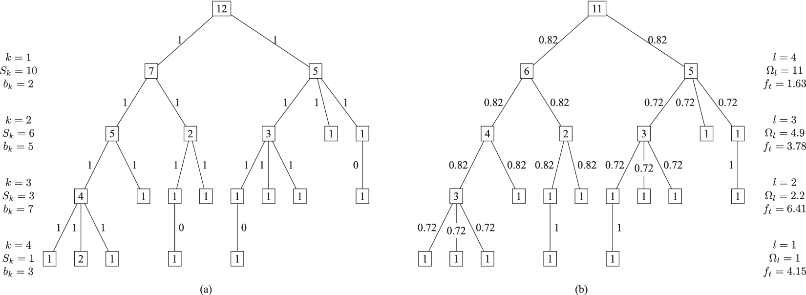
SVS quantity is calculated for each box by summing the numbers in the children of the box. The number in the top box represents the total quantity of ideas in the tree, so
 $ n=12 $
.
$ n=12 $
.
SVS variety is calculated as
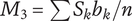 $ {M}_3=\sum {S}_k{b}_k/n $
:
$ {M}_3=\sum {S}_k{b}_k/n $
:
 $$ {M}_3=\left(1\cdot 3+3\cdot 7+6\cdot 5+10\cdot 2\right)/12=6.17 $$
Note that the
 $ n $
in the denominator means that an average variety is being calculated, so reducing the idea count by eliminating a low-variety idea can raise the variety score, thus violating Axiom V-1.
$ n $
in the denominator means that an average variety is being calculated, so reducing the idea count by eliminating a low-variety idea can raise the variety score, thus violating Axiom V-1.
The tree shown in part (b) also has four levels, but level 1 is the lowest level, and level 4 is the highest level. The numbers in the boxes are the branch quantity
 $ {U}_B $
for the branch headed by the box. The numbers are almost the same as SVS, but the second box from the left on the lowest level has 1 in the axiom-based tree, where the SVS tree has 2. This is because we consider only unique ideas, and two ideas that cannot be distinguished at the lowest level of the tree cannot both be unique. Thus, there is duplication, and we count only a single idea.
$ {U}_B $
for the branch headed by the box. The numbers are almost the same as SVS, but the second box from the left on the lowest level has 1 in the axiom-based tree, where the SVS tree has 2. This is because we consider only unique ideas, and two ideas that cannot be distinguished at the lowest level of the tree cannot both be unique. Thus, there is duplication, and we count only a single idea.
The weights for each level of the axiom-based tree are not arbitrary values of
 $ 1 $
,
$ 1 $
,
 $ 3 $
,
$ 3 $
,
 $ 6 $
and
$ 6 $
and
 $ 10 $
, but rather values of
$ 10 $
, but rather values of
 $ {\Omega}_l $
chosen to ensure the tree will meet Axiom TV-2:
$ {\Omega}_l $
chosen to ensure the tree will meet Axiom TV-2:
 $ 1 $
,
$ 1 $
,
 $ 1/\alpha $
,
$ 1/\alpha $
,
 $ 1/{\alpha}^2 $
and
$ 1/{\alpha}^2 $
and
 $ 1/{\alpha}^3 $
, which for a value of
$ 1/{\alpha}^3 $
, which for a value of
 $ \alpha =0.46 $
are
$ \alpha =0.46 $
are
 $ 1 $
,
$ 1 $
,
 $ 2.2 $
,
$ 2.2 $
,
 $ 4.9 $
and
$ 4.9 $
and
 $ 11 $
.
$ 11 $
.
In contrast with the SVS method, the numbers on the branches vary with the number of family members. The more family members, the lower the number on each branch. The numbers on the branches are the
 $ {f}_a $
values for the idea at the bottom of the branch. The total fraction for the level is
$ {f}_a $
values for the idea at the bottom of the branch. The total fraction for the level is
 $ {f}_{t_l} $
. The total variety is
$ {f}_{t_l} $
. The total variety is
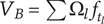 $ {V}_B=\sum {\Omega}_l{f}_{t_l} $
:
$ {V}_B=\sum {\Omega}_l{f}_{t_l} $
:
 $$ {V}_B=1\cdot 4.15+2.2\cdot 6.41+4.9\cdot 3.78+11\cdot 1.63=54.7 $$
Note that one cannot directly compare the variety scores from SVS and axiom-based aggregation, because they have a different normalization. Future work is planned on developing a normalized variety score that meets all of the axioms.
13.2. Novelty
It is difficult to directly compare the novelty scores for the SVS method and axiom-based aggregation. Both methods calculate an element novelty at a level of the tree, including a novelty score and a weighting parameter. The novelty scores are determined so differently in the two methods as to prevent direct comparison. The weighting functions are chosen by the rater in the SVS method and are determined by the area of design space explored by the idea in the axiomatic method.
SVS add the element novelties for the elements in a design solution to obtain a solution novelty. SVS give no means of measuring set novelty in the 2003 paper. Later work by Shah and Vargas-Hernandez alludes to using average solution novelty or best solution novelty. Axiom-based aggregation adds the element novelties for each element in the tree to give a total set novelty that accounts for each idea’s location in the tree (or, how much the design space has been expanded).
Where multiple design solutions share a tree element, the SVS average novelty will include the novelty of that element once for each solution. Axiom-based aggregation only adds the novelty of that element once.
13.3. Quality
SVS calculate an idea quality score at a given level of the tree as a weighted sum of the qualities of all individual functions needed at that level. It then multiplies the idea quality score by the weight of that level to obtain an element quality score. The element quality scores for a design alternative are then summed to give an alternative score. The set quality is the sum of the alternative qualities divided by the number of alternatives and the sum of function weights. Thus, the set quality reflects an average quality and can easily violate the quality axioms.
Axiom-based aggregation calculates an idea quality for each idea. There is no weighting for the levels, as quality does not appear to us to be related to the amount of design space explored by an idea. The element quality is determined from the idea quality by including the threshold quality for the tree, given by Equation 37. There is no increased weighting for quality scores at higher levels of the tree. The set quality score does increase more for a quality idea at a higher level of the tree because the branch quantity is larger at higher levels of the tree (see Equation 38). The set quality meets the axioms in all cases.
14. Mechanics of evaluation
With four attributes to evaluate and aggregation of individual scores for numerous ideas, the evaluation of an idea set can be challenging. Typically, there will be a large number of ideas to evaluate (in our experiments, often about 150 per team, and 10–12 teams). These ideas must be evaluated on their merits, placed into a tree and then tree-based aggregation functions must be evaluated. With the large number of equations involved in these calculations, the task is daunting if the calculations are carried out manually. Therefore, automated tools have been developed to support this evaluation process.
With the software tools available, the following, more manageable steps must be completed by an evaluator.
-
1. Place the ideas in a design tree
-
(a) Decide the level of the tree to which an idea belongs. In the case of our OPED trees, this means deciding whether the idea is a principle, an embodiment or a detail.
-
(b) For each idea, choose or create an appropriate parent. Each detail must have a parent embodiment. Each embodiment must have a parent principle. Each principle must have a parent objective. If the parents do not exist in the tree, they must be added.
-
-
2. Evaluate the individual ideas in the tree
-
(a) For each idea element, determine the Feasibility and Effectiveness rating. There are three distinct levels for each of these attributes.
-
(b) For each idea element, do the following:
-
i. Determine the prevalence rating Common, Rare or Never for the idea in the current design context
-
ii. Seek to identify another context where a similar idea is used to achieve a similar kind of result
-
iii. If another context is identified, determine the prevalence rating common, rare or never for the similar idea in the other context.
-
-
The design tree can be created by a single evaluator or by a team of evaluators working together. Once the tree is created, closely related ideas will be grouped together, which enhances consistency when rating the ideas. Different evaluators can independently rate the ideas to provide measures of repeatability in the evaluations. The idea evaluations are relatively coarse evaluations, which expedites the process.
When the tree is created, and the idea evaluations are complete, the software tools will calculate elements and set properties for quantity, quality, variety and novelty, and will create tree diagrams showing the tree and the attribute scores. With the provided tools, the calculations are easily performed, repeatable, and auditable by manually verifying any element or branch score in the tree.
A detailed description of the use of the tools is found in the appendix. The software tools are freely available for downloading at Sorensen et al. (Reference Sorensen, Mattson, Anderson and Ashworth2023).
15. Example evaluated tree
To demonstrate how the process works, we show an evaluated .csv file and a simple evaluated tree for an ideation set. These data were extracted from an ideation experiment on the topic of preventing disease spread through air travel. A complete tree containing 82 ideas is found in the supplemental materials. In this section, we present only 13 ideas related to the principle of Advertisement or Public Relations.
The .csv file containing the data is shown in Figure 9. The idea generated by the team is in the column Idea. The level of the idea is in the column Level (D, E or P). The principle, embodiment, and – if applicable – detail are shown in the principle, embodiment and detail columns, respectively. The evaluators’ ratings of feasibility and effectiveness are in the columns Feasibility and Impact, respectively. The automatically assigned scores for F, E, and Quality are in the respective columns. The novelty responses 1 through 4 were entered by the rater in the respective columns (the columns for responses 2 and 3 are left blank, as they do not affect the novelty rating). The point values
 $ {P}_d $
,
$ {P}_d $
,
 $ {P}_o $
and
$ {P}_o $
and
 $ P $
, as well as the novelty rating,
$ P $
, as well as the novelty rating,
 $ n $
are automatically calculated. Thus, once the tree is created, the rater needs only to enter four values for each idea (the values in the shaded columns) to prepare for tree creation and evaluation.
$ n $
are automatically calculated. Thus, once the tree is created, the rater needs only to enter four values for each idea (the values in the shaded columns) to prepare for tree creation and evaluation.
Excerpt of a .csv file from the evaluation of a sample ideation set on the topic of “Preventing Disease Spread Through Air Travel.” In this excerpt, only 13 ideas are shown that relate to the Principle of “Advertisement or Public Relations.”
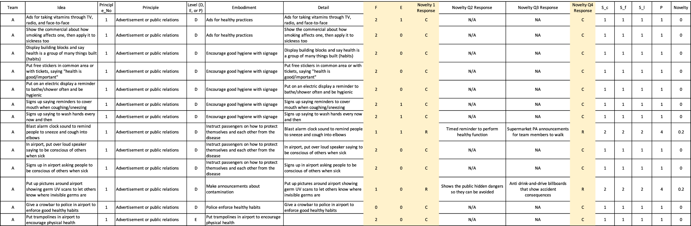
A single element of the design tree is shown in Figure 15. As with all elements in the tree, there are four rows of information. The first row is the title of the element, and contains four pieces of information:
-
1. The kind of element, either an idea element created by the team or an organizational element added by the evaluator.
-
2. The tree level of the element.
-
3. An identifying number for easy reference.
-
4. A brief description of the idea.
The second row lists the idea properties, which are calculated irrespective of the tree location. The two idea properties are idea novelty
 $ n $
and idea quality
$ n $
and idea quality
 $ q $
. Both have possible values between 0 and 1, with higher values corresponding to higher quality and novelty.
$ q $
. Both have possible values between 0 and 1, with higher values corresponding to higher quality and novelty.
The third row lists the element properties, which include the tree location in their calculation. There are four element properties:
-
1. Uniqueness
$ u $
, which has a value of 0 or 1. -
2. Element novelty
$ {N}_E $
, which has a value between 0 and 1. -
3. Element variety
$ {V}_E $
, a positive value that depends on the tree level and the size of the family. -
4. Element quality
$ {Q}_E $
, which has a value between 0 and 1.


The fourth row lists the branch properties, which are the aggregated properties for the subtree with the element as the root node. There are four branch properties:
-
1. The branch quantity
$ {U}_B $
. -
2. The branch novelty
$ {N}_B $
. -
3. The branch variety
$ {V}_B $
. -
4. The branch quality
$ {Q}_B $
.


Figure 10 shows the design tree of all ideas implementing the principle P1: Advertisement or Public Relations. Although this figure is difficult to read in printed form, it shows the overall layout of the design tree. Relevant regions of the tree will be shown in detail in subsequent figures.
A sample tree with calculated quality, quantity, variety and novelty. This figure shows the relationships; the following figures allow interpreting the data. This figure is intended to communicate the overall structure of this subtree.

There are 12 details, six embodiments and one principle in this subtree. The number of details per embodiment ranged from zero to five. There were 13 unique ideas in the set. Only four ideas had a quality exceeding the threshold of 0.2. Only two had a novelty greater than zero.
The set has a quantity of 13, a variety of 22.27, a novelty of 0.4 and a quality of 1.19.
Figure 11 shows embodiment E1 and its two related details, D1 and D2.
A sample tree with calculations (part A). This figure shows a single organizational embodiment with its details. The branch properties are equal to the element properties plus the sum of the descendant branch properties.
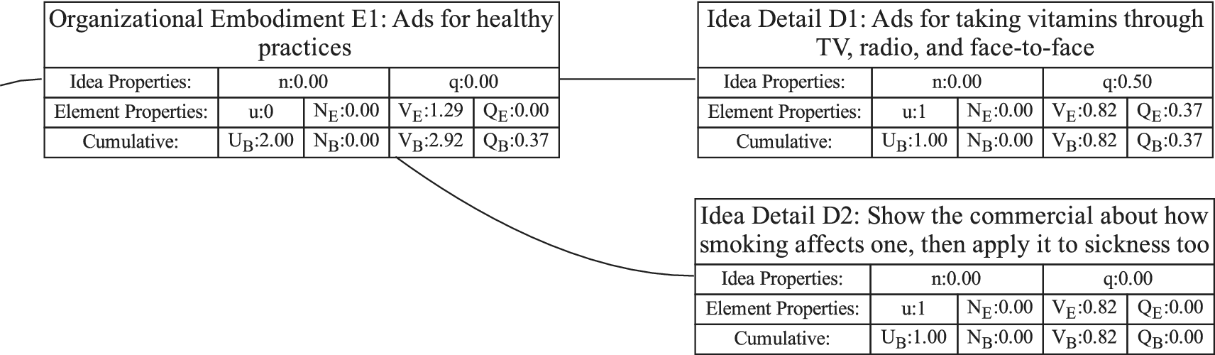
Because E1 is an organizational element, its idea novelty is 0. Similarly, its quality is set to zero without evaluation.
E1 has children, so
 $ u=0 $
. Because the idea novelty is 0, the element novelty is 0. The element variety is 1.29. The element quality is 0.
$ u=0 $
. Because the idea novelty is 0, the element novelty is 0. The element variety is 1.29. The element quality is 0.
The branch quantity is
 $ 2.0 $
(the sum of the branch quantities for the children). The branch novelty is
$ 2.0 $
(the sum of the branch quantities for the children). The branch novelty is
 $ 0 $
(the sum of element novelty plus the branch novelties for the children). The branch variety is
$ 0 $
(the sum of element novelty plus the branch novelties for the children). The branch variety is
 $ 1.29+0.82+0.82=2.92 $
. The branch quality is
$ 1.29+0.82+0.82=2.92 $
. The branch quality is
 $ 0+0.37+0=0.37 $
.
$ 0+0.37+0=0.37 $
.
Details D1 and D2, like all details, have
 $ \Omega =1 $
. There are two members of their family. Both ideas were evaluated to have
$ \Omega =1 $
. There are two members of their family. Both ideas were evaluated to have
 $ n=0 $
. D1 has an idea quality
$ n=0 $
. D1 has an idea quality
 $ q=0.5 $
. D2 has an idea quality
$ q=0.5 $
. D2 has an idea quality
 $ q=0 $
. Both elements are leaf elements, so
$ q=0 $
. Both elements are leaf elements, so
 $ u=1 $
. Because
$ u=1 $
. Because
 $ n=0 $
for both elements,
$ n=0 $
for both elements,
 $ {N}_E=0 $
for both elements.
$ {N}_E=0 $
for both elements.
 $ {V}_E=0.82 $
for both elements.
$ {V}_E=0.82 $
for both elements.
 $ {Q}_E=0.37 $
for element D1 and
$ {Q}_E=0.37 $
for element D1 and
 $ 0 $
for element D2. Because there are no children, the branch quantity, novelty, variety and quality are equal to the element quantity, novelty, variety and quality.
$ 0 $
for element D2. Because there are no children, the branch quantity, novelty, variety and quality are equal to the element quantity, novelty, variety and quality.
Figure 12 shows embodiment E2 and all of its underlying details. None of these ideas is novel. Details D3, D4 and D5 have a quality
 $ q=0 $
. Details D6 and D7 have a quality
$ q=0 $
. Details D6 and D7 have a quality
 $ q=0.5 $
.
$ q=0.5 $
.
A sample tree with calculations (part B). This figure shows a single organizational embodiment with its details. The branch properties are equal to the element properties plus the sum of the descendant branch properties.

Figure 13 shows embodiment E3 with its children’s details. Idea D8 has novelty
 $ n=0.2 $
and quality
$ n=0.2 $
and quality
 $ q=0.25 $
. This leads to an element novelty of
$ q=0.25 $
. This leads to an element novelty of
 $ {N}_E=0.2 $
and an element quality of
$ {N}_E=0.2 $
and an element quality of
 $ {Q}_E=0.06 $
.
$ {Q}_E=0.06 $
.
A sample tree with calculations (part C). This figure shows a single organizational embodiment with its details.
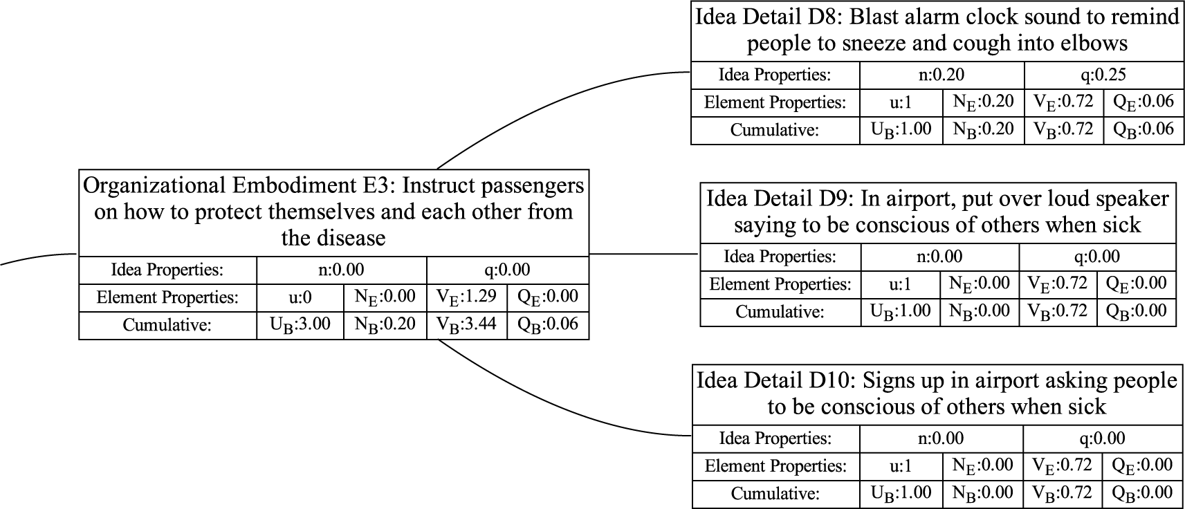
Figure 14 shows embodiments E4 through E6. E4 and E5 are organizational embodiments and each has one child. E6 is an idea embodiment with no children, so it has
 $ u=1 $
.
$ u=1 $
.
A sample tree with calculations (part D). This figure shows three embodiments, two of which are organizational elements, while the third is an idea element. The first two embodiments have an idea novelty
 $ n=0 $
because they are organizational elements. They have
$ n=0 $
because they are organizational elements. They have
 $ u=0 $
because the parent idea is shared with all of the children. The third embodiment has
$ u=0 $
because the parent idea is shared with all of the children. The third embodiment has
 $ n=0 $
because the idea was evaluated to have zero novelty and
$ n=0 $
because the idea was evaluated to have zero novelty and
 $ u=1 $
because it has no children.
$ u=1 $
because it has no children.

Figure 15 shows principle P1. As an organizational principle, it has a novelty of 0 and its quality is not evaluated, so
 $ {Q}_E=0 $
. The branch quantity, quality, novelty and variety are given by the sum of the respective branch properties of the children plus the respective element properties for P1.
$ {Q}_E=0 $
. The branch quantity, quality, novelty and variety are given by the sum of the respective branch properties of the children plus the respective element properties for P1.
A sample tree with calculations (part E). This figure shows the principle that is responsible for all the quantity, novelty, variety and quality in its branch. Note that the branch scores
 $ {U}_B $
,
$ {U}_B $
,
 $ {N}_B $
,
$ {N}_B $
,
 $ {V}_B $
. and
$ {V}_B $
. and
 $ {Q}_B $
are the sum of the scores for the element plus the branch scores of its children (the embodiments in parts A through D).
$ {Q}_B $
are the sum of the scores for the element plus the branch scores of its children (the embodiments in parts A through D).

Figure 16 shows the tree properties for this subtree. The objective is not an idea, so it has neither idea nor element properties. The tree properties are the branch properties of this element. The branch properties are equal to the descendant properties, because all element properties are zero.
A sample tree with calculations (part F). This figure shows the objective for this design exercise. This is an objective, rather than a design idea, so
 $ \Omega =0 $
. There are no idea properties or element properties. Because there is only one principle in this tree, the cumulative properties for the set are equal to the cumulative properties of the single principle.
$ \Omega =0 $
. There are no idea properties or element properties. Because there is only one principle in this tree, the cumulative properties for the set are equal to the cumulative properties of the single principle.
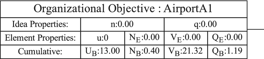
16. Discussion
We have demonstrated a method for calculating set quantity, quality, variety and novelty for sets of early stage ideas. This method is demonstrated to provide results consistent with the axioms we have created for how set aggregation functions should behave in order to encourage and reward best practices during ideation.
The quantity and quality methods have no undesirable characteristics of which we are aware. The sum of quality exceeding a threshold recognizes both the number of high-quality ideas and the relative quality of the ideas.
The aggregation functions for all attributes have been demonstrated to be consistent with the axioms. However, there is no absolute scale for determining the variety and novelty of an idea set. While the metrics of two sets can be compared to determine which of the sets is higher in novelty and variety, the metrics cannot yet be used to say whether a set has “enough” novelty or variety. Future work is needed to better understand the meaning of these specific metrics in absolute terms. This could potentially help an engineering manager and/or a design team decide whether it is time to move on from the ideation stage.
Both the variety and novelty scores are correlated with the quantity of ideas. Common methods to decouple from the quantity, such as calculating average novelty or average quality, cannot be used because they fail to meet the axioms. It would be desirable to develop variety and novelty scores that are less correlated with quantity.
The calculation methods have been used in multiple experiments to evaluate very large idea sets (over 2000 ideas) generated by large numbers of teams (more than 15) working on a common design problem. Although the evaluation work is challenging, it is feasible for an individual to complete. A set of 2000 ideas can be evaluated in less than 100 hours of working time.
We have also used multiple evaluators on these large sets. We have anecdotally observed an increase in variation with multiple raters (as would be expected), but our experiments have not allowed us to complete an effective statistical analysis of the effects of multiple evaluators.
Software infrastructure has been developed to support the evaluation. The software allows repeatable work to evaluate ideation results. Trees that display the individual element scores are automatically generated.
One limitation of the idea evaluation methods presented in this work is that they are dependent on tree-based methods. There is no inherent “perfect” tree structure, so different evaluators will have different trees. The effects of such differences on the idea set scores have not yet been evaluated and are left for future work.
Although the evaluations for quality and novelty are subjective, the evaluation is structured enough to allow the rating to be repeatable. The method used to complete the subjective evaluations places similar ideas in close proximity during the subjective evaluation, thus facilitating a consistent evaluation. Further work to quantify both interrater reliability and individual rater repeatability for these evaluation methods should be completed.
The evaluation methods involve answering simple questions. It might be interesting to explore the development of large language models (LLMs) that could answer these questions for a particular class of design ideas. Such a model might reduce the time necessary for the evaluation while simultaneously reducing variation in the results.
17. Conclusion
Axioms have been developed that define the ideal behavior of aggregation functions for quantity, variety, novelty and quality. These axioms are designed to ensure that the resulting scoring methods reflect best practices in ideation and appropriately reward preferred ideation behavior. In addition to the general axioms, specific axioms have been developed for idea sets organized into design trees.
The axioms provide a consistent way to examine the behavior of any proposed metric for the quality of an idea set. Set metrics that meet the axioms are demonstrably better than set metrics that fail to meet the axioms.
We have demonstrated that typical aggregation functions used in the literature for calculating properties of the idea sets can violate the axioms. In these cases, the aggregation functions provide less support for preferred ideation behavior.
When the aggregation methods for idea set properties follow the axioms, calculated set properties can be used to evaluate the quality of the ideation processes employed by the individual or team generating the ideas. These tools then support research into novel ideation methods.
Simple evaluation methods that are consistent with the literature and appropriate for use with large numbers of early-stage ideas have been developed. Software tools to support these evaluation methods were created and are made publicly available. These methods and tools have been demonstrated for use on sets containing thousands of ideas and have been found to be feasible for completing the evaluations in a reasonable time.
Additionally, software tools that calculate tree-based aggregation functions were created and are made publicly available. These tools automatically take the output of the ideation process, and evaluations of the quality and novelty for each idea, and calculate the set quality, quantity, novelty and variety using the axiom-based aggregation functions. This supports practical research in ideation methods.
Financial support
This research was funded in part by the United States Air Force Academy under Cooperative Research Agreements FA7000-21-2-0007.
A. Appendix: Software tools for calculating and displaying idea set metrics
Software for taking a list of ideas with evaluation data, calculating set metrics and generating trees to display the sets and the metric calculation information is available at Sorensen et al. (Reference Sorensen, Mattson, Anderson and Ashworth2023). In preparation for calculating the idea set scores, the evaluation worksheet should be sorted by team, then principle number, then embodiment, then detail. The list of evaluated ideas for each team should be copied to a separate worksheet. The team’s ideas should have the column labels from the ratings worksheet. The workbook has a macro “SaveAllTeams” that extracts the individual team data and saves it in a set of CSV files.
All saved team worksheets can be evaluated from a terminal window by executing the shell script process-CSVS-notectac.sh.
A single team worksheet can be processed from a terminal window by executing the shell script process-one-CSV-notectac.sh.
Alternatively, the file import-csv-notectac.py can be opened in a Python editor, the TreeName, ImportFile and ObjectiveName variables edited to match the data being analyzed, and the Python program executed.
The set quantity, variety, novelty and quality will be displayed on the output window if you are running import-csv.py or process-one-CSV-notectac.sh. If you are using process-CSVS-notectac.sh, you will get a screen full of data that can be copied to a text file, or you can use shell redirection to have the text file created automatically.
A1. Create set displays (optional)
As the set scores are calculated, a series of graphviz input files is created that can be used to display the idea trees. If graphviz is installed on your system, a pdf image of the tree can be created with the command.
dot -OP -Tpdf <filename>.dot.
If importTotalCSVs.sh or process-one-CSV-notectac.sh is executed, the following pdf images will be created automatically.
-
• The *Plain.dot.pdf files will have only the idea names (similar to Figure 4).
-
• The *Simple.dot.pdf files will list the idea novelty and quality, the element uniqueness, novelty, variety and quality, and the branch quantity, novelty, variety and quality (similar to Figure 10).
-
• The *Diagnostic.dot.pdf files will list all of the values necessary to calculate the idea, element and branch properties, along with the idea, element and branch properties (similar to Figure A2).
A2. Using the scoring workbook
A Microsoft Excel scoring workbook is used to facilitate the formation of the design tree, evaluating the novelty and quality of the ideas and calculating the element, branch and set quantity, novelty, variety and quality. This section describes how the workbook is used. Please have the workbook open on a computer while you read this section.
A3. Capturing the generated ideas
A written description of each of the ideas in the set is copied into the Idea column of the Ratings worksheet. This entry need not be a complete description; it serves only as a label to identify the idea for convenience in evaluation.
If the set includes the work of multiple teams (such as to evaluate the performance of different ideation methods), an identifier for the idea set from which the idea was taken is placed in the Team column of the worksheet. This allows the ideas to be sorted as a whole for easier evaluation and then separated by team after the evaluation is complete. It is helpful to have all ideas being evaluated in a single worksheet, rather than having separate worksheets for separate idea sets. If all ideas being evaluated are from a single team, it is not necessary to add a team identifier.
A4. Tree formation
Once the ideas are captured in the worksheet, a design tree is formed from the ideas. This involves assigning each idea to a level of the tree, assigning each embodiment or detail idea to a principle and assigning each detail idea to an embodiment.
A4.1. Assign a level to each idea
The tree level for each idea (principle, embodiment or detail) is determined and the corresponding code of P, E or D is placed in the Level column. If the idea is assigned as a detail, the idea text is automatically copied to the Detail column. If the idea is assigned as an embodiment, the idea text is automatically copied to the Embodiment column.
If the idea is assigned as a principle, the Embodiment column and the Detail column will both be left empty. If the principle is different from any previously defined principles, it should be added to the Principles worksheet and given a unique principle number. If it is essentially the same as one of the previous principles, it is given the number of the previous principle and either the idea name or the previous principle name should be changed so that both the previous principle and the current idea have the same name. The principle number from the Principles worksheet should be placed in the Principle_No column for the idea on the Ratings worksheet.
In columns D, E and F of the Principles worksheet, there are calculations for the total number of ideas and the number of ideas assigned to each principle. These are used to ensure that all ideas have been assigned a principle. To keep these formulas correct, you will need to copy the formula in column D down to each row that has a principle. If you choose not to use these calculations, it will not affect the scoring of the ideas.
A4.2. Creating the initial principle set
The set of principles chosen for inclusion in the design tree can have a significant impact on the tree. Therefore, we find it helpful to spend substantial effort to identify an initial principle set that will effectively cover most of the ideas in the tree. It is helpful to have multiple experienced raters collaborate in creating the initial principle set.
To create the initial set of principles, a large number of ideas (approximately 200) are selected from the ideation results. If the idea set is smaller than 200, all ideas are used. If the idea set is larger, a random selection is made to obtain about 200 ideas.
Each of the selected ideas is placed on a Post-it note or an index card; the notes are then placed on a large whiteboard, wall or tabletop. Working simultaneously, the raters place the idea cards in related groups. After a period of time, a stable arrangement of the cards will begin to appear. Each of the stable groups will then be labeled with a proposed principle. As proposed principles are written down, ideas may be moved to a different group. The proposed principles may be modified for clarity. Additional principles may be proposed as ideas are reorganized.
When the raters are satisfied that the set of proposed principles is effective for classifying the selected ideas, each of the principles is put into the Principles worksheet. The principle will have a principle number, a principle label and a description that clarifies the label.
The identified principles will be put in the Principles worksheet, along with a sequential principle number. Ideas will be assigned a principle number, rather than the text of a principle. This ensures that all ideas having the same principle use the same text to describe it.
When adding principles to the Principles worksheet, insert new rows above the indicated row on that worksheet, then place the principle on the new row. This will allow formulas that automatically populate the principles on the Ratings worksheet to work correctly.
A4.3. Assign a principle to each idea
Each of the ideas in the idea column is then assigned a principle number in the Principle_No column. The principle description is automatically copied into the Principle column. If two ideas are judged to be identical, the wording for both ideas should be made equivalent, which will cause the ideas to be considered the same idea by the tree-forming software. If the duplicate ideas are from a single team, keep only one of the duplicate ideas.
Some ideas may not have enough information to assign a principle. When this is the case, assign the principle number of 0. Before calculating the set scores, remove all ideas with principle number 0. The Ratings worksheet is then sorted by principle number, which means that all closely related ideas are grouped together.
A4.4. Assign an embodiment for each detail
For detail-level ideas, an embodiment is assigned by typing an embodiment description in the embodiment column. Where possible, existing embodiments should be used. It is best to use copy and paste with existing embodiments to avoid typing errors.
Every unique embodiment in the workbook should have a unique description, although it can be applied to many details. All appearances of the unique embodiment must be children of the same principle. If two different principles have embodiments with similar descriptions, be sure the embodiment descriptions are different enough to be obvious to the reader, in order to avoid confusion.
Design trees are improperly formed and will result in calculation errors if a particular embodiment is listed as a child of two different principles. As details are compared (and embodiments are created), if two detail ideas from a given team are found to be identical, one of the duplicates should be eliminated. If two detail ideas from different teams are found to be identical, leave both in the Ratings worksheet. Note that only idea elements have individual rows in the worksheet. Organizational Elements do not have their own row, so they will not be evaluated for quality or novelty.
A5. Evaluate quality
Once the tree is properly formed as described in the previous section, the quality and novelty of the ideas must be evaluated. In preparation for evaluating quality, it is generally best to do a three-level sort: first by principle number, second by embodiment, third by detail. This does a reasonable job of placing closely related ideas in proximity for the evaluation.
Evaluate each idea for feasibility as described in Idea Quality, and place the appropriate rating C, P or N in the Feasibility Rating column. Next, evaluate each idea for impact on meeting the design requirements as described in Idea Quality, and place the appropriate rating MAJ, MIN or N in the Impact Rating column. Formulas in the worksheet automatically calculate
 $ F $
,
$ F $
,
 $ E $
and
$ E $
and
 $ q $
quality based on these entries.
$ q $
quality based on these entries.
A6. Evaluate novelty
Evaluate each idea for novelty as described in “Evaluating Idea Novelty.” C, R or N should be placed in the Novelty 1 Response column for usage in the design context. If the response in step 1 is C, the Novelty 2 Response and Novelty 3 Response columns are left blank, and worksheet formulas place C in the Novelty 4 response column.
If the Novelty 1 Response is R or N, complete the Novelty 2 Response and Novelty 3 Response columns to identify the mechanism or technique of the idea and another context where a similar idea is used for this mechanism. Then, determine the prevalence of the idea used in the Novelty 3 response context and place C, R or N in the Novelty 4 response column. Formulas in the worksheet automatically calculate
 $ {P}_d $
,
$ {P}_d $
,
 $ {P}_o $
and
$ {P}_o $
and
 $ P $
based on Novelty 1 Response and Novelty 4 Response.
$ P $
based on Novelty 1 Response and Novelty 4 Response.
The total time to form the tree, evaluate the quality and evaluate the novelty ranges between 1 and 3 minutes per idea, depending on the skill of the rater.
A7. Calculate set scores
Once all the evaluations are completed, the set scores are calculated by software implementing the calculations described in this paper.
The total time to calculate the set scores from the imported data is on the order of 2 minutes or less.
A8. The diagnostic design tree
To allow validation of the automatic calculations in the tree-building software, a diagnostic design tree is created. Figure A1 shows a single element from a diagnostic tree. Figure A2 shows the diagnostic tree for the example evaluated tree in this paper.
An element from a diagnostic idea tree. This element contains all the values needed to check the calculations of tree, idea, element and branch properties, as described in the text.
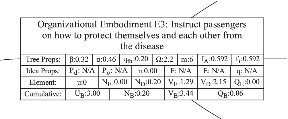
Each element in a diagnostic tree contains five rows. The first row is the title of the element, and contains four pieces of information:
-
1. The kind of element, either an idea element created by the team or an organizational element added by the evaluator.
-
2. The tree level of the element.
-
3. An identifying code for easy reference.
-
4. A brief description of the idea.
The second row lists the properties of the tee that will go into the calculation of element properties:
-
1.
$ \beta $
, the exponential parameter for reducing
$ {f}_i $
-
2.
$ \alpha $
, the basic design space fraction for an idea -
3.
$ {q}_{th} $
, the threshold quality score for the tree -
4.
$ \Omega $
, the nominal design space for an idea at this level of the tree, calculated from Equation 11 -
5.
$ m $
, the number of members in the element’s family -
6.
$ {f}_A $
, the fraction to be used in evaluating variety, calculated from Equation 13 -
7.
$ {f}_i $
, the fraction to be used in evaluating novelty, calculated from Equation 8.


The third row lists the idea properties along with the values that are used for the calculation of these properties:
-
1.
$ {P}_d $
, the novelty points for the idea in the design context -
2.
$ {P}_o $
, the novelty points for the idea in another context -
3.
$ n $
, the idea novelty calculated from
$ {P}_d $
and
$ {P}_o $
according to Equation 21 -
4.
$ F $
, the feasibility score for the idea -
5.
$ E $
, the effectiveness score for the idea -
6.
$ q $
, the idea quality calculated from
$ E $
and
$ F $
according to Equation 36.


The fourth row lists the element properties, along with values that are used for the calculation of these properties (Figures A3– A7).
-
1.
$ u $
, the uniqueness of the element, calculated from Equation 33 -
2.
$ {N}_E $
, the element novelty, calculated from Equation 23 -
3.
$ {N}_D $
, the novelty of the descendants of the element, calculated from Equation 25 -
4.
$ {V}_E $
, the element variety, calculated from Equation 14 -
5.
$ {V}_D $
, the variety of the descendants of the element, calculated from Equation 16 -
6.
$ {Q}_E $
, the element quality, calculated from Equation 37.


The fifth row lists the cumulative properties for the branch:
-
1.
$ {U}_B $
, the branch quantity, calculated from Equation 35 -
2.
$ {N}_B $
, the branch novelty, calculated from Equation 26 -
3.
$ {V}_B $
, the branch variety, calculated from Equation 15 -
4.
$ {Q}_B $
, the branch quality, calculated from Equation 38.


A diagnostic tree with calculated quality, quantity, variety and novelty. This figure shows the relationships; the following figures allow interpreting the data. This figure is intended to communicate the overall structure of this subtree.

Subtree A: One embodiment and two details of the diagnostic tree.
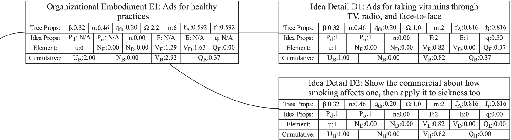
Subtree B: One embodiment and five details of the diagnostic tree.

Subtree C: One embodiment and three details of the diagnostic tree.
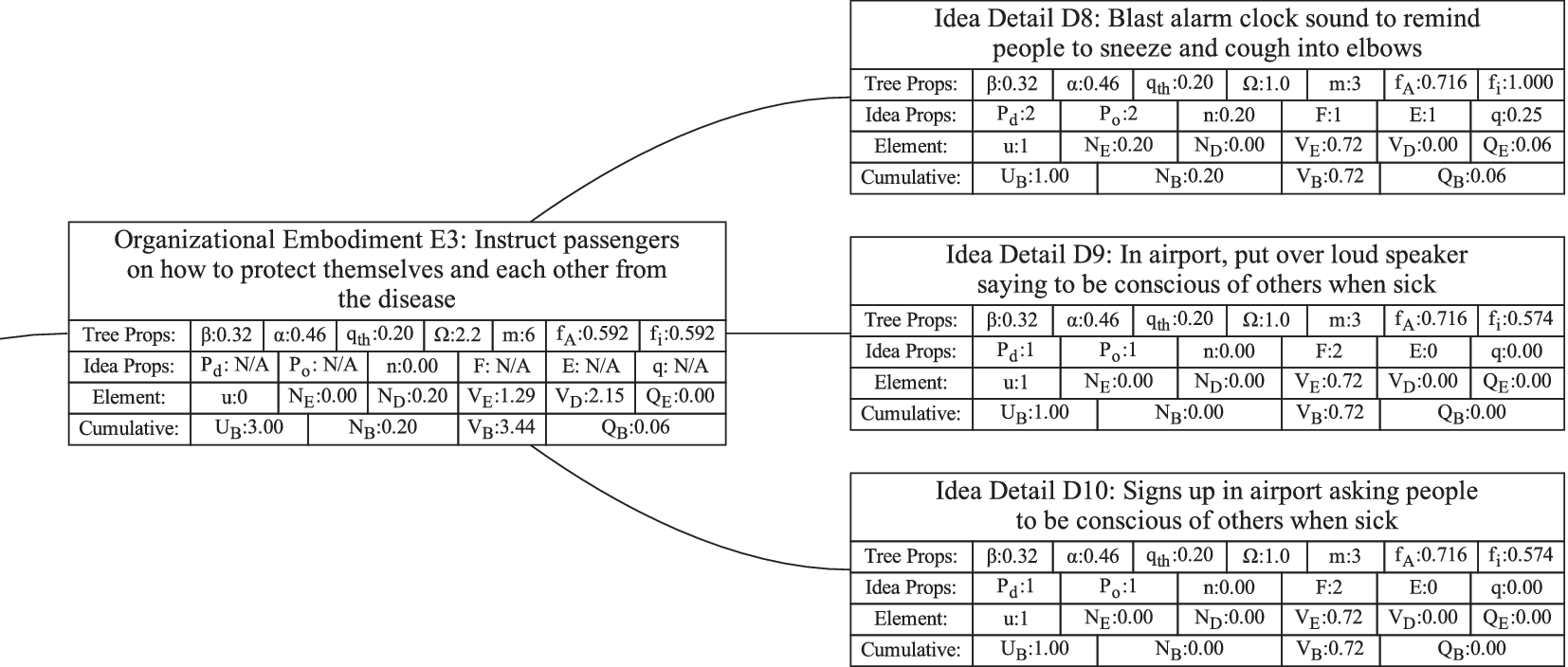
Subtree D: Three embodiments and two details of the diagnostic tree.
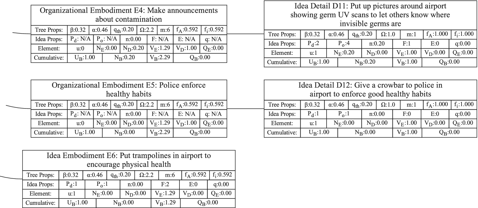
Subtree E: One objective and one principle of the diagnostic tree.
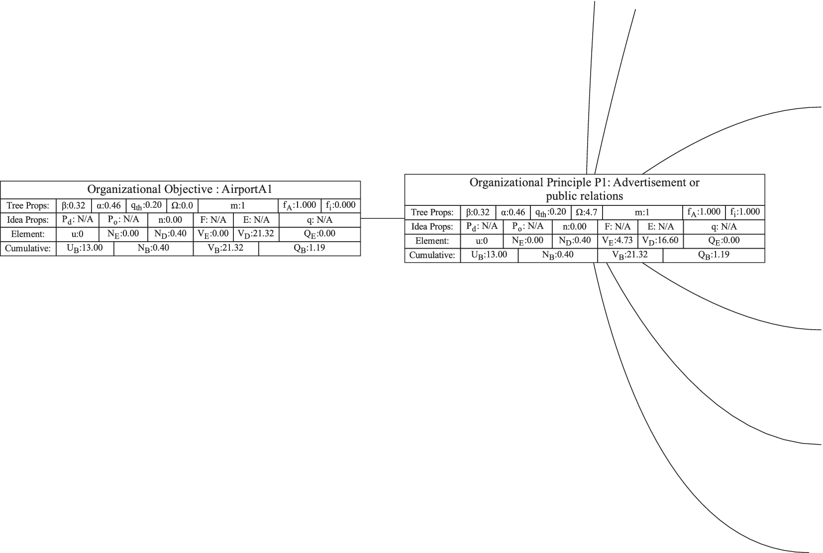


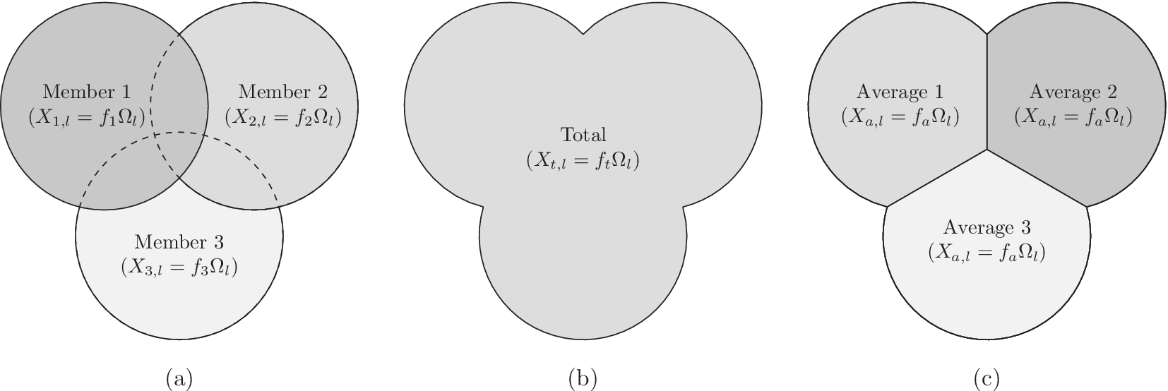


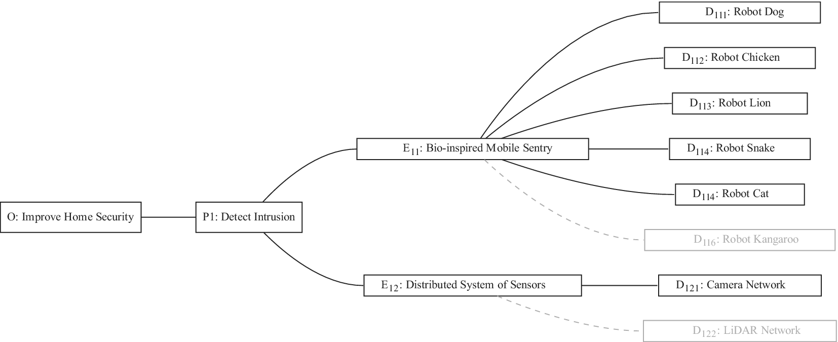


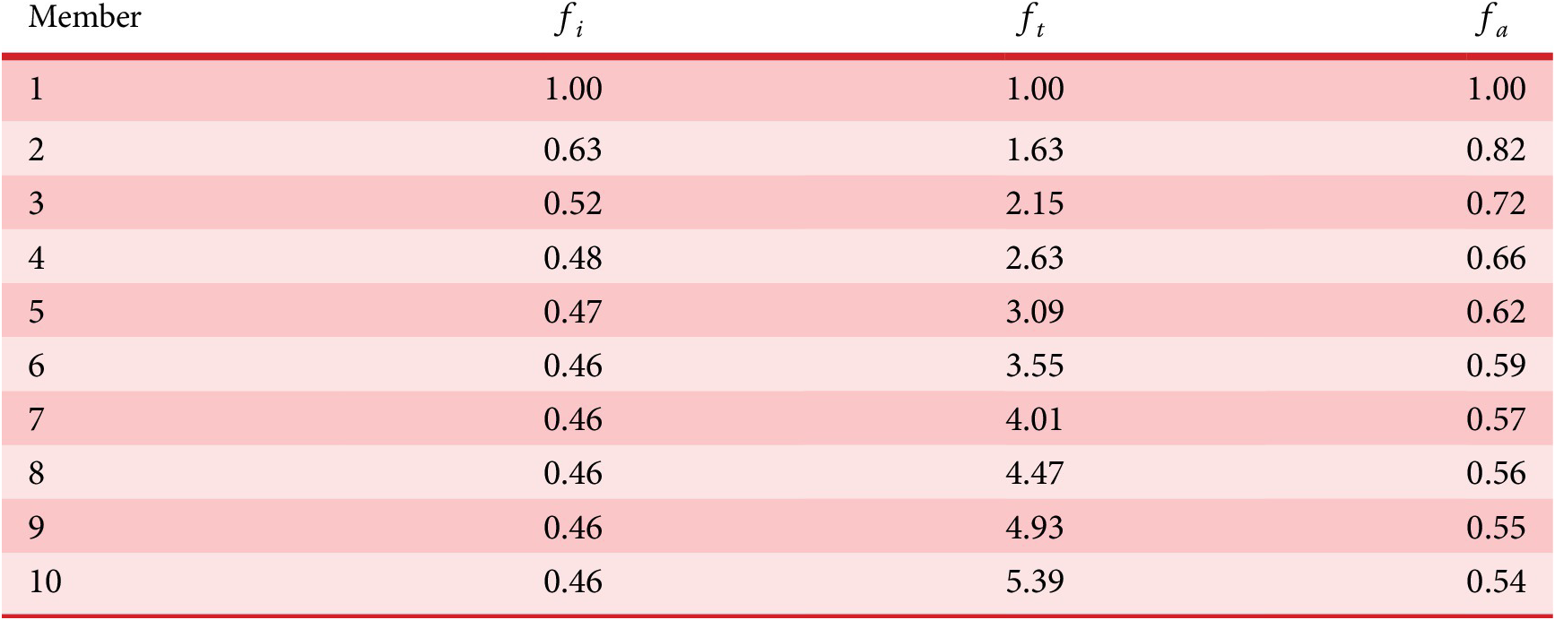


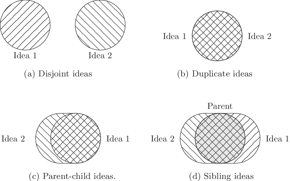


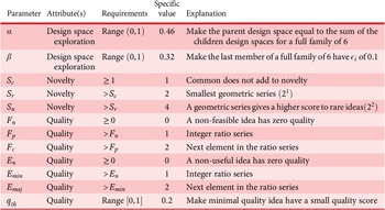
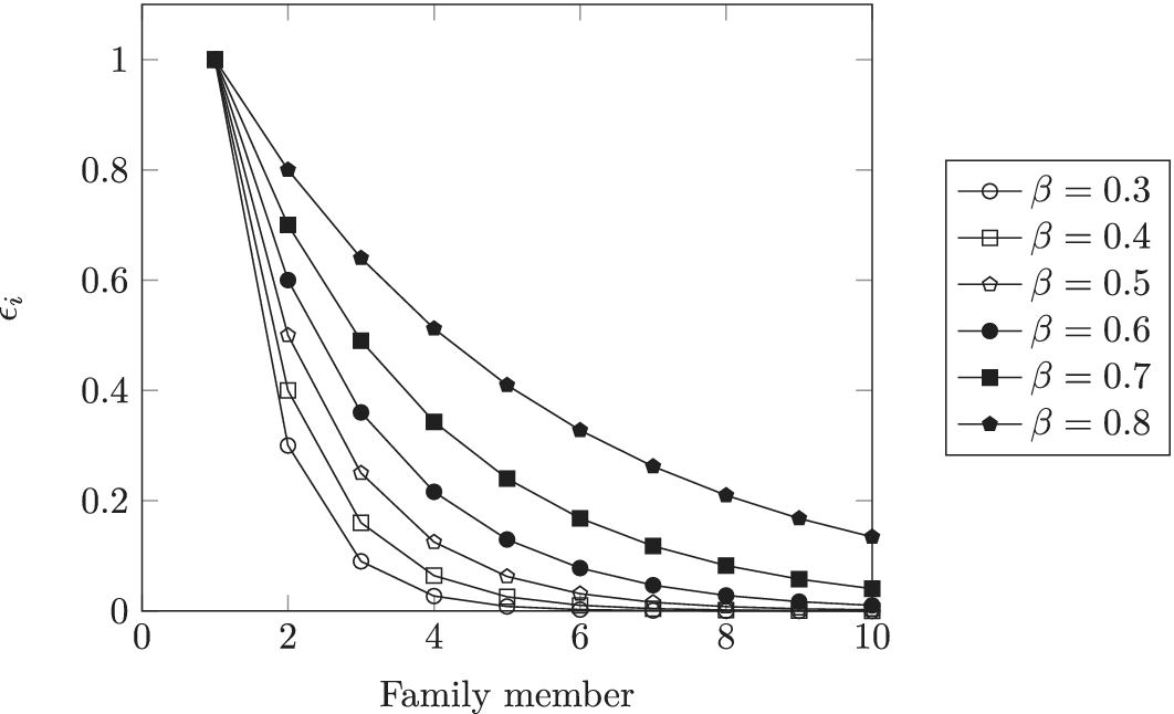


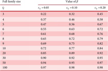


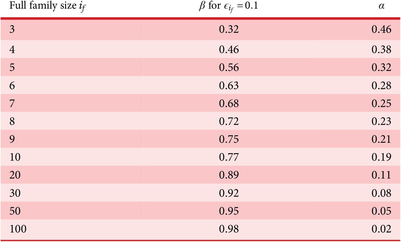


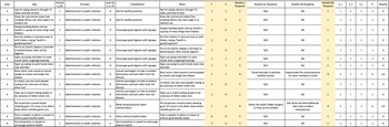
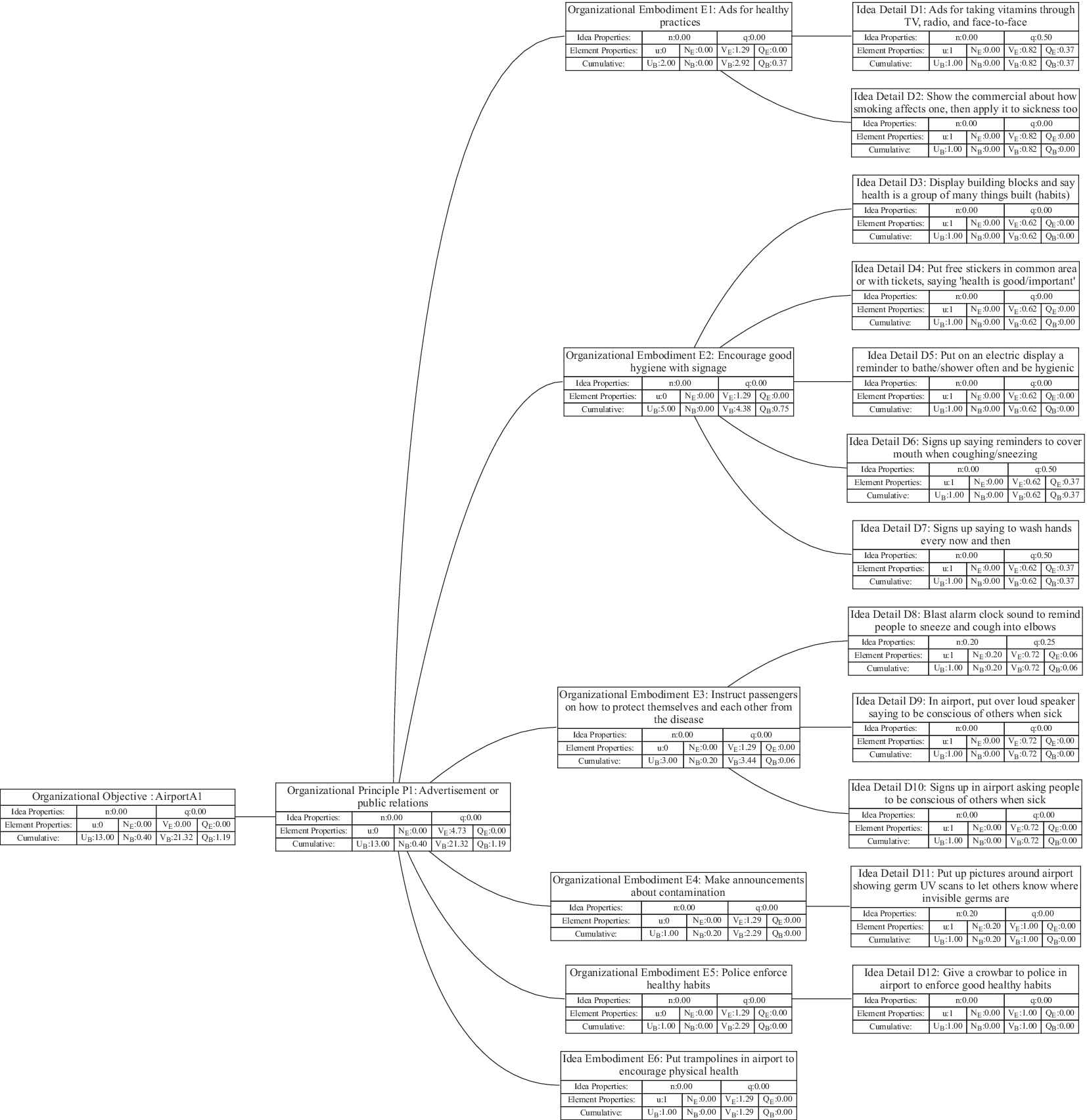

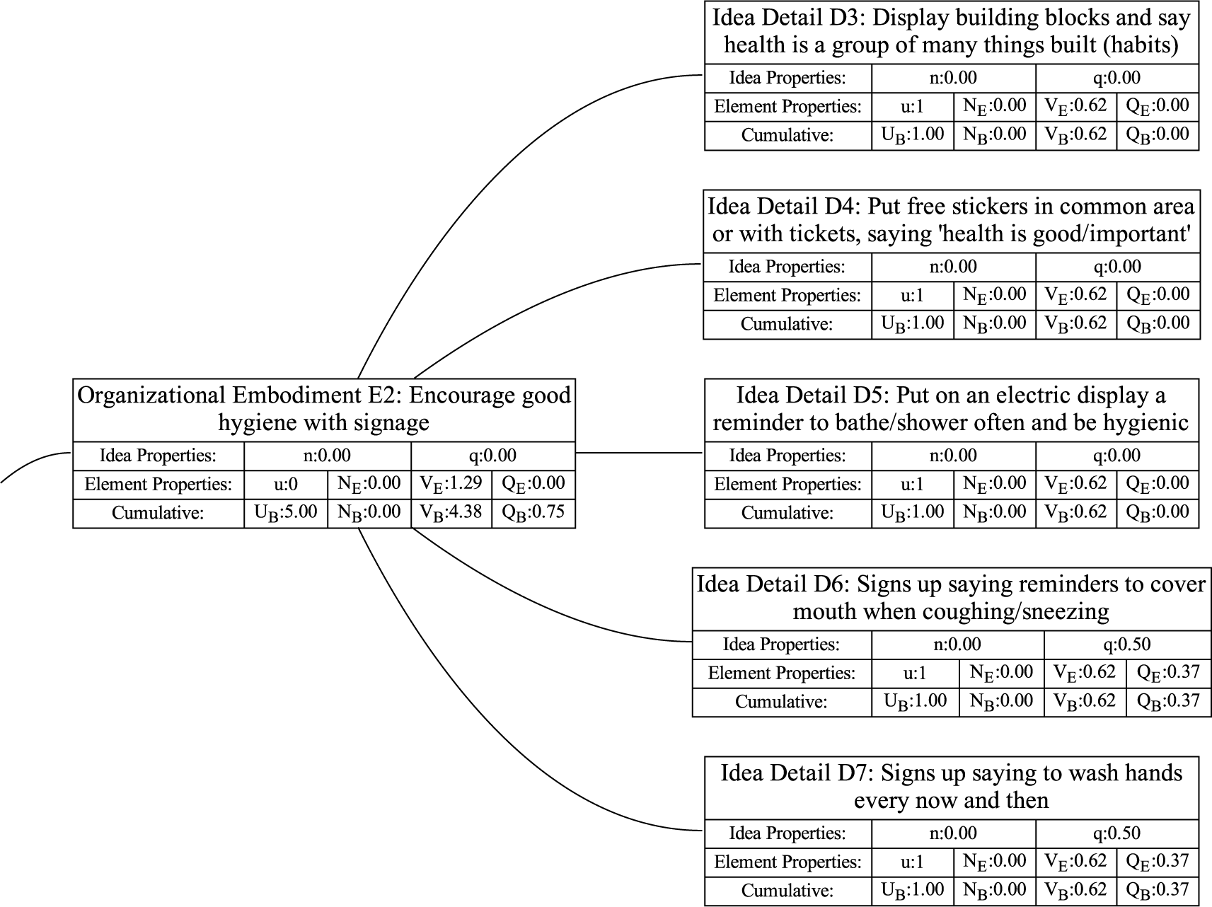

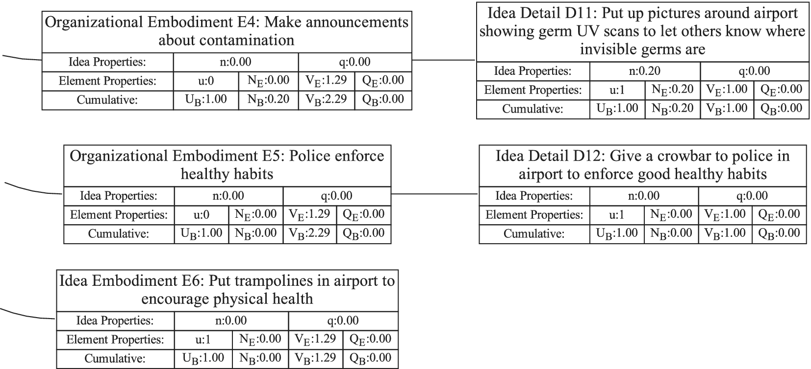


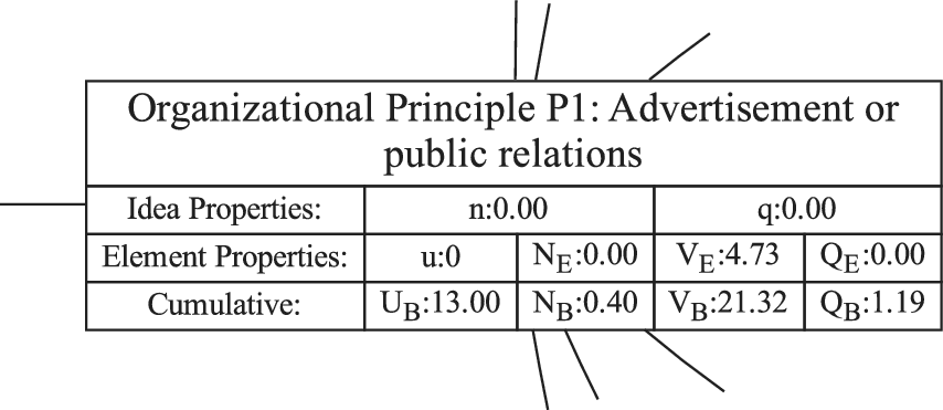


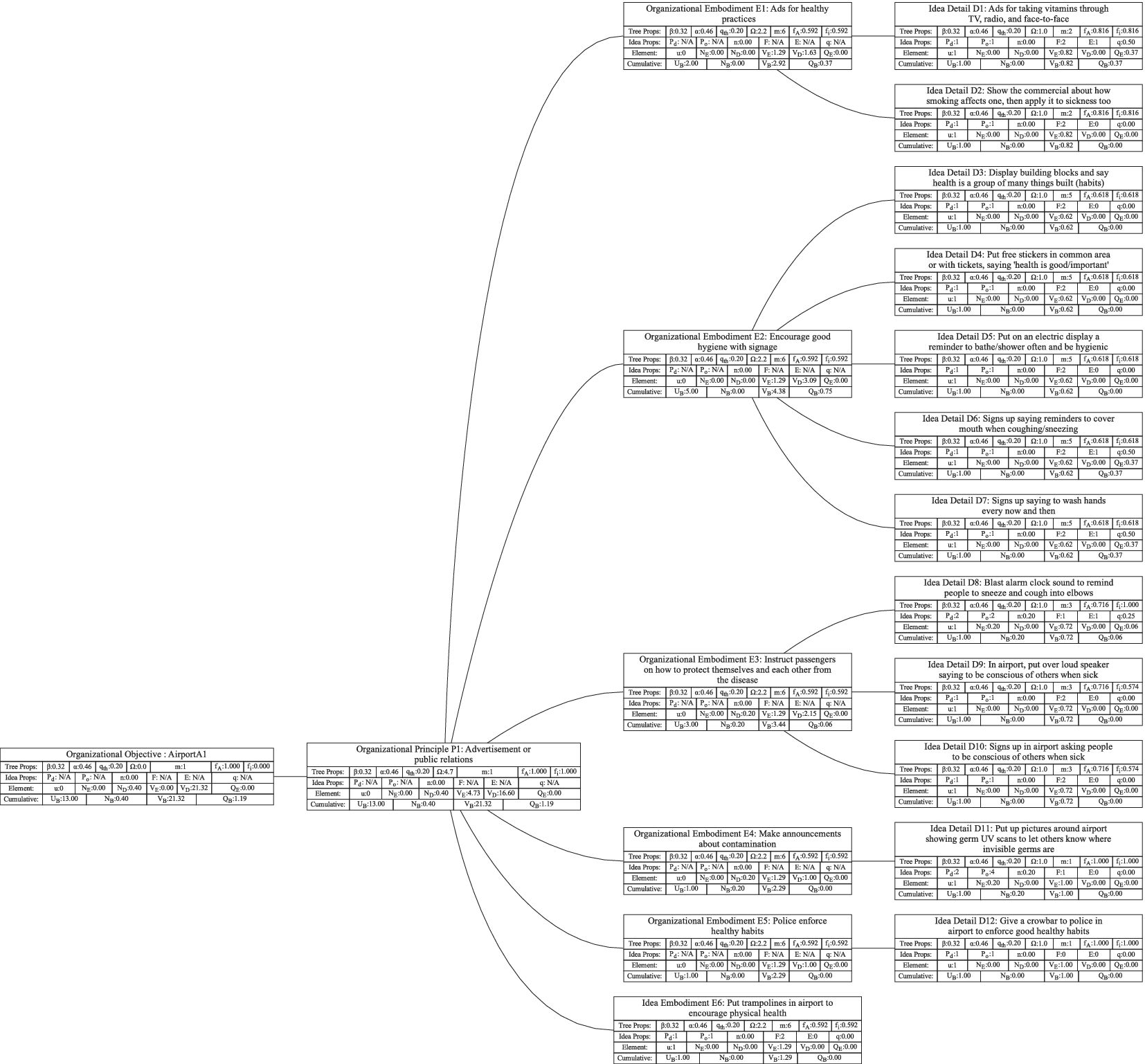

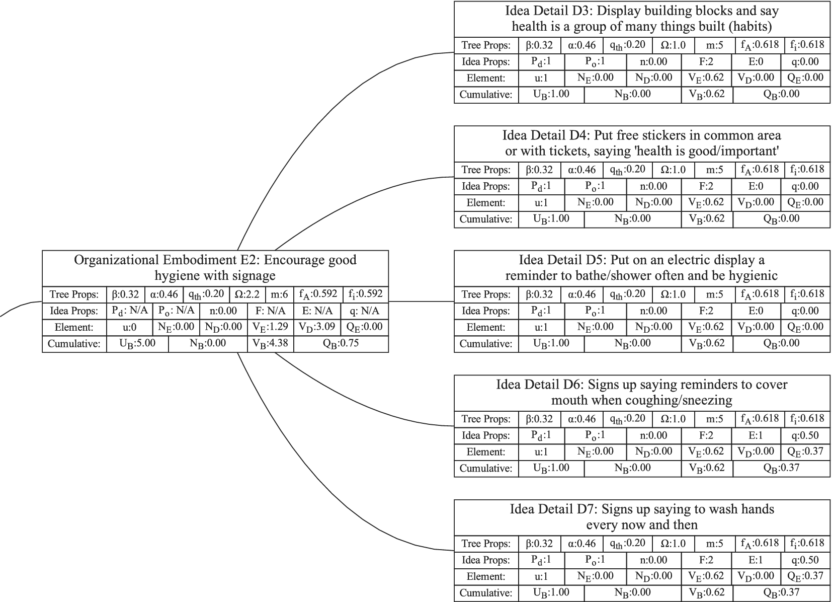


 Open access