


1. Introduction
Over their long evolutionary history, insects, birds, fish and many other organisms have evolved fast, efficient and agile locomotor abilities that are largely achieved through flapping wings or fins with diverse morphologies and oscillatory kinematics (Wu Reference Wu2011). The planform geometry of wings and fins can be described by several metrics, among which the aspect ratio ( ${\textit{AR}}$
) is a key parameter that measures how slender the platform is relative to its chordwise dimension and determines the propulsive performance (Sambilay Reference Sambilay1990; Combes & Daniel Reference Combes and Daniel2001; Usherwood & Ellington Reference Usherwood and Ellington2002; Walker & Westneat Reference Walker and Westneat2002; Kruyt et al. Reference Kruyt, van Heijst, Altshuler and Lentink2015). Interactions between high-
${\textit{AR}}$
) is a key parameter that measures how slender the platform is relative to its chordwise dimension and determines the propulsive performance (Sambilay Reference Sambilay1990; Combes & Daniel Reference Combes and Daniel2001; Usherwood & Ellington Reference Usherwood and Ellington2002; Walker & Westneat Reference Walker and Westneat2002; Kruyt et al. Reference Kruyt, van Heijst, Altshuler and Lentink2015). Interactions between high- ${\textit{AR}}$
flapping panels or foils in a tip-to-tip configuration characterised by the tips of the panels remaining closely aligned throughout the stroke cycle have been studied extensively due to interest in the hovering or forward flight dynamics of four-winged insects (Norberg Reference Norberg, Wu, Brokaw and Brennen1975; Sun & Lan Reference Sun and Lan2004; Wang & Sun Reference Wang and Sun2005; Wang & Russell Reference Wang and Russell2007; Hu & Deng Reference Hu and Deng2014; Bluman & Kang Reference Bluman and Kang2017; Liu et al. Reference Liu, Hefler, Fu, Shyy and Qiu2021). However, flow interactions between low-
${\textit{AR}}$
flapping panels or foils in a tip-to-tip configuration characterised by the tips of the panels remaining closely aligned throughout the stroke cycle have been studied extensively due to interest in the hovering or forward flight dynamics of four-winged insects (Norberg Reference Norberg, Wu, Brokaw and Brennen1975; Sun & Lan Reference Sun and Lan2004; Wang & Sun Reference Wang and Sun2005; Wang & Russell Reference Wang and Russell2007; Hu & Deng Reference Hu and Deng2014; Bluman & Kang Reference Bluman and Kang2017; Liu et al. Reference Liu, Hefler, Fu, Shyy and Qiu2021). However, flow interactions between low- ${\textit{AR}}$
panels in the tip-to-tip formation, such as vertically arranged fish tails shown in figure 1, have received limited attention.
${\textit{AR}}$
panels in the tip-to-tip formation, such as vertically arranged fish tails shown in figure 1, have received limited attention.
(a,b) Video frames from high-speed video of three giant danio swimming within a small school to show a vertical formation with the fish caudal fins in a tip-to-tip configuration at this time instant. Frames shown in (a) and (b) are from synchronised high-speed video recordings of the side and bottom views of the fish swimming against an imposed current. Vertical formations are one of several observed configurations of fish in schools (Ko et al. Reference Ko, Girma, Zhang, Pan, Lauder and Nagpal2025). (c,d) Three-dimensional body models of giant danio are arranged in the same configuration. Blue and orange dots in (a) and (b) identify the two individuals swimming in a vertical tip-to-tip configuration. Also see supplementary movies 1–3 available at https://doi.org/10.1017/jfm.2026.11175.

Dense fish schools exhibit a striking diversity of three-dimensional (3D) subformations. Field studies of wild fish aggregations involving large numbers of individuals suggest that, as self-organising dynamical systems, fish schools display highly dynamic and complex 3D internal structures, with both school height and density increasing with group size (Paramo et al. Reference Paramo, Bertrand, Villalobos and Gerlotto2007; Holland et al. Reference Holland, Becker, Smith, Everett and Suthers2021). Laboratory experiments on small fish species, such as zebrafish and Pacific blue-eyes, using 3D video tracking of medium-sized schools (approximately 10–20 individuals) confirm that fish frequently form compact vertical arrangements (Wang et al. Reference Wang, Zhao, Liu, Qian, Liu and Chen2017; Romenskyy et al. Reference Romenskyy, Herbert-Read, Ioannou, Szorkovszky, Ward and Sumpter2020). Long-term 3D tracking of six-fish giant danio (Devario aequipinnatus) schools swimming continuously for 10 hours further reveals that fish pairs are vertically aligned for approximately 79 % of the time (Ko et al. Reference Ko, Girma, Zhang, Pan, Lauder and Nagpal2025). In our recent experiments, schools of three to five giant danio (mean length 7 cm) were filmed in a recirculating flume at 2–6 body lengths per second using synchronised high-speed cameras (Photron mini-AX50) at 250 Hz. The recordings reveal frequent episodes in which two fish occupy vertically adjacent positions, with their caudal fins aligned tip-to-tip (figure 1 and supplementary movies 1–3).
In a two-dimensional (2D) plane, in-line, side-by-side and staggered configurations are basic arrangements that have been widely investigated to elucidate the hydrodynamic mechanisms underlying their performance advantages. These mechanisms can be broadly classified into wake–body, body–body and wake–wake interactions, through which swimmers can enhance thrust, reduce drag and lower power consumption. For example, in in-line and staggered formations, a following swimmer can harness energy from the leader’s vortex wake by adjusting its spatial position or kinematics, such as flapping phase and frequency, to achieve constructive wake–body synchronisation (Maertens, Gao & Triantafyllou Reference Maertens, Gao and Triantafyllou2017; Park & Sung Reference Park and Sung2018; Li et al. Reference Li, Nagy, Graving, Bak-Coleman, Xie and Couzin2020; Thandiackal & Lauder Reference Thandiackal and Lauder2023; Ormonde et al. Reference Ormonde, Kurt, Mivehchi and Moored2024). In side-by-side formations, swimmers can improve propulsive efficiency and enhance thrust production by tuning their phase difference and transverse spacing, with performance variations shown to correlate with the nature of wake interactions (Dewey et al. Reference Dewey, Quinn, Boschitsch and Smits2014; Huera-Huarte Reference Huera-Huarte2018; Gungor, Khalid & Hemmati Reference Gungor, Khalid and Hemmati2022). Moreover, body–body interactions have been implicated in hydrodynamic performance enhancement for both side-by-side and closely spaced staggered formations (Ormonde et al. Reference Ormonde, Kurt, Mivehchi and Moored2024; Rhodes & van Rees Reference Rhodes and van Rees2024). However, as a conspicuous 3D alternative, the vertical, tip-to-tip alignment of adjacent tails that emerges when fish stack above one another in dense schools has received far less attention.
The aspect ratio of propulsors exerts a first-order influence on the locomotor strategies of both flyers and swimmers, as well as on the attendant vortex dynamics. Statistical surveys place the mean ${\textit{AR}}$
of four-winged insects above 3.5 (Nan et al. Reference Nan, Peng, Chen, Feng and McGlinchey2018); dragonflies, for example, possess wings with
${\textit{AR}}$
of four-winged insects above 3.5 (Nan et al. Reference Nan, Peng, Chen, Feng and McGlinchey2018); dragonflies, for example, possess wings with ${\textit{AR}}\approx 5$
(Norberg Reference Norberg, Wu, Brokaw and Brennen1975). By contrast, many fish employ fins whose
${\textit{AR}}\approx 5$
(Norberg Reference Norberg, Wu, Brokaw and Brennen1975). By contrast, many fish employ fins whose ${\textit{AR}}$
lies well below two (Weihs Reference Weihs1989; Sambilay Reference Sambilay1990). Lake trout (Salvelinus namaycush) exhibit caudal fins with
${\textit{AR}}$
lies well below two (Weihs Reference Weihs1989; Sambilay Reference Sambilay1990). Lake trout (Salvelinus namaycush) exhibit caudal fins with ${\textit{AR}}\approx 1$
, and sand gobies attain values as low as 0.6 (Sambilay Reference Sambilay1990). The
${\textit{AR}}\approx 1$
, and sand gobies attain values as low as 0.6 (Sambilay Reference Sambilay1990). The ${\textit{AR}}$
of pectoral fins of some Labrid fish species is approximately 1.5 (Wainwright, Bellwood & Westneat Reference Wainwright, Bellwood and Westneat2002; Walker & Westneat Reference Walker and Westneat2002), and brook trout (Salvelinus fontinalis) dorsal fins have an
${\textit{AR}}$
of pectoral fins of some Labrid fish species is approximately 1.5 (Wainwright, Bellwood & Westneat Reference Wainwright, Bellwood and Westneat2002; Walker & Westneat Reference Walker and Westneat2002), and brook trout (Salvelinus fontinalis) dorsal fins have an ${\textit{AR}}$
of approximately 1.8 (Standen & Lauder Reference Standen and Lauder2007). Throughout this paper,
${\textit{AR}}$
of approximately 1.8 (Standen & Lauder Reference Standen and Lauder2007). Throughout this paper, ${\textit{AR}}$
is defined as
${\textit{AR}}$
is defined as $b^{2}/S$
, where
$b^{2}/S$
, where $b$
is the span and
$b$
is the span and $S$
is the planform area. A high
$S$
is the planform area. A high ${\textit{AR}}$
permits insects and birds to generate large lift with reduced lift-induced drag (Alexander Reference Alexander2002); a low
${\textit{AR}}$
permits insects and birds to generate large lift with reduced lift-induced drag (Alexander Reference Alexander2002); a low ${\textit{AR}}$
, in turn, mitigates vortex-induced drag for fish (Yeh & Alexeev Reference Yeh and Alexeev2016) and can enhance thrust production (Green & Smits Reference Green and Smits2008), acceleration (Webb Reference Webb1994; Domenici & Blake Reference Domenici and Blake1997) and manoeuvrability (Flammang & Lauder Reference Flammang and Lauder2009), while lowering bending moments that predispose fin damage (Dong, Mittal & Najjar Reference Dong, Mittal and Najjar2006).
${\textit{AR}}$
, in turn, mitigates vortex-induced drag for fish (Yeh & Alexeev Reference Yeh and Alexeev2016) and can enhance thrust production (Green & Smits Reference Green and Smits2008), acceleration (Webb Reference Webb1994; Domenici & Blake Reference Domenici and Blake1997) and manoeuvrability (Flammang & Lauder Reference Flammang and Lauder2009), while lowering bending moments that predispose fin damage (Dong, Mittal & Najjar Reference Dong, Mittal and Najjar2006).
Aspect ratio also determines the wake topology of flapping foils. At high ${\textit{AR}}$
, two spanwise vortices with opposite signs are shed from the trailing edge of an oscillating foil during each flapping cycle, forming a
${\textit{AR}}$
, two spanwise vortices with opposite signs are shed from the trailing edge of an oscillating foil during each flapping cycle, forming a $2S$
wake that transitions into a reverse von Kármán vortex street when the Strouhal number is within the optimal range (
$2S$
wake that transitions into a reverse von Kármán vortex street when the Strouhal number is within the optimal range ( $0.25\leq St\leq 0.35$
) (Triantafyllou, Triantafyllou & Grosenbaugh Reference Triantafyllou, Triantafyllou and Grosenbaugh1993). As
$0.25\leq St\leq 0.35$
) (Triantafyllou, Triantafyllou & Grosenbaugh Reference Triantafyllou, Triantafyllou and Grosenbaugh1993). As ${\textit{AR}}$
decreases, streamwise vortices generated at the top and bottom panel tips are enhanced and gradually connected to the spanwise vortices (Green & Smits Reference Green and Smits2008; De & Sarkar Reference De and Sarkar2024). At low
${\textit{AR}}$
decreases, streamwise vortices generated at the top and bottom panel tips are enhanced and gradually connected to the spanwise vortices (Green & Smits Reference Green and Smits2008; De & Sarkar Reference De and Sarkar2024). At low ${\textit{AR}}$
, streamwise vortices rival the spanwise vortices in strength and dominate the evolution of the vortex wake (Buchholz & Smits Reference Buchholz and Smits2006). Numerous experiments and simulations have shown that low-
${\textit{AR}}$
, streamwise vortices rival the spanwise vortices in strength and dominate the evolution of the vortex wake (Buchholz & Smits Reference Buchholz and Smits2006). Numerous experiments and simulations have shown that low- ${\textit{AR}}$
flapping foils generate vortex wake characterised by interconnected vortex loops, which subsequently evolve and disconnect into distinct vortex rings downstream (Buchholz & Smits Reference Buchholz and Smits2006, Reference Buchholz and Smits2008; Green, Rowley & Smits Reference Green, Rowley and Smits2011). Dong et al. (Reference Dong, Mittal and Najjar2006) also observed that the vortex rings convect downstream at an angle to the streamwise direction, leading to the formation of twin oblique jets. The evolution of low-
${\textit{AR}}$
flapping foils generate vortex wake characterised by interconnected vortex loops, which subsequently evolve and disconnect into distinct vortex rings downstream (Buchholz & Smits Reference Buchholz and Smits2006, Reference Buchholz and Smits2008; Green, Rowley & Smits Reference Green, Rowley and Smits2011). Dong et al. (Reference Dong, Mittal and Najjar2006) also observed that the vortex rings convect downstream at an angle to the streamwise direction, leading to the formation of twin oblique jets. The evolution of low- ${\textit{AR}}$
panel wake pattern was confirmed by digital particle image velocimetry (DPIV) measurement in live fish swimming, such as a series of linked elliptical vortex rings generated by caudal fin (
${\textit{AR}}$
panel wake pattern was confirmed by digital particle image velocimetry (DPIV) measurement in live fish swimming, such as a series of linked elliptical vortex rings generated by caudal fin ( ${\textit{AR}}\approx 0.6$
) of chub mackerel (Scomber japonicus) (Nauen & Lauder Reference Nauen and Lauder2002) and a train of separated vortex rings shed by the pectoral fin (
${\textit{AR}}\approx 0.6$
) of chub mackerel (Scomber japonicus) (Nauen & Lauder Reference Nauen and Lauder2002) and a train of separated vortex rings shed by the pectoral fin ( ${\textit{AR}}\approx 1.8$
) of bluegill sunfish (Drucker & Lauder Reference Drucker and Lauder1999).
${\textit{AR}}\approx 1.8$
) of bluegill sunfish (Drucker & Lauder Reference Drucker and Lauder1999).
Tip-to-tip interactions between high- ${\textit{AR}}$
wings are well documented in four-winged insects. By adjusting the streamwise offset and phase difference between the fore- and hind-wings, these flyers manipulate wing–wake and vortex interactions to boost lift (Lehmann Reference Lehmann2009; Xie & Huang Reference Xie and Huang2015) or minimise energetic cost (Wang & Russell Reference Wang and Russell2007). Equivalent studies for low-
${\textit{AR}}$
wings are well documented in four-winged insects. By adjusting the streamwise offset and phase difference between the fore- and hind-wings, these flyers manipulate wing–wake and vortex interactions to boost lift (Lehmann Reference Lehmann2009; Xie & Huang Reference Xie and Huang2015) or minimise energetic cost (Wang & Russell Reference Wang and Russell2007). Equivalent studies for low- ${\textit{AR}}$
appendages are scarce, partly because anatomical examples are rare. Collective fish behaviour, however, provides natural instances of vertically stacked, low-
${\textit{AR}}$
appendages are scarce, partly because anatomical examples are rare. Collective fish behaviour, however, provides natural instances of vertically stacked, low- ${\textit{AR}}$
fins. A recent numerical study considered vertically aligned tuna-like bodies (Li et al. Reference Li, Gu, Su and Yao2021), but, owing to their high-
${\textit{AR}}$
fins. A recent numerical study considered vertically aligned tuna-like bodies (Li et al. Reference Li, Gu, Su and Yao2021), but, owing to their high- ${\textit{AR}}$
lunate fins (>3), trunk–fin coupling dominated, and tail–tail coupling was weak. Species such as giant danio and trout, whose caudal fins possess low
${\textit{AR}}$
lunate fins (>3), trunk–fin coupling dominated, and tail–tail coupling was weak. Species such as giant danio and trout, whose caudal fins possess low ${\textit{AR}}$
, generate span-expanded vortex wakes, ideal for near-field fin–fin interaction (Pan et al. Reference Pan, Zhang, Kelly and Dong2024; Menzer et al. Reference Menzer, Pan, Lauder and Dong2025); yet no study has quantified the hydrodynamic consequences of aligning such tails tip-to-tip.
${\textit{AR}}$
, generate span-expanded vortex wakes, ideal for near-field fin–fin interaction (Pan et al. Reference Pan, Zhang, Kelly and Dong2024; Menzer et al. Reference Menzer, Pan, Lauder and Dong2025); yet no study has quantified the hydrodynamic consequences of aligning such tails tip-to-tip.
The present study explores hydrodynamic interactions between two identical trapezoidal panels with an aspect ratio of ${\textit{AR}}=1.2$
arranged in a tip-to-tip formation. Section 2 provides a detailed description of the panel geometry, kinematics and the tip-to-tip configuration, together with the numerical and experimental methods. Section 3 presents immersed-boundary simulations at
${\textit{AR}}=1.2$
arranged in a tip-to-tip formation. Section 2 provides a detailed description of the panel geometry, kinematics and the tip-to-tip configuration, together with the numerical and experimental methods. Section 3 presents immersed-boundary simulations at $Re=600$
, which sweep through vertical gap and phase offset values to map the resulting forces and efficiencies relative to an isolated panel. The accompanying flow fields are analysed to reveal the underlying flow physics. In addition, we generalise the results from two-panel systems to multi-panel configurations, extend the simulations to
$Re=600$
, which sweep through vertical gap and phase offset values to map the resulting forces and efficiencies relative to an isolated panel. The accompanying flow fields are analysed to reveal the underlying flow physics. In addition, we generalise the results from two-panel systems to multi-panel configurations, extend the simulations to $Re=2000$
–
$Re=2000$
– $10\,000$
and perform water-channel experiments at
$10\,000$
and perform water-channel experiments at $Re=10\,000$
–
$Re=10\,000$
– $30\,000$
. Collectively, these data delineate how tip-to-tip coupling reshapes the wake of low-aspect-ratio fins and how schools may exploit this configuration to modulate thrust, lift and energetic cost.
$30\,000$
. Collectively, these data delineate how tip-to-tip coupling reshapes the wake of low-aspect-ratio fins and how schools may exploit this configuration to modulate thrust, lift and energetic cost.
2. Materials and methods
2.1. Panel model, kinematics and tip-to-tip configuration
The geometry of a trapezoidal panel was modelled based on a general low- ${\textit{AR}}$
caudal fin shape found in various fish species where aspect ratios can approach 1.0 (Helfman, Collette & Facey Reference Helfman, Collette and Facey1997). The relevant parameters are shown in figure 2(a), where
${\textit{AR}}$
caudal fin shape found in various fish species where aspect ratios can approach 1.0 (Helfman, Collette & Facey Reference Helfman, Collette and Facey1997). The relevant parameters are shown in figure 2(a), where $a$
,
$a$
, $b$
,
$b$
, $c$
represent the spans at the edges and the chord length of the panel, respectively. The trapezoidal panel used in the current study has a low
$c$
represent the spans at the edges and the chord length of the panel, respectively. The trapezoidal panel used in the current study has a low ${\textit{AR}}$
of 1.2 defined based on the longer span, close to the trout caudal fin (
${\textit{AR}}$
of 1.2 defined based on the longer span, close to the trout caudal fin ( ${\textit{AR}}=1.3$
) used in a previous study (Pan et al. Reference Pan, Zhang, Kelly and Dong2024). The panel is pitched about the leading edge and simultaneously undergoes a harmonic translational motion, i.e. a heaving motion, along the y-axis (see figure 2
b). The following equations describe the motions:
${\textit{AR}}=1.3$
) used in a previous study (Pan et al. Reference Pan, Zhang, Kelly and Dong2024). The panel is pitched about the leading edge and simultaneously undergoes a harmonic translational motion, i.e. a heaving motion, along the y-axis (see figure 2
b). The following equations describe the motions:
 \begin{align} \theta \left(t\right) &=\theta _{0}\sin\left(2\pi ft+\varphi \right), \end{align}
 \begin{align} y\left(t\right) &=\frac{y_{0}}{2}\cos\left(2\pi ft+\varphi \right), \end{align}
(a) Geometry of trapezoidal panel model, (b) top view of the pitching–heaving motion with an incoming flow and (c) schematic of two panels in a tip-to-tip configuration separated by distance $H$
.
$H$
. $U_{\infty}$
denotes the incoming flow velocity.
$U_{\infty}$
denotes the incoming flow velocity.

where $\theta _{0}=15^{\circ}$
denotes the amplitude of the pitching motion,
$\theta _{0}=15^{\circ}$
denotes the amplitude of the pitching motion, $y_{0}=0.4c$
is the peak-to-peak amplitude of the heaving motion, and
$y_{0}=0.4c$
is the peak-to-peak amplitude of the heaving motion, and $t$
is time. In this study, for simplicity, the pitching and heaving motions share the same frequency and phase. Accordingly,
$t$
is time. In this study, for simplicity, the pitching and heaving motions share the same frequency and phase. Accordingly, $f$
and
$f$
and $\varphi$
represent the driving frequency and phase, respectively, of the coupled motion of a panel. When two panels are vertically arranged, as shown in figure 2(c),
$\varphi$
represent the driving frequency and phase, respectively, of the coupled motion of a panel. When two panels are vertically arranged, as shown in figure 2(c), $\varphi _{1}$
and
$\varphi _{1}$
and $\varphi _{2}$
denote the phase of panel 1 and panel 2, respectively, and
$\varphi _{2}$
denote the phase of panel 1 and panel 2, respectively, and $H$
represents the tip-to-tip distance between the panels.
$H$
represents the tip-to-tip distance between the panels.
2.2. Numerical methods
The governing equations of the flow problems solved are the 3D incompressible viscous Navier–Stokes equations, written in the indicial form as
 \begin{equation}\frac{\partial u_{i}}{\partial x_{i}}=0; \quad \frac{\partial u_{i}}{\partial t}+\frac{\partial (u_{i}u_{j})}{\partial x_{j}}=-\frac{1}{\rho }\frac{\partial p}{\partial x_{i}}+\nu \frac{\partial ^{2}u_{i}}{\partial x_{j}\partial x_{j}},\end{equation}
where $i,j=1,2$
or 3, and
$i,j=1,2$
or 3, and $u_{i}$
are the velocity components in the x-, y- and z-directions,
$u_{i}$
are the velocity components in the x-, y- and z-directions, $p$
is the pressure,
$p$
is the pressure, $\rho$
is the fluid density, and
$\rho$
is the fluid density, and $\nu$
is the fluid kinematic viscosity.
$\nu$
is the fluid kinematic viscosity.
Incompressible flow was computed using an immersed-boundary method (IBM) based on finite-difference schemes (Mittal et al. Reference Mittal, Dong, Bozkurttas, Najjar, Vargas and Von Loebbecke2008). The governing equations were spatially discretised using a collocated, cell-centred arrangement of the primitive variables, $u_{i}$
and
$u_{i}$
and $p$
, and were temporally integrated via a fractional step approach. To handle the convection terms, a second-order Adams–Bashforth scheme was applied, while the viscous terms were treated implicitly using the Crank–Nicolson method to alleviate the viscous stability constraint. The simulations were constructed on non-conformal Cartesian grids, with boundary conditions accurately enforced on the immersed surfaces using a multi-dimensional ghost-cell strategy. We also employed a tree-topological local mesh refinement (TLMR) method on the Cartesian grids combined with parallel computing techniques to improve computational efficiency (Zhang et al. Reference Zhang, Pan, Wang, Di Santo, Lauder and Dong2023) and a narrow-band level-set method for highly efficient moving boundary reconstruction (Pan, Dong & Zhang Reference Pan, Dong and Zhang2021). This numerical framework has been successfully applied to simulate oscillating propulsions (Pan, Wang & Dong Reference Pan, Wang and Dong2019; Han et al. Reference Han, Pan, Liu and Dong2022).
$p$
, and were temporally integrated via a fractional step approach. To handle the convection terms, a second-order Adams–Bashforth scheme was applied, while the viscous terms were treated implicitly using the Crank–Nicolson method to alleviate the viscous stability constraint. The simulations were constructed on non-conformal Cartesian grids, with boundary conditions accurately enforced on the immersed surfaces using a multi-dimensional ghost-cell strategy. We also employed a tree-topological local mesh refinement (TLMR) method on the Cartesian grids combined with parallel computing techniques to improve computational efficiency (Zhang et al. Reference Zhang, Pan, Wang, Di Santo, Lauder and Dong2023) and a narrow-band level-set method for highly efficient moving boundary reconstruction (Pan, Dong & Zhang Reference Pan, Dong and Zhang2021). This numerical framework has been successfully applied to simulate oscillating propulsions (Pan, Wang & Dong Reference Pan, Wang and Dong2019; Han et al. Reference Han, Pan, Liu and Dong2022).
The Cartesian grid with local refinement blocks and the boundary conditions for the simulations of the pitching–heaving panels are shown in figure 3. The size of the computation domain was $16c\times 14c\times 14c$
, with approximately 2.1 million (
$16c\times 14c\times 14c$
, with approximately 2.1 million ( $145\times 113\times 129$
) total grid points on the base layer. The computational domain size was determined based on numerous previously published studies. Detailed domain-size sensitivity analyses were conducted in earlier works on 3D fish-like swimming and oscillating foils (Han et al. Reference Han, Pan, Liu and Dong2022; Pan et al. Reference Pan, Zhang, Kelly and Dong2024), confirming that the present domain size ensures accurate wake development without spurious boundary effects. To accurately resolve the flow near the panels, two layers of refined meshes, represented by the red and blue blocks in figure 3(a), were applied, yielding the finest grid resolution of
$145\times 113\times 129$
) total grid points on the base layer. The computational domain size was determined based on numerous previously published studies. Detailed domain-size sensitivity analyses were conducted in earlier works on 3D fish-like swimming and oscillating foils (Han et al. Reference Han, Pan, Liu and Dong2022; Pan et al. Reference Pan, Zhang, Kelly and Dong2024), confirming that the present domain size ensures accurate wake development without spurious boundary effects. To accurately resolve the flow near the panels, two layers of refined meshes, represented by the red and blue blocks in figure 3(a), were applied, yielding the finest grid resolution of ${\unicode{x0394}} _{\textit{min}}=0.011c$
near the panels. A uniform inflow velocity was prescribed at the left boundary. At the right boundary, an outflow condition with zero normal velocity gradients was applied, allowing vortices to convect smoothly out of the computational domain without reflections. Zero-gradient (Neumann) boundary conditions for velocity were imposed on the lateral boundaries. Pressure boundary conditions were the homogeneous Neumann boundary condition applied at all boundaries. In addition, a grid convergence study was conducted for the pitching–heaving panel simulations. Figure 3(b) displays the time histories of the thrust coefficient of panel 1 (identical to panel 2) in the paired configuration with the minimum spacing
${\unicode{x0394}} _{\textit{min}}=0.011c$
near the panels. A uniform inflow velocity was prescribed at the left boundary. At the right boundary, an outflow condition with zero normal velocity gradients was applied, allowing vortices to convect smoothly out of the computational domain without reflections. Zero-gradient (Neumann) boundary conditions for velocity were imposed on the lateral boundaries. Pressure boundary conditions were the homogeneous Neumann boundary condition applied at all boundaries. In addition, a grid convergence study was conducted for the pitching–heaving panel simulations. Figure 3(b) displays the time histories of the thrust coefficient of panel 1 (identical to panel 2) in the paired configuration with the minimum spacing $H=0.1c$
, computed using four mesh resolutions: coarse, medium, fine and dense meshes. The finest grid spacings of these meshes were
$H=0.1c$
, computed using four mesh resolutions: coarse, medium, fine and dense meshes. The finest grid spacings of these meshes were $0.045c$
,
$0.045c$
, $0.023c$
,
$0.023c$
, $0.011c$
and
$0.011c$
and $0.006c$
, respectively. The thrust coefficients exhibited progressive convergence as the grid is refined. The difference in mean thrust between the fine and dense meshes was approximately 2.1 %, indicating that the flow simulations performed on the mesh of
$0.006c$
, respectively. The thrust coefficients exhibited progressive convergence as the grid is refined. The difference in mean thrust between the fine and dense meshes was approximately 2.1 %, indicating that the flow simulations performed on the mesh of ${\unicode{x0394}} _{\textit{min}}=0.011c$
are sufficiently converged at
${\unicode{x0394}} _{\textit{min}}=0.011c$
are sufficiently converged at $Re=600$
, as further grid refinement leads to negligible changes in the computed flow quantities. This mesh resolution is consistent with those employed in previous studies that examined interactions between multiple tandem pitching panels at similar Reynolds numbers (Wang et al. Reference Wang, Wainwright, Lindengren, Lauder and Dong2020; Han et al. Reference Han, Pan, Liu and Dong2022). Moreover, for the simulations conducted at higher Reynolds numbers in this study, finer meshes were employed, and corresponding grid-independence tests were performed separately.
$Re=600$
, as further grid refinement leads to negligible changes in the computed flow quantities. This mesh resolution is consistent with those employed in previous studies that examined interactions between multiple tandem pitching panels at similar Reynolds numbers (Wang et al. Reference Wang, Wainwright, Lindengren, Lauder and Dong2020; Han et al. Reference Han, Pan, Liu and Dong2022). Moreover, for the simulations conducted at higher Reynolds numbers in this study, finer meshes were employed, and corresponding grid-independence tests were performed separately.
(a) Schematic of computational mesh and boundary conditions for the pitching–heaving trapezoidal panels in a tip-to-tip configuration. (b) Comparison of the instantaneous thrust coefficients of panel 1 (identical to panel 2) in a tip-to-tip pitching–heaving panel formation at $H=0.1c$
computed at the coarse (
$H=0.1c$
computed at the coarse ( ${\unicode{x0394}} _{\textit{min}}=0.045c$
), medium (
${\unicode{x0394}} _{\textit{min}}=0.045c$
), medium ( ${\unicode{x0394}} _{\textit{min}}=0.023c$
), fine (
${\unicode{x0394}} _{\textit{min}}=0.023c$
), fine ( ${\unicode{x0394}} _{\textit{min}}=0.011c$
) and dense (
${\unicode{x0394}} _{\textit{min}}=0.011c$
) and dense ( ${\unicode{x0394}} _{\textit{min}}=0.006c$
) meshes.
${\unicode{x0394}} _{\textit{min}}=0.006c$
) meshes. $C_T$
denotes the thrust coefficient.
$C_T$
denotes the thrust coefficient.

2.3. Experimental methods
We oscillated the panels in a closed-loop water channel with a test section of $0.38\,{\textrm{m}}\times 0.45\,{\textrm{m}}\times 1.52\,{\textrm{m}}$
(width × height × length) to cross-validate with simulation results and to extend the Reynolds-number range of the present study. A schematic of the experimental set-up is shown in figure 4. We tested a single panel as the baseline case and four sets of paired panels with
$0.38\,{\textrm{m}}\times 0.45\,{\textrm{m}}\times 1.52\,{\textrm{m}}$
(width × height × length) to cross-validate with simulation results and to extend the Reynolds-number range of the present study. A schematic of the experimental set-up is shown in figure 4. We tested a single panel as the baseline case and four sets of paired panels with $H$
varied from 0 to 0.1
$H$
varied from 0 to 0.1 $c$
, 0.25
$c$
, 0.25 $c$
and 0.5
$c$
and 0.5 $c$
to study the effect of vertical distance
$c$
to study the effect of vertical distance $H$
. In the experiments, each panel had a chord length of 0.0762 m and its trapezoidal geometry matched the model used in simulations. The paired panels were connected using a carbon fibre shaft, which was further attached to a six-axis force/torque sensor (ATI Mini40 IP65) for measuring hydrodynamic forces. To reduce the influence of the carbon fibre on measurements, a teardrop cross-section is used for the panels. The pitching–heaving motion of the panels was prescribed by two servo motors (Teknic CPM-MCPV-2341S-ELN, coupled with 5:1 gearbox, SureGear PGCN23-0525), with the panel kinematics matching those used in the simulations. The motions of panels 1 and 2 were in phase, measured using a rotary encoder (US Digital EM2-1-5000-I) and a linear encoder (US Digital EM2-0-2000-I). In each experimental trial, we prescribed 50 pitch–heave cycles, with 5 additional ramp-up cycles and 5 ramp-down cycles. To increase the signal-to-noise ratio, each experimental trial was repeated 20 times for
$H$
. In the experiments, each panel had a chord length of 0.0762 m and its trapezoidal geometry matched the model used in simulations. The paired panels were connected using a carbon fibre shaft, which was further attached to a six-axis force/torque sensor (ATI Mini40 IP65) for measuring hydrodynamic forces. To reduce the influence of the carbon fibre on measurements, a teardrop cross-section is used for the panels. The pitching–heaving motion of the panels was prescribed by two servo motors (Teknic CPM-MCPV-2341S-ELN, coupled with 5:1 gearbox, SureGear PGCN23-0525), with the panel kinematics matching those used in the simulations. The motions of panels 1 and 2 were in phase, measured using a rotary encoder (US Digital EM2-1-5000-I) and a linear encoder (US Digital EM2-0-2000-I). In each experimental trial, we prescribed 50 pitch–heave cycles, with 5 additional ramp-up cycles and 5 ramp-down cycles. To increase the signal-to-noise ratio, each experimental trial was repeated 20 times for $Re=10\,000$
, and 10 times each for
$Re=10\,000$
, and 10 times each for $Re=20\,000$
and
$Re=20\,000$
and $30\,000$
.
$30\,000$
.
A schematic of the experimental set-up showing a section of the recirculating flow tank with two laser light sheets (L1 and L2), two foils in a tip-to-tip configuration, and the z-traverse system that allows reconstruction of 3D flow fields generated by the heaving and pitching panels. The two foils were connected to the same carbon fibre shaft, allowing them to pitch only in phase. The flow tank test section was $0.38\,{\textrm{m}}\times 0.45\,{\textrm{m}}\times 1.52\,{\textrm{m}}$
.
$0.38\,{\textrm{m}}\times 0.45\,{\textrm{m}}\times 1.52\,{\textrm{m}}$
.

We also conducted multi-layer stereoscopic particle image velocimetry (PIV) experiments to measure the 3D flow field (King, Kumar & Green Reference King, Kumar and Green2018; Zhu & Breuer Reference Zhu and Breuer2023) around the paired panels. In the PIV experiments, the flow was seeded using neutrally buoyant 50 μm silver-coated hollow ceramic spheres (Potters Industries), which were illuminated by two overlapping laser sheets (L1 and L2, continuous wave, 5 mm thickness). The laser sheets started from the mid-plane between the panels and were kept stationary, and we used a z-traverse system to raise the panels vertically in 5 mm increments, capturing the PIV layers at multiple heights along the panel. Two angled high-speed cameras (Phantom SpeedSense M341) were placed underneath the water channel to record the raw PIV images. At each layer, 750 image pairs were taken at 50 Hz. These image pairs were processed using Dantec Dynamic Studio 6.9 with an adaptive PIV algorithm (minimum interrogation window, 32 × 32 pixels; maximum, 64 × 64 pixels). Each pitch–heave cycle was divided into 30 evenly spaced bins, and the 750 2D, three-component velocity fields were phase-averaged accordingly. In total, 25 vertical layers of phase-averaged vector fields were measured. Assuming symmetry, we mirrored the data about the mid-plane between the panels, forming a 3D, three-component velocity field (∼ $4.91c\times 3.09c\times 3.15c$
) that captured the entire 3D wake.
$4.91c\times 3.09c\times 3.15c$
) that captured the entire 3D wake.
2.4. Performance measurements
The Reynolds number ( ${\textit{Re}}$
), the Strouhal number (
${\textit{Re}}$
), the Strouhal number ( $St$
) and the reduced frequency (
$St$
) and the reduced frequency ( $k$
) are used to characterise the kinematics and hydrodynamics of the pitching–heaving panel propulsion. The Strouhal number is defined as
$k$
) are used to characterise the kinematics and hydrodynamics of the pitching–heaving panel propulsion. The Strouhal number is defined as $St=fA/U_{\infty }$
, where
$St=fA/U_{\infty }$
, where $A$
is the peak-to-peak trailing-edge amplitude of the coupled motion, and
$A$
is the peak-to-peak trailing-edge amplitude of the coupled motion, and $U_{\infty }$
is the incoming flow velocity; the Reynolds number is calculated by
$U_{\infty }$
is the incoming flow velocity; the Reynolds number is calculated by $Re=U_{\infty }c/\nu$
, and the reduced frequency is computed as
$Re=U_{\infty }c/\nu$
, and the reduced frequency is computed as $k=\pi fc/U_{\infty }$
. In both simulations and experiments, we utilise dynamic pressure and panel area to normalise thrust, lift and power as follows:
$k=\pi fc/U_{\infty }$
. In both simulations and experiments, we utilise dynamic pressure and panel area to normalise thrust, lift and power as follows:
 \begin{equation}C_{T}=\frac{T}{0.5\rho U_{\infty }^{2}S},\quad C_{L}=\frac{L}{0.5\rho U_{\infty }^{2}S}, \quad C_{\textit{PW}}=\frac{P}{0.5\rho U_{\infty }^{3}S},\end{equation}
where $T$
is the thrust (net force in the x-direction),
$T$
is the thrust (net force in the x-direction), $L$
is the lift (net force in the y-direction),
$L$
is the lift (net force in the y-direction), $P$
is the output power required to drive the panel motion and
$P$
is the output power required to drive the panel motion and $\rho$
is fluid density. In simulations, the power
$\rho$
is fluid density. In simulations, the power $P$
is computed as
$P$
is computed as $P=\oint -(\stackrel{=}{\boldsymbol{\sigma}}\boldsymbol{\cdot }\boldsymbol{n})\boldsymbol{\cdot }\boldsymbol{V}\,\text{d}S$
, where
$P=\oint -(\stackrel{=}{\boldsymbol{\sigma}}\boldsymbol{\cdot }\boldsymbol{n})\boldsymbol{\cdot }\boldsymbol{V}\,\text{d}S$
, where $\stackrel{=}{\boldsymbol{\sigma}}$
is the stress tensor,
$\stackrel{=}{\boldsymbol{\sigma}}$
is the stress tensor, $\boldsymbol{n}$
is the unit normal vector,
$\boldsymbol{n}$
is the unit normal vector, $\boldsymbol{V}$
is velocity, and
$\boldsymbol{V}$
is velocity, and $dS$
is the surface area element of a panel. In experiments, the power is calculated as
$dS$
is the surface area element of a panel. In experiments, the power is calculated as $P=\tau \dot{\theta }$
, where
$P=\tau \dot{\theta }$
, where $\tau$
is the motor output torque measured by a transducer, and
$\tau$
is the motor output torque measured by a transducer, and $\theta$
is the angular position of the motor measured by a rotary encoder. The measured forces and torques presented in this paper exclude the influences from the connecting carbon fibre, as well as the friction and internal stresses within the experimental set-up. The propulsive efficiency of the panels is defined as
$\theta$
is the angular position of the motor measured by a rotary encoder. The measured forces and torques presented in this paper exclude the influences from the connecting carbon fibre, as well as the friction and internal stresses within the experimental set-up. The propulsive efficiency of the panels is defined as $\eta =\overline{C_{T}}/\overline{C_{\textit{PW}}}$
, where overbars denote time-averaged quantities.
$\eta =\overline{C_{T}}/\overline{C_{\textit{PW}}}$
, where overbars denote time-averaged quantities.
3. Results
3.1. Hydrodynamic performance and wake topology of a single oscillating panel
The Strouhal number and the Reynolds number are set to 0.45 and 600, respectively, in the simulations to represent a high-thrust, high-efficiency propulsion regime for low- ${\textit{AR}}$
pitching–heaving panels (Dong et al. Reference Dong, Mittal and Najjar2006; Eloy Reference Eloy2012; Floryan et al. Reference Floryan, Van Buren, Rowley and Smits2017; Senturk & Smits Reference Senturk and Smits2019) and to replicate flow phenomena similar to those observed in fish propulsion (Drucker & Lauder Reference Drucker and Lauder1999; Guo et al. Reference Guo, Han, Zhang, Wang, Lauder, Di Santo and Dong2023). We maintain the Reynolds number at 600 throughout §§ 3.1–3.3 and subsequently increase it in § 3.4 to approach conditions more closely resembling those of real fish swimming. The time histories of thrust, lift and power coefficients for a single pitching–heaving panel during one cycle are displayed in figures 5(a) and 5(b). During one oscillation cycle, both thrust and power curves exhibit two peaks, following approximately two sinusoidal-like oscillations, while the lift curve presents a single peak with a sinusoidal-like profile that varies symmetrically about zero. The time-averaged thrust
${\textit{AR}}$
pitching–heaving panels (Dong et al. Reference Dong, Mittal and Najjar2006; Eloy Reference Eloy2012; Floryan et al. Reference Floryan, Van Buren, Rowley and Smits2017; Senturk & Smits Reference Senturk and Smits2019) and to replicate flow phenomena similar to those observed in fish propulsion (Drucker & Lauder Reference Drucker and Lauder1999; Guo et al. Reference Guo, Han, Zhang, Wang, Lauder, Di Santo and Dong2023). We maintain the Reynolds number at 600 throughout §§ 3.1–3.3 and subsequently increase it in § 3.4 to approach conditions more closely resembling those of real fish swimming. The time histories of thrust, lift and power coefficients for a single pitching–heaving panel during one cycle are displayed in figures 5(a) and 5(b). During one oscillation cycle, both thrust and power curves exhibit two peaks, following approximately two sinusoidal-like oscillations, while the lift curve presents a single peak with a sinusoidal-like profile that varies symmetrically about zero. The time-averaged thrust $\overline{C_{T}}$
is 0.39, the mean power
$\overline{C_{T}}$
is 0.39, the mean power $\overline{C_{\textit{PW}}}$
is 1.6, and the resulting propulsive efficiency
$\overline{C_{\textit{PW}}}$
is 1.6, and the resulting propulsive efficiency $\eta$
is 0.244. The mean lift is approximately zero due to the symmetrical motion.
$\eta$
is 0.244. The mean lift is approximately zero due to the symmetrical motion.
Computational results showing time histories of (a) thrust (along the x-axis) and lift (along the y-axis) coefficients and (b) power coefficient of the single panel during one oscillation cycle. Three-dimensional vortex structures generated by the panel at $t=5.0T$
, shown from (c) top and (d) side views. The wake structures are visualised using a dark blue isosurface at
$t=5.0T$
, shown from (c) top and (d) side views. The wake structures are visualised using a dark blue isosurface at $Q=20$
(representing vortex cores) and a transparent blue isosurface of
$Q=20$
(representing vortex cores) and a transparent blue isosurface of $Q=2$
.
$Q=2$
.

The 3D vortex structures at $t=5.0T$
are illustrated from top and side views in figures 5(c) and 5(d), respectively. These vortex structures are visualised by isosurfaces of
$t=5.0T$
are illustrated from top and side views in figures 5(c) and 5(d), respectively. These vortex structures are visualised by isosurfaces of $Q$
-criterion (Hunt, Wray & Moin Reference Hunt, Wray and Moin1988), with a value of
$Q$
-criterion (Hunt, Wray & Moin Reference Hunt, Wray and Moin1988), with a value of $Q=20$
shown in dark blue to represent vortex cores and a value of
$Q=20$
shown in dark blue to represent vortex cores and a value of $Q=2$
shown in transparent blue. The
$Q=2$
shown in transparent blue. The $Q$
-criterion is defined as
$Q$
-criterion is defined as
 \begin{equation}Q=\frac{1}{2}\left(\Omega _{ij}{\Omega} _{ij}-S_{ij}S_{ij}\right),\end{equation}
where $\Omega _{ij}=(u_{i,j}-u_{j,i})/2$
is the vorticity tensor and
$\Omega _{ij}=(u_{i,j}-u_{j,i})/2$
is the vorticity tensor and $S_{ij}=(u_{i,j}+u_{j,i})/2$
denotes the strain-rate tensor. It is observed that two rows of linked vortex rings are formed by the panel, resembling the wake structure produced by a mackerel fish (Nauen & Lauder Reference Nauen and Lauder2002). The height of the vortex ring that is shed initially from the panel exceeds the height of its trailing edge, and the downstream vortex rings are then compressed in the spanwise direction (figure 5
c). The compression of the wake is caused by the compression and distortion of the spanwise vortex tubes and the mutual interactions between the streamwise tip-vortices of neighbouring vortex rings (Buchholz & Smits Reference Buchholz and Smits2006; Dong et al. Reference Dong, Mittal and Najjar2006). The wake dynamics of the single panel is further illustrated by the mean flow results presented in figure 6, which shows both 3D structures and contour plots. The 3D structures of the mean flow are visualised through the normalised velocity isosurfaces at
$S_{ij}=(u_{i,j}+u_{j,i})/2$
denotes the strain-rate tensor. It is observed that two rows of linked vortex rings are formed by the panel, resembling the wake structure produced by a mackerel fish (Nauen & Lauder Reference Nauen and Lauder2002). The height of the vortex ring that is shed initially from the panel exceeds the height of its trailing edge, and the downstream vortex rings are then compressed in the spanwise direction (figure 5
c). The compression of the wake is caused by the compression and distortion of the spanwise vortex tubes and the mutual interactions between the streamwise tip-vortices of neighbouring vortex rings (Buchholz & Smits Reference Buchholz and Smits2006; Dong et al. Reference Dong, Mittal and Najjar2006). The wake dynamics of the single panel is further illustrated by the mean flow results presented in figure 6, which shows both 3D structures and contour plots. The 3D structures of the mean flow are visualised through the normalised velocity isosurfaces at $\overline{U}/U_{\mathrm{\infty }}=0.94$
in blue, representing low velocity regions, and at
$\overline{U}/U_{\mathrm{\infty }}=0.94$
in blue, representing low velocity regions, and at $\overline{U}/U_{\mathrm{\infty }}=1.10$
in orange, indicating high-velocity regions (figures 6
a and 6
c). Bifurcated jets form downstream of the panel (figure 6
a), clearly observed in the mean flow contour plot on the horizontal slice shown in figure 6(b). Besides, figures 6(c
) and 6(d
) confirm that the wake compresses in the spanwise direction in the far-field region.
$\overline{U}/U_{\mathrm{\infty }}=1.10$
in orange, indicating high-velocity regions (figures 6
a and 6
c). Bifurcated jets form downstream of the panel (figure 6
a), clearly observed in the mean flow contour plot on the horizontal slice shown in figure 6(b). Besides, figures 6(c
) and 6(d
) confirm that the wake compresses in the spanwise direction in the far-field region.
Computational results showing the mean flow isosurfaces for the single panel, viewed from (a) the top and (c) the side, and contour plots of the mean flow on (b) horizontal and (d) vertical slices.

3.2. Effect of vertical distance between oscillating panels in a tip-to-tip configuration
Here the effects of vertical distance $H$
on the hydrodynamic interactions between two pitching–heaving panels arranged in a tip-to-tip configuration are investigated. We vary the vertical distance
$H$
on the hydrodynamic interactions between two pitching–heaving panels arranged in a tip-to-tip configuration are investigated. We vary the vertical distance $H$
from
$H$
from $0.1c$
to
$0.1c$
to $1.0c$
, while keeping panel 1 and panel 2 oscillating in phase. Figure 7 presents variations in hydrodynamic performance, including thrust, power consumption and propulsive efficiency, of the panels as functions of the vertical spacing, normalised by the performance of a single panel. For instance, we define
$1.0c$
, while keeping panel 1 and panel 2 oscillating in phase. Figure 7 presents variations in hydrodynamic performance, including thrust, power consumption and propulsive efficiency, of the panels as functions of the vertical spacing, normalised by the performance of a single panel. For instance, we define ${\unicode{x0394}} \overline{C_{T}}^{*}=(\overline{C_{T}}-\overline{C_{T,s}})/\overline{C_{T,s}}$
, where
${\unicode{x0394}} \overline{C_{T}}^{*}=(\overline{C_{T}}-\overline{C_{T,s}})/\overline{C_{T,s}}$
, where $\overline{C_{T,s}}$
is the time-averaged thrust coefficient of the single panel. Since the two panels exhibit identical performance, only the normalised performance
$\overline{C_{T,s}}$
is the time-averaged thrust coefficient of the single panel. Since the two panels exhibit identical performance, only the normalised performance ${\unicode{x0394}} \overline{C_{T}}^{*}$
,
${\unicode{x0394}} \overline{C_{T}}^{*}$
, ${\unicode{x0394}} \overline{C_{\textit{PW}}}^{*}$
and
${\unicode{x0394}} \overline{C_{\textit{PW}}}^{*}$
and ${\unicode{x0394}} \eta ^{*}$
for one panel are presented. At
${\unicode{x0394}} \eta ^{*}$
for one panel are presented. At $H=0.1c$
, the thrust production for each panel in the tip-to-tip arrangement increases by 14.5 % at a cost of 17.9 % more power consumed compared with a single panel. The increase in power consumption is more pronounced than that in thrust. The power input from the pitching–heaving panels drives the surrounding fluid both laterally and downstream. The greater increase in power consumption at small
$H=0.1c$
, the thrust production for each panel in the tip-to-tip arrangement increases by 14.5 % at a cost of 17.9 % more power consumed compared with a single panel. The increase in power consumption is more pronounced than that in thrust. The power input from the pitching–heaving panels drives the surrounding fluid both laterally and downstream. The greater increase in power consumption at small $H$
suggests that stronger instantaneous lift forces are generated due to intensified vertical interactions. This results in a slight decrease, approximately 3 %, in propulsive efficiency. As the vertical distance
$H$
suggests that stronger instantaneous lift forces are generated due to intensified vertical interactions. This results in a slight decrease, approximately 3 %, in propulsive efficiency. As the vertical distance $H$
increases, the interactions between panels weaken, leading to a monotonic decrease in both thrust and power consumption. For
$H$
increases, the interactions between panels weaken, leading to a monotonic decrease in both thrust and power consumption. For $H\gt 0.5c$
, the thrust enhancement of the system is less than 2 %, which falls within the range of numerical uncertainty. Meanwhile, the normalised propulsive efficiency curve shows a J-shape trend, with
$H\gt 0.5c$
, the thrust enhancement of the system is less than 2 %, which falls within the range of numerical uncertainty. Meanwhile, the normalised propulsive efficiency curve shows a J-shape trend, with ${\unicode{x0394}} \eta ^{*}\lt 0$
at all vertical distances. This indicates that in-phase tip-to-tip motion increases the thrust of the panels but reduces their propulsive efficiency compared with that of a single panel.
${\unicode{x0394}} \eta ^{*}\lt 0$
at all vertical distances. This indicates that in-phase tip-to-tip motion increases the thrust of the panels but reduces their propulsive efficiency compared with that of a single panel.
Computational results showing the variations in the propulsive performance of panels in a tip-to-tip configuration compared with a single panel, including the normalised thrust coefficient ${\unicode{x0394}} \overline{C_{T}}^{*}$
, power coefficient
${\unicode{x0394}} \overline{C_{T}}^{*}$
, power coefficient ${\unicode{x0394}} \overline{C_{\textit{PW}}}^{*}$
and efficiency
${\unicode{x0394}} \overline{C_{\textit{PW}}}^{*}$
and efficiency ${\unicode{x0394}} \eta ^{*}$
, as functions of the vertical spacing
${\unicode{x0394}} \eta ^{*}$
, as functions of the vertical spacing $H$
.
$H$
.

Figure 8 shows snapshots of 3D vortex structures generated by the two vertically arranged pitching–heaving panels at $H=0.1c$
, captured at
$H=0.1c$
, captured at $t=0.08T$
,
$t=0.08T$
, $0.33T$
,
$0.33T$
, $0.58T$
and
$0.58T$
and $0.83T$
, from side (ai–di), top (aii–dii), and perspective (aiii–diii) views, illustrating the evolution of the vortex wake of the panels. The vortex structures are visualised by using the same
$0.83T$
, from side (ai–di), top (aii–dii), and perspective (aiii–diii) views, illustrating the evolution of the vortex wake of the panels. The vortex structures are visualised by using the same $Q$
-criterion isosurfaces as those in figure 5. Dashed lines are used to identify vortex structures, and arrows indicate the direction of flow rotation within the vortex tube. Initially, vortex rings are separately shed from each panel and subsequently merge downstream to form larger, unified rings driven by the mutual induction of their adjacent streamwise vortex legs. For example, the bottom edge of vortex
$Q$
-criterion isosurfaces as those in figure 5. Dashed lines are used to identify vortex structures, and arrows indicate the direction of flow rotation within the vortex tube. Initially, vortex rings are separately shed from each panel and subsequently merge downstream to form larger, unified rings driven by the mutual induction of their adjacent streamwise vortex legs. For example, the bottom edge of vortex $V_{12}$
, generated by panel 1, points downstream indicated by the green arrows, whereas the upper edge of vortex
$V_{12}$
, generated by panel 1, points downstream indicated by the green arrows, whereas the upper edge of vortex $V_{22}$
, shed by panel 2, points upstream (figure 8
ai). According to the Biot–Savart law, these oppositely oriented vortex tubes mutually induce one another, driving
$V_{22}$
, shed by panel 2, points upstream (figure 8
ai). According to the Biot–Savart law, these oppositely oriented vortex tubes mutually induce one another, driving $V_{12}$
and
$V_{12}$
and $V_{22}$
to merge and form a larger ring
$V_{22}$
to merge and form a larger ring $V_{2}$
marked by a red dashed circle in figures 8(ci) and 8(di). The downstream wake after merging resembles that generated by a large-
$V_{2}$
marked by a red dashed circle in figures 8(ci) and 8(di). The downstream wake after merging resembles that generated by a large- ${\textit{AR}}$
, single piece panel. However, the transport and redistribution of vortex momentum during the merging of the two streamwise tubes lead to a more complex evolution of the newly formed rings. As depicted in figure 8(ai–di), the spanwise vortex legs of vortex
${\textit{AR}}$
, single piece panel. However, the transport and redistribution of vortex momentum during the merging of the two streamwise tubes lead to a more complex evolution of the newly formed rings. As depicted in figure 8(ai–di), the spanwise vortex legs of vortex $V_{0}$
remain oriented in the spanwise direction for a longer travelling distance, which is similar to the wake of a concave panel reported by Van Buren et al. (Reference Van Buren, Floryan, Brunner, Senturk and Smits2017). Momentum of the two adjacent streamwise vortex legs is transported along the tube axis and redistributed to remaining portions of the ring. The upper and lower streamwise vortex legs of the new vortex ring are thus strengthened, enhancing its self-induction.
$V_{0}$
remain oriented in the spanwise direction for a longer travelling distance, which is similar to the wake of a concave panel reported by Van Buren et al. (Reference Van Buren, Floryan, Brunner, Senturk and Smits2017). Momentum of the two adjacent streamwise vortex legs is transported along the tube axis and redistributed to remaining portions of the ring. The upper and lower streamwise vortex legs of the new vortex ring are thus strengthened, enhancing its self-induction.
Computational visualisation of 3D vortex structures generated by panels swimming in a tip-to-tip configuration at $H=0.1c$
, shown at
$H=0.1c$
, shown at $t=0.08T$
,
$t=0.08T$
, $0.33T$
,
$0.33T$
, $0.58T$
and
$0.58T$
and $0.83T$
from the side (ai–di), top (aii–dii) and perspective (aiii–diii) views.
$0.83T$
from the side (ai–di), top (aii–dii) and perspective (aiii–diii) views.

Figure 8(aii–dii) illustrate the vortex wake evolution from the top view. The initially J-shaped vortex rings ( $V_{12}$
and
$V_{12}$
and $V_{22}$
) merge into a U-shape vortex ring
$V_{22}$
) merge into a U-shape vortex ring $V_{2}$
with greater curvature than a single-panel ring. The variations in topology cause the newly formed loops to wrap end-on-end with neighbouring loops like a chain of buckles, although they remain unconnected (figure 8
cii). This spatial arrangement gives rise to both opposite- and like-signed interactions among adjacent loops (Buchholz & Smits Reference Buchholz and Smits2006). For instance, in figure 8(dii), vortex
$V_{2}$
with greater curvature than a single-panel ring. The variations in topology cause the newly formed loops to wrap end-on-end with neighbouring loops like a chain of buckles, although they remain unconnected (figure 8
cii). This spatial arrangement gives rise to both opposite- and like-signed interactions among adjacent loops (Buchholz & Smits Reference Buchholz and Smits2006). For instance, in figure 8(dii), vortex $V_{2}$
exhibits opposite-sign interactions with
$V_{2}$
exhibits opposite-sign interactions with $V_{1}$
and
$V_{1}$
and $V_{3}$
, and interacts with like-sign loops
$V_{3}$
, and interacts with like-sign loops $V_{0}$
and
$V_{0}$
and $V_{4}$
(being formed). Considering the direction of the induced flow from itself and adjacent vortex rings, the spanwise vortex tubes of
$V_{4}$
(being formed). Considering the direction of the induced flow from itself and adjacent vortex rings, the spanwise vortex tubes of $V_{2}$
are compressed, leading to bending and stretching in the vertical plane normal to the panels. Consequently, as seen in figure 8(ai–di), the height of vortex rings
$V_{2}$
are compressed, leading to bending and stretching in the vertical plane normal to the panels. Consequently, as seen in figure 8(ai–di), the height of vortex rings $V_{0}$
and
$V_{0}$
and $V_{2}$
decreases as they advect downstream. The spanwise vortex tubes of
$V_{2}$
decreases as they advect downstream. The spanwise vortex tubes of $V_{2}$
rapidly diminish in strength, resulting in the two streamwise vortex legs ultimately connecting. Meanwhile, the complex interactions also cause the streamwise vortex tubes to bend significantly and to be stretched in the transverse direction. The resulting topological variations of
$V_{2}$
rapidly diminish in strength, resulting in the two streamwise vortex legs ultimately connecting. Meanwhile, the complex interactions also cause the streamwise vortex tubes to bend significantly and to be stretched in the transverse direction. The resulting topological variations of $V_{2}$
are illustrated in figures 8(cii) and 8(dii), as indicated by the black arrows. This results in the transverse wake expansion for the two-panel system.
$V_{2}$
are illustrated in figures 8(cii) and 8(dii), as indicated by the black arrows. This results in the transverse wake expansion for the two-panel system.
Figure 9 shows the 3D wake structures and corresponding contour plots of the time-averaged streamwise velocity field from both top and side views. As in the trapezoidal panel (figure 6) and the concave panel (Van Buren et al. Reference Van Buren, Floryan, Brunner, Senturk and Smits2017), the wake contains symmetric regions of accelerated and decelerated flow relative to the free stream (figure 9 a). Differences arise, however, owing to the vortex interactions discussed in the two-panel configuration. Compared with the single panel, the decelerated-flow regions in the two-panel configuration intensify and shift toward the centre between the neighbouring leading edges (figure 9 c). Whereas the single-panel wake splits into two slender jets spreading at a large angle, the paired-panel wake retains a concentrated high-velocity core near the centreline (figure 9 a), as confirmed by the broad high-velocity region observed in the mid-plane mean-flow contour (figure 9 d). The jet is also more strongly compressed in the spanwise direction (figure 9 c). Overall, the paired panels produce a stronger and more concentrated jet as a result of the complex vortex interactions, thereby increasing downstream momentum and thrust production.
Computational analysis of mean flow isosurfaces for the panels in the tip-to-tip configuration at $H=0.1c$
, shown from (a) the top view and (c) the side view, and contour plots of mean streamwise velocity on (b) a slice along the horizontal mid-plane between the panels and (d) a slice through the vertical mid-plane of the pitching–heaving motion.
$H=0.1c$
, shown from (a) the top view and (c) the side view, and contour plots of mean streamwise velocity on (b) a slice along the horizontal mid-plane between the panels and (d) a slice through the vertical mid-plane of the pitching–heaving motion.

Figure 10 further illustrates the hydrodynamic interactions between the panels through contour plots and low-pressure isosurfaces. The contour plots present the streamwise vorticity $\omega _{x}$
and normalised lateral velocity
$\omega _{x}$
and normalised lateral velocity $v^{\mathrm{*}}=v/U_{\mathrm{\infty }}$
on a vertical slice through the centre of the panels. Solid red and blue arrows indicate panel motion directions, while dashed arrows represent flow directions. Owing to the symmetry of the pitching–heaving motion, only two representative time instances,
$v^{\mathrm{*}}=v/U_{\mathrm{\infty }}$
on a vertical slice through the centre of the panels. Solid red and blue arrows indicate panel motion directions, while dashed arrows represent flow directions. Owing to the symmetry of the pitching–heaving motion, only two representative time instances, $t=0.08T$
and
$t=0.08T$
and $t=0.33T$
, are depicted. In figures 10(aiii) and 10(biii), the pressure coefficient is defined as
$t=0.33T$
, are depicted. In figures 10(aiii) and 10(biii), the pressure coefficient is defined as $p^{\mathrm{*}}=p/(0.5\rho U_{\mathrm{\infty }}^{2})$
, where
$p^{\mathrm{*}}=p/(0.5\rho U_{\mathrm{\infty }}^{2})$
, where $p$
is the gauge pressure. The grey transparent outer shell presents the isosurface at
$p$
is the gauge pressure. The grey transparent outer shell presents the isosurface at $p^{\mathrm{*}}=-0.44$
, while the blue inner core corresponds to
$p^{\mathrm{*}}=-0.44$
, while the blue inner core corresponds to $p^{\mathrm{*}}=-0.89$
. As the panels move, stronger leading-edge vortices (LEVs) are generated between the panels. Correspondingly, the flow velocity in the region between the panels increases, and a jet-like flow forms behind the panels, directed opposite to the panels’ motion. The presence of stronger LEVs and increased flow velocity indicates enhanced thrust production of the panels. In addition, at
$p^{\mathrm{*}}=-0.89$
. As the panels move, stronger leading-edge vortices (LEVs) are generated between the panels. Correspondingly, the flow velocity in the region between the panels increases, and a jet-like flow forms behind the panels, directed opposite to the panels’ motion. The presence of stronger LEVs and increased flow velocity indicates enhanced thrust production of the panels. In addition, at $t=0.08T$
, low-pressure regions along the tip edges near the panels’ mid-plane are connected to a large downstream low-pressure ring (figure 10
aiii), which is associated with the merging of separated vortex rings shed by the panels. At
$t=0.08T$
, low-pressure regions along the tip edges near the panels’ mid-plane are connected to a large downstream low-pressure ring (figure 10
aiii), which is associated with the merging of separated vortex rings shed by the panels. At $t=0.33T$
, these low-pressure regions coalesce into a larger, coherent low-pressure structure shed from the trailing edges of the panels, which facilitates the transfer of flow momentum into the wake.
$t=0.33T$
, these low-pressure regions coalesce into a larger, coherent low-pressure structure shed from the trailing edges of the panels, which facilitates the transfer of flow momentum into the wake.
Computational analysis of vorticity contours $\omega _{x}$
(ai, bi) and normalised lateral velocity
$\omega _{x}$
(ai, bi) and normalised lateral velocity $v^{\mathrm{*}}$
(aii, bii) on a vertical slice through the middle of the panels at
$v^{\mathrm{*}}$
(aii, bii) on a vertical slice through the middle of the panels at $t=0.08T$
and
$t=0.08T$
and $t=0.33T$
. (aiii, biii) Isosurfaces of pressure coefficient
$t=0.33T$
. (aiii, biii) Isosurfaces of pressure coefficient $p^{\mathrm{*}}$
, defined as
$p^{\mathrm{*}}$
, defined as $p^{\mathrm{*}}=p/(0.5\rho U_{\mathrm{\infty }}^{2})$
, where
$p^{\mathrm{*}}=p/(0.5\rho U_{\mathrm{\infty }}^{2})$
, where $p$
is the gauge pressure. The transparent outer shell is visualised by
$p$
is the gauge pressure. The transparent outer shell is visualised by $p^{\mathrm{*}}=-0.44$
and the inner core by
$p^{\mathrm{*}}=-0.44$
and the inner core by $p^{\mathrm{*}}=-0.89$
.
$p^{\mathrm{*}}=-0.89$
.

3.3. Effect of phase difference between oscillating panels in a tip-to-tip configuration
The panels are arranged in a tip-to-tip configuration at a vertical spacing of $H=0.1c$
, and the phase of panel 1 is fixed at 0
$H=0.1c$
, and the phase of panel 1 is fixed at 0 $^{\circ}$
, while the phase of panel 2 varies from 0
$^{\circ}$
, while the phase of panel 2 varies from 0 $^{\circ}$
to 360
$^{\circ}$
to 360 $^{\circ}$
. The phase difference is defined as
$^{\circ}$
. The phase difference is defined as ${\unicode{x0394}} \varphi =\varphi _{2}-\varphi _{1}$
, and therefore spans the rang 0
${\unicode{x0394}} \varphi =\varphi _{2}-\varphi _{1}$
, and therefore spans the rang 0 $^{\circ}$
–360
$^{\circ}$
–360 $^{\circ}$
. The normalised propulsive performance of the panels is illustrated in figure 11 as a function of
$^{\circ}$
. The normalised propulsive performance of the panels is illustrated in figure 11 as a function of ${\unicode{x0394}} \varphi$
. The thrust curves in figure 11(a) show a U-shape trend for panel 1, panel 2 and their average value, each reaching minimum values at different phases. The thrust variation for individual panels ranges from −16 % to 16 %, while the average thrust of the paired-panel system varies from −12 % to 14 %. When the phase difference lies outside the range
${\unicode{x0394}} \varphi$
. The thrust curves in figure 11(a) show a U-shape trend for panel 1, panel 2 and their average value, each reaching minimum values at different phases. The thrust variation for individual panels ranges from −16 % to 16 %, while the average thrust of the paired-panel system varies from −12 % to 14 %. When the phase difference lies outside the range $60^{\circ}\leq {\unicode{x0394}} \varphi \leq 300^{\circ}$
, the average thrust of the system increases compared with that of a single panel. The power consumption presents a similar trend, varying from −6 % to 18 % for both individual panels and the system. Notably, when the phase difference is between 90
$60^{\circ}\leq {\unicode{x0394}} \varphi \leq 300^{\circ}$
, the average thrust of the system increases compared with that of a single panel. The power consumption presents a similar trend, varying from −6 % to 18 % for both individual panels and the system. Notably, when the phase difference is between 90 $^{\circ}$
and 270
$^{\circ}$
and 270 $^{\circ}$
, the power consumption of each panel is reduced relative to a single panel. Meanwhile, the propulsive efficiencies of the individual panels display an approximate sinusoidal variation with the phase difference, ranging from −13 % to 4 %. In contrast, the average efficiency presents a U-shaped curve, varying between −6 % and −3 %.
$^{\circ}$
, the power consumption of each panel is reduced relative to a single panel. Meanwhile, the propulsive efficiencies of the individual panels display an approximate sinusoidal variation with the phase difference, ranging from −13 % to 4 %. In contrast, the average efficiency presents a U-shaped curve, varying between −6 % and −3 %.
Computational results showing the variations in the propulsive performance of panels in a tip-to-tip configuration at $H=0.1c$
compared with a single panel, including the normalised thrust coefficient
$H=0.1c$
compared with a single panel, including the normalised thrust coefficient ${\unicode{x0394}} \overline{C_{T}}^{*}$
, power coefficient
${\unicode{x0394}} \overline{C_{T}}^{*}$
, power coefficient ${\unicode{x0394}} \overline{C_{\textit{PW}}}^{*}$
and efficiency
${\unicode{x0394}} \overline{C_{\textit{PW}}}^{*}$
and efficiency ${\unicode{x0394}} \eta ^{*}$
, as functions of the phase difference
${\unicode{x0394}} \eta ^{*}$
, as functions of the phase difference ${\unicode{x0394}} \varphi$
.
${\unicode{x0394}} \varphi$
.

At ${\unicode{x0394}} \varphi =180^{\circ}$
, the paired-panel system reaches minimum values for both thrust and power consumption, with the thrust being 11.1 % lower and power consumption 6 % lower compared with a single panel. This indicates that the anti-phase oscillation reduces the power requirement of the paired panels at the expense of reduced thrust, which is opposite to the in-phase scenario. Thus, cases with phase differences of
${\unicode{x0394}} \varphi =180^{\circ}$
, the paired-panel system reaches minimum values for both thrust and power consumption, with the thrust being 11.1 % lower and power consumption 6 % lower compared with a single panel. This indicates that the anti-phase oscillation reduces the power requirement of the paired panels at the expense of reduced thrust, which is opposite to the in-phase scenario. Thus, cases with phase differences of ${\unicode{x0394}} \varphi =180^{\circ}$
and
${\unicode{x0394}} \varphi =180^{\circ}$
and ${\unicode{x0394}} \varphi =0^{\circ}$
are selected for further comparison to study the effects of phase difference on hydrodynamic interactions. Figure 12 compares the 3D vortex structures of the in-phase and anti-phase systems at
${\unicode{x0394}} \varphi =0^{\circ}$
are selected for further comparison to study the effects of phase difference on hydrodynamic interactions. Figure 12 compares the 3D vortex structures of the in-phase and anti-phase systems at $t=5.0T$
. The wake spreading angle
$t=5.0T$
. The wake spreading angle $\beta$
on the horizontal plane and the narrowing angle
$\beta$
on the horizontal plane and the narrowing angle $\alpha$
on the vertical plane for the in-phase configuration,
$\alpha$
on the vertical plane for the in-phase configuration, $\beta _{1}=15^{\circ}$
and
$\beta _{1}=15^{\circ}$
and $\alpha _{1}=8^{\circ}$
, are larger than those of the anti-phase configuration,
$\alpha _{1}=8^{\circ}$
, are larger than those of the anti-phase configuration, $\beta _{2}=13$
and
$\beta _{2}=13$
and $\alpha _{2}=6^{\circ}$
. This suggests that the wake of in-phase paired panels is narrower in the vertical plane but wider in the horizontal direction, implying enhanced compression in the spanwise direction accompanied by stronger spreading in the panel-normal direction.
$\alpha _{2}=6^{\circ}$
. This suggests that the wake of in-phase paired panels is narrower in the vertical plane but wider in the horizontal direction, implying enhanced compression in the spanwise direction accompanied by stronger spreading in the panel-normal direction.
Comparison of 3D vortex structures for the in-phase ( ${\unicode{x0394}} \varphi =0^{\circ}$
) configuration (a,c) and the anti-phase (
${\unicode{x0394}} \varphi =0^{\circ}$
) configuration (a,c) and the anti-phase ( ${\unicode{x0394}} \varphi =180^{\circ}$
) configuration (b,d) at
${\unicode{x0394}} \varphi =180^{\circ}$
) configuration (b,d) at $t=5.0T$
from the top (a,b) and side (c,d) views.
$t=5.0T$
from the top (a,b) and side (c,d) views.

Figure 13 compares the contours plots of streamwise vorticity $\omega _{x}$
and normalised lateral velocity
$\omega _{x}$
and normalised lateral velocity $v^{\mathrm{*}}$
on a vertical slice for the in-phase and anti-phase configurations at
$v^{\mathrm{*}}$
on a vertical slice for the in-phase and anti-phase configurations at $t=0.17T$
,
$t=0.17T$
, $0.25T$
and
$0.25T$
and $0.33T$
, three representative time instances during half an oscillation cycle. The solid arrows in figure 13 represent the direction of panel movement, while the dashed arrows indicate the flow direction. In addition, we quantify vortex strength at these instances by calculating the circulation for a more detailed comparison. The normalised circulation
$0.33T$
, three representative time instances during half an oscillation cycle. The solid arrows in figure 13 represent the direction of panel movement, while the dashed arrows indicate the flow direction. In addition, we quantify vortex strength at these instances by calculating the circulation for a more detailed comparison. The normalised circulation $\varGamma^{*}$
of the LEVs is computed as:
$\varGamma^{*}$
of the LEVs is computed as:
Comparison of contour plots of vorticity $\omega _{x}$
(a–c) and normalised lateral velocity
$\omega _{x}$
(a–c) and normalised lateral velocity $v^{\mathrm{*}}$
(d−f) on a vertical slice through the centre of the panels for the in-phase (ai−fi) and anti-phase (aii−fii) configurations at
$v^{\mathrm{*}}$
(d−f) on a vertical slice through the centre of the panels for the in-phase (ai−fi) and anti-phase (aii−fii) configurations at $t=0.17T$
(a,d),
$t=0.17T$
(a,d), $0.25T$
(b,e) and
$0.25T$
(b,e) and $0.33T$
(c,f).
$0.33T$
(c,f).

 \begin{equation}\varGamma^{\mathrm{*}}=\left| \frac{\varGamma}{U_{\mathrm{\infty }}c}\right| =\left| \iint _{{A_{\varGamma }}}\omega _{z}\boldsymbol{\cdot }\,\text{d}A_{\varGamma }/(U_{\mathrm{\infty }}c)\right| ,\end{equation}
where $A_{\varGamma }$
is area enclosing vorticity above or below a specific threshold value. These quantitative results, presented in figure 14, further substantiate the observations in figure 13. In figure 13(ai), stronger LEVs
$A_{\varGamma }$
is area enclosing vorticity above or below a specific threshold value. These quantitative results, presented in figure 14, further substantiate the observations in figure 13. In figure 13(ai), stronger LEVs $\textit{sLEV}_{1}$
and
$\textit{sLEV}_{1}$
and $\textit{sLEV}_{2}$
have been shed by panel 1 and 2, respectively, in the in-phase configuration. When the panels move leftward, these vortices are recaptured, enhancing the flow between the panels (figure 13
di) and strengthening the newly generated LEVs (
$\textit{sLEV}_{2}$
have been shed by panel 1 and 2, respectively, in the in-phase configuration. When the panels move leftward, these vortices are recaptured, enhancing the flow between the panels (figure 13
di) and strengthening the newly generated LEVs ( $\textit{LEV}_{1}$
and
$\textit{LEV}_{1}$
and $\textit{LEV}_{2}$
). The enhancement continues from
$\textit{LEV}_{2}$
). The enhancement continues from $t = 0.17T$
to
$t = 0.17T$
to $t = 0.33T$
, corresponding to the high-thrust generation stage of the pitching–heaving motion, significantly boosting the total thrust production. In comparison, for the anti-phase configuration, the shed vortices
$t = 0.33T$
, corresponding to the high-thrust generation stage of the pitching–heaving motion, significantly boosting the total thrust production. In comparison, for the anti-phase configuration, the shed vortices $\textit{sLEV}_{3}$
and
$\textit{sLEV}_{3}$
and $\textit{sLEV}_{4}$
are weaker than
$\textit{sLEV}_{4}$
are weaker than $\textit{sLEV}_{1}$
and
$\textit{sLEV}_{1}$
and $\textit{sLEV}_{2}$
and dissipate more rapidly, vanishing completely by
$\textit{sLEV}_{2}$
and dissipate more rapidly, vanishing completely by $t = 0.33T$
. Moreover, at
$t = 0.33T$
. Moreover, at $t=0.33T$
, the vortex
$t=0.33T$
, the vortex $\textit{LEV}_{3}$
induces a flow directed toward the positive y-axis along the upper leading edge of panel 2, reducing the effective velocity around the vortex
$\textit{LEV}_{3}$
induces a flow directed toward the positive y-axis along the upper leading edge of panel 2, reducing the effective velocity around the vortex $\textit{LEV}_{4}$
. A similar velocity reduction occurs near the vortex
$\textit{LEV}_{4}$
. A similar velocity reduction occurs near the vortex $\textit{LEV}_{3}$
on panel 1. Recapture of weaker shed vortices, combined with destructive mutual interactions between
$\textit{LEV}_{3}$
on panel 1. Recapture of weaker shed vortices, combined with destructive mutual interactions between $\textit{LEV}_{3}$
and
$\textit{LEV}_{3}$
and $\textit{LEV}_{4}$
, decreases their vortex strength and consequently reduces thrust production for both panels in anti-phase motion.
$\textit{LEV}_{4}$
, decreases their vortex strength and consequently reduces thrust production for both panels in anti-phase motion.
Normalised circulation of LEVs, including $\textit{LEV}_{1,2}$
for the in-phase configuration and
$\textit{LEV}_{1,2}$
for the in-phase configuration and $\textit{LEV}_{3,4}$
for the anti-phase case, at
$\textit{LEV}_{3,4}$
for the anti-phase case, at $t=0.17T$
,
$t=0.17T$
, $0.25T$
and
$0.25T$
and $0.33T$
.
$0.33T$
.

3.4. Effect of group size and Reynolds number on thrust enhancement
This section extends our findings from two-panel tip-to-tip configurations to multi-panel systems and from flapping at a moderate Reynolds number to a broad range of Reynolds numbers. In the wild, large fish schools consist of numerous individuals with high density, making it possible for multiple fish to align vertically, forming multi-layer tip-to-tip arrangements. Such natural configurations may inspire the design of next-generation bio-inspired propulsors. Accordingly, we extend our two-panel study to multi-panel systems by increasing the number of panels from two to five, while maintaining a constant vertical spacing of $H=0.1c$
and a Reynolds number of
$H=0.1c$
and a Reynolds number of $Re=600$
.
$Re=600$
.
Figure 15 presents the configurations of the multi-panel pitching–heaving systems, with each panel numbered, and the corresponding system-averaged thrust variation, ${\unicode{x0394}} \overline{C_{T}}^{\mathrm{*}}$
, as a function of the number of panels. The thrust variations of individual panels in multi-panel systems are summarised in table 1. In a
${\unicode{x0394}} \overline{C_{T}}^{\mathrm{*}}$
, as a function of the number of panels. The thrust variations of individual panels in multi-panel systems are summarised in table 1. In a $n$
-panel system, the edge panels (panels 1 and
$n$
-panel system, the edge panels (panels 1 and $n$
), where only one tip experiences enhanced LEV interactions, exhibit a thrust enhancement of approximately 14 %. In contrast, the middle panels achieve an enhancement of approximately 28 %, as LEVs are intensified on both tips. In figure 15, the average thrust of the system increases with the number of panels, although the rate of increase gradually diminishes. When the group size reaches five panels, the thrust enhancement approaches a plateau. These results are consistent with our conclusion that thrust enhancement in tip-to-tip formations originates from intensified LEVs between adjacent panels. Moreover, they indicate that the physical mechanisms identified in two-panel configurations can be generalised to multi-panel systems.
$n$
), where only one tip experiences enhanced LEV interactions, exhibit a thrust enhancement of approximately 14 %. In contrast, the middle panels achieve an enhancement of approximately 28 %, as LEVs are intensified on both tips. In figure 15, the average thrust of the system increases with the number of panels, although the rate of increase gradually diminishes. When the group size reaches five panels, the thrust enhancement approaches a plateau. These results are consistent with our conclusion that thrust enhancement in tip-to-tip formations originates from intensified LEVs between adjacent panels. Moreover, they indicate that the physical mechanisms identified in two-panel configurations can be generalised to multi-panel systems.
Time-averaged thrust variations of individual panels in multi-panel systems relative to a single panel.

Configurations of the multi-panel pitching–heaving systems, with each panel numbered, and the corresponding system-averaged thrust variation as a function of the number of panels.

In nature, fish with low- ${\textit{AR}}$
fins typically swim at Reynolds numbers of
${\textit{AR}}$
fins typically swim at Reynolds numbers of ${\textrm{O}}(10^{4})$
to
${\textrm{O}}(10^{4})$
to ${\textrm{O}}(10^{5})$
. We therefore have expanded the Reynolds number, from 600 to
${\textrm{O}}(10^{5})$
. We therefore have expanded the Reynolds number, from 600 to $3\times 10^{4}$
, using both numerical simulations and water-channel experiments to investigate the effects of Reynolds number on the hydrodynamic interactions between the two vertically arranged pitching–heaving panels. Computational analysis has been conducted at
$3\times 10^{4}$
, using both numerical simulations and water-channel experiments to investigate the effects of Reynolds number on the hydrodynamic interactions between the two vertically arranged pitching–heaving panels. Computational analysis has been conducted at $Re=2000$
,
$Re=2000$
, $4000$
,
$4000$
, $6000$
and
$6000$
and $10\,000$
. The finest grid sizes reached
$10\,000$
. The finest grid sizes reached ${\unicode{x0394}} _{\textit{min}}=0.006c$
for
${\unicode{x0394}} _{\textit{min}}=0.006c$
for $Re = 2000$
,
$Re = 2000$
, ${\unicode{x0394}} _{\textit{min}}=0.0035c$
for
${\unicode{x0394}} _{\textit{min}}=0.0035c$
for $Re = 4000$
,
$Re = 4000$
, ${\unicode{x0394}} _{\textit{min}}=0.0025c$
for
${\unicode{x0394}} _{\textit{min}}=0.0025c$
for $Re = 6000$
, and
$Re = 6000$
, and ${\unicode{x0394}} _{\textit{min}}=0.0017c$
for
${\unicode{x0394}} _{\textit{min}}=0.0017c$
for $Re = 10\,000$
. The grid resolutions for these high-Reynolds-number simulations were determined through independent grid-convergence studies and were validated by previous studies conducted within the same Reynolds-number range (Guo et al. Reference Guo, Han, Zhang, Wang, Lauder, Di Santo and Dong2023; Menzer et al. Reference Menzer, Pan, Lauder and Dong2025). Due to computational limitations, we performed water-channel experiments to achieve higher Reynolds numbers (from
$Re = 10\,000$
. The grid resolutions for these high-Reynolds-number simulations were determined through independent grid-convergence studies and were validated by previous studies conducted within the same Reynolds-number range (Guo et al. Reference Guo, Han, Zhang, Wang, Lauder, Di Santo and Dong2023; Menzer et al. Reference Menzer, Pan, Lauder and Dong2025). Due to computational limitations, we performed water-channel experiments to achieve higher Reynolds numbers (from $1\times 10^{4}$
to
$1\times 10^{4}$
to $3\times 10^{4}$
), using the experimental set-up depicted in figure 4.
$3\times 10^{4}$
), using the experimental set-up depicted in figure 4.
Figure 16 compares experimental and computational fluid dynamics (CFD) results for the vortex wake structures of in-phase paired panels with a vertical spacing of $H=0.1c$
swimming at
$H=0.1c$
swimming at $Re=1\times 10^{4}$
. The results are shown from both top and side views at
$Re=1\times 10^{4}$
. The results are shown from both top and side views at $t=0.25T$
,
$t=0.25T$
, $0.50T$
,
$0.50T$
, $0.75T$
and
$0.75T$
and $1.00T$
. Both experimental and numerical results are visualised using isosurfaces of the
$1.00T$
. Both experimental and numerical results are visualised using isosurfaces of the $Q$
-criterion at 2 % of
$Q$
-criterion at 2 % of $Q_{\textit{max}}$
, where
$Q_{\textit{max}}$
, where $Q_{\textit{max}}$
is the maximum value of the
$Q_{\textit{max}}$
is the maximum value of the $Q$
-criterion, coloured by the spanwise vorticity
$Q$
-criterion, coloured by the spanwise vorticity $\omega _{z}$
. In both experiments and simulations, vortex rings shed from the trailing edges of panels in the tip-to-tip formation interact to form curved, hook-like vortex loops, as evident in the top views (figures 16
a and 16
b). The side views (figures 16c
and 16d
) further show that the vortex wakes are compressed in the spanwise direction in both cases. The close agreement between the experimental and numerical visualisations indicates that the CFD simulations accurately capture the dominant unsteady flow features observed experimentally at high Reynolds numbers.
$\omega _{z}$
. In both experiments and simulations, vortex rings shed from the trailing edges of panels in the tip-to-tip formation interact to form curved, hook-like vortex loops, as evident in the top views (figures 16
a and 16
b). The side views (figures 16c
and 16d
) further show that the vortex wakes are compressed in the spanwise direction in both cases. The close agreement between the experimental and numerical visualisations indicates that the CFD simulations accurately capture the dominant unsteady flow features observed experimentally at high Reynolds numbers.
Comparison of vortex flow structures obtained from experiments (a,c) and CFD simulations (b,d) at $Re=1\times 10^{4}$
at
$Re=1\times 10^{4}$
at $t=0.25T$
,
$t=0.25T$
, $0.50T$
,
$0.50T$
, $0.75T$
and
$0.75T$
and $1.00T$
. The flow structures are visualised using isosurfaces of the
$1.00T$
. The flow structures are visualised using isosurfaces of the $Q$
-criterion (2 % of
$Q$
-criterion (2 % of $Q_{\textit{max}}$
) coloured by the spanwise vorticity
$Q_{\textit{max}}$
) coloured by the spanwise vorticity $\omega _{z}$
, shown from top (a,b) and side (c,d) views. See also supplementary movies 4–5.
$\omega _{z}$
, shown from top (a,b) and side (c,d) views. See also supplementary movies 4–5.

Figure 17 presents the time histories of the thrust coefficient ( $C_{T}$
), lift coefficient (
$C_{T}$
), lift coefficient ( $C_{L}$
) and power consumption coefficient (
$C_{L}$
) and power consumption coefficient ( $C_{\textit{PW}}$
) of the paired panels at different Reynolds numbers, for both experiments and simulations, and their variations relative to a single panel. Because of the symmetric configuration and in-phase motion, the two panels exhibit identical hydrodynamic performance, and only results for one panel are shown. In figure 17(a), the simulated
$C_{\textit{PW}}$
) of the paired panels at different Reynolds numbers, for both experiments and simulations, and their variations relative to a single panel. Because of the symmetric configuration and in-phase motion, the two panels exhibit identical hydrodynamic performance, and only results for one panel are shown. In figure 17(a), the simulated $C_{T}$
closely matches the experimental measurement at
$C_{T}$
closely matches the experimental measurement at $Re=1\times 10^{4}$
. The time-averaged thrust coefficient from simulation is
$Re=1\times 10^{4}$
. The time-averaged thrust coefficient from simulation is $\overline{C_{T,CFD}}=0.682$
, while the experimental result is
$\overline{C_{T,CFD}}=0.682$
, while the experimental result is $\overline{C_{T,EXP}}=0.641$
. The minor difference (
$\overline{C_{T,EXP}}=0.641$
. The minor difference ( $\sim 6\%$
) confirms the high accuracy of our direct numerical simulation solver. In figure 17(b), the peak of the simulated lift coefficient slightly lags that of the experimental measurement and exhibits a marginally larger amplitude. Similar minor deviations between simulations and experiments appear in the
$\sim 6\%$
) confirms the high accuracy of our direct numerical simulation solver. In figure 17(b), the peak of the simulated lift coefficient slightly lags that of the experimental measurement and exhibits a marginally larger amplitude. Similar minor deviations between simulations and experiments appear in the $C_{\textit{PW}}$
curves. Such discrepancies between simulations and experiments are minimal and acceptable, especially for high-Reynolds-number flows. Possible reasons include geometric differences: zero-thickness membranes are used in the simulations, whereas hydrofoils with teardrop-shaped cross-sections are employed in the experiments. Furthermore, experimental set-up, such as the rods connecting the two panels (see figure 17
d) and water-channel walls, may introduce additional performance variations.
$C_{\textit{PW}}$
curves. Such discrepancies between simulations and experiments are minimal and acceptable, especially for high-Reynolds-number flows. Possible reasons include geometric differences: zero-thickness membranes are used in the simulations, whereas hydrofoils with teardrop-shaped cross-sections are employed in the experiments. Furthermore, experimental set-up, such as the rods connecting the two panels (see figure 17
d) and water-channel walls, may introduce additional performance variations.
Time histories of (a) thrust ( $C_{T}$
), (b) lift (
$C_{T}$
), (b) lift ( $C_{L}$
) and (c) power consumption (
$C_{L}$
) and (c) power consumption ( $C_{\textit{PW}}$
) coefficients of in-phase tip-to-tip panels oscillating at high Reynolds numbers, obtained from experiments (
$C_{\textit{PW}}$
) coefficients of in-phase tip-to-tip panels oscillating at high Reynolds numbers, obtained from experiments ( $Re=1\times 10^{4}$
,
$Re=1\times 10^{4}$
, $2\times 10^{4}$
and
$2\times 10^{4}$
and $3\times 10^{4}$
) and simulations (
$3\times 10^{4}$
) and simulations ( $Re=2000$
, 4000, 6000 and
$Re=2000$
, 4000, 6000 and $1\times 10^{4}$
). (d) At
$1\times 10^{4}$
). (d) At $Re=1\times 10^{4}$
, the normalised variations of the time-averaged thrust and power consumption of paired panels,
$Re=1\times 10^{4}$
, the normalised variations of the time-averaged thrust and power consumption of paired panels, ${\unicode{x0394}} \overline{C_{T}}^{*}$
and
${\unicode{x0394}} \overline{C_{T}}^{*}$
and ${\unicode{x0394}} \overline{C_{\textit{PW}}}^{*}$
, are shown as functions of the vertical distance
${\unicode{x0394}} \overline{C_{\textit{PW}}}^{*}$
, are shown as functions of the vertical distance $H$
in the experiments. (e) Thrust variation
$H$
in the experiments. (e) Thrust variation ${\unicode{x0394}} \overline{C_{T}}^{*}$
of the in-phase panels with a vertical distance of
${\unicode{x0394}} \overline{C_{T}}^{*}$
of the in-phase panels with a vertical distance of $H=0.1c$
across a broad range of Reynolds numbers, obtained from both simulations and experiments.
$H=0.1c$
across a broad range of Reynolds numbers, obtained from both simulations and experiments.

Figure 17(d) displays the variations in thrust ( ${\unicode{x0394}} \overline{C_{T}}^{*}$
) and power consumption (
${\unicode{x0394}} \overline{C_{T}}^{*}$
) and power consumption ( ${\unicode{x0394}} \overline{C_{\textit{PW}}}^{*}$
) relative to a single panel at
${\unicode{x0394}} \overline{C_{\textit{PW}}}^{*}$
) relative to a single panel at $Re=1\times 10^{4}$
in the experiments, as the vertical distance
$Re=1\times 10^{4}$
in the experiments, as the vertical distance $H$
varies from 0 to 0.5. As shown in figure 17(d), both the thrust and power consumption of the paired panels increase with decreasing
$H$
varies from 0 to 0.5. As shown in figure 17(d), both the thrust and power consumption of the paired panels increase with decreasing $H$
, consistent with trends observed at
$H$
, consistent with trends observed at $Re=600$
(see figure 7). Figure 17(e) presents the thrust variations of the paired panels at a fixed vertical distance (
$Re=600$
(see figure 7). Figure 17(e) presents the thrust variations of the paired panels at a fixed vertical distance ( $H=0.1c$
) across different Reynolds numbers, based on both experimental and simulation results. Although the magnitude of thrust enhancement at high
$H=0.1c$
) across different Reynolds numbers, based on both experimental and simulation results. Although the magnitude of thrust enhancement at high ${\textit{Re}}$
is slightly lower than that at moderate
${\textit{Re}}$
is slightly lower than that at moderate ${\textit{Re}}$
, the enhancement tends to saturate as the Reynolds number increases, with the minimum value remaining approximately 10 % over the entire range. Both numerical and experimental results consistently demonstrate that significant thrust enhancement persists for vertically arranged pitching–heaving panels across a wide range of Reynolds numbers.
${\textit{Re}}$
, the enhancement tends to saturate as the Reynolds number increases, with the minimum value remaining approximately 10 % over the entire range. Both numerical and experimental results consistently demonstrate that significant thrust enhancement persists for vertically arranged pitching–heaving panels across a wide range of Reynolds numbers.
4. Discussion and conclusion
This study provides the first 3D characterisation of hydrodynamic interactions between two low- ${\textit{AR}}$
propulsors arranged in a tip-to-tip configuration, a vertical alignment frequently observed when fish stack above one another in dense schools. We examine a canonical pair of rigid trapezoidal plates (
${\textit{AR}}$
propulsors arranged in a tip-to-tip configuration, a vertical alignment frequently observed when fish stack above one another in dense schools. We examine a canonical pair of rigid trapezoidal plates ( ${\textit{AR}}=1.2$
) that pitch about their leading edges while heaving harmonically at a Strouhal number of 0.45 and a reduced frequency of 2.09. Direct numerical simulations, performed using an IBM, covered the range
${\textit{AR}}=1.2$
) that pitch about their leading edges while heaving harmonically at a Strouhal number of 0.45 and a reduced frequency of 2.09. Direct numerical simulations, performed using an IBM, covered the range $600\leq {\textit{Re}}\leq 1\times 10^{4}$
, and complementary water-channel experiments extend the range to
$600\leq {\textit{Re}}\leq 1\times 10^{4}$
, and complementary water-channel experiments extend the range to $3\times 10^{4}$
, allowing for a combined numerical–experimental data set that spans over two orders of magnitude in swimming speeds.
$3\times 10^{4}$
, allowing for a combined numerical–experimental data set that spans over two orders of magnitude in swimming speeds.
Numerical simulations at $Re=600$
suggest that in-phase oscillation enhances the thrust production of each panel by up to 14.5 % (at
$Re=600$
suggest that in-phase oscillation enhances the thrust production of each panel by up to 14.5 % (at $H=0.1c$
), though at the cost of a minor reduction (∼3 %) in propulsive efficiency. Results from both experiments and simulations indicate that the thrust enhancement remains significant at high Reynolds numbers up to
$H=0.1c$
), though at the cost of a minor reduction (∼3 %) in propulsive efficiency. Results from both experiments and simulations indicate that the thrust enhancement remains significant at high Reynolds numbers up to $Re=3\times 10^{4}$
. Anti-phase oscillation undermines the thrust enhancement, but with the benefit of reducing power consumption by up to 6 %. The hydrodynamic interactions weaken as the vertical distance increases, and when
$Re=3\times 10^{4}$
. Anti-phase oscillation undermines the thrust enhancement, but with the benefit of reducing power consumption by up to 6 %. The hydrodynamic interactions weaken as the vertical distance increases, and when $H\gt 0.5c$
, the interactions are significantly reduced.
$H\gt 0.5c$
, the interactions are significantly reduced.
Considering the shape and dynamics of oscillating panels and the resulting wake patterns, hydrodynamic interactions among panels arranged in a planar configuration can significantly enhance swimming performance. Under 2D assumptions, when the aspect ratio is large, the average thrust of panels can increase by up to 35 % when they oscillate in an in-line formation (Boschitsch, Dewey & Smits Reference Boschitsch, Dewey and Smits2014) or side-by-side formation (Dewey et al. Reference Dewey, Quinn, Boschitsch and Smits2014). Staggered formation can boost the thrust enhancement of the system up to 87 % (Ormonde et al. Reference Ormonde, Kurt, Mivehchi and Moored2024). However, 3D effects introduced by decreasing ${\textit{AR}}$
strengthen the interactions between the tip vortex and trailing-edge vortex, greatly altering the performance and vortex dynamics of panels (Buchholz & Smits Reference Buchholz and Smits2006, Reference Buchholz and Smits2008; Green & Smits Reference Green and Smits2008). This variation significantly reduces the performance gains of collective swimming in planar configurations. At low
${\textit{AR}}$
strengthen the interactions between the tip vortex and trailing-edge vortex, greatly altering the performance and vortex dynamics of panels (Buchholz & Smits Reference Buchholz and Smits2006, Reference Buchholz and Smits2008; Green & Smits Reference Green and Smits2008). This variation significantly reduces the performance gains of collective swimming in planar configurations. At low ${\textit{AR}}$
, the thrust enhancement in side-by-side and staggered formations is reduced to approximately 10 % (Kurt & Moored Reference Kurt and Moored2018) and 34 % (Kurt, Eslam Panah & Moored Reference Kurt, Eslam Panah and Moored2020), respectively. In in-line formations, 3D effects can even turn constructive interactions at high
${\textit{AR}}$
, the thrust enhancement in side-by-side and staggered formations is reduced to approximately 10 % (Kurt & Moored Reference Kurt and Moored2018) and 34 % (Kurt, Eslam Panah & Moored Reference Kurt, Eslam Panah and Moored2020), respectively. In in-line formations, 3D effects can even turn constructive interactions at high ${\textit{AR}}$
into destructive interactions at low
${\textit{AR}}$
into destructive interactions at low ${\textit{AR}}$
(Han et al. Reference Han, Pan, Liu and Dong2022). The deterioration of hydrodynamic interactions between low-
${\textit{AR}}$
(Han et al. Reference Han, Pan, Liu and Dong2022). The deterioration of hydrodynamic interactions between low- ${\textit{AR}}$
oscillating panels arranged in planar configurations raises a fundamental question for collective propulsion: Can strong hydrodynamic interactions persist when panels are arranged in 3D space? Our results demonstrate that pronounced hydrodynamic interactions indeed arise between vertically spaced panels and further show that such 3D configurations can substantially enhance thrust production, to a level comparable to that observed in planar configurations. It is also important to note that, for simplicity, this study employs rigid trapezoidal panels oscillating with synchronised pitching–heaving motion at a fixed Strouhal number. Nevertheless, previous studies have shown that these parameters strongly influence panel performance and wake structures (Buchholz & Smits Reference Buchholz and Smits2008; Dewey et al. Reference Dewey, Boschitsch, Moored, Stone and Smits2013; Van Buren et al. Reference Van Buren, Floryan, Brunner, Senturk and Smits2017, Reference Van Buren, Floryan and Smits2019), and variations in these parameters may substantially affect inter-panel interactions, potentially leading to further performance enhancement in tip-to-tip configurations.
${\textit{AR}}$
oscillating panels arranged in planar configurations raises a fundamental question for collective propulsion: Can strong hydrodynamic interactions persist when panels are arranged in 3D space? Our results demonstrate that pronounced hydrodynamic interactions indeed arise between vertically spaced panels and further show that such 3D configurations can substantially enhance thrust production, to a level comparable to that observed in planar configurations. It is also important to note that, for simplicity, this study employs rigid trapezoidal panels oscillating with synchronised pitching–heaving motion at a fixed Strouhal number. Nevertheless, previous studies have shown that these parameters strongly influence panel performance and wake structures (Buchholz & Smits Reference Buchholz and Smits2008; Dewey et al. Reference Dewey, Boschitsch, Moored, Stone and Smits2013; Van Buren et al. Reference Van Buren, Floryan, Brunner, Senturk and Smits2017, Reference Van Buren, Floryan and Smits2019), and variations in these parameters may substantially affect inter-panel interactions, potentially leading to further performance enhancement in tip-to-tip configurations.
Flow visualisation reveals that thrust enhancement in the in-phase configuration arises from a flow increase between the paired panels and the recapture of strengthened shed vortices, leading to stronger LEVs on the adjacent leading edges. These effects are associated with complex vortex interactions and the subsequent downstream wake evolution. Figure 18 presents a schematic illustrating the vortex merging and wake evolution for the paired panels.
Schematic of the vortex wake generated by vertically arranged pitching–heaving panels. Vortex rings 1 and 1′ are initially shed separately from each panel and subsequently merge into a larger vortex ring, labelled vortex 2, accompanied by a secondary horseshoe-shaped vortex structure, vortex 2′. As the vortex rings are convected downstream, they become compressed in the spanwise direction. Red arrows indicate the rotational direction of the vortex tubes, while black arrows represent the direction of the incoming flow.

In figure 18, initially, vortices 1 and 1ʹ are shed separately from the trailing edges of each panel. Their adjacent streamwise vortex legs rotate in the opposite directions, as indicated by the red arrows. According to the Biot–Savart law, these oppositely directed vortex tubes induce strong mutual interactions, causing them to move closer together and eventually merge. The initially separated vortex rings subsequently coalesce into a larger ring, vortex 2, accompanied by a secondary horseshoe-shaped vortex structure (vortex 2ʹ), which is observed in both experiments and simulations (figure 16). During this process, vortex momentum originally contained in the streamwise vortex legs is transported and redistributed along the vortex-tube axes, strengthening the mutual induction between the upper and lower streamwise vortex tubes. In addition, strong interactions occur between adjacent vortex rings as they are wrapped end-on-end (Buchholz & Smits Reference Buchholz and Smits2006); for example, vortex 2 interacts with vortices 1(1ʹ), 3 and 4. The strong self-induction of a newly formed ring, together with interactions with neighbouring vortex rings, compress its spanwise vortex tubes, causing them to bend and weaken. Consequently, the upper and lower streamwise vortex tubes stretch until they eventually merge.
These interactions lead to significant compression of the vortex wake in the spanwise direction, a feature commonly associated with high-thrust generation in pitching–heaving systems (Van Buren et al. Reference Van Buren, Floryan, Brunner, Senturk and Smits2017). Meanwhile, self-induction and mutual interactions among vortex rings in the horizontal plane normal to the panels bend and stretch the streamwise vortex tubes laterally, producing a wake that is expanded in the spanwise direction (see figure 8). This observation aligns with previous findings for single-oscillating-panel systems, in which spanwise wake compression is accompanied by wake spreading in the panel-normal direction (Van Buren et al. Reference Van Buren, Floryan, Brunner, Senturk and Smits2017).
Overall, during in-phase motion, the wake of the two tip-to-tip low- ${\textit{AR}}$
panels resembles that of a single high-
${\textit{AR}}$
panels resembles that of a single high- ${\textit{AR}}$
panel; however, the gap between panels enables complex vortex interactions and facilitates the merging of vortex rings separately shed by each panel, which is essential for performance enhancement and wake evolution. Moreover, these physical mechanisms are shown to persist in multi-panel systems and across a broad range of Reynolds numbers, as demonstrated by both simulations and experiments.
${\textit{AR}}$
panel; however, the gap between panels enables complex vortex interactions and facilitates the merging of vortex rings separately shed by each panel, which is essential for performance enhancement and wake evolution. Moreover, these physical mechanisms are shown to persist in multi-panel systems and across a broad range of Reynolds numbers, as demonstrated by both simulations and experiments.
In contrast, during anti-phase motion, the opposite movements of the panels reduce the effective velocity near their adjacent leading edges, thereby weakening the LEVs. These altered flow interactions reduce thrust production; however, they also decrease power consumption. In addition, the relative motion and the gap between the panels inhibit the merging of central LEVs. As a result, the wake generated by the anti-phase configuration is narrower in the horizontal plane but broader in the vertical plane compared with that of the in-phase configuration.
These findings show that tip-to-tip stacking can deliver thrust gains or energetic savings comparable to those reported for staggered or side-by-side arrangements, suggesting that vertically aligned caudal fins represent a viable hydrodynamic strategy for fish in dense schools. The dataset established here provides a benchmark for reduced-order models of vertically stacked propulsors and points toward design rules for multiple underwater vehicles that must balance thrust and efficiency. Future work should extend the present framework to compliant fins, asynchronous pitching–heaving phases, and varied Strouhal number regimes to determine whether even greater synergistic gains are achievable and to map the stability boundaries of stacked arrays under biologically relevant conditions.
Supplementary movies
Supplementary movies are available at https://doi.org/10.1017/jfm.2026.11175.
Funding
This work was supported by the Office of Naval Research (ONR) (grants N00014-21-1-2661, N00014-16-1-2515, N00014-15-1-2234 and N00014-22-1-2616) and the National Science Foundation (NSF) (grants CNS-1931929 and EFRI-1830881).
Data accessibility
The data that support the findings of this study are available upon reasonable request.
Declaration of interests
The authors report no conflict of interest.

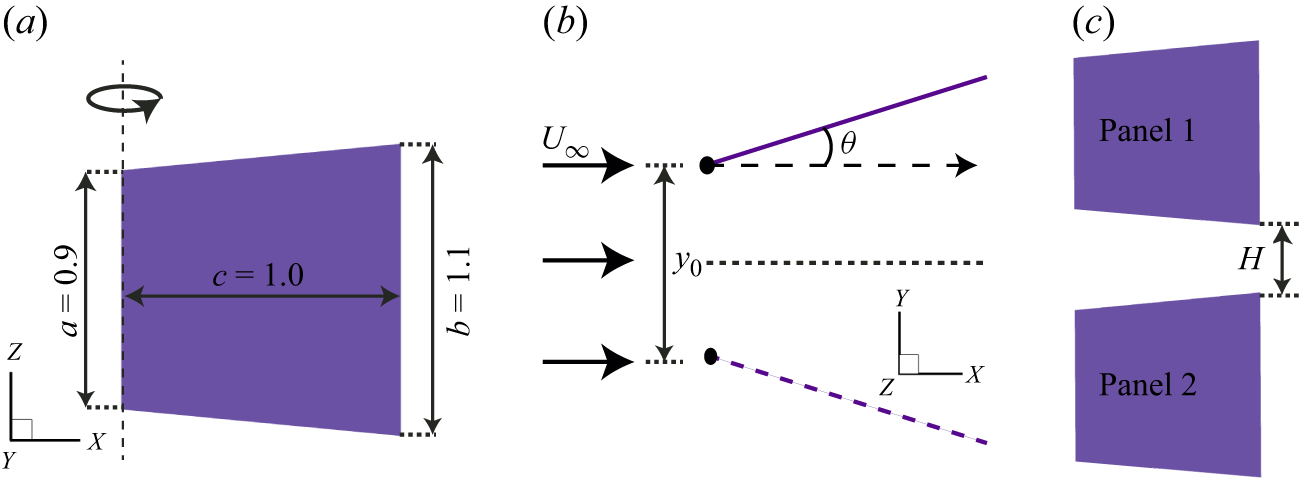


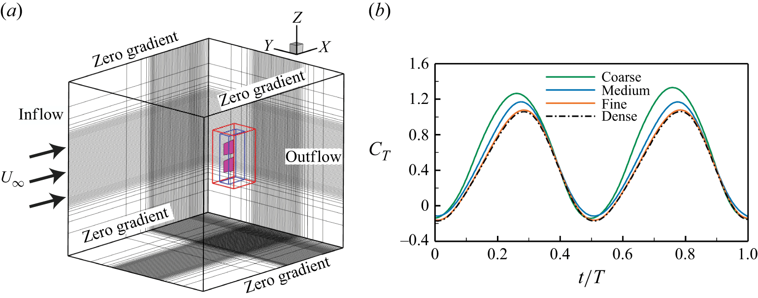


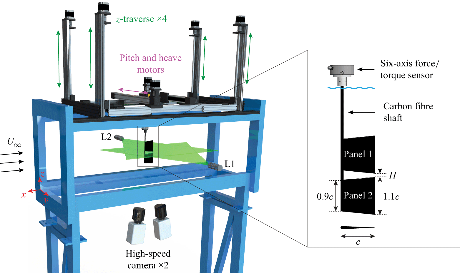

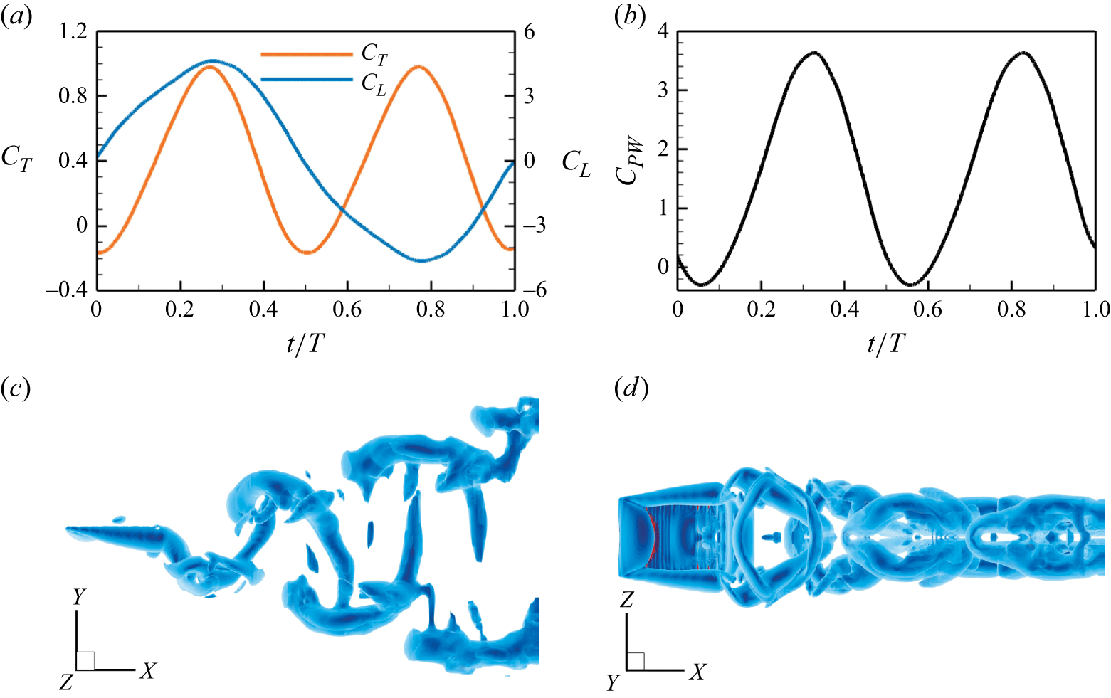


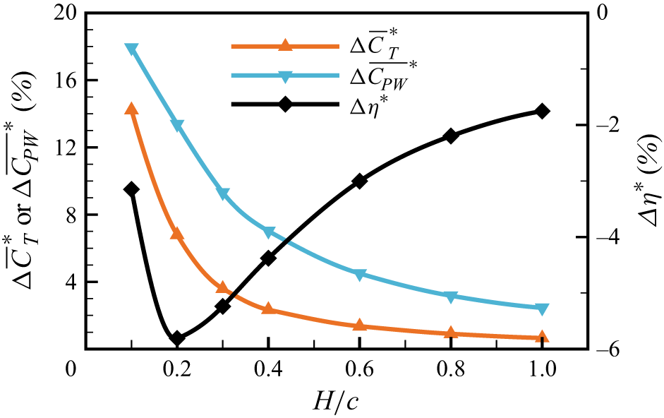


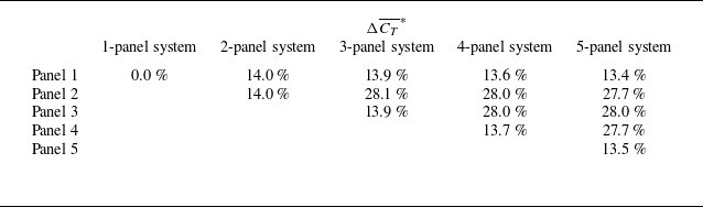


 Open access