


1. Introduction
The occurrence of ‘corner eddies’, a sequence of vortices of decreasing size and strength in the vicinity of a sharp edge, was initially revealed and analysed by Moffatt in the 1960s, in the context of continuum incompressible flows (Moffatt Reference Moffatt1964a , Reference Moffattb ). Ever since, follow-up continuum-flow investigations have been carried out (see Shankar & Deshpande (Reference Shankar and Deshpande2000) and works cited therein), considering the two-dimensional wedge-confined problem, as well as the three-dimensional cone-edge configuration. Both free-surface (external-flow-induced) and lid-driven set-ups have been examined, and the impacts of solid-wall dynamics and thermodynamic conditions have been investigated in detail, to examine their effect on the developed flow field.
While numerous works have focused on the problem at continuum-flow conditions, relatively few studies have analysed the effect of continuum breakdown on the appearance of corner recirculation. Considering lid-driven set-ups containing rarefied gases, the rectangle-shape hole geometry has been examined in several contributions (e.g. Qian & Wang Reference Qian and Wang2005; Naris & Valougeorgis Reference Naris and Valougeorgis2005; Kandemir & Kaya Reference Kandemir and Kaya2012; Wu, Reese & Zhang Reference Wu, Reese and Zhang2014; Wang et al. Reference Wang, Su, Zhu and Zhang2019; Nabapure & Murthy Reference Nabapure and R.C.Murthy2021), examining the impacts of cavity aspect ratio and surface conditions on vortical flow formation. Non-rectangular configurations, including circular (Zhu, Roohi & Ebrahimi Reference Zhu, Roohi and Ebrahimi2023) and other cavity shapes (Zakeri & Roohi Reference Zakeri and Roohi2021), have been similarly studied. In particular, triangular-cavity flows were considered (Roohi, Sahabi & Bagherzadeh Reference Roohi, Sahabi and Bagherzadeh2018), including a case where the cavity walls are stationary and fluid motion is induced through non-homogeneous wall temperatures (Mousivand & Roohi Reference Mousivand and Roohi2022).
In a separate list of studies, non-lid-driven (i.e. open) cavity flows, where fluid motion inside a pore is excited by external shear flow, were considered. Such set-ups are commonly encountered in grooved-wall geometries. Primarily, these are found in microchannel set-ups, where non-regular wall patterns are ubiquitous, as well as in outer-space flight vehicles, where design constraints result in non-smooth surface structures. In the former, flows passing in rough microchannels have been analysed, to study the impact of wall irregularities on channel permeability and cavity vortex formation (Tan, Kang & Wang Reference Tan, Kang and Wang2015; Rovenskaya & Croce Reference Rovenskaya and Croce2018; Zhang et al. Reference Zhang, Liu, Xu, Shan and Li2019; Sazhin Reference Sazhin2020). In the latter context of high-altitude flight, the effect of surface grooves on the vehicle overall aerodynamic efficiency (and, in particular, the drag force) has been examined (Guo & Luo Reference Guo and Luo2018; Nabapure, Singh & Kalluri Reference Nabapure, Singh and Kalluri2023; Shi et al. Reference Shi, Zhao, Su and Wu2023). Existing works have considered a variety of open-cavity configurations, including rectangular, semicircle and triangular (‘V-shape’) geometries, and examined a wide scope of rarefaction rates, encompassing near-continuum- to near-free-molecular-flow regimes (Guo & Luo Reference Guo and Luo2018; Jin et al. Reference Jin, Cheng, Wang and Wang2023; Jiang et al. Reference Jiang, Cai, Chen, Yuan, He and Liu2023; Ghamartale, Tsai & Tang Reference Ghamartale, Tsai and Tang2025). In this respect, a focus on the high-Knudsen-number limit is of particular interest, as it plays a vital role in high-altitude aerospace and microfluidic contexts, yet is relatively less explored compared with continuum-based studies. Evidently, the breakdown of continuum assumptions does not allow the application of conventional vortex analyses to study the problems in hand. A rigorous study of the generation of vortical flows at highly rarefied conditions, based on gas kinetic theory, is therefore of evident significance.
Almost entirely, all works studying rarefied gas cavity flows rely on numerical simulations. The prevailing scheme of solution applied is the direct simulation Monte Carlo (DSMC) method (Bird Reference Bird1994), which is routinely used for the description of rarefied gas flows. While DSMC calculations are known to converge to the solution of the Boltzmann kinetic equation (Wagner Reference Wagner1992), they require considerable computational efforts and lack the insight that may be gained through rigorous analyses. In relevance to the present topic, corner flow DSMC calculations are particularly challenging, as low flow speeds are expected, resulting in an inevitable decrease in the signal-to-noise ratio. This prohibits a detailed description of vortex formation near sharp corners, which is the main focus in corner flow studies.
In view of the above, the objective of the present work is to investigate the formation of corner circulation in the highly rarefied gas-flow regime. To this end, we consider the high-Knudsen-number limit of the two-dimensional gas flow developed in the vicinity of a sharp edge and driven by an external stream. Closed-form analysis is made in the free-molecular limit, where the impact of corner sidewall conditions is determined based on the Maxwell boundary model. The results obtained are compared with counterpart DSMC calculations, to test their validity and examine the effect of few molecular collisions (at large yet finite Knudsen numbers) on the vortical flow field. The impact of using other more elaborate gas–surface interaction models, namely the Cercignani–Lampis–Lord (CLL) law, is also discussed.
In the next section, the problem is formulated, for both circular (azimuthal) and straight outer flows. In § 3, the free-molecular solution is derived, and in § 4 the application of the DSMC numerical scheme is described. Our results are presented in § 5, and the work conclusions are discussed in § 6. Technical details are relegated to the appendices.
2. Statement of the problem
A schematic of the problem is presented in figure 1. Consider a perfect monatomic gas passing in the vicinity of a two-dimensional corner confined between solid walls of length $R^*$
(hereafter, asterisks denote dimensional quantities) with angle opening
$R^*$
(hereafter, asterisks denote dimensional quantities) with angle opening $0\lt 2\alpha \lt \pi$
. The outer flow is set at uniform density
$0\lt 2\alpha \lt \pi$
. The outer flow is set at uniform density $\rho _{\textit{out}}^*$
and temperature
$\rho _{\textit{out}}^*$
and temperature $T_{\textit{out}}^*$
. Using the marked Cartesian
$T_{\textit{out}}^*$
. Using the marked Cartesian $(x^*,y^*)$
or polar
$(x^*,y^*)$
or polar $(r^*,\theta )$
coordinate systems, two set-ups are examined, where the outer-flow velocity
$(r^*,\theta )$
coordinate systems, two set-ups are examined, where the outer-flow velocity $\boldsymbol{V}_{\textit{out}}^*$
is directed in either the azimuthal
$\boldsymbol{V}_{\textit{out}}^*$
is directed in either the azimuthal $\boldsymbol{\hat {\theta }}$
(figure 1
a) or vertical
$\boldsymbol{\hat {\theta }}$
(figure 1
a) or vertical $\boldsymbol{\hat {y}}$
(figure 1
b) direction. These represent the open-cavity counterparts of circular- and straight-wall lid-driven flows, respectively, that may be generated by the corresponding motion of a far-field wall, not modelled in the present work. Placing the axis origin at the corner edge, we seek to describe the steady gas motion inside the corner in the highly rarefied flow regime, where the corner length
$\boldsymbol{\hat {y}}$
(figure 1
b) direction. These represent the open-cavity counterparts of circular- and straight-wall lid-driven flows, respectively, that may be generated by the corresponding motion of a far-field wall, not modelled in the present work. Placing the axis origin at the corner edge, we seek to describe the steady gas motion inside the corner in the highly rarefied flow regime, where the corner length $R^*$
is assumed small compared with the gas mean free path.
$R^*$
is assumed small compared with the gas mean free path.
Schematic of the problem. A two-dimensional corner of length $R^*$
and angle opening
$R^*$
and angle opening $2\alpha$
is affected by an external uniform flow in the azimuthal
$2\alpha$
is affected by an external uniform flow in the azimuthal $\boldsymbol{\hat {\theta }}$
(a) or vertical
$\boldsymbol{\hat {\theta }}$
(a) or vertical $\boldsymbol{\hat {y}}$
(b) direction, set at density
$\boldsymbol{\hat {y}}$
(b) direction, set at density $\rho _{\textit{out}}^*$
, temperature
$\rho _{\textit{out}}^*$
, temperature $T_{\textit{out}}^*$
and speed
$T_{\textit{out}}^*$
and speed $V_{\textit{out}}^*$
.
$V_{\textit{out}}^*$
.

In the framework of gas kinetic theory and the present two-dimensional steady-flow set-up, the gas state is determined through its probability density function $f^*=f^*(r^*,\theta ,\boldsymbol{\xi }^*)$
, of finding a particle at position
$f^*=f^*(r^*,\theta ,\boldsymbol{\xi }^*)$
, of finding a particle at position $(r^*,\theta )$
with molecular velocity of about
$(r^*,\theta )$
with molecular velocity of about $\boldsymbol{\xi }^*$
. To analyse the velocity space, a cylindrical coordinate description is applied, putting
$\boldsymbol{\xi }^*$
. To analyse the velocity space, a cylindrical coordinate description is applied, putting $\boldsymbol{\xi }^*=(\xi ^*_r,\theta _\xi ,\xi _z^*)$
. Here,
$\boldsymbol{\xi }^*=(\xi ^*_r,\theta _\xi ,\xi _z^*)$
. Here, $\xi ^*_r\in [0,\infty )$
is the molecular velocity magnitude in the corner plane of motion,
$\xi ^*_r\in [0,\infty )$
is the molecular velocity magnitude in the corner plane of motion, $\theta _\xi$
is the corresponding in-plane velocity direction with respect to the positive
$\theta _\xi$
is the corresponding in-plane velocity direction with respect to the positive $x^*$
axis and
$x^*$
axis and $\xi _z^*\in (-\infty ,\infty )$
is the velocity component normal to the corner plane.
$\xi _z^*\in (-\infty ,\infty )$
is the velocity component normal to the corner plane.
Outside the corner (where $r^*\gt R^*$
), the flow is set at
$r^*\gt R^*$
), the flow is set at $f_{\textit{out}}^*=f_{\textit{out}}^*(r^*,\theta ,\boldsymbol{\xi }^*)$
, approaching a uniform Maxwellian at the indicated velocity
$f_{\textit{out}}^*=f_{\textit{out}}^*(r^*,\theta ,\boldsymbol{\xi }^*)$
, approaching a uniform Maxwellian at the indicated velocity $\boldsymbol{V}_{\textit{out}}^*$
, density
$\boldsymbol{V}_{\textit{out}}^*$
, density $\rho _{\textit{out}}^*$
and temperature
$\rho _{\textit{out}}^*$
and temperature $T_{\textit{out}}^*$
with increasing
$T_{\textit{out}}^*$
with increasing $r^*$
. At free-molecular conditions, gas particles entering the corner are strictly unaffected by outgoing particles, and therefore retain their far equilibrium Maxwellian. This condition becomes less effective with decreasing rarefaction rates. Yet, focusing on highly rarefied conditions, the impact of intermolecular interactions between outgoing and incoming particles is arguably minor, causing only a slight deviation from the above Maxwellian. We therefore apply the above-mentioned condition in subsequent DSMC calculations at high yet finite rarefaction rates. A more detailed study of the applicability of this approximation requires the simulation of the gas reservoir flow outside the corner. Such a study is skipped here, however, as similar investigations of counterpart gas systems at highly rarefied conditions (e.g. Ben-Adva & Manela Reference Ben-Adva and Manela2024) indicate that this effect is negligible at high rarefaction rates.
$r^*$
. At free-molecular conditions, gas particles entering the corner are strictly unaffected by outgoing particles, and therefore retain their far equilibrium Maxwellian. This condition becomes less effective with decreasing rarefaction rates. Yet, focusing on highly rarefied conditions, the impact of intermolecular interactions between outgoing and incoming particles is arguably minor, causing only a slight deviation from the above Maxwellian. We therefore apply the above-mentioned condition in subsequent DSMC calculations at high yet finite rarefaction rates. A more detailed study of the applicability of this approximation requires the simulation of the gas reservoir flow outside the corner. Such a study is skipped here, however, as similar investigations of counterpart gas systems at highly rarefied conditions (e.g. Ben-Adva & Manela Reference Ben-Adva and Manela2024) indicate that this effect is negligible at high rarefaction rates.
The specific form of $f_{\textit{out}}^*$
differs between the set-ups described in figure 1. For the circular-flow system shown in figure 1(a) we put
$f_{\textit{out}}^*$
differs between the set-ups described in figure 1. For the circular-flow system shown in figure 1(a) we put
 \begin{align} \nonumber &f_{\textit{circ}}^* \! \left (R^*,-\alpha \lt \theta \lt \alpha ,\xi ^*_r,\theta +\pi /2\lt \theta _\xi \lt \theta +3\pi /2,\xi _z^*\right ) \\ & \quad =\frac {\rho ^*_{\textit{out}}}{\pi ^{3/2}U^{*3}_{\textit{mp}}} \exp\! \left [-\frac {{{\xi ^*_r}^2+{V_{\textit{out}}^{*2}}}-2\xi _r^*V_{\textit{out}}^*\sin {(\theta _\xi -\theta )+{\xi _z^*}^2}}{U^{*2}_{\textit{mp}}}\right ]\!, \end{align}
whereas for the straight-outer-flow case in figure 1(b) we set
 \begin{align} \nonumber &f^*_{\textit{straight}}\! \left (R^*\cos \alpha/ \cos \theta,-\alpha \lt \theta \lt \alpha ,\xi _r^*,\pi /2\lt \theta _\xi \lt 3\pi /2,\xi _z^* \right ) \\ & \quad =\frac {\rho ^*_{\textit{out}}}{\pi ^{3/2}U^{*3}_{\textit{mp}}}\exp\! \left [-\frac {{{\xi _r^*}^2+{V^{*2}_{\textit{out}}}}-2\xi _r^*V^*_{\textit{out}}\sin {\theta _\xi +{\xi _z^*}^2}}{U^{*2}_{\textit{mp}}}\right ]\!. \end{align}
In (2.1) and (2.2), $U^*_{\textit{mp}}=(2\mathcal{R}_g^*T^*_{\textit{out}})^{1/2}$
denotes the most probable speed of a gas particle at the outer-flow temperature, where
$U^*_{\textit{mp}}=(2\mathcal{R}_g^*T^*_{\textit{out}})^{1/2}$
denotes the most probable speed of a gas particle at the outer-flow temperature, where $\mathcal{R}^*_g$
is the specific gas constant.
$\mathcal{R}^*_g$
is the specific gas constant.
To model gas–surface interactions of the gas particles with the corner solid walls, we apply the prevailing Maxwell condition (Sone Reference Sone2007):
 \begin{align} &\nonumber f^*\! \left (0\lt r^*\le R^*,\theta =\pm \alpha ,\boldsymbol{\xi }^*\boldsymbol{\cdot }\boldsymbol{\hat {n}}\gt 0\right ) \\ & \quad =\beta \frac {\rho ^*_\pm (r^*)}{\pi ^{3/2}U^{*3}_{\textit{mp}_\pm }}\exp\! {\left [-\frac {{\xi ^*}^2}{U^{*2}_{\textit{mp}_\pm }}\right ]} + (1-\beta ) f^*(r^*,\pm \alpha ,\boldsymbol{\xi }^*-2(\boldsymbol{\xi }^*\boldsymbol{\cdot }\boldsymbol{\hat {n}})\boldsymbol{\hat {n}}), \end{align}
where the relative $\beta$
and
$\beta$
and $(1-\beta )$
parts of the gas molecules are emitted diffusely and specularly, respectively, at each point along the boundaries. Here,
$(1-\beta )$
parts of the gas molecules are emitted diffusely and specularly, respectively, at each point along the boundaries. Here, $\boldsymbol{\hat {n}}$
is a unit vector directed normal to each wall and into the corner domain and
$\boldsymbol{\hat {n}}$
is a unit vector directed normal to each wall and into the corner domain and $\rho ^*_\pm (r^*)$
are as yet unknown functions associated with the mass flux of particles reflected from the surfaces
$\rho ^*_\pm (r^*)$
are as yet unknown functions associated with the mass flux of particles reflected from the surfaces $\theta =\pm \alpha$
, respectively. Additionally,
$\theta =\pm \alpha$
, respectively. Additionally, $U^*_{{mp}_\pm }=(2\mathcal{R}_g^*T^*_\pm )^{1/2}$
denotes the most probable speed of gas particles at the corner wall temperatures
$U^*_{{mp}_\pm }=(2\mathcal{R}_g^*T^*_\pm )^{1/2}$
denotes the most probable speed of gas particles at the corner wall temperatures $T^*_\pm$
. We hereafter assume that the corner surfaces are isothermal and maintained at the reference outer-flow temperature; thus
$T^*_\pm$
. We hereafter assume that the corner surfaces are isothermal and maintained at the reference outer-flow temperature; thus $T^*_\pm =T^*_{\textit{out}}$
and
$T^*_\pm =T^*_{\textit{out}}$
and $U^*_{{mp}_\pm }=U^*_{\textit{mp}}$
.
$U^*_{{mp}_\pm }=U^*_{\textit{mp}}$
.
Describing the $\beta =1$
and
$\beta =1$
and $\beta =0$
limit cases in (2.3), the former diffuse scattering occurs over rough surfaces, where the colliding particles attain thermal equilibrium with their reflecting boundaries. Specular (
$\beta =0$
limit cases in (2.3), the former diffuse scattering occurs over rough surfaces, where the colliding particles attain thermal equilibrium with their reflecting boundaries. Specular ( $\beta =0$
) interactions take place where the incident molecules collide with a solid surface and rebound elastically as if hitting a perfectly smooth wall. While none of these idealised scenarios exists in reality, it is commonly accepted that wall reflections from realistic surfaces may be described as a combination of diffuse and specular interactions, as formulated in (2.3). In particular, the practical realisation of nearly smooth walls, analysed in detail below, has been highlighted in a series of experimental investigations, showing close agreement between laboratory measurements and Maxwell-based theoretical predictions with
$\beta =0$
) interactions take place where the incident molecules collide with a solid surface and rebound elastically as if hitting a perfectly smooth wall. While none of these idealised scenarios exists in reality, it is commonly accepted that wall reflections from realistic surfaces may be described as a combination of diffuse and specular interactions, as formulated in (2.3). In particular, the practical realisation of nearly smooth walls, analysed in detail below, has been highlighted in a series of experimental investigations, showing close agreement between laboratory measurements and Maxwell-based theoretical predictions with $\beta \ll 1$
(Honig & Ducker Reference Honig and Ducker2010; Bowles & Ducker Reference Bowles and Ducker2011; Seo & Ducker Reference Seo and Ducker2013, Reference Seo and Ducker2014; Lei & McKenzie Reference Lei and McKenzie2015; Yousefi-Nasab, Safdari & Karimi-Sabet Reference Yousefi-Nasab, Safdari and Karimi-Sabet2024). Noting the dominant effect of gas-surface interaction on the flow field obtained at highly rarefied conditions, we additionally examine the application of the more elaborate CLL kernel (Cercignani & Lampis Reference Cercignani and Lampis1971; Lord Reference Lord1991) on the results in § 5.4.2. Yet, our discussion focuses primarily on the Maxwell condition, due to its common use and relative simplicity, which allows for the closed-form analysis carried out below.
$\beta \ll 1$
(Honig & Ducker Reference Honig and Ducker2010; Bowles & Ducker Reference Bowles and Ducker2011; Seo & Ducker Reference Seo and Ducker2013, Reference Seo and Ducker2014; Lei & McKenzie Reference Lei and McKenzie2015; Yousefi-Nasab, Safdari & Karimi-Sabet Reference Yousefi-Nasab, Safdari and Karimi-Sabet2024). Noting the dominant effect of gas-surface interaction on the flow field obtained at highly rarefied conditions, we additionally examine the application of the more elaborate CLL kernel (Cercignani & Lampis Reference Cercignani and Lampis1971; Lord Reference Lord1991) on the results in § 5.4.2. Yet, our discussion focuses primarily on the Maxwell condition, due to its common use and relative simplicity, which allows for the closed-form analysis carried out below.
To render the problem dimensionless, we scale the position by the corner wall length $R^*$
, the velocity by the outer-temperature-based most probable molecular speed
$R^*$
, the velocity by the outer-temperature-based most probable molecular speed $U^*_{\textit{mp}}$
and the density and temperature by
$U^*_{\textit{mp}}$
and the density and temperature by $\rho ^*_{\textit{out}}$
and
$\rho ^*_{\textit{out}}$
and $T^*_{\textit{out}}$
, respectively. The system non-dimensional description is subsequently governed by the outer-flow reduced velocity
$T^*_{\textit{out}}$
, respectively. The system non-dimensional description is subsequently governed by the outer-flow reduced velocity $V_{\textit{out}}$
, the corner semi-angle
$V_{\textit{out}}$
, the corner semi-angle $\alpha$
and the wall accommodation coefficient
$\alpha$
and the wall accommodation coefficient $\beta$
. In addition, the gas mean Knudsen number is introduced:
$\beta$
. In addition, the gas mean Knudsen number is introduced:
 \begin{equation} \textit{Kn}=\lambda ^*/R^*, \end{equation}
where $\lambda ^*$
is the mean free path of a gas molecule at the outer-flow conditions. Assuming a hard-sphere gas model,
$\lambda ^*$
is the mean free path of a gas molecule at the outer-flow conditions. Assuming a hard-sphere gas model, $\lambda ^*=m^*/(\pi \sqrt {2}\rho _{\textit{out}}^*d^{*2})$
, where
$\lambda ^*=m^*/(\pi \sqrt {2}\rho _{\textit{out}}^*d^{*2})$
, where $m^*$
and
$m^*$
and $d^*$
denote the gas molecular mass and diameter, respectively (Sone Reference Sone2007).
$d^*$
denote the gas molecular mass and diameter, respectively (Sone Reference Sone2007).
In what follows, we first analyse the free-molecular problem, where $\textit{Kn}\rightarrow \infty$
. Considering steady flow conditions, the cases of specular and diffuse wall reflections are studied separately, yielding explicit solutions for the collisionless flow regime in the set-ups described in figures 1(a) and 1(b). The application of the DSMC scheme, used to analyse the problem at large yet finite Knudsen numbers, is described in a subsequent section.
$\textit{Kn}\rightarrow \infty$
. Considering steady flow conditions, the cases of specular and diffuse wall reflections are studied separately, yielding explicit solutions for the collisionless flow regime in the set-ups described in figures 1(a) and 1(b). The application of the DSMC scheme, used to analyse the problem at large yet finite Knudsen numbers, is described in a subsequent section.
3. The free-molecular limit
Assuming $\textit{Kn}\rightarrow \infty$
and steady flow conditions, the gas kinetic problem is governed by the collisionless two-dimensional time-independent Boltzmann equation:
$\textit{Kn}\rightarrow \infty$
and steady flow conditions, the gas kinetic problem is governed by the collisionless two-dimensional time-independent Boltzmann equation:
 \begin{equation} \boldsymbol{\xi } \boldsymbol{\cdot }\boldsymbol{\nabla \!}f=0, \end{equation}
stating that $f=f(r,\theta ,\boldsymbol{\xi })$
remains unchanged along ‘free-flight’ particle trajectories in the absence of molecular collisions. Variations in the probability density function may therefore occur solely due to particle–surface interactions, governed by the scaled form of (2.3):
$f=f(r,\theta ,\boldsymbol{\xi })$
remains unchanged along ‘free-flight’ particle trajectories in the absence of molecular collisions. Variations in the probability density function may therefore occur solely due to particle–surface interactions, governed by the scaled form of (2.3):
 \begin{align} f\!\left (0\lt r\le 1,\theta =\pm \alpha ,\boldsymbol{\xi }\boldsymbol{\cdot }\boldsymbol{\hat {n}}\gt 0\right )= \beta \ \frac {\rho _\pm (r)}{\pi ^{3/2}}\exp {\big [-\xi ^2\big ]} + (1-\beta ) f(r,\pm \alpha ,\boldsymbol{\xi }-2(\boldsymbol{\xi }\boldsymbol{\cdot }\boldsymbol{\hat {n}})\boldsymbol{\hat {n}}). \end{align}
The solid-wall condition in (3.2) is supplemented by the non-dimensional counterpart of (2.1) or (2.2), prescribing the outer-flow state. In what follows, the free-molecular problem is analysed separately for the cases of fully specular ( $\beta =0$
, § 3.1) and fully diffuse (
$\beta =0$
, § 3.1) and fully diffuse ( $\beta =1$
, § 3.2) configurations. Discussion of the combined specular-diffuse (
$\beta =1$
, § 3.2) configurations. Discussion of the combined specular-diffuse ( $\beta \neq 0,1$
) set-up, obtained through superposition of the above two limits, is deferred to § 5.4.1.
$\beta \neq 0,1$
) set-up, obtained through superposition of the above two limits, is deferred to § 5.4.1.
Once the probability density function has been obtained, the hydrodynamic fields are calculated via appropriate quadratures over the molecular velocity space (Sone Reference Sone2007). Specifically, the density $\rho (r,\theta )$
, radial and azimuthal velocity components
$\rho (r,\theta )$
, radial and azimuthal velocity components $u_r(r,\theta )$
and
$u_r(r,\theta )$
and $u_\theta (r,\theta )$
, respectively, and pressure
$u_\theta (r,\theta )$
, respectively, and pressure $p(r,\theta )$
fields are given by
$p(r,\theta )$
fields are given by
 \begin{align} \nonumber &\rho = \int _{-\infty }^{\infty } f{\rm d}\boldsymbol{\xi } \ \ ,\ \ u_r = \frac {1}{\rho }\int _{-\infty }^{\infty }\xi _r \cos {(\theta _\xi -\theta )} f {\rm d}\boldsymbol{\xi } \ \ , \ \ u_\theta = \frac {1}{\rho }\int _{-\infty }^{\infty }\xi _r\sin {(\theta _\xi -\theta )} f {\rm d}\boldsymbol{\xi } \\ & \quad {\rm and} \quad p =\frac {2}{3} \int _{-\infty }^{\infty }\left (\left (u_r-\xi _r \cos {(\theta _\xi -\theta )}\right )^2+\left (u_\theta -\xi _r\sin {(\theta _\xi -\theta )}\right )^2+\xi _z^2\right )f{\rm d}\boldsymbol{\xi } , \end{align}
where ${\rm d}\boldsymbol{\xi }=\xi _r{\rm d}\xi _r{\rm d}\theta _\xi {\rm d}\xi _z$
. The temperature is computed via the scaled form of the equation of state for an ideal gas,
${\rm d}\boldsymbol{\xi }=\xi _r{\rm d}\xi _r{\rm d}\theta _\xi {\rm d}\xi _z$
. The temperature is computed via the scaled form of the equation of state for an ideal gas, $T(r,\theta )=p/\rho$
.
$T(r,\theta )=p/\rho$
.
3.1. Specular reflecting corner ( $\beta =0$
)
$\beta =0$
)

Considering a specular-wall corner set-up (see (3.2) with $\beta =0$
), the impermeability condition is satisfied identically. Thus, given a particle in-corner phase-space location
$\beta =0$
), the impermeability condition is satisfied identically. Thus, given a particle in-corner phase-space location $(r,\theta ,\xi _r,\theta _\xi ,\xi _z)$
, the specular-wall problem reduces to tracking its initial state at entering the corner, denoted by
$(r,\theta ,\xi _r,\theta _\xi ,\xi _z)$
, the specular-wall problem reduces to tracking its initial state at entering the corner, denoted by $(\bar {r},\bar {\theta },\bar {\xi }_r,\bar {\theta }_\xi ,\xi _z)$
(note that, while
$(\bar {r},\bar {\theta },\bar {\xi }_r,\bar {\theta }_\xi ,\xi _z)$
(note that, while $\bar {r}=1$
in the circular-outer-flow case,
$\bar {r}=1$
in the circular-outer-flow case, $\bar {r}=\cos \alpha /\cos \bar \theta$
in the straight-outer-flow problem; see figure 1). Clearly, since the magnitude of particle velocity does not change due to specular-wall interactions,
$\bar {r}=\cos \alpha /\cos \bar \theta$
in the straight-outer-flow problem; see figure 1). Clearly, since the magnitude of particle velocity does not change due to specular-wall interactions, $\bar {\xi }_r=\xi _r$
. Then, observing the change in particle trajectory direction with each specular-wall collision, we find
$\bar {\xi }_r=\xi _r$
. Then, observing the change in particle trajectory direction with each specular-wall collision, we find
 \begin{equation} \bar {\theta }_\xi = \begin{cases}(-1)^k(\theta _\xi -2\alpha k) , \quad \pi \lt \theta _\xi \lt 2\pi +\theta \\ (-1)^k(\theta _\xi +2\alpha k) , \quad 2\pi +\theta \lt \theta _\xi \lt 3\pi , \end{cases} \end{equation}
where $k$
marks the total number of wall collisions since the particle has entered the corner. The maximum number of wall collisions encountered by a particle at a given
$k$
marks the total number of wall collisions since the particle has entered the corner. The maximum number of wall collisions encountered by a particle at a given $\theta$
location is independent of
$\theta$
location is independent of $r$
, and given by
$r$
, and given by
 \begin{align} \begin{split} &n_{\textit{max}}^+(\theta ) = \left \lceil \frac {\pi +\theta -\alpha }{2\alpha }\right \rceil\! , \quad \pi \lt \theta _\xi \lt 2\pi +\theta \\ &n_{\textit{max}}^-(\theta ) = \left \lceil \frac {\pi -\theta -\alpha }{2\alpha }\right \rceil\! , \quad 2\pi +\theta \lt \theta _\xi \lt 3\pi , \end{split} \end{align}
where ‘ $+$
’ and ‘
$+$
’ and ‘ $-$
’ specify whether the last collision occurred with the
$-$
’ specify whether the last collision occurred with the $\theta =\alpha$
or
$\theta =\alpha$
or $\theta =-\alpha$
surfaces, respectively, and
$\theta =-\alpha$
surfaces, respectively, and $\lceil \boldsymbol{\cdot }\rceil$
is the integer ceiling of a number.
$\lceil \boldsymbol{\cdot }\rceil$
is the integer ceiling of a number.
Inspecting (3.5), it is observed that the maximum values of $n_{\textit{max}}^\pm (\theta )$
are achieved at the
$n_{\textit{max}}^\pm (\theta )$
are achieved at the $\theta =\pm \alpha$
solid walls, respectively, and are equal to
$\theta =\pm \alpha$
solid walls, respectively, and are equal to
 \begin{equation} \textit{max}\! \left \{n_{\textit{max}}^\pm (\theta )\right \} = n_{\textit{max}}^\pm (\pm \alpha ) = \left \lceil {\pi }/{2\alpha }\right \rceil \!. \end{equation}
In fact, the trajectories separating particle pathlines with different number of surface reflections are those passing through the wall-edge points, $(r,\theta )=(1,\pm \alpha )$
. The corresponding separating
$(r,\theta )=(1,\pm \alpha )$
. The corresponding separating $\theta _\xi$
directions are
$\theta _\xi$
directions are
 \begin{align} \begin{split} &\theta _{\xi ,\textit{sep}}^{+,k}(r,\theta ) = a^+\pi + \theta +\arctan {\left (\frac {\sin \left (\alpha (2k+1)-\theta \right )}{\cos \left (\alpha (2k+1)-\theta \right )-r}\right )} , \quad \pi \lt \theta _\xi \lt 2\pi +\theta \\ &\theta _{\xi ,\textit{sep}}^{-,k}(r,\theta ) = a^-\pi +\theta +\arctan {\left (\frac {\sin \left (\alpha (2k+1)+\theta \right )}{r-\cos \left (\alpha (2k+1)+\theta \right )}\right )} , \quad 2\pi +\theta \lt \theta _\xi \lt 3\pi . \end{split} \end{align}
In (3.7), each $k=0,1,\ldots , n_{\textit{max}}^{{+/-}}(\theta )-1$
value (see (3.5)) fixes the limit
$k=0,1,\ldots , n_{\textit{max}}^{{+/-}}(\theta )-1$
value (see (3.5)) fixes the limit $\theta _{\xi ,\textit{sep}}^{+/-,k}$
trajectory direction that separates particle pathlines with
$\theta _{\xi ,\textit{sep}}^{+/-,k}$
trajectory direction that separates particle pathlines with $k$
and
$k$
and $k+1$
wall collisions. Here, the integer constants
$k+1$
wall collisions. Here, the integer constants $a^+$
and
$a^+$
and $a^-$
are the
$a^-$
are the $\pi$
-multiples allotted such that
$\pi$
-multiples allotted such that $\theta _\xi$
is contained within the permitted
$\theta _\xi$
is contained within the permitted $(\pi ,2\pi +\theta )$
and
$(\pi ,2\pi +\theta )$
and $(2\pi +\theta ,3\pi )$
intervals, respectively.
$(2\pi +\theta ,3\pi )$
intervals, respectively.
To illustrate the interpretation of (3.7), figure 2 shows, for a $2\alpha =\pi /3$
specular corner set-up at
$2\alpha =\pi /3$
specular corner set-up at $(r,\theta )=(0.6,\pi /10)$
, an example for the
$(r,\theta )=(0.6,\pi /10)$
, an example for the $\theta _{\xi ,\textit{sep}}^{+,k}(r,\theta )$
division. Specifically, the
$\theta _{\xi ,\textit{sep}}^{+,k}(r,\theta )$
division. Specifically, the $\theta _{\xi ,\textit{sep}}^{+,0-2}\approx 1.26\pi ,1.69\pi ,1.93\pi$
and
$\theta _{\xi ,\textit{sep}}^{+,0-2}\approx 1.26\pi ,1.69\pi ,1.93\pi$
and $\theta _{\xi ,\textit{sep}}^{-,0-2}\approx 2.63\pi ,2.36\pi ,2.14\pi$
directions are depicted, respectively, by the arrowed lines (see (3.7)), together with indication of particle trajectories undergoing two (dashed blue curve) and three (dashed red curve) wall collisions. Here, particles arriving at
$\theta _{\xi ,\textit{sep}}^{-,0-2}\approx 2.63\pi ,2.36\pi ,2.14\pi$
directions are depicted, respectively, by the arrowed lines (see (3.7)), together with indication of particle trajectories undergoing two (dashed blue curve) and three (dashed red curve) wall collisions. Here, particles arriving at $(0.6,\pi /10)$
with in-plane velocity direction in the range
$(0.6,\pi /10)$
with in-plane velocity direction in the range $\theta _{\xi ,\textit{sep}}^{-,2} \lt \theta _\xi \lt \theta _{\xi ,\textit{sep}}^{-,1}$
have collided twice with the corner walls (where the recent collision occurred with the
$\theta _{\xi ,\textit{sep}}^{-,2} \lt \theta _\xi \lt \theta _{\xi ,\textit{sep}}^{-,1}$
have collided twice with the corner walls (where the recent collision occurred with the $\theta =-\alpha$
surface), whereas particles with
$\theta =-\alpha$
surface), whereas particles with $\theta _{\xi ,\textit{sep}}^{-,2}\lt \theta _\xi \lt \theta _{\xi ,\textit{sep}}^{+,2}$
have been reflected three times. At the chosen
$\theta _{\xi ,\textit{sep}}^{-,2}\lt \theta _\xi \lt \theta _{\xi ,\textit{sep}}^{+,2}$
have been reflected three times. At the chosen $\theta =\pi /10$
azimuthal direction,
$\theta =\pi /10$
azimuthal direction, $n_{\textit{max}}^\pm (\theta )=3$
, in accordance with (3.5).
$n_{\textit{max}}^\pm (\theta )=3$
, in accordance with (3.5).
Particle kinematics in a specular-wall corner: the arrow-marked lines show the $\theta _{\xi ,\textit{sep}}^{\pm ,k}$
(with
$\theta _{\xi ,\textit{sep}}^{\pm ,k}$
(with $k=0,1,2$
) directions (see (3.7)) calculated at
$k=0,1,2$
) directions (see (3.7)) calculated at $(r,\theta )=(0.6,\pi /10)$
in a
$(r,\theta )=(0.6,\pi /10)$
in a $2\alpha =\pi /3$
corner. The
$2\alpha =\pi /3$
corner. The $\theta =\pm \pi /6$
corner walls are marked by the bold lines and the point is indicated by the circle. The numbers in magenta are the numbers of wall collisions encountered by particles arriving at
$\theta =\pm \pi /6$
corner walls are marked by the bold lines and the point is indicated by the circle. The numbers in magenta are the numbers of wall collisions encountered by particles arriving at $(r,\theta )=(0.6,\pi /10)$
through the respective sections confined by the arrow-marked lines. The dashed red and blue curves show example trajectories with
$(r,\theta )=(0.6,\pi /10)$
through the respective sections confined by the arrow-marked lines. The dashed red and blue curves show example trajectories with $\theta _{\xi ,\textit{sep}}^{+,2}\lt \theta _\xi \lt \theta _{\xi ,\textit{sep}}^{-,2}$
(containing three wall collisions) and
$\theta _{\xi ,\textit{sep}}^{+,2}\lt \theta _\xi \lt \theta _{\xi ,\textit{sep}}^{-,2}$
(containing three wall collisions) and $\theta _{\xi ,\textit{sep}}^{-,2}\lt \theta _\xi \lt \theta _{\xi ,\textit{sep}}^{-,1}$
(having two surface reflections), respectively.
$\theta _{\xi ,\textit{sep}}^{-,2}\lt \theta _\xi \lt \theta _{\xi ,\textit{sep}}^{-,1}$
(having two surface reflections), respectively.

Once the sorting of particle trajectories at a given $(r,\theta )$
location is completed, the specular-wall
$(r,\theta )$
location is completed, the specular-wall $f^{\textit{(spec)}}(r,\theta ,\boldsymbol{\xi })$
is obtained as
$f^{\textit{(spec)}}(r,\theta ,\boldsymbol{\xi })$
is obtained as
 \begin{align} f^{{(\textit{spec})}}(r,\theta ,\boldsymbol{\xi }) = \begin{cases} f_{\textit{out}}(\bar {r},\bar {\theta },\xi _r,\theta _\xi ,\xi _z) \ \ \ \ \ \ \ \ \ \ \ \ \ \ \ \ \ \ \ \ \ \ \ \ \ \ ,\pi \lt \theta _\xi \lt \theta _{\xi ,\textit{sep}}^{+,0} \\ f_{\textit{out}}(\bar {r},\bar {\theta },\xi _r,(-1)^k(\theta _\xi -2\alpha k),\xi _z) \ \ \ \ ,\theta _{\xi ,\textit{sep}}^{+,k-1}\lt \theta _\xi \lt \theta _{\xi ,\textit{sep}}^{+,k} \ \ \ \ \ \ ,k=1,\ldots ,n_{\textit{max}}^{+}(\theta )-1 \\ f_{\textit{out}}(\bar {r},\bar {\theta },\xi _r,(-1)^k(\theta _\xi -2\alpha k),\xi _z) \ \ \ \ ,\theta _{\xi ,\textit{sep}}^{+,k-1}\lt \theta _\xi \lt 2\pi +\theta \ \ \ \ ,k=n_{\textit{max}}^+(\theta ) \\ f_{\textit{out}}(\bar {r},\bar {\theta },\xi _r,(-1)^k(\theta _\xi +2\alpha k),\xi _z) \ \ \ \ ,2\pi +\theta \lt \theta _\xi \lt \theta _{\xi ,\textit{sep}}^{-,k-1} \ \ \ \ ,k=n_{\textit{max}}^-(\theta ) \\ f_{\textit{out}}(\bar {r},\bar {\theta },\xi _r,(-1)^k(\theta _\xi +2\alpha k),\xi _z) \ \ \ \ ,\theta _{\xi ,\textit{sep}}^{-,k}\lt \theta _\xi \lt \theta _{\xi ,\textit{sep}}^{-,k-1} \ \ \ \ \ \ ,k=n_{\textit{max}}^{-}(\theta )-1, \ldots ,1 \\ f_{\textit{out}}(\bar {r},\bar {\theta },\xi _r,\theta _\xi ,\xi _z) \ \ \ \ \ \ \ \ \ \ \ \ \ \ \ \ \ \ \ \ \ \ \ \ \ \ ,\theta _{\xi ,\textit{sep}}^{-,0}\lt \theta _\xi \lt 3\pi , \\ \end{cases} \end{align}
where $f_{\textit{out}}$
differs between circular- and straight-outer-flow set-ups (or any other outer flow of interest), as specified by the non-dimensional counterparts of (2.1) and (2.2), respectively. The values of
$f_{\textit{out}}$
differs between circular- and straight-outer-flow set-ups (or any other outer flow of interest), as specified by the non-dimensional counterparts of (2.1) and (2.2), respectively. The values of $\bar {r}$
and
$\bar {r}$
and $\bar \theta$
similarly vary between the two configurations, as detailed in §§ 3.1.1 and 3.1.2.
$\bar \theta$
similarly vary between the two configurations, as detailed in §§ 3.1.1 and 3.1.2.
Once $f^{\textit{(spec)}}(r,\theta ,\boldsymbol{\xi })$
is known, the calculation of the hydrodynamic fields follows (3.3). All
$f^{\textit{(spec)}}(r,\theta ,\boldsymbol{\xi })$
is known, the calculation of the hydrodynamic fields follows (3.3). All $\xi _z$
and
$\xi _z$
and $\xi _r$
quadratures may be carried out in a closed form, yielding expressions containing the Gamma function. The integrations over
$\xi _r$
quadratures may be carried out in a closed form, yielding expressions containing the Gamma function. The integrations over $\theta _\xi$
are then evaluated numerically, requiring a minor computational effort.
$\theta _\xi$
are then evaluated numerically, requiring a minor computational effort.
3.1.1. Circular outer flow
In the circular-flow configuration, $\bar {r}=1$
. Scaling (2.1), we obtain
$\bar {r}=1$
. Scaling (2.1), we obtain
 \begin{equation} f_{\textit{out}}=f_{\textit{circ}}= \pi ^{-3/2}\exp \big [{-\xi _r}^2-V^2_{\textit{out}}+2\xi _r V_{\textit{out}}\sin {(\theta _\xi -\theta )}-\xi _z^2\big ], \end{equation}
where, in line with subsequent geometrical considerations,
 \begin{equation} \bar {\theta }= \begin{cases} (-1)^k(\theta _\xi -\pi -2\alpha k+\arcsin {(r\sin {(\theta _\xi -\theta )})}) ,\quad\pi \lt \theta _\xi \lt 2\pi +\theta \\ (-1)^k(\theta _\xi -\pi +2\alpha k+\arcsin {(r\sin {(\theta _\xi -\theta )})}) ,\quad2 \pi +\theta \lt \theta _\xi \lt 3\pi . \end{cases} \end{equation}
Substituting (3.9) and (3.10) together with $\bar {r}=1$
into (3.8), we find
$\bar {r}=1$
into (3.8), we find
 \begin{equation} f_{\textit{circ}}^{\textit{(spec)}}(r,\theta ,\boldsymbol{\xi }) =\pi ^{-3/2}\exp \big [{{-\xi _r}^2-V_{\textit{out}}^2}+(-1)^k2\xi _r V_{\textit{out}}r\sin (\theta _\xi -\theta )-\xi _z^2\big ], \end{equation}
where the value of $k$
, denoting the number of particle–wall collisions along its trajectory, is determined through (3.7).
$k$
, denoting the number of particle–wall collisions along its trajectory, is determined through (3.7).
3.1.2. Straight outer flow
In the straight-outer-flow set-up, $\bar {r}=\cos \alpha /\cos \bar {\theta }$
, and (cf. (2.2))
$\bar {r}=\cos \alpha /\cos \bar {\theta }$
, and (cf. (2.2))
 \begin{equation} f_{\textit{out}}=f_{\textit{straight}} =\pi ^{-3/2}\exp \big[{-\xi _r^2-V_{\textit{out}}^2}+2\xi _r V_{\textit{out}}\sin \theta _\xi -\xi _z^2\big ]. \end{equation}
Substituting (3.4) and (3.12) into (3.8) and carrying out some algebraic manipulations, we find
 \begin{align} f_{\textit{straight}}^{\textit{(spec)}}(r,\theta ,\boldsymbol{\xi }) = \begin{cases} \pi ^{-3/2}\exp\! \left [-\xi _r^2-V_{\textit{out}}^2+(-1)^k2\xi _r V_{\textit{out}}\sin {(\theta _\xi -2\alpha k)}-\xi _z^2\right ]\! ,\quad \pi \lt \theta _\xi \lt 2\pi +\theta \nonumber \\ \pi ^{-3/2}\exp\! \left [-\xi _r^2-V_{\textit{out}}^2+(-1)^k2\xi _r V_{\textit{out}}\sin {(\theta _\xi +2\alpha k)}-\xi _z^2\right ]\! ,\quad2\pi +\theta \lt \theta _\xi \lt 3\pi , \end{cases} \end{align}
where $k$
, as above, is the number of wall collisions for each
$k$
, as above, is the number of wall collisions for each $\theta _\xi$
, determined using (3.7).
$\theta _\xi$
, determined using (3.7).
3.2. Diffuse reflecting corner (
$\beta =1$
)

Setting $\beta =1$
in (3.2), the probability density function associated with each gas particle is governed by its most recent interaction with one of the corner (solid or free) surfaces. Recalling that the prescribed outer-flow and corner-wall temperatures are equal (see (2.3) et seq.), the expression for the scaled diffuse-wall probability density function
$\beta =1$
in (3.2), the probability density function associated with each gas particle is governed by its most recent interaction with one of the corner (solid or free) surfaces. Recalling that the prescribed outer-flow and corner-wall temperatures are equal (see (2.3) et seq.), the expression for the scaled diffuse-wall probability density function $f^{\textit{(diff)}}(r,\theta ,\boldsymbol{\xi })$
is
$f^{\textit{(diff)}}(r,\theta ,\boldsymbol{\xi })$
is
 \begin{equation} f^{\textit{(diff)}}(r,\theta ,\boldsymbol{\xi })= \begin{cases} \pi ^{-3/2}\rho _+(r_+)\exp\! \left [-\xi ^2 \right ]\! ,\quad \theta _{\xi ,\textit{sep}}^{+,0}\lt \theta _\xi \lt 2\pi +\theta \\ \pi ^{-3/2}\rho _-(r_-)\exp\! \left [-\xi ^2 \right ]\! ,\quad 2\pi +\theta \lt \theta _\xi \lt \theta _{\xi ,\textit{sep}}^{-,0} \\ f_{\textit{out}}(\bar {r},\bar {\theta },\boldsymbol{\xi }) ,\quad \pi \lt \theta _\xi \lt \theta _{\xi ,\textit{sep}}^{+,0} \quad \text{or} \quad \theta _{\xi ,\textit{sep}}^{-,0}\lt \theta _\xi \lt 3\pi , \end{cases} \end{equation}
where $r_\pm$
denote the point of recent reflection of the particle from the
$r_\pm$
denote the point of recent reflection of the particle from the $\theta =\pm \alpha$
boundary, respectively. The wall flux
$\theta =\pm \alpha$
boundary, respectively. The wall flux $\rho _\pm (r_\pm )$
functions are fixed through the impermeability condition along each of the solid corner surfaces, taking the form
$\rho _\pm (r_\pm )$
functions are fixed through the impermeability condition along each of the solid corner surfaces, taking the form
 \begin{equation} \int _{\boldsymbol{\xi }\boldsymbol{\cdot }\boldsymbol{\hat {n}}\gt 0}\boldsymbol{\xi }\boldsymbol{\cdot }\boldsymbol{\hat {n}}f(r,\pm \alpha ,\boldsymbol{\xi })\,{\rm d}\boldsymbol{\xi }+ \int _{\boldsymbol{\xi }\boldsymbol{\cdot }\boldsymbol{\hat {n}}\lt 0}\boldsymbol{\xi }\boldsymbol{\cdot }\boldsymbol{\hat {n}}f(r,\pm \alpha ,\boldsymbol{\xi })\,{\rm d}\boldsymbol{\xi }=0. \end{equation}
Here, the first and second integrals express the separate contributions of the outgoing and incoming particles to the macroscopic gas velocity normal to the surface, respectively. We next calculate the explicit form of this condition on each of the corner walls.
Considering the impermeability balance over the $\theta =\alpha$
surface and starting with the contribution of reflected particles, we substitute (3.14) into the first integral in (3.15), to obtain
$\theta =\alpha$
surface and starting with the contribution of reflected particles, we substitute (3.14) into the first integral in (3.15), to obtain
 \begin{equation} \int _{\boldsymbol{\xi }\boldsymbol{\cdot }\boldsymbol{\hat {n}}\gt 0}\xi _r\sin {(\theta _\xi -\alpha )}f(r,\alpha ,\boldsymbol{\xi })\,{\rm d}\boldsymbol{\xi }= -\frac {\rho _+(r)}{2\sqrt {\pi }}. \end{equation}
Then, the contribution of the incoming particles to the flux balance, accounted for by the second integral in (3.15), is
 \begin{align} \nonumber &{ \int _{\boldsymbol{\xi }\boldsymbol{\cdot }\boldsymbol{\hat {n}}\lt 0}\xi _r\sin (\theta _\xi -\alpha )f(r,\alpha,\boldsymbol{\xi })\,{\rm d}\boldsymbol{\xi }}= \frac {1}{4\sqrt {\pi }} \int _{\alpha +2\pi }^{\theta _{\xi ,\textit{sep}}^{-,0} } \rho _-\left (\frac {r\sin {(\theta _\xi -\alpha )}}{\sin {(\theta _\xi +\alpha )}}\right )\sin {(\theta _\xi -\alpha )}\,{\rm d}\theta _\xi \\ &\quad +\int _{-\infty }^\infty \int _0^\infty \int _\pi ^{\theta _{\xi ,\textit{sep}}^{+,0} } f_{\textit{out}}(\bar {r},\bar {\theta },\boldsymbol{\xi })\xi _r\sin {(\theta _\xi -\alpha )}\,{\rm d}\boldsymbol{\xi } \nonumber \\& \quad + \int _{-\infty }^\infty \int _0^\infty \int _{\theta _{\xi ,\textit{sep}}^{-,0}}^{3\pi } f_{\textit{out}}(\bar {r},\bar {\theta },\boldsymbol{\xi })\xi _r\sin {(\theta _\xi -\alpha )}\,{\rm d}\boldsymbol{\xi }, \end{align}
where the $\xi _z$
and
$\xi _z$
and $\xi _r$
quadratures for the particles arriving from the
$\xi _r$
quadratures for the particles arriving from the $\theta =-\alpha$
wall were computed analytically. Combining (3.16) and (3.17), we obtain the no-penetration condition over the
$\theta =-\alpha$
wall were computed analytically. Combining (3.16) and (3.17), we obtain the no-penetration condition over the $\theta =\alpha$
surface:
$\theta =\alpha$
surface:
 \begin{align} &\frac {\rho _+(r)}{2\sqrt {\pi }}- \frac {1}{4\sqrt {\pi }} \int _{\alpha +2\pi }^{\theta _{\xi ,\textit{sep}}^{-,0} } \rho _-\left (\frac {r\sin {(\theta _\xi -\alpha )}}{\sin {(\theta _\xi +\alpha )}}\right )\sin {(\theta _\xi -\alpha })\,{\rm d}\theta _\xi \nonumber \\ & \quad =\int _{-\infty }^\infty \int _0^\infty \int _\pi ^{\pi +\alpha } f_{\textit{out}}(\bar {r},\bar {\theta },\boldsymbol{\xi })\xi _r\sin {(\theta _\xi -\alpha })\,{\rm d}\boldsymbol{\xi } \nonumber \\ & \quad + \int _{-\infty }^\infty \int _0^\infty \int _{\theta _{\xi ,\textit{sep}}^{-,0}}^{3\pi } f_{\textit{out}}(\bar {r},\bar {\theta },\boldsymbol{\xi })\xi _r\sin {(\theta _\xi -\alpha })\, {\rm d}\boldsymbol{\xi }, \end{align}
with the outer-flow contribution expressed as the forcing terms on the right-hand side. A similar calculation over the $\theta =-\alpha$
wall yields the no-flux balance:
$\theta =-\alpha$
wall yields the no-flux balance:
 \begin{align} &\frac {\rho _-(r)}{2\sqrt {\pi }}+ \frac {1}{4\sqrt {\pi }}\int _{\theta _{\xi ,\textit{sep}}^{+,0}}^{2\pi -\alpha } \rho _+\left (\frac {r\sin {(\theta _\xi +\alpha )}}{\sin {(\theta _\xi -\alpha )}}\right )\sin {(\theta _\xi +\alpha })\,{\rm d}\theta _\xi \nonumber \\& \quad = -\int _{-\infty }^\infty \int _0^\infty \int _\pi ^{\theta _{\xi ,\textit{sep}}^{+,0} } f_{\textit{out}}(\bar {r},\bar {\theta },\boldsymbol{\xi })\xi _r\sin {(\theta _\xi +\alpha })\,{\rm d}\boldsymbol{\xi } \nonumber \\& \quad - \int _{-\infty }^\infty \int _0^\infty \int _{3\pi -\alpha }^{3\pi } f_{\textit{out}}(\bar {r},\bar {\theta },\boldsymbol{\xi })\xi _r\sin {(\theta _\xi +\alpha })\, {\rm d}\boldsymbol{\xi }. \end{align}
Equations (3.18)–(3.19) form a system of coupled non-homogeneous integral balances for the wall-flux functions $\rho _+(r)$
and
$\rho _+(r)$
and $\rho _-(r)$
. Once
$\rho _-(r)$
. Once $f_{\textit{out}}$
is specified for either circular or straight outer flows (see (3.9) or (3.12), respectively), the problem is solved numerically by discretising the fluxes at equally spaced
$f_{\textit{out}}$
is specified for either circular or straight outer flows (see (3.9) or (3.12), respectively), the problem is solved numerically by discretising the fluxes at equally spaced $N_w$
points along the corner boundaries. The integral terms are evaluated using the trapezoidal rule with
$N_w$
points along the corner boundaries. The integral terms are evaluated using the trapezoidal rule with $N_{\theta _\xi }\approx 10^4$
points, yielding a system of
$N_{\theta _\xi }\approx 10^4$
points, yielding a system of $2N_w$
linear non-homogeneous algebraic equations, inverted using a MATLAB subroutine. Our calculations indicate that converged results (with an error
$2N_w$
linear non-homogeneous algebraic equations, inverted using a MATLAB subroutine. Our calculations indicate that converged results (with an error $\lesssim 0.1\,\%$
) are obtained for
$\lesssim 0.1\,\%$
) are obtained for $N_w\approx 10^3$
discretisation points. This requires a negligible computational effort compared with the molecular simulation calculation described in the next section.
$N_w\approx 10^3$
discretisation points. This requires a negligible computational effort compared with the molecular simulation calculation described in the next section.
4. The DSMC scheme
The DSMC method is the most prevalent scheme for analysing rarefied gas flows (Bird Reference Bird1994), and is known to provide results that converge to the solution of the Boltzmann equation (Wagner Reference Wagner1992). In its numerical realisation, the physical domain is divided into computational cells and simulation particles are introduced. With each simulation particle representing a large number of real particles, the simulation evolves in time in discrete steps, and particle motions are divided into free-flight and collision parts. In the former, the particles are translated according to their instantaneous velocity. In the latter, collisions are treated in a stochastic manner, following a chosen collision scheme.
In the present work, we applied the two-dimensional Visual DSMC program for two-dimensional flows to analyse the micro-corner problem at finite large Knudsen numbers. By doing so we aim at validating the above free-molecular solution and describe its breakdown with decreasing rarefaction rate. The software has been frequently used as a reliable tool for computing rarefied gas flows, including recent investigations on supersonic jet expansion (Patel Reference Patel2021), compression corner detachment (Li, Yu & Bao Reference Li, Yu and Bao2021), shock-wave detection (Kovacs et al. Reference Kovacs, Passaggaia, Mazellier and Lago2022), microscale reaction–diffusion models (Zhang & Wang Reference Zhang and Wang2023) and curved microchannel flows (Ben-Adva & Manela Reference Ben-Adva and Manela2024). Applying the commonly used ‘no-time-counter’ collision scheme (Bird Reference Bird1994), we consider a hard-sphere gas model of molecular interaction. In each calculation, the micro-corner was initially set in vacuum. Particles were then allowed to enter the computational domain through its outer (circular or straight) open boundary, carrying their Maxwellian outer-flow equilibrium distribution. Outgoing particles were removed from the calculation, and the simulation was followed until a steady state was achieved. In line with the software settings, the simulation time step was taken as $1/3$
of the mean collision time and the mesh was locally adapted such that each computational cell size was considerably smaller than the local mean free path. Considering the large Knudsen numbers considered, a number of
$1/3$
of the mean collision time and the mesh was locally adapted such that each computational cell size was considerably smaller than the local mean free path. Considering the large Knudsen numbers considered, a number of $\approx 2\times 10^6$
particles and
$\approx 2\times 10^6$
particles and $\approx 1\times 10^5$
collision cells proved sufficient to ensure reliably converged results. A single run lasted several hours using an Intel 16-core i7 processor machine, marking a computational effort that is considerably more demanding than the above-described free-molecular calculation.
$\approx 1\times 10^5$
collision cells proved sufficient to ensure reliably converged results. A single run lasted several hours using an Intel 16-core i7 processor machine, marking a computational effort that is considerably more demanding than the above-described free-molecular calculation.
Considering the inevitably low flow speeds characterising the corner edge flow, the application of the DSMC scheme in the present context is particularly challenging, due to the non-large signal-to-noise ratio that typically appears in the results. This, in turn, hinders a detailed description and identification of the vortical flow structure obtained in the vicinity of the corner origin, which is a main focus of the current analysis. To reduce the simulation noise level, averaging over several separate calculations was carried out. Yet, the advantage of the above-described collisionless flow analysis, providing a noise-free description of the high-Knudsen-number flow regime, is evident.
The error margins in DSMC calculations may be assessed either through comparison of high-Knudsen-number computations with the analytical free-molecular solution, or by quantifying the relative change in results via an increase in the number of computational cells and particles. In both cases, our calculations indicate that a doubling of the number of particles and collision cells over the above-reported values impacts the density and temperature fields by less than $1\,\%$
. Larger deviations of up to
$1\,\%$
. Larger deviations of up to $\lesssim 5\,\%$
have been observed in the velocity field, a consequence of the characteristically small speed values present in the vicinity of the corner origin.
$\lesssim 5\,\%$
have been observed in the velocity field, a consequence of the characteristically small speed values present in the vicinity of the corner origin.
5. Results
The non-dimensional problem stated in § 2 is governed by the flow Knudsen number $\textit{Kn}$
, the outer-flow velocity magnitude
$\textit{Kn}$
, the outer-flow velocity magnitude $V_{\textit{out}}$
and type (circular or straight), the corner angle
$V_{\textit{out}}$
and type (circular or straight), the corner angle $2\alpha$
and the surface wall conditions. Focusing primarily on the free-molecular (
$2\alpha$
and the surface wall conditions. Focusing primarily on the free-molecular ( $\textit{Kn}\rightarrow \infty$
) limit, we make use of the ballistic solution to rationalise the effect of problem parameters on the flow pattern in specular-corner (§ 5.1) and diffuse-corner (§ 5.2) set-ups. We then examine the impact of molecular collisions on the system behaviour using DSMC calculations, to validate the free-molecular description and inspect its breakdown with decreasing rarefaction.
$\textit{Kn}\rightarrow \infty$
) limit, we make use of the ballistic solution to rationalise the effect of problem parameters on the flow pattern in specular-corner (§ 5.1) and diffuse-corner (§ 5.2) set-ups. We then examine the impact of molecular collisions on the system behaviour using DSMC calculations, to validate the free-molecular description and inspect its breakdown with decreasing rarefaction.
5.1. Specular-wall corner
Starting with the specular-corner ( $\beta =0$
) set-up, figure 3 presents the kinematic and dynamic divisions of the
$\beta =0$
) set-up, figure 3 presents the kinematic and dynamic divisions of the $(\alpha ,V_{\textit{out}})$
plane of parameters into domains with different number of maximal wall collisions (
$(\alpha ,V_{\textit{out}})$
plane of parameters into domains with different number of maximal wall collisions ( $n_{\textit{max}}(\alpha )$
) and vortical structures in the free-molecular flow regime. The dashed vertical lines confine the zones with different
$n_{\textit{max}}(\alpha )$
) and vortical structures in the free-molecular flow regime. The dashed vertical lines confine the zones with different $n_{\textit{max}}(\alpha )$
values, and the blue, light blue, green and yellow subdomains mark parameter areas with one, two, three and four vortices, respectively. The numbers and numbers in parentheses denote, in each zone, the number of vortices
$n_{\textit{max}}(\alpha )$
values, and the blue, light blue, green and yellow subdomains mark parameter areas with one, two, three and four vortices, respectively. The numbers and numbers in parentheses denote, in each zone, the number of vortices $n_{{vor}}$
and the values of
$n_{{vor}}$
and the values of $n_{\textit{max}}(\alpha )$
, respectively. The results for the cases of circular and straight outer flows are shown in figures 3(a) and 3(b), respectively, and are based on the solution derived in § 3.1.
$n_{\textit{max}}(\alpha )$
, respectively. The results for the cases of circular and straight outer flows are shown in figures 3(a) and 3(b), respectively, and are based on the solution derived in § 3.1.
Free-molecular kinematic and dynamic division of the $(\alpha ,V_{\textit{out}})$
plane for a specular-wall corner into domains of different numbers of maximal wall collisions (
$(\alpha ,V_{\textit{out}})$
plane for a specular-wall corner into domains of different numbers of maximal wall collisions ( $n_{\textit{max}}(\alpha )$
) and vortical structures. The dashed vertical lines confine the zones with different
$n_{\textit{max}}(\alpha )$
) and vortical structures. The dashed vertical lines confine the zones with different $n_{\textit{max}}(\alpha )$
values, and the blue, light blue, green and yellow zones mark parameter subdomains with one, two, three and four vortices, respectively. The numbers and numbers in parentheses denote the number of vortices and the value of
$n_{\textit{max}}(\alpha )$
values, and the blue, light blue, green and yellow zones mark parameter subdomains with one, two, three and four vortices, respectively. The numbers and numbers in parentheses denote the number of vortices and the value of $n_{\textit{max}}(\alpha )$
in each zone, respectively. (a) Results for circular outer flow and (b) counterpart data for straight external flow. The red circle, triangle and cross notations indicate the parameter combinations referred to in figures 4, 6 and 11, respectively.
$n_{\textit{max}}(\alpha )$
in each zone, respectively. (a) Results for circular outer flow and (b) counterpart data for straight external flow. The red circle, triangle and cross notations indicate the parameter combinations referred to in figures 4, 6 and 11, respectively.

Making use of its common definition, we describe a two-dimensional vortex as a region in the flow field where the fluid revolves about a fixed point. In the free-molecular regime, as well as in other finite-Knudsen-number set-ups, we apply this definition to the gas macroscopic velocity field, calculated via quadrature of the velocity distribution function over the microscopic velocity space, as specified in (3.3). To identify vortices, as discussed below, we seek for stagnation points along the walls as indicators for a change in the velocity direction. This is qualitatively different from the continuum regime, where the no-slip restriction implies that the gas is stagnant along solid boundaries. Advantageously, the high accuracy of the analytical free-molecular solution allows us to resolve the macroscopic flow streamlines and identify the closed recirculation zones with good precision.
Remarkably, the system kinematic (microscopic) and dynamic (macroscopic) descriptions are closely linked. This is unequivocally manifested in figure 3 through the common $\alpha$
angles separating between set-ups with different maximum number of particle–wall collisions (corresponding to corner angles
$\alpha$
angles separating between set-ups with different maximum number of particle–wall collisions (corresponding to corner angles $2\alpha ={\pi }/{n_{\textit{max}}}$
, where
$2\alpha ={\pi }/{n_{\textit{max}}}$
, where $n_{\textit{max}}=3,4,\ldots$
; cf. (3.6)) and different number of corner vortices. In line with (3.6), the
$n_{\textit{max}}=3,4,\ldots$
; cf. (3.6)) and different number of corner vortices. In line with (3.6), the $\alpha$
intervals pertaining to different
$\alpha$
intervals pertaining to different $n_{\textit{max}}$
values diminish with decreasing
$n_{\textit{max}}$
values diminish with decreasing $\alpha$
. At sufficiently low
$\alpha$
. At sufficiently low $V_{\textit{out}}$
speeds (
$V_{\textit{out}}$
speeds ( $V_{\textit{out}}\lesssim 1$
),
$V_{\textit{out}}\lesssim 1$
), $n_{\textit{max}}$
variations are accompanied by an alternating change in
$n_{\textit{max}}$
variations are accompanied by an alternating change in $n_{{vor}}$
between one (for odd
$n_{{vor}}$
between one (for odd $n_{\textit{max}}$
) and two (for even
$n_{\textit{max}}$
) and two (for even $n_{\textit{max}}$
) vortices. At a fixed (and sufficiently low) value of
$n_{\textit{max}}$
) vortices. At a fixed (and sufficiently low) value of $\alpha$
, an increase in
$\alpha$
, an increase in $V_{\textit{out}}$
yields the appearance of multiple vortical structures, which are added in pairs. These features are common in both circular- and straight-flow configurations, indicating that the increase in
$V_{\textit{out}}$
yields the appearance of multiple vortical structures, which are added in pairs. These features are common in both circular- and straight-flow configurations, indicating that the increase in $n_{{vor}}$
occurs characteristically at lower values of
$n_{{vor}}$
occurs characteristically at lower values of $V_{\textit{out}}$
for lower
$V_{\textit{out}}$
for lower $\alpha$
.
$\alpha$
.
To visualise some of the flow fields described above, figure 4 presents free-molecular velocity amplitude colourmaps and streamlines in a specular-wall corner at the indicated combinations of $\alpha$
and
$\alpha$
and $V_{\textit{out}}$
, also marked by circles in figure 3. Figure 4(a–d) show characteristically low
$V_{\textit{out}}$
, also marked by circles in figure 3. Figure 4(a–d) show characteristically low $V_{\textit{out}}=0.1$
results for circular (figure 4
a,c) and straight (figure 4
b,d) outer-flow configurations, at
$V_{\textit{out}}=0.1$
results for circular (figure 4
a,c) and straight (figure 4
b,d) outer-flow configurations, at $\alpha$
values that are slightly below and above
$\alpha$
values that are slightly below and above $\alpha (n_{\textit{max}}=6)=15^\circ$
. Figures 4(e) and 4(f) then show counterpart data at
$\alpha (n_{\textit{max}}=6)=15^\circ$
. Figures 4(e) and 4(f) then show counterpart data at $\alpha =14.9^\circ$
and large
$\alpha =14.9^\circ$
and large $V_{\textit{out}}=2.4$
, for the circular- and straight-flow set-ups, respectively.
$V_{\textit{out}}=2.4$
, for the circular- and straight-flow set-ups, respectively.
Free-molecular velocity amplitude colourmaps and streamlines in a specular-wall corner at the indicated values of the corner semi-angle $\alpha$
and outer-flow speed
$\alpha$
and outer-flow speed $V_{\textit{out}}$
for (a,c,e) circular outer flow and (b,d, f) straight outer flow.
$V_{\textit{out}}$
for (a,c,e) circular outer flow and (b,d, f) straight outer flow.

In line with figure 3, figures 4(a,b) and 4(c,d) show flow fields with one and two vortices, respectively, where the added vortex appearing at $\alpha =15.1^\circ$
is confined to the proximity of the corner origin. While the circular- and straight-flow fields are characteristically similar, higher flow speeds are observed in the former, reflecting the respective larger amount of ‘free-stream’ particles (i.e. that have not collided with the solid walls) that contribute to the corner flow at its outlet section. The maximum flow speed in both cases is nevertheless significantly lower than the outer
$\alpha =15.1^\circ$
is confined to the proximity of the corner origin. While the circular- and straight-flow fields are characteristically similar, higher flow speeds are observed in the former, reflecting the respective larger amount of ‘free-stream’ particles (i.e. that have not collided with the solid walls) that contribute to the corner flow at its outlet section. The maximum flow speed in both cases is nevertheless significantly lower than the outer $V_{\textit{out}}=0.1$
value, due to the strong effect of particles arriving at the outlet section from inside the corner, which reduce the total speed. At
$V_{\textit{out}}=0.1$
value, due to the strong effect of particles arriving at the outlet section from inside the corner, which reduce the total speed. At $\alpha =14.9^\circ$
and
$\alpha =14.9^\circ$
and $V_{\textit{out}}=2.4$
, both circular- and straight-flow set-ups contain three circulation zones that are differently distributed. Specifically, while the vortex centres are symmetrically located along
$V_{\textit{out}}=2.4$
, both circular- and straight-flow set-ups contain three circulation zones that are differently distributed. Specifically, while the vortex centres are symmetrically located along $\theta =0$
in the circular case in figure 4(e), they are asymmetrically distributed in the counterpart straight-flow configuration in figure 4(f).
$\theta =0$
in the circular case in figure 4(e), they are asymmetrically distributed in the counterpart straight-flow configuration in figure 4(f).
The asymmetric specular-wall vortex distribution, visible in high-speed straight-outer-flow configurations, may be rationalised through the symmetry properties found in the counterpart specular circular-flow set-up, yet missing in the former. To this end, substituting the solution for the specular circular case in (3.11) into (3.3), we obtain expressions for the respective radial and tangential mass fluxes, namely
 \begin{align} \begin{split} &\rho u_r(r,\theta ) \\& \quad = \frac {1}{\sqrt {\pi }}\int _0^\infty \left (\sum _i \int _{\varTheta _i(r,\theta )}^{\varTheta _{i+1}(r,\theta )}\xi _r^2\cos (\theta _\xi -\theta ) \exp \big [-\xi _r^2- V_{\textit{out}}^2+(-1)^k 2\xi _r V_{\textit{out}} r \sin (\theta _\xi -\theta )\big ]{\rm d}\theta _\xi \right ) {\rm d}\xi _r \\ &{\rm and} \\ &\rho u_\theta (r,\theta ) \\& \quad = \frac {1}{\sqrt {\pi }}\int _0^\infty \left (\sum _i \int _{\varTheta _i(r,\theta )}^{\varTheta _{i+1}(r,\theta )} \xi _r^2\sin (\theta _\xi -\theta ) \exp \big [-\xi _r^2-V_{\textit{out}}^2+ (-1)^k 2\xi _r V_{\textit{out}} r \sin (\theta _\xi -\theta )\big ]{\rm d}\theta _\xi \right ) {\rm d}\xi _r , \end{split} \end{align}
respectively. Here, $\varTheta _i(r,\theta )$
are the direction angles separating, at each
$\varTheta _i(r,\theta )$
are the direction angles separating, at each $(r,\theta )$
position, section zones with different number of wall collisions (cf. (3.7)) and
$(r,\theta )$
position, section zones with different number of wall collisions (cf. (3.7)) and $k$
is the corresponding number of wall collisions. Using (3.7), we note that
$k$
is the corresponding number of wall collisions. Using (3.7), we note that $\theta _{\xi ,\textit{sep}}^{+,k}(r,\theta ) = -\theta _{\xi ,\textit{sep}}^{-,k}(r,-\theta )$
, yielding
$\theta _{\xi ,\textit{sep}}^{+,k}(r,\theta ) = -\theta _{\xi ,\textit{sep}}^{-,k}(r,-\theta )$
, yielding
 \begin{align} \begin{split} &\rho u_r(r,-\theta ) \\ &\quad =\frac {1}{\sqrt {\pi }} \int _0^\infty \left (\sum _i \int _{\varTheta _i(r,\theta )}^{\varTheta _{i+1}(r,\theta )} \xi _r^2\cos (\theta _\xi -\theta ) \exp \big[-\xi _r^2-V_{\textit{out}}^2-(-1)^k 2\xi _r V_{\textit{out}} r \sin (\theta _\xi -\theta )\big]{\rm d}\theta _\xi \right ) {\rm d}\xi _r \\ &{\rm and} \\ &\quad \rho u_\theta (r,-\theta ) \\ & =- \frac {1}{\sqrt {\pi }}\int _0^\infty \left (\sum _i \int _{\varTheta _i(r,\theta )}^{\varTheta _{i+1}(r,\theta )} \xi _r^2\sin (\theta _\xi -\theta ) \exp \big[-\xi _r^2-V_{\textit{out}}^2-(-1)^k 2\xi _r V_{\textit{out}} r \sin (\theta _\xi -\theta )\big]{\rm d}\theta _\xi \right ) {\rm d}\xi _r . \end{split} \end{align}
It may then be concluded that
 \begin{align} \begin{split} \rho u_r(r,\theta )=-\rho u_r(r,-\theta ) \quad {\rm and} \quad \rho u_\theta (r,\theta )=\rho u_\theta (r,-\theta ) , \end{split} \end{align}
supporting the observed symmetry of the circular set-up flow field. Notably, these symmetry properties do not hold in the straight-flow case. Quantitatively, the differences between the specular-wall circular- and straight-outer-flow configurations become more visible with increasing corner angle and outer speed magnitude, as illustrated in figure 4(f).
To shed further light into the observations in figures 3 and 4, it is informative to inspect the distribution of the gas flow flux along the $\theta =\alpha$
confining corner surface. In line with macroscopic impermeability,
$\theta =\alpha$
confining corner surface. In line with macroscopic impermeability, $[\rho u_\theta ]_{\theta =\alpha }=0$
. Yet, different from continuum conditions, velocity slip along the wall is allowed, and expected to increase with increasing rarefaction. The presence of
$[\rho u_\theta ]_{\theta =\alpha }=0$
. Yet, different from continuum conditions, velocity slip along the wall is allowed, and expected to increase with increasing rarefaction. The presence of $r=r_s$
stagnation points along
$r=r_s$
stagnation points along $\theta =\alpha$
therefore indicates the appearance of multiple corner vortices, with the radial slip flux
$\theta =\alpha$
therefore indicates the appearance of multiple corner vortices, with the radial slip flux $[\rho u_r]_{\theta =\alpha }$
changing sign at these locations. Recalling the imposed
$[\rho u_r]_{\theta =\alpha }$
changing sign at these locations. Recalling the imposed $\boldsymbol{V_{\textit{out}}}$
direction (see figure 1), the outlet vortex is inevitably in the counterclockwise direction, yielding
$\boldsymbol{V_{\textit{out}}}$
direction (see figure 1), the outlet vortex is inevitably in the counterclockwise direction, yielding $[\rho u_r]_{r\rightarrow 1,\theta =\alpha }\lt 0$
in the vicinity of the corner outlet edge. Adding that
$[\rho u_r]_{r\rightarrow 1,\theta =\alpha }\lt 0$
in the vicinity of the corner outlet edge. Adding that $[\rho u_r]_{r=0}=0$
, it is concluded that a positive increase in the radial gas flux
$[\rho u_r]_{r=0}=0$
, it is concluded that a positive increase in the radial gas flux $\rho u_r$
along the corner
$\rho u_r$
along the corner $\theta =\alpha$
wall indicates the presence of gas stagnation along
$\theta =\alpha$
wall indicates the presence of gas stagnation along $\theta =\alpha$
and multiple corner eddies. Based on the analysis in § 3.1 and following the derivation in Appendix A, it may be shown that
$\theta =\alpha$
and multiple corner eddies. Based on the analysis in § 3.1 and following the derivation in Appendix A, it may be shown that
 \begin{align} \left [\frac {{\rm d(}\rho u_r)}{{\rm d}r}\right ]_{r\rightarrow 0,\theta =\alpha }=\frac { 2V_{\textit{out}}\exp \big[-V_{\textit{out}}^2\big]}{\pi } \ S , \quad {\rm where} \quad S= \sum _{k=1}^{\left \lceil \frac {\pi }{2\alpha }\right \rceil -1}(-1)^{k}\sin ^2{(2k\alpha )}. \end{align}
It is therefore the sign of the series sum $S$
that indicates whether multiple corner vortices coexist (for
$S$
that indicates whether multiple corner vortices coexist (for $S\gt 0$
) or not (where
$S\gt 0$
) or not (where $S\lt 0$
). While the above expression is valid for the case of circular outer flow, qualitatively similar results were obtained in the straight-flow configuration, as supported by figures 3 and 4. The discussion below is therefore relevant for both geometries.
$S\lt 0$
). While the above expression is valid for the case of circular outer flow, qualitatively similar results were obtained in the straight-flow configuration, as supported by figures 3 and 4. The discussion below is therefore relevant for both geometries.
Figure 5(a) presents the variation of $S$
with the corner half-angle
$S$
with the corner half-angle $\alpha$
. As in figure 3, the dashed vertical lines confine
$\alpha$
. As in figure 3, the dashed vertical lines confine $\alpha$
intervals with different
$\alpha$
intervals with different $n_{\textit{max}}(\alpha )$
values, indicated in red. Notably,
$n_{\textit{max}}(\alpha )$
values, indicated in red. Notably, $S$
changes its sign wherever
$S$
changes its sign wherever $n_{\textit{max}}(\alpha )=\left \lceil {\pi }/{2\alpha }\right \rceil$
is altered, which coincides with a change in the number of corner vortices observed. This is supported by the results in figure 5(b), showing, for both circular- and straight-flow set-ups, the variation with
$n_{\textit{max}}(\alpha )=\left \lceil {\pi }/{2\alpha }\right \rceil$
is altered, which coincides with a change in the number of corner vortices observed. This is supported by the results in figure 5(b), showing, for both circular- and straight-flow set-ups, the variation with $\alpha$
of the location of the stagnation point
$\alpha$
of the location of the stagnation point $r_s$
along the
$r_s$
along the $\theta =\alpha$
surface. For
$\theta =\alpha$
surface. For $\alpha \geqslant \pi /6$
,
$\alpha \geqslant \pi /6$
, $S\lt 0$
and a single vortex appears. With decreasing
$S\lt 0$
and a single vortex appears. With decreasing $\alpha \lt \pi /6$
,
$\alpha \lt \pi /6$
, $S$
turns positive wherever
$S$
turns positive wherever $n_{\textit{max}}(\alpha )$
is even. At the edge values of each such
$n_{\textit{max}}(\alpha )$
is even. At the edge values of each such $\alpha$
interval, the location of the stagnation point approaches the corner
$\alpha$
interval, the location of the stagnation point approaches the corner $r=0$
point, and the secondary vortex vanishes. Towards the middle of each interval,
$r=0$
point, and the secondary vortex vanishes. Towards the middle of each interval, $r_s$
moves away from
$r_s$
moves away from $r=0$
and reaches a maximum distance, where the secondary vortex becomes strongest. Noting, in accordance with (3.6), that changes between even and odd
$r=0$
and reaches a maximum distance, where the secondary vortex becomes strongest. Noting, in accordance with (3.6), that changes between even and odd $n_{\textit{max}}(\alpha )$
values occur at
$n_{\textit{max}}(\alpha )$
values occur at $\alpha = {\pi }/{2n}$
(with
$\alpha = {\pi }/{2n}$
(with $n=3,4,\ldots$
), the transition between
$n=3,4,\ldots$
), the transition between $\alpha$
intervals with single and multiple vortices becomes more frequent with decreasing
$\alpha$
intervals with single and multiple vortices becomes more frequent with decreasing $\alpha$
. Additionally, even-
$\alpha$
. Additionally, even- $n$
intervals with multiple vortices are characterised by steeper
$n$
intervals with multiple vortices are characterised by steeper $\alpha$
variations in the secondary vortex topology, as seen through the increase in
$\alpha$
variations in the secondary vortex topology, as seen through the increase in $\left |{\rm d}r_s/{\rm d}\alpha \right |$
at higher
$\left |{\rm d}r_s/{\rm d}\alpha \right |$
at higher $n$
in figure 5(b). As supported by the discussion of figure 4, the secondary vortex, where taking place, occupies a larger portion of the corner in the straight- compared with the circular-flow configuration.
$n$
in figure 5(b). As supported by the discussion of figure 4, the secondary vortex, where taking place, occupies a larger portion of the corner in the straight- compared with the circular-flow configuration.
Variations with $\alpha$
of the (a) series sum
$\alpha$
of the (a) series sum $S$
(see (5.4)) and (b) location
$S$
(see (5.4)) and (b) location $r_s$
of the stagnation point along the
$r_s$
of the stagnation point along the $\theta =\alpha$
surface in a specular-wall corner with circular (blue curves) and straight (red curves) outer flows. The results in (a) are independent of
$\theta =\alpha$
surface in a specular-wall corner with circular (blue curves) and straight (red curves) outer flows. The results in (a) are independent of $V_{\textit{out}}$
, whereas (b) corresponds to flow set-ups with
$V_{\textit{out}}$
, whereas (b) corresponds to flow set-ups with $V_{\textit{out}}=0.1$
. The dashed lines separate
$V_{\textit{out}}=0.1$
. The dashed lines separate $\alpha$
intervals with different
$\alpha$
intervals with different $n_{\textit{max}}(\alpha )$
values, specified in red. In (a), the
$n_{\textit{max}}(\alpha )$
values, specified in red. In (a), the $S=0$
line is highlighted for easy reference.
$S=0$
line is highlighted for easy reference.

Some more insight into the presence of multiple vortices in the specular-corner set-up may be obtained through inspection of the linearised problem. To this end, assuming $V_{\textit{out}}\ll 1$
in a circular-flow configuration, (3.11) for the velocity distribution function may be approximated by
$V_{\textit{out}}\ll 1$
in a circular-flow configuration, (3.11) for the velocity distribution function may be approximated by
 \begin{equation} f_{\textit{circ}}^{\textit{(spec)}}(r,\theta ,\boldsymbol{\xi })\approx \pi ^{-3/2}\exp \big [{-\xi _r}^2-\xi _z^2\big ]\big (1+(-1)^k2\xi _r V_{\textit{out}}r\sin (\theta _\xi -\theta )\big ), \end{equation}
where $k$
is the number of particle–wall collisions along its trajectory. Advantageously, the quadratures required in (3.3) for calculating the hydrodynamic fields may be carried out in a closed form for
$k$
is the number of particle–wall collisions along its trajectory. Advantageously, the quadratures required in (3.3) for calculating the hydrodynamic fields may be carried out in a closed form for $f_{\textit{circ}}^{\textit{(spec)}}$
in (5.5). Specifically, as derived in Appendix B, the linearised radial mass flux along the top
$f_{\textit{circ}}^{\textit{(spec)}}$
in (5.5). Specifically, as derived in Appendix B, the linearised radial mass flux along the top $\theta =\alpha$
wall is given by
$\theta =\alpha$
wall is given by
 \begin{equation} \begin{gathered} \left (\rho u_r\right )_{(r,\alpha )}\approx \frac { 2V_{\textit{out}}r}{\pi }\sum _{k=1}^{\left \lceil \frac {\pi }{2\alpha }\right \rceil }(-1)^k\left (\frac {\sin ^2{(2\alpha k)}}{1+r^2-2r\cos {(2\alpha k)}}\right )\!. \end{gathered} \end{equation}
The above expression enables direct calculation of all stagnation point locations $r_s$
along the
$r_s$
along the $\theta =\alpha$
corner wall. Thus, apart from the trivial
$\theta =\alpha$
corner wall. Thus, apart from the trivial $r=0$
corner edge, we find that there are no added stagnation points for odd values of
$r=0$
corner edge, we find that there are no added stagnation points for odd values of $\left \lceil {\pi }/{2\alpha }\right \rceil$
. However, one additional
$\left \lceil {\pi }/{2\alpha }\right \rceil$
. However, one additional $r_s$
location is found for even values of
$r_s$
location is found for even values of $\left \lceil {\pi }/{2\alpha }\right \rceil$
, in agreement with the above discussions of figures 4 and 5. Equation (5.6) also indicates that
$\left \lceil {\pi }/{2\alpha }\right \rceil$
, in agreement with the above discussions of figures 4 and 5. Equation (5.6) also indicates that $ (\rho u_r )_{(r,\alpha )}\lt 0$
as
$ (\rho u_r )_{(r,\alpha )}\lt 0$
as $r\rightarrow 1$
. This supports the counterclockwise direction of the outer (primary) vortex, fixes the clockwise direction of the secondary eddy and further justifies the application of the
$r\rightarrow 1$
. This supports the counterclockwise direction of the outer (primary) vortex, fixes the clockwise direction of the secondary eddy and further justifies the application of the $ [{\rm d}(\rho u_r)/{\rm d}r ]_{(r,\alpha )}\gt 0$
criterion for indicating the coexistence of multiple vortices.
$ [{\rm d}(\rho u_r)/{\rm d}r ]_{(r,\alpha )}\gt 0$
criterion for indicating the coexistence of multiple vortices.
To validate the free-molecular analysis, figure 6 presents a comparison between the specular-wall collisionless solution and numerical DSMC results in a straight-flow configuration. Figure 6(a–d) compares between $\textit{Kn}\rightarrow \infty$
and
$\textit{Kn}\rightarrow \infty$
and $\textit{Kn}=100$
velocity amplitude colourmaps and streamlines at
$\textit{Kn}=100$
velocity amplitude colourmaps and streamlines at $V_{\textit{out}}=0.1$
and the indicated values of
$V_{\textit{out}}=0.1$
and the indicated values of $\alpha =20^{\circ }$
(figure 6
a,b) and
$\alpha =20^{\circ }$
(figure 6
a,b) and $\alpha =26^{\circ }$
(figure 6
c,d). Figures 6(e) and 6(f) compare between
$\alpha =26^{\circ }$
(figure 6
c,d). Figures 6(e) and 6(f) compare between $\textit{Kn}\rightarrow \infty$
and
$\textit{Kn}\rightarrow \infty$
and $\textit{Kn}=100$
predictions for the tangential mass flux,
$\textit{Kn}=100$
predictions for the tangential mass flux, $\rho u_\theta$
, along the
$\rho u_\theta$
, along the $\theta =0$
corner centreline at the same
$\theta =0$
corner centreline at the same $V_{\textit{out}}=0.1$
and
$V_{\textit{out}}=0.1$
and $\alpha =20^{\circ }$
and
$\alpha =20^{\circ }$
and $\alpha =26^{\circ }$
combinations. Evidently, the analytical and numerical results closely agree, in support of our free-molecular calculations. In particular, the existence of a double-vortex configuration at highly rarefied conditions is validated. Notably, apart form the advantage in providing physical insight into the generation of multiple vortical structures in the absence of molecular collisions, the free-molecular solution provides reliable results at arbitrarily small values of
$\alpha =26^{\circ }$
combinations. Evidently, the analytical and numerical results closely agree, in support of our free-molecular calculations. In particular, the existence of a double-vortex configuration at highly rarefied conditions is validated. Notably, apart form the advantage in providing physical insight into the generation of multiple vortical structures in the absence of molecular collisions, the free-molecular solution provides reliable results at arbitrarily small values of $V_{\textit{out}}$
, where traditional DSMC calculations suffer from low signal-to-noise ratio. The existence of a double-vortex topology is further illustrated through the vanishing of
$V_{\textit{out}}$
, where traditional DSMC calculations suffer from low signal-to-noise ratio. The existence of a double-vortex topology is further illustrated through the vanishing of $\rho u_\theta$
at two points in figure 6(f) (compared with a single point in figure 6
e). These points mark the centre locations of the eddies, being
$\rho u_\theta$
at two points in figure 6(f) (compared with a single point in figure 6
e). These points mark the centre locations of the eddies, being $r\approx 0.28$
and
$r\approx 0.28$
and $r\approx 0.67$
at the chosen
$r\approx 0.67$
at the chosen $\alpha =26^\circ$
and
$\alpha =26^\circ$
and $V_{\textit{out}}=0.1$
combination of parameters.
$V_{\textit{out}}=0.1$
combination of parameters.
Comparison between free-molecular (analytic solution) and high-Knudsen-number DSMC predictions for the flow field in a specular-wall corner with straight outer flow. (a–d) Velocity amplitude colourmaps and streamlines at the indicated combinations of $\alpha$
and
$\alpha$
and $V_{\textit{out}}$
, showing collisionless (a,c) and counterpart
$V_{\textit{out}}$
, showing collisionless (a,c) and counterpart $\textit{Kn}=100$
(b,d) results. (e, f) Radial variations of the tangential mass flux
$\textit{Kn}=100$
(b,d) results. (e, f) Radial variations of the tangential mass flux $\rho u_\theta$
along the
$\rho u_\theta$
along the $\theta =0$
corner centreline according to the collisionless (black solid lines) and
$\theta =0$
corner centreline according to the collisionless (black solid lines) and $\textit{Kn}=100$
(blue crosses) DSMC solutions, at the indicated combinations of
$\textit{Kn}=100$
(blue crosses) DSMC solutions, at the indicated combinations of $\alpha$
and
$\alpha$
and $V_{\textit{out}}$
. The dashed curves highlight the
$V_{\textit{out}}$
. The dashed curves highlight the $\rho u_\theta =0$
lines, for convenience.
$\rho u_\theta =0$
lines, for convenience.

5.2. Diffuse-wall corner
We now consider the free-molecular flow pattern obtained in a diffuse-wall set-up, analysed in § 3.2. Since distinct differences are observed between the circular- and straight-outer-flow configurations, we separate their discussions.
5.2.1. Circular outer flow
In a circular-outer-flow set-up, our calculations indicate that the free-molecular flow field contains a double-vortex topology, for all combinations of $\alpha$
and
$\alpha$
and $V_{\textit{out}}$
. A characteristic picture is presented in figure 7(a,b), showing the collisionless velocity amplitude colourmaps and streamlines at the indicated combinations of
$V_{\textit{out}}$
. A characteristic picture is presented in figure 7(a,b), showing the collisionless velocity amplitude colourmaps and streamlines at the indicated combinations of $(\alpha ,V_{\textit{out}})=(25^\circ ,0.5)$
(figure 7
a) and
$(\alpha ,V_{\textit{out}})=(25^\circ ,0.5)$
(figure 7
a) and $(\alpha ,V_{\textit{out}})=(25^\circ ,1.8)$
(figure 7
b). Notably, both streamline maps depict a double-roll flow configuration, containing a primary vortex occupying most of the corner domain and a secondary vortex adjacent to the corner tip. Different from the counterpart specular-wall set-up (cf. figure 4
c), the secondary vortex is centred close to the
$(\alpha ,V_{\textit{out}})=(25^\circ ,1.8)$
(figure 7
b). Notably, both streamline maps depict a double-roll flow configuration, containing a primary vortex occupying most of the corner domain and a secondary vortex adjacent to the corner tip. Different from the counterpart specular-wall set-up (cf. figure 4
c), the secondary vortex is centred close to the $\theta =\alpha$
surface and not along the corner centreline. Additionally, while the primary and secondary circulations appear of similar strengths at the higher
$\theta =\alpha$
surface and not along the corner centreline. Additionally, while the primary and secondary circulations appear of similar strengths at the higher $V_{\textit{out}}=1.8$
value presented, the latter becomes significantly weaker at
$V_{\textit{out}}=1.8$
value presented, the latter becomes significantly weaker at $V_{\textit{out}}=0.5$
, as seen in the inset of figure 7(a).
$V_{\textit{out}}=0.5$
, as seen in the inset of figure 7(a).
(a,b) Free-molecular velocity amplitude colourmaps and streamlines in a diffuse-wall corner with circular outer flow at the indicated combinations of corner semi-angle $\alpha$
and
$\alpha$
and $V_{\textit{out}}$
. (c,d) Location of the stagnation point
$V_{\textit{out}}$
. (c,d) Location of the stagnation point $r_s$
along the
$r_s$
along the $\theta =\alpha$
wall in a diffuse-wall corner with circular outer flow at free-molecular conditions: variations with
$\theta =\alpha$
wall in a diffuse-wall corner with circular outer flow at free-molecular conditions: variations with $\alpha$
at
$\alpha$
at $V_{\textit{out}}=0.1,\ 0.5$
and
$V_{\textit{out}}=0.1,\ 0.5$
and $0.8$
(c) and with
$0.8$
(c) and with $V_{\textit{out}}$
at
$V_{\textit{out}}$
at $\alpha =15^\circ ,\ 20^\circ$
and
$\alpha =15^\circ ,\ 20^\circ$
and $25^\circ$
(d).
$25^\circ$
(d).

To describe the effect of problem parameters on the two-roll topology, figure 7(c,d) presents the variations of the location of the stagnation point $r_s$
along the
$r_s$
along the $\theta =\alpha$
wall surface. Figure 7(c) shows the
$\theta =\alpha$
wall surface. Figure 7(c) shows the $r_s$
variations with
$r_s$
variations with $\alpha$
at fixed
$\alpha$
at fixed $V_{\textit{out}}$
, whereas in figure 7(d)
$V_{\textit{out}}$
, whereas in figure 7(d) $\alpha$
is fixed and
$\alpha$
is fixed and $V_{\textit{out}}$
is varied. In line with the results in figure 7(a,b), the strengthening (weakening) of the secondary vortex with increasing (decreasing) outer speed is clearly manifested. Additionally, the secondary vortex extends to larger distances from the corner tip with decreasing
$V_{\textit{out}}$
is varied. In line with the results in figure 7(a,b), the strengthening (weakening) of the secondary vortex with increasing (decreasing) outer speed is clearly manifested. Additionally, the secondary vortex extends to larger distances from the corner tip with decreasing $\alpha$
.
$\alpha$
.
In view of the qualitative differences between the free-molecular specular- and diffuse-corner flow topologies, it is of interest to rationalise the invariant occurrence of two recirculation zones in the latter. This investigation is carried out in Appendix C, based on the free-molecular circular-flow analytical solution. Starting from the impermeability conditions formulated in (3.18) and (3.19), the wall fluxes $\rho _\pm (r)$
in the vicinity of the corner edge
$\rho _\pm (r)$
in the vicinity of the corner edge $r=0$
are first evaluated using an asymptotic expansion. The calculation yields the closed-form estimation,
$r=0$
are first evaluated using an asymptotic expansion. The calculation yields the closed-form estimation,
 \begin{align} \rho _+(r\rightarrow 0)\approx \rho _-(r\rightarrow 0)\approx \exp \big[-V_{\textit{out}}^2\big], \end{align}
derived in (C12), for both fluxes at the very proximity of the corner edge. The above approximation is then applied to calculate the radial mass flux along the $\theta =\pm \alpha$
corner walls adjacent to the edge, yielding
$\theta =\pm \alpha$
corner walls adjacent to the edge, yielding
 \begin{equation} (\rho u_r)_{r\rightarrow 0,\alpha }\approx (\rho u_r)_{r\rightarrow 0,-\alpha } \end{equation}
in (C22). This symmetry relation, obtained in Appendix C for arbitrary combinations of $\alpha$
and
$\alpha$
and $V_{\textit{out}}$
, necessitates the presence of the secondary vortex in a diffuse-corner set-up subject to circular outer flow.
$V_{\textit{out}}$
, necessitates the presence of the secondary vortex in a diffuse-corner set-up subject to circular outer flow.
5.2.2. Straight outer flow
While a double-roll velocity field appears invariably in the free-molecular circular diffuse-corner set-up, the number of circulation zones varies with problem parameters in the counterpart straight-flow configuration. The respective division of the $(\alpha ,V_{\textit{out}})$
plane of parameters into domains with different numbers of vortical structures is presented in figure 8, where the yellow, light blue and blue zones mark subdomains with two, one and no vortices, respectively. The double-vortex topology appears for sufficiently low angle values (
$(\alpha ,V_{\textit{out}})$
plane of parameters into domains with different numbers of vortical structures is presented in figure 8, where the yellow, light blue and blue zones mark subdomains with two, one and no vortices, respectively. The double-vortex topology appears for sufficiently low angle values ( $\alpha \lesssim 35^{\circ }$
). Yet, the number of vortices diminishes with increasing
$\alpha \lesssim 35^{\circ }$
). Yet, the number of vortices diminishes with increasing $\alpha$
, and also varies with
$\alpha$
, and also varies with $V_{\textit{out}}$
. Specifically, no closed circulation streamlines are observed for
$V_{\textit{out}}$
. Specifically, no closed circulation streamlines are observed for $\alpha \gtrsim 70^{\circ }$
with
$\alpha \gtrsim 70^{\circ }$
with $0\lt V_{\textit{out}}\lesssim 4$
.
$0\lt V_{\textit{out}}\lesssim 4$
.
Division of the free-molecular $(\alpha ,V_{\textit{out}})$
plane of parameters in a diffuse-wall corner with straight-outer-flow conditions into domains containing different numbers of vortical structures. The yellow, light blue and blue zones mark parameter subdomains with two, one and no vortices, respectively, indicated by the numbers in red. The red crosses and circles denote parameter combinations referred to in figures 9 and 10, respectively.
$(\alpha ,V_{\textit{out}})$
plane of parameters in a diffuse-wall corner with straight-outer-flow conditions into domains containing different numbers of vortical structures. The yellow, light blue and blue zones mark parameter subdomains with two, one and no vortices, respectively, indicated by the numbers in red. The red crosses and circles denote parameter combinations referred to in figures 9 and 10, respectively.

A characteristic view of the straight-flow velocity field in a diffuse-wall set-up at a relatively low $\alpha$
is shown in figure 9. To this end, figures 9(a) and 9(c) present free-molecular streamlines and velocity amplitude colourmaps at the same parameter combination (marked by the crosses in figure 8) as in figures 7(a) and 7(b). The results in figures 9(a) and 9(c) are compared with DSMC predictions, presented in figures 9(b) and 9(d), and calculated at
$\alpha$
is shown in figure 9. To this end, figures 9(a) and 9(c) present free-molecular streamlines and velocity amplitude colourmaps at the same parameter combination (marked by the crosses in figure 8) as in figures 7(a) and 7(b). The results in figures 9(a) and 9(c) are compared with DSMC predictions, presented in figures 9(b) and 9(d), and calculated at $\textit{Kn}=100$
. Excellent agreement in found between the analytical and numerical data. At the low
$\textit{Kn}=100$
. Excellent agreement in found between the analytical and numerical data. At the low $\alpha =25^{\circ }$
value considered, the circular- and straight-flow systems exhibit similar behaviour. As in figure 7, the secondary vortex becomes more dominant with increasing
$\alpha =25^{\circ }$
value considered, the circular- and straight-flow systems exhibit similar behaviour. As in figure 7, the secondary vortex becomes more dominant with increasing $V_{\textit{out}}$
, and is, in general, quantitatively stronger in the straight- compared with the circular-flow case.
$V_{\textit{out}}$
, and is, in general, quantitatively stronger in the straight- compared with the circular-flow case.
Comparison between free-molecular (analytic solution) and high-Knudsen-number DSMC predictions for the flow field in a diffuse-wall corner with straight outer flow: velocity amplitude colourmaps and streamlines at the indicated combinations of $\alpha$
and
$\alpha$
and $V_{\textit{out}}$
, at collisionless (a,c) and
$V_{\textit{out}}$
, at collisionless (a,c) and $\textit{Kn}=100$
(b,d) conditions.
$\textit{Kn}=100$
(b,d) conditions.

As observed in the results in figure 8, the straight-flow diffuse-corner field changes qualitatively with increasing $\alpha$
. To visualise the effect, figures 10(a) and 10(b) present the velocity amplitude colourmaps and streamline maps at the indicated
$\alpha$
. To visualise the effect, figures 10(a) and 10(b) present the velocity amplitude colourmaps and streamline maps at the indicated $(\alpha ,V_{\textit{out}})=(45^\circ ,1)$
and
$(\alpha ,V_{\textit{out}})=(45^\circ ,1)$
and $(\alpha ,V_{\textit{out}})=(45^\circ ,0.5)$
combinations, respectively. In line with figure 8 (where the present parameter combinations are denoted by the red circles), the results in figures 10(a) and 10(b) exhibit flow fields with single and no recirculating zones, respectively. Different from the velocity maps in previous figures, the vortex in figure 10(a) is located in the vicinity of the lower
$(\alpha ,V_{\textit{out}})=(45^\circ ,0.5)$
combinations, respectively. In line with figure 8 (where the present parameter combinations are denoted by the red circles), the results in figures 10(a) and 10(b) exhibit flow fields with single and no recirculating zones, respectively. Different from the velocity maps in previous figures, the vortex in figure 10(a) is located in the vicinity of the lower $\theta =-\alpha$
wall. Additionally, the streamlines in figure 10(b), where no closed circulation zone is present, exhibit a small ‘kink’ close to the lower surface. This is a reminiscent of the single-vortex field, as the chosen
$\theta =-\alpha$
wall. Additionally, the streamlines in figure 10(b), where no closed circulation zone is present, exhibit a small ‘kink’ close to the lower surface. This is a reminiscent of the single-vortex field, as the chosen $(\alpha ,V_{\textit{out}})=(45^\circ ,0.5)$
combination is close to the 0-1 vortex threshold in figure 8. With further increase in
$(\alpha ,V_{\textit{out}})=(45^\circ ,0.5)$
combination is close to the 0-1 vortex threshold in figure 8. With further increase in $\alpha$
, the streamline shape regularises and becomes smoothly parallel to the solid wall.
$\alpha$
, the streamline shape regularises and becomes smoothly parallel to the solid wall.
(a,b) Free-molecular velocity amplitude colourmaps and streamlines at the indicated combinations of $\alpha$
and
$\alpha$
and $V_{\textit{out}}$
in a diffuse-wall corner set at straight outer flow. (c,d) Flow streamlines of the confining contours of the primary (red) and secondary (blue) flow zones, at the same parameter combinations specified in (a) (for c) and in (b) (for d).
$V_{\textit{out}}$
in a diffuse-wall corner set at straight outer flow. (c,d) Flow streamlines of the confining contours of the primary (red) and secondary (blue) flow zones, at the same parameter combinations specified in (a) (for c) and in (b) (for d).

To rationalise the above observations, a similar analysis to the one described in Appendix C is followed. At first, the wall flux functions in the vicinity of the corner edge are approximated, yielding the estimations in (C13) and (C14). These expressions are then used to evaluate the radial mass flux at the two sides of the edge, being
 \begin{align} \begin{split} &(\rho u_r)_{r\rightarrow 0,\pm \alpha } \approx \pm \int _0^\infty \int _{\pi -\alpha }^{\pi +\alpha }\xi _r^2\exp {\big [-\xi _r^2-V_{\textit{out}}^2+2V_{\textit{out}}\xi _r\sin \theta _\xi \big ]} \\ & \ \ \ \ \ \ \ \ \ \ \ \ \ \ \ \ \ \ \ \ \ \ \ \ \ \ \ \ \ \ \ \ \ \ \ \ \ \ \ \ \ \ \ \ \ \ \ \ \ \ \ \ \ \ \ \ \ \ \ \ \ \times \frac {2\sin {\alpha }\sin {\theta _\xi }}{\pi(3+\cos 2\alpha)}{\rm d}\xi _r\,{\rm d}\theta _\xi . \end{split} \end{align}
Prominently, and markedly different from the result in (5.8), the radial mass fluxes at $r\rightarrow 0$
and
$r\rightarrow 0$
and $\theta =\pm \alpha$
differ in sign. Hence, states where one or no vortices are present close to the corner edge may take place, as illustrated by the streamline directions presented in figures 10(c) and 10(d) (cf. figure 15
c). Indeed, in the diffuse-corner set-up, it is this sign difference between the radial mass flux along the
$\theta =\pm \alpha$
differ in sign. Hence, states where one or no vortices are present close to the corner edge may take place, as illustrated by the streamline directions presented in figures 10(c) and 10(d) (cf. figure 15
c). Indeed, in the diffuse-corner set-up, it is this sign difference between the radial mass flux along the $\theta =\alpha$
and
$\theta =\alpha$
and $\theta =-\alpha$
walls that governs the qualitative change between the circular- and straight-outer-flow system responses.
$\theta =-\alpha$
walls that governs the qualitative change between the circular- and straight-outer-flow system responses.
5.3. Effect of molecular collisions
Having analysed the problem in the free-molecular limit, we turn to inspect the impact of intermolecular collisions on the corner flow pattern. We limit our analysis to relatively highly rarefied flows of large yet finite Knudsen numbers, to consider the effect of seemingly ‘few’ molecular interactions.
Noting that the analysis in § 3 is limited to the collisionless ( $\textit{Kn}\rightarrow \infty$
) regime, the following discussion at finite Knudsen numbers is based on DSMC calculations only. To this end, we recall that the simulation results presented in figures 6 and 9 at
$\textit{Kn}\rightarrow \infty$
) regime, the following discussion at finite Knudsen numbers is based on DSMC calculations only. To this end, we recall that the simulation results presented in figures 6 and 9 at $\textit{Kn}=100$
were found in close agreement with the ballistic flow predictions. We therefore consider somewhat lower Knudsen numbers below, to seek for a visible impact of molecular interactions on the flow field.
$\textit{Kn}=100$
were found in close agreement with the ballistic flow predictions. We therefore consider somewhat lower Knudsen numbers below, to seek for a visible impact of molecular interactions on the flow field.
Figure 11 presents the effect of gas rarefaction in a specular-wall set-up with $\alpha =20^\circ$
and circular outer flow at
$\alpha =20^\circ$
and circular outer flow at $V_{\textit{out}}=1.5$
. Figure 11(a) shows the free-molecular velocity amplitude colourmap and streamlines, whereas figures 11(b)-11(d) depict counterpart DSMC results at
$V_{\textit{out}}=1.5$
. Figure 11(a) shows the free-molecular velocity amplitude colourmap and streamlines, whereas figures 11(b)-11(d) depict counterpart DSMC results at $\textit{Kn}=10,\ 5$
and
$\textit{Kn}=10,\ 5$
and $1$
, respectively. While the flow field contains a single vortex in the collisionless limit, a secondary eddy appears in the proximity of the corner edge at
$1$
, respectively. While the flow field contains a single vortex in the collisionless limit, a secondary eddy appears in the proximity of the corner edge at $\textit{Kn}=10$
, which intensifies at
$\textit{Kn}=10$
, which intensifies at $\textit{Kn}=5$
and
$\textit{Kn}=5$
and $\textit{Kn}=1$
. Since the flow speeds near
$\textit{Kn}=1$
. Since the flow speeds near $r=0$
are inevitably small, the simulation results contain relatively significant noise levels, which hinder efficient mapping of the near-free-molecular effect. The appearance of a secondary vortical pattern, reflecting in this case the effect of molecular collisions, is nevertheless evident.
$r=0$
are inevitably small, the simulation results contain relatively significant noise levels, which hinder efficient mapping of the near-free-molecular effect. The appearance of a secondary vortical pattern, reflecting in this case the effect of molecular collisions, is nevertheless evident.
Effect of gas rarefaction on the flow field in a specular-wall corner with $\alpha =20^\circ$
and circular outer flow at
$\alpha =20^\circ$
and circular outer flow at $V_{\textit{out}}=1.5$
. The velocity amplitude colourmaps and streamlines at the indicated (a–d)
$V_{\textit{out}}=1.5$
. The velocity amplitude colourmaps and streamlines at the indicated (a–d) $\textit{Kn} \rightarrow \infty ,\ 10,\ 5$
and
$\textit{Kn} \rightarrow \infty ,\ 10,\ 5$
and $1$
, respectively. Panel (a) is based on the free-molecular solution, whereas (b–d) present DSMC results.
$1$
, respectively. Panel (a) is based on the free-molecular solution, whereas (b–d) present DSMC results.

To complement the above discussion, figure 12 presents the effect of gas rarefaction in a diffuse-wall corner with $\alpha =20^\circ$
and straight outer flow at
$\alpha =20^\circ$
and straight outer flow at $V_{\textit{out}}=1.8$
. As in figure 11, figure 12(a) shows the free-molecular velocity field, whereas figure 12(b–d) depicts DSMC results at
$V_{\textit{out}}=1.8$
. As in figure 11, figure 12(a) shows the free-molecular velocity field, whereas figure 12(b–d) depicts DSMC results at $\textit{Kn}=10,\ 5$
and
$\textit{Kn}=10,\ 5$
and $1$
. In contrast with figure 11, the results in figure 12 indicate that the effect of molecular collisions in this case is to weaken the secondary vortex, making it diminish in strength and size with decreasing
$1$
. In contrast with figure 11, the results in figure 12 indicate that the effect of molecular collisions in this case is to weaken the secondary vortex, making it diminish in strength and size with decreasing $\textit{Kn}$
.
$\textit{Kn}$
.
Effect of gas rarefaction on the flow field in a diffuse-wall corner with $\alpha =25^\circ$
and straight outer flow at
$\alpha =25^\circ$
and straight outer flow at $V_{\textit{out}}=1.8$
. The velocity amplitude colourmaps and streamlines at (a–d)
$V_{\textit{out}}=1.8$
. The velocity amplitude colourmaps and streamlines at (a–d) $\textit{Kn} \rightarrow \infty ,\ 10,\ 5$
and
$\textit{Kn} \rightarrow \infty ,\ 10,\ 5$
and $1$
, respectively. Panel (a) is based on the free-molecular solution, whereas (b–d) present DSMC results.
$1$
, respectively. Panel (a) is based on the free-molecular solution, whereas (b–d) present DSMC results.

The DSMC-based findings in figures 11 and 12 demonstrate that the impact of particle interactions on the vortical flow field may be significant, even at high Knudsen numbers. Yet, a more systematic discussion on this effect requires rigorous analysis of the near-free-molecular flow regime, which is deferred to a separate contribution. Such work intends to apply a high- $\textit{Kn}$
asymptotic scheme to the Boltzmann equation, where the current free-molecular analysis would serve as the leading-order description, and the impact of molecular interactions may be obtained as a first-order correction. A similar approach was recently applied to investigate the problem of flow detachment at a micro-step (Manela & Gibelli Reference Manela and Gibelli2020; Ben-Adva, Tatsios & Manela Reference Ben-Adva, Tatsios and Manela2025), and constitutes a topic for a study that is currently underway.
$\textit{Kn}$
asymptotic scheme to the Boltzmann equation, where the current free-molecular analysis would serve as the leading-order description, and the impact of molecular interactions may be obtained as a first-order correction. A similar approach was recently applied to investigate the problem of flow detachment at a micro-step (Manela & Gibelli Reference Manela and Gibelli2020; Ben-Adva, Tatsios & Manela Reference Ben-Adva, Tatsios and Manela2025), and constitutes a topic for a study that is currently underway.
5.4. Effect of other models of gas–surface interaction
To conclude the results section, we examine the effect of other gas-surface interaction models on the corner vortical flow field. In § 5.4.1, the Maxwell condition with combined specular-diffuse ( $\beta \neq 0,1$
) parts is considered, whereas in § 5.4.2, the impact of the CLL interaction law is discussed.
$\beta \neq 0,1$
) parts is considered, whereas in § 5.4.2, the impact of the CLL interaction law is discussed.
5.4.1. Maxwell condition
Focusing on the free-molecular limit and noting the linearity of the collisionless Boltzmann equation (3.1), the ballistic solution for the velocity distribution function in a combined specular–diffuse ( $\beta \ne 0,1$
) set-up may be expressed via a superposition of the specular- and diffuse-corner limits, namely
$\beta \ne 0,1$
) set-up may be expressed via a superposition of the specular- and diffuse-corner limits, namely
 \begin{equation} f=\beta f^{\textit{(spec)}}+(1-\beta ) f^{\textit{(diff)}}. \end{equation}
Substituting (5.10) into (3.3), the hydrodynamic density and velocity components are given by
 \begin{equation} \rho =\beta \rho ^{\textit{(diff)}}+(1-\beta ) \rho ^{\textit{(spec)}} \quad {\rm and} \quad u_{r,\theta }=\frac {\beta \rho ^{\textit{(diff)}} u_{r,\theta }^{\textit{(diff)}}+(1-\beta ) \rho ^{\textit{(spec)}} u_{r,\theta }^{\textit{(spec)}} }{\rho } \ , \end{equation}
respectively.
To examine the effect of the accommodation coefficient on the results, figure 13 presents the variation with $\beta$
of the free-molecular flow field in a corner of
$\beta$
of the free-molecular flow field in a corner of $\alpha =25^\circ$
set at circular outer flow with
$\alpha =25^\circ$
set at circular outer flow with $V_{\textit{out}}=1$
. The figure shows the velocity amplitude colourmaps and streamlines at the indicated values of
$V_{\textit{out}}=1$
. The figure shows the velocity amplitude colourmaps and streamlines at the indicated values of $\beta =0,\ 0.25,\ 0.75$
and
$\beta =0,\ 0.25,\ 0.75$
and $1$
. The results for
$1$
. The results for $\beta =0.25$
and
$\beta =0.25$
and $\beta =0.75$
illustrate the vortical flow fields calculated at intermediate specular–diffuse conditions, between the symmetric
$\beta =0.75$
illustrate the vortical flow fields calculated at intermediate specular–diffuse conditions, between the symmetric $\beta =0$
(specular) and non-symmetric
$\beta =0$
(specular) and non-symmetric $\beta =1$
(diffuse) states.
$\beta =1$
(diffuse) states.
Effect of the Maxwell accommodation coefficient $\beta$
on the free-molecular flow field in a corner of
$\beta$
on the free-molecular flow field in a corner of $\alpha =25^\circ$
set at circular outer flow with
$\alpha =25^\circ$
set at circular outer flow with $V_{\textit{out}}=1$
. The figure presents the velocity amplitude colourmaps and streamlines at (a)
$V_{\textit{out}}=1$
. The figure presents the velocity amplitude colourmaps and streamlines at (a) $\beta =0$
(specular case), (b)
$\beta =0$
(specular case), (b) $\beta =0.25$
, (c)
$\beta =0.25$
, (c) $\beta =0.75$
and (d)
$\beta =0.75$
and (d) $\beta =1$
(diffuse case). All results are based on the collisionless analytical solution.
$\beta =1$
(diffuse case). All results are based on the collisionless analytical solution.

5.4.2. The CLL condition
The CLL model, first suggested by Cercignani & Lampis (Reference Cercignani and Lampis1971) and later on extended by Lord (Reference Lord1991), has been applied routinely to model gas-surface interactions in a sequence of practical applications. Containing a pair of accommodation coefficients (compared with the single coefficient governing the Maxwell condition), the CLL model is considered more reliable in quantitatively capturing the correct gas–surface interaction. This, however, carries a cost of a considerably more involved law, that may be treated only numerically. In the following we discuss its application in the present problem, in light of the above results obtained using the Maxwell condition.
Applying a scattering kernel formulation $K(\boldsymbol{\xi _i}\rightarrow \boldsymbol{\xi _r})$
, correlating between incident (with velocity
$K(\boldsymbol{\xi _i}\rightarrow \boldsymbol{\xi _r})$
, correlating between incident (with velocity $\boldsymbol{\xi _i}$
) and reflected (with velocity
$\boldsymbol{\xi _i}$
) and reflected (with velocity $\boldsymbol{\xi _r}$
) particles at a boundary, the general form of a gas–surface condition is given by (Sone Reference Sone2007)
$\boldsymbol{\xi _r}$
) particles at a boundary, the general form of a gas–surface condition is given by (Sone Reference Sone2007)
 \begin{equation} \xi _{n_r}f_r(\boldsymbol{\xi _r}) = -\int _{\boldsymbol{\xi }\boldsymbol{\cdot }\boldsymbol{\hat {n}}\lt 0}\xi _{n_i}f_i(\boldsymbol{\xi _i}) K(\boldsymbol{\xi _i}\rightarrow \boldsymbol{\xi _r}){\rm d}\boldsymbol{\xi _i}, \end{equation}
where the subscripts $i$
and
$i$
and $r$
denote boundary incident and reflected gas molecules, respectively, and
$r$
denote boundary incident and reflected gas molecules, respectively, and $n$
is their respective velocity component normal to the wall. The scaled scattering kernel corresponding to the CLL interaction model is (Cercignani & Lampis Reference Cercignani and Lampis1971; Lord Reference Lord1991)
$n$
is their respective velocity component normal to the wall. The scaled scattering kernel corresponding to the CLL interaction model is (Cercignani & Lampis Reference Cercignani and Lampis1971; Lord Reference Lord1991)
 \begin{align} \nonumber &K_{\textit{CLL}}(\boldsymbol{\xi _i}\rightarrow \boldsymbol{\xi _r})=\frac {2\xi _{n_r}}{\pi \beta _t\beta _n(2-\beta _t)}I_0\!\left (\frac {2\xi _{n_i}\xi _{n_r}\sqrt {1-\beta _n}}{\beta _n}\right ) \\ &\quad \times \exp\! \left [ -\frac {\xi _{n_r}^2+(1-\beta _n)\xi _{n_i}^2}{\beta _n}-\frac {\left |\boldsymbol{\xi _{t_r}}-(1-\beta _t)\boldsymbol{\xi _{t_i}}\right |^2}{\beta _t(2-\beta _t)} \right ]\!, \end{align}
where $I_0(s)=(2\pi )^{-1}\int _0^{2\pi }\exp [s\cos \phi ]{\rm d}\phi$
denotes the modified Bessel function of the first kind and zero order, and
$I_0(s)=(2\pi )^{-1}\int _0^{2\pi }\exp [s\cos \phi ]{\rm d}\phi$
denotes the modified Bessel function of the first kind and zero order, and $\boldsymbol{\xi _{t}}$
is the molecular velocity vector in the direction parallel to the surface. The kernel contains the accommodation coefficient of tangential momentum,
$\boldsymbol{\xi _{t}}$
is the molecular velocity vector in the direction parallel to the surface. The kernel contains the accommodation coefficient of tangential momentum, $\beta _t$
, and the kinetic energy coefficient due to the normal velocity,
$\beta _t$
, and the kinetic energy coefficient due to the normal velocity, $\beta _n$
. The former varies between
$\beta _n$
. The former varies between $0$
and
$0$
and $2$
, permitting molecular backscattering for
$2$
, permitting molecular backscattering for $1\lt \beta _t\lt 2$
. The latter
$1\lt \beta _t\lt 2$
. The latter $\beta _n$
may change between vanishing and unity values. For the particular choices of
$\beta _n$
may change between vanishing and unity values. For the particular choices of $\beta _t=\beta _n=0$
and
$\beta _t=\beta _n=0$
and $\beta _t=\beta _n=1$
, (5.13) degenerates to the above-studied cases of specular and diffuse reflections, respectively. Notably, the functional form of
$\beta _t=\beta _n=1$
, (5.13) degenerates to the above-studied cases of specular and diffuse reflections, respectively. Notably, the functional form of $K_{\textit{CLL}}$
is considerably more complex than its counterpart Maxwell-condition kernel (cf. (3.2)):
$K_{\textit{CLL}}$
is considerably more complex than its counterpart Maxwell-condition kernel (cf. (3.2)):
 \begin{equation} K_{M}(\boldsymbol{\xi _i}\rightarrow \boldsymbol{\xi _r})=\beta \frac {2\xi _n}{\pi }\exp \big [-\xi ^2\big ] +(1-\beta )\delta \left (\boldsymbol{\xi _i}-\boldsymbol{\xi _r}+2\boldsymbol{\hat {n}}\xi _n\right )\!, \end{equation}
where $\delta (s)$
is the Dirac delta function. This complexity hinders the analytical treatment that was carried out in the framework of the Maxwell kernel in § 3.
$\delta (s)$
is the Dirac delta function. This complexity hinders the analytical treatment that was carried out in the framework of the Maxwell kernel in § 3.
Figure 14 presents the effect of the CLL accommodation coefficients $\beta _t$
and
$\beta _t$
and $\beta _n$
on the flow field in a corner of
$\beta _n$
on the flow field in a corner of $\alpha =25^\circ$
subject to straight outer flow at
$\alpha =25^\circ$
subject to straight outer flow at $V_{\textit{out}}=1.8$
. The figure presents the velocity amplitude colourmaps and streamlines for the specular (figure 14
a) and diffuse (figure 14
f) particular cases, and shows the counterpart results at various other combinations of
$V_{\textit{out}}=1.8$
. The figure presents the velocity amplitude colourmaps and streamlines for the specular (figure 14
a) and diffuse (figure 14
f) particular cases, and shows the counterpart results at various other combinations of $\beta _t$
and
$\beta _t$
and $\beta _n$
. All results are based on DSMC computations at
$\beta _n$
. All results are based on DSMC computations at $\textit{Kn}=100$
. The figure illustrates the transient between the specular and diffuse states, with
$\textit{Kn}=100$
. The figure illustrates the transient between the specular and diffuse states, with $\beta _t$
and
$\beta _t$
and $\beta _n$
shifting between their common vanishing and unity values. Indeed, it is seen that the gas–surface interaction law affects the vortical flow topology significantly. Yet, the principal observation, made based on the simplified Maxwell interaction law, that multiple corner vortices occur even at free-molecular conditions, is unequivocally reconfirmed based on the CLL model. Different from the Maxwell-law analysis, however, the CLL model formulation could not be applied to rationalise this phenomenon analytically.
$\beta _n$
shifting between their common vanishing and unity values. Indeed, it is seen that the gas–surface interaction law affects the vortical flow topology significantly. Yet, the principal observation, made based on the simplified Maxwell interaction law, that multiple corner vortices occur even at free-molecular conditions, is unequivocally reconfirmed based on the CLL model. Different from the Maxwell-law analysis, however, the CLL model formulation could not be applied to rationalise this phenomenon analytically.
Effect of the CLL accommodation coefficients $\beta _t$
and
$\beta _t$
and $\beta _n$
on the flow field in a corner with
$\beta _n$
on the flow field in a corner with $\alpha =25^\circ$
subject to straight outer flow at
$\alpha =25^\circ$
subject to straight outer flow at $V_{\textit{out}}=1.8$
. (a–f) The velocity amplitude colourmaps and streamlines at
$V_{\textit{out}}=1.8$
. (a–f) The velocity amplitude colourmaps and streamlines at $\textit{Kn}=100$
and the indicated combinations of
$\textit{Kn}=100$
and the indicated combinations of $\beta _t$
and
$\beta _t$
and $\beta _n$
.
$\beta _n$
.

6. Conclusions
We studied the occurrence of flow recirculation in an open triangular cavity filled with a gas at highly rarefied conditions. A cavity subject to an external shear flow, that is in either the circular or linear direction, was considered. The problem was investigated analytically in the free-molecular limit and numerically based on the DSMC method. The corner walls were modelled as either specular or diffuse, representing limit cases of the microscopic Maxwell boundary condition. The results were obtained for arbitrary values of the outer-flow speed and corner angle. Remarkably, it was found that multiple recirculation zones occupy the corner domain in the absence of molecular interactions. In the specular-corner set-up, such topologies occur at non-large outer-flow speeds and distinct corner-angle intervals of $[\pi /(n+1),\pi /n]$
with
$[\pi /(n+1),\pi /n]$
with $n=3,5,\ldots$
. In the diffuse-wall case, the cavity flow field contains two recirculation zones at sufficiently low corner angles for both circular and straight outer flows. With increasing angles, the straight-flow configuration differs, reducing the number of vortices to one and then none. The results were rationalised based on ballistic particle kinematics, suggesting insight into the relation between the microscopic description and the hydrodynamic (observed) generation of circulation. The effects of molecular collisions on the corner flow pattern, as well as more elaborate gas–surface interaction models, were inspected based on DSMC calculations, indicating visible impacts on the macroscopic flow structure at large Knudsen numbers.
$n=3,5,\ldots$
. In the diffuse-wall case, the cavity flow field contains two recirculation zones at sufficiently low corner angles for both circular and straight outer flows. With increasing angles, the straight-flow configuration differs, reducing the number of vortices to one and then none. The results were rationalised based on ballistic particle kinematics, suggesting insight into the relation between the microscopic description and the hydrodynamic (observed) generation of circulation. The effects of molecular collisions on the corner flow pattern, as well as more elaborate gas–surface interaction models, were inspected based on DSMC calculations, indicating visible impacts on the macroscopic flow structure at large Knudsen numbers.
Recalling the long-lasting studies of the counterpart Moffatt problem at continuum conditions (Moffatt Reference Moffatt1964a
,
Reference Moffattb
; Shankar & Deshpande Reference Shankar and Deshpande2000), it is of interest to point out the fundamental differences between the corner flow fields obtained in the $\textit{Kn}\ll 1$
and
$\textit{Kn}\ll 1$
and $\textit{Kn}\gg 1$
limits. In the incompressible continuum-limit problem (Moffatt Reference Moffatt1964a
,
Reference Moffattb
), a self-similar solution was found, according to which a sequence of corner eddies appear at any vicinity of a corner edge of half-angle
$\textit{Kn}\gg 1$
limits. In the incompressible continuum-limit problem (Moffatt Reference Moffatt1964a
,
Reference Moffattb
), a self-similar solution was found, according to which a sequence of corner eddies appear at any vicinity of a corner edge of half-angle $0\lt \alpha \lesssim 73^{\circ }$
. In marked contrast, no such self-similar sequence was obtained in the highly rarefied limit, where the occurrence of multiple flow recirculation zones may occur at distinctly different combinations of corner angle and outer-flow speeds. These observations motivate a follow-up study to reveal the gradual transition between the
$0\lt \alpha \lesssim 73^{\circ }$
. In marked contrast, no such self-similar sequence was obtained in the highly rarefied limit, where the occurrence of multiple flow recirculation zones may occur at distinctly different combinations of corner angle and outer-flow speeds. These observations motivate a follow-up study to reveal the gradual transition between the $\textit{Kn}\gg 1$
and
$\textit{Kn}\gg 1$
and $\textit{Kn}\ll 1$
system behaviours with decreasing rarefaction. Such a study may require, apart from asymptotic evaluation of the near-free-molecular regime, application of deterministic numerical schemes that are less sensitive to the occurrence of numerical noise at low speeds (Xu & Huang Reference Xu and Huang2010; Pan, Zhong & Zhuo Reference Pan, Zhong and Zhuo2019; Yang et al. Reference Yang, Shu, Wu, Liu and Shen2022). As indicated at the end of § 5.3, this work is currently underway.
$\textit{Kn}\ll 1$
system behaviours with decreasing rarefaction. Such a study may require, apart from asymptotic evaluation of the near-free-molecular regime, application of deterministic numerical schemes that are less sensitive to the occurrence of numerical noise at low speeds (Xu & Huang Reference Xu and Huang2010; Pan, Zhong & Zhuo Reference Pan, Zhong and Zhuo2019; Yang et al. Reference Yang, Shu, Wu, Liu and Shen2022). As indicated at the end of § 5.3, this work is currently underway.
Acknowledgements
We are grateful to Dr Y. Ben-Ami for introducing this problem to us and for valuable discussions on its analysis.
Funding
This research was supported by the Israel Science Foundation (grant no. 412/21).
Declaration of interests
The authors report no conflict of interest.
Appendix A. Derivation of (5.4)
Applying (3.3) for the radial mass flux $(\rho u_r)_{r,\theta }$
and substituting
$(\rho u_r)_{r,\theta }$
and substituting $\theta =\alpha$
, we obtain
$\theta =\alpha$
, we obtain
 \begin{equation} (\rho u_r)_{r,\alpha } =\int _{-\infty }^\infty {\rm d}\xi _z\int _{0}^\infty \xi _r^2 {\rm d}\xi _r \sum _{i=1}^{n_{\textit{max}}^++ n_{\textit{max}}^-+2} \int _{\varTheta _\xi ^i(r,\alpha )}^{\varTheta _\xi ^{i+1}(r,\alpha )} \cos {(\theta _\xi -\alpha )}f\left (r,\alpha ,\boldsymbol{\xi };k(i)\right ) {\rm d}\theta _\xi , \end{equation}
where
 \begin{equation} \varTheta _\xi ^i(r,\alpha )=\pi ,\theta _{\xi ,\textit{sep}}^{+,0}(r,\alpha ),\ldots ,\theta _{\xi ,\textit{sep}}^{+,n_{\textit{max}}^{+}-1}(r,\alpha ), 2\pi +\theta ,\theta _{\xi ,\textit{sep}}^{-,n_{\textit{max}}^--1}(r,\alpha ),\ldots ,\theta _{\xi ,\textit{sep}}^{-,0}(r,\alpha ),3\pi \end{equation}
and
 \begin{equation} k(i)=0,1,\ldots ,,n_{\textit{max}}^{+},n_{\textit{max}}^-,n_{\textit{max}}^--1,\ldots ,0, \end{equation}
with $i=1,2,\ldots ,n_{\textit{max}}^++n_{\textit{max}}^-+2$
. Differentiating with
$i=1,2,\ldots ,n_{\textit{max}}^++n_{\textit{max}}^-+2$
. Differentiating with $r$
yields
$r$
yields
 \begin{align} &\left [\frac {{\rm d}(\rho u_r)}{{\rm d}r}\right ]_{r,\alpha }= \int _{-\infty }^\infty {\rm d}\xi _z\int _{0}^\infty \xi _r^2 {\rm d}\xi _r \bigg \{\sum _{i=1}^{n_{\textit{max}}^++n_{\textit{max}}^-+2} \int _{\varTheta _\xi ^i(r,\alpha )}^{\varTheta _\xi ^{i+1}(r,\alpha )} \cos {(\theta _\xi -\alpha )}\frac {{\rm d}}{{\rm d}r}\left [f(r,\alpha ,\boldsymbol{\xi };k(i))\right ]{\rm d}\theta _\xi \nonumber \\ &\quad +\sum _{i=1}^{n_{\textit{max}}^++n_{\textit{max}}^-+2} \bigg [\frac {{\rm d}\varTheta _\xi ^{i+1}}{{\rm d}r} \cos {(\varTheta _\xi ^{i+1}-\alpha )} f(r,\alpha ,\xi _r,\varTheta _\xi ^{i+1},\xi _z;k(i)) \nonumber\\&\quad - \frac {{\rm d}\varTheta _\xi ^{i}}{{\rm d}r} \cos {(\varTheta _\xi ^{i}-\alpha )} f(r,\alpha ,\xi _r,\varTheta _\xi ^{i},\xi _z;k(i)) \bigg ]\bigg \} . \end{align}
Substituting (3.11) for $f$
into the above and carrying out the
$f$
into the above and carrying out the $\xi _z$
integration, we find
$\xi _z$
integration, we find
 \begin{align} &\left [\frac {{\rm d}(\rho u_r)}{{\rm d}r}\right ]_{r,\alpha }= \frac {2V_{\textit{out}}}{\pi }\int _{0}^\infty \xi _r^3 {\rm d}\xi _r \bigg \{\sum _{i=1}^{n_{\textit{max}}^++n_{\textit{max}}^-+2} \int _{\varTheta _\xi ^i(r,\alpha )}^{\varTheta _\xi ^{i+1}(r,\alpha )} (-1)^{k(i)}\cos {(\theta _\xi -\alpha )} \sin (\theta _\xi -\alpha ) \nonumber \\ &\quad \times\exp \left [{{-\xi _r}^2-{V^2_{\textit{out}}}}+(-1)^{k(i)}2\xi _r V_{\textit{out}}r\sin (\theta _\xi -\alpha )\right ]{\rm d}\theta _\xi \nonumber\\ &\quad +\sum _{i=1}^{n_{\textit{max}}^++n_{\textit{max}}^-+2} \bigg [\frac {{\rm d}\varTheta _\xi ^{i+1}}{{\rm d}r} \cos {(\varTheta _\xi ^{i+1}-\alpha )} \exp\! \left [{{-\xi _r}^2-{V_{\textit{out}}}^2}+(-1)^{k(i)}2\xi _rV_{\textit{out}}r\sin (\Theta _\xi^{i+1} -\theta )\right ] \nonumber \\ &\quad -\frac {{\rm d}\varTheta _\xi ^{i}}{{\rm d}r} \cos {(\varTheta _\xi ^{i}-\alpha )}\exp \left [{{-\xi _r}^2-{V^2_{\textit{out}}}}+(-1)^{k(i)}2\xi _r V_{\textit{out}}r\sin (\Theta_\xi^{i} -\theta )\right ] \bigg ]\bigg \} , \end{align}
yielding, upon taking the $r\rightarrow 0$
limit,
$r\rightarrow 0$
limit,
 \begin{align} &\left [\frac {{\rm d}(\rho u_r)}{{\rm d}r}\right ]_{r\rightarrow 0,\alpha }= \frac {2V_{\textit{out}}}{\pi }\int _{0}^\infty \xi _r^3 {\rm d}\xi _r \nonumber \\ &\quad \times\bigg \{\sum _{i=1}^{n_{\textit{max}}^++n_{\textit{max}}^-+2} \int _{\varTheta _\xi ^i(r\rightarrow 0,\alpha )}^{\varTheta _\xi ^{i+1}(r\rightarrow 0,\alpha )} (-1)^{k(i)}\cos {(\theta _\xi -\alpha )} \sin (\theta _\xi -\alpha ) \exp \big[{{-\xi _r}^2-{V^2_{\textit{out}}}}\big ]{\rm d}\theta _\xi \nonumber \\ &\quad +\exp \big [{{-\xi _r}^2-{V^2_{\textit{out}}}}\big ]\sum _{i=1}^{n_{\textit{max}}^++n_{\textit{max}}^-+2} \bigg [\frac {{\rm d}\varTheta _\xi ^{i+1}}{{\rm d}r} \cos {(\varTheta _\xi ^{i+1}-\alpha )} - \frac {{\rm d}\varTheta _\xi ^{i}}{{\rm d}r} \cos {(\varTheta _\xi ^{i}-\alpha )} \bigg ]\bigg \}_{r\rightarrow 0} . \end{align}
Using (A2), the second summation in the above expression vanishes identically. In the first summation, both $\xi _r$
and
$\xi _r$
and $\theta _{\xi }$
integrals may be calculated explicitly, yielding
$\theta _{\xi }$
integrals may be calculated explicitly, yielding
 \begin{align} &\left [\frac {{\rm d}(\rho u_r)}{{\rm d}r}\right ]_{r\rightarrow 0,\alpha }= \frac {V_{\textit{out}} \exp \big[-V_{\textit{out}}^2\big]}{\pi } \sum _{i=1}^{n_{\textit{max}}^++n_{\textit{max}}^-+2} \int _{\varTheta _\xi ^i(r\rightarrow 0,\alpha )}^{\varTheta _\xi ^{i+1}(r\rightarrow 0,\alpha )} (-1)^{k(i)}\cos {(\theta _\xi -\alpha )} \sin (\theta _\xi -\alpha ) {\rm d}\theta _\xi \nonumber \\ & \quad = \frac {V_{\textit{out}} \exp \big[-V_{\textit{out}}^2\big]}{2\pi } \sum _{i=1}^{n_{\textit{max}}^++n_{\textit{max}}^-+2} (-1)^{k(i)}(\sin ^2(\varTheta _\xi ^{i+1}(r\rightarrow 0,\alpha )-\alpha )-\sin ^2(\varTheta _\xi ^i(r\rightarrow 0,\alpha )-\alpha )). \end{align}
Applying (3.7), we find
 \begin{align} \theta _{\xi ,\textit{sep}}^{+,k}(r\rightarrow 0,\alpha ) = a^+\pi + \alpha +2\alpha k \ \ \ {\rm and} \ \ \ \theta _{\xi ,\textit{sep}}^{-,k}(r\rightarrow 0,\alpha ) = a^-\pi -\alpha -2\alpha k . \end{align}
Consequently,
 \begin{eqnarray} \nonumber \varTheta _\xi ^i(r\rightarrow 0,\alpha )=\pi ,a^+\pi +\alpha ,a^+\pi +3\alpha ,\ldots ,a^+\pi +2\alpha n_{\textit{max}}^+-\alpha , \ \ \ \ \ \ \ \ \ \ \ \\ 2\pi +\theta ,a^-\pi -2\alpha n_{\textit{max}}^-+\alpha ,\ldots a^-\pi -3\alpha ,a^-\pi -\alpha ,3\pi . \end{eqnarray}
Appendix B. Derivation of (5.6)
Substituting (5.5) into (3.3), we obtain an expression for the linearised radial mass flux along the $\theta =\alpha$
wall in the specular-corner set-up:
$\theta =\alpha$
wall in the specular-corner set-up:
 \begin{align} &\left (\rho u_r\right )_{r,\alpha } \nonumber \\ &\quad \approx\int _{-\infty }^\infty {\rm d}\xi _z\int _{0}^\infty \xi ^2_r {\rm d}\xi _r \sum _{i=1}^{n_{\textit{max}}^++ n_{\textit{max}}^-+2} \nonumber \\& \quad \int _{\varTheta _\xi ^i(r,\alpha )}^{\varTheta _\xi ^{i+1}(r,\alpha )} \frac {\cos {(\theta _\xi -\alpha )}}{\pi ^{3/2}}\exp \big [{-\xi _r}^2-\xi _z^2\big ] \big [1+(-1)^{k(i)}2\xi _r V_{\textit{out}}r\sin (\theta _\xi -\alpha )\big ] {\rm d}\theta _\xi , \end{align}
where $\varTheta _\xi ^i(r,\alpha )$
and
$\varTheta _\xi ^i(r,\alpha )$
and $k(i)$
are specified in (A2) and (A3), respectively. All quadratures in (B1) may be carried out explicitly, yielding
$k(i)$
are specified in (A2) and (A3), respectively. All quadratures in (B1) may be carried out explicitly, yielding
 \begin{equation} \left (\rho u_r\right )_{r,\alpha } \approx \frac {\textit{V}_{out}}{2\pi }\sum _{i=1}^{n_{\textit{max}}^++n_{\textit{max}}^-+2} (-1)^{k(i)} \big [\sin ^2(\varTheta _\xi ^{i+1}(r,\alpha )-\alpha )-\sin ^2(\varTheta _\xi ^{i}(r,\alpha )-\alpha )\big ]. \end{equation}
Substituting (A2) into (B2), in conjunction with the identities
 \begin{eqnarray} \nonumber \sin ^2\left (\theta _{\xi ,\textit{sep}}^{+,k}(r,\alpha )-\alpha \right ) =\frac {\sin ^2{(2\alpha k)}}{1+r^2-2r\cos {(2\alpha k})} , \ \ \ \ \ \ \ \ \ \\ \nonumber \sin ^2\left (\theta _{\xi ,\textit{sep}}^{-,k}(r,\alpha )-\alpha \right ) =\frac {\sin ^2{(2\alpha (k+1))}}{1+r^2-2r\cos {(2\alpha (k+1)})} , \\ n_{\textit{max}}^+(\alpha )=\left \lceil \frac {\pi }{2\alpha }\right \rceil \quad \text{and} \quad n_{\textit{max}}^-(\alpha )=\left \lceil \frac {\pi }{2\alpha }\right \rceil -1, \ \ \ \ \ \ \ \ \ \ \ \end{eqnarray}
we obtain (5.6).
Appendix C. The secondary recirculation zone in a diffuse-wall corner with circular outer flow
Following the analysis in § 3.2 and presentation of results in § 5.2.1, we seek to rationalise the occurrence of two recirculation zones in the free-molecular diffuse circular-flow set-up at arbitrary combinations of $\alpha$
and
$\alpha$
and $V_{\textit{out}}$
. To this end, we start by inspecting the impermeability conditions in (3.18) and (3.19), to approximate the solution for the wall fluxes
$V_{\textit{out}}$
. To this end, we start by inspecting the impermeability conditions in (3.18) and (3.19), to approximate the solution for the wall fluxes $\rho _\pm$
in the vicinity of the corner edge
$\rho _\pm$
in the vicinity of the corner edge $r=0$
. Applying the changes of variables
$r=0$
. Applying the changes of variables
 \begin{equation} \begin{aligned} \theta _\xi =\arctan \left (\frac {\pm \tilde {r}\sin (2\alpha )}{r-\tilde {r}\cos (2\alpha )}\right ) \pm \alpha \\ \end{aligned} \end{equation}
for the left-hand-side quadratures in (3.18) and (3.19) and
 \begin{equation} \begin{aligned} &\theta _\xi =\arctan \left (\frac {\pm \sin (\alpha \mp \theta )}{r-\cos (\alpha \mp \theta )}\right ) \pm \alpha \\ \end{aligned} \end{equation}
for the respective right-hand-side integrals, we make use of (3.9) to obtain a more tractable form for the impermeability balances:
 \begin{align} &\frac {\rho _+(r)}{2\sqrt {\pi }}- \frac {1}{4\sqrt {\pi }} \int _{0}^{1} \frac {\rho _-(\tilde {r})r\tilde {r}\sin ^2 2\alpha }{\left (r^2+\tilde {r}^2-2r\tilde {r}\cos 2\alpha \right )^{3/2}}{\rm d}\tilde {r} = \frac {\exp \big[-V_{\textit{out}}^2\big]}{\pi } \int _0^\infty \xi _r^2\exp \big[-\xi _r^2\big] \nonumber \\ & \quad \times\int _{-\alpha }^{\alpha }\frac {\sin (\alpha -\theta )(1-r\cos (\alpha -\theta ))}{\left (r^2+1-2r\cos (\alpha -\theta )\right )^{3/2}} \exp \left [2r V_{\textit{out}} \xi _r\frac {\sin (\alpha -\theta )}{\sqrt {r^2+1-2r\cos (\alpha -\theta )}}\right ]{\rm d}\theta {\rm d}\xi _r \end{align}
and
 \begin{align} & \frac {\rho _-(r)}{2\sqrt {\pi }}-\frac {1}{4\sqrt {\pi }} \int _{0}^{1} \frac {\rho _+(\tilde {r})r\tilde {r}\sin ^2 2\alpha }{\left (r^2+\tilde {r}^2-2r\tilde {r}\cos 2\alpha \right )^{3/2}}{\rm d}\tilde {r} =\frac {\exp \big[-V_{\textit{out}}^2\big]}{\pi } \int _0^\infty \xi _r^2\exp \big[-\xi _r^2\big] \nonumber \\ & \quad \times\int _{-\alpha }^{\alpha }\frac {\sin (\alpha -\theta )\left (1-r\cos (\alpha -\theta )\right )}{\left (r^2+1-2r\cos (\alpha -\theta )\right )^{3/2}} \exp\! \left [2r V_{\textit{out}} \xi _r\frac {\sin (\alpha -\theta )\cos 2\alpha -(r-\cos (\alpha -\theta ))\sin 2\alpha }{\sqrt {r^2+1-2r\cos (\alpha -\theta )}}\right ]{\rm d}\theta {\rm d}\xi _r. \end{align}
Imposing an $r=\varepsilon \rightarrow 0$
near-edge limit, we derive a common form for (C3) and (C4), namely
$r=\varepsilon \rightarrow 0$
near-edge limit, we derive a common form for (C3) and (C4), namely
 \begin{equation} \begin{gathered} \lim _{\varepsilon \rightarrow 0}\frac {\rho _\pm (\varepsilon )}{2\sqrt {\pi }}- \lim _{\varepsilon \rightarrow 0}\frac {1}{4\sqrt {\pi }} \int _{0}^{1} \frac {\rho _\mp (\tilde {r})\varepsilon \tilde {r}\sin ^2 2\alpha }{\left (\varepsilon ^2+\tilde {r}^2-2\varepsilon \tilde {r}\cos 2\alpha \right )^{3/2}}{\rm d}\tilde {r} = \frac {\exp [-V_{\textit{out}}^2]}{4\sqrt {\pi }}(1-\cos 2\alpha )+O(\varepsilon ). \end{gathered} \end{equation}
We next expand $\rho _\pm (\varepsilon )$
via
$\rho _\pm (\varepsilon )$
via
 \begin{equation} \rho _\pm (\varepsilon )= A_0^\pm + \sum _{n=1}^\infty A_n^\pm g_n^\pm (\varepsilon ), \end{equation}
where $\lim _{\varepsilon \rightarrow 0} g_n^\pm (\varepsilon )=0$
for each
$\lim _{\varepsilon \rightarrow 0} g_n^\pm (\varepsilon )=0$
for each $n$
, and all
$n$
, and all $A_0,A_n$
coefficients are
$A_0,A_n$
coefficients are $O(1)$
. To balance the
$O(1)$
. To balance the $O(\varepsilon )$
term on the right-hand side of (C5), we take one of the amplitude functions, namely
$O(\varepsilon )$
term on the right-hand side of (C5), we take one of the amplitude functions, namely $g_1^\pm (\varepsilon )$
, to be
$g_1^\pm (\varepsilon )$
, to be
 \begin{equation} g_1^\pm (\varepsilon )=\varepsilon . \end{equation}
Additionally, introducing a small parameter $b$
such that
$b$
such that $\varepsilon \ll b\ll 1$
, we may split the integral in (C5) into
$\varepsilon \ll b\ll 1$
, we may split the integral in (C5) into
 \begin{align} &\lim _{\varepsilon \rightarrow 0}\int _{0}^{1} \frac {\rho _\pm (\tilde {r})\varepsilon \tilde {r}\sin ^2 2\alpha }{\left (\varepsilon ^2+\tilde {r}^2-2\varepsilon \tilde {r}\cos 2\alpha \right )^{3/2}}{\rm d}\tilde {r} \nonumber \\ &\quad =\lim _{\begin{smallmatrix} \varepsilon ,b \to 0 & \\ \varepsilon \ll b \end{smallmatrix}}\int _{0}^{b} \frac {\rho _\pm (\tilde {r}) \varepsilon \tilde {r}\sin ^2 2\alpha }{(\varepsilon ^2+\tilde {r}^2-2\varepsilon \tilde {r}\cos 2\alpha )^{3/2}}{\rm d}\tilde {r} + \lim _{\begin{smallmatrix} \varepsilon ,b \to 0 & \\ \varepsilon \ll b \end{smallmatrix}}\int _{b}^{1} \frac {\rho _\pm (\tilde {r})\varepsilon \tilde {r}\sin ^2 2\alpha }{\left (\varepsilon ^2+\tilde {r}^2-2\varepsilon \tilde {r}\cos 2\alpha \right )^{3/2}}{\rm d}\tilde {r} . \end{align}
The second integral on the right-hand side is $O(\varepsilon )$
, since
$O(\varepsilon )$
, since $ \rho _\pm (\tilde {r})$
is an
$ \rho _\pm (\tilde {r})$
is an $O(1)$
function according to our numerical calculations, and the integrand is regular within the
$O(1)$
function according to our numerical calculations, and the integrand is regular within the $(b,1)$
interval. Substituting the asymptotic expansion in (C6) into the first integral on the right-hand side of (C8) and then into (C5), we obtain
$(b,1)$
interval. Substituting the asymptotic expansion in (C6) into the first integral on the right-hand side of (C8) and then into (C5), we obtain
 \begin{equation} \begin{gathered} \frac {A_0^\pm +A_1^\pm \varepsilon +\sum _{n=2}^\infty A_n^\pm g_n^\pm (\varepsilon )}{2\sqrt {\pi }}- \frac {1}{4\sqrt {\pi }} \int _{0}^{b} \frac {\left (A_0^\mp +A_1^\mp \tilde {r}+ \sum _{n=2}^\infty A_n^\mp g_n^\mp (\tilde {r})\right )\varepsilon \tilde {r}\sin ^2 2\alpha }{\left (\varepsilon ^2+\tilde {r}^2-2\varepsilon \tilde {r}\cos 2\alpha \right )^{3/2}}{\rm d}\tilde {r}\\ =\frac {\exp \big[-V_{\textit{out}}^2\big]}{4\sqrt {\pi }}\left (1-\cos 2\alpha \right )+O(\varepsilon ). \end{gathered} \end{equation}
Balancing the $O(1)$
terms, we find
$O(1)$
terms, we find
 \begin{equation} \begin{gathered} \frac {A_0^\pm }{2\sqrt {\pi }}- \frac {1}{4\sqrt {\pi }} \int _{0}^{b} \frac {A_0^\mp \varepsilon \tilde {r}\sin ^2 2\alpha }{(\varepsilon ^2+\tilde {r}^2-2\varepsilon \tilde {r}\cos 2\alpha )^{3/2}}{\rm d}\tilde {r} = \frac {\exp \big[-V_{\textit{out}}^2\big]}{4\sqrt {\pi }}(1-\cos 2\alpha ). \end{gathered} \end{equation}
An explicit calculation of the integral in (C10), taking into account that $\varepsilon \ll b\ll 1$
, yields
$\varepsilon \ll b\ll 1$
, yields
 \begin{align} A_0^+=A_0^-=\exp \big[-V_{\textit{out}}^2\big]. \end{align}
In accordance with (C6), the expression in (C11) is identical to the leading-order estimate for the wall flux functions at the corner edge:
 \begin{equation} \rho _+(r\rightarrow 0)\approx \rho _-(r\rightarrow 0)\approx \exp \big[-V_{\textit{out}}^2\big]. \end{equation}
While the above calculation was carried out for the case of circular outer flow (through the substitution of (3.9) in (3.18) and (3.19)), a similar procedure may be followed to analyse the straight-flow set-up, yielding
 \begin{align} \rho _+(r\rightarrow 0)\approx \frac {4\sqrt {\pi } \big [2I_1-I_2(1+\cos 2\alpha )\big ]}{4-(1+\cos 2\alpha )^2} \quad {\rm and} \quad \rho _-(r\rightarrow 0)\approx \frac {4\sqrt {\pi }\big [I_1(1+\cos 2\alpha )-2I_2\big ]}{4-(1+\cos 2\alpha )^2} , \end{align}
where
 \begin{align} & I_1=\int _0^\infty \int _{\pi -\alpha }^{\pi +\alpha }\frac {\xi _r^2}{\pi }\sin (\theta _\xi -\alpha )\exp \big [-\xi _r^2-V_{\textit{out}}^2+2V_{\textit{out}}\xi _r\sin \theta _\xi \big ]{\rm d}\theta _\xi\, {\rm d}\xi _r \nonumber \\ {\rm and} \quad &I_2=\int _0^\infty \int _{\pi -\alpha }^{\pi +\alpha }\frac {\xi _r^2}{\pi }\sin (\theta _\xi +\alpha )\exp \big [-\xi _r^2-V_{\textit{out}}^2+2V_{\textit{out}}\xi _r\sin \theta _\xi \big ]{\rm d}\theta _\xi\! {\rm d}\xi _r . \end{align}
These expressions are used in § 5.2.2 to rationalise the characteristically different flow patterns observed in the straight-flow configuration.
Proceeding to the next-order term in (C9), we first evaluate the integral term:
 \begin{equation} A_1^\pm \lim _{\begin{smallmatrix} \varepsilon ,b \to 0 & \\ \varepsilon \ll b \end{smallmatrix}}\int _{0}^{b} \frac {\varepsilon \tilde {r}^2\sin ^2 2\alpha } {(\varepsilon ^2+\tilde {r}^2-2\varepsilon \tilde {r}\cos 2\alpha )^{3/2}}{\rm d}\tilde {r}\approx -A_1^\pm \varepsilon \ln \varepsilon \sin ^2 2\alpha +O(\varepsilon ). \end{equation}
Substituting (C15) into (C9) and cancelling out the above-computed leading-order contributions, we obtain
 \begin{align} &\frac {A_1^\pm \varepsilon +\sum _{n=2}^\infty A_n^\pm g_n^\pm (\varepsilon )}{2\sqrt {\pi }}- \frac {1}{4\sqrt {\pi }} \int _{0}^{b} \frac {\left [\sum _{n=2}^\infty A_n^\mp g_n^\mp (\tilde {r})\right ]\varepsilon \tilde {r}\sin ^2 2\alpha }{\left (\varepsilon ^2+\tilde {r}^2-2\varepsilon \tilde {r}\cos 2\alpha \right )^{3/2}}{\rm d}\tilde {r} \nonumber \\& \quad +\frac {A_1^\mp \sin ^2 2\alpha }{4\sqrt {\pi }}\varepsilon \ln \varepsilon = O(\varepsilon ). \end{align}
Thus, to balance the $O(\varepsilon \ln \varepsilon )$
term, the asymptotic expansion in (C6) must contain a similar-order part, which, in turn, yields lower-order contributions for the integral. While this hinders a detailed evaluation of the remaining parts in the asymptotic expansion (C6), the symmetry observed in (C16) between the top and bottom permeability balances implies that
$O(\varepsilon \ln \varepsilon )$
term, the asymptotic expansion in (C6) must contain a similar-order part, which, in turn, yields lower-order contributions for the integral. While this hinders a detailed evaluation of the remaining parts in the asymptotic expansion (C6), the symmetry observed in (C16) between the top and bottom permeability balances implies that
 \begin{equation} A_n^+=A_n^- \end{equation}
for all $n$
terms in the expansion that are larger than
$n$
terms in the expansion that are larger than $O(\varepsilon )$
. This result is supported by our numerical results presented below (see figure 15
a).
$O(\varepsilon )$
. This result is supported by our numerical results presented below (see figure 15
a).
Illustration of the secondary recirculation zone in a diffuse-wall corner with $\alpha =30^{\circ },\ V_{\textit{out}}=1$
and circular outer flow: radial variations of the wall flux functions
$\alpha =30^{\circ },\ V_{\textit{out}}=1$
and circular outer flow: radial variations of the wall flux functions $\rho _{\pm }$
(a) and radial mass flux (b) along the corner surfaces; (c) flow streamlines of the confining contours of the primary (red) and secondary (blue) recirculation zones. The black circle in (a) indicates the common
$\rho _{\pm }$
(a) and radial mass flux (b) along the corner surfaces; (c) flow streamlines of the confining contours of the primary (red) and secondary (blue) recirculation zones. The black circle in (a) indicates the common $\rho _{\pm }(r=0)=\exp [-V_{\textit{out}}^2]\approx 0.368$
value (see (C12)) and the dashed line in (b) highlights the zero mass flux location for easy reference. The results are based on the full diffuse-wall collisionless solution.
$\rho _{\pm }(r=0)=\exp [-V_{\textit{out}}^2]\approx 0.368$
value (see (C12)) and the dashed line in (b) highlights the zero mass flux location for easy reference. The results are based on the full diffuse-wall collisionless solution.

The above analysis is next applied to inspect the near-edge ( $r=\varepsilon$
) radial mass flux
$r=\varepsilon$
) radial mass flux $\rho u_r$
along the corner solid walls,
$\rho u_r$
along the corner solid walls, $\theta =\pm \alpha$
. Substituting the diffuse-wall solution (3.14) for a circular-outer-flow set-up (3.9) into (3.3), we find
$\theta =\pm \alpha$
. Substituting the diffuse-wall solution (3.14) for a circular-outer-flow set-up (3.9) into (3.3), we find
 \begin{align} &(\rho u_r)_{\varepsilon ,\alpha } =\frac {1}{4\sqrt {\pi }}\int _{0}^1 \rho ^-(\tilde {r})\frac {(\varepsilon -\tilde {r}\cos 2\alpha )\varepsilon \sin 2\alpha } {\left (\varepsilon ^2+\tilde {r}^2-2\varepsilon \tilde {r} \cos 2\alpha \right )^{3/2}}{\rm d}\tilde {r}+ \frac {\exp \big[-V_{\textit{out}}^2\big]}{\pi }\int _0^\infty \xi _r^2\exp \big[-\xi _r^2\big] \nonumber \\ & \quad \times\int _{-\alpha }^{\alpha }\frac {\left (\varepsilon -\cos (\alpha -\theta )\right )\left (1-\varepsilon \cos (\alpha -\theta )\right )}{\left (\varepsilon ^2+1-2\varepsilon \cos (\alpha -\theta )\right )^{3/2}} \exp \left [2\varepsilon V_{\textit{out}} \xi _r\frac {\sin (\alpha -\theta )}{\sqrt {\varepsilon ^2+1-2\varepsilon \cos (\alpha -\theta )}}\right ]{\rm d}\theta\, {\rm d}\xi _r \end{align}
and
 \begin{align} &(\rho u_r)_{\varepsilon ,-\alpha }=\frac {1}{4\sqrt {\pi }}\int _{0}^1 \rho ^+(\tilde {r})\frac {(\varepsilon -\tilde {r}\cos 2\alpha )\varepsilon \sin 2\alpha } {\left (\varepsilon ^2+\tilde {r}^2-2\varepsilon \tilde {r} \cos 2\alpha \right )^{3/2}}{\rm d}\tilde {r}+ \frac {\exp \big[-V_{\textit{out}}^2\big]}{\pi }\int _0^\infty \xi _r^2\exp \big[-\xi _r^2\big] \nonumber \\ &\quad \times\int _{-\alpha }^{\alpha }\frac {(\varepsilon -\cos (\alpha -\theta ))(1-\varepsilon \cos (\alpha -\theta ))}{(\varepsilon ^2+1-2\varepsilon \cos (\alpha -\theta ))^{3/2}} \exp \left [2\varepsilon V_{\textit{out}} \xi _r\frac {\sin (\alpha -\theta )\cos 2\alpha - (\varepsilon -\cos (\alpha -\theta ))\sin 2\alpha }{\sqrt {\varepsilon ^2+1-2\varepsilon \cos (\alpha -\theta )}}\right ]{\rm d}\theta\, {\rm d}\xi _r. \end{align}
Expanding the second integral terms in (C18) and (C19) up to $O(\varepsilon )$
, a symmetric representation,
$O(\varepsilon )$
, a symmetric representation,
 \begin{align} (\rho u_r)_{\varepsilon ,\pm \alpha } =\frac {1}{4\sqrt {\pi }}\int _{0}^1 \rho _\mp (\tilde {r})\frac {(\varepsilon -\tilde {r}\cos 2\alpha )\varepsilon \sin 2\alpha } {\left (\varepsilon ^2+\tilde {r}^2-2\varepsilon \tilde {r} \cos 2\alpha \right )^{3/2}}{\rm d}\tilde {r}-\frac {\exp \big[-V_{\textit{out}}^2\big]\sin 2\alpha }{4\sqrt {\pi }}+O(\varepsilon ), \end{align}
for the two equations is obtained. Similarly to the calculation in (C8), we split the integral in (C20) into $(0,b)$
and
$(0,b)$
and $(b,1)$
intervals, where
$(b,1)$
intervals, where $\varepsilon \ll b\ll 1$
. As above, the
$\varepsilon \ll b\ll 1$
. As above, the $(b,1)$
integral part is
$(b,1)$
integral part is $O(\varepsilon )$
, and we substitute (C6) into the
$O(\varepsilon )$
, and we substitute (C6) into the $(0,b)$
part to yield
$(0,b)$
part to yield
 \begin{align} \nonumber &(\rho u_r)_{\varepsilon ,\pm \alpha } = \lim _{\begin{smallmatrix} \varepsilon ,b \to 0 & \\ \varepsilon \ll b \end{smallmatrix}} \frac {1}{4\sqrt {\pi }}\int _{0}^b \frac {\left (\exp \big[-V_{\textit{out}}^2\big]+\sum _{n=1}^{\infty }A_n^\mp g_n^\mp (\tilde {r})\right ) \left (\varepsilon -\tilde {r}\cos 2\alpha \right )\varepsilon \sin 2\alpha }{\left (\varepsilon ^2+\tilde {r}^2-2\varepsilon \tilde {r} \cos 2\alpha \right )^{3/2}}{\rm d}\tilde {r} \\ & \qquad \qquad \qquad -\frac {\exp \big[-V_{\textit{out}}^2\big]\sin 2\alpha }{4\sqrt {\pi }}+O(\varepsilon ). \end{align}
Finally, the leading order in the expansion of the integral in (C21) cancels out with the non-integral term, forming
 \begin{align} (\rho u_r)_{\varepsilon ,\pm \alpha } = \lim _{\begin{smallmatrix} \varepsilon ,b \to 0 & \\ \varepsilon \ll b \end{smallmatrix}} \frac {1}{4\sqrt {\pi }}\int _{0}^b \frac {\sum _{n=1}^{\infty }A_n^\mp g_n^\mp (\tilde {r})(\varepsilon -\tilde {r}\cos 2\alpha )\varepsilon \sin 2\alpha } {\left (\varepsilon ^2+\tilde {r}^2-2\varepsilon \tilde {r} \cos 2\alpha \right )^{3/2}}{\rm d}\tilde {r}+O(\varepsilon ). \end{align}
As in (C15), the $A_1^\mp g_1^\mp (\tilde {r})$
part in (C22) contributes a term
$A_1^\mp g_1^\mp (\tilde {r})$
part in (C22) contributes a term $O(\varepsilon \ln \varepsilon )$
, while lower-order terms give rise to lower-order contributions. Regardless of their explicit value, since
$O(\varepsilon \ln \varepsilon )$
, while lower-order terms give rise to lower-order contributions. Regardless of their explicit value, since $A_n^+=A_n^-$
for all terms larger than
$A_n^+=A_n^-$
for all terms larger than $O(\varepsilon )$
(see (C17)), the radial fluxes near both wall edges must point in the same direction. This implies that a secondary vortex, directed opposite to the primary recirculation, is formed in the vicinity of the corner. Notably, as stated at the beginning of the appendix, this result is valid independent of the values of
$O(\varepsilon )$
(see (C17)), the radial fluxes near both wall edges must point in the same direction. This implies that a secondary vortex, directed opposite to the primary recirculation, is formed in the vicinity of the corner. Notably, as stated at the beginning of the appendix, this result is valid independent of the values of $\alpha$
and
$\alpha$
and $V_{\textit{out}}$
. Additionally, (C22) expectedly satisfies that
$V_{\textit{out}}$
. Additionally, (C22) expectedly satisfies that $(\rho u_r)_{\varepsilon ,\pm \alpha }\rightarrow 0$
as
$(\rho u_r)_{\varepsilon ,\pm \alpha }\rightarrow 0$
as $\varepsilon \rightarrow 0$
.
$\varepsilon \rightarrow 0$
.
The significance of the above analysis is illustrated in figure 15. Focusing on a diffuse-wall corner with $\alpha =30^{\circ }$
and circular outer flow at
$\alpha =30^{\circ }$
and circular outer flow at $V_{\textit{out}}=1$
, the figure presents the
$V_{\textit{out}}=1$
, the figure presents the $r$
variations of the wall flux functions
$r$
variations of the wall flux functions $\rho _{\pm }$
(figure 15
a) and radial mass flux (figure 15
b) along the corner surfaces. Figure 15(c) then depicts the respective flow streamlines of the confining contours of the primary and secondary recirculation zones based on the full free-molecular solution. In line with (C12), figure 15(a) confirms that
$\rho _{\pm }$
(figure 15
a) and radial mass flux (figure 15
b) along the corner surfaces. Figure 15(c) then depicts the respective flow streamlines of the confining contours of the primary and secondary recirculation zones based on the full free-molecular solution. In line with (C12), figure 15(a) confirms that $\rho _{\pm }(r=0)=\exp [-V_{\textit{out}}^2]\approx 0.368$
, marked by the black circle. Then,
$\rho _{\pm }(r=0)=\exp [-V_{\textit{out}}^2]\approx 0.368$
, marked by the black circle. Then, $\rho _+$
and
$\rho _+$
and $\rho _-$
remain nearly identical through
$\rho _-$
remain nearly identical through $0\le r\lesssim 0.3$
, in agreement with (C17) and its discussion. Turning to figure 15(b), it is seen that the radial mass flux
$0\le r\lesssim 0.3$
, in agreement with (C17) and its discussion. Turning to figure 15(b), it is seen that the radial mass flux $\rho u_r$
captures a common (positive) sign along the top (
$\rho u_r$
captures a common (positive) sign along the top ( $\theta =\alpha$
) and bottom (
$\theta =\alpha$
) and bottom ( $\theta =-\alpha$
) walls close to the corner edge, as predicted via (C22). As noted thereafter, this suggests that a secondary vortex must be formed in the vicinity of the corner edge, as shown by the streamline directions in figure 15(c).
$\theta =-\alpha$
) walls close to the corner edge, as predicted via (C22). As noted thereafter, this suggests that a secondary vortex must be formed in the vicinity of the corner edge, as shown by the streamline directions in figure 15(c).


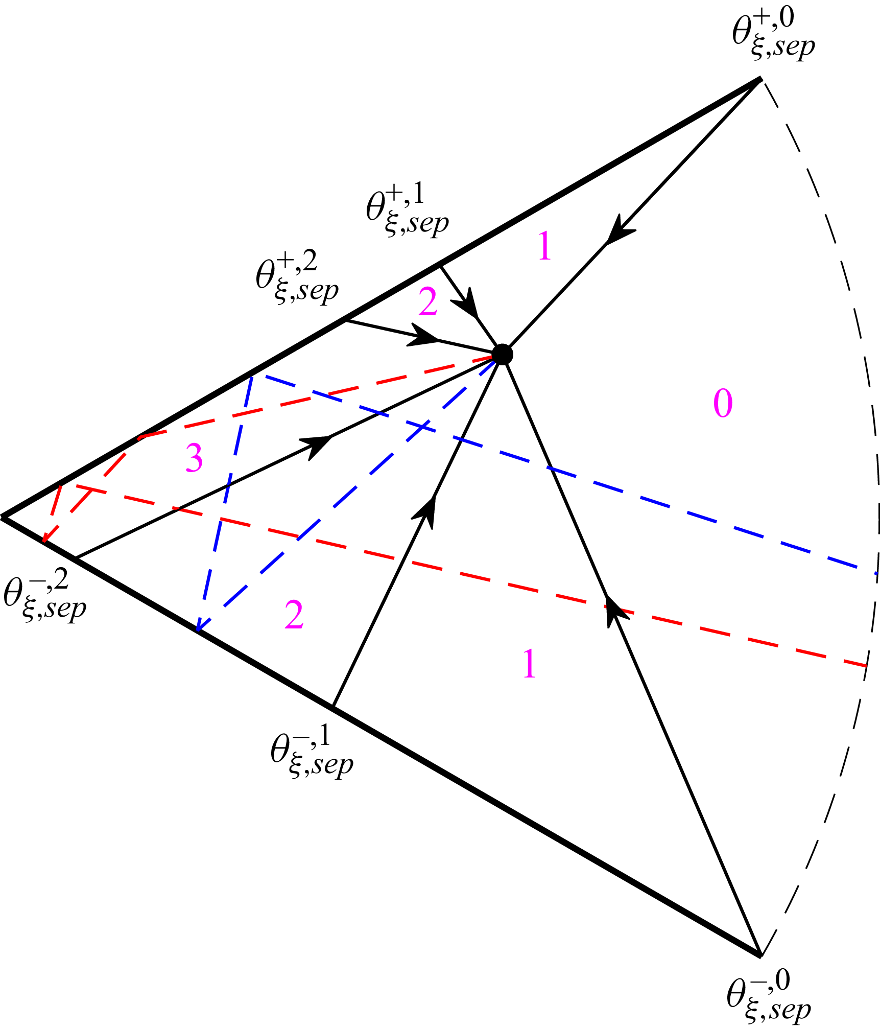


 Open access