


1. Introduction
A variety of applications in science and engineering fall within the compressible flow regime. Generally speaking, compressible flows can be categorized as pertaining to different regimes based on Mach numbers, i.e. subsonic, transonic, supersonic and hypersonic flows. Considerable advances have been achieved in numerical methods, such as shock capturing and non-oscillatory schemes (Harten Reference Harten1983; Harten et al. Reference Harten, Engquist, Osher and Chakravarthy1987; Liu, Osher & Chan Reference Liu, Osher and Chan1994), to solve the compressible Navier–Stokes–Fourier (NSF) equations along with the advent of new and more powerful computing technologies. A remaining challenge is to develop a method capable of simulating the full range of flows from subsonic to hypersonic regimes. In particular, hypersonic flows with Mach numbers greater than five can, in some cases, be quite challenging to model using classical approaches relying on the NSF equations (Tsien Reference Tsien1946; Bird Reference Bird1970). As the Knudsen number increases, the local state of the gas gets further away from the local thermodynamic equilibrium and the notion of the gas as a continuum-equilibrium fluid becomes questionable, in turn limiting the range of applicability of the NSF. For instance shock profiles for Mach numbers above two as obtained from the NSF are known not to match experimental observations and direct simulation Monte Carlo results, see for instance Greenshields & Reese (Reference Greenshields and Reese2007). The shortcomings of the NSF in these regimes have prompted the development of a variety of modified balance equations. One preferred, and rather successful approach to building balance laws beyond NSF, has been to derive reduced models based on the kinetic theory of gases, i.e. the Boltzmann equation and its variant. Over the years this has led to a variety of models, such as the more successful Grads moments method (Grad Reference Grad1949) and its many variants, see Struchtrup (Reference Struchtrup2005) for an overview. Another class of methods based on the kinetic theory of gases directly solves a discrete version of the Boltzmann equation in particle velocity space with quadratures guaranteeing correct recovery of moments of interest for the target balance equations. The now very popular lattice Boltzmann method (LBM) falls in that category.
The LBM, introduced in the early 1990s, was initially developed with the incompressible limit of the Navier–Stokes equations in mind (McNamara & Zanetti Reference McNamara and Zanetti1988; Benzi, Succi & Vergassola Reference Benzi, Succi and Vergassola1992). The past two decades have witnessed considerable efforts to extend the LBM to the compressible flow regime. These efforts can be categorized into two main approaches: (a) higher-order lattices and (b) two-population solvers with standard lattices. In the former Frapolli, Chikatamarla & Karlin (Reference Frapolli, Chikatamarla and Karlin2015), the use of a larger number of discrete velocities and higher-order quadratures allows for the recovery of higher-order moments of the distribution function, in principle, correctly recovering the energy balance equation. While these approaches were successfully used to model compressible flows the computation and communication overhead brought about by the larger stencils is rather large especially considering the limited gain in maximum achievable Mach numbers. Furthermore, it has been observed that larger stencils result in more restricted stability domains in terms of temperature. It is worth noting that a number of recent studies have proposed solutions to improve numerical properties by using higher-order Hermite roots-based lattices. This has led to the development of semi-Lagrangian high-order lattice schemes which have been used for low supersonic flows (Wilde et al. Reference Wilde, Krämer, Reith and Foysi2020). As a way to reduce computational load for extension of the models to three-dimensional (3-D) models, the authors have also proposed strategies to reduce the number of discrete velocities (Wilde et al. Reference Wilde, Krämer, Bedrunka, Reith and Foysi2021). The second category of approaches relies on the classical first-neighbour stencil supplemented with a second set of distribution functions carrying the total energy (Saadat et al. Reference Saadat, Hosseini, Dorschner and Karlin2021). This class of models has been used to simulate a variety of flows in the transonic and supersonic regimes; however, it remains restricted to low supersonic speeds. In parallel with the double distribution function approach, a number of studies have also proposed hybrid models replacing the second distribution function with discrete, finite volumes or finite differences solvers for the energy balance equation, see for instance (Feng, Sagaut & Tao Reference Feng, Sagaut and Tao2015; Renard et al. Reference Renard, Feng, Boussuge and Sagaut2021). While these approaches have been successful in modelling transonic flows and in some cases low supersonic flows, extension to higher Mach numbers has been quite challenging. A point common to all approaches is that their operation range is limited by the reference frame (Frapolli, Chikatamarla & Karlin Reference Frapolli, Chikatamarla and Karlin2016b), which is the static frame with a reference temperature dictated by the Gauss–Hermite quadrature. Other classes of solvers such as the discrete Boltzmann method (DBM), relying on the same principle as LBM for the discretization of particles speed space suffer from the same limitations, i.e. restricted operation range (see Xu et al. Reference Xu, Zhang, Gan, Chen and Yu2012; Gan et al. Reference Gan, Xu, Zhang, Zhang and Succi2018b; Ji, Lin & Luo Reference Ji, Lin and Luo2021).
In recent years, discrete velocity methods formulated on an adaptive reference frame, i.e. the particles on demand (PonD) method and its variants, have shown promising results (Frapolli et al. Reference Frapolli, Chikatamarla and Karlin2016b; Dorschner, Bösch & Karlin Reference Dorschner, Bösch and Karlin2018). By adapting the reference frame of the discrete solver to the local fluid speed and temperature, higher-order moments are kept under control and the operation range of the solver is extended to very large Mach numbers. One consequence of the change in reference frame is that the streaming operator, for a Lagrangian solver, is no longer on the lattice. To that end, most Lagrangian realizations rely on an additional interpolation step to reconstruct distribution functions on the grid. While successfully applied to a number of flow configurations, they have been observed to suffer from conservativity issues due to the interpolation step, especially in flows involving large gradients (Kallikounis, Dorschner & Karlin Reference Kallikounis, Dorschner and Karlin2022; Sawant, Dorschner & Karlin Reference Sawant, Dorschner and Karlin2022). A flux-conserving realization of the PonD following the discrete unified gas kinetic scheme (Guo, Xu & Wang Reference Guo, Xu and Wang2013) was recently introduced by Kallikounis et al. (Reference Kallikounis, Dorschner and Karlin2022). Restoration of conservative properties along with a regularized frame-to-frame transformation was shown to noticeably improve results and allow for large Mach number simulations.
Here, building upon the idea of the PonD method, different from the discrete unified gas kinetic scheme realization we propose a fully Eulerian finite-volume PonD solver for high-Mach-number flows. The outline of the paper is as follows. Section 2 presents a full procedure of model construction. The continuous kinetic equations are discretized in the phase space, which give adjustable Prandtl number and specific heat ratio. In addition, temporal and spatial discretization in an adaptive reference frame are presented and an overall algorithm is shown to clarify how to implement the new model. In § 3, a variety of simulations from simple low Mach one-dimensional (1-D) cases to more challenging 1-D and two-dimensional (2-D) configurations involving large variations in macro quantities are carried out to validate the new model. Furthermore, § 4 extends the proposed model to describe reactive flows where chemical reactions are coupled with fluid flows. Detonations are simulated with the developed model. In addition, a summary is provided in § 5.
2. Model description
In this part we will focus on model construction, starting from the Boltzmann equation with the Bhatnagar–Gross–Krook approximation for the collision operator (Bhatnagar, Gross & Krook Reference Bhatnagar, Gross and Krook1954)
 \begin{equation} \partial_t f \left (t,\boldsymbol{r}, \boldsymbol{v}\right ) + \boldsymbol{v} \boldsymbol{\cdot} \boldsymbol{\nabla} f\left (t,\boldsymbol{r} , \boldsymbol{v}\right ) = \varOmega_f, \end{equation}
where  $\varOmega _f= [\,f^{eq} (t,\boldsymbol {r} , \boldsymbol {v} )-f (t,\boldsymbol {r}, \boldsymbol {v} ) ]/ \tau$ is the collision term. $f (t,\boldsymbol {r}, \boldsymbol {v} )$ and $f^{eq} (t,\boldsymbol {r} , \boldsymbol {v} )$ represent, respectively, the distribution function and the local equilibrium distribution function. Here $\boldsymbol {v}$ designates the particle velocity and $\boldsymbol {r}$ the position in space. Here, a single parameter, $\tau$, controls the relaxation rate of the distribution function towards equilibrium state, known as local Maxwellian distribution parameterized by values of local temperature $T$, fluid velocity $\boldsymbol {u}$ and density $\rho$:
 \begin{equation} f^{eq}\left (t,\boldsymbol{r} , \boldsymbol{v}\right ) = \frac{\rho}{{(2{\rm \pi} R T)}^{D/2}} \exp\left[-\frac{{(\boldsymbol{v}-\boldsymbol{u})}^2}{2RT}\right], \end{equation}
where  $D$ is the dimension of the physical space and $R$ designates the gas constant. For the sake of convenience, $R=1$ is used in the rest of this paper.
To take into account the effect of internal degrees of freedom allowing for variable specific heat ratios  $\gamma$, following Rykov's original work (Rykov Reference Rykov1976) we supplement (2.1) with a balance equation for a second distribution function $g$ carrying the excess internal energy stemming from non-translational degrees of freedom:
 \begin{equation} \partial_t g \left (t,\boldsymbol{r}, \boldsymbol{v} \right ) + \boldsymbol{v} \boldsymbol{\cdot}\boldsymbol{\nabla} g\left (t,\boldsymbol{r} , \boldsymbol{v}\right ) = \varOmega_g, \end{equation}
with  $\varOmega _g= (g^{eq} (t,\boldsymbol {r}, \boldsymbol {v} ) - g (t,\boldsymbol {r}, \boldsymbol {v} ) )/ \tau$. Following the definition of the second distribution function, the local equilibrium state $g^{eq}$ can be defined as
 \begin{equation} g^{eq} = 2\left (C_v-\frac{D}{2}\right )T f^{eq}, \end{equation}
where  $C_v$ indicates the specific heat at constant volume. As a result the total energy can be obtained as
 \begin{equation} \rho E = \rho (C_v T +\tfrac{1}{2} | \boldsymbol{u} |^2)= \int \tfrac{1}{2} \,f | \boldsymbol{v} |^2 \,{\rm d}\boldsymbol{v} + \int \tfrac{1}{2} g \,{\rm d}\boldsymbol{v}. \end{equation}
While allowing for variable specific heat ratios, given that all moments relax at the same rate, the model still is limited to unity Prandtl number, defined as
 \begin{equation} Pr = \frac{{C}_p \mu}{\kappa}, \end{equation}
where  $C_p$ is specific heat under constant pressure, $\mu$ the dynamic viscosity and $\kappa$ the thermal conductivity.
To overcome this restriction, the relaxation to the equilibrium is split into two steps via the introduction of an intermediary state called the quasiequilibrium state (Gorban & Karlin Reference Gorban and Karlin1994; Ansumali et al. Reference Ansumali, Arcidiacono, Chikatamarla, Prasianakis, Gorban and Karlin2007; Frapolli, Chikatamarla & Karlin Reference Frapolli, Chikatamarla and Karlin2014, Reference Frapolli, Chikatamarla and Karlin2016a; Hosseini & Karlin Reference Hosseini and Karlin2023). The collision terms are rewritten as
 $$\begin{gather} \varOmega_f= \frac{1}{\tau_1} \left [\,f^{eq}\left (t,\boldsymbol{r} , \boldsymbol{v}\right )-f\left (t,\boldsymbol{r} , \boldsymbol{v}\right ) \right ] + \left ( \frac{1}{\tau_1} -\frac{1}{\tau_2} \right ) \left [\,f^{*}\left (t,\boldsymbol{r}, \boldsymbol{v} \right ) - f^{ eq}\left (t,\boldsymbol{r} , \boldsymbol{v}\right ) \right ], \end{gather}$$
 $$\begin{gather}\varOmega_g= \frac{1}{\tau_1} \left [g^{eq}\left (t,\boldsymbol{r}, \boldsymbol{v} \right )-g\left (t,\boldsymbol{r}, \boldsymbol{v} \right ) \right ] + \left ( \frac{1}{\tau_1} -\frac{1}{\tau_2} \right ) \left [ g^{*}\left (t,\boldsymbol{r}, \boldsymbol{v} \right ) - g^{ eq}\left (t,\boldsymbol{r} , \boldsymbol{v}\right ) \right ], \end{gather}$$
where  $\tau _1$ and $\tau _2$ are the two relaxation parameters related to the viscosity and thermal conductivity, and $f^{*} (t,\boldsymbol {r}, \boldsymbol {v} )$ and $g^{*} (t,\boldsymbol {r}, \boldsymbol {v} )$ are quasiequilibria.
In fact, the quasiequilibrium state is defined as the minimizer of the Boltzmann entropy function subject to a set of locally conserved fields and quasiconserved slow fields. Following Ansumali et al. (Reference Ansumali, Arcidiacono, Chikatamarla, Prasianakis, Gorban and Karlin2007), in order to recover the NSF equations with variable Prandtl number, the quasiequilibrium distribution functions are required to satisfy the conservation of mass, momentum and total energy,
 $$\begin{gather} \int \left \{ 1,v_{\alpha} \right \} f^{*} \,{\rm d}\boldsymbol{v}= \int \left \{ 1, v_{\alpha} \right \} f^{eq} \,{\rm d}\boldsymbol{v}, \end{gather}$$
 $$\begin{gather}\int \left(| \boldsymbol{v} |^ 2 f^{*} +g^{*}\right) {\rm d}\boldsymbol{v} = \int \left(| \boldsymbol{v} |^2 f^{eq} + g^{eq}\right) {\rm d}\boldsymbol{v}. \end{gather}$$
In addition, the quasiequilibrium distribution functions are designed to conserve the third-order centred kinetic moments defined as
 $$\begin{gather} \bar{Q}_{\alpha \beta \gamma} = \int f \left (v_{\alpha}- u_{\alpha}\right)\left (v_{\beta}- u_{\beta}\right)\left (v_{\gamma}- u_{\gamma}\right){\rm d}\boldsymbol{v}, \end{gather}$$
 $$\begin{gather}\bar{q}_{\alpha} = \int \left(\,f | \boldsymbol{v} -\boldsymbol{u}|^2 +g \right)\left (v_{\alpha}- u_{\alpha}\right) {\rm d}\boldsymbol{v} , \end{gather}$$
where  $\bar {Q}_{\alpha \beta \gamma }$ is the centred heat flux tensor and $\bar {q}_{\alpha }$ the centred heat flux. The constraints for the two quasiconserved quantities are
 $$\begin{gather} \bar{Q}_{\alpha \beta \gamma}^{*} = \bar{Q}_{\alpha \beta \gamma}, \end{gather}$$
 $$\begin{gather}\bar{q}_{\alpha}^{*} = \bar{q}_{\alpha}. \end{gather}$$
Here,  $\bar {Q}_{\alpha \beta \gamma }^{*}$ and $\bar {q}_{\alpha }^{*}$ are constructed by substituting $f$ with $f^*$ in (2.11) and (2.12), respectively. These two constraints are the keys to realize an adjustable Prandtl number. In this way, Prandtl number ${Pr}$ can be controlled by adjusting $\tau _1$ and $\tau _2$ independently as
 \begin{equation} {Pr} = \frac{\tau_1}{\tau_2}. \end{equation}
Using the new collision terms (2.7) and (2.8), the kinetic equations (2.1) and (2.3) are partial differential equations (PDEs) in time, physical space and phase space – the space of the particles’ velocities. In the upcoming sections we will introduce methods to discretize these equations while retaining conservativity and capturing the hydrodynamic regime, Euler and NSF, even under extreme conditions, i.e. large Mach number and temperature variations.
2.1. Discretization in phase space
2.1.1. Frame-invariance of the Boltzmann equation
Before moving on into the details of the proposed discrete solver a brief discussion on the concept of frame is in order. A frame  $\lambda (\boldsymbol {u}^\lambda,T^\lambda )$, as intended here, is parameterized by a reference velocity, $\boldsymbol {u}^\lambda$, and a reference temperature, $T^\lambda$. Particle velocities can therefore be written under this transformation of phase-space as
 \begin{equation} \boldsymbol{v}^{\lambda(\boldsymbol{u}^\lambda,T^\lambda)} = \frac{\boldsymbol{v} - \boldsymbol{u}^\lambda}{\sqrt{T^\lambda}}. \end{equation}
It is straightforward to show, simply through the invariance of the corresponding moments system, the equivalence of Boltzmann equations on different frames, i.e.
 \begin{equation} D_t^\lambda \{\,f^{\lambda}, g^{\lambda}\} \left (t,\boldsymbol{r},\boldsymbol{v}^{\lambda} \right ) = \varOmega_{\{\,f^{\lambda}, g^{\lambda}\}} \Leftrightarrow D_t^{\lambda'} \{\,f^{\lambda'}, g^{\lambda'}\} \left (t,\boldsymbol{r},\boldsymbol{v}^{\lambda'} \right ) = \varOmega_{\{\,f^{\lambda'}, g^{\lambda'}\}}, \end{equation}
where we have used the short-hand notation  $D_t^\lambda = \partial _t + \boldsymbol {v}^\lambda \boldsymbol{\cdot}\boldsymbol {\nabla }$. Note that for the equivalence to stand, in each system the reference frame is fixed.
2.1.2. Frame-invariance of discrete velocity Boltzmann equations
Discretization of the particles’ velocity space is usually achieved through finite-order quadratures, such as the Gauss–Hermite quadrature (Shan & He Reference Shan and He1998), guaranteeing that moments of the continuous distribution function are matched by the discrete distribution function up to the order of the quadrature. Defining moments of the discrete distribution functions as
 \begin{equation} M_{\underbrace{x\dots x}_{p_x},\underbrace{y\dots y}_{p_y},\underbrace{z\dots z}_{p_z}}(\boldsymbol{c}_i, \{\,f_i^\lambda, g_i^\lambda\}) = \sum_{i=1}^{Q} \overbrace{\prod_{\alpha=x,y,z} {\left(\sqrt{T^\lambda}c_{i\alpha} + u_{\alpha}^\lambda\right)}^{p_\alpha}}^{\phi^\lambda(\boldsymbol{c}_i)} \{\,f_i^\lambda, g_i^\lambda\}, \end{equation}
we can introduce the set  $\varPhi$ of functions $\phi$ such that
 \begin{equation} \sum_{i=1}^{Q} \phi^\lambda(\boldsymbol{c}_i) \{\,f_i^\lambda, g_i^\lambda\} = \int_{} \phi^\lambda(\boldsymbol{v}^\lambda) \{\,f^\lambda, g^\lambda\} \,{\rm d}\boldsymbol{v}, \end{equation}
to define the set of moments supported by the lattice quadrature. Using (2.19) and the discussion in the previous section on frame-invariance of moments of the continuous distribution functions we can readily establish the frame-invariance of the set of moments defined by  $\varPhi$ of the discrete distribution functions. Moving one step forward one can also readily demonstrate the frame-invariance of the moments balance equations:
 \begin{align} &\partial_t \sum_{i=1}^{Q} \phi'^\lambda\{\,f_i^{\lambda}, g_i^{\lambda}\} + \boldsymbol{\nabla}\boldsymbol{\cdot}\left(\sqrt{T^\lambda}\boldsymbol{c}_i + \boldsymbol{u}^\lambda\right) \phi'^\lambda\{\,f_i^{\lambda}, g_i^{\lambda}\} = \sum_{i=1}^{Q} \phi'^\lambda \varOmega_{\{\,f_i^{\lambda}, g_i^{\lambda}\}} \nonumber\\ &\quad \Leftrightarrow \partial_t \sum_{i=1}^{Q} \phi'^{\lambda'}\{\,f_i^{\lambda'}, g_i^{\lambda'}\} + \boldsymbol{\nabla}\boldsymbol{\cdot}\left(\sqrt{T^{\lambda'}}\boldsymbol{c}_i + \boldsymbol{u}^{\lambda'}\right) \phi'^{\lambda'}\{\,f_i^{\lambda'}, g_i^{\lambda'}\} = \sum_{i=1}^{Q} \phi'^{\lambda'} \varOmega_{\{\,f_i^{\lambda'}, g_i^{\lambda'}\}}, \end{align}
where  $\phi '^\lambda$ defines the set of moments such that $(\sqrt {T^\lambda }\boldsymbol {c}_i + \boldsymbol {u}^\lambda )\varPhi '^\lambda \in \varPhi$. For higher-order moments the equivalence is lost due to the limited order of the quadrature. Using these moments equations and further a multiscale analysis, see Kallikounis & Karlin (Reference Kallikounis and Karlin2024) for details, one can establish the order of quadrature needed to correctly recover the target balance equations.
2.1.3. Particles on demand
To eliminate errors in higher-order moments of the distribution function not supported by the lattice quadrature, in the PonD method (Dorschner et al. Reference Dorschner, Bösch and Karlin2018), the reference frame is chosen via the local macroscopic quantities, i.e. fluid speed and temperature
 \begin{equation} T^{\lambda} = T, \quad \boldsymbol{u}^\lambda = \boldsymbol{u}. \end{equation}
In doing so equilibrium distribution functions are accurately evaluated and only depend on the local density
 \begin{equation} f_i^{eq} = \rho W_i, \end{equation}
where  $W_i$ are weights of the Gauss–Hermite quadrature (Frapolli et al. Reference Frapolli, Chikatamarla and Karlin2015). Based on this, the discrete quasiequilibrium distribution functions under constraints (2.9)–(2.10) and (2.13)–(2.14) have the following expression for $Pr < 1$:
 $$\begin{gather} f_i^{*} = f_i^{eq} + W_i \boldsymbol{\bar{Q}} : \left( \boldsymbol{v}_i \otimes \boldsymbol{v}_i \otimes \boldsymbol{v}_i - 3T \boldsymbol{v}_i \boldsymbol{I} \right)/6T^3, \end{gather}$$
 $$\begin{gather}g_i^{*} = g_i^{eq} + W_i \boldsymbol{\bar{q}} \boldsymbol{\cdot} \boldsymbol{v}_i /T, \end{gather}$$
where  $\boldsymbol {I}$ is the unit tensor, ‘:’ is the Frobenius inner tensorial product and $\otimes$ denotes tensor product. The choice of the reference frame based on local velocity and temperature would, at first sight, lead to a space- and time-dependent reference frame.
Different from approaches such as Kauf (Reference Kauf2011) and Köllermeier (Reference Köllermeier2013) where an adaptive reference-based Boltzmann equation is solved globally in the domain bringing in non-commutativity of the discrete velocities with the space- and time-derivatives and resulting in additional terms in the Boltzmann equation involving derivatives of the reference frame velocity and temperature, in PonD at every point in space and time,  $\boldsymbol {r}$ and $t$, the Boltzmann equation is solved in the fixed reference frame of that point, here denoted as $\bar {\lambda }$ for the sake of readability,
 \begin{equation} D_t^{\bar{\lambda}} \mathcal{M}_{\lambda(\boldsymbol{r},t)}^{\bar{\lambda}}\{\,f_i^{\lambda(\boldsymbol{r},t)}, g_i^{\lambda(\boldsymbol{r},t)}\} = \mathcal{M}_{\lambda(\boldsymbol{r},t)}^{\bar{\lambda}} \varOmega_{\{\,f_i^{\lambda(\boldsymbol{r},t)}, g_i^{\lambda(\boldsymbol{r},t)}\}}, \end{equation}
where  $\mathcal {M}_{\lambda (\boldsymbol {r},t)}^{\bar {\lambda }}$ is the reference frame transformation operator discussed in the next section.
2.1.4. Distribution function transformation: Grad's projection
Given the invariance of moments supported by the lattice quadrature, a straightforward approach to the transformation of distribution functions between different reference frames  $\lambda = ( \boldsymbol {u}^{\lambda }, T^{\lambda } )$ and $\lambda ' = ( \boldsymbol {u}^{\lambda '}, T^{\lambda '} )$ would be to match moments,
 \begin{equation} \boldsymbol{M}^{\lambda} = \boldsymbol{M}^{\lambda '}. \end{equation}
Another approach, proposed in Zipunova et al. (Reference Zipunova, Perepelkina, Zakirov and Khilkov2021) and further extended in Kallikounis et al. (Reference Kallikounis, Dorschner and Karlin2022) is the regularized reconstruction of distribution functions. In the regularized approach the distribution function in the new reference frame  $\lambda '$ is sought in the form of a finite-order Grad expansion,
 \begin{equation} f_i^{\lambda'} = W_i \sum_{n=0}^{N} \frac{1}{n! T_L^n} \boldsymbol{a}^{\lambda'}_{\left(n \right)} : \boldsymbol{H}_i^{\left(n \right)} \left( \boldsymbol{c}_i \right)\!, \end{equation}
where  $\boldsymbol {a}^{\lambda '}_{(n )}$ and $\boldsymbol {H}_i^{(n )} ( \boldsymbol {c}_i )$ are tensors of rank $n$ denoting the Hermite coefficient and polynomial of the corresponding order in the $\lambda '$ reference frame, $N$ is the order of the Grad expansion and $T_L$ the lattice temperature. Solving (2.26) one can derive the Grad coefficients in the reference frame $\lambda '$ as a function of moment in $\lambda$; for instance, for the first three coefficients,
 $$\begin{gather} a_0^{\lambda'} = M^\lambda_0, \end{gather}$$
 $$\begin{gather}a_1^{\lambda'} = \frac{1}{\sqrt{T^{\lambda'}/T_L}}\left(M^\lambda_1 - M_0^\lambda u^{\lambda'}\right)\!, \end{gather}$$
 $$\begin{gather}a_{2}^{\lambda'} = \frac{T_L}{T^{\lambda'}}\left(M^\lambda_2 - M_0^\lambda T^{\lambda'} \boldsymbol{I} - \sqrt{T^{\lambda'}/T_L}\overline{u^{\lambda'}\otimes a_1^{\lambda'}} - M_0^\lambda u^{\lambda'}\otimes u^{\lambda'}\right) \end{gather}$$
and
 \begin{align} a_{3}^{\lambda'} &= \frac{1}{{\left(T^{\lambda'}/T_L\right)}^{3/2}}\left(M^\lambda_3 - \frac{T^{\lambda'}}{T_L} \overline{u^{\lambda'}\otimes\left(M_0^\lambda T_L\boldsymbol{I} + a_2^{\lambda'}\right)} - T^{\lambda'}\sqrt{\frac{T^{\lambda'}}{T_L}} \overline{a_1^{\lambda'}\otimes \boldsymbol{I}} \right. \nonumber\\ &\quad \left. - \sqrt{\frac{T^{\lambda'}}{T_L}} \overline{a_1^{\lambda'}\otimes u^{\lambda'} \otimes u^{\lambda'}} - M_0^{\lambda} u^{\lambda'} \otimes u^{\lambda'} \otimes u^{\lambda'}\right). \end{align}
 Equations (2.26) to (2.31) allow us to go transform distribution function from reference frame  $\lambda$ to $\lambda '$:
 \begin{equation} f_i^{\lambda} = \mathcal{M}_{\lambda '}^{\lambda} f_i^{\lambda '} , \end{equation}
where  $\mathcal {M}_{\lambda '}^{\lambda }$ is a short notation for transformation operation. To capture fundamental flow physics properties at the NSF level, up to third-order expansion is necessary for $f_i$, while for the internal distribution function $g_i$, the second-order expansion is sufficient. Furthermore, we use a fourth-order quadrature for the discrete velocities in this study, i.e. the D2Q16 model in 2-D (Ansumali, Karlin & Öttinger Reference Ansumali, Karlin and Öttinger2003; Kallikounis & Karlin Reference Kallikounis and Karlin2024). The necessary characteristics of the D2Q16 lattice are listed in table 1 and the Hermite coefficients are provided in Appendix B.
Lattice temperature  $T_L$, roots of Hermite polynomials $c_{i \alpha }$ and weights $W_{i \alpha }$ for D2Q16.

2.2. Time- and space-discretization: finite volume realization
2.2.1. Finite volume formulation
Different from the commonly used ‘ $\text {propagation}+\text {collision}$’ scheme in most LB solvers, the present work we make use of a fully Eulerian finite volume discretization, therefore targeting the integral form of the local discrete Boltzmann PDE system of (2.25) in the reference frame $\bar {\lambda }$:
 \begin{align} &\partial_t^{\bar{\lambda}} \int_{\delta V} \mathcal{M}_{\lambda(\boldsymbol{r},t)}^{\bar{\lambda}}\{\,f_i^{\lambda(\boldsymbol{r},t)}, g_i^{\lambda(\boldsymbol{r},t)}\} \,{\rm d}\boldsymbol{r} + \int_{\delta S} \boldsymbol{n} \boldsymbol{\cdot} \boldsymbol{v}_i^{\bar{\lambda}} \mathcal{M}_{\lambda(\boldsymbol{r},t)}^{\bar{\lambda}}\{\,f_i^{\lambda(\boldsymbol{r},t)}, g_i^{\lambda(\boldsymbol{r},t)}\} \,{\rm d}S\nonumber\\ &\quad = \int_{\delta V}\mathcal{M}_{\lambda(\boldsymbol{r},t)}^{\bar{\lambda}} \varOmega_{\{\,f_i^{\lambda(\boldsymbol{r},t)}, g_i^{\lambda(\boldsymbol{r},t)}\}}\,{\rm d}\boldsymbol{r}, \end{align}
where  $\boldsymbol {n}$ is the outwards unit vector normal to the surface $S$ and $\delta V$ is an infinitesimal control volume defining the grid and $\delta S$ the corresponding surface. For a given unit volume bound by discrete surfaces $\sigma$ one obtains the space-discretized system of equations as
 \begin{equation} \delta V \partial_t \{\,f_i^{\bar{\lambda}}, g_i^{\bar{\lambda}}\} + \sum_{\sigma \in S} \{\mathcal{F}_i^{\bar{\lambda}}, \mathcal{G}_i^{\bar{\lambda}}\}\left(\sigma\right) = \int_{\delta V} \varOmega_{\{{\,f_i}^{\bar{\lambda}}, {g_i}^{\bar{\lambda}}\}} \,{\rm d}\boldsymbol{r}, \end{equation}
where  $\{\mathcal {F}_i^{\bar {\lambda }}, \mathcal {G}_i^{\bar {\lambda }}\}(\sigma )$ are the fluxes at interfaces $\sigma$ surrounding the control volume and making up $\delta S$. The cell-averaged distribution functions appearing here are defined as
 \begin{equation} \{\,f_i^{\bar{\lambda}}, g_i^{\bar{\lambda}}\} = \frac{1}{\delta V}\int_{\delta V} \mathcal{M}_{\lambda(\boldsymbol{r},t)}^{\bar{\lambda}}\{\,f_i^{\lambda(\boldsymbol{r},t)}, g_i^{\lambda(\boldsymbol{r},t)}\} \,{\rm d}\boldsymbol{r}. \end{equation}
As a result, the local macroscopic properties obtained as moments of the distribution function, are also cell-averaged values, i.e.
 $$\begin{gather} \bar{\rho} = \sum_{i=1}^Q \bar{f}_i^{\bar{\lambda}}, \end{gather}$$
 $$\begin{gather}\bar{\rho \boldsymbol{u}} = \sum_{i=1}^Q \boldsymbol{v}_i^{\bar{\lambda}}\bar{f}_i^{\bar{\lambda}} \end{gather}$$
and
 \begin{equation} \bar{E} = \sum_{i=1}^Q | \boldsymbol{v}_i^{\bar{\lambda}} |^2 \bar{f}_i^{\bar{\lambda}} + \sum_{i=1}^Q \bar{g}_i^{\bar{\lambda}}. \end{equation}
2.2.2. Time discretization: first-order Euler
While the time derivative term can be discretized using any of the available higher-order approaches, e.g. Runge–Kutta schemes, etc., here for the sake of simplicity, time stepping is carried out using a fully explicit first-order Euler scheme,
 \begin{equation} \partial_t \{\,f_i^{\bar{\lambda}}, g_i^{\bar{\lambda}}\} = \frac{\{\,f_i^{\bar{\lambda}}, g_i^{\bar{\lambda}}\}\left(t+\delta t\right) - \{\,f_i^{\bar{\lambda}}, g_i^{\bar{\lambda}}\}\left(t\right)}{\delta t} + O(\delta t), \end{equation}
resulting in the following discrete equations:
 \begin{align} \{\,f_i^{\bar{\lambda}}, g_i^{\bar{\lambda}}\}\left(t+\delta t,\boldsymbol{r}\right) &= \{\,f_i^{\bar{\lambda}}, g_i^{\bar{\lambda}}\}\left(t,\boldsymbol{r}\right) - \frac{\delta t}{\delta V}\sum_{\sigma \in S} \{\mathcal{F}_i^{\bar{\lambda}}, \mathcal{G}_i^{\bar{\lambda}}\} \left(t,\sigma\right) \nonumber\\ &\quad + \frac{\delta t}{\delta V} \int_{\delta V} \varOmega_{\{{\,f_i}^{\bar{\lambda}}, {g_i}^{\bar{\lambda}}\}}\left(t,\boldsymbol{r}\right) {\rm d}\boldsymbol{r}. \end{align}
2.2.3. Collision operator
In the context of the present first order in-time realization the collision term is evaluated explicitly and on the cell-averaged reference frame of the control volume, i.e.  $\bar {\lambda }$:
 \begin{equation} \frac{\delta t}{\delta V} \int_{\delta V} \varOmega_{{f_i}^{\bar{\lambda}}}\left(t,\boldsymbol{r}\right) {\rm d}\boldsymbol{r} = \frac{\delta t}{\tau_1}\left[\bar{\rho} W_i - \bar{f}_i^{\bar{\lambda}}\right] + \left(\frac{\delta t}{\tau_1} - \frac{\delta t}{\tau_2}\right) \left[\bar{f^*}^{\bar{\lambda}}_i - \bar{\rho} W_i\right] \end{equation}
and
 \begin{align} \frac{\delta t}{\delta V} \int_{\delta V} \varOmega_{{g_i}^{\bar{\lambda}}}\left(t,\boldsymbol{r}\right) {\rm d}\boldsymbol{r} &= \frac{\delta t}{\tau_1}\left[2\bar{\rho}\bar{T}\left(C_v-\frac{D}{2}\right) W_i - \bar{g}_i^{\bar{\lambda}}\right]\nonumber\\ &\quad + \left(\frac{\delta t}{\tau_1} - \frac{\delta t}{\tau_2}\right) \left[\bar{g^*}^{\bar{\lambda}}_i - 2\bar{\rho}\bar{T}\left(C_v-\frac{D}{2}\right) W_i\right]\!. \end{align}
Note that though not the main focus of the present contribution, the Crank–Nicolson second-order approximation akin to the redefined fluxes in the LBM can also be implemented with the present FVM realization.
2.2.4. Streaming operator: flux reconstruction
Next comes the issue of reconstruction of fluxes at interfaces, and with it two challenges: one that is common to all PDEs i.e. reconstruction of fluxes at interfaces from volume-averaged fields and one specific to the present model, the choice of the reference frame  $\tilde {\lambda }$ in which fluxes are to be reconstructed.
To have exact conservation at cell interfaces, out-flux from a given cell must match exactly the in-flux from its neighbour, which is only guaranteed by setting  $\tilde {\lambda }$ to that of their interface. For the first issue, as for any other PDE, pointwise values at cell interfaces are computed on the basis of a pointwise field reconstructed through polynomial interpolation from the corresponding cell-averaged field. This is illustrated for the case of a 1-D system in figure 1. There, $\mathcal {F} (t, {x-{\delta x}/{2}})$ and $\mathcal {F} (t, {x+{\delta x}/{2}})$ are the left- and right-hand interface fluxes at $x-{\delta x}/{2}$ and $x+{\delta x}/{2}$, respectively. Assuming a linear shape function and using a centred scheme,
 \begin{equation} \mathcal{F}_i^{\lambda(t, {x-{\delta x}/{2}})} \left(t, x-\frac{\delta x}{2}\right) =-v_i^{\lambda(t,x-{\delta x}/{2})} \left(t, {x-\frac{\delta x}{2}}\right) f_i^{\lambda(t, {x-{\delta x}/{2}})} \left(t, x-\frac{\delta x}{2}\right)\!, \end{equation}
with
 \begin{equation} v_i^{\lambda(t,x-{\delta x}/{2})} \left(t, {x-\frac{\delta x}{2}}\right) = \frac{v_i^{\lambda(t,x-\delta x)} \left(t, {x-\delta x}\right) + v_i^{\lambda(t,x)} \left(t, {x}\right)}{2} \end{equation}
and
 \begin{equation} f_i^{\lambda(t, {x-{\delta x}/{2}})} \left(t, x-\frac{\delta x}{2}\right) = \frac{f_i^{\lambda(t, {x-{\delta x}/{2}})} \left(t, x-\delta x\right) + f_i^{\lambda(t, {x-{\delta x}/{2}})} \left(t, x\right)}{2}. \end{equation}
For the first-order upwind scheme, here the left-hand interface flux  $\mathcal {F}_i^{\lambda (t, {x-{\delta x}/{2}})} (t, x-{\delta x}/{2})$ uses the similar recipe as
 \begin{equation} \mathcal{F}_i^{\lambda(t, {x-{\delta x}/{2}})} \left(t, x-\frac{\delta x}{2}\right) =-v_i^{\lambda(t,x-{\delta x}/{2})} \left(t, {x-\frac{\delta x}{2}}\right) f_i^{\lambda(t, {x-{\delta x}/{2}})} \left(t, x-\frac{\delta x}{2}\right)\!, \end{equation}
with
 \begin{equation} f_i^{\lambda(t, {x-{\delta x}/{2}})} \left(t, x-\frac{\delta x}{2}\right) = \left \{ \begin{array}{@{}ll} {f_i^{\lambda(t, {x-{\delta x}/{2}})} \left(t, x-\delta x\right)}, & {v_i^{\lambda(t,x-{\delta x}/{2})} \left(t, {x-\dfrac{\delta x}{2}}\right) \geq 0 }\\[10pt] {f_i^{\lambda(t, {x-{\delta x}/{2}})} \left(t, x\right)}, & { v_i^{\lambda(t,x-{\delta x}/{2})} \left(t, {x-\dfrac{\delta x}{2}}\right) < 0 } \end{array}\right. \end{equation}
and
 \begin{equation} v_i^{\lambda(t, {x-{\delta x}/{2}})} \left(t, x-\frac{\delta x}{2}\right) = \left \{ \begin{array}{@{}ll} {v_i^{\lambda(t, {x-\delta x})} \left(t, x-\delta x\right)}, & { v_i^{\lambda(t, {x-\delta x})} \left(t, x-\delta x\right) \geq 0 }\\ {v_i^{\lambda(t, {x})} \left(t, x\right)}, & { v_i^{\lambda(t, {x-\delta x})} \left(t, x-\delta x\right) < 0 } \end{array}\right. . \end{equation}
Once the fluxes are computed at the interface reference frame, they can be put back into (2.40) using
 \begin{equation} \mathcal{F}_i^{\bar{\lambda}} = \mathcal{M}_{\tilde{\lambda}}^{\bar{\lambda}} \mathcal{F}_i^{\tilde{\lambda}}. \end{equation}
In order to obtain a good compromise between numerical dissipation and accuracy, a monotonic upstream-centred scheme for conservation laws (MUSCL) is adopted in the following simulations with contact discontinuity. The flux and the interface reference frame are constructed by a combination of first-order upwind scheme (low order) and second-order central scheme (high order) with a limiter function  $\phi$,
 $$\begin{gather} \mathcal{F}_i = \mathcal{F}_i^{low} -\phi(x) \left( \mathcal{F}_i^{low} - \mathcal{F}_i^{high} \right)\!, \end{gather}$$
 $$\begin{gather}v_i = v_i^{low} -\phi(x) \left( v_i^{low} - v_i^{high} \right) \end{gather}$$
and the minmod limiter is used as the limiter function (Roe Reference Roe1986)
 \begin{equation} \phi(x) = \max\left[0,\min\left( 1,x \right) \right], \end{equation}
where  $x$ represents the ratio of successive gradients.
Schematics for flux construction.

2.2.5. Flux conservation properties
As discussed in the introduction, one motivation for the development of the present realization is to overcome conservation issues encountered with semi-Lagrangian schemes. To illustrate conservation properties of the present model, we consider a cell centred at  $x$ in a 1-D system and the interface with its left-neighbouring cell centred at $x-\delta x$, located at $x-\delta x/2$. For the system to be conservative, the change in the cell-averaged value of a given moment $\bar {M}_i^{\lambda (x)}(x)$ due to left-hand flux, represented by $\delta \bar {M}_i^{\lambda (x)}(x)$,
 \begin{equation} \delta \bar{M}_i^{\lambda(x)}(x) = \delta t\sum_{i=1}^Q \mathcal{M}_{\lambda(x-\delta x/2)}^{\bar{\lambda}(x)} \{\mathcal{F}_i^{\lambda(x-\delta x/2)}, \mathcal{G}_i^{\lambda(x-\delta x/2)}\}, \end{equation}
must match the change in cell-averaged value of its left neighbour,  $\bar {M}_i^{\lambda (x-\delta x)}(x-\delta x)$, due to this same flux, $\delta \bar {M}_i^{\lambda (x-\delta x)}(x-\delta x)$,
 \begin{equation} \delta \bar{M}_i^{\bar{\lambda}(x-\delta x)}(x-\delta x) =-\delta t\sum_{i=1}^Q \mathcal{M}_{\lambda(x-\delta x/2)}^{\bar{\lambda}(x-\delta x)} \{\mathcal{F}_i^{\lambda(x-\delta x/2)}, \mathcal{G}_i^{\lambda(x-\delta x/2)}\}, \end{equation}
which translates into
 \begin{equation} \sum_{i=1}^Q \mathcal{M}_{\lambda(x-\delta x/2)}^{\bar{\lambda}(x)} \{\mathcal{F}_i^{\lambda(x-\delta x/2)}, \mathcal{G}_i^{\lambda(x-\delta x/2)}\} = \sum_{i=1}^Q \mathcal{M}_{\lambda(x-\delta x/2)}^{\bar{\lambda}(x-\delta x)} \{\mathcal{F}_i^{\lambda(x-\delta x/2)}, \mathcal{G}_i^{\lambda(x-\delta x/2)}\}, \end{equation}
meaning invariance with respect to the reference frame transformation operator is the necessary and sufficient condition for exact conservation. Following the discussion on invariance of the discrete Boltzmann equation in § 2.1.2 this means that as long as the flux of a given moment is supported by the quadrature of the lattice, conservation is ensured. To illustrate, consider the case of the invariants of the collision operator, i.e. mass, momentum and energy. To ensure conservation, the lattice must support moments  $M_0(\,f_i)$, $M_\alpha (\,f_i)$, $M_{\alpha \beta }(\,f_i)$, $M_{\alpha \alpha \beta }(\,f_i)$, $M_0(g_i)$ and $M_\alpha (g_i)$.
2.3. Overall algorithm
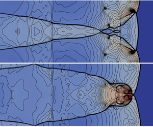
We summarize this part with a flow chart in figure 2. The evolution scheme of the present model with the finite volume formulation is implemented as
(i) compute the interfacial reference frame $\tilde {\lambda }$ by (2.44);
(ii) transform the distribution functions in the stencil from the corresponding cell-averaged frames to the interfacial frame
$\tilde {\lambda }$;(iii) calculate the interfacial distribution function
$f_i^{\tilde {\lambda }}(t)$;(iv) calculate the interfacial flux
$\mathcal {F}_i^{\tilde {\lambda }}(t)$ by (2.43);(v) obtain the flux
$\mathcal {F}_i^{\bar {\lambda }}(t)$ evaluated on the reference frame $\bar {\lambda }$ from $\mathcal {F}_i^{\tilde {\lambda }}(t)$ by (2.49);(vi) update the distribution functions through (2.40) and compute the comoving reference frame
$\bar {\lambda }$ at each cell.


Flow chart for the proposed model: red lines represent transformation between different reference frames, blue lines stand for interpolation for interfacial values and black lines indicate other operations.

3. Results and discussion
In this section, the model is validated through several 1-D and 2-D benchmarks, probing model properties such as conservation, Galilean invariance of dissipation rates, showcasing its suitability for extreme conditions involving large Mach numbers and temperature variations. For the remainder of this section, unless otherwise indicated, the specific heat ratio is  $\gamma = 1.4$, and the Prandtl number is $Pr=1$ due to the reason that these benchmarks are Euler-level problems where $Pr$ is irrelevant. The Courant–Friedrichs–Lewy (CFL) number is set as ${\rm CFL}= {\max } | \boldsymbol {u} | (\delta t/ \delta r ) = 0.2$.
3.1. Numerical properties: conservation of mass
To illustrate the necessity of adopting a flux-conserving space-discretization scheme for the present discrete velocity Boltzmann solver we first consider the simple 1-D case of the Sod shock tube with initial conditions
 \begin{equation} \left( \rho, p,u_x \right) = \left \{ \begin{array}{@{}ll} \left( 0.5,4,0 \right)\!, & 0 \leq x \leq 0.5, \\ \left( 0.5,0.5,0 \right)\!, & 0.5 < x \leq 1.0. \end{array}\right. \end{equation}
The configuration is studied both with the finite-volume realization introduced here and the original interpolation-based semi-Lagrangian PonD model Dorschner et al. (Reference Dorschner, Bösch and Karlin2018). The resolution of the computational domain in both simulations is  $L_x=500\delta x$. Figure 3 shows the evolution of total mass in the system over time for the two schemes. The total mass for the semi-Lagrangian solver is not conserved, leading in turn to incorrect density levels as shown in figure 4. Instead, the finite volume scheme makes the total mass conserved and restores correct density profiles, in agreement with the reference solution.
Comparison of temporal history of the total mass with the finite volume (solid line) and the semi-Lagrangian (symbols) schemes.

Density profile for mass conservation test with the finite volume (blue) and the semi-Lagrangian (red) schemes at  $t=0.1$; dashed line, reference solution.

3.2. Assessment of physical properties
Next, to demonstrate that the model correctly recovers Euler and NSF-level dynamics we look into the dispersion and dissipation rates of hydrodynamic eigenmodes, i.e. shear, normal and entropic.
3.2.1. Dispersion of normal mode: speed of sound
As a first step and to validate the dispersion properties of normal modes, we look at the temperature-dependence of the speed of sound. To that end a freely travelling pressure front is simulated here. A quasi-1-D domain  $L_x \times 1$ (with $L_x = 800$) is separated into two parts with a pressure difference of $\Delta p=10^{-4}$ and a uniform initial temperature $T_0$ and velocity $\boldsymbol {u}_0=0$. The speed of sound is computed by tracking the shock front over time and compared with the theoretical value $c_s = \sqrt {\gamma T}$. The simulations are performed with two different specific heat ratios, i.e. $\gamma = 1.4$ and $1.8$, in a wide range of temperatures. From figure 5 it is obvious that the present model can correctly capture the sound speed for various temperatures.
Measurement of sound speed with different specific heat ratios. Blue and red colour denote the results with  $\gamma = 1.4$ and $\gamma = 1.8$, respectively. Symbols denote the results of the present model, and solid lines represent theoretical solutions.

3.2.2. Dissipation: shear, normal and entropic modes
Next, we look into the dissipation rates of the three hydrodynamic modes, i.e. shear, normal and entropic. From the Chapman–Enskog analysis, the kinematic shear viscosity  $\nu$ and bulk viscosity $\nu _B$ in the present model are related to the relaxation coefficient $\tau _1$ and $\tau _2$ as
 $$\begin{gather} \nu = \frac{\mu}{\rho} = \tau_1 T, \end{gather}$$
 $$\begin{gather}\nu_B = \frac{\mu_B}{\rho} = \left(\frac{2}{D}-\frac{1}{C_v}\right)\tau_1 T \end{gather}$$
and the thermal diffusivity is defined as
 \begin{equation} \alpha = \frac{\kappa}{(C_v+1) \rho} = \tau_2 T. \end{equation}
First, a plane shear wave is simulated to measure the kinematic shear viscosity. The wave corresponds to a small sinusoidal perturbation imposed to the initial velocity field. The initial conditions of the flows are
 \begin{equation} \rho = \rho_0,\quad T = T_0,\quad u_x = u_0,\quad u_y = A \sin\left(2{\rm \pi} x/L_x\right), \end{equation}
where the initial density and temperature are  $( \rho _0,T_0 ) = ( 1.0,1.0 )$, the perturbation amplitude $A=0.001$ and $u_0$ is derived from the Mach number as ${Ma} = u_0 / \sqrt {\gamma T_0}$. To simulate the cases with high Mach numbers, a fine resolution is required and the CFL number is set to $0.01$. The simulation domain is $L_x \times 1$ (with $L_x = 1600$). The shear viscosity is measured by monitoring the time evolution of the maximum velocity and fitting an exponential function to it, i.e.
 \begin{equation} u_x^{max}(t) \propto \exp\left(-\frac{4{\rm \pi}^2\nu}{L_x^2}t\right). \end{equation}
The obtained results are shown in figure 6. For different advection Mach numbers up to  $100$, the measured viscosity is in excellent agreement with the imposed values.
Measurement of the kinetic viscosity. Red and blue colour denote the results with  $\nu = 1 \times 10^{-2}$ and $\nu = 5\times 10^{-3}$, respectively. Symbols denote the results of the present model, and solid lines represent the imposed viscosity.

The bulk viscosity is investigated from the decay rate of sound waves. For that, a small perturbation is added to the density field (Dellar Reference Dellar2001; Hosseini, Darabiha & Thévenin Reference Hosseini, Darabiha and Thévenin2020), which places the study in the linear regime, excluding effects such as nonlinear steepening. For a discussion on nonlinear acoustics, readers are referred to studies such as Buick et al. (Reference Buick, Buckley, Greated and Gilbert2000). In the linear regime, via linearization of the Navier–Stokes and continuity equations, it is readily shown that wave dynamics are governed by the linear lossy wave equation, see Lamb (Reference Lamb1924). The flow is initialized as
 \begin{equation} \rho = \rho_0 + A \sin\left(2{\rm \pi} x/L_x\right)\!,\quad T = T_0,\quad u_x = u_0,\quad u_y = 0, \end{equation}
where  $\rho _0 = 1.0$ and the perturbation is $\rho ' = \rho - \rho _0$ with initial amplitude $A=0.001$. The initial temperature is $T_0 = 1.0$. The decay of energy $E(t) = u_x^2+u_y^2-u_0^2+c_s^2\rho '^2$ over time is supposed to fit an exponential function depending upon an effective viscosity $\nu _e$ which is a combination of kinematic shear and bulk viscosity:
 \begin{equation} \nu_e = \tfrac{4}{3} \nu + \nu_B, \end{equation}
defined by Dellar (Reference Dellar2001) as
 \begin{equation} E(t) \propto \exp\left(-\frac{4{\rm \pi}^2\nu_e}{L_x^2}t\right). \end{equation}
The resolution is identical with the shear mode. The measured effective viscosity is extracted by a simple least square fit. In figure 7, the measured effective viscosities are compared with the intended values for varying Mach number. Clearly, the present model is able to correctly capture the bulk viscosity.
Measurement of the effective viscosity. Red and blue colour denote the results with  $\nu _e = 5 \times 10^{-3}$ and $\nu _e =1 \times 10^{-3}$, respectively. Symbols denote the results of the present model, and solid lines represent the imposed effective viscosity.

To assess the thermal diffusivity  $\alpha$, a different type of perturbation is introduced into the initial state of the system,
 \begin{equation} \rho = \rho_0 + A \sin\left(2{\rm \pi} x/L_x\right)\!, \quad T = \rho_0 T_0/\rho,\quad u_x = 0,\quad u_y = u_0, \end{equation}
where the initial density and temperature are  $( \rho _0,T_0 ) = ( 1.0,1.0 )$, the perturbation amplitude $A=0.001$ and $u_0$ is derived from Mach number. The thermal diffusivity is measured through the time evolution of maximum temperature difference $T' = T_0 - T$,
 \begin{equation} T'(t) \propto \exp\left(-\frac{4{\rm \pi}^2\alpha}{L_x^2}t\right). \end{equation}
Figure 8 plots the measured thermal diffusivity at different Mach numbers compared with the intended values  $\alpha =10^{-2}$ and ${Pr}=0.5$, and $\alpha =5 \times 10^{-3}$ and ${Pr}=2$, respectively. The simulation results match well with the exact ones, which shows good performance of the present model to evaluate thermal dissipation.
Measurement of the thermal diffusivity. Red colour denotes the results with  $\alpha =1 \times 10^{-2}$ and ${Pr}=0.5$, and blue colour represents the results with $\alpha = 5 \times 10^{-3}$ and ${Pr}=2$. Symbols denote the results of the present model, and solid lines represent the imposed diffusivity.

3.2.3. Dissipation: spectral behaviour
In this part, we go beyond dissipation rate for well-resolved features and look into the spectral dissipation of the solver. For the three modes introduced in the previous section, we run the dissipation rate tests for different perturbation wavelengths. The imposed values of dissipation are chosen as  $\nu = 10^{-2}$, $\nu _e = 10^{-2}$ and $\alpha = 10^{-2}$ for the shear, normal and entropic modes, respectively, with ${Ma}= 1$ and ${Pr}=1$ . In figure 9, we plot the ratio $\theta$ of the measured value to the imposed value defined as
 \begin{equation} \theta = \frac{\psi_{measured}}{\psi_{imposed}}, \end{equation}
for varying wavenumbers  $k_x \delta _x$. Here $\psi$ is the tested physical parameter. The model recovers the correct dissipation rates in the limit of vanishing wavenumbers while introducing hyperviscosity for larger wavenumbers. The considerable positive hyperviscosity introduced by the numerical discretization at larger wavenumbers can be attributed to the activation of the MUSCL flux limiter switching to a first-order upwind reconstruction.
Spectral dissipation analysis of the shear, normal and entropic modes.

3.2.4. Thermal-viscous coupling: thermal Couette flow
Couette flow with a temperature gradient is simulated to probe the viscous heat dissipation and the Prandtl number in this part. The initial configuration is a viscous fluid flow between two infinite parallel flat plates, and the physical quantity of the flow is  $\rho = 1$, $T=1$ and $u_x=u_y=0$. The bottom plate is fixed, and the top plate moves in the $x$-direction at a speed $U$. The temperatures for the bottom and top plates are fixed at $T_0$ and $T_1$, respectively. The temperature distribution $T$ along the $y$-direction satisfies the analytical solution:
 \begin{equation} \frac{T-T_0}{T_1-T_0} = \frac{y}{H} + \frac{{Pr Ec}}{2}\frac{y}{H}\left(1-\frac{y}{H}\right)\!, \end{equation}
where  $H=1.0$ is the distance between the two plates, and ${Ec}$ is the Eckert number ${Ec} = U^2/(C_v+1)(T_1-T_0)$. First, low Mach cases with different Prandtl numbers and Eckert numbers are simulated. The moving velocity of the top plate is $U=1.0$ and Mach number is $Ma = 0.1$. The isothermal no-slip boundary conditions are adopted at both ends. With the variations of Prandtl numbers and Eckert numbers, the simulation results fit the analytical solutions very well in figure 10. When the velocity of the top plate is large enough, the compressibility of the fluid becomes appreciable and the velocity is no longer linearly distributed along the $y$-direction. Under the conditions of $\mu / \mu _1 = T/T_1$ and of adiabatic bottom plate condition (Xu Reference Xu2001), there is an analytical solution for the horizontal velocity and temperature (Liepmann & Roshko Reference Liepmann and Roshko1957):
 $$\begin{gather} \frac{\tau_w y}{\mu_{1}U}=\frac{u}{U}+Pr \frac{\gamma-1}{2}{Ma}^2\left[ \frac{u}{U} -\frac{1}{3}\left(\frac{u}{U}\right)^3\right], \end{gather}$$
 $$\begin{gather}T = T_1 \left\{1+ Pr \frac{\left(\gamma-1\right)}{2}{Ma}^2\left[1-\left(\frac{u}{U}\right)^2\right]\right\}\!, \end{gather}$$
where  $\tau _w$ and $\mu _1$ are the shear stress and dynamic viscosity on the top plate, respectively. For this case with high Mach number $Ma = 3.0$ and $Pr =2/3$, the isothermal no-slip boundary condition is adopted at the top boundary and the adiabatic boundary is used at the bottom boundary. The same number of $200$ grids is used. In figure 11, a comparison of the density, velocity and temperature with reference from the literature (Liepmann & Roshko Reference Liepmann and Roshko1957) demonstrates a very good match.
Temperature ratio  $(T-T_0)/(T_1-T_0)$ in the Couette flow in the low Mach number case. (a) The Eckert number is fixed to $40$, the Prandtl number takes the values $2.5$, $1.0$ and $0.72$. (b) The Prandtl number is fixed to $0.5$, the Eckert number takes the values $40$,
$40$,  $20$ and $4$. Here lines are the reference solution and symbols are present solution.

(a) Velocity and (b) density and temperature distributions in high-speed Couette flow case with  $Pr=2/3$ and $Ma=3.0$. Here lines are the reference solution (Liepmann & Roshko Reference Liepmann and Roshko1957) and symbols are the present solution.

3.3. Numerical simulations: 1-D cases
To further validate the proposed model and showcase its performances, a set of 1-D benchmarks are simulated. First, two classical shock tube problems are modelled to test the capability of the model to capture the shock and expansion waves. Then, the Shu–Osher problem with  $Ma = 3.0$ is simulated to probe the ability of the present model to resolve discontinuities with fine structures. Furthermore, another two simulations with very strong discontinuities (i.e. strong shock problem and double rarefaction problem) are performed to demonstrate the performance of the shifted discrete velocities. For the above 1-D simulations, the left-hand boundary of the domain is set as an inflow and the right-hand flow is an outflow.
3.3.1. Sod shock tube
The Sod shock tube problem is a classical benchmark to verify the performance of the model for compressible flows (Sod Reference Sod1978). The initial conditions are described by
 \begin{equation} \left( \rho, p,u_x \right) = \left \{ \begin{array}{@{}ll} \left( 1,1,0 \right)\!, & 0 \leq x \leq 0.5, \\ \left( 0.125,0.1,0 \right)\!, & 0.5 < x \leq 1.0. \end{array}\right. \end{equation}
The resolution of the computational domain is  $L_x=1000$. Figure 12 indicates the results of the present model and the reference solutions at time $t=0.2$. It can be observed that the present results are in excellent agreement with the reference solution (Sod Reference Sod1978).
Sod shock tube simulation results at  $t = 0.2$: (a) density; (b) pressure; (c) velocity. Here the dashed lines are the reference solution (Sod Reference Sod1978) and solid lines are the present solution.

3.3.2. Lax shock tube
Similar to the Sod shock tube problem, the second test case is the Lax shock tube problem with a discontinuity in the velocity field (Lax Reference Lax1954), with the following conditions:
 \begin{equation} \left( \rho, p,u_x\right) = \left \{ \begin{array}{@{}ll} \left( 0.445,3.528,0.698 \right)\!, & 0 \leq x \leq 0.5, \\ \left( 0.5,0.571,0 \right)\!, & 0.5 < x \leq 1.0. \end{array}\right. \end{equation}
The same resolution is adopted with the Sod shock tube problem. Simulation results for the density, pressure and velocity at time  $t=0.1$ are plotted and compared with the reference solution in figure 13. The two sets of results match well with each other despite minor deviations at the shock front.
Lax shock tube simulation results at  $t = 0.1$: (a) density; (b) pressure; (c) velocity. Here the dashed lines are the reference solution (Lax Reference Lax1954) and the solid lines are the present solution.

3.3.3. Shock–density wave interaction
We continue with the Shu–Osher problem which places sinusoidal density fluctuations upstream of a moving shock front. The Mach number is  $3.0$ and the flow is initialized as
 \begin{equation} \left( \rho, p,u_x \right) = \left \{ \begin{array}{@{}ll} \left( 3.857,10.333,2.629 \right)\!, & 0\leq x \leq 1.0, \\ \left( 1+0.2\sin(5(x-5)),1,0 \right)\!, & 1.0 < x \leq 10.0. \end{array}\right. \end{equation}
Figure 14 displays the computed density, pressure and velocity profiles at  $t=1.8$ with a resolution of $5000$ points. Clearly, the simulations are also in accordance with the reference solution. The characteristic structures, such as the shock front and fluctuations are correctly captured.
Shu–Osher problem simulation results at  $t = 1.8$: (a) density; (b) pressure; (c) velocity. Here the dashed lines are solutions obtained using the numerical solver HyPar (see Debojyoti, John & Youngdae (Reference Debojyoti, John and Youngdae2013) for more details on the code) and the solid lines are the present solution.

3.3.4. Strong shock tube
With respect to the former tests, a much stronger discontinuity is imposed in the flow to assess the robustness and accuracy of the present model with self-adjusted discrete velocities. We consider the strong shock problem with a ratio of  $10^5$ between the pressure of the left- and right-hand side, and the initial conditions are
 \begin{equation} \left( \rho, p,u_x \right) = \left \{ \begin{array}{@{}ll} \left( 1,1000,0 \right)\!, & 0 \leq x \leq 0.5, \\ \left( 1,0.01,0 \right)\!, & 0.5 < x \leq 1.0. \end{array}\right. \end{equation}
Exact solution of this problem includes a strong contact discontinuity and a left rarefaction wave, in which the shock wave has a shock Mach number  ${Ma}=198$. Figure 15 exhibits simulation results of the present model at $t=0.012$ with a resolution of $L_x=5000$. The results compare well with the reference solution.
Strong shock simulation results at  $t = 0.012$: (a) density; (b) pressure; (c) velocity. Here the dashed lines are the reference solution from an exact Riemann solver and the solid lines are from the present solution.

3.3.5. Double rarefaction problem
In addition, the severe double rarefaction problem is simulated here (Hu & Khoo Reference Hu and Khoo2004; Hu, Adams & Shu Reference Hu, Adams and Shu2013). The initial conditions are
 \begin{equation} \left( \rho, p,u_x \right) = \left \{ \begin{array}{@{}ll} \left( 1,0.1,-2 \right)\!, & 0 \leq x \leq 0.5, \\ \left( 1,0.1,2 \right)\!, & 0.5 < x \leq 1.0. \end{array}\right. \end{equation}
The solution of this case consists of two symmetric rarefaction waves and the centre region is close to a vacuum. The simulation adopts  $5000$ points and the results at $t=0.1$ are plotted in figure 16. A good agreement of the present model with the reference solution is observed. Successful simulations of the rigorous problem demonstrate that the present model is robust and accurate enough to investigate compressible flows.
Double rarefaction problem simulation results at  $t = 0.1$: (a) density; (b) pressure; (c) velocity. Here the dashed lines are the reference solution (Hu et al. Reference Hu, Adams and Shu2013) and the solid lines are the present solution.

3.4. The 2-D cases
In this subsection, we further validate the model with a variety of 2-D problems, including the 2-D Riemann problem, double Mach reflection, flow over step and the shock–vortex interaction.
3.4.1. The 2-D Riemann configurations
The 2-D Riemann configurations consist of abundant geometric waves (Lax & Liu Reference Lax and Liu1998; Kurganov & Tadmor Reference Kurganov and Tadmor2002). The initial configuration is constructed by dividing a square domain into four quadrants with different densities, pressures and velocities. In detail, up to 19 different admissible configurations were extensively studied in the literature. In this study, four challenging configurations are solved with the following initial conditions in table 2. The four quadrants are distributed according to figure 17. Simulations are conducted on  $1000 \times 1000$ grid nodes and zero-gradient boundary conditions are utilized at each side. For each configuration the simulated result is illustrated by density contour plots in figure 18(a) and the reference solution of Lax & Liu (Reference Lax and Liu1998) is demonstrated in figure 18(b).
The initial conditions  $( \rho, p, u_x,u_y )$ for the 2-D Riemann problems.

The initial configurations for the 2-D Riemann problems.

The density contour of 2-D Riemann problem with different initial configurations: (a) present solution; (b) reference solution (Lax & Liu Reference Lax and Liu1998).

The typical complex phenomenology of the 2-D Riemann problems including the planar elementary waves including rarefaction waves and shock waves, as well as slip lines presented by Zhang & Zheng (Reference Zhang and Zheng1990) and Schulz-Rinne, Collins & Glaz (Reference Schulz-Rinne, Collins and Glaz1993) are well reproduced in these contours. Generally, the simulated results agree well with the reference solutions. Specifically, for configuration (1), the intersection of shocks at interfaces creates a triple shock structure, which is well captured by the present model without spurious numerical oscillations. From configuration (2), the two shocks formed at interfaces with first quadrant propagate to the upper right corner and a pair of vortices is formed inside the third quadrant. All the pattern favourably compares with previous studies of Lax & Liu (Reference Lax and Liu1998) and Kurganov & Tadmor (Reference Kurganov and Tadmor2002). The characteristic vortex turning clockwise and a shape of a four-bladed propeller in configuration (3) is also well recovered. The slip lines of configuration (4) bisect the flow into a left- and right-hand region and join in a vortex near the centre. For configurations (1) and (2) where the initial states are symmetric along the diagonal line, the macroscopic fields should be symmetric all the time. From the simulation results, the symmetry property of terminal states is well retained. In addition, the ripples observed in the previous studies for configurations (3) and (4) are also well recovered. More results for different initial configurations can be seen in supplementary figures available at https://doi.org/10.1017/jfm.2024.94. These simulations further validate the new model with adaptive discrete velocities in the field of compressible flows.
3.4.2. Double Mach reflection
Next, we consider the problem of double Mach reflection which has been extensively studied in the literature (Woodward & Colella Reference Woodward and Colella1984; Ben-Dor Reference Ben-Dor2007; Shirsat, Nayak & Patil Reference Shirsat, Nayak and Patil2022). The configuration consists of a Mach 10 shock wave colliding with a reflecting wall at an angle of  ${\rm \pi} /6$ with the wave propagation direction. The computational domain is a rectangular domain of size $4\times 1$, initialized with an inclined shock at an angle of ${\rm \pi} /3$ intersecting the bottom boundary condition as $x=1/6$. The preshock and postshock gas states are defined as
 \begin{equation} \left( \rho, u_x,u_y,p \right) = \left \{ \begin{array}{@{}ll} \left( 1.4,0,0,1 \right)\!, & \mathrm{preshock}, \\ \left( 8,4.125\sqrt{3},-4.125,116.5 \right)\!, & \mathrm{postshock}. \end{array}\right. \end{equation}
At the lower boundary the flow is subject to Dirichlet boundary conditions corresponding to the postshock state for  $x\in [0, 1/6]$ and reflecting conditions for $x\in ]1/6, 4]$. At the left- and right-hand boundaries postshock conditions and zero-gradient conditions are imposed. In the present study the domain is discretized with $1000\times 250$ cells. At the top boundary, a time-dependent condition tracking the motion of the Mach 10 shock wave is imposed. The results are illustrated in figure 19, via isocontours of the density and pressure fields. The flow characteristics agree very well with results reported in the literature, i.e. formation of a self-similar structure at the reflection point of the shock wave, two Mach stems, two triple-points, a prime slip line and a fainted secondary slip line. To further confirm agreement with results reported in the literature (Ben-Dor Reference Ben-Dor2007; Shirsat et al. Reference Shirsat, Nayak and Patil2022), a pressure profile at $y=0.2$ at $t=0.25$ is compared in figure 20. Results point to a very good agreement with the literature.
Snapshots of the (a) density and (b) pressure contour at  $t = 0.25$ of the double Mach reflection problem. The contour contains 50 equidistant lines from $1.4$ to $23.0$ for density and from $1.0$ to $550.0$ for pressure.

Pressure profile for the double Mach reflection problem at  $y = 0.2$, $t = 0.25$. Here the dashed line is the reference solution (Ben-Dor Reference Ben-Dor2007; Shirsat et al. Reference Shirsat, Nayak and Patil2022) and the solid line is the present solution.

3.4.3. Flow over step
This case consists of a uniform Mach 3 flow imposed in a 2-D wind tunnel with a step. The presence of the step leads to the formation of a transient shock wave reflecting at the wall. The domain is a rectangle of size  $3\times 1$ with a step of height $0.2$ located at $x=0.6$. Initial flow conditions in the domain are
 \begin{equation} (\rho, u_x, u_y, p) = (1.4, 3, 0, 1). \end{equation}
At the left- and right-hand boundaries, Dirichlet conditions corresponding to the the initial gas state are imposed, while at walls the flow is subject to reflecting boundary conditions. The simulation is conducted with  $300\times 100$ cells. The evolution of the shock over time is illustrated in figure 21 via six equidistant snapshots between $t=0.8$ and $t=4$.
Density contour for supersonic inviscid flow over a forward-facing step at equal time intervals from  $t=0.8$ to $t=4.0$. The contour contains 33 equidistant lines from $0.5$ to $6.5$: (a) $t=0.8$; (b) $t=1.6$; (c) $t=2.4$; (d) $t=3.2$; (e) $t=4.0$.

3.4.4. Shock–vortex interaction
Sound generation by the interaction between a compressible vortex and a shock wave are simulated here. It helps assess the robustness and accuracy of the present model for unsteady and supersonic flows. We follow Inoue & Hattori (Reference Inoue and Hattori1999) and separate the main field by the Mach number of the shock,  ${Ma}_s$, and the left- and right-hand initial states satisfy the Rankine–Hugoniot condition. The left-hand region is set as upstream with $(\rho,T,u_x,u_y )_l=(1,0.05,{Ma}_v \sqrt {\gamma T},0 )$. An isentropic vortex with vortex Mach number ${Ma}_v$ is passed through and perturbs the shock,
 \begin{equation} \left. \begin{array}{@{}l} \displaystyle \rho = \rho_l \left[1-\dfrac{\gamma-1}{2}{Ma}_v^2 e^{\left(1-r^2 \right)} \right]^{1/\left( \gamma-1 \right)},\\[10pt] \displaystyle T = T_l \left[1-\dfrac{\gamma-1}{2}{Ma}_v^2 e^{\left(1-r^2 \right)} \right],\\[10pt] \displaystyle u_x = u_{x,l}+\sqrt{\gamma T_l} {Ma}_v \dfrac{y-y_v}{r_v}e^{\left(1-r^2 \right)/2},\\[10pt] \displaystyle u_y = u_{y,l}-\sqrt{\gamma T_l} {Ma}_v \dfrac{x-x_v}{r_v}e^{\left(1-r^2 \right)/2}, \end{array} \right\} \end{equation}
where  $(x_v,y_v )= (6,12 )$ is the vortex centre and $r_v$ is the vortex radius. The reduced radius is defined as $r=\sqrt {(x-x_v )^2+(y-y_v )^2}/r_v$. The simulation domain size is $L_x \times L_y = 28 \times 24$ discretized by a $1400 \times 1200$ mesh and initially the shock is located at $x_s=8$. Physical parameters are set to ${Ma}_s=1.2$, ${Ma}_v=0.25$, ${Pr}=0.75$ and the Reynolds number ${Re}=\rho _lc_{s,l}r_v/\mu =800$.
As common practice, we use a normalized pressure  $\Delta p=({p-p_r})/{p_r}$ to assess the present results where $p_r$ is the pressure behind the shock wave. Figure 22 demonstrates the normalized pressure contours at $t^*=6$ where we define $t^*=tc_{s,l}/r_v$ as the non-dimensional time. As seen from figure 22, the deformation of shock and the compression and rarefaction region are observed, showing very little difference with the reference solution (Inoue & Hattori Reference Inoue and Hattori1999; Saadat et al. Reference Saadat, Hosseini, Dorschner and Karlin2021).
The normalized pressure contour of shock–vortex interaction problem at  $t^*=6$. The contour contains $200$ equidistant lines from $-0.48$ to $0.16$.

In addition, distributions of the normalized pressure  $\Delta p$ along a radial cut of the fixed angle $45^{\circ }$ for $t^*=6$, $t^*=8$ and $t^*=10$ are plotted in figure 23 in comparison with the direct numerical simulation results by Inoue & Hattori (Reference Inoue and Hattori1999). Good agreement can be observed between the present and reference results and the propagation radially from the vortex of the precursor and the second sound are also captured.
Radial distribution of the normalized pressure at three different times  $t^*=6,8$ and $10$. Lines stand for the present results and symbols represent reference results.

4. Reactive flows
In this section, the model is extended to reactive flows. It is well known that the computation of reactive flows is numerically challenging due to the complex interaction between fluid flow and chemical reactions. In particular, detonation, as a kind of violent reactive flow, involves a wave propagating with a supersonic speed sustained by chemical reaction, and is characterized by strong compressibility and non-equilibrium (Law Reference Law2010). The intrinsic features of detonation lead to additional challenges for numerical simulation. Compared with the kinetic methods, traditional continuum-based Euler or Navier–Stokes equations have limitations in describing the non-equilibrium characteristics (Meng et al. Reference Meng, Zhang, Hadjiconstantinou, Radtke and Shan2013). On the other hand, the DBM derived from the Boltzmann equation, is proven to be viable for 1-D, 2-D and 3-D detonation simulations up to Mach  $5.422$ (Yan et al. Reference Yan, Xu, Zhang, Ying and Li2013; Lin & Luo Reference Lin and Luo2019; Ji, Lin & Luo Reference Ji, Lin and Luo2022). However, the DBM utilizes fixed discrete velocities whose values are empirically preset. Furthermore, the DBM adopts the matrix inversion method to calculate the discrete equilibrium distribution functions, which relies on a delicate compromise between sufficient isotropy of the discrete velocities and the invertibility of the transformation matrix, especially for the 3-D case (Gan et al. Reference Gan, Xu, Zhang and Lai2018a), thereby limiting the range of attainable fluid temperatures/speeds. We now demonstrate that the present model with a reaction term can overcome the limitations of the current DBM and enable supersonic reactive flow simulations. To that end, the discrete kinetic equations are coupled with a two-step reaction model to describe the dynamic process of detonation. The 1-D and 2-D detonations are simulated to demonstrate the robustness of the constructed model for high-Mach-number reactive flows.
4.1. Kinetic equations
Detonation is a supersonic combustion wave sustained by the energy of a chemical reaction. The wave is initiated by shock compression accompanied by a large amount of heat release within a short time. Across the wave, the thermodynamic states increase sharply (Mader Reference Mader1979; Lee Reference Lee2008). To model the dynamic process of detonation, the reaction terms  $R_f$ and $R_g$ are added to the right-hand sides of the kinetic equations (2.1) and (2.3). The reaction terms give the variation rate of the distribution functions due to the chemical reaction. Following the idea of the previous study (Ji et al. Reference Ji, Lin and Luo2021, Reference Ji, Lin and Luo2022), the reaction terms are derived from the variation of energy caused by reaction, which read
 $$\begin{gather} R_f = \frac{1}{\tau_1} \left[\,f^{eq} ( \rho, \boldsymbol{u}, T^{{\ast}} ) - f^{eq} ( \rho, \boldsymbol{u}, T ) \right], \end{gather}$$
 $$\begin{gather}R_g = \frac{1}{\tau_1} \left[ g^{eq} ( \rho, \boldsymbol{u}, T^{{\ast}} ) - g^{eq} ( \rho, \boldsymbol{u}, T ) \right], \end{gather}$$
where  $T^{\ast }$ is the temperature after the chemical reaction and satisfies
 \begin{equation} T^{{\ast}} = T + \tau_1 T'. \end{equation}
From (2.5), the change rate of the temperature due to the chemical reaction is obtained as
 \begin{equation} T' = \frac{Q_r \lambda_r}{C_v}, \end{equation}
where  $Q_r$ indicates the chemical heat release per unit mass of reactants and $\lambda _r$ represents the mass fraction of products. To model the dynamics of detonation driven by chain-branching kinetics, a two-step reaction mechanism is considered here (Ng et al. Reference Ng, Radulescu, Higgins, Nikiforakis and Lee2005):
 $$\begin{gather} \xi_r ' = H\left( 1 - \xi_r \right) k_I \exp\left[\varepsilon_I \left( \frac{1}{T_s}- \frac{1}{T} \right)\right], \end{gather}$$
 $$\begin{gather}\lambda_r ' = \left[ 1 -H\left( 1 - \xi_r \right) \right] k_R \left( 1 - \lambda_r \right) \exp\left(- \frac{\varepsilon_R}{T}\right)\!, \end{gather}$$
where  $\xi _r$ and $\lambda _r$ denote the reaction progress variable in the ignition and the heat release period, respectively, and $k_I$ and $k_R$ are the rate constants for the two processes. Generally, the activation energy required in the ignition stage is larger than the heat release stage $\varepsilon _I < \varepsilon _R$ for typical hydrocarbon mixtures, because the strong chemical bonds of the reactants are broken in the ignition process (Ng et al. Reference Ng, Radulescu, Higgins, Nikiforakis and Lee2005). Hence, in the present study, typical values for the activation energy are adopted:
 \begin{equation} \varepsilon_I = 8, \quad \varepsilon_R=1. \end{equation}
4.2. Detonation simulations
In this part, 1-D detonation is simulated to validate the proposed model. The results are compared with the classical theory of Zel'dovich, von Neumann and Döring (ZND theory). Furthermore, to compare the present model with the previous DBM, 2-D detonations with higher Mach numbers are simulated, and the performances of the two models are evaluated.
4.2.1. The 1-D detonation
The classical ZND theory describes detonation as a steady 1-D solution with an inner structure that consists of an infinitesimally thin shock wave called the von Neumann spike and a zone of exothermic chemical reaction. At the von Neumann spike, the reactants are compressed to a high pressure and temperature to initiate reaction. A main reaction layer follows the shock, where the products are formed and chemical energy is released. While the ZND structure is rarely observed in practice, it can be used as a reference solution for numerical simulations of detonation. Therefore, a 1-D detonation is simulated and compared with the ZND solution in this part.
To demonstrate the performance of the proposed model for hypersonic reactive flows, a 1-D detonation simulation with parameters  $Q=500$, $\gamma = 1.4$, $k_I=5 \times 10^2$ and $k_R=10^3$ is conducted. The initial configuration satisfies the Rankine–Hugoniot conditions:
 \begin{equation} \left( \rho, p,u_x \right) = \left \{ \begin{array}{@{}ll} \left( 1.713,401.583,-18.119 \right)\!, & 0 \leq x \leq 0.36, \\ \left( 1,1,-31.029 \right)\!, & 0.36 < x \leq 0.4. \end{array}\right. \end{equation}
The Mach number for the detonation is  $26.224$. Under this condition, very fine temporal and spatial resolution is required. Therefore, the CFL number is set as $0.05$ and $L_x=5000$ is employed in this case. Since the frame of reference is set on the detonation wave, the inflow and outflow boundary conditions are used in the simulation. Figure 24 displays the comparison of the distribution of physical quantities around the front shock between the present results and the ZND solution. It can be clearly observed that the von Neumann spike is accurately captured by the developed model, and a good quantitative agreement is obtained between the present model and the ZND solution. This encouraging result shows the present model significantly extends the applicability of the previous DBM to higher Mach numbers.
The 1-D detonation simulation results at  $t = 0.1$: (a) density; (b) pressure; (c) velocity. Here the dashed lines are the reference solution (Law Reference Law2010) and the solid lines are the present solution.

4.2.2. The 2-D detonation
Now we proceed to a 2-D detonation simulation with Mach number  $2.126$ in the literature Lin & Luo (Reference Lin and Luo2019) to evaluate the robustness of the present model in two dimensions. The same reaction parameters as those in the literature Lin & Luo (Reference Lin and Luo2019) are used here: $Q=2$, $\gamma = 1.4$, $k_I=5 \times 10^2$ and $k_R=10^4$. The initial configuration is
 \begin{equation} \left( \rho, p,u_x \right) = \left \{ \begin{array}{@{}ll} \left( 1.480,3.054,-1.700 \right)\!, & 0 \leq x \leq 0.027, \\ \left( 1,1,-2.516 \right)\!, & 0.027 < x \leq 0.03, \end{array}\right. \end{equation}
and the computational domain is  $L_x \times L_y = 1500 \times 500$. Initially, the planar wave is perturbed in the $y$ direction with a sinusoidal perturbation
 \begin{equation} {\varphi_{\left[i,j \right]}} = \frac{1}{2}(\varphi_L + \varphi_R) - \frac{1}{2}(\varphi_L - \varphi_R){\tanh \left[ \frac{i - 1350}{A} + \cos \left(\frac{2 {\rm \pi}j}{L_y} \right) \right]} , \end{equation}
where  $\varphi$ represents the physical quantity and $L$ and $R$ denote left- and right-hand values, respectively. The initial perturbation amplitude is chosen as $A=10$.
In the literature (Lin & Luo Reference Lin and Luo2019), the DBM utilizes a discrete velocity model D2V16 where eight free parameters  $( v_a, v_b,v_c,v_d,\eta _a,\eta _b,\eta _c,\eta _d)$ are included to ensure numerical stability. To conduct the 2-D detonation simulation, the parameters of the D2V16 model are set as $( v_a, v_b,v_c,v_d,\eta _a,\eta _b,\eta _c,\eta _d) = ( 4,3.6,2.2,0.7,0,0,0,2.6 )$. In fact, the second-order Runge–Kutta scheme for temporal discretization and the second-order non-oscillatory and non-free-parameter dissipation difference scheme for the space derivative are adopted in the literature (Lin & Luo Reference Lin and Luo2019). For the sake of comparison, we perform simulations with the simplest first-order Euler scheme and the MUSCL scheme for the two models in the present study. In addition, the temporal and spatial resolutions $\Delta t = 1\times 10^{-6}$ and $\Delta x =2 \times 10^{-5}$ are adopted.
Figure 25 depicts the contour of pressure at  $t=0.1$ from the D2V16 model by Lin & Luo (Reference Lin and Luo2019) and the present D2Q16 model. The cellular structures, including Mach stems and triple points, are observed in both results and are in good agreement with each other. In addition, the oscillation periods of the two results are both $8.6 \times 10^{-3}$. Moreover, we perform a quantitative comparison by measuring the pressure along the horizontal centre axis. Figure 26 demonstrates the pressure distribution of two models. As is evident from the results, the shock location and the second pressure jump are captured very well, except for a slight difference in the amplitude.
Snapshots of the pressure contour at  $t = 0.1$ of 2-D detonation. The contour contains 50 equidistant lines from 1.0 to 7.5. Here (a) previous solution (Lin & Luo Reference Lin and Luo2019) and (b) present solution.

Distribution of the pressure along the horizontal centre axis at  $t = 0.1$ of 2-D detonation: dashed line, DBM solution (Lin & Luo Reference Lin and Luo2019); solid line, present solution.

Furthermore, we conduct a numerical experiment where the chemical heat release is increased from  $Q=2$ to $Q=40$ with $2.164 \leq {Ma} \leq 7.539$, to investigate the performance of the two models for higher-Mach-number detonations. Results show that the maximum attainable Mach number for the D2V16 model in the literature (Lin & Luo Reference Lin and Luo2019) is $2.193$ with $Q=2.2$ under the preset parameters $( v_a, v_b,v_c,v_d,\eta _a,\eta _b,\eta _c,\eta _d) = ( 4,3.6,2.2,0.7,0,0,0,2.6 )$. On the other hand, the present model is capable of stably simulating 2-D detonations with Mach numbers in the full set-up range. Figure 27 shows the snapshots of the pressure at different times in the evolution of 2-D detonation with ${Ma} = 7.539$ by the proposed model. It can be found that the pressure distribution at $t=0.038$ matches well with that at $t=0.0402$ which indicates that an entire cycle of the detonation is $2.2 \times 10^{-3}$. In the whole cycle, one cellular structure is observed where the triple points divide the shock front into several parts. Overall, the improvements achieved by the proposed model are remarkable. It represents a strong basis to further study more complex conditions.
Snapshots of the pressure contour in one cycle of 2-D detonation with  ${Ma} = 7.539$. The contour contains 50 equidistant lines from 1.0 to 140.0: (a) $t=0.0380$; (b) $t=0.0386$; (c) $t=0.0391$; (d) $t=0.0398$; (e) $t=0.0402$.

In fact, a higher Mach number could also be achieved, but finer resolution and more computational resources are required, which is beyond the scope of this paper.
5. Conclusion
In this study, an Eulerian mass-conserving PonD model is presented for hypersonic flows. In the solver, a two distribution function model is utilized to make the specific heat ratio adjustable. Following the PonD formalism, the present model discretizes phase space via a Gauss–Hermite quadrature shifted by local velocity and scaled by temperature. In other words, the discrete velocities are determined by a reference frame related to the flow states. The use of a finite-volume space discretization ensures exact mass conservation. The distribution function and flux transformation between different reference frames are realized by a regularization process based on Grad's expansion. The Prandtl number of the present model is able to adjust by introducing quasiequilibrium, whereas additional quasiconserved quantities are required.
The proposed methodology is validated with several benchmarks, not only in the hypersonic regime, but also in the full Mach number range. In simulations, the explicit first-order Euler approximation is used for time integration and fluxes are evaluated using a linear shape function and the MUSCL scheme. The physical property of the model is assessed by a quasi-1-D freely travelling pressure front and three decaying waves. It is proven that the proposed method possesses Galilean invariance at a Mach number up to 100. In addition, a number of 1-D test cases are simulated to evaluate the accuracy and robustness of the present model to simulate flows with strong discontinuity and large Mach numbers. The simulation results demonstrate good agreement with theoretical and previous numerical solutions. Several challenging 2-D Riemann problems are selected to probe the capability of the model to capture complex geometric wave patterns. The results further confirm the viability of the proposed model.
Furthermore, the proposed model is developed to simulate reactive flows by adding a reaction term on the right-hand side of the kinetic equations. The 1-D and 2-D detonations are simulated to probe the accuracy and robustness of the new model. To mimic the dynamics of detonation, a two-step reaction model is utilized in this work. The 1-D detonation simulation with Mach  $26$ shows good agreement with the classic ZND theory. Results of 2-D detonations are compared with the results from the previous discrete Boltzmann model, the D2V16 model, where fixed discrete velocities are empirically preset. Improvements achieved by the proposed model are remarkable. The proposed model gets rid of preset discrete abscissae, and is capable of stably simulating a much wider range of Mach numbers than the previous D2V16 model.
Overall, these encouraging results open up possibilities for the full range of compressible flows, with or without chemical reactions, from the subsonic to hypersonic regimes. In future work, a 3-D model will be constructed following the proposed methodology. The adaptive mesh refinement method could be coupled with the model to increase computational efficiency.
Supplementary material
Supplementary material is available at https://doi.org/10.1017/jfm.2024.94.
Acknowledgements
The authors thank A. Bhadauria at ETHZ for providing the data for the shock tube case using the semi-Lagrangian PonD solver.
Funding
Y.J. was supported by the National Natural Science Foundation of China (NSFC) under grant no. 52250710681 and the Center for Combustion Energy at Tsinghua University. K.H.L. acknowledges support from the UK Engineering and Physical Sciences Research Council under the project UK Consortium on Mesoscale Engineering Sciences (UKCOMES) (grant nos. EP/R029598/1 and EP/X035875/1). Y.J. is grateful for the funding from China Scholarship Council under grant no. CSC202006210192. S.A.H., B.D. and I.V.K. acknowledge the support of the European Research Council (ERC) Advanced grant no. 834763-PonD.
Declaration of interests
The authors report no conflict of interest.
Data availability statement
The data that support the findings of this study are available from the corresponding author upon request.
Appendix A. Variable Prandtl number
Following the work by Frapolli et al. (Reference Frapolli, Chikatamarla and Karlin2014, Reference Frapolli, Chikatamarla and Karlin2016a), we will present the kinetic model for a variable Prandtl number. According to the Chapman–Enskog analysis, we perform a multiscale expansion based on an expansion parameter  $\epsilon$ corresponding to the Knudsen number,
 $$\begin{gather} f = f^{(0)} + \epsilon f^{(1)}+ \epsilon^2 f^{(2)} + \cdots, \end{gather}$$
 $$\begin{gather}f^* = f^{*(0)} + \epsilon f^{*(1)}+ \epsilon^2 f^{*(2)} + \cdots, \end{gather}$$
 $$\begin{gather}g = g^{(0)} + \epsilon g^{(1)}+ \epsilon^2 g^{(2)} + \cdots, \end{gather}$$
 $$\begin{gather}g^* = g^{*(0)} + \epsilon g^{*(1)}+ \epsilon^2 g^{*(2)} + \cdots, \end{gather}$$
 $$\begin{gather}\partial_t = \epsilon \partial_t^{(1)} + \epsilon^2 \partial_t^{(2)} + \cdots, \end{gather}$$
and substitute (A1)–(A5) into the kinetic equations (2.1) and (2.3). The equations at different orders for  $\epsilon$ can be obtained as follows.
Zeroth-order terms are
 $$\begin{gather} f^{(0)} = f^{*(0)} + \frac{\tau_1}{\tau_2} \left ( f^{eq} - f^{*(0)} \right ), \end{gather}$$
 $$\begin{gather}g^{(0)} = g^{*(0)} + \frac{\tau_1}{\tau_2} \left ( g^{eq} - g^{*(0)} \right ). \end{gather}$$
The quasiequilibrium distribution functions satisfy  $f^{*(0)} = f^{eq}$ and $g^{*(0)} = g^{eq}$. Hence, the leading terms in (A6) and (A7) are the local equilibrium
 \begin{equation} f^{eq} = f^{(0)}, \quad g^{eq} = g^{(0)} \end{equation}
and we can also know
 $$\begin{gather} \int \left \{ 1, \boldsymbol{v} \right \} f^{*(1)} \,{\rm d}\boldsymbol{v}= \int \left \{ 1, \boldsymbol{v} \right \} f^{*(2)} \,{\rm d}\boldsymbol{v}= \cdots = 0, \end{gather}$$
 $$\begin{gather}\int \left(| \boldsymbol{v} |^2 f^{*(1)} + g^{*(1)}\right) {\rm d}\boldsymbol{v} = \int \left( | \boldsymbol{v} |^2 f^{*(2)} + g^{*(2)} \right) {\rm d}\boldsymbol{v}= \cdots = 0. \end{gather}$$
First-order terms are
 $$\begin{gather} f^{(1)} = \left ( 1-\frac{\tau_1}{\tau_2} \right ) f^{*(1)} - \tau_1 \left ( \partial_t^{(1)} + v_{\alpha} \partial_{\alpha} \right ) f^{(0)}, \end{gather}$$
 $$\begin{gather}g^{(1)} = \left ( 1-\frac{\tau_1}{\tau_2} \right ) g^{*(1)} - \tau_1 \left ( \partial_t^{(1)} + v_{\alpha} \partial_{\alpha} \right ) g^{(0)}. \end{gather}$$
Applying the conditions (A9) and (A10), and combining with (A11) and (A12), we can get the first-order equations for mass, momentum and energy by integration:
 $$\begin{gather} \partial_t^{(1)} \rho =- \partial_{\alpha} \left( \rho u_{\alpha} \right ), \end{gather}$$
 $$\begin{gather}\partial_t^{(1)} u_{\alpha} =- u_{\beta} \partial_{\beta} u_{\alpha} - \frac{1}{\rho} \partial_{\alpha} \left( \rho T \right ) , \end{gather}$$
 $$\begin{gather}\partial_t^{(1)} T =- u_{\alpha} \partial_{\alpha} T - \frac{T}{C_v} \left( \partial_{\alpha} u_{\alpha} \right ) . \end{gather}$$
Second-order terms are
 $$\begin{gather} f^{(2)} = \left ( 1-\frac{\tau_1}{\tau_2} \right ) f^{*(2)} - \tau_1 \left ( \partial_t^{(1)} + v_{\alpha} \partial_{\alpha} \right ) f^{(1)} -\tau_1 \partial_t^{(2)} f^{(0)}, \end{gather}$$
 $$\begin{gather}g^{(2)} = \left ( 1-\frac{\tau_1}{\tau_2} \right ) g^{*(2)} - \tau_1 \left ( \partial_t^{(1)} + v_{\alpha} \partial_{\alpha} \right ) g^{(1)} -\tau_1 \partial_t^{(2)} g^{(0)}. \end{gather}$$
We consider  $f^{*(2)} = g^{*(2)} =0$. Using (A11) and (A12), (A16) and (A17) become
 \begin{align} f^{(2)} &=- \tau_1 \left ( 1-\frac{\tau_1}{\tau_2} \right ) \left ( \partial_t^{(1)} + v_{\alpha} \partial_{\alpha} \right ) f^{*(1)}\nonumber\\ &\quad -\tau_1 \left [ \partial_t^{(2)} -\tau_1 \left ( \partial_t^{(1)} + v_{\alpha} \partial_{\alpha} \right ) \left ( \partial_t^{(1)} + v_{\beta} \partial_{\beta} \right ) \right ] f^{(0)}, \end{align}
 \begin{align} g^{(2)} &=- \tau_1 \left ( 1-\frac{\tau_1}{\tau_2} \right ) \left ( \partial_t^{(1)} + v_{\alpha} \partial_{\alpha} \right ) g^{*(1)} \nonumber\\ &\quad -\tau_1 \left [ \partial_t^{(2)} -\tau_1 \left ( \partial_t^{(1)} + v_{\alpha} \partial_{\alpha} \right ) \left ( \partial_t^{(1)} + v_{\beta} \partial_{\beta} \right ) \right ] g^{(0)}. \end{align}
Taking the integral for (A18) and (A19) and using (A13) to (A15), we can obtain the following equations:
 $$\begin{gather} \partial_t^{(2)} \rho = 0, \end{gather}$$
 $$\begin{gather}\partial_t^{(2)} \left ( \rho u_{\alpha} \right ) = \tau_1 \partial_{\beta} \left ( \partial_t^{(1)} P_{\alpha \beta}^{eq} + \partial_{\gamma} Q_{\alpha \beta \gamma}^{eq} \right ) - \left ( 1-\frac{\tau_1}{\tau_2} \right ) \partial_{\beta} P_{\alpha \beta}^{* (1)}, \end{gather}$$
 $$\begin{gather}\partial_t^{(2)} \left ( 2\rho E \right ) = \tau_1 \partial_{\alpha} \left ( \partial_t^{(1)} q_{\alpha }^{eq} + \partial_{\beta} R_{\alpha \beta }^{eq} \right ) - \left ( 1-\frac{\tau_1}{\tau_2} \right ) \partial_{\alpha} q_{\alpha }^{* (1)}, \end{gather}$$
where the kinetic moments of different orders are defined as
 $$\begin{gather} P_{\alpha \beta}^{eq} = \int f^{eq} v_{\alpha}v_{\beta}\,{\rm d}\boldsymbol{v}, \quad P_{\alpha \beta}^{*(1)} = \int f^{*(1)} v_{\alpha}v_{\beta}\,{\rm d}\boldsymbol{v}, \end{gather}$$
 $$\begin{gather}Q_{\alpha \beta \gamma}^{eq} = \int f^{eq} v_{\alpha}v_{\beta}v_{\gamma} \,{\rm d}\boldsymbol{v}, \end{gather}$$
 $$\begin{gather}q_{\alpha}^{eq} = \int f^{eq} | \boldsymbol{v} |^2 v_{\alpha} \,{\rm d}\boldsymbol{v} + \int g^{eq} v_{\alpha} \,{\rm d}\boldsymbol{v}, \quad q_{\alpha}^{*(1)} = \int f^{*(1)} | \boldsymbol{v} |^2 v_{\alpha} \,{\rm d}\boldsymbol{v}+ \int g^{*(1)} v_{\alpha}\,{\rm d}\boldsymbol{v}, \end{gather}$$
 $$\begin{gather}R_{\alpha \beta}^{eq} = \int f^{eq} | \boldsymbol{v} |^2 v_{\alpha} v_{\beta} \,{\rm d}\boldsymbol{v}+ \int g^{eq} v_{\alpha} v_{\beta}\,{\rm d}\boldsymbol{v}. \end{gather}$$
We know the high-order equilibrium kinetic moments are the function of macro quantities. Using (A13)–(A15), it is easy to obtain
 $$\begin{gather} \partial_t^{(1)} P_{\alpha \beta}^{eq} + \partial_{\gamma} Q_{\alpha \beta \gamma}^{eq} = \rho T \left(S_{\alpha \beta} - \frac{1}{C_v} \left (\partial_{\gamma} u_{\gamma} \right ) \delta_{\alpha \beta} \right)\!, \end{gather}$$
 $$\begin{gather}\partial_t^{(1)} q_{\alpha}^{eq} + \partial_{\beta} R_{\alpha \beta}^{eq} = 2(C_v+1)\rho T \partial_{\alpha} T + 2\rho T u_{\beta} \left( S_{\alpha \beta} - \frac{1}{C_v} \left ( \partial_{\gamma} u_{\gamma} \right ) \delta_{\alpha \beta} \right ) , \end{gather}$$
with
 \begin{equation} S_{\alpha \beta} = \partial_{\alpha} u_{\beta} + \partial_{\beta} u_{\alpha}. \end{equation}
By construction of the quasiequilibrium, the pressure tensor satisfies
 \begin{equation} P_{\alpha \beta}^{eq} = P_{\alpha \beta}^{*}, \end{equation}
which guarantees the first-order pressure tensor for quasiequilibrium distribution function:
 \begin{equation} P_{\alpha \beta}^{*(1)} = 0. \end{equation}
Substituting (A31) and (A27) into (A21), it gives the second-order momentum equation
 \begin{equation} \partial_t^{(2)} u_{\alpha} =- \frac{1}{\rho} \partial_{\beta} \varPi_{\alpha \beta}, \end{equation}
where the stress tensor  $\varPi _{\alpha \beta }$ is
 \begin{equation} \varPi_{\alpha \beta} =- \mu \left( S_{\alpha \beta} - \frac{2}{D} \left ( \partial_{\gamma} u_{\gamma} \right ) \delta_{\alpha \beta} \right) - \mu_B \left (\partial_{\gamma} u_{\gamma} \right ) \delta_{\alpha \beta} \end{equation}
with the dynamic viscosity  $\mu$ and the bulk viscosity $\mu _B$ defined as
 $$\begin{gather} \mu = \tau_1 \rho T, \end{gather}$$
 $$\begin{gather}\mu_B = \left( \frac{2}{D} - \frac{1}{C_v} \right) \tau_1 \rho T. \end{gather}$$
Applying (2.13) and (2.14) and combining with (A31), the first-order heat flux becomes
 \begin{equation} q_{\alpha}^{*(1)} = q_{\alpha}^{(1)} - 2 u_{\beta} P_{\alpha \beta}^{(1)}. \end{equation}
By (A11) and (A12), it is straightforward to obtain  $q_{\alpha }^{(1)}$ as
 \begin{equation} q_{\alpha}^{(1)} = \left ( 1-\frac{\tau_1}{\tau_2} \right ) q_{\alpha}^{*(1)} - \tau_1 \left ( \partial_t^{(1)} q_{\alpha}^{eq} + \partial_{\beta} R_{\alpha \beta}^{eq} \right ), \end{equation}
and  $P_{\alpha \beta }^{(1)}$ as
 \begin{equation} P_{\alpha \beta}^{(1)} = \left ( 1-\frac{\tau_1}{\tau_2} \right ) P_{\alpha \beta}^{*(1)} - \tau_1 \left ( \partial_t^{(1)} P_{\alpha \beta}^{eq} + \partial_{\gamma} Q_{\alpha \beta \gamma}^{ eq} \right ). \end{equation}
Inserting (A31), (A37) and (A38) into (A36), a new expression for  $q_{\alpha }^{*(1)}$ is given as
 \begin{equation} q_{\alpha}^{*(1)} =- \tau_2 \left ( \partial_t^{(1)} q_{\alpha}^{eq} + \partial_{\beta} R_{\alpha \beta}^{eq} \right ) + 2 u_{\beta} \tau_2 \left ( \partial_t^{(1)} P_{\alpha \beta}^{eq} + \partial_{\gamma} Q_{\alpha \beta \gamma}^{eq} \right ). \end{equation}
Using (A27) and (A28), we can obtain a simplified expression:
 \begin{equation} q_{\alpha}^{*(1)} =- 2\tau_2 \left ( C_v+1 \right )\rho T \partial_{\alpha} T. \end{equation}
Substituting (A28) and (A40) into (A22), the second-order energy equation is given by
 \begin{equation} \partial_t^{(2)} T = \frac{1}{\rho C_v} \partial_{\alpha} \left( \kappa \partial_{\alpha} T \right) - \frac{1}{\rho C_v} (\partial_{\alpha} u_{\beta} ) \varPi_{\alpha \beta}, \end{equation}
where the thermal conductivity  $\kappa$ is defined as
 \begin{equation} \kappa = \tau_2 \left (C_v +1 \right) \rho T. \end{equation}
The NSF equations with a variable Prandtl number are recovered correctly by summing up contributions of the above first- and second-order equations. One can readily verify that, this procedure is realized when the quasiequilibrium distribution functions satisfy all the constraints put forward in (2.9), (2.10), (A30), (2.13) and (2.14).
Appendix B. Hermite polynomials for D2Q16 model
The first few Hermite polynomials are
 $$\begin{gather} \boldsymbol{H}^{\left(0 \right)} = 1, \end{gather}$$
 $$\begin{gather}\boldsymbol{H}_i^{\left(1 \right)} = \boldsymbol{c}_i, \end{gather}$$
 $$\begin{gather}\boldsymbol{H}_i^{\left(2 \right)} = \boldsymbol{c}_i \otimes \boldsymbol{c}_i - T_L \boldsymbol{I}, \end{gather}$$
 $$\begin{gather}\boldsymbol{H}_i^{\left(3 \right)} = \boldsymbol{c}_i \otimes \boldsymbol{c}_i \otimes \boldsymbol{c}_i - T_L \overline{\left(\boldsymbol{c}_i \otimes \boldsymbol{I}\right)}, \end{gather}$$
where the overline indicates full symmetrization.


 Open access