


1 Introduction
It is well known that the focusing of femtosecond laser pulses with even slightly tilted pulse fronts leads to an increase of the tilt angle during propagation towards the focus, a reversal of the tilt after the focus and a pronounced impact on the field distribution in the focus. In particular, the influence of pulse-front tilts and spatio-temporal couplings on the focus of high-power lasers has attracted more and more interest in recent years as several groups have either directly observed the impact of pulse-front tilts in laser–matter interactions or exploited pulse-front tilted lasers to optimize the interaction. As has been shown, for example, spatio-temporal couplings hamper reaching maximum intensity in the focus of petawatt-class laser pulses[ Reference Li, Tsubakimoto, Yoshida, Nakata and Miyanaga 1 ], limit the efficiency or introduce a detuning in higher-harmonic generation[ Reference Pirozhkov, Esirkepov, Pikuz, Faenov, Sagisaka, Ogura, Hayashi, Kotaki, Ragozin, Neely, Koga, Fukuda, Nishikino, Imazono, Hasegawa, Kawachi, Daido, Kato, Bulanov, Kondo, Kiriyama and Kando 2 , Reference Porat, Cohen, Levanon and Pomerantz 3 ], impact the particle pointing direction in laser particle acceleration setups[ Reference Popp, Vieira, Osterhoff, Major, Hörlein, Fuchs, Weingartner, Rowlands-Rees, Marti, Fonseca, Martins, Silva, Hooker, Krausz, Grüner and Karsch 4 , Reference Zeil, Metzkes, Kluge, Bussmann, Cowan, Kraft, Sauerbrey and Schramm 5 ], are utilized in nonlinear and quantum optics[ Reference Torres, Hendrych and Valencia 6 ] as well as to generate attosecond light pulses[ Reference Vincenti and Quéré 7 ] and are fundamental to the simultaneous spatial and temporal focusing geometries used in ultra-short laser pulse material processing[ Reference Zhang, Asoubar, Kammel, Nolte and Wyrowski 8 , Reference Block, Thomas, Durfee and Squier 9 ].
In addition, exact knowledge of pulse-front tilt angles resulting from spatio-temporal couplings is required in traveling wave geometries, where pulse-front tilts are exploited to maximize the overlap of a moving target with a laser pulse[ Reference Chanteloup, Salmon, Sauteret, Migus, Zeitoun, Klisnick, Carillon, Hubert, Ros, Nickles and Kalachnikov 10 – Reference Debus, Pausch, Huebl, Steiniger, Widera, Cowan, Schramm and Bussmann 14 ], in the generation of THz-wave pulses, where pulse-front tilts are exploited to match the group velocity of the pump light pulse and the phase velocity of the THz radiation[ Reference Hebling, Almási, Kozma and Kuhl 15 , Reference Hebling, Yeh, Hoffmann, Bartal and Nelson 16 ], in laser plasma accelerators, where spatio-temporal couplings can be used to control the particle pointing direction[ Reference Mittelberger, Thévenet, Nakamura, Gonsalves, Benedetti, Daniels, Steinke, Lehe, Vay, Schroeder, Esarey and Leemans 17 – Reference Zhu, Wang, Li, Feng, Li, He, Tan, Ma, Lu, Li and Chen 19 ], and in laser writing, where the pulse-front tilt can be exploited to control directional asymmetries in written structures[ Reference Patel, Svirko, Durfee and Kazansky 20 ]. These applications exploiting pulse-front tilts rely on dedicated dispersion management and diagnostics in the laser system in order to control the pulse’s tilt angle at the target point of interaction.
Today several techniques exist to diagnose pulse-front tilt and other pulse parameters, such as duration, along the beamline of a high-power laser up to the focus[ Reference Pretzler, Kasper and Witte 21 – Reference Jolly, Gobert and Quéré 26 ]. Yet, it is not clear from the theory which tilt angle and pulse duration are to be expected while the laser pulse propagates from the last focusing mirror into the focus. The existing theory focuses on the calculation of tilt angles before focusing, where the laser is well collimated, or directly at the focus position[ Reference Chanteloup, Salmon, Sauteret, Migus, Zeitoun, Klisnick, Carillon, Hubert, Ros, Nickles and Kalachnikov 10 , Reference Martinez 27 – Reference Sharma 32 ], either directly or indirectly through the usage of approximations, and is not applicable at distances of the order of the Rayleigh length or more from the focus. Since Rayleigh lengths in tightly focusing geometries can be as short as tens of micrometers, this is a significant shortcoming.
As we present in this paper, the tilt and duration of femtosecond pulses can significantly evolve over these distances, resulting in deviations of pulse parameters at the actual laser–matter interaction point compared to initial expectations. Important typical affected pulse parameters are, for example, the maximum intensity on the target, created plasma density or charge separation in the target, laser depletion length in the target and spatio-temporal overlap with an evolving target region. That is, even if the dispersion properties are known before focusing, they may not be known at the interaction point, so that correlations between pulse parameters and observations in the laser–matter interaction cannot be understood. These kinds of issues become particularly relevant in applications where targets may not be reliably aligned with an accuracy smaller than the Rayleigh length[ Reference Prencipe, Fuchs, Pascarelli, Schumacher, Stephens, Alexander, Briggs, Büscher, Cernaianu, Choukourov, De Marco, Erbe, Fassbender, Fiquet, Fitzsimmons, Gheorghiu, Hund, Huang, Harmand, Hartley, Irman, Kluge, Konopkova, Kraft, Kraus, Leca, Margarone, Metzkes, Nagai, Nazarov, Lutoslawski, Papp, Passoni, Pelka, Perin, Schulz, Smid, Spindloe, Steinke, Torchio, Vass, Wiste, Zaffino, Zeil, Tschentscher, Schramm and Cowan 33 ] or where the laser–matter interaction already starts before the laser pulse reaches its focus as, for example, in scenarios where the laser focus is within a gas jet[ Reference Balogh, Zhang, Ruchon, Hergott, Quere, Corkum, Nam and Kim 34 – Reference Levy, Bernert, Rehwald, Andriyash, Assenbaum, Kluge, Kroupp, Obst-Huebl, Pausch, Schulze-Makuch, Zeil, Schramm and Malka 36 ]. Particularly in the latter, spatio-temporal couplings present at the start of the interaction may significantly impact the laser’s evolution in the target medium.
Here we derive for the first time analytic expressions providing the tilt, duration and width of a focused laser pulse under the influence of spatial, angular and group-delay dispersion. These expressions are valid along the whole propagation distance from the focusing off-axis parabola (OAP) into the focus. They not only allow quantifying the parameters of a pulse with dispersion in the surroundings of the laser–matter interaction region, but also provide understanding of the spatio-temporal couplings in real focused laser pulses. Specifically for high-power lasers, where pulse parameters cannot be measured in the vicinity of the focus, these formulas facilitate estimating pulse properties in the interaction region from dispersion measurements before the final focusing mirror. Since dispersions in the laser pulse exist in experiments, for example, originating from misalignment of laser system components or imperfect optics, the presented results are particularly relevant when relating laser pulse parameters to observations from the laser–matter interaction, for example, via simulations, as they allow one to adequately model the laser pulse in the interaction region.
Figure 1 sketches a typical situation encountered in experiments, where a laser pulse with angular dispersion and consequential spatial dispersion, $\mathrm{AD}_{\mathrm{in}}$
and
$\mathrm{AD}_{\mathrm{in}}$
and $\mathrm{SD}_{\mathrm{in}}$
respectively, is focused at an OAP. During propagation to the focus the pulse-front rotates, spatial dispersion increases and the pulse duration increases.
$\mathrm{SD}_{\mathrm{in}}$
respectively, is focused at an OAP. During propagation to the focus the pulse-front rotates, spatial dispersion increases and the pulse duration increases.
For the derivation of the focused pulse parameters during propagation, the problem is split into two work items, allowing one to base the calculation on a combination of geometrical optics and wave optics[ Reference Stamnes 37 – Reference Attia and Frumker 40 ].
Envelope of a focused laser pulse at different points in time along its path. The laser pulse enters the focusing geometry from the top right, traveling towards the focusing mirror below. The input pulse is under the influence of angular dispersion $\mathrm{AD}_{\mathrm{in}}$
and, thus, has a small pulse-front tilt before focusing. Due to
$\mathrm{AD}_{\mathrm{in}}$
and, thus, has a small pulse-front tilt before focusing. Due to $\mathrm{AD}_{\mathrm{in}}$
, spatial dispersion
$\mathrm{AD}_{\mathrm{in}}$
, spatial dispersion $\mathrm{SD}_{\mathrm{in}}$
develops during propagation by distance
$\mathrm{SD}_{\mathrm{in}}$
develops during propagation by distance $L$
to the focusing off-axis parabola (OAP). At the OAP, the pulse is deflected by
$L$
to the focusing off-axis parabola (OAP). At the OAP, the pulse is deflected by ${90}^{\circ }$
and then propagates the parabola’s effective focal distance
${90}^{\circ }$
and then propagates the parabola’s effective focal distance ${f}_{\mathrm{eff}}$
down to the focus. Details of the pulse properties depicted further downstream assume
${f}_{\mathrm{eff}}$
down to the focus. Details of the pulse properties depicted further downstream assume ${f}_{\mathrm{eff}}\ll L$
and omit pulse-front curvature. During propagation into the focus, pulse-front tilt grows and reaches a maximum some distance ahead of the focus. Then it reduces and again equals its initial value in the focus. After the focus, this pulse-front rotation continues such that the tilt becomes zero shortly behind the focus and in the following becomes opposite in direction compared to the tilt before focusing. Also during focusing, the transverse offset of frequencies from the propagation axis grows in relation to the pulse’s width during propagation from the OAP to the focus. However, the effect of propagation with angular dispersion on the value of spatial dispersion is negligible. It remains almost constant at the focal value
${f}_{\mathrm{eff}}\ll L$
and omit pulse-front curvature. During propagation into the focus, pulse-front tilt grows and reaches a maximum some distance ahead of the focus. Then it reduces and again equals its initial value in the focus. After the focus, this pulse-front rotation continues such that the tilt becomes zero shortly behind the focus and in the following becomes opposite in direction compared to the tilt before focusing. Also during focusing, the transverse offset of frequencies from the propagation axis grows in relation to the pulse’s width during propagation from the OAP to the focus. However, the effect of propagation with angular dispersion on the value of spatial dispersion is negligible. It remains almost constant at the focal value $\mathrm{SD}_{\mathrm{foc}}$
throughout propagation. After the focus, pulse-front rotation continues until the tilt reaches a maximum, before it falls off again.
$\mathrm{SD}_{\mathrm{foc}}$
throughout propagation. After the focus, pulse-front rotation continues until the tilt reaches a maximum, before it falls off again.

Firstly, the electric field of a defocusing laser pulse with known dispersion in the focus is calculated using the Fresnel diffraction integral (Ref. [Reference Siegmann41], p.636). This yields analytical relations for the change of dispersion quantities and laser parameters during propagation. Our results exceed previously published findings in that they are valid along the whole propagation path from the focusing mirror to the focus and beyond.
Secondly, the in-focus values of spatial, angular and group-delay dispersion are analytically derived from the respective quantities just before focusing at the OAP by a ray tracing approach. The expressions we derive for in-focus second- and third-order dispersion values exceed typical analysis performed with Kostenbauder ray-pulse matrices[ Reference Kostenbauder 42 ].
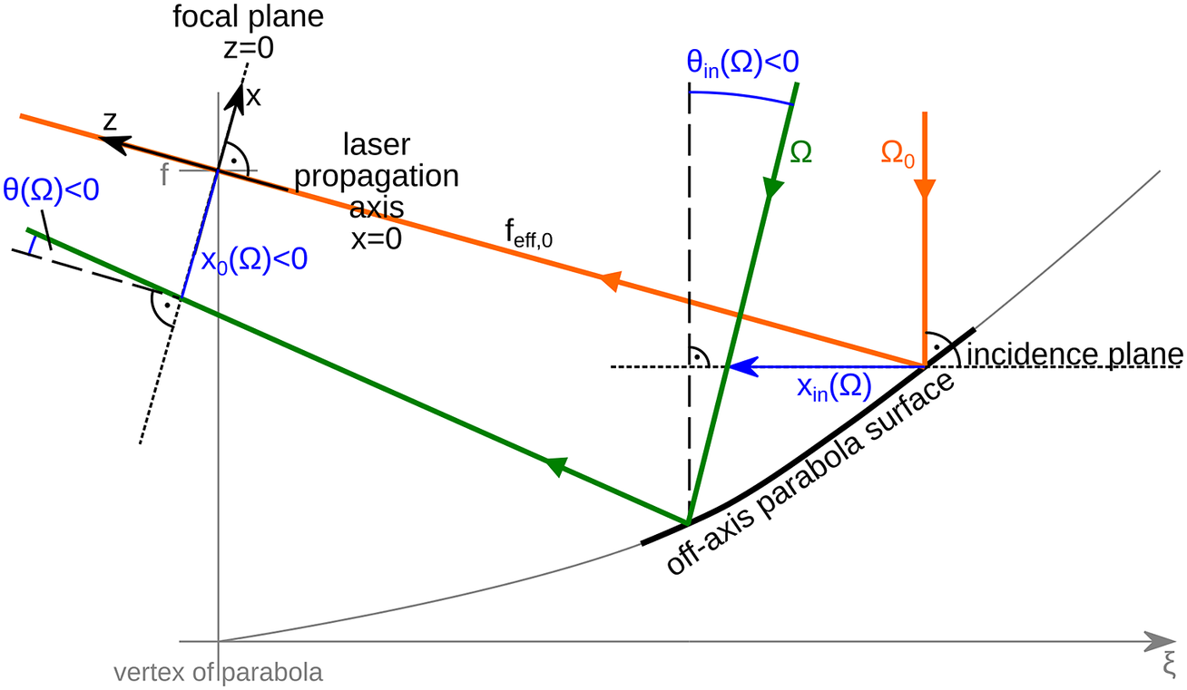
Figure 2 provides an overview of the geometry underlying the analytic calculations in the two steps. It visualizes important quantities used throughout the derivations.
Frequency–space domain visualization of the paths of two specific frequencies belonging to the spectrum of a Gaussian pulse that is under the influence of angular dispersion and spatial dispersion. These frequencies are transversally Gaussian distributed, and the rays represent the path of the respective distribution center. The pulse’s propagation direction is defined by the propagation direction $z$
of the central frequency
$z$
of the central frequency ${\Omega}_0$
. The propagation direction of frequency
${\Omega}_0$
. The propagation direction of frequency $\Omega$
encloses the angle
$\Omega$
encloses the angle $\theta \left(\Omega \right)$
with the central frequency’s propagation direction in the focal plane. This expresses immanent angular dispersion
$\theta \left(\Omega \right)$
with the central frequency’s propagation direction in the focal plane. This expresses immanent angular dispersion $\mathrm{AD}:= {\left.\frac{\mathrm{d}\theta }{\mathrm{d}\Omega}\right|}_{\Omega ={\Omega}_0}={\theta}^{\prime }$
of the focusing Gaussian pulse, which can originate from both angular dispersion
$\mathrm{AD}:= {\left.\frac{\mathrm{d}\theta }{\mathrm{d}\Omega}\right|}_{\Omega ={\Omega}_0}={\theta}^{\prime }$
of the focusing Gaussian pulse, which can originate from both angular dispersion ${\theta}_{\mathrm{in}}^{\prime}\left(\Omega \right)$
and spatial dispersion
${\theta}_{\mathrm{in}}^{\prime}\left(\Omega \right)$
and spatial dispersion ${x}_{\mathrm{in}}^{\prime}\left(\Omega \right)$
before the focusing off-axis parabola. In the focal plane
${x}_{\mathrm{in}}^{\prime}\left(\Omega \right)$
before the focusing off-axis parabola. In the focal plane $z=0$
, the spatial offset
$z=0$
, the spatial offset ${x}_{\mathrm{c}}={x}_0\left(\Omega \right)$
between the centers of beams
${x}_{\mathrm{c}}={x}_0\left(\Omega \right)$
between the centers of beams $\Omega$
and
$\Omega$
and ${\Omega}_0$
along the transverse direction
${\Omega}_0$
along the transverse direction $x$
expresses immanent spatial dispersion
$x$
expresses immanent spatial dispersion $\mathrm{SD}:= {\left.\frac{\mathrm{d}{x}_{\mathrm{c}}}{\mathrm{d}\Omega}\right|}_{\Omega ={\Omega}_0}={x}_0^{\prime }$
of the Gaussian pulse, which originates from angular dispersion before the off-axis parabola.
$\mathrm{SD}:= {\left.\frac{\mathrm{d}{x}_{\mathrm{c}}}{\mathrm{d}\Omega}\right|}_{\Omega ={\Omega}_0}={x}_0^{\prime }$
of the Gaussian pulse, which originates from angular dispersion before the off-axis parabola.
2 Deriving pulse properties during propagation
Our derivation of a laser pulse’s tilt angle, duration and width from given spatial, angular and higher-order dispersion starts by modeling the laser’s scalar electric field distribution in frequency space $\widehat{E}$
in the focal plane and propagating this to an arbitrary distance
$\widehat{E}$
in the focal plane and propagating this to an arbitrary distance $z$
from the focus using the Fresnel diffraction integral. We assume that the initial dispersion is present only along one axis in the transverse plane. This allows for a 2D formulation of laser propagation, where
$z$
from the focus using the Fresnel diffraction integral. We assume that the initial dispersion is present only along one axis in the transverse plane. This allows for a 2D formulation of laser propagation, where $x$
is the transverse direction and
$x$
is the transverse direction and $z$
is the laser propagation axis, on the basis of cylindrical waves in the following. This work can be extended to three dimensions by treating the other transverse direction (
$z$
is the laser propagation axis, on the basis of cylindrical waves in the following. This work can be extended to three dimensions by treating the other transverse direction ( $y$
) with cylindrical waves analogously.
$y$
) with cylindrical waves analogously.
2.1 Initial field in the focus in the frequency–space domain
We assume the laser frequency spectrum and transverse profile to be Gaussian in the focus:
 $$\begin{align*}\widehat{E}\left(x,z=0,\Omega \right)&={\epsilon}_{\Omega}{\epsilon}_x{e}^{- i\varphi},\\{\epsilon}_{\Omega}\left(\Omega \right)&={e}^{-\frac{\tau_0^2}{4}{\left(\Omega -{\Omega}_0\right)}^2},\\ {\epsilon}_x(x)&={e}^{-\frac{{\left(x-{x}_0\right)}^2}{w_0^2}},\end{align*}$$
where $\varphi =\varphi \left(x,z=0,\Omega \right)$
is the initial spectral phase of the pulse,
$\varphi =\varphi \left(x,z=0,\Omega \right)$
is the initial spectral phase of the pulse, $\Omega =2\pi \nu$
is the angular frequency,
$\Omega =2\pi \nu$
is the angular frequency, ${\Omega}_0$
is the central laser frequency,
${\Omega}_0$
is the central laser frequency, $\left(x,z\right)$
is the position considered with
$\left(x,z\right)$
is the position considered with $z=0$
marking the focus,
$z=0$
marking the focus, ${\tau}_0={\tau}_{\mathrm{FWHM},\mathrm{I}}/\sqrt{2\ln 2}$
is the Fourier limited duration,
${\tau}_0={\tau}_{\mathrm{FWHM},\mathrm{I}}/\sqrt{2\ln 2}$
is the Fourier limited duration, ${\tau}_{\mathrm{FWHM},\mathrm{I}}$
is the full width at half maximum of the field’s time–space domain longitudinal intensity distribution,
${\tau}_{\mathrm{FWHM},\mathrm{I}}$
is the full width at half maximum of the field’s time–space domain longitudinal intensity distribution, ${w}_0={w}_{\mathrm{FWHM},\mathrm{I}}/\sqrt{2\ln 2}$
is the focal width of the transverse spatial distribution of frequency
${w}_0={w}_{\mathrm{FWHM},\mathrm{I}}/\sqrt{2\ln 2}$
is the focal width of the transverse spatial distribution of frequency $\Omega$
,
$\Omega$
, ${w}_{\mathrm{FWHM},\mathrm{I}}$
is the focal full width at half maximum of the undisturbed pulse’s time–space domain transverse spatial intensity distribution and
${w}_{\mathrm{FWHM},\mathrm{I}}$
is the focal full width at half maximum of the undisturbed pulse’s time–space domain transverse spatial intensity distribution and ${x}_0={x}_0\left(\Omega \right)$
is the center position of the spatial distribution of frequency
${x}_0={x}_0\left(\Omega \right)$
is the center position of the spatial distribution of frequency $\Omega$
in the focus. The latter is related to spatial dispersion
$\Omega$
in the focus. The latter is related to spatial dispersion $\mathrm{SD}$
, being defined as the coefficient of the linear term in the expansion of the transverse frequency distribution center
$\mathrm{SD}$
, being defined as the coefficient of the linear term in the expansion of the transverse frequency distribution center ${x}_{\mathrm{c}}$
with respect to frequency:
${x}_{\mathrm{c}}$
with respect to frequency:
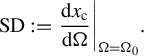 $$\begin{align}\mathrm{SD}:= {\left.\frac{\mathrm{d}{x}_{\mathrm{c}}}{\mathrm{d}\Omega}\right|}_{\Omega ={\Omega}_0}.\end{align}$$
Since ${x}_0={x}_{\mathrm{c}}\left(z=0\right)$
, the initial value of spatial dispersion at
${x}_0={x}_{\mathrm{c}}\left(z=0\right)$
, the initial value of spatial dispersion at $z=0$
is
$z=0$
is $\mathrm{SD}_{\mathrm{foc}}={x}_0^{\prime }$
.
$\mathrm{SD}_{\mathrm{foc}}={x}_0^{\prime }$
.
The laser’s spectral phase $\varphi \left(x,z=0,\Omega \right)$
in the focus is defined by the existence of angular dispersion in the focus
$\varphi \left(x,z=0,\Omega \right)$
in the focus is defined by the existence of angular dispersion in the focus $\mathrm{AD}_{\mathrm{foc}}$
. Angular dispersion manifests in the divergence of propagation directions between frequencies, where the propagation directions of frequency
$\mathrm{AD}_{\mathrm{foc}}$
. Angular dispersion manifests in the divergence of propagation directions between frequencies, where the propagation directions of frequency $\Omega$
and the central laser frequency
$\Omega$
and the central laser frequency ${\Omega}_0$
enclose the angle
${\Omega}_0$
enclose the angle $\theta =\theta \left(\Omega \right)$
. Similar to
$\theta =\theta \left(\Omega \right)$
. Similar to $\mathrm{SD}$
,
$\mathrm{SD}$
, $\mathrm{AD}$
is defined as the coefficient of the linear term in the expansion of
$\mathrm{AD}$
is defined as the coefficient of the linear term in the expansion of $\theta$
with respect to frequency:
$\theta$
with respect to frequency:
 $$\begin{align}\mathrm{AD}:= {\left.\frac{\mathrm{d}\theta }{\mathrm{d}\Omega}\right|}_{\Omega ={\Omega}_0}={\theta}^{\prime }.\end{align}$$
We deduce the laser’s initial spectral phase $\varphi$
from the spectral phase
$\varphi$
from the spectral phase $\phi$
of a plane wave of frequency
$\phi$
of a plane wave of frequency $\Omega$
propagating at an angle
$\Omega$
propagating at an angle $\theta$
with respect to the
$\theta$
with respect to the $z$
-axis:
$z$
-axis:
 $$\begin{align*}\phi \left(x,z,\Omega \right)=\frac{\Omega}{c}\left(-x\sin \theta +z\cos \theta \right).\end{align*}$$
Expanding this about $\Omega \approx {\Omega}_0$
and evaluating at the focus position
$\Omega \approx {\Omega}_0$
and evaluating at the focus position $z=0$
, the laser’s initial spectral phase
$z=0$
, the laser’s initial spectral phase $\varphi$
is obtained. Up to the third order it reads, cf. Appendix A.1,
$\varphi$
is obtained. Up to the third order it reads, cf. Appendix A.1,
 $$\begin{align*}&\varphi \left(x,z=0,\Omega \right)\approx -\frac{x}{c}{\Omega}_0{\theta}^{\prime}\left(\Omega -{\Omega}_0\right)-\frac{1}{2}\frac{x}{c}\left(2{\theta}^{\prime }+{\Omega}_0{\theta}^{{\prime\prime}}\right){\left(\Omega -{\Omega}_0\right)}^2\\& \qquad -\frac{1}{6}\frac{x}{c}\left(3{\theta}^{{\prime\prime} }+{\Omega}_0{\theta^{\prime\prime\prime} }-{\Omega}_0{\theta^{\prime}}^3\right){\left(\Omega -{\Omega}_0\right)}^3\\& \qquad +\frac{1}{2}{\mathrm{GDD}}_{\mathrm{foc}}{\left(\Omega -{\Omega}_0\right)}^2+\frac{1}{6}{\mathrm{TOD}}_{\mathrm{foc}}{\left(\Omega -{\Omega}_0\right)}^3\\& \quad =: -\alpha \frac{x}{w_0}+\frac{1}{2}{\mathrm{GDD}}_{\mathrm{foc}}{\left(\Omega -{\Omega}_0\right)}^2+\frac{1}{6}{\mathrm{TOD}}_{\mathrm{foc}}{\left(\Omega -{\Omega}_0\right)}^3,\end{align*}$$
where
 $$\begin{align}\alpha \left(\Omega \right)&=\frac{w_0}{c}\left[{\Omega}_0{\theta}^{\prime}\left(\Omega -{\Omega}_0\right)+\frac{1}{2}\left(2{\theta}^{\prime }+{\Omega}_0{\theta}^{{\prime\prime}}\right){\left(\Omega -{\Omega}_0\right)}^2\right. \nonumber\\& \qquad\quad \left.+\frac{1}{6}\left(3{\theta}^{{\prime\prime} }+{\Omega}_0{\theta^{\prime\prime\prime} }-{\Omega}_0{\theta^{\prime}}^3\right){\left(\Omega -{\Omega}_0\right)}^3\right].\end{align}$$
The quantity $\alpha /{w}_0$
can be regarded as the series expansion of a frequency’s wave vector
$\alpha /{w}_0$
can be regarded as the series expansion of a frequency’s wave vector $x$
-component,
$x$
-component, ${k}_x=-\left(\Omega /c\right)\sin \theta \left(\Omega \right)\approx -\alpha \left(\Omega \right)/{w}_0$
.
${k}_x=-\left(\Omega /c\right)\sin \theta \left(\Omega \right)\approx -\alpha \left(\Omega \right)/{w}_0$
.
The expansion of the spectral phase in the focus above includes values $\mathrm{GDD}_{\mathrm{foc}}$
and
$\mathrm{GDD}_{\mathrm{foc}}$
and $\mathrm{TOD}_{\mathrm{foc}}$
at
$\mathrm{TOD}_{\mathrm{foc}}$
at $z=0$
for group-delay dispersion and third-order dispersion in the focus, respectively. Generally, group-delay dispersion
$z=0$
for group-delay dispersion and third-order dispersion in the focus, respectively. Generally, group-delay dispersion $\mathrm{GDD}$
and third-order dispersion
$\mathrm{GDD}$
and third-order dispersion $\mathrm{TOD}$
are defined as follows:
$\mathrm{TOD}$
are defined as follows:
 $$\begin{align}\mathrm{GDD}:= {\left.\frac{{\mathrm{d}}^2\varphi }{\mathrm{d}{\Omega}^2}\right|}_{\Omega ={\Omega}_0},\end{align}$$
 $$\begin{align}\mathrm{TOD}:= {\left.\frac{{\mathrm{d}}^3\varphi }{\mathrm{d}{\Omega}^3}\right|}_{\Omega ={\Omega}_0},\end{align}$$
and evolve during propagation. Their values in the focus are determined from known values before the focusing mirror, emerging, for example, through material dispersion within the laser system, plus contributions from dispersion coupling through focusing, as will be shown later.
2.2 Field at some distance from the focus in the frequency–space domain
The field distribution outside the focus is obtained by propagating the initial field with the Fresnel diffraction integral for cylindrical waves[ Reference Siegmann 41 , Reference Steiniger, Widera, Pausch, Debus, Bussmann and Schramm 43 ], cf. Appendix A.2,
 $$\begin{align} &\widehat{E}\left(x,z,\Omega \right)=\sqrt{\frac{\Omega}{2\pi c}}\frac{e^{-i\left(\frac{\Omega}{c}z-\frac{\pi }{4}\right)}}{\sqrt{z}}\underset{-\infty }{\overset{\infty }{\int }}\widehat{E}\left(\xi, z=0,\Omega \right){e}^{-i\frac{\Omega}{2 cz}{\left(x-\xi \right)}^2}\kern0.1em \mathrm{d}\xi \nonumber\\&\quad =\sqrt{\frac{\Omega}{2\pi c}}\frac{e^{-i\left(\frac{\Omega}{c}z-\frac{\pi }{4}\right)}}{\sqrt{z}}{\epsilon}_{\Omega}{e}^{-i\frac{1}{2}{\mathrm{GDD}}_{\mathrm{foc}}{\left(\Omega -{\Omega}_0\right)}^2}{e}^{-i\frac{1}{6}{\mathrm{TOD}}_{\mathrm{foc}}{\left(\Omega -{\Omega}_0\right)}^3}\nonumber\\& \qquad \times\underset{-\infty }{\overset{\infty }{\int }}{\epsilon}_x\left(\xi \right){e}^{i\alpha \frac{\xi }{w_0}}{e}^{-i\frac{\Omega}{2 cz}{\left(x-\xi \right)}^2}\kern0.1em \mathrm{d}\xi \nonumber\\&\quad ={\epsilon}_{\Omega}{\left(1+\frac{z^2}{z_{\mathrm{R}}^2}\right)}^{-1/4}{e}^{-{\left[x-\left({x}_0-\frac{c}{\Omega_0{w}_0}\alpha z\right)\right]}^2\left[\frac{1}{w_0^2\left(1+{z}^2/{z}_{\mathrm{R}}^2\right)}+i\frac{\Omega}{2c}\frac{z}{\left({z}^2+{z}_{\mathrm{R}}^2\right)}\right]}\nonumber\\& \qquad \times {e}^{-i\frac{\Omega}{c}z}{e}^{i\alpha \frac{x}{w_0}}{e}^{i\frac{\alpha^2}{4}\frac{z}{z_{\mathrm{R}}}}{e}^{i\frac{1}{2}\arctan \frac{z}{z_{\mathrm{R}}}}{e}^{-i\frac{1}{2}{\mathrm{GDD}}_{\mathrm{foc}}{\left(\Omega -{\Omega}_0\right)}^2}\nonumber\\& \qquad \times {e}^{-i\frac{1}{6}{\mathrm{TOD}}_{\mathrm{foc}}{\left(\Omega -{\Omega}_0\right)}^3},\end{align}$$
where ${z}_{\mathrm{R}}=\Omega {w}_0^2/(2c)$
is the Rayleigh length,
${z}_{\mathrm{R}}=\Omega {w}_0^2/(2c)$
is the Rayleigh length, ${\lambda}_0=2\pi c/{\Omega}_0$
is the central laser wavelength and the well-known width
${\lambda}_0=2\pi c/{\Omega}_0$
is the central laser wavelength and the well-known width $w(z)$
and radius of curvature
$w(z)$
and radius of curvature $R(z)$
of the propagating laser pulse can be identified as
$R(z)$
of the propagating laser pulse can be identified as
 $$\begin{align}w(z)={w}_0\sqrt{1+\frac{z^2}{z_{\mathrm{R}}^2}},\end{align}$$
 $$\begin{align}R(z)=z\left(1+\frac{z_{\mathrm{R}}^2}{z^2}\right).\end{align}$$
While these expressions for $w$
and
$w$
and $R$
are frequency dependent in general, we set
$R$
are frequency dependent in general, we set ${z}_{\mathrm{R}}\approx \pi {w}_0^2/{\lambda}_0$
to good approximation in Equation (6) for the following calculations. Equation (6) is a well-known result[
Reference Akturk, Gu, Zeek and Trebino
44
]. See Appendix A for details of this and the following derivations.
${z}_{\mathrm{R}}\approx \pi {w}_0^2/{\lambda}_0$
to good approximation in Equation (6) for the following calculations. Equation (6) is a well-known result[
Reference Akturk, Gu, Zeek and Trebino
44
]. See Appendix A for details of this and the following derivations.
As is evident from the proportionality of the laser’s Gaussian transverse profile center ${x}_{\mathrm{c}}\left(z,\Omega \right)={x}_0-\alpha zc/\left({\Omega}_0{w}_0\right)$
to
${x}_{\mathrm{c}}\left(z,\Omega \right)={x}_0-\alpha zc/\left({\Omega}_0{w}_0\right)$
to $\alpha$
in Equation (6), a frequency’s spatial distribution center is subject to higher-order dispersion. From this, the scaling of spatial dispersion with distance from the focus can be derived using Equation (1), which reads to the first order as
$\alpha$
in Equation (6), a frequency’s spatial distribution center is subject to higher-order dispersion. From this, the scaling of spatial dispersion with distance from the focus can be derived using Equation (1), which reads to the first order as
 $$\begin{align*}\mathrm{SD}(z)={\mathrm{SD}}_{\mathrm{foc}}-{\mathrm{AD}}_{\mathrm{foc}}z.\end{align*}$$
Furthermore, Equation (6) allows identifying the advancement of higher-order dispersion with distance from the focus by performing the respective number of derivatives of the spectral phase $\varphi \left(x,z,\Omega \right)=- \mathrm{Arg}\left[\widehat{E}\left(x,z,\Omega \right)\right]$
with respect to
$\varphi \left(x,z,\Omega \right)=- \mathrm{Arg}\left[\widehat{E}\left(x,z,\Omega \right)\right]$
with respect to $\Omega$
and evaluating at
$\Omega$
and evaluating at $\Omega ={\Omega}_0$
. Accordingly, advancements of
$\Omega ={\Omega}_0$
. Accordingly, advancements of $\mathrm{GDD}$
and
$\mathrm{GDD}$
and $\mathrm{TOD}$
with
$\mathrm{TOD}$
with $z$
are obtained using Equations (4) and (5), respectively, cf. Appendix A.3,
$z$
are obtained using Equations (4) and (5), respectively, cf. Appendix A.3,
 $$\begin{align}\mathrm{GDD}(z)={\mathrm{GDD}}_{\mathrm{foc}}+4\frac{x}{w}{\beta}_3{\beta}_5+2{\Omega}_0\left(2\frac{x}{w}{\beta}_4+{\beta}_3^2\right){\beta}_5-2{\beta}_6,\end{align}$$
 $$\begin{align}\mathrm{TOD}(z)&={\mathrm{TOD}}_{\mathrm{foc}}+12\frac{x}{w}{\beta}_4{\beta}_5+6{\beta}_3^2{\beta}_5+12{\Omega}_0\frac{x}{w}{\beta}_5{\delta}_1\nonumber\\& \quad +12{\Omega}_0{\beta}_3{\beta}_4{\beta}_5-6{\delta}_2,\end{align}$$
where
 $$\begin{align*}{\delta}_1&=\frac{z}{6w{\Omega}_0}\left(3{\theta}^{{\prime\prime} }+{\Omega}_0{\theta^{\prime\prime\prime} }-{\Omega}_0{\theta^{\prime}}^3-{x^{\prime\prime\prime}}_0\right),\\[2pt]{\delta}_2&=\frac{1}{2c}\left[{\theta}^{\prime}\left(2{\theta}^{\prime }+{\Omega}_0{\theta}^{{\prime\prime}}\right)z+\frac{1}{3}\left(3{\theta}^{{\prime\prime} }+{\Omega}_0{\theta^{\prime\prime\prime} }-{\Omega}_0{\theta^{\prime}}^3\right)x\right],\end{align*}$$
making use of the definitions in Equation (13) given below.
Equations (9) and (10) are more complex than those typically used[
Reference Akturk, Gu, Zeek and Trebino
44
] and exhibit a variation over the transverse pulse profile either due to angular dispersion or the combination of spatial dispersion and diffraction or both. Moreover, even along the laser propagation axis ( $x=0$
) spatial dispersion contributes to group-delay dispersion:
$x=0$
) spatial dispersion contributes to group-delay dispersion:
 $$\begin{align}{\left. \mathrm{GDD}(z)\right|}_{x=0}={\mathrm{GDD}}_{\mathrm{foc}}+\frac{\Omega_0}{c}\frac{\mathrm{SD}{(z)}^2}{R}-\frac{\Omega_0}{c}{\mathrm{AD}}_{\mathrm{foc}}^2z.\end{align}$$
This contribution compensates phase run-up outside the focus for off-axis traveling frequencies by taking phase front curvature into account. Phase run-up outside the focus originates from the term proportional to $\mathrm{AD}_{\mathrm{foc}}^2z$
, which itself represents a correction of phase due to a corrected traveling distance for off-axis traveling frequencies. Since this traveling distance correction is based upon a plane wave assumption, it is only valid near the focus, where
$\mathrm{AD}_{\mathrm{foc}}^2z$
, which itself represents a correction of phase due to a corrected traveling distance for off-axis traveling frequencies. Since this traveling distance correction is based upon a plane wave assumption, it is only valid near the focus, where $z\ll {z}_{\mathrm{R}}$
, and the correction by the term
$z\ll {z}_{\mathrm{R}}$
, and the correction by the term $\propto {\mathrm{SD}}^2/R$
is necessary. Far from the focus, where
$\propto {\mathrm{SD}}^2/R$
is necessary. Far from the focus, where $z\gg {z}_{\mathrm{R}}$
and
$z\gg {z}_{\mathrm{R}}$
and $R(z)\approx z$
, the two corrections cancel each other out in the case of vanishing spatial dispersion in the focus:
$R(z)\approx z$
, the two corrections cancel each other out in the case of vanishing spatial dispersion in the focus: ${\left. \mathrm{GDD}\left(z\gg {z}_{\mathrm{R}}\right)\right|}_{x=0,{\mathrm{SD}}_{\mathrm{foc}}=0}={\mathrm{GDD}}_{\mathrm{foc}}$
.
${\left. \mathrm{GDD}\left(z\gg {z}_{\mathrm{R}}\right)\right|}_{x=0,{\mathrm{SD}}_{\mathrm{foc}}=0}={\mathrm{GDD}}_{\mathrm{foc}}$
.
The above form of the initial field in the focus $E\left(x,z=0,\Omega \right)$
assumes that all frequencies focus at the same position
$E\left(x,z=0,\Omega \right)$
assumes that all frequencies focus at the same position $z=0$
along the central frequency’s propagation direction. This holds as long as the phase fronts of the expanded laser pulse, which is focused by the OAP, are flat. Typically this requires keeping the distance between the last telescope in the laser system and the OAP well below the Rayleigh range of the expanded laser pulse. If this is not the case, chromatic aberration will occur and further distort the pulse, as has been studied for focusing by a lens[
Reference Federico and Martinez
45
].
$z=0$
along the central frequency’s propagation direction. This holds as long as the phase fronts of the expanded laser pulse, which is focused by the OAP, are flat. Typically this requires keeping the distance between the last telescope in the laser system and the OAP well below the Rayleigh range of the expanded laser pulse. If this is not the case, chromatic aberration will occur and further distort the pulse, as has been studied for focusing by a lens[
Reference Federico and Martinez
45
].
2.3 Field at some distance from the focus in the time–space domain
The field distribution in the time–space domain is obtained by Fourier transforming the above field distribution in the frequency domain (Equation (6)) to the time domain:
 $$\begin{align*}E\left(x,z,t\right)=\frac{1}{2\pi}\int \widehat{E}\left(x,z,\Omega \right){e}^{i\Omega t}\mathrm{d}\Omega .\end{align*}$$
The result presented in the following allows for the first time to read off analytical relations for the scaling of pulse-front tilt and pulse duration valid in the close vicinity, as well as far from the focus.
In order to perform the Fourier transform, the in-focus transverse distribution center ${x}_0$
of a frequency is expanded up to the second order,
${x}_0$
of a frequency is expanded up to the second order, ${x}_0\approx {x}_0^{\prime}\left(\Omega -{\Omega}_0\right)+\frac{1}{2}{x}_0^{{\prime\prime} }{\left(\Omega -{\Omega}_0\right)}^2$
, and the definition in Equation (3) of
${x}_0\approx {x}_0^{\prime}\left(\Omega -{\Omega}_0\right)+\frac{1}{2}{x}_0^{{\prime\prime} }{\left(\Omega -{\Omega}_0\right)}^2$
, and the definition in Equation (3) of $\alpha$
is inserted in the complex argument of Equation (6), allowing one to order terms in powers of
$\alpha$
is inserted in the complex argument of Equation (6), allowing one to order terms in powers of $\Omega -{\Omega}_0$
. Neglecting every contribution of the third order and higher, cf. Equations (98)–(129) in Appendix A.3,
$\Omega -{\Omega}_0$
. Neglecting every contribution of the third order and higher, cf. Equations (98)–(129) in Appendix A.3,
 $$\begin{align} &\widehat{E}\left(x,z,\Omega \right)={\left(1+\frac{z^2}{z_{\mathrm{R}}^2}\right)}^{-1/4}{e}^{-\frac{x^2}{w^2}}{e}^{-i{\Omega}_0\frac{x^2}{2 cR}}{e}^{-i\frac{\Omega_0}{c}z}{e}^{i\frac{1}{2}\arctan \frac{z}{z_{\mathrm{R}}}}\nonumber\\& \quad \times {e}^{-\left[\left({\beta}_1+2\frac{x}{w}{\beta}_4+{\beta}_3^2\right)+i\left(\frac{1}{2}{\mathrm{GDD}}_{\mathrm{foc}}+2\frac{x}{w}{\beta}_3{\beta}_5+\left(2\frac{x}{w}{\beta}_4+{\beta}_3^2\right){\Omega}_0{\beta}_5-{\beta}_6\right)\right]{\left(\Omega -{\Omega}_0\right)}^2}\nonumber\\& \quad \times {e}^{-\left[2\frac{x}{w}{\beta}_3+i\left({\beta}_2+\frac{x^2}{w^2}{\beta}_5+2{\Omega}_0\frac{x}{w}{\beta}_3{\beta}_5\right)\right]\left(\Omega -{\Omega}_0\right)},\end{align}$$
where
 $$\begin{align} {\beta}_1&=\frac{\tau_0^2}{4}\nonumber,\\{\beta}_2&=\frac{z}{c}-{\Omega}_0{\theta}^{\prime}\frac{x}{c}\nonumber,\\{\beta}_3&=-\frac{\mathrm{SD}(z)}{w}\nonumber,\\{\beta}_4&=\frac{1}{2w}\left(2{\theta}^{\prime}\frac{z}{\Omega_0}+{\Omega}_0{\theta}^{{\prime\prime}}\frac{z}{\Omega_0}-{x}_0^{{\prime\prime}}\right)\nonumber,\\{\beta}_5&=\frac{w^2}{2 cR}\nonumber,\\{\beta}_6&=\frac{1}{2c}\left[{\Omega}_0{\theta^{\prime}}^2z+\left(2{\theta}^{\prime }+{\Omega}_0{\theta}^{{\prime\prime}}\right)x\right],\end{align}$$
and the approximated field can be analytically transformed to the time domain. The assumption of vanishing third- and higher-order dispersion for a particular setup can be verified with the help of Equation (123) from Appendix A. From this, it becomes clear that third-order contributions to the envelope and phase are negligible if $128\cdot \left[\left(x/w\right){\delta}_1+{\beta}_3{\beta}_4\right]/ {\tau}_0^3\ll 1$
and
$128\cdot \left[\left(x/w\right){\delta}_1+{\beta}_3{\beta}_4\right]/ {\tau}_0^3\ll 1$
and $11\cdot \mathrm{TOD}(z)/{\tau}_0^3\ll 1$
, respectively, which assumes that the spectral amplitude is only significant for frequencies
$11\cdot \mathrm{TOD}(z)/{\tau}_0^3\ll 1$
, respectively, which assumes that the spectral amplitude is only significant for frequencies $\left|\Omega -{\Omega}_0\right|\le 4/{\tau}_0$
(the amplitude falls below
$\left|\Omega -{\Omega}_0\right|\le 4/{\tau}_0$
(the amplitude falls below ${e}^{-4}$
of its initial value for a larger frequency deviation). In practice, these requirements are fulfilled for standard high-power, ultra-short laser pulses. For example, the requirements take absolute values of
${e}^{-4}$
of its initial value for a larger frequency deviation). In practice, these requirements are fulfilled for standard high-power, ultra-short laser pulses. For example, the requirements take absolute values of $3\times {10}^{-6}$
and
$3\times {10}^{-6}$
and $1\times {10}^{-6}$
, respectively, when evaluated at a Rayleigh length distance from the focus at the pulse center for a pulse of wavelength
$1\times {10}^{-6}$
, respectively, when evaluated at a Rayleigh length distance from the focus at the pulse center for a pulse of wavelength ${\lambda}_0=800$
nm and duration
${\lambda}_0=800$
nm and duration ${\tau}_{\mathrm{FWHM},\mathrm{I}}=5$
fs (
${\tau}_{\mathrm{FWHM},\mathrm{I}}=5$
fs ( ${\tau}_0=4.25$
fs), being tightly focused to
${\tau}_0=4.25$
fs), being tightly focused to ${w}_0=2$
μm and angularly dispersed in the focus
${w}_0=2$
μm and angularly dispersed in the focus $\mathrm{AD}_{\mathrm{foc}}=1$
μrad/nm.
$\mathrm{AD}_{\mathrm{foc}}=1$
μrad/nm.
Further defining
 $$\begin{align*} {\gamma}_1&=1+8\frac{x}{w}\frac{\beta_4}{\tau_0^2}+4\frac{\beta_3^2}{\tau_0^2},\\{\gamma}_2&=\left[\frac{1}{2}{\mathrm{GDD}}_{\mathrm{foc}}+2\frac{x}{w}{\beta}_3{\beta}_5+\left(2\frac{x}{w}{\beta}_4+{\beta}_3^2\right){\Omega}_0{\beta}_5-{\beta}_6\right]\frac{4}{\tau_0^2}\\&= \mathrm{GDD}(z)\frac{2}{\tau_0^2},\\{\gamma}_3&=-2\frac{x}{w}\frac{\beta_3}{\tau_0}=2\frac{\mathrm{SD}(z)}{w^2{\tau}_0}x,\\{\gamma}_4&=\left(t-{\beta}_2-\frac{x^2}{w^2}{\beta}_5-2{\Omega}_0\frac{x}{w}{\beta}_3{\beta}_5\right)\frac{1}{\tau_0},\end{align*}$$
allows to write the field in the time domain in a compact form. The time–space domain field is, cf. Equations (130)–(135) in Appendix A.3,
 $$\begin{align} E\left(x,z,t\right)&=\frac{1}{\tau_0\sqrt{\pi }}{\left[\left(1+\frac{z^2}{z_{\mathrm{R}}^2}\right)\left({\gamma}_1^2+{\gamma}_2^2\right)\right]}^{-1/4}{e}^{i{\Omega}_0\left(t-\frac{z}{c}-\frac{x^2}{2 cR}\right)}\nonumber\\& \quad \times {e}^{i\frac{1}{2}\left(\arctan \frac{z}{z_{\mathrm{R}}}-\arctan \frac{\gamma_2}{\gamma_1}\right)} {e}^{-\frac{x^2}{w^2{\gamma}_1}\left(1+8\frac{x}{w}{\beta}_4/{\tau}_0^2\right)}\nonumber\\& \quad \times {e}^{-\frac{{\left[{\tau}_0{\gamma}_4-\frac{\left({\tau}_0{\gamma}_3\right)\left({\tau}_0^2{\gamma}_2\right)}{\tau_0^2{\gamma}_1}\right]}^2}{\tau_0^2\left({\gamma}_1+{\gamma}_2^2/{\gamma}_1\right)}}{e}^{i\frac{\left({\gamma}_4^2-{\gamma}_3^2\right){\gamma}_2+2{\gamma}_3{\gamma}_4{\gamma}_1}{{\gamma}_1^2+{\gamma}_2^2}},\nonumber\\[-14pt] \end{align}$$
provided ${\gamma}_1>0$
, otherwise the Fourier transform over the Gaussian spectrum cannot be performed analytically since the frequency–space domain field (Equation (12)) grows exponentially with
${\gamma}_1>0$
, otherwise the Fourier transform over the Gaussian spectrum cannot be performed analytically since the frequency–space domain field (Equation (12)) grows exponentially with ${\left(\Omega -{\Omega}_0\right)}^2$
. For a detailed explanation, see Appendix A.3, Equation (130). Future work may model the spectrum with a different function in order to remove the requirement
${\left(\Omega -{\Omega}_0\right)}^2$
. For a detailed explanation, see Appendix A.3, Equation (130). Future work may model the spectrum with a different function in order to remove the requirement ${\gamma}_1>0$
.
${\gamma}_1>0$
.
The only problematic term with respect to the requirement ${\gamma}_1>0$
is the middle term in
${\gamma}_1>0$
is the middle term in ${\gamma}_1$
being proportional to
${\gamma}_1$
being proportional to ${\beta}_4$
, which also appears in the nominator of the exponent of the transverse profile scaling as
${\beta}_4$
, which also appears in the nominator of the exponent of the transverse profile scaling as ${e}^{-{x}^2}$
in Equation (14). In general, this term cannot be neglected and its contribution can become significant in certain regimes, for example, for pulses with a duration of the order of only a few femtoseconds or shorter. These regimes demand to verify
${e}^{-{x}^2}$
in Equation (14). In general, this term cannot be neglected and its contribution can become significant in certain regimes, for example, for pulses with a duration of the order of only a few femtoseconds or shorter. These regimes demand to verify ${\gamma}_1>0$
when using the analytic expression for the total field or those for the pulse’s spatio-temporal properties further below.
${\gamma}_1>0$
when using the analytic expression for the total field or those for the pulse’s spatio-temporal properties further below.
There is, however, the ‘long pulse’ regime where the term proportional to ${\beta}_4$
can be neglected and
${\beta}_4$
can be neglected and ${\gamma}_1$
remains positive always. In this regime,
${\gamma}_1$
remains positive always. In this regime, $\left|8{\beta}_4/{\tau}_0^2\right|\ll 1$
, which can be rewritten as
$\left|8{\beta}_4/{\tau}_0^2\right|\ll 1$
, which can be rewritten as $8\pi \left|{\Omega}_0{\mathrm{AD}}_{\mathrm{foc}}\right|\left({w}_0/{\lambda}_0\right){\left({\Omega}_0{\tau}_0\right)}^{-2}\ll 1$
, with
$8\pi \left|{\Omega}_0{\mathrm{AD}}_{\mathrm{foc}}\right|\left({w}_0/{\lambda}_0\right){\left({\Omega}_0{\tau}_0\right)}^{-2}\ll 1$
, with $\left|{\Omega}_0{\mathrm{AD}}_{\mathrm{foc}}\right|=\left|\tan {\psi}_{\mathrm{tilt},{\mathrm{AD}}_{\mathrm{foc}}}\right|$
representing pulse-front tilt in the focus due to
$\left|{\Omega}_0{\mathrm{AD}}_{\mathrm{foc}}\right|=\left|\tan {\psi}_{\mathrm{tilt},{\mathrm{AD}}_{\mathrm{foc}}}\right|$
representing pulse-front tilt in the focus due to $\mathrm{AD}_{\mathrm{foc}}$
alone. That is, the middle term proportional to
$\mathrm{AD}_{\mathrm{foc}}$
alone. That is, the middle term proportional to ${\beta}_4$
will not be of relevance in
${\beta}_4$
will not be of relevance in ${\gamma}_1$
as long as the
${\gamma}_1$
as long as the $\mathrm{AD}_{\mathrm{foc}}$
induced angle of pulse-front tilt
$\mathrm{AD}_{\mathrm{foc}}$
induced angle of pulse-front tilt ${\psi}_{\mathrm{tilt},{\mathrm{AD}}_{\mathrm{foc}}}$
satisfies
${\psi}_{\mathrm{tilt},{\mathrm{AD}}_{\mathrm{foc}}}$
satisfies $\left|\tan {\psi}_{\mathrm{tilt},{\mathrm{AD}}_{\mathrm{foc}}}\right|\ll {\lambda}_0{\left({\Omega}_0{\tau}_0\right)}^2/\left(8\pi {w}_0\right)$
, meaning that the tilt angle needs to be of the order of the ratio of the pulse duration (measured in number of laser oscillations) over the pulse width (measured in wavelengths) and provided that the pulse duration extends over several laser oscillations. Exemplarily, for a
$\left|\tan {\psi}_{\mathrm{tilt},{\mathrm{AD}}_{\mathrm{foc}}}\right|\ll {\lambda}_0{\left({\Omega}_0{\tau}_0\right)}^2/\left(8\pi {w}_0\right)$
, meaning that the tilt angle needs to be of the order of the ratio of the pulse duration (measured in number of laser oscillations) over the pulse width (measured in wavelengths) and provided that the pulse duration extends over several laser oscillations. Exemplarily, for a ${\lambda}_0=0.8$
μm,
${\lambda}_0=0.8$
μm, ${\tau}_{\mathrm{FWHM},\mathrm{I}}=30$
fs (
${\tau}_{\mathrm{FWHM},\mathrm{I}}=30$
fs ( ${\tau}_0=25.5$
fs) pulse with a focal width of
${\tau}_0=25.5$
fs) pulse with a focal width of $\pi {w}_0\equiv 60{\lambda}_0$
, the ‘long pulse’ regime is reached if
$\pi {w}_0\equiv 60{\lambda}_0$
, the ‘long pulse’ regime is reached if ${\psi}_{\mathrm{tilt},{\mathrm{AD}}_{\mathrm{foc}}}\ll {82}^{\circ }$
, and the requirement relaxes further for smaller focal spot diameters.
${\psi}_{\mathrm{tilt},{\mathrm{AD}}_{\mathrm{foc}}}\ll {82}^{\circ }$
, and the requirement relaxes further for smaller focal spot diameters.
To our knowledge, the term $8\left(x/w\right)\left({\beta}_4/{\tau}_0^2\right)$
in
$8\left(x/w\right)\left({\beta}_4/{\tau}_0^2\right)$
in ${\gamma}_1$
has not been taken into account in previous analysis of spatio-temporal couplings and its appearance outside the long pulse regime could only be recognized from the fully analytic treatment presented here.
${\gamma}_1$
has not been taken into account in previous analysis of spatio-temporal couplings and its appearance outside the long pulse regime could only be recognized from the fully analytic treatment presented here.
While expressions for typically interesting intensity-related pulse parameters are derived from the time–space domain field (Equation (14)) in the following, it has several more areas of applicability. For example, one can derive the phase-related wavefront rotation[ Reference Akturk, Gu, Gabolde and Trebino 29 ] or feed the field into self-consistent simulations of pulse propagation or laser–matter interaction.
2.4 Duration, width and tilt of the propagating pulse
From Equation (14) the duration $T$
and width
$T$
and width $W$
of the propagating Gaussian laser pulse with spatial, angular and group-delay dispersion in the focus are readily identified. These are the denominators of the fractions in the exponents of the last and next to last real exponential:
$W$
of the propagating Gaussian laser pulse with spatial, angular and group-delay dispersion in the focus are readily identified. These are the denominators of the fractions in the exponents of the last and next to last real exponential:
 $$\begin{align}{\tau}^2&={\tau}_0^2{\gamma}_1={\tau}_0^2\left[1+8\frac{x}{w}\frac{\beta_4}{\tau_0^2}+4\frac{\mathrm{SD}{(z)}^2}{w^2{\tau}_0^2}\right], \end{align}$$
 $$\begin{align}{T}^2&={\tau}_0^2\left({\gamma}_1+\frac{\gamma_2^2}{\gamma_1}\right)={\tau}^2+4\frac{\mathrm{GDD}{(z)}^2}{\tau^2},\end{align}$$
 $$\begin{align}{W}^2&={w}^2\frac{\tau^2}{\tau_0^2+8\frac{x}{w}{\beta}_4}.\end{align}$$
However, $W$
generally is not a typical Gaussian pulse width, as it still depends on the transverse coordinate
$W$
generally is not a typical Gaussian pulse width, as it still depends on the transverse coordinate $x$
. This rather shows that the transverse envelope does not keep a Gaussian shape during propagation but evolves to something more complex. (By setting
$x$
. This rather shows that the transverse envelope does not keep a Gaussian shape during propagation but evolves to something more complex. (By setting $x=W$
in Equation (17) and solving the resulting cubic equation in
$x=W$
in Equation (17) and solving the resulting cubic equation in $W/w$
it is possible to yield a value for
$W/w$
it is possible to yield a value for $W$
that corresponds to its original meaning for a Gaussian beam, that is, as the distance from the pulse center along the transverse direction where the intensity reduces to
$W$
that corresponds to its original meaning for a Gaussian beam, that is, as the distance from the pulse center along the transverse direction where the intensity reduces to $1/{e}^2$
compared to its center value.) Yet, these deviations from a Gaussian profile are not of relevance in the long pulse regime where the term proportional to
$1/{e}^2$
compared to its center value.) Yet, these deviations from a Gaussian profile are not of relevance in the long pulse regime where the term proportional to ${\beta}_4$
can be neglected. Then
${\beta}_4$
can be neglected. Then $W$
quantifies the width of a normal Gaussian transverse profile. That is, the laser pulse keeps a Gaussian transverse profile and the spatio-temporal couplings do not alter the transverse profile to something more complex during propagation.
$W$
quantifies the width of a normal Gaussian transverse profile. That is, the laser pulse keeps a Gaussian transverse profile and the spatio-temporal couplings do not alter the transverse profile to something more complex during propagation.
The expression for pulse duration (Equation (16)) is structurally equal to previously published results[
Reference Akturk, Gu, Zeek and Trebino
44
], but comprises more complex expressions for $\tau$
and
$\tau$
and $\mathrm{GDD}(z)$
, Equations (15) and (9), respectively. In the long pulse regime,
$\mathrm{GDD}(z)$
, Equations (15) and (9), respectively. In the long pulse regime, $\tau$
assumes the well-known form
$\tau$
assumes the well-known form ${\tau}^2={\tau}_0^2+4 \mathrm{SD}{(z)}^2/{w}^2$
, and represents pulse elongation due to spatial dispersion alone. In cases where pulse elongation takes place via group velocity dispersion in a dispersive material, the proportion of spatial dispersion is zero and
${\tau}^2={\tau}_0^2+4 \mathrm{SD}{(z)}^2/{w}^2$
, and represents pulse elongation due to spatial dispersion alone. In cases where pulse elongation takes place via group velocity dispersion in a dispersive material, the proportion of spatial dispersion is zero and $\tau ={\tau}_0$
.
$\tau ={\tau}_0$
.
From the numerator of the exponent of the last real exponential in Equation (14) the time delay ${t}_0$
of the pulse maximum can be identified:
${t}_0$
of the pulse maximum can be identified:
 $$\begin{align*}{\tau}_0{\gamma}_4-\frac{\left({\tau}_0{\gamma}_3\right)\left({\tau}_0^2{\gamma}_2\right)}{\tau_0^2{\gamma}_1}=: t-{t}_0,\end{align*}$$
where
 $$\begin{align*}{t}_0=\frac{z}{c}-{\Omega}_0{\mathrm{AD}}_{\mathrm{foc}}\frac{x}{c}+\frac{x^2}{2 cR}-\frac{\Omega_0}{c}\frac{\mathrm{SD}(z)}{R}x+4\frac{\mathrm{SD}(z)}{w^2}\frac{\mathrm{GDD}(z)}{\tau^2}x.\end{align*}$$
The time delay is directly connected to the pulse-front tilt by
 $$\begin{align*}\tan {\psi}_{\mathrm{tilt}}={\left.\frac{\mathrm{d}\left({ct}_0\right)}{\mathrm{d}x}\right|}_{x=0},\end{align*}$$
which yields, cf. Appendix A.4,
 $$\begin{align}\tan {\psi}_{\mathrm{tilt}}=-{\Omega}_0{\mathrm{AD}}_{\mathrm{foc}}-{\Omega}_0\frac{\mathrm{SD}(z)}{R}+4c\frac{\mathrm{SD}(z)}{w^2}{\left[\frac{\mathrm{GDD}(z)}{\tau^2}\right]}_{x=0}.\end{align}$$
In this expression, the first term represents a constant base value of pulse-front tilt due to angular dispersion, which is the true value of pulse-front tilt in the center of the focal plane[ Reference Martinez 27 ]. The remaining terms represent deviations from the focal plane center value due to radial offset of the point of evaluation or pulse propagation.
The second term is zero in the focus, but non-zero outside. For a specific frequency, it represents an effective angle of propagation due to increasing SD during propagation, just as AD represents an angle of propagation. It can be the major source of pulse-front tilt outside the focus, as observed for the setups in the next section. Its derivation is a main result of this work.
The structure of the third term is in line with previous findings[
Reference Akturk, Gu, Zeek and Trebino
44
]. However, the definition for ${\left. \mathrm{GDD}(z)\right|}_{x=0}$
is extended in this work by the contribution of spatial dispersion, that is, the term proportional to
${\left. \mathrm{GDD}(z)\right|}_{x=0}$
is extended in this work by the contribution of spatial dispersion, that is, the term proportional to $\mathrm{SD}^2/R$
in Equation (11).
$\mathrm{SD}^2/R$
in Equation (11).
Note that the definition of pulse-front tilt is not unique. The above definition is with respect to time delay ${t}_0$
of the pulse maximum along the transverse direction at some position
${t}_0$
of the pulse maximum along the transverse direction at some position $z$
, but pulse-front tilt can be defined with respect to longitudinal spatial offset
$z$
, but pulse-front tilt can be defined with respect to longitudinal spatial offset ${z}_0$
between the pulse maximum and pulse center along the transverse direction at some time
${z}_0$
between the pulse maximum and pulse center along the transverse direction at some time $t$
, too. The relation between the two definitions is
$t$
, too. The relation between the two definitions is
 $$\begin{align*}\tan {\alpha}_{\mathrm{tilt}}={\left.\frac{\mathrm{d}\left({z}_0\right)}{\mathrm{d}x}\right|}_{x=0}=-\tan {\psi}_{\mathrm{tilt}}.\end{align*}$$
3 Deriving pulse dispersion in the focus of an off-axis parabola
Using the above formulas to estimate pulse properties during propagation of a tightly focused laser pulse requires knowledge about the dispersion in the focus. Usually, these dispersion properties in the focus are unknown but estimated from the dispersion properties before the focusing mirror, where these can be measured. Using a ray tracing approach, dispersion parameters in the focus are derived in the following from the known dispersion parameters before focusing, which couple during reflection at the focusing mirror. We denote parameters before focusing with subscript ‘in’, and parameters in the focus with subscript ‘foc,coupl’. The in-focus dispersion values derived in this section will be used in the next section as input for the in-focus dispersion values in the pulse parameter formulas, Equations (18) and (16), where the latter are denoted with subscript ‘foc’.
We will assume focusing of the laser pulse at an OAP, as is standard for high-power laser systems. The pulse has only first-order contributions ${x}_{\mathrm{in}}^{\prime }$
and
${x}_{\mathrm{in}}^{\prime }$
and ${\theta}_{\mathrm{in}}^{\prime }$
to spatial and angular dispersion, respectively, before focusing. Group-delay dispersion before focusing
${\theta}_{\mathrm{in}}^{\prime }$
to spatial and angular dispersion, respectively, before focusing. Group-delay dispersion before focusing ${\mathrm{GDD}}_{\mathrm{in}}$
is not explicitly taken into account as it does not evolve, but can simply be added to the in-focus value of group-delay dispersion
${\mathrm{GDD}}_{\mathrm{in}}$
is not explicitly taken into account as it does not evolve, but can simply be added to the in-focus value of group-delay dispersion $\mathrm{GDD}_{\mathrm{foc},\mathrm{coupl}}$
, that is,
$\mathrm{GDD}_{\mathrm{foc},\mathrm{coupl}}$
, that is, ${\mathrm{GDD}}_{\mathrm{foc}}={\mathrm{GDD}}_{\mathrm{foc},\mathrm{coupl}}+{\mathrm{GDD}}_{\mathrm{in}}$
, and similar for
${\mathrm{GDD}}_{\mathrm{foc}}={\mathrm{GDD}}_{\mathrm{foc},\mathrm{coupl}}+{\mathrm{GDD}}_{\mathrm{in}}$
, and similar for ${\mathrm{TOD}}_{\mathrm{foc}}$
. Obtaining estimates for dispersion-coupling induced in-focus values of spatial dispersion
${\mathrm{TOD}}_{\mathrm{foc}}$
. Obtaining estimates for dispersion-coupling induced in-focus values of spatial dispersion ${\mathrm{SD}}_{\mathrm{foc},\mathrm{coupl}}$
, angular dispersion
${\mathrm{SD}}_{\mathrm{foc},\mathrm{coupl}}$
, angular dispersion ${\mathrm{AD}}_{\mathrm{foc},\mathrm{coupl}}$
, group-delay dispersion
${\mathrm{AD}}_{\mathrm{foc},\mathrm{coupl}}$
, group-delay dispersion ${\mathrm{GDD}}_{\mathrm{foc},\mathrm{coupl}}$
and third-order dispersion
${\mathrm{GDD}}_{\mathrm{foc},\mathrm{coupl}}$
and third-order dispersion ${\mathrm{TOD}}_{\mathrm{foc},\mathrm{coupl}}$
relies on analytic tracing of rays representing the propagation of the center of a frequency’s transverse spatial distribution. Figure 3 sketches sample rays and defines all quantities used in the following derivation of dispersion properties in the focus.
${\mathrm{TOD}}_{\mathrm{foc},\mathrm{coupl}}$
relies on analytic tracing of rays representing the propagation of the center of a frequency’s transverse spatial distribution. Figure 3 sketches sample rays and defines all quantities used in the following derivation of dispersion properties in the focus.
Propagation of rays of different frequency during focusing of a laser pulse at an OAP. The central frequency’s incident ray (orange) propagates parallel to the axis of the OAP. The incidence plane is perpendicular to the ray and located at the point of incidence of the ray on the OAP surface. The ray encloses with the OAP’s surface normal the angle $\delta$
, which determines the angle of deflection
$\delta$
, which determines the angle of deflection ${\psi}_{\mathrm{defl},0}=2\delta$
. During subsequent propagation into the focus, the central frequency ray covers the effective focal distance
${\psi}_{\mathrm{defl},0}=2\delta$
. During subsequent propagation into the focus, the central frequency ray covers the effective focal distance ${f}_{\mathrm{eff},0}=f/{\cos}^2\left({\psi}_{\mathrm{defl},0}/2\right)$
. The focal plane is perpendicular to the central frequency ray and located in the OAP’s focus. A second ray belonging to frequency
${f}_{\mathrm{eff},0}=f/{\cos}^2\left({\psi}_{\mathrm{defl},0}/2\right)$
. The focal plane is perpendicular to the central frequency ray and located in the OAP’s focus. A second ray belonging to frequency $\Omega$
(green) encloses the angle
$\Omega$
(green) encloses the angle ${\theta}_{\mathrm{in}}$
with the central frequency ray and has a transverse spatial offset of
${\theta}_{\mathrm{in}}$
with the central frequency ray and has a transverse spatial offset of ${x}_{\mathrm{in}}$
at the incidence plane. The propagation angle
${x}_{\mathrm{in}}$
at the incidence plane. The propagation angle ${\theta}_{\mathrm{in}}$
is negative in this setup. Compared to the central frequency ray, the second ray propagates an additional distance
${\theta}_{\mathrm{in}}$
is negative in this setup. Compared to the central frequency ray, the second ray propagates an additional distance ${L}_{\mathrm{in}}$
until it is incident on the mirror surface. Its deflection angle
${L}_{\mathrm{in}}$
until it is incident on the mirror surface. Its deflection angle ${\psi}_{\mathrm{defl}}$
, effective focal distance
${\psi}_{\mathrm{defl}}$
, effective focal distance ${f}_{\mathrm{eff}}$
, propagation angle
${f}_{\mathrm{eff}}$
, propagation angle $\theta$
and propagation distance until the focal plane
$\theta$
and propagation distance until the focal plane ${L}_{\mathrm{foc}}$
differ from the central frequency ray. The point where the second ray pierces the focal plane defines its transverse spatial offset
${L}_{\mathrm{foc}}$
differ from the central frequency ray. The point where the second ray pierces the focal plane defines its transverse spatial offset ${x}_0$
.
${x}_0$
.

3.1 Angular dispersion
In the focus, the rays of frequency $\Omega$
and
$\Omega$
and ${\Omega}_0$
enclose the propagation angle
${\Omega}_0$
enclose the propagation angle $\theta$
being required to calculate angular dispersion by Equation (2). The propagation angle is determined from the difference between the angles enclosed by the OAP’s optical axis and the deflected rays of
$\theta$
being required to calculate angular dispersion by Equation (2). The propagation angle is determined from the difference between the angles enclosed by the OAP’s optical axis and the deflected rays of $\Omega$
and
$\Omega$
and ${\Omega}_0$
. Since there is angular dispersion already present before deflection at the mirror, the angle enclosed by the deflected ray of frequency
${\Omega}_0$
. Since there is angular dispersion already present before deflection at the mirror, the angle enclosed by the deflected ray of frequency $\Omega$
and the OAP’s optical axis is
$\Omega$
and the OAP’s optical axis is ${\psi}_{\mathrm{defl}}-{\theta}_{\mathrm{in}}$
, which leads to
${\psi}_{\mathrm{defl}}-{\theta}_{\mathrm{in}}$
, which leads to
 $$\begin{align*}\theta \left(\Omega \right)={\psi}_{\mathrm{defl}}-{\theta}_{\mathrm{in}}-{\psi}_{\mathrm{defl},0}.\end{align*}$$
The deflection angle of frequency $\Omega$
is given by
$\Omega$
is given by
 $$\begin{align}{\psi}_{\mathrm{defl}}=2\delta,\end{align}$$
where the tangent of $\delta$
can be determined from the slope of the mirror surface at the position of incidence
$\delta$
can be determined from the slope of the mirror surface at the position of incidence $\xi$
:
$\xi$
:
 $$\begin{align}\delta =\arctan \frac{\xi }{2f}.\end{align}$$
The position of incidence is obtained by computing the intersection point between the ray and the mirror surface, that is, by equating
 $$\begin{align*}\left({z}_{\mathrm{ray}}+\frac{\xi_0^2}{4f}\right)\tan {\theta}_{\mathrm{in}}=\xi -\left({\xi}_0-{x}_{\mathrm{in}}\right) \quad\mathrm{and}\quad {z}_{\mathrm{OAP}}=-\frac{\xi^2}{4f},\end{align*}$$
where the $z$
-axis points along the axis of propagation of the incident central frequency ray but originates at the vertex of the parabola. The resulting equation for the incidence position is
$z$
-axis points along the axis of propagation of the incident central frequency ray but originates at the vertex of the parabola. The resulting equation for the incidence position is
 $$\begin{align*} 0&=\frac{\tan {\theta}_{\mathrm{in}}}{4f}{\xi}^2+\xi -\left({\xi}_0-{x}_{\mathrm{in}}\right)-\frac{\tan {\theta}_{\mathrm{in}}}{4f}{\xi}_0^2\\\iff 0&=a\frac{\xi^2}{f^2}+b\frac{\xi }{f}+c,\end{align*}$$
where
 $$\begin{align*}a&=\frac{\tan {\theta}_{\mathrm{in}}}{4},\\b&=1,\\c&=-\frac{\xi_0-{x}_{\mathrm{in}}}{f}-\frac{\tan {\theta}_{\mathrm{in}}}{4}\frac{\xi_0^2}{f^2}. \end{align*}$$
This quadratic equation in $\xi /f$
has the solution
$\xi /f$
has the solution
 $$\begin{align} \kern-12pt\xi &=2f\frac{-1+\sqrt{1-\tan {\theta}_{\mathrm{in}}c}}{\tan {\theta}_{\mathrm{in}}}\nonumber\\&\approx p+\left(q-\frac{p^2}{4f}\right){\theta}_{\mathrm{in}},\ \mathrm{where}\;p={\xi}_0-{x}_{\mathrm{in}}\;\mathrm{and}\;q=\frac{\xi_0^2}{4f},\end{align}$$
with which $\delta$
and thus
$\delta$
and thus ${\psi}_{\mathrm{defl}}$
can be calculated for any frequency
${\psi}_{\mathrm{defl}}$
can be calculated for any frequency $\Omega$
, cf. Equations (20) and (19), respectively. We assume
$\Omega$
, cf. Equations (20) and (19), respectively. We assume ${\xi}_0$
to be given from the manufactured deflection angle and effective focal distance for the central frequency:
${\xi}_0$
to be given from the manufactured deflection angle and effective focal distance for the central frequency:
 $$\begin{align*}{\xi}_0={f}_{\mathrm{eff},0}\sin {\psi}_{\mathrm{defl},0}.\end{align*}$$
With the above solution for the incidence point on the parabola surface, angular dispersion in the focus can be calculated:
 $$\begin{align}\mathrm{AD}_{\mathrm{foc},\mathrm{coupl}}&=\frac{\mathrm{d}}{\mathrm{d}\Omega}{\left[2\arctan \left(\frac{\xi }{2f}\right)-{\theta}_{\mathrm{in}}-{\psi}_{\mathrm{d}\mathrm{efl},0}\right]}_{\Omega ={\Omega}_0}\nonumber\\ &=-\frac{1}{f_{\mathrm{eff},0}}{x}_{\mathrm{in}}^{\prime }-{\theta}_{\mathrm{in}}^{\prime }.\end{align}$$
3.2 Spatial dispersion
Calculating spatial dispersion according to Equation (1) requires one to determine the spatial offset ${x}_0$
of frequency
${x}_0$
of frequency $\Omega$
in the focal plane. According to Figure 3, the spatial offset
$\Omega$
in the focal plane. According to Figure 3, the spatial offset ${x}_0$
can be determined from
${x}_0$
can be determined from ${\tilde{x}}_0$
:
${\tilde{x}}_0$
:
 $$\begin{align*}{x}_0=\frac{{\tilde{x}}_0}{\cos \theta },\end{align*}$$
which is itself determined by ${\tilde{x}}_0={f}_{\mathrm{eff}}\sin {\theta}_{\mathrm{in}}$
. Thus,
${\tilde{x}}_0={f}_{\mathrm{eff}}\sin {\theta}_{\mathrm{in}}$
. Thus,
 $$\begin{align}\mathrm{SD}_{\mathrm{foc},\mathrm{coupl}}=\frac{\mathrm{d}}{\mathrm{d}\Omega}{\left(\frac{f_{\mathrm{eff}}\sin {\theta}_{\mathrm{in}}}{\cos \theta}\right)}_{\Omega ={\Omega}_0}={f}_{\mathrm{eff},0}{\theta}_{\mathrm{in}}^{\prime }.\end{align}$$
3.3 Group-delay dispersion
Calculating group-delay dispersion according to Equation (4) requires one to determine the phase advance of every frequency from the incidence plane to the focal plane, which can be calculated from a frequency’s optical path length. The path of a ray starts where its phase front intersects with the incidence position of the central frequency ray on the mirror surface and it ends where its phase front intersects with the focus (see Figure 3). The path length of a frequency $\Omega$
is divided into two sections,
$\Omega$
is divided into two sections, ${L}_{\mathrm{in}}$
and
${L}_{\mathrm{in}}$
and ${L}_{\mathrm{foc}}$
. The former is the distance from the starting point until the ray intersects with the parabola surface, while the latter is the distance from the parabola surface until the focal plane. The phase advance is
${L}_{\mathrm{foc}}$
. The former is the distance from the starting point until the ray intersects with the parabola surface, while the latter is the distance from the parabola surface until the focal plane. The phase advance is
 $$\begin{align}\varphi \left(\Omega \right)=\frac{\Omega}{c}\left({L}_{\mathrm{in}}+{L}_{\mathrm{foc}}\right),\end{align}$$
where
 $$\begin{align*}{L}_{\mathrm{in}}\left(\Omega \right)=-{x}_{\mathrm{in}}\sin {\theta}_{\mathrm{in}}+\frac{\xi_0^2-{\xi}^2}{4f\cos {\theta}_{\mathrm{in}}},\kern1em {L}_{\mathrm{foc}}\left(\Omega \right)={f}_{\mathrm{eff}}\cos {\theta}_{\mathrm{in}}, \end{align*}$$
with which
 $$\begin{align}\mathrm{GDD}_{\mathrm{foc},\mathrm{coupl}}={\left.\frac{{\mathrm{d}}^2\varphi }{\mathrm{d}{\Omega}^2}\right|}_{\Omega ={\Omega}_0}=-\frac{\Omega_0}{c}\left({f}_{\mathrm{eff},0}{\theta_{\mathrm{in}}^{\prime}}^2+2{\theta}_{\mathrm{in}}^{\prime }{x}_{\mathrm{in}}^{\prime}\right).\end{align}$$
3.4 Third-order dispersion
For future real and numerical experiments the value of third-order dispersion in the focus can be of interest. It is evaluated by applying Equation (5) on the phase advance (Equation (24)):
 $$\begin{align}\mathrm{TOD}_{\mathrm{foc},\mathrm{coupl}}={\left.\frac{{\mathrm{d}}^3\varphi }{\mathrm{d}{\Omega}^3}\right|}_{\Omega ={\Omega}_0}=3\frac{\theta_{\mathrm{in}}^{\prime }}{c}\left({\Omega}_0{\xi}_0\frac{\theta_{\mathrm{in}}^{\prime }{x}_{\mathrm{in}}^{\prime }}{f}-{f}_{\mathrm{eff},0}{\theta}_{\mathrm{in}}^{\prime }-2{x}_{\mathrm{in}}^{\prime}\right).\end{align}$$
4 Showcasing pulse-front tilt and pulse duration scaling
In exemplary long and short focal range setups, pulse-front tilt and pulse duration during propagation of a focusing pulse through its focus are presented in the following. As is shown, pulse-front tilts can become several tens of degrees large in the close vicinity of a couple of tens of micrometers around the focus. Pulse-front tilts of this order were observed in previous numerical experiments[ Reference Zhang, Asoubar, Kammel, Nolte and Wyrowski 8 ], but could not be fully analytically explained.
The laser pulse is focused at an OAP, and for the calculation we assume that dispersion parameters before reflection at the OAP, that is, angular dispersion $\mathrm{AD}_{\mathrm{in}}$
and spatial dispersion
$\mathrm{AD}_{\mathrm{in}}$
and spatial dispersion $\mathrm{SD}_{\mathrm{in}}$
, are known. From these, the dispersion values in the focus are deduced by Equations (22), (23) and (25) using
$\mathrm{SD}_{\mathrm{in}}$
, are known. From these, the dispersion values in the focus are deduced by Equations (22), (23) and (25) using ${\theta}_{\mathrm{in}}=\mathrm{AD}_{\mathrm{in}}$
and
${\theta}_{\mathrm{in}}=\mathrm{AD}_{\mathrm{in}}$
and ${x}_{\mathrm{in}}^{\prime}=\mathrm{SD}_{\mathrm{in}}$
. The in-focus dispersion values
${x}_{\mathrm{in}}^{\prime}=\mathrm{SD}_{\mathrm{in}}$
. The in-focus dispersion values $\mathrm{AD}_{\mathrm{foc},\mathrm{coupl}}$
,
$\mathrm{AD}_{\mathrm{foc},\mathrm{coupl}}$
, $\mathrm{SD}_{\mathrm{foc},\mathrm{coupl}}$
and
$\mathrm{SD}_{\mathrm{foc},\mathrm{coupl}}$
and $\mathrm{GDD}_{\mathrm{foc},\mathrm{coupl}}$
, respectively, are then plugged into Equations (16) and (18) in order to determine pulse duration and tilt, respectively, during propagation.
$\mathrm{GDD}_{\mathrm{foc},\mathrm{coupl}}$
, respectively, are then plugged into Equations (16) and (18) in order to determine pulse duration and tilt, respectively, during propagation.
All setups will use a laser pulse with a central wavelength ${\lambda}_0=0.8$
μm, duration
${\lambda}_0=0.8$
μm, duration ${\tau}_{\mathrm{FWHM},\mathrm{I}}=30$
fs and width
${\tau}_{\mathrm{FWHM},\mathrm{I}}=30$
fs and width ${D}_{\mathrm{in}}=\pi {w}_{\mathrm{in}}=100$
mm (99% power transmission through an aperture of this diameter for Gaussian beams) before focusing.
${D}_{\mathrm{in}}=\pi {w}_{\mathrm{in}}=100$
mm (99% power transmission through an aperture of this diameter for Gaussian beams) before focusing.
4.1 Short focal length setup
This setup’s OAP has ${f}_{\mathrm{eff},0}/{D}_{\mathrm{in}}=2.5$
(
${f}_{\mathrm{eff},0}/{D}_{\mathrm{in}}=2.5$
( $=f/\#$
), focusing the incident pulse to a width
$=f/\#$
), focusing the incident pulse to a width ${w}_{\mathrm{FWHM},\mathrm{I}}=2.35$
μm and resulting in a Rayleigh length
${w}_{\mathrm{FWHM},\mathrm{I}}=2.35$
μm and resulting in a Rayleigh length ${z}_{\mathrm{R}}=16$
μm.
${z}_{\mathrm{R}}=16$
μm.
Figure 4 visualizes pulse-front tilt and pulse duration in the course of propagation through the focus for angular dispersion values before focusing ranging from $\mathrm{AD}_{\mathrm{in}}=5\times {10}^{-3}$
to 1 μrad/nm without spatial dispersion before focusing, that is,
$\mathrm{AD}_{\mathrm{in}}=5\times {10}^{-3}$
to 1 μrad/nm without spatial dispersion before focusing, that is, $\mathrm{SD}_{\mathrm{in}}=0$
. While small values of
$\mathrm{SD}_{\mathrm{in}}=0$
. While small values of $\mathrm{AD}_{\mathrm{in}}$
below
$\mathrm{AD}_{\mathrm{in}}$
below ${10}^{-2}$
μrad/nm result in a maximum pulse-front tilt of
${10}^{-2}$
μrad/nm result in a maximum pulse-front tilt of $-{3.6}^{\circ }$
at a Rayleigh length before the focus, higher values such as
$-{3.6}^{\circ }$
at a Rayleigh length before the focus, higher values such as $0.25$
μrad/nm result in a large maximum pulse-front tilt of
$0.25$
μrad/nm result in a large maximum pulse-front tilt of $-{51}^{\circ }$
at about the same position. Angular dispersion before focusing of 1 μrad/nm results in an even larger maximum pulse-front tilt of
$-{51}^{\circ }$
at about the same position. Angular dispersion before focusing of 1 μrad/nm results in an even larger maximum pulse-front tilt of $-{61}^{\circ }$
at
$-{61}^{\circ }$
at $3.5$
Rayleigh lengths before the focus. Generally, it can be observed that larger values of
$3.5$
Rayleigh lengths before the focus. Generally, it can be observed that larger values of $\mathrm{AD}_{\mathrm{in}}$
result in larger maximum pulse-front tilt farther away from the focus. In all of these examples, group-delay dispersion in the focus
$\mathrm{AD}_{\mathrm{in}}$
result in larger maximum pulse-front tilt farther away from the focus. In all of these examples, group-delay dispersion in the focus $\mathrm{GDD}_{\mathrm{foc},\mathrm{coupl}}$
due to
$\mathrm{GDD}_{\mathrm{foc},\mathrm{coupl}}$
due to $\mathrm{AD}_{\mathrm{in}}$
is negligible, as it is only
$\mathrm{AD}_{\mathrm{in}}$
is negligible, as it is only $-0.2$
fs
$-0.2$
fs ${}^2$
for the largest
${}^2$
for the largest $\mathrm{AD}_{\mathrm{in}}$
. To ease comparison to the numerical results shown later, the in-focus value
$\mathrm{AD}_{\mathrm{in}}$
. To ease comparison to the numerical results shown later, the in-focus value $\mathrm{GDD}_{\mathrm{foc}}$
is therefore set to zero in the calculations.
$\mathrm{GDD}_{\mathrm{foc}}$
is therefore set to zero in the calculations.
Pulse-front tilt and pulse duration in the course of propagation of a $0.8$
μm,
$0.8$
μm, ${\tau}_{\mathrm{FWHM},\mathrm{I}}=30$
fs,
${\tau}_{\mathrm{FWHM},\mathrm{I}}=30$
fs, ${D}_{\mathrm{in}}=100$
mm laser pulse through the focus of the short focal range setup without spatial dispersion before the focusing mirror. The colors of the lines represent angular dispersion values before focusing
${D}_{\mathrm{in}}=100$
mm laser pulse through the focus of the short focal range setup without spatial dispersion before the focusing mirror. The colors of the lines represent angular dispersion values before focusing $\mathrm{AD}_{\mathrm{in}}=5\times {10}^{-3},1\times {10}^{-2},\mathrm{2.5}\times {10}^{-2},5\times {10}^{-2},\mathrm{0.1,0.25,0.5,1}$
μrad/nm. Originating from
$\mathrm{AD}_{\mathrm{in}}=5\times {10}^{-3},1\times {10}^{-2},\mathrm{2.5}\times {10}^{-2},5\times {10}^{-2},\mathrm{0.1,0.25,0.5,1}$
μrad/nm. Originating from $\mathrm{AD}_{\mathrm{in}}$
, there is angular dispersion, and hence pulse-front tilt, in the focus
$\mathrm{AD}_{\mathrm{in}}$
, there is angular dispersion, and hence pulse-front tilt, in the focus $\mathrm{AD}_{\mathrm{foc}}=-\mathrm{AD}_{\mathrm{in}}$
. Correspondingly, the position of zero pulse-front tilt along the beamline is outside the focus, as shown in the inset. Since absolute values of pulse-front tilt in the focus
$\mathrm{AD}_{\mathrm{foc}}=-\mathrm{AD}_{\mathrm{in}}$
. Correspondingly, the position of zero pulse-front tilt along the beamline is outside the focus, as shown in the inset. Since absolute values of pulse-front tilt in the focus $\mid {\psi}_{\mathrm{tilt}}\mid$
are below
$\mid {\psi}_{\mathrm{tilt}}\mid$
are below ${0.05}^{\circ }$
for all values of
${0.05}^{\circ }$
for all values of $\mathrm{AD}_{\mathrm{in}}$
, this offset is negligible in practice for this particular example.
$\mathrm{AD}_{\mathrm{in}}$
, this offset is negligible in practice for this particular example.

The major source of these large pulse-front tilts is the appearance of spatial dispersion, that is, the term $-{\Omega}_0 \mathrm{SD}/R$
in Equation (18). In this term,
$-{\Omega}_0 \mathrm{SD}/R$
in Equation (18). In this term, $\mathrm{SD}$
and
$\mathrm{SD}$
and $R$
together define a maximum propagation angle, which at the same time is the maximum angle enclosed by a phase front and the laser propagation axis. Just as for
$R$
together define a maximum propagation angle, which at the same time is the maximum angle enclosed by a phase front and the laser propagation axis. Just as for $-{\Omega}_0{\theta}^{\prime }$
, this angle leads to a maximum time delay along the transverse direction and therefore pulse-front tilt. This pulse-front tilt caused by spatial dispersion varies during propagation due to the varying radius of curvature
$-{\Omega}_0{\theta}^{\prime }$
, this angle leads to a maximum time delay along the transverse direction and therefore pulse-front tilt. This pulse-front tilt caused by spatial dispersion varies during propagation due to the varying radius of curvature $R$
. It reaches its maximum at a Rayleigh length from the focus, where the respective time delay is largest due to
$R$
. It reaches its maximum at a Rayleigh length from the focus, where the respective time delay is largest due to $R$
being smallest, and it vanishes in the focus where
$R$
being smallest, and it vanishes in the focus where $R$
is infinite such that there is no time delay.
$R$
is infinite such that there is no time delay.
The third term in Equation (18) constitutes a damping of the leading second term. For larger angular dispersion before focusing it provides for the shift of maximum pulse-front tilt to positions beyond the Rayleigh length, which is the position where the second term peaks.
In contrast to pulse-front tilt, the increase of pulse duration is only relevant for the two largest $\mathrm{AD}_{\mathrm{in}}$
values, with a maximum of
$\mathrm{AD}_{\mathrm{in}}$
values, with a maximum of $3.5{\tau}_0$
in the focus for
$3.5{\tau}_0$
in the focus for $\mathrm{AD}_{\mathrm{in}}=1$
μrad/nm.
$\mathrm{AD}_{\mathrm{in}}=1$
μrad/nm.
The source of pulse elongation is again spatial dispersion, described by Equation (15) alone since $\mathrm{GDD}$
is assumed to vanish in the focus. Spatial dispersion leads to a loss of overlap between spatial distributions of frequencies, which thins out the local spectrum. This effect is largest in the focus where the spatial frequency distributions are smallest, and thus the local spectrum is smallest and the pulse duration is longest.
$\mathrm{GDD}$
is assumed to vanish in the focus. Spatial dispersion leads to a loss of overlap between spatial distributions of frequencies, which thins out the local spectrum. This effect is largest in the focus where the spatial frequency distributions are smallest, and thus the local spectrum is smallest and the pulse duration is longest.
The above setup neglects $\mathrm{SD}_{\mathrm{in}}$
, that is, spatial dispersion generated by angular dispersion during propagation from the laser system’s compressor until the OAP. Assuming 10 m distance from the compressor until the OAP, spatial dispersion before focusing at the OAP due to propagation with angular dispersion is
$\mathrm{SD}_{\mathrm{in}}$
, that is, spatial dispersion generated by angular dispersion during propagation from the laser system’s compressor until the OAP. Assuming 10 m distance from the compressor until the OAP, spatial dispersion before focusing at the OAP due to propagation with angular dispersion is $\mathrm{SD}_{\mathrm{in}}=-\mathrm{AD}_{\mathrm{in}}\cdot 10\ \mathrm{m}={-}0.05,{-}0.1,{-}0.25,{-}0.5,{-}1,{-}2.5,{-}5,{-}10$
μm/nm. This spatial dispersion before focusing will not influence spatial dispersion in the focus, according to Equation (23), but it will increase angular dispersion, and therefore pulse-front tilt, in the focus. Pulse-front tilts in the focus are
$\mathrm{SD}_{\mathrm{in}}=-\mathrm{AD}_{\mathrm{in}}\cdot 10\ \mathrm{m}={-}0.05,{-}0.1,{-}0.25,{-}0.5,{-}1,{-}2.5,{-}5,{-}10$
μm/nm. This spatial dispersion before focusing will not influence spatial dispersion in the focus, according to Equation (23), but it will increase angular dispersion, and therefore pulse-front tilt, in the focus. Pulse-front tilts in the focus are ${\psi}_{\mathrm{tilt}}=\mathrm{0.01}^{\circ},\mathrm{0.02}^{\circ},\mathrm{0.04}^{\circ},\mathrm{0.09}^{\circ},\mathrm{0.18}^{\circ},\mathrm{0.45}^{\circ},\mathrm{0.90}^{\circ},\mathrm{1.79}^{\circ}$
, respectively. Since these are still small, the overall picture of the scaling remains equal compared to the setup with
${\psi}_{\mathrm{tilt}}=\mathrm{0.01}^{\circ},\mathrm{0.02}^{\circ},\mathrm{0.04}^{\circ},\mathrm{0.09}^{\circ},\mathrm{0.18}^{\circ},\mathrm{0.45}^{\circ},\mathrm{0.90}^{\circ},\mathrm{1.79}^{\circ}$
, respectively. Since these are still small, the overall picture of the scaling remains equal compared to the setup with $\mathrm{SD}_{\mathrm{in}}=0$
. In particular, maximum values of pulse-front tilt and duration do not change.
$\mathrm{SD}_{\mathrm{in}}=0$
. In particular, maximum values of pulse-front tilt and duration do not change.
4.2 Long focal range setup
This setup’s OAP has ${f}_{\mathrm{eff},0}/{D}_{\mathrm{in}}=250$
, focusing the incident pulse to a width
${f}_{\mathrm{eff},0}/{D}_{\mathrm{in}}=250$
, focusing the incident pulse to a width ${w}_{\mathrm{FWHM},\mathrm{I}}=19$
μm and resulting in a Rayleigh length
${w}_{\mathrm{FWHM},\mathrm{I}}=19$
μm and resulting in a Rayleigh length ${z}_{\mathrm{R}}=1.0$
mm.
${z}_{\mathrm{R}}=1.0$
mm.
Figure 5 visualizes pulse-front tilt and pulse duration in the course of propagation through the focus for the same range of angular dispersion values before focusing as for the short focal range setup and without spatial dispersion before focusing. Due to equal laser parameters, the scaling is qualitatively equal to the short focal range setup. Only the maximum value of pulse-front tilt is reduced, since the radius of the pulse-front curvature scales quadratically in the focal distance while spatial dispersion scales linearly for equal laser parameters before focusing. In total, this results in less time delay between frequencies along the transverse direction, reducing pulse-front tilt.
Pulse-front tilt and pulse duration in the course of propagation through the focus of the long focal range setup without spatial dispersion before focusing. Parameters are equal to the short focal range setup (see Figure 4).

Pulse duration in focus remains equal between long and short focal range setups, as the ratio of spatial dispersion and width in focus, which determines pulse elongation, is independent of focal length.
The considerations for group-delay dispersion in the focus and spatial dispersion before focusing outlined for the short focal range setup can be identically applied to this long focal range setup.
5 Comparing analytical results with numerical simulations
The obtained pulse-front tilt and pulse duration of the short focal range setup are cross-checked by numerically Fourier transforming the propagated pulse in Fourier space (Equation (6)) for the setup with $\mathrm{AD}_{\mathrm{in}}=1$
μrad/nm and measuring pulse-front tilt and pulse duration from the obtained time–space domain spatio-temporal intensity envelope on a grid. This intensity envelope is obtained from the complex field distribution by taking the absolute square. Taking from this 2D intensity distribution two 1D intensity distributions at constant transverse positions
$\mathrm{AD}_{\mathrm{in}}=1$
μrad/nm and measuring pulse-front tilt and pulse duration from the obtained time–space domain spatio-temporal intensity envelope on a grid. This intensity envelope is obtained from the complex field distribution by taking the absolute square. Taking from this 2D intensity distribution two 1D intensity distributions at constant transverse positions ${x}_{\mathrm{center}}$
and
${x}_{\mathrm{center}}$
and ${x}_{\mathrm{out}}$
allows for measuring pulse-front tilt. We chose
${x}_{\mathrm{out}}$
allows for measuring pulse-front tilt. We chose ${x}_{\mathrm{center}}=0$
and
${x}_{\mathrm{center}}=0$
and ${x}_{\mathrm{out}}={w}_0$
. By determining the respective times
${x}_{\mathrm{out}}={w}_0$
. By determining the respective times ${t}_{\mathrm{center}}$
and
${t}_{\mathrm{center}}$
and ${t}_{\mathrm{out}}$
at which the intensity reaches its maximum along these two 1D intensity distributions, the pulse-front tilt angle can be approximated by
${t}_{\mathrm{out}}$
at which the intensity reaches its maximum along these two 1D intensity distributions, the pulse-front tilt angle can be approximated by
 $$\begin{align}\tan {\psi}_{\mathrm{tilt},\mathrm{num}}=\frac{c\left({t}_{\mathrm{center}}-{t}_{\mathrm{out}}\right)}{x_{\mathrm{center}}-{x}_{\mathrm{out}}}.\end{align}$$
Pulse duration is measured by the least square fit of a Gaussian curve ${I}_0\exp \left[-{\left(t-{t}_{\mathrm{center}}\right)}^2/\left(2{\sigma}^{2}\right)\right]$
to the 1D intensity distribution at
${I}_0\exp \left[-{\left(t-{t}_{\mathrm{center}}\right)}^2/\left(2{\sigma}^{2}\right)\right]$
to the 1D intensity distribution at ${x}_{\mathrm{center}}$
, where
${x}_{\mathrm{center}}$
, where ${I}_0$
equals the maximum of the intensity distribution. The fit determines
${I}_0$
equals the maximum of the intensity distribution. The fit determines ${\sigma}_{I,t}$
, which is related to the pulse duration of the field by
${\sigma}_{I,t}$
, which is related to the pulse duration of the field by $T=2{\sigma}_{I,t}$
.
$T=2{\sigma}_{I,t}$
.
Figure 6 visualizes intensity envelope distributions at different distances $z$
from the focus together with measured and predicted contours for the pulse front as well as measured values of pulse-front tilt and duration. Agreement between measured and predicted values can be observed, from which we conclude successful verification of the analytic formulas derived in this work.
$z$
from the focus together with measured and predicted contours for the pulse front as well as measured values of pulse-front tilt and duration. Agreement between measured and predicted values can be observed, from which we conclude successful verification of the analytic formulas derived in this work.
Distribution of the time–space domain intensity envelope along the transverse direction $x$
and time
$x$
and time $t$
at different distances
$t$
at different distances $z$
from the focus. Pulse parameters are equal to Figure 4 with
$z$
from the focus. Pulse parameters are equal to Figure 4 with $\mathrm{AD}_{\mathrm{in}}=1$
μrad/nm. All distributions are normalized to the respective expected maximum value in the focus
$\mathrm{AD}_{\mathrm{in}}=1$
μrad/nm. All distributions are normalized to the respective expected maximum value in the focus $E{\left(x=0,z=0,t=0\right)}^2$
, cf. Equation (6). Colored lines mark pulse-front contours as expected from analytic and numeric determination of the pulse-front tilt angle, Equations (18) and (27), respectively. In addition, the duration of the field envelope is provided, which is obtained from the least square fit of a Gaussian curve to the 1D intensity distribution along
$E{\left(x=0,z=0,t=0\right)}^2$
, cf. Equation (6). Colored lines mark pulse-front contours as expected from analytic and numeric determination of the pulse-front tilt angle, Equations (18) and (27), respectively. In addition, the duration of the field envelope is provided, which is obtained from the least square fit of a Gaussian curve to the 1D intensity distribution along $x=0$
.
$x=0$
.

The remaining differences between measured and predicted values originate from finite sampling of the intensity distribution along the $t$
-axis. The arrival time of the intensity maximum at some
$t$
-axis. The arrival time of the intensity maximum at some $x$
can only be determined with an uncertainty about the size of the time sampling step, which results in an uncertainty on the pulse-front tilt angle. It is of the order of one degree or less in our setup.
$x$
can only be determined with an uncertainty about the size of the time sampling step, which results in an uncertainty on the pulse-front tilt angle. It is of the order of one degree or less in our setup.
Note, since the pulse’s width in the focus is significantly smaller than its length, the visible envelope ellipse is not aligned with the drawn contour of the pulse front. However, for each $x$
the highest intensity is indeed on this contour, which just defines this contour as the pulse front. Further note that the difference in the analytically calculated absolute value of the pulse-front tilt angle between
$x$
the highest intensity is indeed on this contour, which just defines this contour as the pulse front. Further note that the difference in the analytically calculated absolute value of the pulse-front tilt angle between $z=-{z}_{\mathrm{R}}$
and
$z=-{z}_{\mathrm{R}}$
and $z={z}_{\mathrm{R}}$
originates from the fact that the position where the pulse-front tilt vanishes is slightly behind the focus at
$z={z}_{\mathrm{R}}$
originates from the fact that the position where the pulse-front tilt vanishes is slightly behind the focus at $z>0$
.
$z>0$
.
6 Conclusions
We presented analytical expressions allowing one to evaluate the electric field, width, duration and tilt of dispersive, tightly focused, short pulse, Gaussian lasers in the vicinity and far from their focus in the time–space domain, which was not possible before. With the help of these expressions we were able to link the appearance of large pulse-front tilts of several tens of degrees, observed within a few Rayleigh lengths distance from the focus of a laser pulse featuring only weak angular dispersion, to the accompanying spatial dispersion. Numerical evaluation of the tilt and duration of Gaussian pulses propagated in simulations verified the predictions provided by the analytic expressions, which proves their applicability.
The possibility of generating large pulse-front tilts in the vicinity of the laser’s focus with moderate to low pulse elongation is thereby interesting on its own, as generating and utilizing pulses with large pulse-front tilts becomes simpler in ‘out-of-focus’ interaction geometries without the cost of large pulse elongation usually connected to large pulse-front tilt.
Moreover, the presented analytic expressions of the dispersion variation during propagation or of the full electric field can be of general use, for example, to simply estimate pulse properties at any position along the beamline of a given laser system, or to study the interaction of these pulses with other fields or matter in complex geometries and with correct phase contributions analytically or in simulations.
Appendix A Derivation of formulas
A.1 Definition of a Gaussian pulse’s electric field in the frequency–space domain at the input plane
Most generally in this scalar theory, the pulse’s electric field in spectral domain is written as
 $$\begin{align*}\widehat{E}\left(\overrightarrow{r},\Omega \right)={\widehat{E}}_{\mathrm{A}}\left(\overrightarrow{r},\Omega \right){e}^{- i\varphi \left(\overrightarrow{r},\Omega \right)},\end{align*}$$
where $\widehat{E}$
is the spectral amplitude,
$\widehat{E}$
is the spectral amplitude, $\varphi$
is the spectral phase of the pulse,
$\varphi$
is the spectral phase of the pulse, $\Omega =2\pi \nu$
is the angular frequency and
$\Omega =2\pi \nu$
is the angular frequency and $\overrightarrow{r}$
is the position considered.
$\overrightarrow{r}$
is the position considered.
The pulse’s frequency dependent spectral phase
 $$\begin{align*}\varphi =\frac{\Omega}{c}{\overrightarrow{{e}}}_{\Omega}\cdot \overrightarrow{r}\end{align*}$$
resembles a plane wave’s phase where ${\overrightarrow{{e}}}_{\Omega}$
is the propagation direction of frequency
${\overrightarrow{{e}}}_{\Omega}$
is the propagation direction of frequency $\Omega$
. The pulse’s central frequency
$\Omega$
. The pulse’s central frequency ${\Omega}_0$
propagates along
${\Omega}_0$
propagates along $z$
. Assuming a pulse with angular dispersion
$z$
. Assuming a pulse with angular dispersion $\mathrm{AD}$
, every other frequency’s propagation direction encloses an angle
$\mathrm{AD}$
, every other frequency’s propagation direction encloses an angle $\theta \left(\Omega \right)$
with the central frequency’s propagation direction, allowing one to write
$\theta \left(\Omega \right)$
with the central frequency’s propagation direction, allowing one to write
 $$\begin{align*}\varphi \left(\Omega \right)=\frac{\Omega}{c}\left[-x\sin \theta \left(\Omega \right)+z\cos \theta \left(\Omega \right)\right].\end{align*}$$
Expanding this about $\Omega \approx {\Omega}_0$
:
$\Omega \approx {\Omega}_0$
:
 $$\begin{align*}\varphi \left(\Omega \right)&\approx \varphi \left({\Omega}_0\right)+{\left.\frac{\mathrm{d}\varphi }{\mathrm{d}\Omega}\right|}_{\Omega ={\Omega}_0}\left(\Omega -{\Omega}_0\right)+\frac{1}{2}{\left.\frac{{\mathrm{d}}^2\varphi }{\mathrm{d}{\Omega}^2}\right|}_{\Omega ={\Omega}_0}\\& \quad \times {\left(\Omega -{\Omega}_0\right)}^2+\frac{1}{6}{\left.\frac{{\mathrm{d}}^3\varphi }{\mathrm{d}{\Omega}^3}\right|}_{\Omega ={\Omega}_0}{\left(\Omega -{\Omega}_0\right)}^3+\dots\end{align*}$$
requires evaluation of the following derivatives:
 $$\begin{align}\frac{\mathrm{d}\varphi }{\mathrm{d}\Omega}&=\frac{1}{c}\left(-x\sin \theta +z\cos \theta \right)+\frac{\Omega}{c}\left(-x\cos \theta -z\sin \theta \right){\theta}^{\prime }, \end{align}$$
 $$\begin{align}\frac{{\mathrm{d}}^2\varphi }{\mathrm{d}{\Omega}^2}&=\frac{1}{c}\left(-x\cos \theta -z\sin \theta \right){\theta}^{\prime }+\frac{1}{c}\left(-x\cos \theta -z\sin \theta \right){\theta}^{\prime }\nonumber\\& \quad +\frac{\Omega}{c}\left(x\sin \theta -z\cos \theta \right){\theta^{\prime}}^2+\frac{\Omega}{c}\left(-x\cos \theta -z\sin \theta \right){\theta}^{{\prime\prime} },\end{align}$$
 $$\begin{align}&=\frac{2}{c}\left(-x\cos \theta -z\sin \theta \right){\theta}^{\prime }+\frac{\Omega}{c}\left(x\sin \theta -z\cos \theta \right){\theta^{\prime}}^2\nonumber\\& \quad +\frac{\Omega}{c}\left(-x\cos \theta -z\sin \theta \right){\theta}^{{\prime\prime} },\end{align}$$
 $$\begin{align}&=\frac{1}{c}\left(-x\cos \theta -z\sin \theta \right)\left(2{\theta}^{\prime }+\Omega {\theta}^{{\prime\prime}}\right)\nonumber\\& \quad +\frac{\Omega}{c}\left(x\sin \theta -z\cos \theta \right){\theta^{\prime}}^2,\end{align}$$
 $$\begin{align}\frac{{\mathrm{d}}^3\varphi }{\mathrm{d}{\Omega}^3}&=\frac{1}{c}\left(x\sin \theta -z\cos \theta \right)\left(2{\theta^{\prime}}^2+\Omega {\theta}^{\prime }{\theta}^{{\prime\prime}}\right)\nonumber\\& \quad +\frac{1}{c}\left(-x\cos \theta -z\sin \theta \right)\left(2{\theta}^{{\prime\prime} }+{\theta}^{{\prime\prime} }+\Omega {\theta^{\prime\prime\prime}}\right)\nonumber\\& \quad +\frac{1}{c}\left(x\sin \theta -z\cos \theta \right){\theta^{\prime}}^2+\frac{\Omega}{c}\left(x\cos \theta +z\sin \theta \right){\theta^{\prime}}^3\nonumber\\& \quad +\frac{\Omega}{c}\left(x\sin \theta -z\cos \theta \right)2{\theta}^{\prime }{\theta}^{{\prime\prime} }, \end{align}$$
 $$\begin{align}&=\frac{1}{c}\left(x\sin \theta -z\cos \theta \right)\left(2{\theta^{\prime}}^2+\Omega {\theta}^{\prime }{\theta}^{{\prime\prime} }+{\theta^{\prime}}^2+2\Omega {\theta}^{\prime }{\theta}^{{\prime\prime}}\right)\nonumber\\& \quad +\frac{1}{c}\left(-x\cos \theta -z\sin \theta \right)\left(3{\theta}^{{\prime\prime} }+\Omega {\theta^{\prime\prime\prime}}\right)\nonumber\\& \quad +\frac{\Omega}{c}\left(x\cos \theta +z\sin \theta \right){\theta^{\prime}}^3, \end{align}$$
 $$\begin{align}&=\frac{1}{c}\left(x\sin \theta -z\cos \theta \right)\left(3{\theta^{\prime}}^2+3\Omega {\theta}^{\prime }{\theta}^{{\prime\prime}}\right)\nonumber\\& \quad +\frac{1}{c}\left(-x\cos \theta -z\sin \theta \right)\left(3{\theta}^{{\prime\prime} }+\Omega {\theta^{\prime\prime\prime} }-\Omega {\theta^{\prime}}^3\right) \end{align}$$
at $\Omega ={\Omega}_0.$
 $$\begin{align}\varphi \left({\Omega}_0\right)&=\frac{z}{c}{\Omega}_0,\end{align}$$
 $$\begin{align}{\left.\frac{\mathrm{d}\varphi }{\mathrm{d}\Omega}\right|}_{\Omega ={\Omega}_0}&=\frac{z}{c}-\frac{x}{c}{\Omega}_0{\theta}^{\prime }, \end{align}$$
 $$\begin{align}{\left.\frac{{\mathrm{d}}^2\varphi }{\mathrm{d}{\Omega}^2}\right|}_{\Omega ={\Omega}_0}&=-\frac{x}{c}\left(2{\theta}^{\prime }+{\Omega}_0{\theta}^{{\prime\prime}}\right)-\frac{z}{c}{\Omega}_0{\theta^{\prime}}^2, \end{align}$$
 $$\begin{align}{\left.\frac{{\mathrm{d}}^3\varphi }{\mathrm{d}{\Omega}^3}\right|}_{\Omega ={\Omega}_0}&=-\frac{z}{c}\left(3{\theta^{\prime}}^2+3{\Omega}_0{\theta}^{\prime }{\theta}^{{\prime\prime}}\right)\nonumber\\& \quad -\frac{x}{c}\left(3{\theta}^{{\prime\prime} }+{\Omega}_0{\theta^{\prime\prime\prime} }-{\Omega}_0{\theta^{\prime}}^3\right), \end{align}$$
where ${\theta}^{\prime}={\left.\frac{\mathrm{d}\theta }{\mathrm{d}\Omega}\right|}_{\Omega ={\Omega}_0}$
now. In essence,
${\theta}^{\prime}={\left.\frac{\mathrm{d}\theta }{\mathrm{d}\Omega}\right|}_{\Omega ={\Omega}_0}$
now. In essence,
 $$\begin{align}&\varphi \left(\Omega \right)\approx \frac{z}{c}{\Omega}_0+\left(\frac{z}{c}-\frac{x}{c}{\Omega}_0{\theta}^{\prime}\right)\left(\Omega -{\Omega}_0\right)\nonumber\\& \quad -\frac{1}{2}\left[\frac{z}{c}{\Omega}_0{\theta^{\prime}}^2+\frac{x}{c}\left(2{\theta}^{\prime }+{\Omega}_0{\theta}^{{\prime\prime}}\right)\right]{\left(\Omega -{\Omega}_0\right)}^2 \end{align}$$
 $$\begin{align}& \quad -\frac{1}{6}\left[\frac{z}{c}\left(3{\theta^{\prime}}^2+3{\Omega}_0{\theta}^{\prime }{\theta}^{{\prime\prime}}\right)+\frac{x}{c}\left(3{\theta}^{{\prime\prime} }+{\Omega}_0{\theta^{\prime\prime\prime} }-{\Omega}_0{\theta^{\prime}}^3\right)\right]\nonumber\\& \quad \times {\left(\Omega -{\Omega}_0\right)}^3+\dots . \end{align}$$
The spectral amplitude ${\widehat{E}}_{\mathrm{A}}={\epsilon}_{\Omega}\left(\Omega \right){\epsilon}_x(x)$
of the pulse incorporates its Gaussian spectrum
${\widehat{E}}_{\mathrm{A}}={\epsilon}_{\Omega}\left(\Omega \right){\epsilon}_x(x)$
of the pulse incorporates its Gaussian spectrum
 $$\begin{align*}{\epsilon}_{\Omega}\left(\Omega \right)={e}^{-\frac{\tau_0^2}{4}{\left(\Omega -{\Omega}_0\right)}^2},\end{align*}$$
where ${\tau}_0={\tau}_{\mathrm{FWHM},\mathrm{I}}/\sqrt{2\ln 2}$
represents the Fourier limited duration, and its Gaussian transverse envelope
${\tau}_0={\tau}_{\mathrm{FWHM},\mathrm{I}}/\sqrt{2\ln 2}$
represents the Fourier limited duration, and its Gaussian transverse envelope
 $$\begin{align*}{\epsilon}_x(x)={e}^{-\frac{{\left[x-{x}_0\left(\Omega \right)\right]}^2}{w_0^2}},\end{align*}$$
where ${x}_0$
and
${x}_0$
and ${w}_0$
represent a frequency’s spatial distribution center position and width, respectively.
${w}_0$
represent a frequency’s spatial distribution center position and width, respectively.
In the input plane at $z=0$
, the pulse’s electric field is assumed to be
$z=0$
, the pulse’s electric field is assumed to be
 $$\begin{align}& \widehat{E}\left(x,z=0,\Omega \right)\nonumber\\& = \epsilon _\Omega(\Omega) \exp \left\{-\frac{[x-x_0(\Omega)]^2}{w_0^2}\right\}\nonumber\\ &{}\times \exp \left\{i\frac{w_0}{c}\right.\left[{\Omega}_0{\theta}^{\prime}\left(\Omega -{\Omega}_0\right)\right.+\frac{1}{2}\left(2{\theta}^{\prime }+{\Omega}_0{\theta}^{{\prime\prime}}\right){\left(\Omega -{\Omega}_0\right)}^2 \nonumber\\ &{}+\left.\left.\frac{1}{6}\left(3{\theta}^{{\prime\prime} }+{\Omega}_0{\theta}^{{\prime\prime\prime} }-{\Omega}_0{\theta^{\prime}}^3\right){\left(\Omega -{\Omega}_0\right)}^3\right]\frac{x}{w_0}\right\},\end{align}$$
 $$\begin{align}&= \epsilon _\Omega(\Omega) \exp \left[-\frac{x_0(\Omega)^2}{w_0^2}\right]\exp\left(-\frac{x^2}{w_0^2}\right)\nonumber\\&\times \exp \left\{\frac{2{x}_0\left(\Omega \right)}{w_0}\frac{x}{w_0}+i\frac{w_0}{c}\right.\left[{\Omega}_0{\theta}^{\prime}\left(\Omega -{\Omega}_0\right)\right.+\frac{1}{2}\left(2{\theta}^{\prime }+{\Omega}_0{\theta}^{{\prime\prime}}\right){\left(\Omega -{\Omega}_0\right)}^2\nonumber\\ &{}+\left.\left.\frac{1}{6}\left(3{\theta}^{{\prime\prime} }+{\Omega}_0{\theta}^{{\prime\prime\prime} }-{\Omega}_0{\theta^{\prime}}^3\right){\left(\Omega -{\Omega}_0\right)}^3\right]\frac{x}{w_0}\right\}.\end{align}$$
Using ${x}^{\prime}=x/{w}_0$
,
${x}^{\prime}=x/{w}_0$
,
 $$\begin{align}&\widehat{E}\left(x = {w}_0{x}^{\prime },z=0,\Omega \right) \nonumber\\&= \epsilon _\Omega(\Omega)\exp \left[-\frac{x_0(\Omega)^2}{w_0^2}\right]\exp\left(-x^{\prime2}\right)\nonumber\\&{}\times \exp \left\{\frac{2{x}_0\left(\Omega \right)}{w_0}{x}^{\prime }+i\frac{w_0}{c}\right.\left[{\Omega}_0{\theta}^{\prime}\left(\Omega -{\Omega}_0\right)\right.+\frac{1}{2}\left(2{\theta}^{\prime }+{\Omega}_0{\theta}^{{\prime\prime}}\right){\left(\Omega -{\Omega}_0\right)}^2\nonumber\\ &{}+\left.\left.\frac{1}{6}\left(3{\theta}^{{\prime\prime} }+{\Omega}_0{\theta}^{{\prime\prime\prime} }-{\Omega}_0{\theta^{\prime}}^3\right){\left(\Omega -{\Omega}_0\right)}^3\right]{x}^{\prime}\right\},\end{align}$$
 $$\begin{align} &={\epsilon}_{\Omega}\left(\Omega \right){e}^{-{\alpha}_1}{e}^{-{x^{\prime}}^2}{e}^{\left({\alpha}_2+i{\alpha}_3\right){x}^{\prime }},\end{align}$$
where
 $$\begin{align}{\alpha}_1&=\frac{x_0{\left(\Omega \right)}^2}{w_0^2},\end{align}$$
 $$\begin{align}{\alpha}_2&=\frac{2{x}_0\left(\Omega \right)}{w_0}=2\sqrt{\alpha_1}, \end{align}$$
 $$\begin{align}{\alpha}_3&=\frac{w_0}{c}\left[{\Omega}_0{\theta}^{\prime}\left(\Omega -{\Omega}_0\right)+\frac{1}{2}\left(2{\theta}^{\prime }+{\Omega}_0{\theta}^{{\prime\prime}}\right){\left(\Omega -{\Omega}_0\right)}^2\right.\nonumber\\& \quad \left.+ \frac{1}{6}\left(3{\theta}^{{\prime\prime} }+{\Omega}_0{\theta^{\prime\prime\prime} }-{\Omega}_0{\theta^{\prime}}^3\right){\left(\Omega -{\Omega}_0\right)}^3\right]. \end{align}$$
A.2 Calculation of the propagated pulse’s electric field in the frequency–space domain
Propagation of the pulse with the Rayleigh–Sommerfeld diffraction integral yields the field at a distance $z$
from the focus:
$z$
from the focus:
 $$\begin{align} &\kern-6pt \widehat{E}\kern-1pt\left(x,z,\Omega \right)\kern-1pt=\kern-1pt\sqrt{\kern-2pt\frac{\Omega}{2\pi c}}\frac{e^{-i\left(\frac{\Omega}{c}z-\frac{\pi }{4}\right)}}{\sqrt{z}}\kern-1pt\underset{-\infty }{\overset{\infty }{\int }}\kern-2pt\widehat{E}\left(\xi, z=0,\Omega \right){e}^{-i\frac{\Omega}{2 cz}{\left(x-\xi \right)}^2}\kern0.1em \mathrm{d}\xi, \end{align}$$
 $$\begin{align}&\kern-8pt \left({\kern-1.5pt}{\xi}^{\prime}=\frac{\xi }{w_0}\Rightarrow \mathrm{d}\xi ={w}_0\mathrm{d}{\xi}^{\prime}\Rightarrow {\kern-3.5pt}\right)\kern-1pt=\sqrt{\frac{1}{\pi }}\sqrt{\frac{\Omega}{\Omega_0}}\sqrt{\frac{\Omega_0{w}_0^2}{2 cz}}{e}^{-i\left(\frac{\Omega}{c}z-\frac{\pi }{4}\right)}\nonumber\\& \quad \times \underset{-\infty }{\overset{\infty }{\int }}\widehat{E}\left({w}_0{\xi}^{\prime },z=0,\Omega \right){e}^{-i\frac{\Omega}{\Omega_0}\frac{\Omega_0{w}_0^2}{2 cz}{\left(\frac{x}{w_0}-{\xi}^{\prime}\right)}^2}\kern0.1em \mathrm{d}{\xi}^{\prime }, \end{align}$$
 $$\begin{align}&\kern-8pt \left({z}_{\mathrm{R}}=\frac{\Omega_0{w}_0^2}{2c}\Rightarrow \right)=\sqrt{\frac{1}{\pi }}\sqrt{\frac{\Omega}{\Omega_0}}\sqrt{\frac{z_{\mathrm{R}}}{z}}{e}^{-i\left(\frac{\Omega}{c}z-\frac{\pi }{4}\right)}\nonumber\\& \quad \times \underset{-\infty }{\overset{\infty }{\int }}\widehat{E}\left({w}_0{\xi}^{\prime },z=0,\Omega \right){e}^{-i\frac{\Omega}{\Omega_0}\frac{z_{\mathrm{R}}}{z}\left(\frac{x^2}{w_0^2}-\frac{2x}{w_0}{\xi}^{\prime }+{\xi^{\prime}}^2\right)}\kern0.1em \mathrm{d}{\xi}^{\prime }, \end{align}$$
 $$\begin{align}&=\sqrt{\frac{1}{\pi }}\sqrt{\frac{\Omega}{\Omega_0}\frac{z_{\mathrm{R}}}{z}}{e}^{-i\left(\frac{\Omega}{c}z-\frac{\pi }{4}\right)}{e}^{-i\frac{\Omega}{\Omega_0}\frac{z_{\mathrm{R}}}{z}\frac{x^2}{w_0^2}}\nonumber\\& \quad \times \underset{-\infty }{\overset{\infty }{\int }}\widehat{E}\left({w}_0{\xi}^{\prime },z=0,\Omega \right){e}^{-i\frac{\Omega}{\Omega_0}\frac{z_{\mathrm{R}}}{z}\left({\xi^{\prime}}^2-\frac{2x}{w_0}{\xi}^{\prime}\right)}\kern0.1em \mathrm{d}{\xi}^{\prime }, \end{align}$$
 $$\begin{align}&=\sqrt{\frac{1}{\pi }}\sqrt{\alpha_4}{e}^{-i\left(\frac{\Omega}{c}z-\frac{\pi }{4}\right)}{e}^{-i{\alpha}_4\frac{x^2}{w_0^2}}\nonumber\\& \quad \times \underset{-\infty }{\overset{\infty }{\int }}\widehat{E}\left({w}_0{\xi}^{\prime },z=0,\Omega \right){e}^{-i\left({\alpha}_4{\xi^{\prime}}^2-{\alpha}_5{\xi}^{\prime}\right)}\kern0.1em \mathrm{d}{\xi}^{\prime }, \end{align}$$
where
 $$\begin{align}\kern-46pt {\alpha}_4=\frac{\Omega}{\Omega_0}\frac{z_{\mathrm{R}}}{z},\end{align}$$
 $$\begin{align}{\alpha}_5=\frac{\Omega}{\Omega_0}\frac{z_{\mathrm{R}}}{z}\frac{2x}{w_0}={\alpha}_4\frac{2x}{w_0}.\end{align}$$
Insert the input field from above:
 $$\begin{align}\widehat{E}\left(x,z,\Omega \right)&=\sqrt{\frac{1}{\pi }}\sqrt{\alpha_4}{e}^{-i\left(\frac{\Omega}{c}z-\frac{\pi }{4}\right)}{e}^{-i{\alpha}_4\frac{x^2}{w_0^2}}{\epsilon}_{\Omega}\left(\Omega \right){e}^{-{\alpha}_1}\nonumber\\& \quad \times \underset{-\infty }{\overset{\infty }{\int }}{e}^{-{\xi^{\prime}}^2}{e}^{\left({\alpha}_2+i{\alpha}_3\right){\xi}^{\prime }}{e}^{-i\left({\alpha}_4{\xi^{\prime}}^2-{\alpha}_5{\xi}^{\prime}\right)}\kern0.1em \mathrm{d}{\xi}^{\prime }, \end{align}$$
 $$\begin{align}&=\sqrt{\frac{1}{\pi }}\sqrt{\alpha_4}{e}^{-i\left(\frac{\Omega}{c}z-\frac{\pi }{4}\right)}{e}^{-i{\alpha}_4\frac{x^2}{w_0^2}}{\epsilon}_{\Omega}\left(\Omega \right){e}^{-{\alpha}_1}\nonumber\\& \quad \times \underset{-\infty }{\overset{\infty }{\int }}{e}^{-\left(1+i{\alpha}_4\right){\xi^{\prime}}^2}{e}^{\left[{\alpha}_2+i\left({\alpha}_3+{\alpha}_5\right)\right]{\xi}^{\prime }}\kern0.1em \mathrm{d}{\xi}^{\prime },\end{align}$$
 $$\begin{align}& \kern-3pt\left({\kern-1.5pt}{\alpha}_6={\alpha}_3+{\alpha}_5={\alpha}_3+{\alpha}_4\frac{2x}{w_0}\Rightarrow {\kern-2.5pt}\right)=\sqrt{\frac{\Omega}{\Omega_0}}\sqrt{\frac{1}{\pi }}\sqrt{\frac{z_{\mathrm{R}}}{z}}{e}^{-i\left(\frac{\Omega}{c}z-\frac{\pi }{4}\right)}\nonumber\\& \quad \times {e}^{-i\frac{\Omega}{\Omega_0}\frac{z_{\mathrm{R}}}{z}\frac{x^2}{w_0^2}}{\epsilon}_{\Omega}\left(\Omega \right){e}^{-{\alpha}_1}\underset{-\infty }{\overset{\infty }{\int }}{e}^{-\left(1+i{\alpha}_4\right){\xi^{\prime}}^2}{e}^{\left({\alpha}_2+i{\alpha}_6\right){\xi}^{\prime }}\kern0.1em d{\xi}^{\prime }.\end{align}$$
Compute the integral
 $$\begin{align*}=\sqrt{\frac{1}{\pi }}\sqrt{\alpha_4}{e}^{-i\left(\frac{\Omega}{c}z-\frac{\pi }{4}\right)}{e}^{-i{\alpha}_4\frac{x^2}{w_0^2}}{\epsilon}_{\Omega}\left(\Omega \right){e}^{-{\alpha}_1}\sqrt{\pi}\frac{e^{-\frac{i}{4}\frac{{\left({\alpha}_2+i{\alpha}_6\right)}^2}{-i+{\alpha}_4}}}{\sqrt{1+i{\alpha}_4}},\end{align*}$$
cancel $\sqrt{\pi }$
, rewrite the last denominator and move
$\sqrt{\pi }$
, rewrite the last denominator and move $\exp \left( i\pi /4\right)$
into it:
$\exp \left( i\pi /4\right)$
into it:
 $$\begin{align}&=\sqrt{\alpha_4}{e}^{-i\frac{\Omega}{c}z}{e}^{-i{\alpha}_4\frac{x^2}{w_0^2}}{\epsilon}_{\Omega}\left(\Omega \right){e}^{-{\alpha}_1}{e}^{-\frac{i}{4}\frac{{\left({\alpha}_2+i{\alpha}_6\right)}^2}{-i+{\alpha}_4}}{\left[{e}^{- i\pi /2}\left(1+i{\alpha}_4\right)\right]}^{-1/2},\end{align}$$
 $$\begin{align}&=\sqrt{\alpha_4}{e}^{-i\frac{\Omega}{c}z}{e}^{-i{\alpha}_4\frac{x^2}{w_0^2}}{\epsilon}_{\Omega}\left(\Omega \right){e}^{-{\alpha}_1}{e}^{-\frac{i}{4}\frac{{\left({\alpha}_2+i{\alpha}_6\right)}^2}{-i+{\alpha}_4}}{\left(-i-{i}^2{\alpha}_4\right)}^{-1/2},\end{align}$$
 $$\begin{align}&=\sqrt{\alpha_4}{e}^{-i\frac{\Omega}{c}z}{e}^{-i{\alpha}_4\frac{x^2}{w_0^2}}{\epsilon}_{\Omega}\left(\Omega \right){e}^{-{\alpha}_1}{e}^{-\frac{i}{4}\frac{{\left({\alpha}_2+i{\alpha}_6\right)}^2}{-i+{\alpha}_4}}{\left({\alpha}_4-i\right)}^{-1/2},\end{align}$$
 $$\begin{align}&=\sqrt{\alpha_4}{e}^{-i\frac{\Omega}{c}z}{e}^{-i{\alpha}_4\frac{x^2}{w_0^2}}{\epsilon}_{\Omega}\left(\Omega \right){e}^{-{\alpha}_1}{e}^{-\frac{i}{4}\frac{{\left({\alpha}_2+i{\alpha}_6\right)}^2}{-i+{\alpha}_4}}\nonumber\\& \quad \times {\left(\sqrt{\alpha_4^2+1}{e}^{-i\arctan \frac{1}{\alpha_4}}\right)}^{-1/2}.\end{align}$$
Cancel in amplitude:
 $$\begin{align}={\alpha}_4^{1/2}{e}^{-i\frac{\Omega}{c}z}{e}^{-i{\alpha}_4\frac{x^2}{w_0^2}}{\epsilon}_{\Omega}\left(\Omega \right){e}^{-{\alpha}_1}{e}^{-\frac{i}{4}\frac{{\left({\alpha}_2+i{\alpha}_6\right)}^2}{-i+{\alpha}_4}}{\left({\alpha}_4^2+1\right)}^{-1/4}{e}^{i\frac{1}{2}\arctan \frac{1}{\alpha_4}},\end{align}$$
 $$\begin{align}\kern-3pt ={\epsilon}_{\Omega}\left(\Omega \right){\left(1+\frac{1}{\alpha_4^2}\right)}^{-1/4}{e}^{-i\frac{\Omega}{c}z}{e}^{-{\alpha}_1}{e}^{-\frac{i}{4}\frac{{\left({\alpha}_2+i{\alpha}_6\right)}^2}{-i+{\alpha}_4}}{e}^{-i{\alpha}_4\frac{x^2}{w_0^2}}{e}^{i\frac{1}{2}\arctan \frac{1}{\alpha_4}}.\end{align}$$
Insert relations for ${\alpha}_2$
,
${\alpha}_2$
, ${\alpha}_6$
and
${\alpha}_6$
and ${\alpha}_5$
:
${\alpha}_5$
:
 $$\begin{align}={\epsilon}_{\Omega}\left(\Omega \right){\left({\kern-1.5pt}1+\frac{1}{\alpha_4^2}{\kern-1pt}\right)}^{-1/4}{\kern-1pt}{e}^{-i\frac{\Omega}{c}z}{e}^{-{\alpha}_1}{e}^{-\frac{i}{4}\frac{{\left[2\sqrt{\alpha_1}+i\left({\alpha}_3+{\alpha}_4\frac{2x}{w_0}\right)\right]}^2}{{\alpha}_4-i}}{e}^{-i{\alpha}_4\frac{x^2}{w_0^2}}{e}^{i\frac{1}{2}\arctan \frac{1}{\alpha_4}}.\end{align}$$
Now uncrustify the middle exponential in order to retrieve a nice-to-read and interpretable form of the field:
 $$\begin{align}& \kern-6.5pt{e}^{-{\alpha}_1}{e}^{-\frac{i}{4}\frac{{\left[2\sqrt{\alpha_1}+i\left({\alpha}_3+{\alpha}_4\frac{2x}{w_0}\right)\right]}^2}{{\alpha}_4-i}}{e}^{-i{\alpha}_4\frac{x^2}{w_0^2}}, \end{align}$$
 $$\begin{align}& \kern4pt ={e}^{-{\alpha}_1}{e}^{-\frac{i}{4}\frac{{\left[2\sqrt{\alpha_1}+i2{\alpha}_4\left(\frac{\alpha_3}{2{\alpha}_4}+\frac{x}{w_0}\right)\right]}^2}{{\alpha}_4-i}}{e}^{-i{\alpha}_4\frac{x^2}{w_0^2}},\end{align}$$
 $$\begin{align}& ={e}^{-{\alpha}_1}{e}^{-\frac{i}{4}\frac{{\left\{2\sqrt{\alpha_1}+i2{\alpha}_4\left[\left(\frac{\alpha_3}{2{\alpha}_4}+\frac{x}{w_0}-\sqrt{\alpha_1}\right)+\sqrt{\alpha_1}\right]\right\}}^2}{{\alpha}_4-i}}{e}^{-i{\alpha}_4\frac{x^2}{w_0^2}},\end{align}$$
 $$\begin{align}& \kern4pt ={e}^{-{\alpha}_1}{e}^{-\frac{i}{4}\frac{{\left[2\sqrt{\alpha_1}+i2{\alpha}_4\sqrt{\alpha_1}+i2{\alpha}_4\left(\frac{\alpha_3}{2{\alpha}_4}+\frac{x}{w_0}-\sqrt{\alpha_1}\right)\right]}^2}{{\alpha}_4-i}}{e}^{-i{\alpha}_4\frac{x^2}{w_0^2}}, \end{align}$$
 $$\begin{align}& \kern4pt ={e}^{-{\alpha}_1}{e}^{-\frac{i}{4}\frac{{\left[2\sqrt{\alpha_1}\left(1+i{\alpha}_4\right)+i2{\alpha}_4\left(\frac{\alpha_3}{2{\alpha}_4}+\frac{x}{w_0}-\sqrt{\alpha_1}\right)\right]}^2}{{\alpha}_4-i}}{e}^{-i{\alpha}_4\frac{x^2}{w_0^2}}, \end{align}$$
 $$\begin{align}& \kern9pt =\exp \left(-{\alpha}_1\right)\exp \left\{-\frac{i}{4}\right.\left\{\left[4\right.\right.{\alpha}_1{\left(1+i{\alpha}_4\right)}^2-8\sqrt{\alpha_1}\left({\alpha}_4-i\right){\alpha}_4\nonumber\\ &\quad {}\left.\left.\left.\times \left(\frac{\alpha_3}{2{\alpha}_4}+\frac{x}{w_0}-\sqrt{\alpha_1}\right)-4{\alpha}_4^2{\left(\frac{\alpha_3}{2{\alpha}_4}+\frac{x}{w_0}-\sqrt{\alpha_1}\right)}^2\right]{\left({\alpha}_4-i\right)}^{-1}\right\}\right\}\nonumber\\ &\qquad {}\times \exp \left(-i{\alpha}_4\frac{x^2}{w_0^2}\right),\end{align}$$
 $$\begin{align}& \kern9pt =\exp \left(-{\alpha}_1\right)\exp \left\{-\frac{i}{4}\right.\left\{\left[-4\right.\right.{\alpha}_1{\left({\alpha}_4-1\right)}^2-8\sqrt{\alpha_1}\left({\alpha}_4-i\right){\alpha}_4\nonumber\\ &\quad{}\left.\left.\left.\times \left(\frac{\alpha_3}{2{\alpha}_4}+\frac{x}{w_0}-\sqrt{\alpha_1}\right)-4{\alpha}_4^2{\left(\frac{\alpha_3}{2{\alpha}_4}+\frac{x}{w_0}-\sqrt{\alpha_1}\right)}^2\right]{\left({\alpha}_4-i\right)}^{-1}\right\}\right\}\nonumber\\ &\qquad{}\times \exp \left(-i{\alpha}_4\frac{x^2}{w_0^2}\right),\end{align}$$
 $$\begin{align}& \kern4pt ={e}^{-{\alpha}_1}{e}^{i{\alpha}_1\left({\alpha}_4-i\right)}{e}^{i2\sqrt{\alpha_1}{\alpha}_4\left(\frac{\alpha_3}{2{\alpha}_4}+\frac{x}{w_0}-\sqrt{\alpha_1}\right)}\nonumber\\& \kern16pt \times {e}^{i{\alpha}_4^2\frac{{\left(\frac{\alpha_3}{2{\alpha}_4}+\frac{x}{w_0}-\sqrt{\alpha_1}\right)}^2}{{\alpha}_4-i}}{e}^{-i{\alpha}_4\frac{x^2}{w_0^2}}, \end{align}$$
 $$\begin{align}& \kern4pt ={e}^{i{\alpha}_1{\alpha}_4}{e}^{i2\sqrt{\alpha_1}{\alpha}_4\left(\frac{\alpha_3}{2{\alpha}_4}+\frac{x}{w_0}-\sqrt{\alpha_1}\right)}{e}^{i{\alpha}_4^2\frac{{\left(\frac{\alpha_3}{2{\alpha}_4}+\frac{x}{w_0}-\sqrt{\alpha_1}\right)}^2}{{\alpha}_4-i}}{e}^{-i{\alpha}_4\frac{x^2}{w_0^2}}, \end{align}$$
 $$\begin{align}& \kern4pt ={e}^{-i{\alpha}_1{\alpha}_4}{e}^{i2\sqrt{\alpha_1}{\alpha}_4\left(\frac{\alpha_3}{2{\alpha}_4}+\frac{x}{w_0}\right)}{e}^{i{\alpha}_4^2\frac{{\left(\frac{\alpha_3}{2{\alpha}_4}+\frac{x}{w_0}-\sqrt{\alpha_1}\right)}^2}{{\alpha}_4-i}}{e}^{-i{\alpha}_4\frac{x^2}{w_0^2}}, \end{align}$$
 $$\begin{align}& \kern4pt ={e}^{-i{\alpha}_1{\alpha}_4}{e}^{i2\sqrt{\alpha_1}{\alpha}_4\left(\frac{\alpha_3}{2{\alpha}_4}+\frac{x}{w_0}\right)}{e}^{i{\alpha}_4^2\frac{{\left(\frac{\alpha_3}{2{\alpha}_4}+\frac{x}{w_0}-\sqrt{\alpha_1}\right)}^2}{{\alpha}_4-i}}\nonumber\\[1pt]& \kern16pt \times {e}^{-i{\alpha}_4{\left[\left(\frac{\alpha_3}{2{\alpha}_4}+\frac{x}{w_0}-\sqrt{\alpha_1}\right)-\left(\frac{\alpha_3}{2{\alpha}_4}-\sqrt{\alpha_1}\right)\right]}^2}, \end{align}$$
 $$\begin{align}&\kern4pt=\exp \left(-i{\alpha}_1{\alpha}_4\right)\exp \left[i2\sqrt{\alpha_1}{\alpha}_4\left(\frac{\alpha_3}{2{\alpha}_4}+\frac{x}{w_0}\right)\right]\nonumber\\ &\kern16pt\times \exp \left\{i{\alpha}_4^2\left[{\left(\frac{\alpha_3}{2{\alpha}_4}+\frac{x}{w_0}-\sqrt{\alpha_1}\right)}^2{\left({\alpha}_4-i\right)}^{-1}\right]\right\}\nonumber\\ &\kern16pt\times \exp \left\{-i{\alpha}_4\left[{\left(\frac{\alpha_3}{2{\alpha}_4}+\frac{x}{w_0}-\sqrt{\alpha_1}\right)}^2-2\left(\frac{\alpha_3}{2{\alpha}_4}+\frac{x}{w_0}-\sqrt{\alpha_1}\right)\right.\right.\nonumber\\ &\kern16pt\left.\left.\times \left(\frac{\alpha_3}{2{\alpha}_4}-\sqrt{\alpha_1}\right)+{\left(\frac{\alpha_3}{2{\alpha}_4}-\sqrt{\alpha_1}\right)}^2\right]\right\},\end{align}$$
 $$\begin{align}& \kern4pt ={e}^{-i{\alpha}_1{\alpha}_4}{e}^{i2\sqrt{\alpha_1}{\alpha}_4\left(\frac{\alpha_3}{2{\alpha}_4}+\frac{x}{w_0}\right)}{e}^{i{\alpha}_4^2\frac{{\left(\frac{\alpha_3}{2{\alpha}_4}+\frac{x}{w_0}-\sqrt{\alpha_1}\right)}^2}{{\alpha}_4-i}}\nonumber\\[1pt]& \kern16pt \times {e}^{-i{\alpha}_4{\left(\frac{\alpha_3}{2{\alpha}_4}+\frac{x}{w_0}-\sqrt{\alpha_1}\right)}^2}\nonumber\\[0.5pt]& \kern16pt \times {e}^{-i{\alpha}_4\left[\left(-2\frac{\alpha_3}{2{\alpha}_4}-2\frac{x}{w_0}+2\sqrt{\alpha_1}\right)\left(\frac{\alpha_3}{2{\alpha}_4}-\sqrt{\alpha_1}\right)+{\left(\frac{\alpha_3}{2{\alpha}_4}-\sqrt{\alpha_1}\right)}^2\right]},\end{align}$$
 $$\begin{align}& \kern4pt ={e}^{-i{\alpha}_1{\alpha}_4}{e}^{i2\sqrt{\alpha_1}{\alpha}_4\left(\frac{\alpha_3}{2{\alpha}_4}+\frac{x}{w_0}\right)}{e}^{i{\alpha}_4^2\frac{{\left(\frac{\alpha_3}{2{\alpha}_4}+\frac{x}{w_0}-\sqrt{\alpha_1}\right)}^2}{{\alpha}_4-i}}\nonumber\\[1pt]& \kern16pt \times {e}^{-i{\alpha}_4{\left(\frac{\alpha_3}{2{\alpha}_4}+\frac{x}{w_0}-\sqrt{\alpha_1}\right)}^2}\nonumber\\[1pt]& \kern16pt \times {e}^{-i{\alpha}_4\left(-2\frac{\alpha_3}{2{\alpha}_4}-2\frac{x}{w_0}+2\sqrt{\alpha_1}+\frac{\alpha_3}{2{\alpha}_4}-\sqrt{\alpha_1}\right)\left(\frac{\alpha_3}{2{\alpha}_4}-\sqrt{\alpha_1}\right)}, \end{align}$$
 $$\begin{align}& \kern4pt ={e}^{-i{\alpha}_1{\alpha}_4}{e}^{i2\sqrt{\alpha_1}{\alpha}_4\left(\frac{\alpha_3}{2{\alpha}_4}+\frac{x}{w_0}\right)}{e}^{i{\alpha}_4^2\frac{{\left(\frac{\alpha_3}{2{\alpha}_4}+\frac{x}{w_0}-\sqrt{\alpha_1}\right)}^2}{{\alpha}_4-i}}\nonumber\\[1pt]& \kern16pt \times {e}^{-i{\alpha}_4{\left(\frac{\alpha_3}{2{\alpha}_4}+\frac{x}{w_0}-\sqrt{\alpha_1}\right)}^2}\nonumber\\[1pt]& \kern16pt \times {e}^{-i{\alpha}_4\left[-2\frac{x}{w_0}-\left(\frac{\alpha_3}{2{\alpha}_4}-\sqrt{\alpha_1}\right)\right]\left(\frac{\alpha_3}{2{\alpha}_4}-\sqrt{\alpha_1}\right)}, \end{align}$$
 $$\begin{align}& \kern4pt ={e}^{-i{\alpha}_1{\alpha}_4}{e}^{i2\sqrt{\alpha_1}{\alpha}_4\left(\frac{\alpha_3}{2{\alpha}_4}+\frac{x}{w_0}\right)}{e}^{i{\alpha}_4^2\frac{{\left(\frac{\alpha_3}{2{\alpha}_4}+\frac{x}{w_0}-\sqrt{\alpha_1}\right)}^2}{{\alpha}_4-i}}\nonumber\\[0.5pt]& \kern16pt \times {e}^{-i{\alpha}_4{\left(\frac{\alpha_3}{2{\alpha}_4}+\frac{x}{w_0}-\sqrt{\alpha_1}\right)}^2}\nonumber\\[0.5pt]& \kern16pt \times {e}^{-i{\alpha}_4\left[-2\frac{x}{w_0}\frac{\alpha_3}{2{\alpha}_4}+2\frac{x}{w_0}\sqrt{\alpha_1}-\left(\frac{\alpha_3^2}{4{\alpha}_4^2}-2\frac{\alpha_3}{2{\alpha}_4}\sqrt{\alpha_1}+{\alpha}_1\right)\right]}, \end{align}$$
 $$\begin{align}& \kern4pt ={e}^{-i{\alpha}_1{\alpha}_4}{e}^{i2\sqrt{\alpha_1}{\alpha}_4\left(\frac{\alpha_3}{2{\alpha}_4}+\frac{x}{w_0}\right)}{e}^{i{\alpha}_4^2\frac{{\left(\frac{\alpha_3}{2{\alpha}_4}+\frac{x}{w_0}-\sqrt{\alpha_1}\right)}^2}{{\alpha}_4-i}}\nonumber\\[0.5pt]& \kern16pt \times {e}^{-i{\alpha}_4{\left(\frac{\alpha_3}{2{\alpha}_4}+\frac{x}{w_0}-\sqrt{\alpha_1}\right)}^2}\nonumber\\[0.5pt]& \kern16pt \times {e}^{-i{\alpha}_4\left(-2\frac{x}{w_0}\frac{\alpha_3}{2{\alpha}_4}+2\frac{x}{w_0}\sqrt{\alpha_1}-\frac{\alpha_3^2}{4{\alpha}_4^2}+2\frac{\alpha_3}{2{\alpha}_4}\sqrt{\alpha_1}-{\alpha}_1\right)}, \end{align}$$
 $$\begin{align}& \kern4pt ={e}^{-i{\alpha}_1{\alpha}_4}{e}^{i2\sqrt{\alpha_1}{\alpha}_4\left(\frac{\alpha_3}{2{\alpha}_4}+\frac{x}{w_0}\right)}{e}^{i{\alpha}_4^2\frac{{\left(\frac{\alpha_3}{2{\alpha}_4}+\frac{x}{w_0}-\sqrt{\alpha_1}\right)}^2}{{\alpha}_4-i}}\nonumber\\& \kern16pt \times {e}^{-i{\alpha}_4{\left(\frac{\alpha_3}{2{\alpha}_4}+\frac{x}{w_0}-\sqrt{\alpha_1}\right)}^2}\nonumber\\& \kern16pt \times {e}^{-i{\alpha}_4\left(-2\frac{x}{w_0}\frac{\alpha_3}{2{\alpha}_4}+2\frac{x}{w_0}\sqrt{\alpha_1}-\frac{\alpha_3^2}{4{\alpha}_4^2}+2\frac{\alpha_3}{2{\alpha}_4}\sqrt{\alpha_1}-{\alpha}_1\right)}, \end{align}$$
 $$\begin{align}& \kern4pt ={e}^{-i{\alpha}_1{\alpha}_4}{e}^{i2\sqrt{\alpha_1}{\alpha}_4\left(\frac{\alpha_3}{2{\alpha}_4}+\frac{x}{w_0}\right)}{e}^{i{\alpha}_4^2\frac{{\left(\frac{\alpha_3}{2{\alpha}_4}+\frac{x}{w_0}-\sqrt{\alpha_1}\right)}^2}{{\alpha}_4-i}}\nonumber\\& \kern16pt \times {e}^{-i{\alpha}_4{\left(\frac{\alpha_3}{2{\alpha}_4}+\frac{x}{w_0}-\sqrt{\alpha_1}\right)}^2}\nonumber\\& \kern16pt \times {e}^{i\frac{x}{w_0}{\alpha}_3}{e}^{-i2\sqrt{\alpha_1}{\alpha}_4\left(\frac{\alpha_3}{2{\alpha}_4}+\frac{x}{w_0}\right)}{e}^{i\frac{\alpha_3^2}{4{\alpha}_4}}{e}^{i{\alpha}_4{\alpha}_1}, \end{align}$$
 $$\begin{align}& \kern4pt ={e}^{i{\alpha}_4^2\frac{{\left(\frac{\alpha_3}{2{\alpha}_4}+\frac{x}{w_0}-\sqrt{\alpha_1}\right)}^2}{{\alpha}_4-i}}{e}^{-i{\alpha}_4{\left(\frac{\alpha_3}{2{\alpha}_4}+\frac{x}{w_0}-\sqrt{\alpha_1}\right)}^2}{e}^{i\frac{x}{w_0}{\alpha}_3}{e}^{i\frac{\alpha_3^2}{4{\alpha}_4}}, \end{align}$$
 $$\begin{align}& \kern4pt ={e}^{{\left(\frac{\alpha_3}{2{\alpha}_4}+\frac{x}{w_0}-\sqrt{\alpha_1}\right)}^2\left(\frac{i{\alpha}_4^2}{{\alpha}_4-i}-i{\alpha}_4\right)}{e}^{i\frac{x}{w_0}{\alpha}_3}{e}^{i\frac{\alpha_3^2}{4{\alpha}_4}}, \end{align}$$
 $$\begin{align}& \kern4pt ={e}^{{\left(\frac{\alpha_3}{2{\alpha}_4}+\frac{x}{w_0}-\sqrt{\alpha_1}\right)}^2\left[\frac{i{\alpha}_4^2-i{\alpha}_4\left({\alpha}_4-i\right)}{{\alpha}_4-i}\right]}{e}^{i\frac{x}{w_0}{\alpha}_3}{e}^{i\frac{\alpha_3^2}{4{\alpha}_4}}, \end{align}$$
 $$\begin{align}& \kern4pt ={e}^{{\left(\frac{\alpha_3}{2{\alpha}_4}+\frac{x}{w_0}-\sqrt{\alpha_1}\right)}^2\left(\frac{i{\alpha}_4^2-i{\alpha}_4^2-{\alpha}_4}{{\alpha}_4-i}\right)}{e}^{i\frac{x}{w_0}{\alpha}_3}{e}^{i\frac{\alpha_3^2}{4{\alpha}_4}}, \end{align}$$
 $$\begin{align}& \kern4pt ={e}^{{\left(\frac{\alpha_3}{2{\alpha}_4}+\frac{x}{w_0}-\sqrt{\alpha_1}\right)}^2\left[-\frac{\alpha_4\left({\alpha}_4+i\right)}{\left({\alpha}_4-i\right)\left({\alpha}_4+i\right)}\right]}{e}^{i\frac{x}{w_0}{\alpha}_3}{e}^{i\frac{\alpha_3^2}{4{\alpha}_4}}, \end{align}$$
 $$\begin{align}& \kern4pt ={e}^{-{\left(\frac{\alpha_3}{2{\alpha}_4}+\frac{x}{w_0}-\sqrt{\alpha_1}\right)}^2\frac{{\alpha}_4^2+i{\alpha}_4}{{\alpha}_4^2+1}}{e}^{i\frac{x}{w_0}{\alpha}_3}{e}^{i\frac{\alpha_3^2}{4{\alpha}_4}}, \end{align}$$
 $$\begin{align}& \kern4pt ={e}^{-{\left(\frac{\alpha_3}{2{\alpha}_4}+\frac{x}{w_0}-\sqrt{\alpha_1}\right)}^2\left(\frac{\alpha_4^2}{{\alpha}_4^2+1}+i\frac{\alpha_4}{{\alpha}_4^2+1}\right)}{e}^{i\frac{x}{w_0}{\alpha}_3}{e}^{i\frac{\alpha_3^2}{4{\alpha}_4}}, \end{align}$$
 $$\begin{align}& \kern4pt ={e}^{-{\left(\frac{\alpha_3}{2{\alpha}_4}+\frac{x}{w_0}-\sqrt{\alpha_1}\right)}^2\left(\frac{1}{1+1/{\alpha}_4^2}+i\frac{\alpha_4}{{\alpha}_4^2+1}\right)}{e}^{i\frac{x}{w_0}{\alpha}_3}{e}^{i\frac{\alpha_3^2}{4{\alpha}_4}}. \end{align}$$
In conclusion, the propagating field in Fourier space can be written as
 $$\begin{align}&\widehat{E}\left(x,z,\Omega \right)\nonumber\\& \kern8pt ={\epsilon}_{\Omega}\left(\Omega \right){\left(1+\frac{1}{\alpha_4^2}\right)}^{-1/4}{e}^{-{\left[\frac{\alpha_3}{2{\alpha}_4}+\frac{x}{w_0}-\frac{x_0\left(\Omega \right)}{w_0}\right]}^2\left(\frac{1}{1+1/{\alpha}_4^2}+i\frac{\alpha_4}{1+{\alpha}_4^2}\right)}\nonumber\\& \qquad \times {e}^{-i\frac{\Omega}{c}z}{e}^{i{\alpha}_3\frac{x}{w_0}}{e}^{i\frac{\alpha_3^2}{4{\alpha}_4}}{e}^{i\frac{1}{2}\arctan \frac{1}{\alpha_4}},\end{align}$$
 $$\begin{align}& \kern8pt ={\epsilon}_{\Omega}\left(\Omega \right){\left(1+\frac{1}{\alpha_4^2}\right)}^{-1/4}\nonumber\\& \qquad \times {e}^{-{\left\{x-\left[{x}_0\left(\Omega \right)-\frac{c}{\Omega_0{w}_0}{\alpha}_3z\right]\right\}}^2\left[\frac{1}{w_0^2\left(1+1/{\alpha}_4^2\right)}+i\frac{\Omega}{2 cz\left(1+{\alpha}_4^2\right)}\right]}\nonumber\\& \qquad \times {e}^{-i\frac{\Omega}{c}z}{e}^{i{\alpha}_3\frac{x}{w_0}}{e}^{i\frac{\alpha_3^2}{4{\alpha}_4}}{e}^{i\frac{1}{2}\arctan \frac{1}{\alpha_4}}, \end{align}$$
where the second form allows one to identify
 $$\begin{align}w(z)={w}_0\sqrt{1+\frac{z^2}{z_{\mathrm{R}}^2}},\end{align}$$
 $$\begin{align}R(z)=z\left(1+\frac{z_{\mathrm{R}}^2}{z^2}\right),\end{align}$$
and repeat here for completeness:
 $$\begin{align}{\alpha}_3&=\frac{w_0}{c}\left[{\Omega}_0{\theta}^{\prime}\left(\Omega -{\Omega}_0\right)+\frac{1}{2}\left(2{\theta}^{\prime }+{\Omega}_0{\theta}^{{\prime\prime}}\right){\left(\Omega -{\Omega}_0\right)}^2\right.\nonumber\\& \quad \left. +\frac{1}{6}\left(3{\theta}^{{\prime\prime} }+{\Omega}_0{\theta^{\prime\prime\prime} }-{\Omega}_0{\theta^{\prime}}^3\right){\left(\Omega -{\Omega}_0\right)}^3\right],\end{align}$$
 $$\begin{align}{\alpha}_4&=\frac{\Omega}{\Omega_0}\frac{z_{\mathrm{R}}}{z}=\Omega \frac{w_0^2}{2 cz}\approx \frac{z_{\mathrm{R}}}{z}. \end{align}$$
A.3 Transformation of the propagated pulse’s electric field to the time–space domain
The field in the time–space domain is obtained by Fourier transforming the frequency domain field:
 $$\begin{align}\kern-3pt E\left(x,z,t\right)=\frac{1}{2\pi}\int \widehat{E}\left(x,z,\Omega \right){e}^{i\Omega t}\mathrm{d}\Omega,\end{align}$$
 $$\begin{align}\left({\Omega}^{\prime}=\left(\Omega -{\Omega}_0\right){\tau}_0\Rightarrow \right)=\frac{1}{2\pi}\frac{e^{i{\Omega}_0t}}{\tau_0}\int \widehat{E}\left(x,z,\frac{1}{\tau_0}{\Omega}^{\prime }+{\Omega}_0\right){e}^{i{\Omega}^{\prime}\frac{t}{\tau_0}}\mathrm{d}{\Omega}^{\prime }.\end{align}$$
In order to perform the Fourier transform, the exponents of the frequency domain field are rewritten in powers of $\Omega -{\Omega}_0$
. In the following, we will keep only terms of the order of
$\Omega -{\Omega}_0$
. In the following, we will keep only terms of the order of ${\left(\Omega -{\Omega}_0\right)}^3$
or lower.
${\left(\Omega -{\Omega}_0\right)}^3$
or lower.
 $$\begin{align}& \widehat{E}\left(x,z,\Omega \right)=\exp \left[-\frac{\tau_0^2}{4}{\left(\Omega -{\Omega}_0\right)}^2\right]{\left(1+\frac{z^2}{z_{\mathrm{R}}^2}\right)}^{-1/4}\nonumber\\&{}\times \exp \left\{-\left\{x-\frac{\mathrm{d}{x}_0}{\mathrm{d}\Omega}\left(\Omega -{\Omega}_0\right)-\frac{1}{2}\right.\frac{{\mathrm{d}}^2{x}_0}{\mathrm{d}{\Omega}^2}{\left(\Omega -{\Omega}_0\right)}^2-\frac{1}{6}\frac{{\mathrm{d}}^3{x}_0}{\mathrm{d}{\Omega}^3}{\left(\Omega -{\Omega}_0\right)}^3\right.\nonumber\\&{}+\left[{\Omega}_0{\theta}^{\prime}\left(\Omega -{\Omega}_0\right)+\frac{1}{2}\left(2{\theta}^{\prime }+{\Omega}_0{\theta}^{{\prime\prime}}\right){\left(\Omega -{\Omega}_0\right)}^2\right.\nonumber\\&{}\left.{\left.\left.+\frac{1}{6}\left(3{\theta}^{{\prime\prime} }+{\Omega}_0{\theta}^{{\prime\prime\prime} }-{\Omega}_0{\theta^{\prime}}^3\right){\left(\Omega -{\Omega}_0\right)}^3\right]\frac{z}{\Omega_0}\right\}}^2\left(\frac{1}{w^2}+i\frac{\Omega -{\Omega}_0}{2 cR}+i\frac{\Omega_0}{2 cR}\right)\right\}\nonumber\\&{}\times \exp \left(-i\frac{\Omega -{\Omega}_0}{c}z\right)\exp \left(-i\frac{\Omega_0}{c}z\right)\exp \left\{i\left[{\Omega}_0{\theta}^{\prime}\left(\Omega -{\Omega}_0\right)\right.\right.\nonumber\\&{}\left.\left.+\frac{1}{2}\left(2{\theta}^{\prime }+{\Omega}_0{\theta}^{{\prime\prime}}\right){\left(\Omega -{\Omega}_0\right)}^2+\frac{1}{6}\left(3{\theta}^{{\prime\prime} }+{\Omega}_0{\theta}^{{\prime\prime\prime} }-{\Omega}_0{\theta^{\prime}}^3\right){\left(\Omega -{\Omega}_0\right)}^3\right]\frac{x}{c}\right\}\nonumber\\&\times \exp \left\{i\left[{\Omega}_0{\theta}^{\prime}\left(\Omega -{\Omega}_0\right)+\frac{1}{2}\left(2{\theta}^{\prime }+{\Omega}_0{\theta}^{{\prime\prime}}\right){\left(\Omega -{\Omega}_0\right)}^2\right.\right.\nonumber\\&{}\left.{\left.+\frac{1}{6}\left(3{\theta}^{{\prime\prime} }+{\Omega}_0{\theta}^{{\prime\prime\prime} }-{\Omega}_0{\theta^{\prime}}^3\right){\left(\Omega -{\Omega}_0\right)}^3\right]}^2\frac{z}{2{\Omega}_0c}\right\}\nonumber\\&{}\times \exp \left(i\frac{1}{2}\arctan \frac{z}{z_{\mathrm{R}}}\right),\end{align}$$
 $$\begin{align}&={\left(1+\frac{z^2}{z_{\mathrm{R}}^2}\right)}^{-1/4}\exp \left(-i\frac{\Omega_0}{c}z\right)\exp \left(i\frac{1}{2}\arctan \frac{z}{z_{\mathrm{R}}}\right)\nonumber\\& {}\times \exp \left[-\frac{\tau_0^2}{4}{\left(\Omega -{\Omega}_0\right)}^2\right]\exp \left[-i\frac{z}{c}\left(\Omega -{\Omega}_0\right)\right]\nonumber\\&{}\times \exp \left\{-\left[\frac{x}{w}+\frac{1}{w}\left({\Omega}_0{\theta}^{\prime}\frac{z}{\Omega_0}-\frac{\mathrm{d}{x}_0}{\mathrm{d}\Omega}\right)\left(\Omega -{\Omega}_0\right)\right.\right.\nonumber\\&{}+\frac{1}{2w}\left(2{\theta}^{\prime}\frac{z}{\Omega_0}+{\Omega}_0{\theta}^{{\prime\prime}}\frac{z}{\Omega_0}-\frac{{\mathrm{d}}^2{x}_0}{\mathrm{d}{\Omega}^2}\right){\left(\Omega -{\Omega}_0\right)}^2\nonumber\\&{}{\left.+\frac{z}{6w{\Omega}_0}\left(3{\theta}^{{\prime\prime} }+{\Omega}_0{\theta}^{{\prime\prime\prime} }-{\Omega}_0{\theta^{\prime}}^3-\frac{{\mathrm{d}}^3{x}_0}{\mathrm{d}{\Omega}^3}\right){\left(\Omega -{\Omega}_0\right)}^3\right]}^2\nonumber\\&\left.\times \left[1+i\frac{w^2}{2 cR}\left(\Omega -{\Omega}_0\right)+i{\Omega}_0\frac{w^2}{2 cR}\right]\right\}\nonumber\\ &{}\times \exp \left\{i\left[{\Omega}_0{\theta}^{\prime}\left(\Omega -{\Omega}_0\right)+\frac{1}{2}\left(2{\theta}^{\prime }+{\Omega}_0{\theta}^{{\prime\prime}}\right){\left(\Omega -{\Omega}_0\right)}^2\right.\right.\nonumber\\&{}\left.\left.+\frac{1}{6}\left(3{\theta}^{{\prime\prime} }+{\Omega}_0{\theta}^{{\prime\prime\prime} }-{\Omega}_0{\theta^{\prime}}^3\right){\left(\Omega -{\Omega}_0\right)}^3\right]\frac{x}{c}\right\}\nonumber\\ & {}\times \exp \left\{i\left[{\Omega}_0{\theta}^{\prime}\left(\Omega -{\Omega}_0\right)+\frac{1}{2}\left(2{\theta}^{\prime }+{\Omega}_0{\theta}^{{\prime\prime}}\right){\left(\Omega -{\Omega}_0\right)}^2\right.\right.\nonumber\\ &{}\left.{\left.+\frac{1}{6}\left(3{\theta}^{{\prime\prime} }+{\Omega}_0{\theta}^{{\prime\prime\prime} }-{\Omega}_0{\theta^{\prime}}^3\right){\left(\Omega -{\Omega}_0\right)}^3\right]}^2\frac{z}{2{\Omega}_0c}\right\},\end{align}$$
 $$\begin{align}& \approx {\left(1+\frac{z^2}{z_{\mathrm{R}}^2}\right)}^{-1/4}\exp \left(-i\frac{\Omega_0}{c}z\right)\exp \left(i\frac{1}{2}\arctan \frac{z}{z_{\mathrm{R}}}\right)\nonumber\\&{}\times \exp \left[-\frac{\tau_0^2}{4}{\left(\Omega -{\Omega}_0\right)}^2\right]\exp \left[-i\left(\frac{z}{c}-{\Omega}_0{\theta}^{\prime}\frac{x}{c}\right)\left(\Omega -{\Omega}_0\right)\right]\nonumber\\&{}\times \exp \left\{-\left[\frac{x}{w}+\frac{1}{w}\left({\Omega}_0{\theta}^{\prime}\frac{z}{\Omega_0}-\frac{\mathrm{d}{x}_0}{\mathrm{d}\Omega}\right)\left(\Omega -{\Omega}_0\right)\right.\right.\nonumber\\&{}+\frac{1}{2w}\left(2{\theta}^{\prime}\frac{z}{\Omega_0}+{\Omega}_0{\theta}^{{\prime\prime}}\frac{z}{\Omega_0}-\frac{{\mathrm{d}}^2{x}_0}{\mathrm{d}{\Omega}^2}\right){\left(\Omega -{\Omega}_0\right)}^2\nonumber\\&{}{\left.+\frac{z}{6w{\Omega}_0}\left(3{\theta}^{{\prime\prime} }+{\Omega}_0{\theta}^{{\prime\prime\prime} }-{\Omega}_0{\theta^{\prime}}^3-\frac{{\mathrm{d}}^3{x}_0}{\mathrm{d}{\Omega}^3}\right){\left(\Omega -{\Omega}_0\right)}^3\right]}^2\nonumber\\& \left.\times \left[1+i\frac{w^2}{2 cR}\left(\Omega -{\Omega}_0\right)+i{\Omega}_0\frac{w^2}{2 cR}\right]\right\}\nonumber\\&{}\times \exp \left[i\frac{1}{2}\left(2{\theta}^{\prime }+{\Omega}_0{\theta}^{{\prime\prime}}\right)\frac{x}{c}{\left(\Omega -{\Omega}_0\right)}^2\right]\nonumber\\&{}\times \exp \left[i\frac{1}{6}\left(3{\theta}^{{\prime\prime} }+{\Omega}_0{\theta}^{{\prime\prime\prime} }-{\Omega}_0{\theta^{\prime}}^3\right)\frac{x}{c}{\left(\Omega -{\Omega}_0\right)}^3\right]\nonumber\\&{}\times \exp \left\{\left\{i{\left[{\Omega}_0{\theta}^{\prime}\left(\Omega -{\Omega}_0\right)\right]}^2+{\Omega}_0{\theta}^{\prime}\left(2{\theta}^{\prime }+{\Omega}_0{\theta}^{{\prime\prime}}\right){\left(\Omega -{\Omega}_0\right)}^3\right\}\frac{z}{2{\Omega}_0c}\right\},\end{align}$$
 $$\begin{align}& ={\left(1+\frac{z^2}{z_{\mathrm{R}}^2}\right)}^{-1/4}\exp \left(-i\frac{\Omega_0}{c}z\right)\exp \left(i\frac{1}{2}\arctan \frac{z}{z_{\mathrm{R}}}\right)\nonumber\\&{}\times \exp \left[-\frac{\tau_0^2}{4}{\left(\Omega -{\Omega}_0\right)}^2\right]\exp \left[-i\left(\frac{z}{c}-{\Omega}_0{\theta}^{\prime}\frac{x}{c}\right)\left(\Omega -{\Omega}_0\right)\right]\nonumber\\&{}\times \exp \left\{-\left[\frac{x}{w}+\frac{1}{w}\left({\Omega}_0{\theta}^{\prime}\frac{z}{\Omega_0}-\frac{\mathrm{d}{x}_0}{\mathrm{d}\Omega}\right)\left(\Omega -{\Omega}_0\right)\right.\right.\nonumber\\&{}+\frac{1}{2w}\left(2{\theta}^{\prime}\frac{z}{\Omega_0}+{\Omega}_0{\theta}^{{\prime\prime}}\frac{z}{\Omega_0}-\frac{{\mathrm{d}}^2{x}_0}{\mathrm{d}{\Omega}^2}\right){\left(\Omega -{\Omega}_0\right)}^2\nonumber\\&{}{\left.+\frac{z}{6w{\Omega}_0}\left(3{\theta}^{{\prime\prime} }+{\Omega}_0{\theta}^{{\prime\prime\prime} }-{\Omega}_0{\theta^{\prime}}^3-\frac{{\mathrm{d}}^3{x}_0}{\mathrm{d}{\Omega}^3}\right){\left(\Omega -{\Omega}_0\right)}^3\right]}^2\nonumber\\& \left.\times \left[1+i\frac{w^2}{2 cR}\left(\Omega -{\Omega}_0\right)+i{\Omega}_0\frac{w^2}{2 cR}\right]\right\}\nonumber\\&{}\times \exp \left\{i\frac{1}{2c}\left[{\Omega}_0{\theta^{\prime}}^2z+\left(2{\theta}^{\prime }+{\Omega}_0{\theta}^{{\prime\prime}}\right)x\right]{\left(\Omega -{\Omega}_0\right)}^2\right\}\nonumber\\&{}\times \exp \left\{i\frac{1}{2c}\left[{\theta}^{\prime}\left(2{\theta}^{\prime }+{\Omega}_0{\theta}^{{\prime\prime}}\right)z+\frac{1}{3}\left(3{\theta}^{{\prime\prime} }+{\Omega}_0{\theta}^{{\prime\prime\prime} }-{\Omega}_0{\theta^{\prime}}^3\right)x\right]{\left(\Omega -{\Omega}_0\right)}^3\right\},\end{align}$$
 $$\begin{align}& ={\left(1+\frac{z^2}{z_{\mathrm{R}}^2}\right)}^{-1/4}\exp \left(-i\frac{\Omega_0}{c}z\right)\exp \left(i\frac{1}{2}\arctan \frac{z}{z_{\mathrm{R}}}\right)\nonumber\\&{}\times \exp \left[-\beta {{}_1\left(\Omega -{\Omega}_0\right)}^2\right]\exp \left[- i\beta {}_2\left(\Omega -{\Omega}_0\right)\right]\nonumber\\&{}\times \exp {\left\{-\left[x/w+{\beta}_3\left(\Omega -{\Omega}_0\right)+\beta {{}_4\left(\Omega -{\Omega}_0\right)}^2+{\delta}_1{\left(\Omega -{\Omega}_0\right)}^3\right]\right.}^2\nonumber\\&{}\left.\times \left[1+ i\beta {}_5\left(\Omega -{\Omega}_0\right)+i{\Omega}_0\beta {}_5\right]\right\}\exp \left[ i\beta {{}_6\left(\Omega -{\Omega}_0\right)}^2\right]\exp \left[ i\delta {{}_2\left(\Omega -{\Omega}_0\right)}^3\right],\end{align}$$
where
 $$\begin{align}{\beta}_1&=\frac{\tau_0^2}{4},\end{align}$$
 $$\begin{align}{\beta}_2&=\frac{z}{c}-{\Omega}_0{\theta}^{\prime}\frac{x}{c}, \end{align}$$
 $$\begin{align}{\beta}_3&=\frac{1}{w}\left({\Omega}_0{\theta}^{\prime}\frac{z}{\Omega_0}-\frac{\mathrm{d}x_0}{\mathrm{d}\Omega}\right), \end{align}$$
 $$\begin{align}{\beta}_4&=\frac{1}{2w}\left(2{\theta}^{\prime}\frac{z}{\Omega_0}+{\Omega}_0{\theta}^{{\prime\prime}}\frac{z}{\Omega_0}-\frac{\mathrm{d}^2{x}_0}{\mathrm{d}{\Omega}^2}\right), \end{align}$$
 $$\begin{align}{\beta}_5&=\frac{w^2}{2 cR}, \end{align}$$
 $$\begin{align}{\beta}_6&=\frac{1}{2c}\left[{\Omega}_0{\theta^{\prime}}^2z+\left(2{\theta}^{\prime }+{\Omega}_0{\theta}^{{\prime\prime}}\right)x\right], \end{align}$$
 $$\begin{align}{\delta}_1&=\frac{z}{6w{\Omega}_0}\left(3{\theta}^{{\prime\prime} }+{\Omega}_0{\theta^{\prime\prime\prime} }-{\Omega}_0{\theta^{\prime}}^3-\frac{\mathrm{d}^3{x}_0}{\mathrm{d}{\Omega}^3}\right), \end{align}$$
 $$\begin{align}{\delta}_2&=\frac{1}{2c}\left[{\theta}^{\prime}\left(2{\theta}^{\prime }+{\Omega}_0{\theta}^{{\prime\prime}}\right)z+\frac{1}{3}\left(3{\theta}^{{\prime\prime} }+{\Omega}_0{\theta^{\prime\prime\prime} }-{\Omega}_0{\theta^{\prime}}^3\right)x\right]. \end{align}$$
If only first-order dispersions are present, then
 $$\begin{align}{\beta}_1&=\frac{\tau_0^2}{4},\end{align}$$
 $$\begin{align}{\beta}_2&=\frac{z}{c}-{\Omega}_0{\theta}^{\prime}\frac{x}{c},\end{align}$$
 $$\begin{align}{\beta}_3&=\frac{1}{w}\left({\theta}^{\prime }z-\frac{\mathrm{d}x_0}{\mathrm{d}\Omega}\right),\end{align}$$
 $$\begin{align}{\beta}_4&=\frac{\theta^{\prime }z}{w{\Omega}_0},\end{align}$$
 $$\begin{align}{\beta}_5&=\frac{w^2}{2 cR},\end{align}$$
 $$\begin{align}{\beta}_6&=\frac{1}{2c}\left({\Omega}_0{\theta^{\prime}}^2z+2{\theta}^{\prime }x\right),\end{align}$$
 $$\begin{align}{\delta}_1&=-\frac{z}{6w}{\theta^{\prime}}^3,\end{align}$$
 $$\begin{align}{\delta}_2&=\frac{1}{2c}\left(2{\theta^{\prime}}^2z-\frac{1}{3}{\Omega}_0{\theta^{\prime}}^3x\right).\end{align}$$
Proceeding with writing in powers:
 $$\begin{align} &\widehat{E}\left(x,z,\Omega \right)\approx {\left(1+\frac{z^2}{z_{\mathrm{R}}^2}\right)}^{-1/4}\exp \left(-i\frac{\Omega_0}{c}z\right)\exp \left(i\frac{1}{2}\arctan \frac{z}{z_{\mathrm{R}}}\right)\nonumber\\ &{}\times \exp \left[-\beta {{}_1\left(\Omega -{\Omega}_0\right)}^2\right]\exp \left[- i\beta {}_2\left(\Omega -{\Omega}_0\right)\right]\nonumber\\ &{}\times \exp \left\{-\left[\frac{x^2}{w^2}+2\frac{x}{w}{\beta}_3\left(\Omega -{\Omega}_0\right)+2\frac{x}{w}\beta {{}_4\left(\Omega -{\Omega}_0\right)}^2+{\beta}_3^2{\left(\Omega -{\Omega}_0\right)}^2\right.\right.\nonumber\\ &{}\left.\left.+\left(2\frac{x}{w}{\delta}_1+2{\beta}_3{\beta}_4\right){\left(\Omega -{\Omega}_0\right)}^3\right]\left[1+ i\beta {}_5\left(\Omega -{\Omega}_0\right)+i{\Omega}_0\beta {}_5\right]\right\}\nonumber\\ &{}\times \exp \left[ i\beta {{}_6\left(\Omega -{\Omega}_0\right)}^2\right]\exp \left[ i\delta {{}_2\left(\Omega -{\Omega}_0\right)}^3\right],\end{align}$$
 $$\begin{align}& \kern4pt ={\left(1+\frac{z^2}{z_{\mathrm{R}}^2}\right)}^{-1/4}{e}^{-\frac{x^2}{w^2}}{e}^{-i{\Omega}_0\frac{x^2}{2 cR}}{e}^{-i\frac{\Omega_0}{c}z}{e}^{i\frac{1}{2}\arctan \frac{z}{z_{\mathrm{R}}}}\nonumber\\& \kern15pt \times {e}^{-2\frac{x}{w}{\beta}_3\left(\Omega -{\Omega}_0\right)}{e}^{-i\left({\beta}_2+\frac{x^2}{w^2}{\beta}_5+2{\Omega}_0\frac{x}{w}{\beta}_3{\beta}_5\right)\left(\Omega -{\Omega}_0\right)}\nonumber\\& \kern15pt \times {e}^{-\left({\beta}_1+2\frac{x}{w}{\beta}_4+{\beta}_3^2\right){\left(\Omega -{\Omega}_0\right)}^2}\nonumber\\& \kern15pt \times {e}^{-i\left(2\frac{x}{w}{\beta}_3{\beta}_5+2{\Omega}_0\frac{x}{w}{\beta}_4{\beta}_5+{\Omega}_0{\beta}_3^2{\beta}_5-{\beta}_6\right){\left(\Omega -{\Omega}_0\right)}^2}\nonumber\\& \kern15pt \times {e}^{-2\left(\frac{x}{w}{\delta}_1+{\beta}_3{\beta}_4\right){\left(\Omega -{\Omega}_0\right)}^3}\nonumber\\& \kern15pt \times {e}^{-i\left(2\frac{x}{w}{\beta}_4{\beta}_5+{\beta}_3^2{\beta}_5+2{\Omega}_0\frac{x}{w}{\beta}_5{\delta}_1+2{\Omega}_0{\beta}_3{\beta}_4{\beta}_5-{\delta}_2\right){\left(\Omega -{\Omega}_0\right)}^3}.\end{align}$$
The terms of order ${\left(\Omega -{\Omega}_0\right)}^3$
are kept in the above expression, in order to read off the change of third-order dispersion with propagation.
${\left(\Omega -{\Omega}_0\right)}^3$
are kept in the above expression, in order to read off the change of third-order dispersion with propagation.
The following neglects these terms of order ${\left(\Omega -{\Omega}_0\right)}^3$
, as they cannot be analytically Fourier transformed. Of course, for a specific set of laser pulse parameters it must be verified that these terms are indeed negligible and do not significantly contribute to the laser pulse’s amplitude and phase in the frequency–space domain. Limiting expressions for estimating the validity of the approximation can be obtained by assuming that only frequencies
${\left(\Omega -{\Omega}_0\right)}^3$
, as they cannot be analytically Fourier transformed. Of course, for a specific set of laser pulse parameters it must be verified that these terms are indeed negligible and do not significantly contribute to the laser pulse’s amplitude and phase in the frequency–space domain. Limiting expressions for estimating the validity of the approximation can be obtained by assuming that only frequencies $\Omega ={\Omega}_0\pm \frac{4}{\tau_0}$
contribute to the spectral amplitude. The contribution of frequencies outside this bandwidth is close to zero due to the Gaussian spectrum
$\Omega ={\Omega}_0\pm \frac{4}{\tau_0}$
contribute to the spectral amplitude. The contribution of frequencies outside this bandwidth is close to zero due to the Gaussian spectrum ${\epsilon}_{\Omega}\left(\left|\Omega -{\Omega}_0\right|\le \frac{4}{\tau_0}\right)\le {e}^{-4}$
. Replacing
${\epsilon}_{\Omega}\left(\left|\Omega -{\Omega}_0\right|\le \frac{4}{\tau_0}\right)\le {e}^{-4}$
. Replacing ${\left(\Omega -{\Omega}_0\right)}^3\to \frac{64}{\tau_0^3}$
in Equation (122) yields a limiting expression
${\left(\Omega -{\Omega}_0\right)}^3\to \frac{64}{\tau_0^3}$
in Equation (122) yields a limiting expression $128\left[\left(x/w\right){\delta}_1+{\beta}_3{\beta}_4\right]/{\tau}_0^3\ll 1$
for the real part of the spectral amplitude and
$128\left[\left(x/w\right){\delta}_1+{\beta}_3{\beta}_4\right]/{\tau}_0^3\ll 1$
for the real part of the spectral amplitude and $11 \mathrm{TOD}(z)/{\tau}_0^3\ll 1$
for the spectral phase after identifying the term in parentheses as
$11 \mathrm{TOD}(z)/{\tau}_0^3\ll 1$
for the spectral phase after identifying the term in parentheses as $\frac{1}{6} \mathrm{TOD}(z)$
.
$\frac{1}{6} \mathrm{TOD}(z)$
.
The field to be integrated is
 $$\begin{align}&\widehat{E}\left(x,z,\frac{1}{\tau_0}{\Omega}^{\prime }+{\Omega}_0\right){e}^{i{\Omega}^{\prime}\frac{t}{\tau_0}}\nonumber\\& \quad ={\left(1+\frac{z^2}{z_{\mathrm{R}}^2}\right)}^{-1/4}{e}^{-\frac{x^2}{w^2}} {e}^{-i{\Omega}_0\frac{x^2}{2 cR}}{e}^{-i\frac{\Omega_0}{c}z}{e}^{i\frac{1}{2}\arctan \frac{z}{z_{\mathrm{R}}}}\nonumber\\&\qquad \times {e}^{-2\frac{x}{w}\frac{\beta_3}{\tau_0}{\Omega}^{\prime }}{e}^{i\left(t-{\beta}_2-\frac{x^2}{w^2}{\beta}_5-2{\Omega}_0\frac{x}{w}{\beta}_3{\beta}_5\right)\frac{1}{\tau_0}{\Omega}^{\prime }}\nonumber\\&\qquad \times {e}^{-\left(1+2\frac{x}{w}\frac{\beta_4}{\beta_1}+\frac{\beta_3^2}{\beta_1}\right)\frac{\beta_1}{\tau_0^2}{\Omega^{\prime}}^2}\nonumber\\&\qquad \times {e}^{-i\left(2\frac{x}{w}{\beta}_3{\beta}_5+2{\Omega}_0\frac{x}{w}{\beta}_4{\beta}_5+{\Omega}_0{\beta}_3^2{\beta}_5-{\beta}_6\right)\frac{1}{\tau_0^2}{\Omega^{\prime}}^2}, \end{align}$$
 $$\begin{align}& \quad ={\left(1+\frac{z^2}{z_{\mathrm{R}}^2}\right)}^{-1/4}{e}^{-\frac{x^2}{w^2}}{e}^{-i{\Omega}_0\frac{x^2}{2 cR}}{e}^{-i\frac{\Omega_0}{c}z}{e}^{i\frac{1}{2}\arctan \frac{z}{z_{\mathrm{R}}}}\nonumber\\&\qquad \times {e}^{{\kern-1pt}-\left[{\kern-1.5pt}\left({\kern-1pt}1+2\frac{x}{w}\frac{\beta_4}{\beta_1}+\frac{\beta_3^2}{\beta_1}{\kern-1pt}\right) \frac{1}{4}+i\left({\kern-1pt}2\frac{x}{w}{\beta}_3{\beta}_5+2{\Omega}_0\frac{x}{w}{\beta}_4{\beta}_5+{\Omega}_0{\beta}_3^2{\beta}_5-{\beta}_6{\kern-1pt}\right)\frac{1}{\tau_0^2}{\kern-1.5pt}\right]{\Omega^{\prime}}^2}\nonumber\\&\qquad \times {e}^{\left[-2\frac{x}{w}\frac{\beta_3}{\tau_0}+i\left(t-{\beta}_2-\frac{x^2}{w^2}{\beta}_5-2{\Omega}_0\frac{x}{w}{\beta}_3{\beta}_5\right)\frac{1}{\tau_0}\right]{\Omega}^{\prime }},\end{align}$$
 $$\begin{align}& \quad ={\left(1+\frac{z^2}{z_{\mathrm{R}}^2}\right)}^{-1/4}{e}^{-\frac{x^2}{w^2}}{e}^{-i{\Omega}_0\frac{x^2}{2 cR}}{e}^{-i\frac{\Omega_0}{c}z}{e}^{i\frac{1}{2}\arctan \frac{z}{z_{\mathrm{R}}}}\nonumber\\&\qquad \times {e}^{-\frac{1}{4}\left({\gamma}_1+i{\gamma}_2\right){\Omega^{\prime}}^2}{e}^{\left({\gamma}_3+i{\gamma}_4\right){\Omega}^{\prime }},\end{align}$$
where
 $$\begin{align}{\gamma}_1& =1+2\frac{x}{w}\frac{\beta_4}{\beta_1}+\frac{\beta_3^2}{\beta_1}=1+8\frac{x}{w}\frac{\beta_4}{\tau_0^2}+4\frac{\beta_3^2}{\tau_0^2},\end{align}$$
 $$\begin{align}{\gamma}_2&=\left(2\frac{x}{w}{\beta}_3{\beta}_5+2{\Omega}_0\frac{x}{w}{\beta}_4{\beta}_5+{\Omega}_0{\beta}_3^2{\beta}_5-{\beta}_6\right)\frac{4}{\tau_0^2},\end{align}$$
 $$\begin{align}{\gamma}_3&=-2\frac{x}{w}\frac{\beta_3}{\tau_0},\end{align}$$
 $$\begin{align}{\gamma}_4&=\left(t-{\beta}_2-\frac{x^2}{w^2}{\beta}_5-2{\Omega}_0\frac{x}{w}{\beta}_3{\beta}_5\right)\frac{1}{\tau_0}.\end{align}$$
Using the relation following
 $$\begin{align}\underset{-\infty }{\overset{+\infty }{\int }}{e}^{-\frac{1}{4}\left({\gamma}_1+i{\gamma}_2\right){x}^2}{e}^{\left({\gamma}_3+i{\gamma}_4\right)x} \mathrm{d}x=2\sqrt{\pi}\frac{e^{\frac{{\left({\gamma}_3+i{\gamma}_4\right)}^2}{{\gamma}_1+i{\gamma}_2}}}{\sqrt{\left({\gamma}_1+i{\gamma}_2\right)}},\ \mathrm{if}\;{\gamma}_1>0,\end{align}$$
the Fourier transform of the frequency domain field is
 $$\begin{align}E\left(x,z,t\right)&=\frac{1}{2\pi}\frac{e^{i{\Omega}_0t}}{\tau_0}{\left(1+\frac{z^2}{z_{\mathrm{R}}^2}\right)}^{-1/4}\nonumber\\ &\quad \times {e}^{-\frac{x^2}{w^2}}{e}^{-i{\Omega}_0\frac{x^2}{2 cR}}{e}^{-i\frac{\Omega_0}{c}z}{e}^{i\frac{1}{2}\arctan \frac{z}{z_{\mathrm{R}}}}\nonumber\\ &\quad \times \int {e}^{-\frac{1}{4}\left({\gamma}_1+i{\gamma}_2\right){\Omega^{\prime}}^2}{e}^{\left({\gamma}_3+i{\gamma}_4\right){\Omega}^{\prime }}\mathrm{d}{\Omega}^{\prime },\end{align}$$
 $$\begin{align}&=\frac{1}{2\pi}\frac{e^{i{\Omega}_0t}}{\tau_0}{\left(1+\frac{z^2}{z_{\mathrm{R}}^2}\right)}^{-1/4}\nonumber\\&\quad \times {e}^{-\frac{x^2}{w^2}}{e}^{-i{\Omega}_0\frac{x^2}{2 cR}}{e}^{-i\frac{\Omega_0}{c}z}{e}^{i\frac{1}{2}\arctan \frac{z}{z_{\mathrm{R}}}}\nonumber\\&\quad \times 2\sqrt{\pi}\frac{e^{\frac{{\left({\gamma}_3+i{\gamma}_4\right)}^2}{{\gamma}_1+i{\gamma}_2}}}{\sqrt{\left({\gamma}_1+i{\gamma}_2\right)}},\end{align}$$
 $$\begin{align}& =\frac{1}{\tau_0\sqrt{\pi }}{\left(1+\frac{z^2}{z_{\mathrm{R}}^2}\right)}^{-1/4}\nonumber\\&\times {e}^{i{\Omega}_0\left(t-\frac{z}{c}-\frac{x^2}{2 cR}\right)}{e}^{i\frac{1}{2}\arctan \frac{z}{z_{\mathrm{R}}}}{e}^{\!-\frac{x^2}{w^2}}{e}^{\!\frac{{\left({\gamma}_3+i{\gamma}_4\right)}^2}{{\gamma}_1+i{\gamma}_2}}\kern-0.5pt{\left({\gamma}_1+i{\gamma}_2\kern-1pt\right)}^{-1/2},\end{align}$$
 $$\begin{align}&=\frac{1}{\tau_0\sqrt{\pi }}{\left(1+\frac{z^2}{z_{\mathrm{R}}^2}\right)}^{-1/4}\nonumber\\&\quad \times {e}^{i{\Omega}_0\left(t-\frac{z}{c}-\frac{x^2}{2 cR}\right)}{e}^{i\frac{1}{2}\arctan \frac{z}{z_{\mathrm{R}}}}{e}^{-\frac{x^2}{w^2}}{e}^{\frac{{\left({\gamma}_3+i{\gamma}_4\right)}^2}{{\gamma}_1+i{\gamma}_2}}\nonumber\\&\quad \times {\left[{\left({\gamma}_1^2+{\gamma}_2^2\right)}^{1/2}{e}^{i\arctan \frac{\gamma_2}{\gamma_1}}\right]}^{-1/2},\end{align}$$
 $$\begin{align}&=\frac{1}{\tau_0\sqrt{\pi }}{\left[\left(1+\frac{z^2}{z_{\mathrm{R}}^2}\right)\left({\gamma}_1^2+{\gamma}_2^2\right)\right]}^{-1/4}\nonumber\\&\quad \times {e}^{i{\Omega}_0\left(t-\frac{z}{c}-\frac{x^2}{2 cR}\right)}{e}^{i\frac{1}{2}\left(\arctan \frac{z}{z_{\mathrm{R}}}-\arctan \frac{\gamma_2}{\gamma_1}\right)}{e}^{-\frac{x^2}{w^2}}{e}^{\frac{{\left({\gamma}_3+i{\gamma}_4\right)}^2}{{\gamma}_1+i{\gamma}_2}}.\end{align}$$
Concentrating on the last two exponentials,
 $$\begin{align}&{e}^{-\frac{x^2}{w^2}}{e}^{\frac{{\left({\gamma}_3+i{\gamma}_4\right)}^2}{{\gamma}_1+i{\gamma}_2}}={e}^{-\frac{x^2}{w^2}}{e}^{\frac{{\left({\gamma}_3+i{\gamma}_4\right)}^2}{{\gamma}_1+i{\gamma}_2}\frac{{\gamma}_1-i{\gamma}_2}{{\gamma}_1-i{\gamma}_2}},\end{align}$$
 $$\begin{align}&\quad ={e}^{-\frac{x^2}{w^2}}{e}^{\frac{\left({\gamma}_3^2-{\gamma}_4^2+i2{\gamma}_3{\gamma}_4\right)\left({\gamma}_1-i{\gamma}_2\right)}{{\gamma}_1^2+{\gamma}_2^2}},\end{align}$$
 $$\begin{align}&\quad ={e}^{-\frac{x^2}{w^2}}{e}^{\frac{{\gamma}_3^2{\gamma}_1-{\gamma}_4^2{\gamma}_1+2{\gamma}_3{\gamma}_4{\gamma}_2+i\left[2{\gamma}_3{\gamma}_4{\gamma}_1-\left({\gamma}_3^2-{\gamma}_4^2\right){\gamma}_2\right]}{{\gamma}_1^2+{\gamma}_2^2}},\end{align}$$
 $$\begin{align}&\quad ={e}^{-\frac{x^2}{w^2}}{e}^{\frac{{\gamma}_3^2{\gamma}_1-\left({\gamma}_4^2-2{\gamma}_4\frac{\gamma_3{\gamma}_2}{\gamma_1}\right){\gamma}_1+i\left[2{\gamma}_3{\gamma}_4{\gamma}_1-\left({\gamma}_3^2-{\gamma}_4^2\right){\gamma}_2\right]}{{\gamma}_1^2+{\gamma}_2^2}},\end{align}$$
 $$\begin{align}& ={e}^{-\frac{x^2}{w^2}}\nonumber\\ &\quad \times {e}^{\frac{{\gamma}_3^2{\gamma}_1-\left[{\gamma}_4^2-2{\gamma}_4\frac{\gamma_3{\gamma}_2}{\gamma_1}+{\left(\frac{\gamma_3{\gamma}_2}{\gamma_1}\right)}^2-{\left(\frac{\gamma_3{\gamma}_2}{\gamma_1}\right)}^2\right]{\gamma}_1+i\left[2{\gamma}_3{\gamma}_4{\gamma}_1-\left({\gamma}_3^2-{\gamma}_4^2\right){\gamma}_2\right]}{{\gamma}_1^2+{\gamma}_2^2}},\end{align}$$
 $$\begin{align}& ={e}^{-\frac{x^2}{w^2}}\nonumber\\ &\quad \times {e}^{\frac{{\gamma}_3^2{\gamma}_1+\frac{{\left({\gamma}_3{\gamma}_2\right)}^2}{\gamma_1}-\left[{\gamma}_4^2-2{\gamma}_4\frac{\gamma_3{\gamma}_2}{\gamma_1}+{\left(\frac{\gamma_3{\gamma}_2}{\gamma_1}\right)}^2\right]{\gamma}_1+i\left[2{\gamma}_3{\gamma}_4{\gamma}_1-\left({\gamma}_3^2-{\gamma}_4^2\right){\gamma}_2\right]}{{\gamma}_1^2+{\gamma}_2^2}},\end{align}$$
 $$\begin{align}& ={e}^{-\frac{x^2}{w^2}}{e}^{\frac{{\gamma}_3^2\left({\gamma}_1+\frac{\gamma_2^2}{\gamma_1}\right)-{\left({\gamma}_4-\frac{\gamma_3{\gamma}_2}{\gamma_1}\right)}^2{\gamma}_1+i\left[2{\gamma}_3{\gamma}_4{\gamma}_1-\left({\gamma}_3^2-{\gamma}_4^2\right){\gamma}_2\right]}{{\gamma}_1^2+{\gamma}_2^2}},\end{align}$$
 $$\begin{align}& ={e}^{-\frac{x^2}{w^2}+\frac{\gamma_3^2}{\gamma_1}}{e}^{-\frac{{\left({\gamma}_4-\frac{\gamma_3{\gamma}_2}{\gamma_1}\right)}^2}{{\gamma}_1+{\gamma}_2^2/{\gamma}_1}}{e}^{i\frac{\left({\gamma}_4^2-{\gamma}_3^2\right){\gamma}_2+2{\gamma}_3{\gamma}_4{\gamma}_1}{{\gamma}_1^2+{\gamma}_2^2}},\end{align}$$
 $$\begin{align}{\gamma}_3&={e}^{-\frac{x^2}{w^2}\left(1-4\frac{\beta_3^2}{\tau_0^2{\gamma}_1}\right)}{e}^{-\frac{{\left({\gamma}_4-\frac{\gamma_3{\gamma}_2}{\gamma_1}\right)}^2}{{\gamma}_1+{\gamma}_2^2/{\gamma}_1}}{e}^{i\frac{\left({\gamma}_4^2-{\gamma}_3^2\right){\gamma}_2+2{\gamma}_3{\gamma}_4{\gamma}_1}{{\gamma}_1^2+{\gamma}_2^2}},\end{align}$$
 $$\begin{align}{\gamma}_1&={e}^{-\frac{x^2}{w^2{\gamma}_1}\left(1+8\frac{x}{w}\frac{\beta_4}{\tau_0^2}+4\frac{\beta_3^2}{\tau_0^2}-4\frac{\beta_3^2}{\tau_0^2}\right)}{e}^{-\frac{{\left({\gamma}_4-\frac{\gamma_3{\gamma}_2}{\gamma_1}\right)}^2}{{\gamma}_1+{\gamma}_2^2/{\gamma}_1}}{e}^{i\frac{\left({\gamma}_4^2-{\gamma}_3^2\right){\gamma}_2+2{\gamma}_3{\gamma}_4{\gamma}_1}{{\gamma}_1^2+{\gamma}_2^2}},\end{align}$$
 $$\begin{align}& ={e}^{-\frac{x^2}{w^2{\gamma}_1}\left(1+8\frac{x}{w}{\beta}_4/{\tau}_0^2\right)}{e}^{-\frac{{\left({\gamma}_4-\frac{\gamma_3{\gamma}_2}{\gamma_1}\right)}^2}{{\gamma}_1+{\gamma}_2^2/{\gamma}_1}}{e}^{i\frac{\left({\gamma}_4^2-{\gamma}_3^2\right){\gamma}_2+2{\gamma}_3{\gamma}_4{\gamma}_1}{{\gamma}_1^2+{\gamma}_2^2}},\end{align}$$
 $$\begin{align}& ={e}^{-\frac{x^2}{w^2{\gamma}_1}\left(1+8\frac{x}{w}{\beta}_4/{\tau}_0^2\right)}{e}^{-\frac{{{\tau}_0{\gamma}_4-\frac{\left({\tau}_0{\gamma}_3\right)\left({\tau}_0^2{\gamma}_2\right)}{\tau_0^2{\gamma}_1}}^2}{\tau_0^2\left({\gamma}_1+{\gamma}_2^2/{\gamma}_1\right)}}{e}^{i\frac{\left({\gamma}_4^2-{\gamma}_3^2\right){\gamma}_2+2{\gamma}_3{\gamma}_4{\gamma}_1}{{\gamma}_1^2+{\gamma}_2^2}}.\end{align}$$
From this expression the width $W$
and pulse duration
$W$
and pulse duration $T$
of the pulse in the time domain can be identified:
$T$
of the pulse in the time domain can be identified:
 $$\begin{align}{W}^2&={w}^2\frac{1+8\frac{x}{w}\frac{\beta_4}{\tau_0^2}+4\frac{\beta_3^2}{\tau_0^2}}{1+8\frac{x}{w}\frac{\beta_4}{\tau_0^2}}={w}^2\frac{\tau_0^2+8\frac{x}{w}{\beta}_4+4{\beta}_3^2}{\tau_0^2+8\frac{x}{w}{\beta}_4},\end{align}$$
 $$\begin{align}{T}^2&=\left({\tau}_0^2{\gamma}_1+\frac{\tau_0^4{\gamma}_2^2}{\tau_0^2{\gamma}_1}\right),\end{align}$$
 $$\begin{align}&={\tau}_0^2+8\frac{x}{w}{\beta}_4+4{\beta}_3^2\nonumber\\ &+16\frac{{\left[2\frac{x}{w}{\beta}_3{\beta}_5+\left(2\frac{x}{w}{\beta}_4+{\beta}_3^2\right){\Omega}_0{\beta}_5-{\beta}_6\right]}^2}{\tau_0^2+8\frac{x}{w}{\beta}_4+4{\beta}_3^2}.\end{align}$$
However, the width $W$
can only be called a width if the second-order term to spatial dispersion,
$W$
can only be called a width if the second-order term to spatial dispersion, ${\beta}_4$
, is neglected. However, it is not negligible in general.
${\beta}_4$
, is neglected. However, it is not negligible in general.
For the solution of the inverse Fourier transform (Equation (131)) to be valid, ${\gamma}_1>0$
needs to be ensured where the term proportional to
${\gamma}_1>0$
needs to be ensured where the term proportional to ${\beta}_4$
can become problematic if
${\beta}_4$
can become problematic if $z$
,
$z$
, $x$
or
$x$
or ${\Omega}_0{\theta}^{\prime}$
is negative.
${\Omega}_0{\theta}^{\prime}$
is negative.
 $$\begin{align}8\frac{x}{w}\frac{\beta_4}{\tau_0^2}&=8\frac{x}{w}\frac{1}{2w}\left(2{\theta}^{\prime}\frac{z}{\Omega_0}+{\Omega}_0{\theta}^{{\prime\prime}}\frac{z}{\Omega_0}-\frac{\mathrm{d}^2{x}_0}{\mathrm{d}{\Omega}^2}\right)\frac{1}{\tau_0^2},\end{align}$$
 $$\begin{align}&\Rightarrow 8\frac{x}{w}\frac{1}{w}{\theta}^{\prime}\frac{z}{\Omega_0}\frac{1}{\tau_0^2},\end{align}$$
 $$\begin{align}&=8\frac{x}{w}\frac{\Omega_0{\theta}^{\prime }}{\Omega_0^2{\tau}_0^2}\frac{z}{w}\lesssim \frac{z}{w},\end{align}$$
 $$\begin{align}&=\frac{z}{w_0\sqrt{1+\frac{z^24{c}^2}{\Omega_0^2{w}_0^4}}},\end{align}$$
 $$\begin{align}&=\frac{z/{w}_0}{\sqrt{{\left({\Omega}_0{w}_0/c\right)}^2+4{\left(z/{w}_0\right)}^2}}\left({\Omega}_0{w}_0/c\right).\end{align}$$
If $4\frac{z}{w_0}\ll \frac{\Omega_0}{c}{w}_0$
and
$4\frac{z}{w_0}\ll \frac{\Omega_0}{c}{w}_0$
and $\frac{\Omega_0}{c}{w}_0\gtrsim 1$
, then
$\frac{\Omega_0}{c}{w}_0\gtrsim 1$
, then $z\ll {w}_0$
and the considered term
$z\ll {w}_0$
and the considered term $=z/{w}_0\ll 1$
, meaning that the middle term is negligible with respect to the first term in
$=z/{w}_0\ll 1$
, meaning that the middle term is negligible with respect to the first term in ${\gamma}_1$
(
${\gamma}_1$
( $=1$
). If
$=1$
). If $4\frac{z}{w_0}\gg \frac{\Omega_0}{c}{w}_0$
, then the considered term
$4\frac{z}{w_0}\gg \frac{\Omega_0}{c}{w}_0$
, then the considered term $=\frac{\Omega_0}{c}{w}_0\gtrsim 1$
, meaning that the middle term could potentially become a problem. However, this also means
$=\frac{\Omega_0}{c}{w}_0\gtrsim 1$
, meaning that the middle term could potentially become a problem. However, this also means $\frac{z}{w_0}\gg 1$
, in which case
$\frac{z}{w_0}\gg 1$
, in which case ${\beta}_3^2\gg {\beta}_4$
as can be estimated for first-order angular dispersion, that is,
${\beta}_3^2\gg {\beta}_4$
as can be estimated for first-order angular dispersion, that is, ${\theta}^{{\prime\prime}}=\frac{\mathrm{d}{x}_0}{\mathrm{d}\Omega}=0$
. Actually,
${\theta}^{{\prime\prime}}=\frac{\mathrm{d}{x}_0}{\mathrm{d}\Omega}=0$
. Actually, ${\beta}_4\ll {\beta}_3^2$
if and only if
${\beta}_4\ll {\beta}_3^2$
if and only if $\frac{z}{w}\gg {\Omega}_0{\theta}^{\prime }$
, which will not be true very close to the focus
$\frac{z}{w}\gg {\Omega}_0{\theta}^{\prime }$
, which will not be true very close to the focus $z\ll w$
if
$z\ll w$
if ${\Omega}_0{\theta}^{\prime}\sim 1$
. Therefore, this term should never become a problem.
${\Omega}_0{\theta}^{\prime}\sim 1$
. Therefore, this term should never become a problem.
Nevertheless, the values of ${\beta}_4$
and
${\beta}_4$
and ${\beta}_4/{\beta}_3^2$
are always verified in the numerical examples.
${\beta}_4/{\beta}_3^2$
are always verified in the numerical examples.
A.4 Extraction of the analytic relation for the pulse-front tilt
The pulse-front tilt can be derived from the exponent of the longitudinal Gaussian envelope. Thereto, it is rewritten as
 $$\begin{align*}&{\tau}_0{\gamma}_4-\frac{\left({\tau}_0{\gamma}_3\right)\left({\tau}_0^2{\gamma}_2\right)}{\tau_0^2{\gamma}_1}\\[5pt]&=t-{\beta}_2-\frac{x^2}{w^2}{\beta}_5-2{\Omega}_0\frac{x}{w}{\beta}_3{\beta}_5\\[5pt]&-\frac{\left(-2\frac{x}{w}{\beta}_3\right)4\left[-{\beta}_6+2\frac{x}{w}{\beta}_3{\beta}_5+\left(2\frac{x}{w}{\beta}_4+{\beta}_3^2\right){\Omega}_0{\beta}_5\right]}{\tau_0^2+8\frac{x}{w}{\beta}_4+4{\beta}_3^2}=: t-{t}_0,\end{align*}$$
where
 $$\begin{align}&{t}_0={\beta}_2+\frac{x^2}{w^2}{\beta}_5+2{\Omega}_0\frac{x}{w}{\beta}_3{\beta}_5\nonumber\\[5pt]&+8\frac{\left(\frac{x}{w}{\beta}_3\right)\left[{\beta}_6-2\frac{x}{w}{\beta}_3{\beta}_5-\left(2\frac{x}{w}{\beta}_4+{\beta}_3^2\right){\Omega}_0{\beta}_5\right]}{\tau_0^2+8\frac{x}{w}{\beta}_4+4{\beta}_3^2},\end{align}$$
and the tangent of the tilt angle is given by
 $$\begin{align*}\tan {\psi}_{\mathrm{tilt}}={\left.\frac{\mathrm{d}\left({ct}_0\right)}{\mathrm{d}x}\right|}_{x=0}.\end{align*}$$
In the expression for ${t}_0$
, only
${t}_0$
, only ${\beta}_2$
and
${\beta}_2$
and ${\beta}_6$
depend on
${\beta}_6$
depend on $x$
. That is, the derivatives of all other
$x$
. That is, the derivatives of all other ${\beta}_k$
with respect to
${\beta}_k$
with respect to $x$
vanish. The derivative of the last term evaluated at
$x$
vanish. The derivative of the last term evaluated at $x=0$
vanishes, too, except for the case where the derivative of its first factor occurs in the product rule.
$x=0$
vanishes, too, except for the case where the derivative of its first factor occurs in the product rule.
 $$\begin{align}&\tan {\psi}_{\mathrm{tilt}}=c\frac{\mathrm{d}}{\mathrm{d}x}\left\{{\beta}_2+\frac{x^2}{w^2}{\beta}_5+2{\Omega}_0\frac{x}{w}{\beta}_3{\beta}_5\right.\nonumber\\[5pt]&\quad\left.+8\frac{\left(\frac{x}{w}{\beta}_3\right)\left[{\beta}_6-2\frac{x}{w}{\beta}_3{\beta}_5-\left(2\frac{x}{w}{\beta}_4+{\beta}_3^2\right){\Omega}_0{\beta}_5\right]}{\tau_0^2+8\frac{x}{w}{\beta}_4+4{\beta}_3^2}\right\}_{x=0},\end{align}$$
 $$\begin{align}&=c\bigg\{\frac{\mathrm{d}}{\mathrm{d}x}\left(\frac{z}{c}-{\Omega}_0{\theta}^{\prime}\frac{x}{c}\right)+2\frac{x}{w^2}{\beta}_5+2{\Omega}_0\frac{1}{w}{\beta}_3{\beta}_5\nonumber\\[5pt]&\quad+\frac{8}{w}\frac{\beta_3\left[{\beta}_6-2\frac{x}{w}{\beta}_3{\beta}_5-\left(2\frac{x}{w}{\beta}_4+{\beta}_3^2\right){\Omega}_0{\beta}_5\right]}{{\tau}_0^2+8\frac{x}{w}{\beta}_4+4{\beta}_3^2}\bigg\}_{x=0},\end{align}$$
 $$\begin{align}=-{\Omega}_0{\theta}^{\prime }+2c{\Omega}_0{\beta}_3\frac{\beta_5}{w}+\frac{\Omega_0{\beta}_3}{w}\frac{4{\theta^{\prime}}^2z-8c{\beta}_3^2{\beta}_5}{{\tau}_0^2+4{\beta}_3^2}.\end{align}$$
Acknowledgements
This work was partly funded by the Center for Advanced Systems Understanding (CASUS), which is financed by Germany’s Federal Ministry of Education and Research (BMBF) and by the Saxon Ministry for Science, Culture and Tourism (SMWK) with tax funds on the basis of the budget approved by the Saxon State Parliament.
Data Availability Statement
The Jupyter notebook used to create the data in Figures 4–6 of this paper is openly available in RODARE at https://doi.org/10.14278/rodare.2553; see Ref. [Reference Steiniger46].


 Open access