


1 Introduction
Tokamak plasmas often present a supra-thermal species, due to external heating or to the product of fusion reactions. This energetic particle (EP) species, can linearly and nonlinearly interact with plasma oscillations via inverse Landau damping. Alfvén modes (AM), namely modes with shear-Alfvén wave (SAW) polarization, are transverse electromagnetic plasma oscillations propagating along the equilibrium magnetic field in magnetized plasmas. In tokamaks, AMs are important as they can effectively tap the free energy of the EP population, nonlinearly modifying the EP distribution (Kolesnichenko & Oraevskij Reference Kolesnichenko and Oraevskij1967; Rosenbluth & Rutherford Reference Rosenbluth and Rutherford1975; Chen & Zonca Reference Chen and Zonca2016). The theoretical prediction of the saturation level of AMs is of crucial importance as we are in the phase of building future fusion devices, where AMs might strongly redistribute the EP population, affecting, inter alia, the heating efficiency.
One of the main saturation mechanisms of AMs is the wave–particle nonlinear interaction with the EPs. Due to the AM field, the EP trajectory is modified and the EP distribution in phase space evolves, relaxing the drive intensity and leading to the decrease of the AM growth rate. This nonlinear EP dynamics has been studied extensively in the last decades. Due to the focus on the EP dynamics, most of these studies have been carried out with global simulations neglecting the nonlinear kinetic dynamics of both the thermal ions and thermal electrons (Berk & Breizman Reference Berk and Breizman1990; Briguglio, Zonca & Vlad Reference Briguglio, Zonca and Vlad1998; Todo, Berk & Breizman Reference Todo, Berk and Breizman2003; Schneller et al. Reference Schneller, Lauber, Brüdgam, Pinches and Günter2012; Vlad et al. Reference Vlad, Briguglio, Fogaccia, Zonca, Fusco and Wang2013, Reference Vlad, Fusco, Briguglio, Fogaccia, Zonca and Wang2016; Wang et al. Reference Wang, Briguglio, Lauber, Fusco and Zonca2016; Biancalani et al. Reference Biancalani, Bottino, Cole, Di Troia, Lauber, Mishchenko, Scott and Zonca2017; Cole et al. Reference Cole, Biancalani, Bottino, Kleiber, Könies and Mishchenko2017), with some of them including the nonlinear kinetic dynamics of the thermal ions (Zhang et al. Reference Zhang, Lin, Deng, Holod, Wang, Xiao and Zhang2013; Todo et al. Reference Todo, Sato, Wang and Seki2019). Note that, in particular, following the electron dynamics is numerically very challenging, due to the larger thermal velocity with respect to ions. This was one of the reasons why including the nonlinear kinetic dynamics of electrons was numerically difficult in the past. In fact, reaching a sufficient numerical resolution was beyond technological limits. Nowadays, we can reach the required numerical resolution and afford to run such simulations. In this paper, we investigate the separate contributions of the wave–particle nonlinearity of the different species, with emphasis on the importance of the nonlinear kinetic dynamics of the electrons. In particular, we show how the saturation level of the AM is affected, for example, by the nonlinear radial redistribution of the electrons, which causes a relaxation of the electron Landau damping. The importance of the electron Landau damping in the dynamics of AMs has been emphasized in the past mainly by means of analytical theory (Fu & Van Dam Reference Fu and Van Dam1989; Betti & Freidberg Reference Betti and Freidberg1992; Candy Reference Candy1996), and recently global gyrokinetic simulations have shown how this can be the dominant damping mechanism of AMs in experimentally relevant configurations, like ASDEX Upgrade plasmas (Vannini et al. Reference Vannini, Biancalani, Bottino, Hayward-Schneider, Lauber, Mishchenko, Novikau and Poli2020).
Another possible saturation mechanism of AMs is given by the wave–wave coupling, i.e. the energy exchange among different modes (Chen & Zonca Reference Chen and Zonca2013). A particularly interesting energy channel is given by the nonlinear generation of a zonal, i.e. axisymmetric, flows (ZF). This has been investigated numerically (Todo, Berk & Breizman Reference Todo, Berk and Breizman2010; Zhang & Lin Reference Zhang and Lin2013) and analytically (Chen & Zonca Reference Chen and Zonca2012; Qiu, Chen & Zonca Reference Qiu, Chen and Zonca2016; Qiu et al. Reference Qiu, Chen, Zonca and Chen2018b, Reference Qiu, Chen, Zonca and Chen2019). A forced-driven excitation has been identified numerically (Todo et al. Reference Todo, Berk and Breizman2010) and explained analytically (see Qiu et al. (Reference Qiu, Chen and Zonca2016) and Qiu, Chen & Zonca (Reference Qiu, Chen and Zonca2018a) for a review). Although the mechanism of the forced-driven excitation is mediated by the EPs, and therefore does not require the electrons to be treated kinetically, nevertheless, the correct estimation of the evolution in time of the amplitude of the AM depends on the electrons, as mentioned above. As a consequence, also the nonlinear dynamics of the ZF depends on the inclusion of kinetic electrons.
The numerical investigation described here is carried out with the gyrokinetic particle-in-cell code ORB5. ORB5 was originally written for electrostatic turbulence studies (Jolliet et al. Reference Jolliet, Bottino, Angelino, Hatzky, Tran, Mcmillan, Sauter, Appert, Idomura and Villard2007), and recently extended to its electromagnetic multispecies version (Bottino et al. Reference Bottino, Vernay, Scott, Brunner, Hatzky, Jolliet, McMillan, Tran and Villard2011; Lanti et al. Reference Lanti, Ohana, Tronko, Hayward-Schneider, Bottino, McMillan, Mishchenko, Scheinberg, Biancalani and Angelino2020). The global character of ORB5, i.e. the resolution of the full radial extension of the global eigenmodes to scales comparable with the minor radius, in contrast to local ‘flux-tube’ models, makes ORB5 appropriate for studying low- $n$ AMs, with $n$ being the toroidal mode number (without pushing towards the local limit of vanishing ratios of the ion Larmor radius to the tokamak minor radius) (Bass & Waltz Reference Bass and Waltz2010). The equilibrium chosen for the investigation of the nonlinear AM dynamics presented here, has circular magnetic flux surfaces, and a high aspect ratio. These simplifications are made for continuity with recently published papers where related results obtained with ORB5 are shown (Biancalani et al. Reference Biancalani, Bottino, Briguglio, Könies, Lauber, Mishchenko, Poli, Scott and Zonca2016, Reference Biancalani, Bottino, Cole, Di Troia, Lauber, Mishchenko, Scott and Zonca2017; Cole et al. Reference Cole, Biancalani, Bottino, Kleiber, Könies and Mishchenko2017; Könies et al. Reference Könies, Briguglio, Gorelenkov, Fehér, Isaev, Lauber, Mishchenko, Spong, Todo and Cooper2018). Moreover, these simplifications are also made in order to have a case where simulations run in a relatively short time, as they do not require a very high resolution. This is still true, for the selected case, even if a broad range of toroidal modes is considered. The case with a broad range of toroidal mode numbers (i.e. $0<n<40$), which opens the way to the investigation of the interaction of AMs and turbulence, is not discussed here, and is left as the focus of a dedicated paper. The resolution of the Vlasov–Maxwell set of equations in a $p_{\Vert }$ formulation (also known as Hamiltonian formulation) with a $\unicode[STIX]{x1D6FF}f$ (perturbed distribution function) particle-in-cell code is found to be affected by the cancellation problem, which can be mitigated with a control variate method, or with a pull-back scheme (Mishchenko, Hatzky & Könies Reference Mishchenko, Hatzky and Könies2004; Hatzky, Könies & Mishchenko Reference Hatzky, Könies and Mishchenko2007; Mishchenko et al. Reference Mishchenko, Bottino, Hatzky, Sonnendrücker, Kleiber and Könies2017). The recent inclusion of the pull-back scheme greatly improved the efficiency of ORB5 (Mishchenko et al. Reference Mishchenko, Bottino, Biancalani, Hatzky, Hayward-Schneider, Ohana, Lanti, Brunner, Villard and Borchardt2019), making these simulations feasible.
The paper is structured as follows. In § 2, the governing equations of the ORB5 model are given. In § 3, the considered magnetic equilibrium and the plasma profiles are described. The linear dynamics of this configuration is depicted in § 4. In particular, a beta-induced Alfvén eigenmode (BAE) (Chu et al. Reference Chu, Greene, Lao, Turnbull and Chance1992; Heidbrink et al. Reference Heidbrink, Strait, Chu and Turnbull1993) is found to be the dominant AM in this configuration. The description of the nonlinear simulation is given in § 5. In § 6, we investigate the contribution of the different species to the evolution in time of the AM amplitude and ZF amplitude. Finally, the conclusions and outlook are given in § 7.
2 The model
The gyrokinetic particle-in-cell code ORB5 is based on a set of model equations derived by a gyrokinetic Lagrangian (Bottino et al. Reference Bottino, Vernay, Scott, Brunner, Hatzky, Jolliet, McMillan, Tran and Villard2011; Bottino & Sonnendrücker Reference Bottino and Sonnendrücker2015; Tronko, Bottino & Sonnendrücker Reference Tronko, Bottino and Sonnendrücker2016; Lanti et al. Reference Lanti, Ohana, Tronko, Hayward-Schneider, Bottino, McMillan, Mishchenko, Scheinberg, Biancalani and Angelino2020). These equations are the gyrocentre trajectories, and the two equations for the fields.
The gyrocentre trajectories are
 $$\begin{eqnarray}\displaystyle & \displaystyle \dot{\boldsymbol{R}}=\frac{1}{m}\left(p_{\Vert }-\frac{e}{c}\langle A_{\Vert }\rangle _{G}\right)\frac{\boldsymbol{B}^{\ast }}{B_{\Vert }^{\ast }}+\frac{c}{eB_{\Vert }^{\ast }}\boldsymbol{b}\times \left[\unicode[STIX]{x1D707}\unicode[STIX]{x1D735}B+e\unicode[STIX]{x1D735}\left\langle \unicode[STIX]{x1D719}-\frac{p_{\Vert }}{mc}A_{\Vert }\right\rangle _{G}\right], & \displaystyle\end{eqnarray}$$
 $$\begin{eqnarray}\displaystyle & \displaystyle \dot{p_{\Vert }}=-\frac{\boldsymbol{B}^{\ast }}{B_{\Vert }^{\ast }}\boldsymbol{\cdot }\left[\unicode[STIX]{x1D707}\unicode[STIX]{x1D735}B+e\unicode[STIX]{x1D735}\left\langle \unicode[STIX]{x1D719}-\frac{p_{\Vert }}{mc}A_{\Vert }\right\rangle _{G}\right]. & \displaystyle\end{eqnarray}$$
 Here, the phase-space coordinates are  $\boldsymbol{Z}=(\boldsymbol{R},p_{\Vert },\unicode[STIX]{x1D707})$, i.e. respectively the gyrocentre position, canonical parallel moment $p_{\Vert }=mU+(e/c)\langle A_{\Vert }\rangle _{G}$ and magnetic moment $\unicode[STIX]{x1D707}=mv_{\bot }^{2}/(2B)$. The Jacobian is given by the parallel component of $\boldsymbol{B}^{\ast }=\boldsymbol{B}+(c/e)p_{\Vert }\unicode[STIX]{x1D735}\times \boldsymbol{b}$, where $\boldsymbol{B}$ and $\boldsymbol{b}$ are the equilibrium magnetic field and magnetic unit vector. The time-dependent fields are named $\unicode[STIX]{x1D719}$ and $A_{\Vert }$, and they are respectively the perturbed scalar potential and the parallel component of the perturbed vector potential. In our notation, on the other hand, $\boldsymbol{A}$ is the equilibrium vector potential. The summation is over all species present in the plasma, and the gyroaverage operator is defined by
 $$\begin{eqnarray}\langle \unicode[STIX]{x1D719}\rangle _{G}=\frac{1}{2\unicode[STIX]{x03C0}}\int _{0}^{2\unicode[STIX]{x03C0}}\unicode[STIX]{x1D719}(\boldsymbol{R}+\unicode[STIX]{x1D746}_{L})\,\text{d}\unicode[STIX]{x1D6FC},\end{eqnarray}$$
 where  $\unicode[STIX]{x1D6FC}$ here is the gyroangle and $\unicode[STIX]{x1D70C}_{L}=\unicode[STIX]{x1D70C}_{L}(\unicode[STIX]{x1D6FC},\unicode[STIX]{x1D707})$ is the Larmor radius. For electrons, $\unicode[STIX]{x1D70C}_{L}\rightarrow 0$, therefore $\langle \unicode[STIX]{x1D719}\rangle _{G}=\unicode[STIX]{x1D719}(\boldsymbol{R})$ (see Bottino & Sonnendrücker (Reference Bottino and Sonnendrücker2015) for more detail). The gyroaverage operator reduces to the zeroth Bessel function $J_{0}(k_{\bot }\unicode[STIX]{x1D70C}_{Li})$ if we transform into Fourier space. All ion species are treated with a gyrokinetic model, whereas electrons are treated with a drift-kinetic model. In other words, we take into account a finite Larmor radius of ions, and we neglect it for electrons. Finite orbit widths are taken into account for all species. In this paper, we will describe simulations where some species are allowed to redistribute in phase space, i.e. where the corresponding markers are pushed along the perturbed trajectories, equations (2.1) and (2.2), and other species are not allowed to redistribute in phase space, i.e. where the corresponding markers are pushed along unperturbed trajectories, i.e. (2.1) and (2.2) without the terms proportional to $\unicode[STIX]{x1D719}$ and $A_{\Vert }$. In the former case, the species profile is allowed to relax, in the latter it is not.
The quasineutrality equation is
 $$\begin{eqnarray}-\!\unicode[STIX]{x1D6F4}_{\text{sp}\neq e}\unicode[STIX]{x1D735}\boldsymbol{\cdot }\frac{\displaystyle mc^{2}\int \text{d}Wf_{M}}{B^{2}}\unicode[STIX]{x1D735}_{\bot }\unicode[STIX]{x1D719}=\unicode[STIX]{x1D6F4}_{\text{sp}}\int \text{d}We\langle f\rangle _{G}.\end{eqnarray}$$
 Here,  $f$ and $f_{M}$ are the total and equilibrium (i.e. independent of time) distribution functions, the integrals are over the phase space volume, with $\text{d}V$ being the real-space infinitesimal and $\text{d}W=(2\unicode[STIX]{x03C0}/m^{2})B_{\Vert }^{\ast }\,\text{d}p_{\Vert }\,\text{d}\unicode[STIX]{x1D707}$ the velocity-space infinitesimal.
Finally, the Ampère equation is (Bottino et al. Reference Bottino, Vernay, Scott, Brunner, Hatzky, Jolliet, McMillan, Tran and Villard2011; Lanti et al. Reference Lanti, Ohana, Tronko, Hayward-Schneider, Bottino, McMillan, Mishchenko, Scheinberg, Biancalani and Angelino2020)
 $$\begin{eqnarray}\displaystyle \unicode[STIX]{x1D6F4}_{\text{sp}}\int \text{d}W\left(\frac{ep_{\Vert }}{mc}f-\frac{e^{2}}{mc^{2}}\langle A_{\Vert }\rangle _{G}f_{M}\right)+\frac{1}{4\unicode[STIX]{x03C0}}\unicode[STIX]{x1D6FB}_{\bot }^{2}A_{\Vert }=0. & & \displaystyle\end{eqnarray}$$
 The cancellation problem appears in the resolution of (2.5) because the total (equilibrium  $+$ perturbed) electron distribution function $f_{e}$ has to be integrated in the phase space by means of a marker discretization, whereas the term involving the equilibrium distribution function $f_{M}$ is solved by direct integration. Each of these terms is much bigger than their difference. Therefore, the statistical error due to the marker discretization creates a lack of cancellation. The pull-back scheme is used to mitigate the cancellation problem by splitting the vector potential $A_{\Vert }$ into two parts (Hamiltonian and symplectic) in mixed representation ( $v_{\Vert }$ and $p_{\Vert }$), and solving the symplectic part with a guess simplified equation (for example the ideal Ohm’s law), thus reducing the effect of the statistical error. A detailed description of the cancellation problem and possible mitigation techniques can be found in Mishchenko et al. (Reference Mishchenko, Bottino, Hatzky, Sonnendrücker, Kleiber and Könies2017). In addition to this, the implementation of the pull-back scheme in ORB5 is described in Mishchenko et al. (Reference Mishchenko, Bottino, Biancalani, Hatzky, Hayward-Schneider, Ohana, Lanti, Brunner, Villard and Borchardt2019).
The problem investigated here is the self-consistent interaction of AMs with the different plasma species. The code ORB5 includes density/temperature/momentum sources for all particle species, as well as collisions. Nevertheless, in this paper, no artificial sources or sinks are considered, for the following reasons. We choose to avoid them as they would perturb the natural particle redistributions in phase space, which is the centre of the discussion of this paper. The problem chosen here allows us to have a complete check regarding whether the code captures the physics of a simple case, before going on to more accurate experimental cases. At the same time, an effort of comparing the results of the code ORB5 with experimental measurements of EP-driven modes is being done in separate papers (Novikau et al. Reference Novikau, Biancalani, Bottino, Di Siena, Lauber, Poli, Lanti, Villard, Ohana and Briguglio2019; Vannini et al. Reference Vannini, Biancalani, Bottino, Hayward-Schneider, Lauber, Mishchenko, Novikau and Poli2020).
3 Magnetic equilibrium and plasma profiles
The tokamak geometry and magnetic field are taken consistently with Biancalani et al. (Reference Biancalani, Bottino, Briguglio, Könies, Lauber, Mishchenko, Poli, Scott and Zonca2016), for the case with reversed shear. The major radius is  $R_{0}=10.0~\text{m}$, the minor radius is $a=1.0~\text{m}$ and the toroidal magnetic field at the axis is
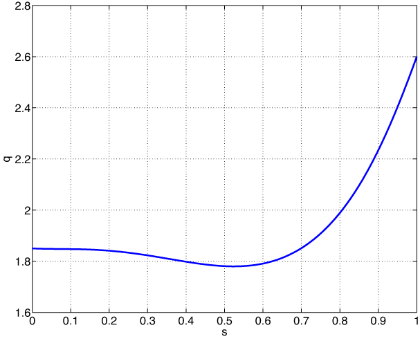
  $B_{0}=3.0~\text{T}$. Circular concentric flux surfaces are considered. The safety factor has a value of 1.85 at the axis, it decreases from $\unicode[STIX]{x1D70C}=0$ to $\unicode[STIX]{x1D70C}=0.5$, where the minimum value is located $(q(\unicode[STIX]{x1D70C}=0.5)=1.78)$, and then it rises to the edge, where it reaches the maximum value $(q(\unicode[STIX]{x1D70C}=1)=2.6)$ (see figure 1). Here, $\unicode[STIX]{x1D70C}$ is a normalized radial coordinate defined as $\unicode[STIX]{x1D70C}=r/a$.
Safety factor profile.
We choose a reference radial position of  $\unicode[STIX]{x1D70C}=\unicode[STIX]{x1D70C}_{r}=0.5$, corresponding to $s=0.525$, where the flux radial coordinate $s$ is defined as $s=\sqrt{\unicode[STIX]{x1D713}_{\text{pol}}/\unicode[STIX]{x1D713}_{\text{pol}}(\text{edge})}$, $\unicode[STIX]{x1D713}_{\text{pol}}$ being the poloidal magnetic flux. The ion and electron temperatures are taken to be equal: $T_{e}(\unicode[STIX]{x1D70C})=T_{i}(\unicode[STIX]{x1D70C})$. Here, differently from Biancalani et al. (Reference Biancalani, Bottino, Briguglio, Könies, Lauber, Mishchenko, Poli, Scott and Zonca2016), a value of $T_{e}(\unicode[STIX]{x1D70C}=\unicode[STIX]{x1D70C}_{r})$ corresponding $\unicode[STIX]{x1D70C}^{\ast }=\unicode[STIX]{x1D70C}_{s}/a=0.00571$, is chosen (with $\unicode[STIX]{x1D70C}_{s}=\sqrt{T_{e}/m_{i}}/\unicode[STIX]{x1D6FA}_{i}$ being the sound Larmor radius). The electron thermal to magnetic pressure ratio of $\unicode[STIX]{x1D6FD}_{e}=8\unicode[STIX]{x03C0}\langle n_{e}\rangle T_{e}(\unicode[STIX]{x1D70C}_{r})/B_{0}^{2}=5\times 10^{-4}$.
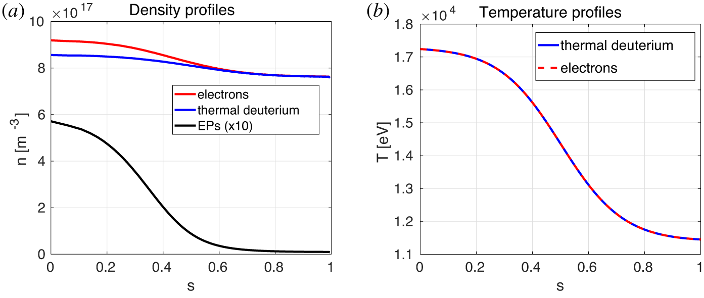
Density (a) and temperature (b) profiles, versus  $s$ radial coordinate, for $n_{EP}/n_{e}=0.01$.
We consider a deuterium plasma. This means that the chosen value of  $\unicode[STIX]{x1D70C}^{\ast }$ corresponds to a temperature at the reference position of $T_{e}(\unicode[STIX]{x1D70C}_{r})=14.05~\text{keV}$. This also corresponds to an average input electron density of $\langle n_{e}\rangle =0.795\times 10^{18}~\text{m}^{-3}$. Once the EP population is loaded into ORB5, we choose to satisfy the quasineutrality for the considered simulations. This means that ORB5 automatically re-calculates the electron density profile, in order to have $n_{EP}(\unicode[STIX]{x1D70C})+n_{i}=n_{e}(\unicode[STIX]{x1D70C})$ for all values of $\unicode[STIX]{x1D70C}$ (see figure 2). The thermal ion profile remains the same independently of the EP concentration. The thermal ion density on axis is $n_{i}(0)=0.870\times 10^{18}~\text{m}^{-3}$ and at the reference radius is $n_{i}(\unicode[STIX]{x1D70C}_{r})=0.818\times 10^{18}~\text{m}^{-3}$. Some characteristic frequencies and velocities can be calculated. The ion cyclotron frequency is $\unicode[STIX]{x1D6FA}_{i}=1.44\times 10^{8}~\text{rad}~\text{s}^{-1}$. The Alfvén velocity on axis is $v_{A}(0)=5.0\times 10^{7}~\text{m}~\text{s}^{-1}$. The sound velocity at the reference radius is $c_{s}(\unicode[STIX]{x1D70C}_{r})=\sqrt{T_{e}(\unicode[STIX]{x1D70C}_{r})/m_{i}}=8.21\times 10^{5}~\text{m}~\text{s}^{-1}$. The Alfvén frequency on axis is $\unicode[STIX]{x1D714}_{A}=v_{A}(0)/q(0)R_{0}=2.7\times 10^{6}~\text{rad}~\text{s}^{-1}=1.86\times 10^{-2}\,\unicode[STIX]{x1D6FA}_{i}$. The sound frequency at the reference radius is $\unicode[STIX]{x1D714}_{s}(\unicode[STIX]{x1D70C}_{r})=\sqrt{2}c_{s}(\unicode[STIX]{x1D70C}_{r})/R_{0}=1.16\times 10^{5}~\text{rad}~\text{s}^{-1}$.
The same analytical function is used for all the profiles of the equilibrium density and temperature, for the three species of interest (thermal deuterium, labelled here as ‘ $d$’, thermal electrons, labelled here as ‘ $e$’, and hot deuterium, labelled here as ‘ $EP$’). For the EP density, for example, the function is written as:
 $$\begin{eqnarray}n_{EP}(\unicode[STIX]{x1D70C})/n_{EP}(\unicode[STIX]{x1D70C}_{r})=\exp [-\unicode[STIX]{x0394}\,\unicode[STIX]{x1D705}_{n}\tanh ((\unicode[STIX]{x1D70C}-\unicode[STIX]{x1D70C}_{r})/\unicode[STIX]{x1D6E5})].\end{eqnarray}$$
 The value of  $\unicode[STIX]{x1D6E5}$ is the same for all species, for both density and temperature: $\unicode[STIX]{x1D6E5}=0.208$. Deuterium and electrons have $\unicode[STIX]{x1D705}_{n}=0.3$ and $\unicode[STIX]{x1D705}_{T}=1.0$, and the EP has $\unicode[STIX]{x1D705}_{n}=10.0$ and $\unicode[STIX]{x1D705}_{T}=0.0$ (i.e. the EPs have a flat temperature profile). Different values of the EP temperature are considered. The value of $\unicode[STIX]{x1D70C}_{r}$ is the reference radial position defined above.
The distribution function of the EP population is Maxwellian. The choice of the magnetic equilibrium, thermal plasma profiles and EP profiles and distribution function, is done for reasons of continuity with previous papers where results of AMs with ORB5 were presented (Biancalani et al. Reference Biancalani, Bottino, Briguglio, Könies, Lauber, Mishchenko, Poli, Scott and Zonca2016; Könies et al. Reference Könies, Briguglio, Gorelenkov, Fehér, Isaev, Lauber, Mishchenko, Spong, Todo and Cooper2018) as the main goal of this paper is to study the nonlinear dynamics of the electrons in a simplified case, where the effect is isolated and clearly visible. More experimentally accurate plasma configurations and distribution functions will be considered in the future, and discussed in dedicated papers. Different values of the EP averaged concentration  $\langle n_{EP}\rangle /n_{e}$ are considered.
In the nonlinear simulations shown in this paper, a Fourier filter in mode numbers is applied, keeping  $0\leqslant n\leqslant 9$ and $|m-nq(s)|\leqslant \unicode[STIX]{x1D6FF}_{m}$, with $\unicode[STIX]{x1D6FF}_{m}=3$ being the half-width of the band of poloidal modes. For the linear analysis, we additionally run simulations studying each separate toroidal mode number between $1$ and $9$. A convergence scan in $\unicode[STIX]{x1D6FF}_{m}$ has been performed going from $\unicode[STIX]{x1D6FF}_{m}=2$ to $\unicode[STIX]{x1D6FF}_{m}=10$. This scan shows that the results are near convergence already with a filter allowing only modes with $\unicode[STIX]{x1D6FF}_{m}=2$, in this regime. Regarding the radial direction, unicity boundary conditions are imposed to the potentials at the axis and Dirichlet at the external boundary. Here, by unicity boundary conditions, we mean Dirichlet boundary conditions (i.e. $\unicode[STIX]{x1D719}=0$ and $A_{\Vert }=0$) for all $m\neq 0$ and Neumann boundary conditions (i.e. $\unicode[STIX]{x2202}\unicode[STIX]{x1D719}/\unicode[STIX]{x2202}s=0$ and $\unicode[STIX]{x2202}A_{\Vert }/\unicode[STIX]{x2202}s=0$) for $m=0$. The value of the electron mass is chosen to be 200 times lighter than thermal ions. This value is proved to be at convergence (see appendix A).
4 Linear dynamics
In this section, we investigate the linear dynamics of AM in the equilibrium described in the previous section.
Dependence of the frequency (a) and growth rate (b) on the toroidal mode number  $n$. Here, $n_{EP}/n_{e}=0.01$ and $T_{EP}/T_{e}=10$. Modes below $n=5$ are stable.
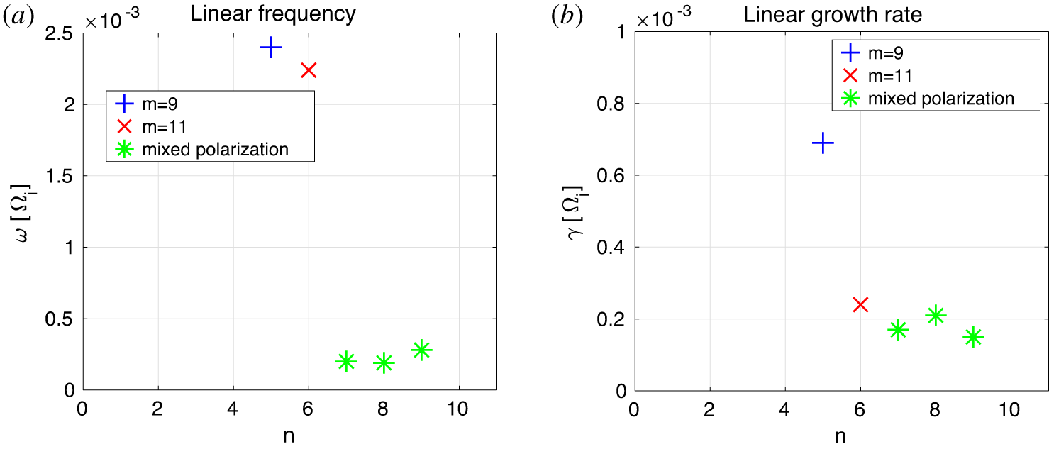
First, we perform a set of simulations, each of which keeps only one toroidal mode number, from  $n=1$ to $n=9$ (and a range of poloidal mode numbers $|m-nq(s)|\leqslant 3$), and measure the growth rate and the dominant polarization of the observed instabilities. The EP concentration and temperature are respectively $\langle n_{EP}\rangle /\langle n_{e}\rangle =0.01$ and $T_{EP}/T_{e}(\unicode[STIX]{x1D70C}_{r})=10$. The result is shown in figure 3. The most unstable mode is found at $n=5$, with a polarization in the poloidal direction of $m=9$. The second most unstable mode is $n=6$, with a polarization in the poloidal direction of $m=11$. These two modes are identified as Alfvénic instabilities, as their growth rate strongly depends on the EP concentration. Modes with higher toroidal mode number have a mixed $m$-polarization, typical of ion-temperature-gradient-driven modes (ITG) in electromagnetic simulations (Biancalani et al. Reference Biancalani, Bottino, Briguglio, Conway, Di Troia, Kleiber, Könies, Lauber, Mishchenko and Scott2014). Modes with toroidal mode number lower than $n=5$ are not found to grow in the considered time of the simulations. The frequency and growth rate of the most unstable mode, i.e. the mode with $n=5$, $m=9$, are
 $$\begin{eqnarray}\displaystyle & \displaystyle \unicode[STIX]{x1D714}_{\text{lin}}=2.4\times 10^{-3}\;\unicode[STIX]{x1D6FA}_{i}, & \displaystyle\end{eqnarray}$$
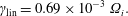 $$\begin{eqnarray}\displaystyle & \displaystyle \unicode[STIX]{x1D6FE}_{\text{lin}}=0.69\times 10^{-3}\;\unicode[STIX]{x1D6FA}_{i}. & \displaystyle\end{eqnarray}$$
 The identification of the Alfvén mode with  $n=5$, $m=9$ is performed in the standard way, described in the following. Firstly, we calculate the theoretical SAW continuous spectrum, for modes with $n=5$, for the magnetic equilibrium and the thermal plasma profiles given in § 3. The SAW continuous spectrum is the spectrum of the local solutions of the SAW dispersion relation. This is shown in figure 4(a). The formula is taken from Biancalani et al. (Reference Biancalani, Bottino, Briguglio, Könies, Lauber, Mishchenko, Poli, Scott and Zonca2016), where an approximation of small inverse aspect ratio $\unicode[STIX]{x1D716}$ is considered, slightly underestimating the width of the toroidal Alfvén eigenmode (TAE) gaps. This should be valid here, as $\unicode[STIX]{x1D716}$ is small. The points where the radial derivative of the continuum frequency vanishes are named continuum accumulation points (CAP). Modes living near the CAPs experience a negligible continuum damping, and are therefore more easily destabilized by an EP population (Grad Reference Grad1969; Chen & Hasegawa Reference Chen and Hasegawa1974; Chen & Zonca Reference Chen and Zonca2016). Two BAE CAPs are found: one at $s=0.39$, and one at $s=0.62$. The frequency of the BAE CAPs is calculated according to Zonca, Chen & Santoro (Reference Zonca, Chen and Santoro1996), Zonca & Chen (Reference Zonca and Chen2008), neglecting for simplicity the effects of the thermal density and temperature gradients. For reference, we note that the inner BAE CAP has a frequency of
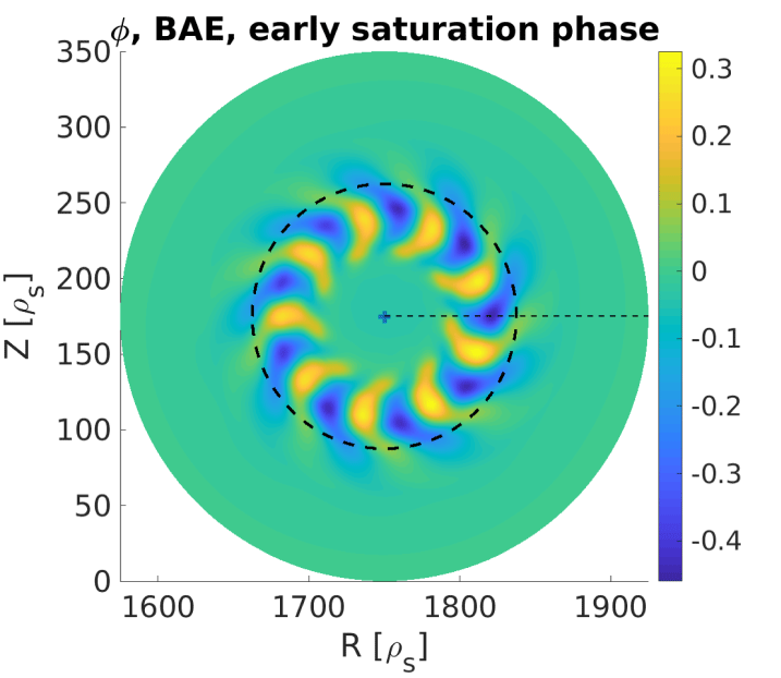
  $\unicode[STIX]{x1D714}_{\text{BAE}-\text{CAP}}=1.58\times 10^{-3}\,\unicode[STIX]{x1D6FA}_{i}$. Secondly, the spatial structure of the mode in the poloidal plane is investigated. A snapshot is given in figure 4(b). The mode is observed with clear poloidal polarization of $m=9$, and peaked at $s=0.39$. Thirdly, we make a scan of the frequency and growth rate as a function of the EP concentration. This is shown in figure 5. The mode frequency if found to tend to a frequency near the inner BAE CAP in the limit of $n_{EP}\rightarrow 0$. Note that the frequency is observed slightly above the BAE CAP for finite EP concentrations, analogously with what is described in Lauber (Reference Lauber2013). The marginal stability, due to the balance of the EP drive and the Landau damping, is found for $n_{EP}/n_{e}\simeq 10^{-3}$. Due to the spatial structure and to the frequency in relation to the SAW continuous spectrum, this mode is identified as the BAE at the inner continuum accumulation point. A further proof that this is an EP-driven mode is given by the characteristic ‘boomerang’ (or croissant) shape in the poloidal plane, i.e. the twisting radial mode structure (see for example Zhang et al. (Reference Zhang, Lin, Holod, Wang, Xiao and Zhang2010), Wang, Zonca & Chen (Reference Wang, Zonca and Chen2010), Ma, Zonca & Chen (Reference Ma, Zonca and Chen2015) for BAEs and Biancalani et al. (Reference Biancalani, Bottino, Briguglio, Könies, Lauber, Mishchenko, Poli, Scott and Zonca2016) for EPMs). This BAE is observed to rotate in the ion-diamagnetic direction.
(a) Theoretical SAW continuous spectrum for  $n=5$, depicting the position of the two BAE continuum accumulation points. (b) Poloidal structure of mode linearly excited with ORB5 with an EP population with $T_{EP}/T_{e}=10$. The black circular dashed line delimits the $s=0.5$ flux surface.

Dependence of the frequency (a) and growth rate (b) of BAEs with  $n=5$, $m=9$, on the EP concentration $n_{EP}$. Here, $T_{EP}/T_{e}=10$.
5 Description of the fully nonlinear simulation
In this section, we describe the nonlinear dynamics of the Alfvén modes in an equilibrium described in § 3. The analysis of the linear dynamics has been described in § 4, showing that a BAE with  $n=5$, $m=9$, is the most unstable mode. Here, we allow all modes with toroidal mode numbers in the interval $[0,9]$ to develop. For completeness, we report here that, in the case when only the $n=5$ mode is allowed to evolve, the nonlinear phase is found to be significantly different. The simulation is fully nonlinear, meaning that the markers for all species are pushed along perturbed trajectories. No Krook operator is applied here, meaning that there are no sources or sinks of energy due to the forcing of the profiles. A perturbation with $n=5$, $m=9$ is initialized at $t=0$. Unicity boundary conditions are applied at the axis, i.e. $s=0$, and Dirichlet at the edge, i.e. $s=1$.
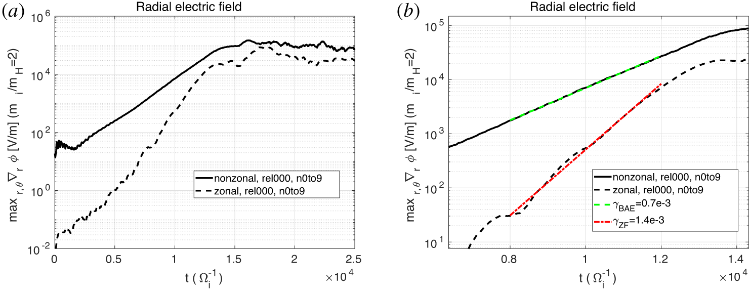
The zonal component of the radial electric field can be measured as the flux surface average of the total electric field at each radial position. The non-zonal component is defined as the difference of the total radial electric field and the zonal component, at each position in the poloidal plane ( $s$,
$s$,  $\unicode[STIX]{x1D703}$). The maximum values of these components are measured in the poloidal plane, at one given toroidal angle ( $\unicode[STIX]{x1D711}=0$), and at each time step, and their evolution in time is shown in figure 6(a). The non-zonal component describes the BAE field, whereas the zonal component describes the zonal flow. We note that there are 5 phases: (i) a first transient phase, where the BAE mode is forming ( $0<t<2000$, in $\unicode[STIX]{x1D6FA}_{i}^{-1}$ units); (ii) a linear phase, where the BAE grows linearly but the ZF is still at noise levels $(2000<t<7000)$; (iii) an early nonlinear phase, where the BAE continues growing exponentially, but the ZF starts growing in amplitude with higher growth rate, meaning that a nonlinear coupling is already occurring $(7000<t<13\,000)$; (iv) an early saturation phase, where the BAE instantaneous growth rate starts decreasing, with respect to the linear value $(13\,000<t<16\,000)$; (v) a deep saturated phase, after the BAE field has reached the maximum level of $\unicode[STIX]{x1D6FF}\tilde{E}_{r}\simeq 1.0e5~\text{V}~\text{m}^{-1}$, and starts decreasing in amplitude $(t>16\,000)$. In this paper, we focus on the dynamics of the BAE and ZF in the early nonlinear phase and early saturation phase $(7000<t<16\,000)$.
The investigation of the early nonlinear phase shows that the ZF starts growing with a growth rate of  $\unicode[STIX]{x1D6FE}_{ZF}=1.4e-3\unicode[STIX]{x1D6FA}_{i}$, i.e. double of the BAE linear growth rate. This is a signature of the mechanism named forced-driven excitation, observed numerically with MEGA (Todo et al. Reference Todo, Berk and Breizman2010) and GTC (Zhang & Lin Reference Zhang and Lin2013) and explained analytically in Qiu et al. (Reference Qiu, Chen and Zonca2016).
(a) Evolution of the non-zonal (continuous) and zonal (dashed) components of the radial electric field. (b) Zoom in of the early nonlinear phase.
BAE spatial structure at  $t=15\,000$.
The spatial structure of the BAE is observed to change during the early saturation phase. In particular, the radial width becomes larger and the ‘arms’ of the ‘boomerang’ extend towards the axis and the second BAE CAP (see figure 7). This is a signature of a weaker interaction of the eigenmode with the continuum occurring during the early nonlinear saturation phase, with respect to the early nonlinear phase, consistently with Biancalani et al. (Reference Biancalani, Bottino, Cole, Di Troia, Lauber, Mishchenko, Scott and Zonca2017). Incidentally, we note that the main dynamics of the BAE and of the ZF is not found to significantly change if the simulations are run with a flat temperature profile, meaning that the global properties of the temperature profiles are not substantial for the analysis of the modes considered here. On the other hand, the saturation level of the BAE is found to be different, namely lower, if we filter the ZF, namely the  $n=0$ component, out, i.e. if we perform a simulation keeping only the modes with $1\leqslant n\leqslant 9$. This means that, for a correct prediction of the saturation levels of AMs, the nonlinear coupling to the ZFs should be retained. Simulations with a broader range of toroidal mode numbers (up to $0\leqslant n\leqslant 40$) do not show a different BAE saturation level, in this regime. This proves that the range chosen in this paper ( $0\leqslant n\leqslant 9$) is sufficient for the present study. We have also run simulations with drift-kinetic thermal ions, instead of GK thermal ions. The result in the saturation level does not substantially change, and the simulation takes approximately 20 % less computational time. Nevertheless, note that GK ions are necessary in the view of studying the interaction of AMs and ITGs (which is the continuation of the present paper).
6 Contribution of the different species to the nonlinear dynamics
During the linear excitation phase, Alfvén modes tap the free energy stored in the EP profile. This role of the EP population is well known and it has been studied extensively in the literature, as mentioned in the Introduction. In general, the two ways energy can be exchanged between waves and particles of a given species  $s$, are described via non-uniformities in velocity or real space (see, for example, Betti & Freidberg Reference Betti and Freidberg1992). The corresponding contributions to the growth rate have the following dependencies on the distribution function $F_{s}$ of the species:
 $$\begin{eqnarray}\displaystyle & \displaystyle \unicode[STIX]{x1D6FE}_{\unicode[STIX]{x1D716}}\propto \unicode[STIX]{x1D714}\frac{\unicode[STIX]{x2202}F_{s}}{\unicode[STIX]{x2202}\unicode[STIX]{x1D716}}, & \displaystyle\end{eqnarray}$$
 $$\begin{eqnarray}\displaystyle & \displaystyle \unicode[STIX]{x1D6FE}_{\unicode[STIX]{x1D713}}\propto -\frac{n}{q_{s}}\frac{\unicode[STIX]{x2202}F_{s}}{\unicode[STIX]{x2202}\unicode[STIX]{x1D713}}, & \displaystyle\end{eqnarray}$$
 where  $\unicode[STIX]{x1D716}$ is the particle energy, $\unicode[STIX]{x1D713}$ is the flux coordinate and $q_{s}$ is the charge of the species $s$. In the case of energetic ions, equation (6.2) shows that a negative radial gradient of the density yields a drive.
(a) EP profiles depicted at4 selected times in the early nonlinear phase and early saturation phase. (b) The corresponding perturbed relative EP density.
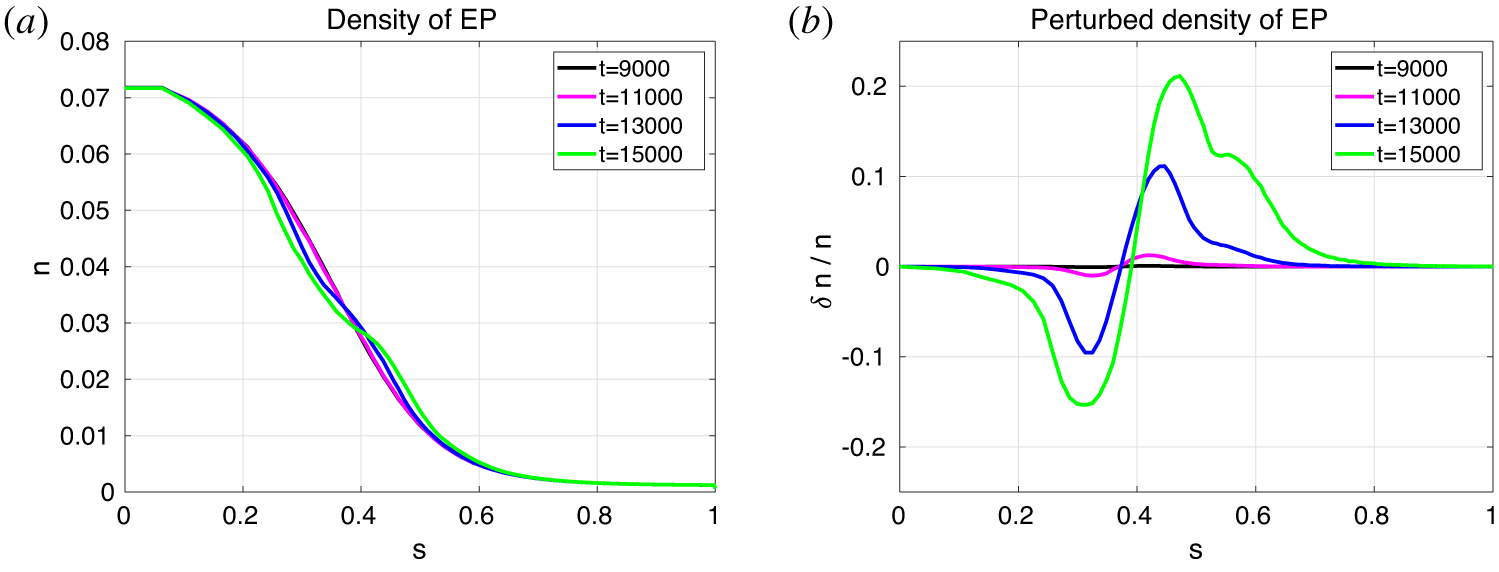
During the early saturation phase, the EP population is redistributed radially in the outward direction. This phenomenon can be observed also for the BAE observed in the simulations considered in this paper. In figure 8, the outward redistribution of the EP population is shown, around the peak position of the BAE,  $s=0.39$. In figure 8(b), note that the characteristic ‘hole’ structure forms near the BAE peak, on the side where the EP profile is depleted, whereas the ‘clump’ structure forms near the BAE peak, on the side where the EP density increases.
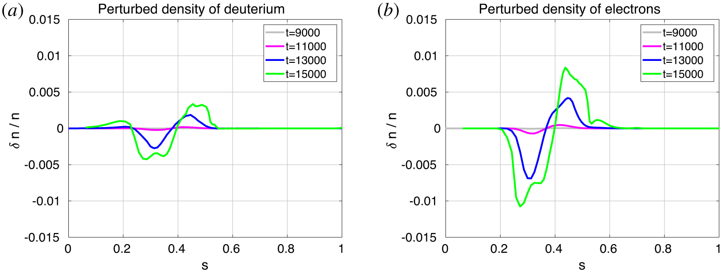
Perturbed relative density of the thermal ions (a) and electrons (b).
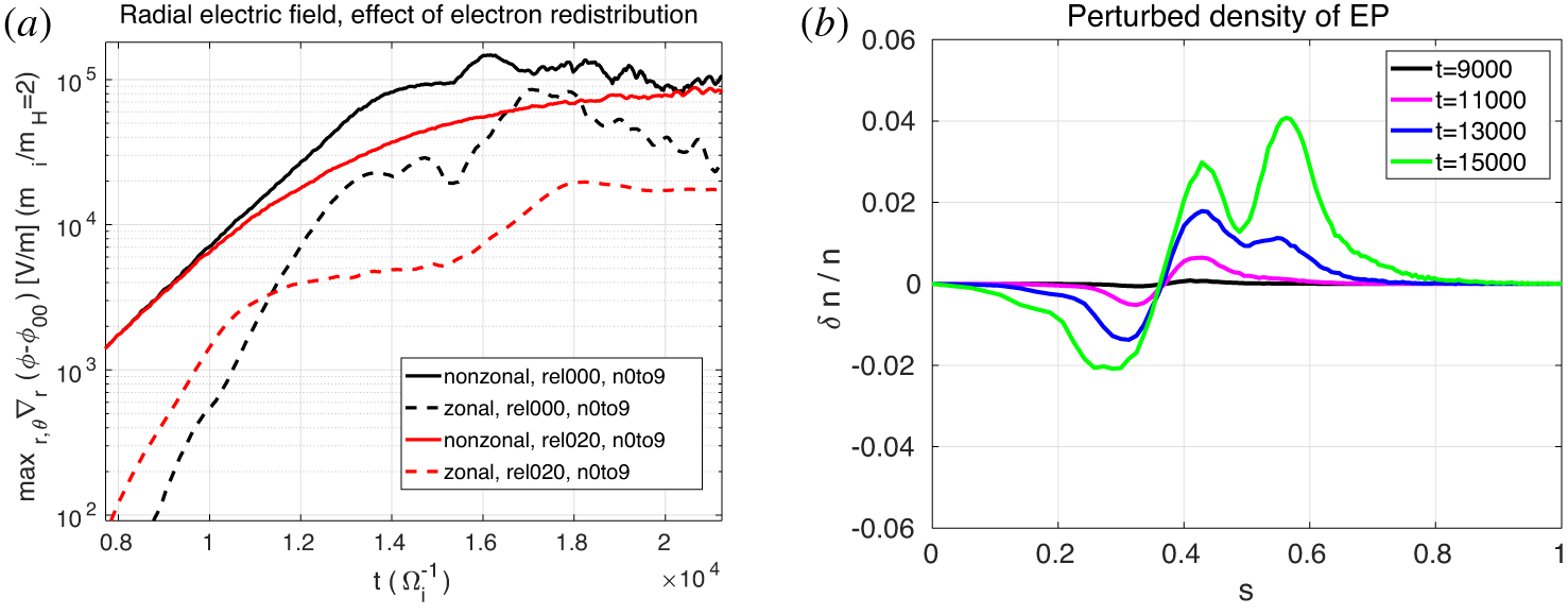
(a) Evolution in time of the radial electric field non-zonal and zonal components for the fully nonlinear simulation (black lines, also depicted in figure 6) and for a simulation where the electrons are not allowed to redistribute (red lines). (b) EP perturbed density for the simulation where the electrons are not allowed to redistribute.
On the other hand, the role of the redistribution of the thermal species, in the saturation of Alfvén modes, has been less investigated in the literature. As an example, we now repeat the same study of the perturbed radial density profile done for the EP, for the thermal ions (in our case, deuterium) and electrons. The result is shown in figure 9. As for the EP, two clear hole and clump structures are observed for the ion and electron species, as well. The positions of the hole and the clump are the same as for the EP population, denoting the resonance radial location and BAE radial width. Note that the radial extent of the perturbed densities is the same for the ions and electrons, ensuring quasineutrality.
The thermal ion relative perturbed density is observed to be significantly smaller than for the electrons, and its effect is also less important, as discussed later. On the other hand, the electron perturbed density is not negligible and a strong effect of the electron kinetic dynamics on the nonlinear evolution of the mode is observed in the simulations. Note that the hole and clump observed in the electron perturbed density, corresponding to a flattening of the electron profile, reflect a decreased damping, instead of a decreased drive, which was the case of the EP. This is due to the different charge of the electrons with respect to the EP, i.e. the energetic deuterium in the case considered here (see (6.2)). Note also that, in general, both terms described by (6.1) and (6.2) are important and each of them can be the dominant one, in different regimes. In figure 9, the term described in (6.2) is shown as an example.
In order to check the relevance of the electron redistribution for the nonlinear dynamics of the BAE, we perform a simulation where the electrons are pushed along the unperturbed trajectories. This means that, although the thermal and energetic ions are still allowed to redistribute, the electrons are forced to remain in the initial profile. The result can be observed in figure 10(a). We observe that, in the simulation where the electrons are not allowed to redistribute, the early saturation phase starts earlier, namely at  $t=9000$ instead of $t=13\,000$, and the BAE amplitude grows more slowly. The cause is a stronger damping due to the electrons. The effect is that, at a given time, the EP redistribution is much lower than in the fully nonlinear case. This is shown in figure 10(b).
A simulation with electrons and EPs pushed along perturbed trajectories and thermal ions pushed along unperturbed trajectories has also been performed, and no significant difference has been found with respect to the fully nonlinear case. This proves that the nonlinear kinetic dynamics of the ions is not relevant in this regime.
Level of the zonal electric field measured around the time of the BAE saturation, for simulations where only EPs are allowed to redistribute nonlinearly (blue line), and for fully nonlinear simulations, i.e. where all species are allowed to redistribute (red line).
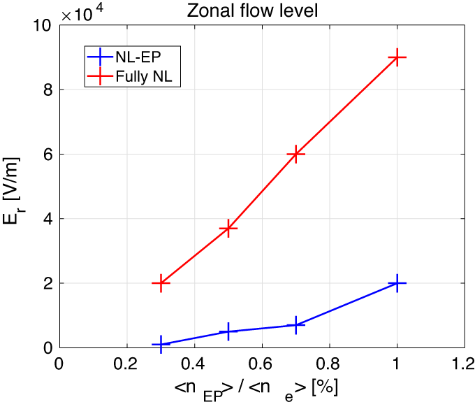
Finally, we want to investigate how the electron redistribution affects the excitation of zonal structures. In figure 10, the evolution in time of the zonal radial electric field is shown for the fully nonlinear case (labelled ‘rel000’), and for the case where the electrons are not allowed to redistribute (labelled ‘rel020’). The zonal radial electric field is found to reach significantly higher values in the fully nonlinear case. The reason is the zonal flow is found to follow the analytical prediction of the forced-driven excitation, with double growth rate with respect to the BAE, only during the early nonlinear phase. In the simulation where the electrons are not allowed to redistribute, the early saturation phase starts earlier, and the zonal flow growth rate drops to small values earlier, leaving the ZF at lower levels. This is not a threshold effect, but it increases linearly with the EP drive (see figure 11).
We also note that the growth rate of the ZF during the early nonlinear phase is twice that of the BAE, even in simulations where either one or both the thermal species are not allowed to redistribute. This confirms that, in the early nonlinear phase, the forced-driven excitation is mediated dominantly by the nonlinearity associated with the EPs, as predicted in Qiu et al. (Reference Qiu, Chen and Zonca2016). The main result described in this paper is that the situation changes in the early saturation phase, where the nonlinearity associated with the thermal species, and especially with the electrons, becomes important.
7 Conclusions
Alfvén modes are present in tokamak plasmas heated by energetic particles and they are expected in future fusion devices. Due to their strong nonlinear interaction with the EP population, they are considered with great attention in the theoretical models which aim at being comprehensive. In particular, understanding the saturation level of Alfvén modes in present tokamak plasmas, and predicting it in future fusion devices, is one of the main tasks of the present theoretical community.
The main focus of the analytical and numerical investigation of AMs of the past decades has been the nonlinear wave–particle interaction of AMs and EPs. This has been considered as the main saturation mechanism of AMs. Here, we extend this focus to the wave–particle interaction of AMs with the thermal species, which has been neglected in the past. The profiles of thermal ions and electrons are allowed to redistribute.
For simplicity, a magnetic configuration with circular flux surfaces and large aspect ratio is considered. The beta-induced Alfvén eigenmode is observed to be linearly unstable in this configuration, and its linear and nonlinear evolution is studied in simulations where all modes from toroidal mode number  $n=0$ to $n=9$ are included. The inclusion of the axisymmetric mode $n=0$ allows us to investigate as well the excitation of zonal flows. The evolution of the BAE is found to be different in simulations where only one toroidal mode is allowed to evolve.
This numerical investigation is performed with the global gyrokinetic particle-in-cell code ORB5. ORB5 was written for turbulence studies, and therefore a sensible effort was put in building a model containing a self-consistently nonlinear set of equations. The extension of ORB5 to its present electromagnetic multi-species version, allows us to investigate global electromagnetic modes like low- $n$ AMs. The gyrokinetic framework, on the other hand, allows us to have all the main kinetic effects, for all species, automatically included in the AM dynamics.
The result of this investigation, is that the BAE saturation occurs primarily due to the profile relaxation of all the species. Although the EP profile relaxation is confirmed to play a central role in the saturation, by decreasing the drive in the nonlinear phase, nevertheless, the nonlinear kinetic dynamics of the thermal species, and in particular of the electrons, cannot be neglected if one wants to correctly estimate the saturation level of the BAE and of the forced-driven ZF. Although the ions give a small contribution, nevertheless the electrons strongly affect the nonlinear dynamics due to their damping, which relaxes in time when their profile radially redistributes.
In summary, the contribution of the electron redistribution to the nonlinear saturation of BAEs and consequent excitation of ZFs is proven here to be important in explaining the higher saturation levels of BAEs and ZFs observed in fully nonlinear simulations, with respect to simulations where only the wave–particle nonlinearity with the EPs is considered. This result indicates that, in general, the nonlinear kinetic dynamics of electrons should not be neglected, if one wants to have correct predictions of the Alfvén mode saturation levels and zonal flows amplitudes.
As future steps, the dynamics of the different species in real space (including the poloidal direction) and in phase space (to locate the resonances and quantify the power spectrum) will be investigated more in detail. Moreover, the importance of the electron damping in fully nonlinear simulations will be studied in more experimentally relevant magnetic configurations, and compared with the experimental measurements. The investigation of the interaction of BAEs with higher- $n$ modes like ITG modes is in progress.
Acknowledgements
Interesting discussions with F. Zonca, Z. Qiu, L. Villard, F. Jenko, I. Novikau and A. Di Siena are gratefully acknowledged. This work has been carried out within the framework of the EUROfusion Consortium and has received funding from the Euratom research and training program 2014–2018 and 2019–2020 under grant agreement no 633053 within the framework of the Multiscale Energetic particle Transport (MET) European Eurofusion Project. The views and opinions expressed herein do not necessarily reflect those of the European Commission. Simulations were performed on the HPC-Marconi supercomputer within the framework of the ORBFAST and OrbZONE projects.
Editor Francesco Califano thanks the referees for their advice in evaluating this article.
Appendix A. Convergence with the electron mass
Here, we show the convergence scan with the mass ratio, for simulations with  $\langle n_{EP}\rangle /\langle n_{e}\rangle =0.03$. In figure 12 we can see that going from $m_{i}/m_{e}=100$ to $m_{i}/m_{e}=200$ we still see some slight difference in the linear growth rates, which becomes even smaller from $m_{i}/m_{e}=200$ to $m_{i}/m_{e}=400$. The saturation levels, on the other hand, seem unchanged. Therefore, convergence is achieved.
Non-zonal (continuous lines) and zonal (dashed lines) radial electric field. rel000 denotes fully nonlinear simulations. rel020 denotes simulations where the electrons are pushed along unperturbed trajectories. Note that the convergence on the mass ratio is achieved.


 Open access