







1. Introduction
Turbulent flows that are constrained by a wall (referred to as ‘wall turbulence’) are common in nature and technology. Roughly half of the energy spent in transporting fluids through pipes or vehicles through air or water is dissipated by the turbulence near the walls (Jiménez Reference Jiménez2012). Therefore, an improved understanding of the underlying physics of these flows is essential for modelling and control (Kim Reference Kim2011; Canton et al. Reference Canton, Örlü, Chin, Hutchins, Monty and Schlatter2016; Yao, Chen & Hussain Reference Yao, Chen and Hussain2018). The spatially evolving boundary layer, the (plane) channel and the pipe are three canonical geometrical configurations of wall turbulence. Different from boundary layer and channel flows, azimuthal periodicity is inherent to pipe flows. Therefore, pipe flow is the most canonical case, being completely described by the Reynolds number ( $Re$) and the axial length – the effect of the latter is limited if sufficiently large (El Khoury et al. Reference El Khoury, Schlatter, Noorani, Fischer, Brethouwer and Johansson2013; Feldmann, Bauer & Wagner Reference Feldmann, Bauer and Wagner2018).
Sustained interest in high- $Re$ wall turbulence stems from numerous open questions regarding the scaling of turbulent statistics, as reviewed in Marusic et al. (Reference Marusic, McKeon, Monkewitz, Nagib, Smits and Sreenivasan2010b) and Smits, McKeon & Marusic (Reference Smits, McKeon and Marusic2011b). For example, a characteristic of high- $Re$ wall turbulence is the logarithmic law in the mean velocity with an important parameter, namely the von Kármán constant $\kappa$, whose value and universality among different flow geometries are still highly debated (Nagib & Chauhan Reference Nagib and Chauhan2008; She, Chen & Hussain Reference She, Chen and Hussain2017). Also, there is no consensus on whether the near-wall peak of the streamwise velocity fluctuations increases continuously with $Re$ (Marusic, Baars & Hutchins Reference Marusic, Baars and Hutchins2017) or eventually saturates at high $Re$ (Chen & Sreenivasan Reference Chen and Sreenivasan2021; Klewicki Reference Klewicki2022). Furthermore, the existence of an outer peak in the streamwise velocity fluctuations, as indicated by experiments, is also highly debated (Hultmark et al. Reference Hultmark, Vallikivi, Bailey and Smits2012; Willert et al. Reference Willert, Soria, Stanislas, Klinner, Amili, Eisfelder, Cuvier, Bellani, Fiorini and Talamelli2017). Other questions, which can be answered only with substantially higher $Re$ values, concern the scaling and generation mechanism of the various flow structures. Large-scale motions (LSMs) and very-large-scale motions (VLSMs), with lengths $5R$ up to $20R$, have been found experimentally in the outer region of pipe flows (Kim & Adrian Reference Kim and Adrian1999; Monty et al. Reference Monty, Stewart, Williams and Chong2007). Here, $R$ is the radius of the pipe. Due to the increasing strength of these structures with $Re$, they have a footprint quite close to the wall (Monty et al. Reference Monty, Stewart, Williams and Chong2007), in the form of amplitude modulation as reviewed by e.g. Dogan et al. (Reference Dogan, Örlü, Gatti, Vinuesa and Schlatter2018).
Fundamental studies of wall turbulence require accurate representations or measurements of the flows, which were typically carried out via experiments (Zagarola & Smits Reference Zagarola and Smits1998; McKeon, Zagarola & Smits Reference McKeon, Zagarola and Smits2005; Smits et al. Reference Smits, Monty, Hultmark, Bailey, Hutchins and Marusic2011a; Furuichi et al. Reference Furuichi, Terao, Wada and Tsuji2015, Reference Furuichi, Terao, Wada and Tsuji2018; Talamelli et al. Reference Talamelli, Persiani, Fransson, Alfredsson, Johansson, Nagib, Rüedi, Sreenivasan and Monkewitz2009; Fiorini Reference Fiorini2017). However, decades of experimental research have shown that obtaining unambiguous high- $Re$ data, particularly near the wall, remains a challenge. This is because the smallest scales decrease with increasing $Re$ – leading to large uncertainties in determining the probe locations and turbulence intensities. Advances in computer technology (in both hardware and software) have enshrined direct numerical simulations (DNS) as an essential tool for turbulence research. Although only moderate $Re$ can be achieved at the current stage, DNS provide extensive, detailed data compared to experiments – even close to the walls where experimental data are very difficult to obtain. One of the earliest DNS for wall turbulence were performed by Kim, Moin & Moser (Reference Kim, Moin and Moser1987) for the channel flow at friction Reynolds number $Re_\tau \ (\equiv u_\tau h/\nu )\approx 180$ (here, $u_\tau$ is the friction velocity, $h$ is the half-channel height, and $\nu$ is the fluid kinematic viscosity). They found good agreement between DNS and experimental data of Hussain & Reynolds (Reference Hussain and Reynolds1975), except in the near-wall region. The discrepancy was speculated to be caused by the inherent near-wall hot-wire measurement errors. Eggels et al. (Reference Eggels, Unger, Weiss, Westerweel, Adrian, Friedrich and Nieuwstadt1994) subsequently conducted the first DNS of pipe flow at $Re_\tau \approx 180$ to investigate the differences between channel and pipe flows.
Numerous DNS investigations have been carried out in the aftermath of these pioneering studies, with  $Re$ increasing progressively as a result of increased computational power (Moser, Kim & Mansour Reference Moser, Kim and Mansour1999; Wu & Moin Reference Wu and Moin2008; Bernardini, Pirozzoli & Orlandi Reference Bernardini, Pirozzoli and Orlandi2014). However, among them, only those with $Re_\tau \ge 10^3$ are of particular engineering interest as this is the range of $Re$ relevant to industrial applications. Also, it is in this range that the high- $Re$ characteristics of wall turbulence start to manifest. One of the highest $Re_\tau$ large-domain DNS was performed by Lee & Moser (Reference Lee and Moser2015) for channel flows at $Re_\tau = 5186$ with domain size $L_x\times L_z=8{\rm \pi} h\times 3{\rm \pi} h$. Compared to numerous DNS for channel flows (Bernardini et al. Reference Bernardini, Pirozzoli and Orlandi2014; Lozano-Durán & Jiménez Reference Lozano-Durán and Jiménez2014; Lee & Moser Reference Lee and Moser2015), fewer high- $Re$ studies have addressed pipe flow, and most of them are limited to $Re_\tau \approx 1000$. For example, Lee & Sung (Reference Lee and Sung2013) performed DNS at $Re_\tau \approx 1000$ with length $30R$ and established the existence of VLSMs of scale up to ${O}(20R)$. El Khoury et al. (Reference El Khoury, Schlatter, Noorani, Fischer, Brethouwer and Johansson2013) used a spectral-element method to perform DNS for $Re_\tau$ up to 1000 with length $L_z=25R$. Chin, Monty & Ooi (Reference Chin, Monty and Ooi2014) found that the mean velocity profile does not exhibit a strictly logarithmic layer with $Re_\tau$ up to 2000, necessitating a finite- $Re$ correction like those introduced by Afzal (Reference Afzal1976) and Jiménez & Moser (Reference Jiménez and Moser2007). To quantify the effects of computational length and $Re$, Feldmann et al. (Reference Feldmann, Bauer and Wagner2018) conducted DNS for $90\le Re_\tau \le 1500$ with $L_z$ up to $42R$. They confirmed that $L_z=42R$ is sufficiently large to capture the LSM- and VLSM-relevant scales. Ahn et al. (Reference Ahn, Lee, Lee, Kang and Sung2015) performed DNS of pipe flow at $Re_\tau \approx 3000$ for length $30R$. They claimed that the mean velocity follows a power law in the overlap region, and observed a clear scale separation between inner- and outer-scale turbulence. So far, the largest DNS of pipe flow have been done at $Re_\tau \approx 6000$ with a relatively short length ( $L_z=15R$) by Pirozzoli et al. (Reference Pirozzoli, Romero, Fatica, Verzicco and Orlandi2021) based on a lower-order numerical method.
In general, one expects various simulations and experiments to agree with each other to a high degree. However, a comparison among several datasets in spatially developing turbulent boundary layers (Schlatter & Örlü Reference Schlatter and Örlü2010), channels (Lee & Moser Reference Lee and Moser2015) and pipes (Pirozzoli et al. Reference Pirozzoli, Romero, Fatica, Verzicco and Orlandi2021) shows, surprisingly, considerable variations among the various DNS, even for basic measures such as the shape factor, the friction coefficient and the von Kármán constant. Accurate turbulence statistics are very much needed, both for understanding turbulence physics and for developing, adapting and validating turbulence models. Here, we present a new high-fidelity DNS dataset of turbulent pipe flow generated with a pseudo-spectral method for  $Re_\tau$ up to $5200$ and with axial length $L_z/R=10{\rm \pi}$, which is long enough to capture the LSMs and VLSMs reported in experimental studies (Guala, Hommema & Adrian Reference Guala, Hommema and Adrian2006). The accuracy of this dataset is quantified by using the newly developed uncertainty quantification method. In addition, the dataset is compared extensively with other DNS and experimental data for turbulent pipe and channel flows.
2. Simulation details
DNS of incompressible turbulent pipe flows are performed using the pseudo-spectral code ‘OPENPIPEFLOW’ developed by Willis (Reference Willis2017). The radial, axial and azimuthal directions are represented by  $r$,
$r$,  $z$ and $\theta$, and the corresponding velocity components are $u_r$, $u_z$ and $u_\theta$. In the periodic axial ( $z$) and azimuthal ( $\theta$) directions, Fourier discretization is employed, and the numbers of Fourier modes in the $z$- and $\theta$-directions are $N_z$ and $N_\theta$, respectively. Note that in the physical space, the numbers of grid points in the $z$- and $\theta$-directions increase by a factor $3/2$ due to dealiasing. In the radial ( $r$) direction, a central finite difference scheme with a nine-point stencil is adopted. With this, the first- and second-order derivatives are, respectively, calculated to 8th and 7th order, which is reduced while approaching the boundaries. The grid points are distributed according to a hyperbolic tangent function so that high wall-normal velocity gradients in the viscous sublayer can be resolved. In addition, the first few points near $r = 0$ are also clustered to preserve the high order of the finite difference scheme across the pipe axis. No-slip and no-penetration boundary conditions are enforced at the wall (i.e. $r/R=1$), where an actual grid point is located. To avoid numerical singularity, there is no grid point at $r = 0$; and the boundary conditions on the extrapolated fields are specified based on symmetry. In particular, given a Fourier mode with azimuthal index $m$, each mode is odd/even if $m$ is odd/even for $u_z$ and $p$, and each mode is even/odd if $m$ is odd/even for $u_r$ and $u_\theta$. The governing equations are integrated with a second-order semi-implicit time-stepping scheme. The flow is driven by a pressure gradient, which varies in time to ensure that the mass flux through the pipe remains constant. For more details about the code and the numerical methods, see Willis (Reference Willis2017).
Five different Reynolds numbers,  $Re_\tau \approx 180$, $550$, $1000$, $2000$, and $5200$, are considered. The detailed simulation parameters, such as domain sizes and grid sizes, are listed in table 1. The simulations are performed with resolutions comparable to those used in the prior simulations, e.g. Lozano-Durán & Jiménez (Reference Lozano-Durán and Jiménez2014) and Lee & Moser (Reference Lee and Moser2015). In particular, for $Re_\tau \le 2000$, the axial and azimuthal resolutions employed here satisfy the criterion suggested by Yang et al. (Reference Yang, Hong, Lee and Huang2021) for capturing $99\,\%$ of the wall shear stress events. For the highest $Re_\tau$ case (i.e. $\approx 5200$), $N_z=12\,288$ and $N_\theta =5120$ Fourier modes are used in the $z$- and $\theta$-directions – corresponding to an effective resolution $\Delta z^+=L^+_x/N_z=12.8$ and $\Delta (R\theta )^+=(2{\rm \pi} R^+)/N_\theta =5.1$. Hereinafter, the superscript $+$ indicates non-dimensionalization in wall units, i.e. with kinematic viscosity $\nu$ and friction velocity $u_\tau$. Along the radial direction, the minimum and maximum grid spacings in wall units are $0.2$ and $8.6$, respectively. Additional information on this highest $Re_\tau$ simulation is provided in Appendix A.
Summary of simulation parameters. The axial length of the pipe ( $L_z$) is $10{\rm \pi} R$, with $R$ being the pipe radius. Here, $Re_\tau (\equiv u_\tau R/\nu )$ and $Re_b (\equiv 2U_b R/\nu )$ are the frictional and bulk Reynolds numbers, respectively; $N_z$ and $N_\theta$ are the number of dealiased Fourier modes in the axial and azimuthal directions, and $N_r$ is the number of grid points in the radial direction; $\Delta z$ and $\Delta (R\theta )$ are the grid spacings in the axial and azimuthal directions, defined in terms of the Fourier modes. In the radial direction, $\Delta r^+_w$ represents the grid spacing at the wall, and $\Delta r^+_{max}$ denotes the maximum grid spacing. Also, $T u_\tau /R$ is the total eddy-turnover time without the initial transient phase.

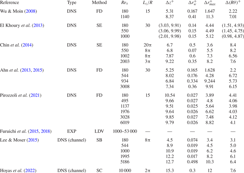
For comparison, several DNS and experimental data from the literature are included. The details are listed in table 2. To further validate the accuracy of our simulation, an additional simulation at  $Re_\tau =2000$ is performed using NEK5000 (hereinafter, this case is denoted as NEK5000 2K). The numerical set-up and mesh generation are the same as those in El Khoury et al. (Reference El Khoury, Schlatter, Noorani, Fischer, Brethouwer and Johansson2013). The length of the pipe is chosen as $L_z=35R$, and the total number of spectral elements is $7\,598\,080$. With the polynomial order set to $12$, the total number of grid points is approximately $13.1\times 10^9$. The grid spacing is comparable to that used in El Khoury et al. (Reference El Khoury, Schlatter, Noorani, Fischer, Brethouwer and Johansson2013) in all directions.
List of references of data used. FD denotes (second order) finite difference, SE denotes spectral element, SB denotes spectral/B-spline, SC denotes spectral/compact finite difference, and LDV represents laser Doppler velocimetry.  $L_z$ is the axial (streamwise) length, $\Delta z$ and $\Delta (R\theta )$ are the grid spacing in the axial and azimuthal directions, defined in terms of the Fourier modes. In the radial direction, $\Delta r^+_w$ represents the grid spacing at the wall, and $\Delta r^+_{max}$ denotes the maximum grid spacing.
The uncertainty in the flow quantities due to the finite time-averaging is estimated using the methods described in Rezaeiravesh et al. (Reference Rezaeiravesh, Xavier, Vinuesa, Yao, Hussain and Schlatter2022) and D. Xavier et al. (personal communication 2022). For the central moments of velocity and pressure, the central limit theorem is applied to the time samples averaged over the  $z$- and $\theta$-directions. The associated time-averaging uncertainty is estimated using an autoregressive-based model for the autocorrelation function; see e.g. Oliver et al. (Reference Oliver, Malaya, Ulerich and Moser2014). For estimating the uncertainty in the combination of central moments, the method proposed by Rezaeiravesh et al. (Reference Rezaeiravesh, Xavier, Vinuesa, Yao, Hussain and Schlatter2022) is employed. See Appendix B for further discussion on the method and estimated uncertainties in the first- and second-order velocity moments. For the $Re_\tau\approx 5200$ case, the estimated standard deviation of the mean axial velocity ( $U^+$) is less than 0.1 %, and the estimated standard deviation of the velocity variance (i.e. $\langle{u'^2_r}\rangle^{+}$, $\langle{u'^2_\theta}\rangle^{+}$, $\langle{u'^2_z}\rangle^{+}$) and covariance ( $\langle{u'_ru'_z}\rangle^{+}$) is less than 1 % in the near-wall region ( $y^+ < 100$), and approximately 5 % in the core region. Hereinafter, the velocity fluctuations are denoted using the prime symbol (e.g. $u'_r$), and the ensemble (in both time and space) averaged quantities are expressed using a capital letter or bracket (e.g. $U$ or $\langle{u'_r u'_\theta}\rangle$).
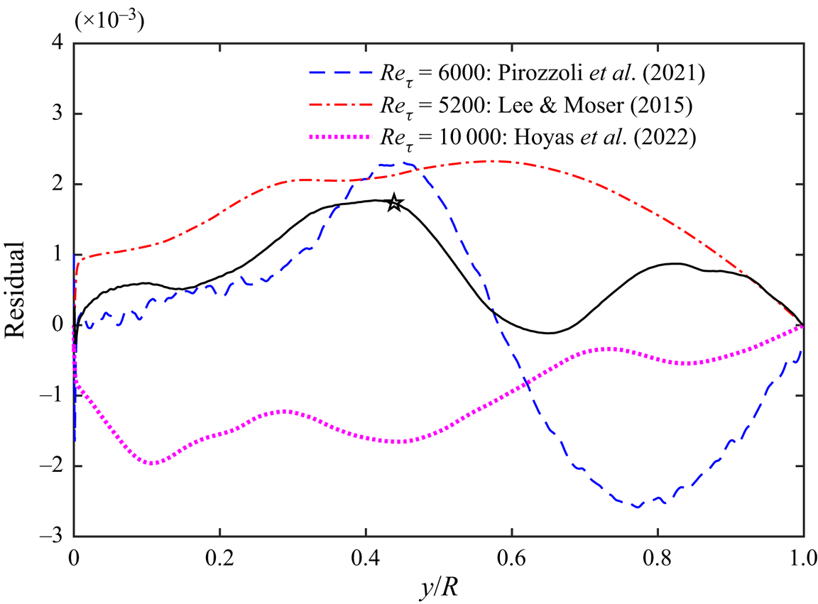
In addition, the mean momentum equation is employed to ensure that the simulation is statistically stationary. Due to momentum balance, the total stress, which is the sum of Reynolds shear stress  $\langle{u'_ru'_\theta }\rangle^{+}$ and mean viscous stress $\partial U^+/\partial y^+$, is linear in a statistically stationary turbulent pipe flow:
 \begin{equation} \frac{\partial U^+}{\partial y^+}-\langle{u'_ru'_\theta}\rangle^+{=}1-y/R, \end{equation}
where  $y=R-r$. Figure 1 shows the residual in (2.1) for the $Re_\tau \approx 5200$ case. The discrepancy between the analytic linear profile (i.e. $1-y/R$) and total stress profile (i.e. $\partial U^+/\partial y-\langle{u'_ru'_\theta }\rangle^{+}$) from the simulation is less than 0.002 in wall units and is comparable to other high- $Re$ DNS in the literature. Note that this discrepancy is much smaller than the standard deviation of the estimated total stress (see Appendix B).
Comparison of the residual in the mean momentum equation (2.1) among different high- $Re$ simulations. The black solid line with a star denotes our $Re_\tau =5200$ result.
3. Results
3.1. Flow visualization
The  $Re$ effect on the flow structure is illustrated qualitatively in figure 2, showing cross-sectional views of the instantaneous axial velocity $u_z$. Although large scales dominate in the central region of the pipe for all $Re_\tau$ cases, there is a general increase in the range of scales with increasing $Re_\tau$. The average spacing between near-wall low-speed streaks is around $(R\theta )^+=100$. For the lowest $Re_\tau$ studied here, approximately ten evenly distributed low-speed structures are seen in figure 2(a), identified by the plume-shaped black regions ejecting from the wall. For our highest $Re_\tau$, the streak spacing is reduced to approximately $0.02R$, and these fine-scale streaks can hardly be identified from the full cross-section in figure 2(e). A zoomed-in view of the near-wall region with domain size $(1000,200)$ in wall units in $(r,\theta )$ directions is provided to better visualize these structures, which share patterns quite similar to those in low $Re_\tau$ cases.
Visualization of the instantaneous axial velocity  $u_z/U_b$ in the $(r,\theta )$ plane for $Re_\tau$ values (a) $180$, (b) $550$, (c) 1000, (d) 2000, and (e) 5200; and inner-scaled instantaneous axial velocity fluctuations $u'_z/u_\tau$ on a cylindrical surface $(z - r\theta )$ for $Re_\tau =5200$ at ( f) $y^+=15$ and (g) $y/R=0.5$.
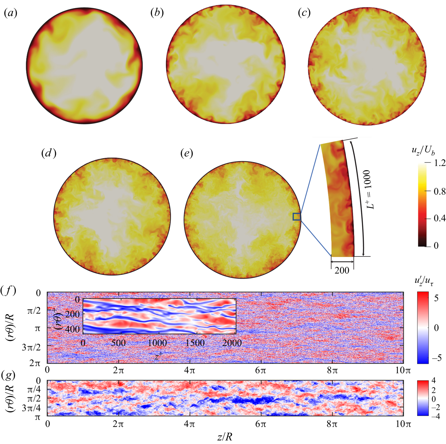
Figures 2( f,g) show the inner-scaled instantaneous axial velocity fluctuations  $u'_z/u_\tau$ on an unrolled cylindrical surface $(z-r\theta )$ for $Re_\tau \approx 5200$ at $y^+=15$ and $y/R=0.5$, respectively. At $y^+=15$, $u'_z/u_\tau$ shows the organization of the streaks, whose characteristics are better illustrated in a zoomed-in view with domain size $(2000,400)$ in wall units. Consistent with previous findings (Hellström, Sinha & Smits Reference Hellström, Sinha and Smits2011; Bernardini et al. Reference Bernardini, Pirozzoli and Orlandi2014), the flow in the outer region exhibits very long positive/negative $u'_z/u_\tau$ patches – indicating the presence of LSMs and VLSMs.
3.2. Friction factor
The mean friction (or wall shear stress), which is proportional to the pressure drop or the amount of energy required to sustain the flow, is an important parameter and has been studied extensively (Blasius Reference Blasius1913; McKeon et al. Reference McKeon, Zagarola and Smits2005; Furuichi et al. Reference Furuichi, Terao, Wada and Tsuji2015; Pirozzoli et al. Reference Pirozzoli, Romero, Fatica, Verzicco and Orlandi2021). A semi-empirical relation between the friction factor  $\lambda =8\tau _{z,w}/(\rho U^2_b)$ and $Re$ is given as (known as the Prandtl friction law)
 \begin{equation} 1/\lambda^{1/2}=A\log_{10}(Re_b\,\lambda^{1/2})-B, \end{equation}
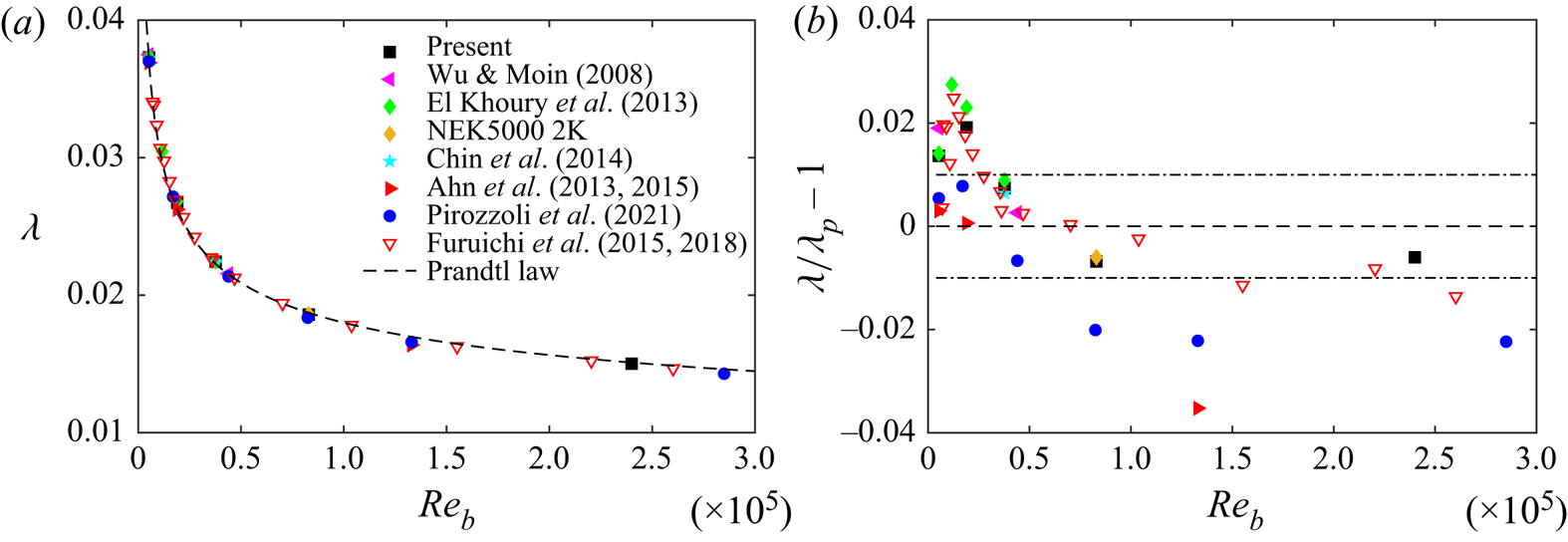
where the constant  $A$ is related to the von Kármán constant as $A=1/(2\kappa \sqrt {2} \log _{10}(e))$. Curve-fitting the experimental data over $3.1\times 10^3< Re_b<3.2\times 10^6$ by Nikuradse (Reference Nikuradse1933) yields $A=2.0$ and $B=0.8$, which corresponds to $\kappa =0.407$. However, notable deviations were observed when comparing the Prandtl friction law with other experimental data. For example, McKeon et al. (Reference McKeon, Zagarola and Smits2005) showed that for the Princeton Superpipe data (in the range $3.1\times 10^4 \leq Re_b \leq 3.5 \times 10^7$), the constants of the Prandtl law work only over a limited range of $Re_b$. New constants (i.e. $A=1.920$ and $B=0.475$) and additional $Re$-dependent corrections are needed to better fit the data in the entire $Re_b$ range. For the ‘Hi-Reff’ data, Furuichi et al. (Reference Furuichi, Terao, Wada and Tsuji2015) found that $\lambda$ deviates from the Prandtl law by approximately $2.5\,\%$ in the lower $Re_b$ region, and $-3\,\%$ in the high $Re_b$ region. In addition, $\lambda$, although agreeing with the Superpipe data in the low $Re_b$ range, deviates for $Re_b>2 \times 10^5$.
Figure 3(a) shows the friction factor  $\lambda$ as a function of $Re_b$, along with other DNS and experimental data as well as the theoretical prediction $\lambda _p$ based on (3.1). Note that these DNS results are conducted with various domain sizes, and prior studies demonstrated that its effect on one-point statistics appears limited when $L_z/R\geq 7$ (Feldmann et al. Reference Feldmann, Bauer and Wagner2018; Pirozzoli et al. Reference Pirozzoli, Romero, Fatica, Verzicco and Orlandi2021). All DNS and experimental data seem to follow $\lambda _p$. However, the scatter is better highlighted by examining the relative error with respect to the Prandtl law (i.e. $\lambda /\lambda _p-1$). As depicted in figure 3(b), all DNS data overshoot $\lambda _p$ at the low $Re_b$ (i.e. $\le 4\times 10^4$). Our data, which agree with Wu & Moin (Reference Wu and Moin2008), El Khoury et al. (Reference El Khoury, Schlatter, Noorani, Fischer, Brethouwer and Johansson2013) and Chin et al. (Reference Chin, Monty and Ooi2014) and the new simulation at $Re=2000$ using NEK5000, exceed $\lambda _p$ by approximately 2 %, while the results of Ahn et al. (Reference Ahn, Lee, Jang and Sung2013) and Pirozzoli et al. (Reference Pirozzoli, Romero, Fatica, Verzicco and Orlandi2021) are closer to $\lambda _p$ (within 1 % for $Re_b<5\times 10^4$). Pirozzoli et al. (Reference Pirozzoli, Romero, Fatica, Verzicco and Orlandi2021) attributed this discrepancy to the different grid resolutions employed in the $\theta$-direction, which is $(R\theta )^+=4\unicode{x2013}5$ in theirs and Ahn et al. (Reference Ahn, Lee, Jang and Sung2013), but $7\unicode{x2013}8$ for Wu & Moin (Reference Wu and Moin2008) and Chin et al. (Reference Chin, Monty and Ooi2014). However, the data from El Khoury et al. (Reference El Khoury, Schlatter, Noorani, Fischer, Brethouwer and Johansson2013) and our DNS have azimuthal resolutions comparable to those in Ahn et al. (Reference Ahn, Lee, Jang and Sung2013) and Pirozzoli et al. (Reference Pirozzoli, Romero, Fatica, Verzicco and Orlandi2021), but produce results similar to Wu & Moin (Reference Wu and Moin2008) and Chin et al. (Reference Chin, Monty and Ooi2014) – suggesting that the azimuthal resolution is not the main reason for such discrepancy. Interestingly, the data of Ahn et al. (Reference Ahn, Lee, Jang and Sung2013) and Pirozzoli et al. (Reference Pirozzoli, Romero, Fatica, Verzicco and Orlandi2021) are consistently lower than our and other results in the whole $Re_b$ range. In particular, at the highest $Re_b$, the Pirozzoli et al. (Reference Pirozzoli, Romero, Fatica, Verzicco and Orlandi2021) data undershoot by 2 % from $\lambda _p$, but our data are lower by only approximately 0.6 %. Table 3 asserts that such differences in $\lambda$ are beyond the uncertainty limit.
(a) Friction factor  $\lambda$ as a function of $Re_b$, and (b) the relative deviations from the Prandtl friction law.
Summary of values and standard deviations of some key parameters: the friction factor  $\lambda =8\tau _{z,w}/(\rho U^2_b)$; the peak of axial velocity variance $\langle{u'^2_z}\rangle^{+}_p$; the peak of the Reynolds shear stress $-\langle{u'_ru'_z}\rangle^{+}_p$; the axial $\langle{\tau '^2_{z,w}}\rangle^+$ and azimuthal $\langle{\tau '^2_{\theta,w} }\rangle^+$ wall shear stress fluctuations; and the wall ( $p'^+_{w,rms}$) and peak ( $p'^+_{p,rms}$) values of root-mean-square (r.m.s.) pressure fluctuations.

Our DNS and the experimental data of Furuichi et al. (Reference Furuichi, Terao, Wada and Tsuji2015) agree well for the  $Re_b$ range studied. Fitting our DNS data with (3.1) yields $A=2.039\pm 0.083$, $B=0.948\pm 0.364$ with uncertainty estimates based on 95 % confidence bounds, giving $\kappa =0.399\pm 0.015$. The value reported by Pirozzoli et al. (Reference Pirozzoli, Romero, Fatica, Verzicco and Orlandi2021) (i.e. $A=2.102$, $B=1.148$) are slightly larger than ours but still within the uncertainty range. However, large uncertainty is present in the fitted values due to the limited data points in $Re$. In addition, as $Re_b$ is still relatively low, the reported value of $\kappa =0.399\pm 0.015$ should not be used outside of the given $Re$ range. As will be shown in § 3.4, even for the highest $Re_b$ case, a distinct logarithmic region does not manifest itself in the mean velocity profile $U(y)$. Higher $Re$ data (e.g. $Re_\tau \ge 10^4$) are required to better estimate the constants in (3.1) and the associated $\kappa$ values.
3.3. Wall shear stress fluctuations
The  $Re$-dependence of axial wall shear stress fluctuation $\langle{\tau '^2_{z,w}}\rangle^+$ is one of the highly debated issues in wall turbulence. Note that $\langle{\tau '^2_{z,w}}\rangle^+$ is also equivalent to the wall dissipation of the axial Reynolds stress component $\epsilon ^+_{z,w}$, the azimuthal vorticity variance at the wall $\langle{\omega '^2_\theta }\rangle^+$ or the limiting value of $\langle{ u'^2_z}\rangle ^+/U^2$ at the wall (Örlü & Schlatter Reference Örlü and Schlatter2011). Previous DNS studies of channel, pipe and turbulent boundary layer observed an increase in $\langle{\tau '^2_{z,w}}\rangle^+$ with $Re_\tau$, which reflects the increased contribution of large-scale motions to wall shear stress at high $Re$ values (Marusic, Mathis & Hutchins Reference Marusic, Mathis and Hutchins2010a). However, the exact dependence of $\langle{\tau '^2_{z,w}}\rangle^+$ on $Re_\tau$ is not well established. For example, Örlü & Schlatter (Reference Örlü and Schlatter2011) suggested that the r.m.s. $\langle{\tau '^2_{z,w}}\rangle^+$ follows
 \begin{equation} \langle \tau'^2_{z,w} \rangle^{{+}1/2}=C+D\ln(Re_\tau), \end{equation}
where the two constants  $C$ and $D$ are chosen as $0.298$ and $0.018$ based on the DNS of turbulent boundary layer data.
Some works (Yang & Lozano-Durán Reference Yang and Lozano-Durán2017; Smits et al. Reference Smits, Hultmark, Lee, Pirozzoli and Wu2021) also suggested that
 \begin{equation} \langle \tau'^2_{z,w} \rangle^+=E+F\ln(Re_\tau). \end{equation}
By fitting turbulent channel flow data of Lee & Moser (Reference Lee and Moser2015) and pipe flow data of Pirozzoli et al. (Reference Pirozzoli, Romero, Fatica, Verzicco and Orlandi2021) for  $Re_\tau \ge 1000$, Smits et al. (Reference Smits, Hultmark, Lee, Pirozzoli and Wu2021) obtained $E=0.08$ and $F=0.0139$.
Recently, Chen & Sreenivasan (Reference Chen and Sreenivasan2021) proposed a defect-power law, given as
 \begin{align} \langle \tau'^2_{z,w} \rangle^+=\epsilon^+_{z,w}=G-H\,Re^{{-}1/4}_\tau, \end{align}
where  $G$ is the asymptotic value at infinite $Re$, and $H$ is a coefficient. The assumption for (3.4) is that the dissipation of the axial Reynolds stress component ( $\epsilon ^+_z=\nu \langle{(\partial u^+_z/\partial x^+_j)(\partial u^+_z/\partial x^+_j)}\rangle$) balances the turbulent kinetic energy production ( $P_k=-\langle{u_ru_z}\rangle^+(\partial U^+/\partial y^+)$) near the location of peak production. The fact that $P_k$ is bounded by $1/4$ (Sreenivasan Reference Sreenivasan1989; Pope Reference Pope2000) implies that $\epsilon ^+_{z,w}$ may also stay bounded, which is further assumed by Chen & Sreenivasan (Reference Chen and Sreenivasan2021) to be the same bound of $P_k$, i.e. $G=1/4$ (Chen & Sreenivasan Reference Chen and Sreenivasan2021). This argument was later criticized by Smits et al. (Reference Smits, Hultmark, Lee, Pirozzoli and Wu2021) for the following two reasons. First, based on the DNS data, the location of peak production is actually the place where the largest imbalance of production and dissipation occurs. Second, as the balance between different terms in the Reynolds stress transport equation changes rapidly near the wall, it is unclear how the balance between $P_k$ and $\epsilon ^+_{z,w}$ can be extended up to the wall, where $P_k=0$, and $\epsilon ^+_{z,w}$ equals the viscous diffusion.
The axial wall shear stress fluctuation  $\langle{\tau '^2_{z,w}}\rangle^+$ as a function of $Re_\tau$ is depicted in figure 4(a). Akin to the observation in El Khoury et al. (Reference El Khoury, Schlatter, Noorani, Fischer, Brethouwer and Johansson2013), the values for the pipe are slightly lower than those for the channel, but the difference decreases with increasing $Re_\tau$. Note that the data of Pirozzoli et al. (Reference Pirozzoli, Romero, Fatica, Verzicco and Orlandi2021) are slightly lower than others, which is consistent with the lower $\lambda$ in figure 3. The logarithmic law (3.2) proposed by Örlü & Schlatter (Reference Örlü and Schlatter2011) is higher than the DNS data. This is somehow expected as the fitting coefficients were obtained based on the DNS of turbulent boundary layer data, which are higher than in pipe and channel. In the high $Re_\tau$ range, both the logarithmic (3.3) and defect-power-law scalings (3.4) agree well with the data. However, both scalings exhibit notable disagreements in the low $Re_\tau$ range. The discrepancy seems not particularly surprising, given that the parameters in these equations are obtained from different datasets and different $Re_\tau$ ranges. As a reference, the inset in figure 4(a) shows the fitting results of (3.2)–(3.4) using our DNS data only. The fitted values are $C=0.225$, $D=0.0264$ for (3.2), $E=0.016$, $F=0.0218$ for (3.3), and $G=0.255$, $H=0.477$ for (3.4). For the $Re_\tau$ range studied, the data seem to match better the defect-power law but with a slightly higher asymptotic value than suggested by Chen & Sreenivasan (Reference Chen and Sreenivasan2021). Additional data at higher $Re_\tau$ are needed to confirm this finding.
(a) Axial ( $\langle \tau '^2_{z,w}\rangle ^+$) and (b) azimuthal ( $\langle \tau '^2_{\theta,w}\rangle ^+$) wall shear stress fluctuations as a function of $Re_\tau$. The dotted, dashed and dashed-dotted lines in the inset of (a) denote $\langle \tau '^2_{z,w}\rangle ^+=(0.225+0.0264 \ln (Re_\tau ))^2$, $\langle \tau '^2_{z,w}\rangle ^+=0.016+0.0218 \ln (Re_\tau )$ and $\langle \tau '^2_{z,w}\rangle ^+=0.255-0.477\,Re^{-1/4}_\tau$, respectively.
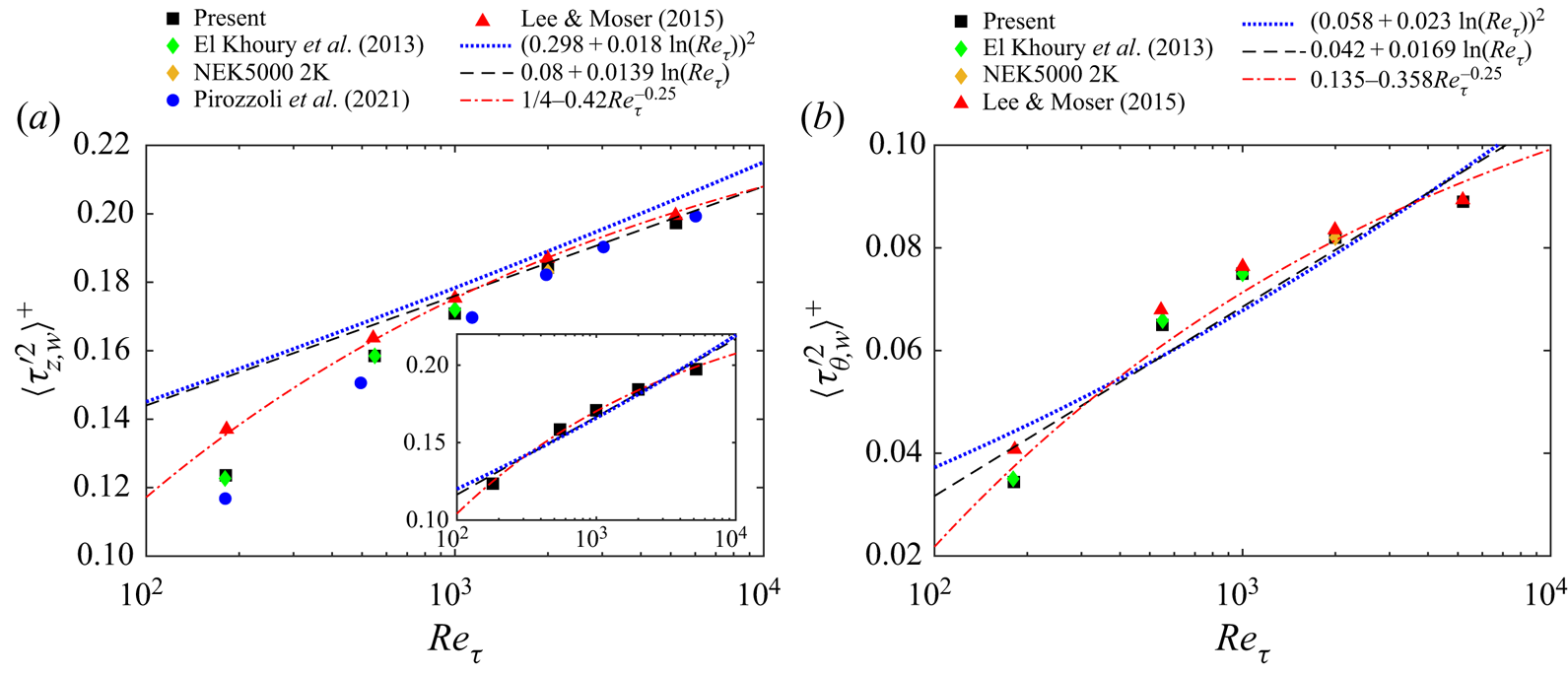
Figure 4(b) further shows the azimuthal wall shear stress fluctuation  $\langle \tau '^2_{\theta,w} \rangle ^+$ as a function of $Re_\tau$. Similar to findings for $\langle{\tau '^2_{z,w}}\rangle^+$, our data agree well with El Khoury et al. (Reference El Khoury, Schlatter, Noorani, Fischer, Brethouwer and Johansson2013) and NEK5000 2K cases, and all of them become closer to Lee & Moser (Reference Lee and Moser2015) with increasing $Re_\tau$. Fitting data with the logarithmic and defect-power law yields $\langle \tau '^2_{\theta,w} \rangle ^+=(0.058+0.023\ln (Re_\tau ))^2$, $\langle \tau '^2_{\theta,w} \rangle ^+=-0.040+0.016\ln (Re_\tau )$ and $\langle \tau '^2_{\theta,w} \rangle ^+=0.135-0.353\,Re^{-1/4}_\tau$. Again, the defect-power law seems to match better the DNS data, but the agreement is not as good as for $\langle{\tau '^2_{z,w}}\rangle^+$.
3.4. Mean velocity profile
In an overlap region between the inner and outer flows, there is a logarithmic variation of the mean axial velocity  $U^+$ profile, which is given as
 \begin{equation} U^+=\frac{1}{\kappa} \ln y^+{+}B. \end{equation}
In a true log layer, the indicator function  $\beta =y^+( \partial U^+/\partial y^+)$ is constant and equals $1/\kappa$.
The  $U^+$ profiles at different $Re_\tau$ are compared to previous DNS data in figure 5(a). First, as expected, the wake in $U^+$ for the pipe is stronger than in the channel by Lee & Moser (Reference Lee and Moser2015). Second, our data in the outer region agree well with those of El Khoury et al. (Reference El Khoury, Schlatter, Noorani, Fischer, Brethouwer and Johansson2013), but not with Pirozzoli et al. (Reference Pirozzoli, Romero, Fatica, Verzicco and Orlandi2021). This discrepancy was also noted by Pirozzoli et al. (Reference Pirozzoli, Romero, Fatica, Verzicco and Orlandi2021), who found that their data, along with those of Wu & Moin (Reference Wu and Moin2008) and Ahn et al. (Reference Ahn, Lee, Jang and Sung2013), differ from those of El Khoury et al. (Reference El Khoury, Schlatter, Noorani, Fischer, Brethouwer and Johansson2013) and Chin et al. (Reference Chin, Monty and Ooi2014). This disparity is probably due to the numerical methods, where all of the former used low-order finite difference methods, while the latter two used high-order spectral-element methods.
(a) Mean velocity profiles  $U^+$ and (b) log-law diagnostic function $\beta$. Profiles in (a) are offset vertically by two wall units, and the shaded area in (b) represents the standard deviation of our data at $Re_\tau =5200$.
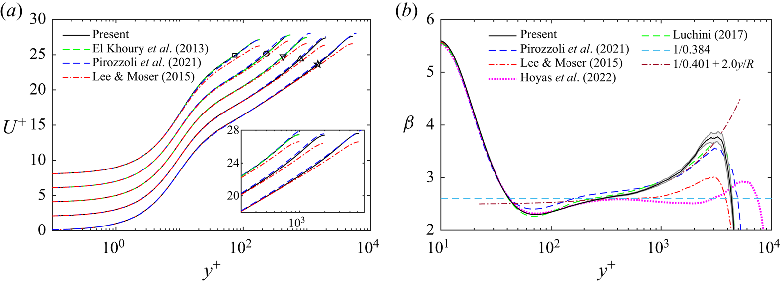
The log-law diagnostics function  $\beta$ is shown in figure 5(b) for all high DNS data (i.e. $Re_\tau >5000$). Interestingly, $\beta$ for our $Re_\tau \approx 5200$ agrees with the channel data of Lee & Moser (Reference Lee and Moser2015) and Hoyas et al. (Reference Hoyas, Oberlack, Alcántara-Ávila, Kraheberger and Laux2022) up to $y^+\approx 250$. Note that a relatively small domain size was used by Hoyas et al. (Reference Hoyas, Oberlack, Alcántara-Ávila, Kraheberger and Laux2022), but it is assumed large enough to yield accurate flow statistics (Lozano-Durán & Jiménez Reference Lozano-Durán and Jiménez2014). This suggests a near-wall universality of the inner scaled mean velocity – similar to that observed by Monty et al. (Reference Monty, Hutchins, Ng, Marusic and Chong2009). For all three cases, the trough is $\beta \approx 2.30$, located at $y^+\approx 70$. However, the data of Pirozzoli et al. (Reference Pirozzoli, Romero, Fatica, Verzicco and Orlandi2021) deviate from others for $y^+>40$ and have a larger magnitude of the trough, which is somewhat consistent with the slight upward shift of the $U^+$ observed in figure 5(a). This discrepancy is significantly larger than the statistical uncertainty (see Appendix B). Unlike channel flow, where a plateau starts to develop for $Re_\tau \ge 5200$, there is no plateau for pipe flow – suggesting that the minimum $Re_\tau$ for $U^+$ to develop a logarithmic region should be higher in the pipe than in the channel. The $\beta$ in the wake region of the pipe is distinctly larger than the channel, implying a notable difference in flow structures in the core region between these two flows (Chin et al. Reference Chin, Monty and Ooi2014).
High-order corrections to the log-law relation (3.5) were sometimes introduced to better describe the mean velocity profile in the overlap region (Buschmann & Gad-el Hak Reference Buschmann and Gad-el Hak2003; Luchini Reference Luchini2017; Cantwell Reference Cantwell2019). For example, based on refined overlap arguments expressed by Afzal & Yajnik (Reference Afzal and Yajnik1973), Jiménez & Moser (Reference Jiménez and Moser2007) proposed the indicator function
 \begin{align} \beta=\left(\frac{1}{\kappa_\infty}+\frac{\alpha_1}{Re_\tau}\right)+\alpha_2\,\frac{y}{R}, \end{align}
where  $\alpha _1$ and $\alpha _2$ are adjustable constants, and $\kappa _\infty$ is the asymptotic von Kármán constant. Equation (3.6) allows for a $Re$-dependence of $\kappa =\kappa _\infty +(\alpha _1/Re_\tau )^{-1}$ and introduces a linear dependence on $y$. By fitting our $Re_\tau \approx 5200$ data in the region between $y^+=300$ and $y=0.16$, we obtain $\kappa =0.401$ and $\alpha _2=2.0$. This $\kappa$ is very close to $0.399$ estimated from the friction factor relation (3.1) and $0.402$ reported by Jiménez & Moser (Reference Jiménez and Moser2007) using channel data of $Re_\tau =1000$ from Del Alamo et al. (Reference Del Alamo, Jiménez, Zandonade and Moser2004), and $Re_\tau =2000$ from Hoyas & Jiménez (Reference Hoyas and Jiménez2006). It is slightly larger than $0.387$ by Pirozzoli et al. (Reference Pirozzoli, Romero, Fatica, Verzicco and Orlandi2021) and $0.384$ by Lee & Moser (Reference Lee and Moser2015). In addition, $\alpha _2$ is generally much larger in the pipe than in the channel – suggesting a strong geometry effect on $\beta$. The value of $\alpha _2=2$ is consistent with the finding by Luchini (Reference Luchini2017), who suggested that the logarithmic law of the velocity profile is universal across different geometries of wall turbulence, provided that the perturbative effect of the pressure gradient is taken into consideration. Furthermore, a good collapse between our data and the analytical prediction by Luchini (Reference Luchini2017) is seen in figure 5(b).
3.5. Reynolds stresses
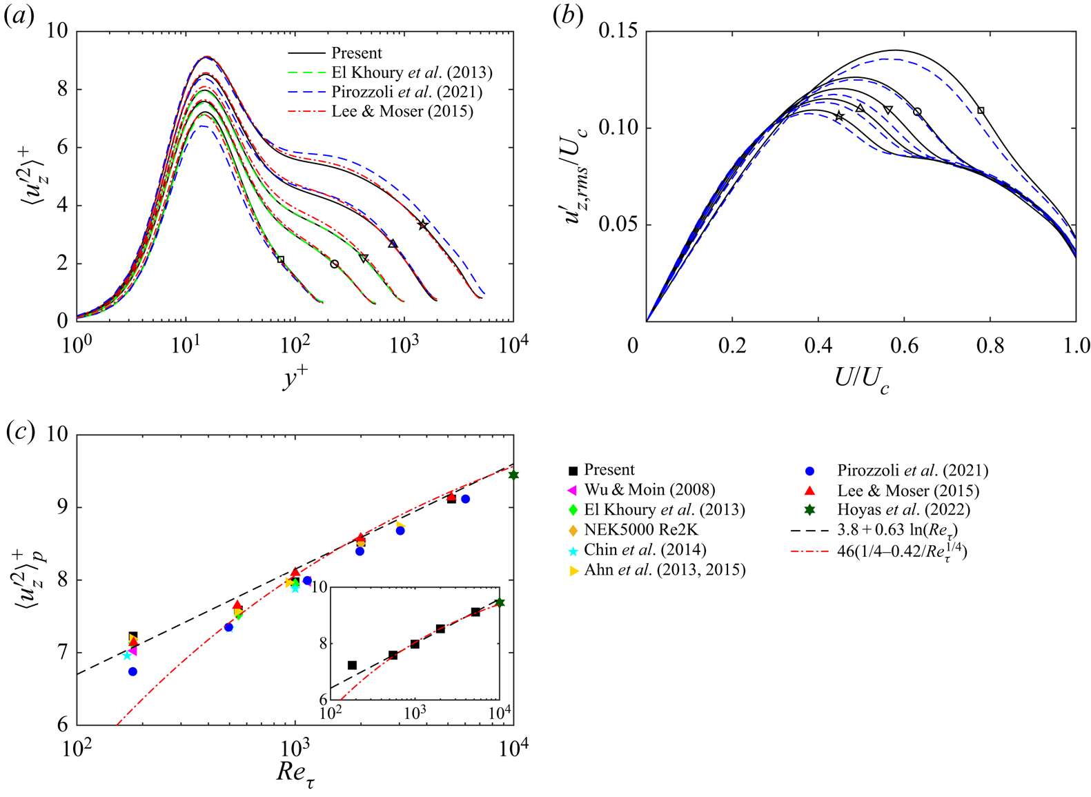
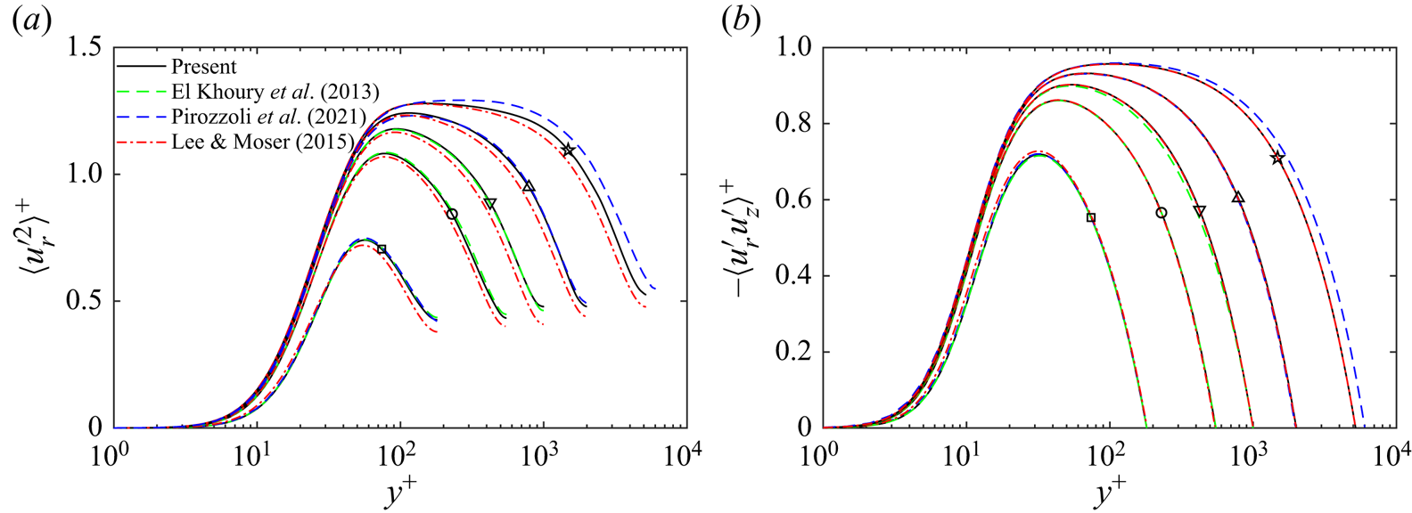
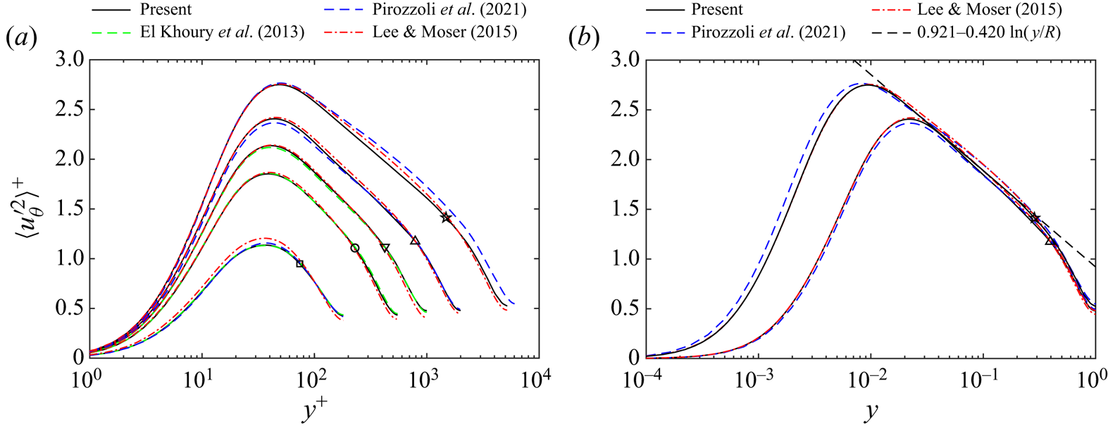
The non-zero components of the Reynolds stress tensor (or the velocity variances and covariance) are examined in this subsection (figures 6–10). For all datasets, the inner-scaled velocity variances and covariance increase with  $Re_\tau$ in the whole wall-normal range. In terms of the axial velocity variance $\langle{u'^2_z}\rangle^{+}$ (figure 6a), our data agree well with El Khoury et al. (Reference El Khoury, Schlatter, Noorani, Fischer, Brethouwer and Johansson2013) but differ from Pirozzoli et al. (Reference Pirozzoli, Romero, Fatica, Verzicco and Orlandi2021), which is notably smaller in the near-wall region, particularly at low $Re_\tau$. For the highest $Re_\tau$ cases, the agreement is reasonably good near the wall. However, note that the Pirozzoli et al. (Reference Pirozzoli, Romero, Fatica, Verzicco and Orlandi2021) simulation is at a slightly higher $Re_\tau$ (i.e. $\sim 6000$). The differences between our case and that of Pirozzoli et al. (Reference Pirozzoli, Romero, Fatica, Verzicco and Orlandi2021) can be better highlighted in the diagnostic plot (figure 6b), where the r.m.s. axial velocity fluctuation $u'_{z,rms}$ is plotted against the mean velocity $U^+$. The diagnostic plot was introduced by Alfredsson & Örlü (Reference Alfredsson and Örlü2010) to assess if the mean velocity and velocity fluctuation profiles behave correctly without the need to determine the friction velocity or the wall position. Consistent with the observation in Alfredsson & Örlü (Reference Alfredsson and Örlü2010), the diagnostic plot collapses in the outer region for $Re_\tau >180$, and has a clear $Re$ trend around the peak value. Most importantly, the data by Pirozzoli et al. (Reference Pirozzoli, Romero, Fatica, Verzicco and Orlandi2021) are consistently lower than ours, particularly in the near-wall region. Such inconsistency is also observed for $\langle{u'^2_\theta}\rangle^{+}$ (figure 10). The agreement for $\langle{u'^2_r}\rangle^{+}$ (figure 7a) is reasonably good among different pipe flow datasets, which is slightly larger than the channel, particularly in the outer region. The Reynolds shear stress $\langle{u'_r u'_z}\rangle^+$ shows excellent agreement among different datasets, even including the channel.
(a) Axial velocity variance  $\langle{ u'^2_z}\rangle ^+$ as a function of $y^+$; (b) the diagnostic plot depicting $u'_{z,rms}/U_c$ as a function of $U^+/U_c$; and (c) the inner peak of axial velocity variance $\langle{ u'^2_z}\rangle ^+_p$ as a function of $y^+$. The dashed and dashed-dotted lines in the inset of (c) denote $\langle{u'^2_z}\rangle^{+}_p=3.251+0.687\ln (Re_\tau )$ and $\langle{u'^2_z}\rangle^{+}_p=11.132-17.402\,Re^{-1/4}_\tau$, respectively.
(a) Radial velocity variance  $\langle u'^2_r \rangle ^+$, and (b) Reynolds shear stress $\langle u'_r u'_z \rangle ^+$, as functions of $y^+$.
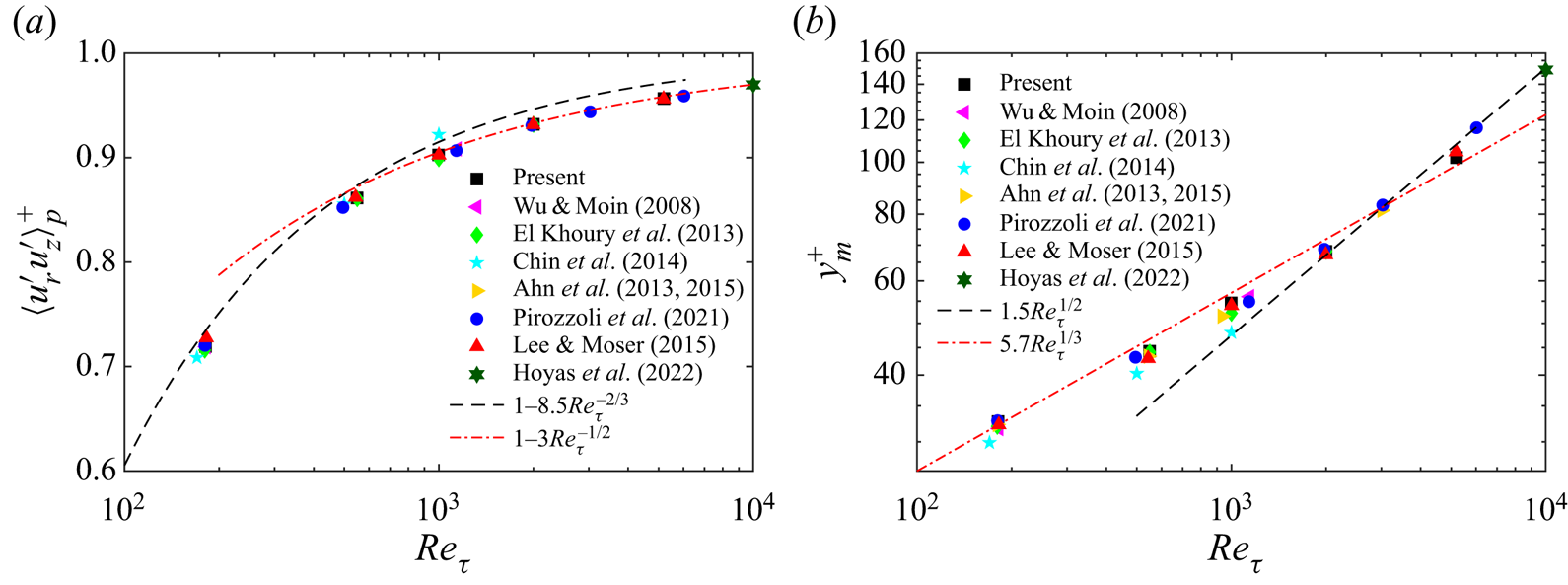
Reynolds number dependence of (a) the peak of the Reynolds shear stress  $\langle u'_r u'_z \rangle ^+$, and (b) the corresponding peak location in wall units.
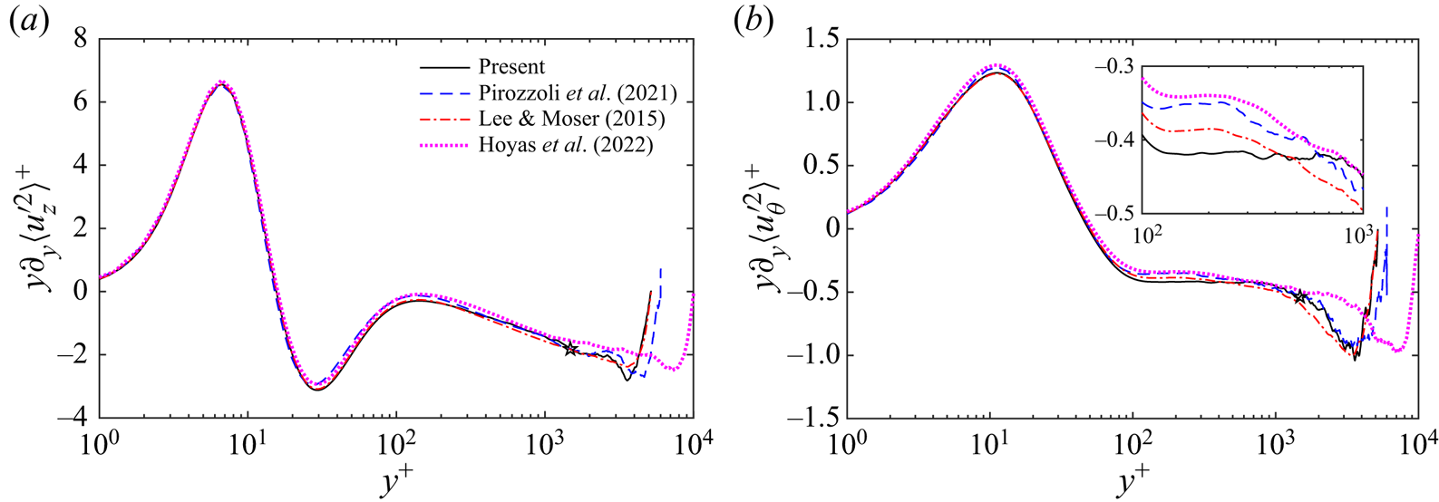
Indicator function for Townsend's prediction among different high- $Re$ simulations: (a) axial velocity variance $y\,\partial _y\langle{ u'^2_z}\rangle ^+$, and (b) azimuthal velocity variance $y\,\partial _y\langle u'^2_\theta \rangle ^+$.
Azimuthal velocity variance  $\langle u'^2_\theta \rangle ^+$ as a function of (a) $y^+$ and (b) $y/R$. Only the two highest $Re_\tau$ cases are included in (b).
Let us focus now on the inner peak of the axial velocity variance  $\langle{u'^2_z}\rangle^{+}$. The inner peak is assumed to increase logarithmically with $Re_\tau$ – similar to the wall shear stress fluctuations due to the increased modulation effect of the large-scale structures in the logarithmic layer (Marusic & Monty Reference Marusic and Monty2019). Chen & Sreenivasan (Reference Chen and Sreenivasan2021) suggested recently that the growth of $\langle{u'^2_z}\rangle^{+}$ would eventually saturate. The argument is based on the balance between the viscous diffusion and dissipation at the wall, and the Taylor series expansion of the axial velocity variance near the wall, given as
 \begin{equation} \langle{u'^2_z}\rangle^+\sim D^+_{z,w}y^{{+}2}= \epsilon^+_{z,w} y^{{+}2}. \end{equation}
Note that a similar expression is obtained in Smits et al. (Reference Smits, Hultmark, Lee, Pirozzoli and Wu2021), where the axial wall dissipation is used instead, i.e.  $\langle{u'^2_z}\rangle^{+}\sim \langle{\tau '^2_{z,w}}\rangle^+y^{+2}$. If the assumption of the boundedness of wall dissipation (3.4) is valid and the inner peak location of $\langle{u'^2_z}\rangle^{+}$ (denoted as $y^+_{z,p}$) is independent of $Re_\tau$, then (3.7) suggests that the peak of axial velocity variance should also be bounded in a defect-power form similar to the wall shear stress fluctuation:
 \begin{align} \langle{u'^2_z}\rangle^+_p=M- N\,Re_\tau^{{-}1/4}, \end{align}
where  $M$ is the asymptotic value and $N$ is the coefficient.
This validity of (3.8) was challenged recently by Pirozzoli et al. (Reference Pirozzoli, Romero, Fatica, Verzicco and Orlandi2021), who, based on their data, observed a slight increase of  $y^+_{z,p}$ with $Re_\tau$, from $y^+_{z,p}=14.28$ for $Re_\tau \approx 500$ to $15.14$ for $Re_\tau \approx 6000$. We emphasize that such variation of $y^+_{z,p}$ with $Re_\tau$ is not observed in our case, where much finer near-wall resolutions than in Pirozzoli et al. (Reference Pirozzoli, Romero, Fatica, Verzicco and Orlandi2021) are used. The value of $y^+_{z,p}$ is approximately $15$ for all $Re_\tau$ (e.g. $y^+_{z,p}=15.07$, $15.03$, $15.50$ for $Re_\tau =180$, $2000$, $5000$, respectively) – akin to the findings by many others (Moser et al. Reference Moser, Kim and Mansour1999; Jiménez et al. Reference Jiménez, Hoyas, Simens and Mizuno2010; Chin et al. Reference Chin, Monty and Ooi2014; Smits et al. Reference Smits, Hultmark, Lee, Pirozzoli and Wu2021).
Figure 6(c) shows  $\langle{u'^2_z}\rangle^{+}_p$ for all the DNS data listed in table 2, along with the logarithmic law $\langle{u'^2_z}\rangle^{+}_p=3.8+0.64\ln (Re_\tau )$ by Marusic et al. (Reference Marusic, Baars and Hutchins2017) and the power law $\langle{u'^2_z}\rangle^{+}_p=11.5-19.32Re_\tau ^{-1/4}$ by Chen & Sreenivasan (Reference Chen and Sreenivasan2021). The difference between different DNS datasets is relatively small, except for those from Pirozzoli et al. (Reference Pirozzoli, Romero, Fatica, Verzicco and Orlandi2021), which are consistently lower than others for all $Re_\tau$. Note that this discrepancy is much larger than the uncertainty (standard deviation), which is less than $0.5\,\%$ (see table 3). Both the logarithmic and defect-power laws fit well with the data in the high $Re_\tau$ range but have certain discrepancies at low $Re_\tau$. This suggests that there might exist a transitional scaling – similar to that found for the Reynolds shear stress (Chen, Hussain & She Reference Chen, Hussain and She2019). The parameters in these two scaling laws can be adjusted to better fit our dataset. The inset shows the fitting results for our data without the one at $Re_\tau =180$: $\langle{u'^2_z}\rangle^{+}_p=3.251+0.687\ln (Re_\tau )$ and $\langle{u'^2_z}\rangle^{+}_p=11.132-17.402\,Re^{-1/4}_\tau$. With these new constants, the agreement is improved for both scaling laws. In summary, for the $Re_\tau$ range studied, both scaling laws provide a good match with $\langle{u'^2_z}\rangle^{+}_p$ data when the fitting parameters are properly adjusted. Data at even higher $Re_\tau$ are required to determine which law is more consistent with the data.
According to Townsend's attached eddy hypothesis, at sufficiently high  $Re$, the Reynolds stress components in a certain $y$ range satisfy
 $$\begin{gather} \langle{u'^2_z}\rangle^+=A_1-B_1 \ln(y/R), \end{gather}$$
 $$\begin{gather}\langle{u'^2_z}\rangle^+=A_2, \end{gather}$$
 $$\begin{gather}\langle{u'^2_\theta}\rangle^+=A_3-B_3 \ln(y/R), \end{gather}$$
 $$\begin{gather}\langle{u'_r u'_z}\rangle^+=-1, \end{gather}$$
where  $A_i$ and $B_i$ are universal constants.
Consistent with these relations, the radial velocity variance  $\langle{u'^2_r}\rangle^{+}$ slowly develops a flat region as $Re_\tau$ increases. In addition, the Reynolds shear stress $\langle{-u'_ru'_z}\rangle^+$ profiles also tend to become flattened at higher $Re_\tau$. As noted by Afzal (Reference Afzal1982), the peak Reynolds shear stress at high $Re_\tau$ follows $\langle{-u'_ru'_z}\rangle^+_p\approx 1-2/\sqrt {\kappa \,Re_\tau }$, and the corresponding position $y^+_m$ shifts away from the wall following $y^+_m\sim \sqrt {Re_\tau /\kappa }$. Chen et al. (Reference Chen, Hussain and She2019) suggested that there is a non-universal scaling transition, where the peaks at low $Re_\tau$ scales as $\langle{u'_ru'_z}\rangle^{+}_p\approx Re_\tau ^{-2/3}$ and their locations scales as $y^+_m \sim Re_\tau ^{1/3}$. Figure 8 shows $\langle{-u'_ru'_z}\rangle^+_p$ and the corresponding $y^+_m$ as a function of $Re_\tau$. For $Re_\tau >1000$, $Re^{-1/2}$ for $\langle{-u'_ru'_z}\rangle^+_p$ and $Re^{-1/2}$ for $y^+_m$ are satisfied with good accuracy, and at the low $Re_\tau$ range, $Re^{-2/3}_\tau$ for $\langle{-u'_ru'_z}\rangle^+_p$ and $Re^{-1/3}_\tau$ for $y^+_m$ scalings proposed by Chen et al. (Reference Chen, Hussain and She2019) also yield good agreement.
Regarding the axial velocity variance  $\langle{ u'^2_z}\rangle ^+$, the indicator function is not flat anywhere in the domain (figure 9a) – suggesting that no clear logarithmic region develops for the $Re_\tau$ range considered. As discussed in Lee & Moser (Reference Lee and Moser2015), $Re_\tau =5200$ is not quite high enough to exhibit such a region. Based on the Superpipe data, Marusic et al. (Reference Marusic, Monty, Hultmark and Smits2013) suggested that a sensible logarithmic layer emerges only for $Re_\tau >10^4$. Consistent with the findings in Lee & Moser (Reference Lee and Moser2015) and Pirozzoli et al. (Reference Pirozzoli, Romero, Fatica, Verzicco and Orlandi2021), the azimuthal velocity variance $\langle u'^2_\theta \rangle ^+$ develops the logarithmic layer at lower $Re_\tau$. The indicator function of $\langle u'^2_\theta \rangle ^+$ shows a distinct plateau (figure 9b). Interestingly, when compared with other cases, the range of the logarithmic layer is wider in our $Re_\tau \approx 5200$ case. Fitting the data in the range $120\le y^+ \le 800$ yields $A_3=0.921$, $B_3=0.420$, which are close to $A_3=1.0$, $B_3=0.40$ by Pirozzoli et al. (Reference Pirozzoli, Romero, Fatica, Verzicco and Orlandi2021), and between $A_3=1.08$, $B_3=0.387$ obtained by Lee & Moser (Reference Lee and Moser2015) for the turbulent channel and $A_3=0.8$, $B_3=-0.45$ by Sillero, Jiménez & Moser (Reference Sillero, Jiménez and Moser2013) in the turbulent boundary layer.
3.6. Production and dissipation of the turbulent kinetic energy
Figure 11(a) shows the production  $P^+_k$ and dissipation $\epsilon ^+_k\ (=\nu \langle{(\partial u'^+_i/\partial x^+_j)(\partial u'^+_i/\partial x^+_j)}\rangle)$ of the turbulent kinetic energy (i.e. $k^+=(\langle u'^2_r \rangle ^++\langle u'^2_\theta \rangle ^++\langle{ u'^2_z}\rangle ^+)/2$). Other terms in the transport equations of the turbulent kinetic energy and individual Reynolds stress components are available at https://dataverse.tdl.org/dataverse/turbpipe. The production $P^+_k$ has a peak at around $y^+\approx 11$, and the magnitude approaches the asymptotic value $1/4$ as $Re_\tau$ increases. Despite notable differences in the mean axial/streamwise velocity profile observed in the outer region, $P^+_k$ is quite similar between pipes and channels. This explains why the higher velocity gradient of the pipe does not contribute an effect to the turbulence intensities. The magnitude of dissipation $\epsilon ^+_k$ increases continuously with $Re_\tau$, and the difference between the pipe and channel is mainly in the near-wall region and decreases with increasing $Re_\tau$.
(a) Production  $P^+_k$ and dissipation $\epsilon ^+_k$ of the turbulent kinetic energy, and (b) balance of production and dissipation $P^+_k/\epsilon ^+_k-1$, as functions of $y^+$.
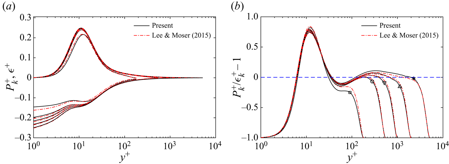
At sufficiently high  $Re_\tau$, there is an intermediate region where production balances dissipation. Recent numerical results (Lee & Moser Reference Lee and Moser2015; Pirozzoli et al. Reference Pirozzoli, Romero, Fatica, Verzicco and Orlandi2021) suggest that such equilibrium between production and dissipation is violated due to the presence of LSMs and VLSMs. Figure 11(b) shows the relative excess of production over dissipation ( $P^+_k/\epsilon ^+_k-1$). First, there is a near-wall region ( $8\le y^+\le 35$) where $P^+_k$ distinctly exceeds $\epsilon ^+_k$. At high $Re_\tau$, another region of $P^+_k/\epsilon ^+_k>1$ develops, and the magnitude increases with $Re_\tau$. For the $Re_\tau \approx 5200$ case, the peak imbalance is approximately $11\,\%$ (located at $y^+\approx 330$), which is slightly larger than in the channel (i.e. $8\,\%)$.
3.7. Mean pressure and r.m.s. pressure fluctuation
The mean pressure and r.m.s. pressure fluctuations are displayed in figure 12. First, the mean pressure  $P^+$ has different behaviour in the outer region between pipe and channel flows, with $P^+$ being substantially lower in the wake of the pipe. As discussed in El Khoury et al. (Reference El Khoury, Schlatter, Noorani, Fischer, Brethouwer and Johansson2013), this difference is related to the mean radial momentum equation, which, in pipe flow, is given as (Hinze Reference Hinze1975)
 \begin{equation} \frac{1}{\rho}\,\frac{\partial P}{\partial r}+\frac{\mathrm{d}}{\mathrm{d} r}\langle{u'^2_r }\rangle+\frac{\langle{u'^2_r }\rangle-\langle{u'^2_\theta }\rangle}{r}=0. \end{equation}
By changing variable (i.e.  $r=R-y$) and then integrating the above equation, the mean pressure for pipe flow with the wall value set to zero can be expressed as
 \begin{equation} P^+(y)={-}\langle{u'^2_r}\rangle^+{+}\int^y_0\frac{\langle{u'^2_r }\rangle^+{-}\langle{u'^2_\theta}\rangle}{R-y'}^+\, \mathrm{d} y'. \end{equation}
In channel flow, the last term on the left-hand side of (3.13) is absent, and the mean pressure is solely balanced by the wall-normal velocity fluctuation, i.e.  $P^+(y)=-\langle{v'^2}\rangle^+$. From figure 7(a), it is clear that the wall-normal velocity fluctuation is comparable between pipe and channel flows. However, as $\langle{u'^2_r}\rangle^+<\langle{u'^2_\theta}\rangle^{+}$ in pipe flow, the extra term in (3.14) is zero at the wall and decreases with increasing $y$ – resulting in a lower pressure in pipes than in channels.
(a) Mean pressure ( $P^+$) and (b) r.m.s. pressure fluctuation ( $P^{\prime+}_{rms}$), as functions of $y^+$.
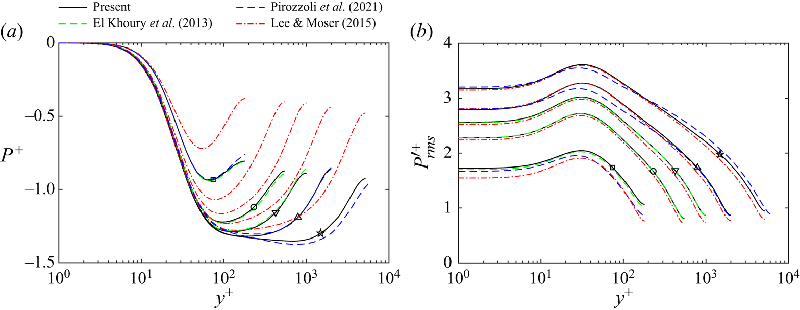
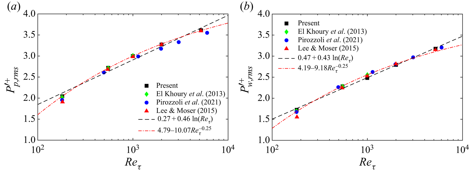
Similar to that observed by El Khoury et al. (Reference El Khoury, Schlatter, Noorani, Fischer, Brethouwer and Johansson2013), the r.m.s. pressure fluctuation  $p'^{+}_{rms}$ exhibits similar behaviour between the pipe and channel, except for slightly lower values for the latter. Minor differences are observed between our data and those of Pirozzoli et al. (Reference Pirozzoli, Romero, Fatica, Verzicco and Orlandi2021), particularly near the peak value. The difference between our data and the channel data of Lee & Moser (Reference Lee and Moser2015) in the near-wall region decreases with increasing $Re_\tau$. Figure 13 further shows the peak and wall values of $p'^+_{rms}$, which has similar $Re$-dependence as for other measures, such as wall shear stress fluctuations and axial velocity variances. Again, for the $Re_\tau$ studied, both the logarithmic and defect-power laws fit the data well.
Reynolds number dependence of (a) peak ( $P^{\prime+}_{p,rms}$) and (b) wall ( $P'^+_{w,rms}$) values of r.m.s. pressure fluctuations.
3.8. Energy spectra
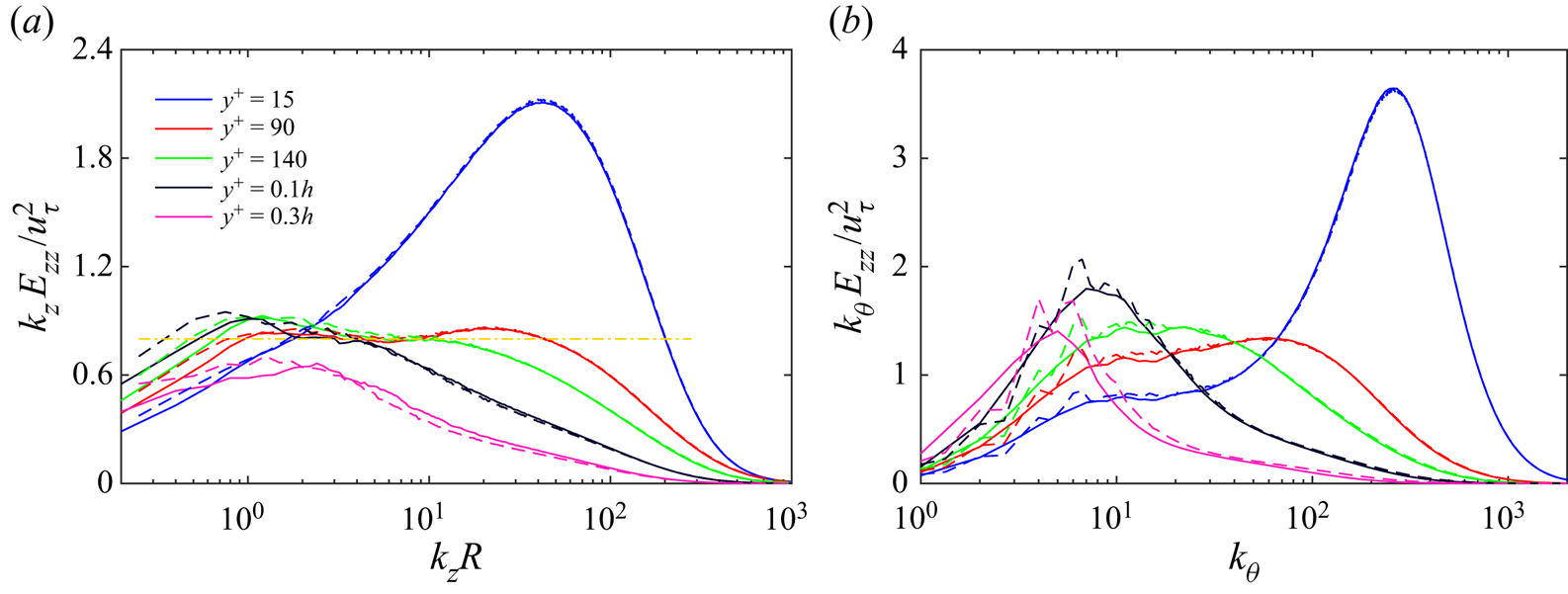
As  $Re$ increases, the separation of scales between the near-wall and outer-layer structures enlarges. In this section, the scale-separation is examined with one-dimensional velocity spectra for $Re_\tau \approx 5200$ (figure 14). The energy spectrum of axial velocity $u_z$ in the axial direction has two distinct peaks – the inner one located at $k_zR=40$ ( $\lambda ^+_z=816$) and $y^+=13$, and the outer one at $k_zR=1$ ( $\lambda _z=2{\rm \pi} R$), $y^+=400$. The dual-peak nature is more discernible in the azimuthal spectra with peaks at $k_\theta =250$ ( $\lambda ^+_\theta =2{\rm \pi} r^+/k_\theta =131$), $y^+=13$ and $k_\theta =6$ ( $\lambda _\theta =2{\rm \pi} r/k_\theta =0.846R$), $y^+=1000$. The $k_\theta$ values of all these peaks coincide with those found by Lee & Moser (Reference Lee and Moser2015) in the channel at the same $Re_\tau$, but the physical scales are smaller than in the channel. It is well known that the inner peak at $y^+=13$ is associated with the streaks that are generated through the near-wall self-sustaining cycle (Waleffe Reference Waleffe1997; Schoppa & Hussain Reference Schoppa and Hussain2002). As seen frequently in experiments (Hutchins & Marusic Reference Hutchins and Marusic2007; Monty et al. Reference Monty, Hutchins, Ng, Marusic and Chong2009; Rosenberg et al. Reference Rosenberg, Hultmark, Vallikivi, Bailey and Smits2013), the outer peak results from VLSMs. The outer peak in the $\theta$-direction (at $y=0.192$) is located farther away than the streamwise one (at $y=0.077$), which according to Wu, Baltzer & Adrian (Reference Wu, Baltzer and Adrian2012) suggests that the VLSMs in the outer region maintain their energy in the $\theta$-direction more strongly than in the $z$-direction. The pre-multiplied energy spectra of the Reynolds shear stress in axial ( $k_zE_{rz}/u^2_\tau$) and azimuthal ( $k_\theta E_{rz}/u^2_\tau$) directions as functions of $y^+$ are shown in figures 14(c,d), respectively. The inner peak is located at $y^+=30$ with $k_z R=49.2$ ( $\lambda ^+_\theta =664$) for $k_zE_{rz}/u^2_\tau$, and $k_\theta =268$ ( $\lambda ^+_\theta =120$) for $k_\theta E_{rz}/u^2_\tau$. Compared with the axial velocity spectra, although the wavelength of the outer peak remains identical, the magnitude is much weaker and farther away from the wall.
Wavenumber pre-multiplied energy spectra for  $Re_\tau =5200$: (a) $k_zE_{zz}/u^2_\tau$, (b) $k_\theta E_{zz}/u^2_\tau$, (c) $k_zE_{rz}/u^2_\tau$, and (d) $k_\theta E_{rz}/u^2_\tau$.
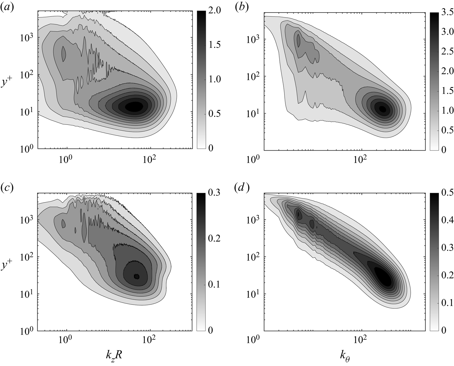
Figure 15(a) shows the one-dimensional pre-multiplied energy spectra  $k_zE_{zz}/u^2_\tau$ at different $y$ locations. For comparison, the channel data of Lee & Moser (Reference Lee and Moser2015) at the same $Re_\tau$ are also included. First, good agreement is observed at $y^+=15$ between channel and pipe, particularly at higher wavenumbers – suggesting insignificance of pipe curvature on fine-scale near-wall structures. The scaling analysis of Perry, Henbest & Chong (Reference Perry, Henbest and Chong1986) suggests that the energy spectral density of the axial velocity fluctuations $k_zE_{zz}/u^2_\tau$ should vary as $k^{-1}_z$ in the overlap region. The $k^{-1}_z$ region has previously been observed in the high- $Re$ experiments (Nickels et al. Reference Nickels, Marusic, Hafez and Chong2005; Rosenberg et al. Reference Rosenberg, Hultmark, Vallikivi, Bailey and Smits2013). Recently, such $k^{-1}_z$ has also been discovered in DNS of turbulent channel flow at $Re_\tau =5200$ (Lee & Moser Reference Lee and Moser2015). Similarly, a plateau in the region $6\le k_zR\le 10$ is observed for $90\le y^+\le 170$, and the magnitude $0.8$ agrees with experiments (Nickels et al. Reference Nickels, Marusic, Hafez and Chong2005; Rosenberg et al. Reference Rosenberg, Hultmark, Vallikivi, Bailey and Smits2013). A bimodal is observed for $y^+=90$, with the peak magnitude at low wavenumbers ( $k_zR=1$) being smaller than at high wavenumbers ( $k_zR=30$). Interestingly, $k_zE_{zz}/u^2_\tau$ values at low wavenumbers are slightly smaller in the pipe than in the channel. Figure 15(b) further shows the one-dimensional pre-multiplied energy spectra $k_\theta E_{zz}/u^2_\tau$ at different $y$ locations. Again, $k_\theta E_{zz}/u^2_\tau$ agrees well between the pipe and the channel at high wavenumbers. Consistent with those in the channel, a plateau appears for $5\le k_\theta \le 30$ in the overlap region, with the magnitude increasing with $y^+$. Such a plateau is present even in the viscous sublayer, which is the footprint of LSMs and VLSMs near the wall (Mathis, Hutchins & Marusic Reference Mathis, Hutchins and Marusic2009; Hwang et al. Reference Hwang, Lee, Sung and Zaki2016).
Comparison of the pre-multiplied energy spectra between pipe (solid) and channel (dashed) for  $Re_\tau =5200$: (a) $k_zE_{zz}/u^2_\tau$, and (b) $k_\theta E_{zz}/u^2_\tau$.
4. Concluding remarks
A new direct numerical simulation providing reliable high-fidelity data of turbulent pipe flow for  $Re_\tau$ up to 5200 is presented. Particular focus has been put on providing data that are as accurate as possible, by using a high-order numerical method, large domains and sufficient integration time with quantified uncertainty. The DNS are performed with a pseudo-spectral code OPENPIPEFLOW, and the axial extent of the domain is $10 {\rm \pi}R$ (where $R$ is the pipe radius), which can be considered sufficiently long to capture all the relevant structures. A wealth of statistical data with uncertainty, including mean velocity, Reynolds stress and their budgets, pressure and its fluctuations, and energy spectra, are gathered (available online at https://dataverse.tdl.org/dataverse/turbpipe). An extensive comparison between our new pipe data and other simulation and experimental data is made, and small but still substantial and systematic differences between the various datasets are identified. For example, consistent lower values of the friction factor, wall shear stress fluctuations, and the inner peak of the axial velocity variance are observed for data generated using low-order methods, such as Ahn et al. (Reference Ahn, Lee, Jang and Sung2013) and Pirozzoli et al. (Reference Pirozzoli, Romero, Fatica, Verzicco and Orlandi2021). In pipe flow simulation, the only parameter apart from $Re$ is the length of the pipe. Once the latter is chosen large enough, all data should, in principle, be the same. Such discrepancies between different simulations thus highlight the need for high-order accurate methods for this particular flow case. This argument is further complemented by performing additional DNS at $Re_\tau =2000$ with a spectral-element code NEK5000, where all the statistical data generated are found to match well the results obtained using OPENPIPEFLOW.
Different from turbulent channel flow, the mean velocity has not yet developed a logarithmic region at  $Re_\tau =5200$, yet the diagnostic function collapses well between our $Re_\tau \approx 5200$ and the channel data of Lee & Moser (Reference Lee and Moser2015) and Hoyas et al. (Reference Hoyas, Oberlack, Alcántara-Ávila, Kraheberger and Laux2022) up to $y^+\approx 250$ – suggesting a near-wall universality of the inner scaled mean velocity. The wall shear stress fluctuations, the inner peak of axial velocity variance, and the wall and peak of r.m.s. pressure fluctuations continuously increase with $Re_\tau$, and their difference between pipe and channel decreases with increasing $Re_\tau$. In addition, at the $Re_\tau$ range considered, the $Re$ dependence of these quantities agrees with both the logarithmic and defect-power scaling laws (Chen & Sreenivasan Reference Chen and Sreenivasan2021). Consistent with observations in the channel, the one-dimensional spectrum of the axial velocity exhibits a $k^{-1}$ dependence at intermediate distances from the wall.
Acknowledgements
We wish to thank A.P. Willis for making the ‘openpipeflow’ code open source, D. Massaro for help with the NEK5000 simulation, and X. Wu, P. Moin, C. Chin, S. Pirozzoli, M. Lee, R. Moser and others for generously sharing their data.
Funding
Computational and visualization resources provided by Texas Tech University HPCC, TACC Lonestar, Frontera and Stampede2 under XSEDE are acknowledged. Parts of the computations were enabled by resources provided by the Swedish National Infrastructure for Computing (SNIC), partially funded by the Swedish Research Council through grant agreement no. 2018-05973. This work was partially supported by the National Science Foundation under award no. OAC-2031650 and President's Endowed Distinguished Chair Funds.
Declaration of interests
The authors report no conflict of interest.
Data availability statement
The data that support the findings of this study are openly available from Texas Data Repository Dataverse at https://dataverse.tdl.org/dataverse/turbpipe.
Appendix A. Additional information regarding the DNS at  $Re_\tau =5200$

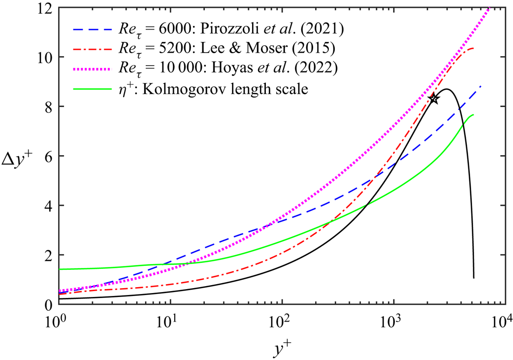
A comparison of the radial resolution  $\Delta y^+$ between various high- $Re$ DNS data is shown in figure 16. The corresponding Kolmogorov scale $\eta ^+={\epsilon ^+_k}^{-1/4}$ is also included as a reference. Near the wall, $\Delta y^+$ for our simulation is smallest among all cases, and much smaller than $\eta ^+$. For our case, $\Delta y^+$ increases progressively with $y^+$ and then reaches the maximum at $r/R \approx 0.44$. For the whole radial direction, $\Delta y^+$ is smaller than that of Lee & Moser (Reference Lee and Moser2015). In addition, it is less than $1.5\eta ^+$, which, following standard practices, indicates that a sufficient amount of grid points are used.
Comparison of the grid resolution in radial direction  $\Delta r^+$ among different high- $Re$ simulations. The black solid line with a star denotes our $Re_\tau \approx 5200$ result.
The simulation was performed using 32 768 processors (Intel Xeon Platinum 8280) on the Frontera supercomputer at Texas Advanced Computing Center, and 16 384 processors (AMD EPYC 7702) on Nocona at Texas Tech University High Performance Computing Center. A total of approximately  $40{\rm \pi}$ simulation time in terms of convective time units ( $R/U_b$) after the transient period was collected for statistical averaging, which corresponds to approximately 500 000 steps with time step $\Delta t=2.5\times 10^{-4} R/U_b$.
Appendix B. Estimated uncertainties for one-point statistics
We explain briefly the approach employed to estimate the uncertainties in the mean velocity and Reynolds stress components of the DNS of the pipe flow. During the simulations, the time samples of the quantities contributing to statistical terms are averaged over the azimuthal ( $\theta$) and axial ( $z$) directions. To compute the central statistical moments, the temporal correlations between the spatially averaged quantities are preserved by, for instance, writing a Reynolds stress component as $\langle u'_r u'_z\rangle = \langle \overline {u_r u_z} -\bar {u}_r \bar {u}_z \rangle$, where overbar means averaging over $\theta$ and $z$. In practice, the sample-mean estimator (SME) is used to estimate $\langle a \rangle$ from a finite number of time series samples $\{a_i\}_{i=1}^n$, where $a_i=a(t_i)$ are equispaced time samples. The SME for $\langle a \rangle$ is defined as
 \begin{equation} \hat{\mu}_a:=\hat{\mathbb{E}}[a]=\frac{1}{n}\sum_{i=1}^n a_i , \end{equation}
where  $\hat {\mathbb {E}}[a]$ is the estimated expectation of $a$. Based on the central limit theorem, for a sufficiently large number of samples, the SME converges to the true expectation via a Gaussian distribution,
 \begin{equation} \hat{\mu}_a\sim \mathcal{N}(\mu_a,\sigma^2(\hat{\mu}_a) ). \end{equation}
To estimate  $\sigma (\hat {\mu }_a)$ and hence quantify the time-averaging uncertainty in $\hat {\mu }_a$, an analytical expression can be derived that depends on the autocorrelation of time series $a$ at different lags; see e.g. Oliver et al. (Reference Oliver, Malaya, Ulerich and Moser2014) and Rezaeiravesh et al. (Reference Rezaeiravesh, Xavier, Vinuesa, Yao, Hussain and Schlatter2022). To avoid inaccuracy in $\sigma (\hat {\mu }_a)$ due to the oscillations in the sample-estimated autocorrelations, especially at higher lags, an autoregressive model is first fitted to the samples $\{a_i\}_{i=1}^n$, which is then used to construct a smooth model for the autocorrelations. The details of the approach can be found in Oliver et al. (Reference Oliver, Malaya, Ulerich and Moser2014) and D. Xavier et al. (personal communication 2022). The main hyperparameters of this uncertainty quantification (UQ) approach are the order of the autoregressive model and the number of training lags when modelling the autocorrelation function (ACF). In the present study, the optimal values of these hyperparameters are chosen based on the sampling frequency of the data at each $Re$. All estimations of uncertainties have been performed using UQit (Rezaeiravesh, Vinuesa & Schlatter Reference Rezaeiravesh, Vinuesa and Schlatter2021).
Following the above approach, the uncertainty in the statistical moments of any order can be estimated accurately. However, there are various turbulence statistics that are defined as a combination of the exponents of various moments; for instance, consider the turbulence intensity, r.m.s. fluctuations, turbulent kinetic energy, and various terms in the transport equations of the Reynolds stress components. The uncertainty in such terms can be estimated by applying the approach described in Rezaeiravesh et al. (Reference Rezaeiravesh, Xavier, Vinuesa, Yao, Hussain and Schlatter2022). The main idea for estimating the uncertainty in a compound statistical term is to estimate the uncertainty in its constitutive statistical moments and also estimate the cross-covariance between the SMEs corresponding to them. Following this procedure, in the DNS database reported online in connection with the present study, all statistics are accompanied by an accurate estimation of the corresponding time-averaging uncertainty. An important aspect of this procedure is that for the statistics expressed in wall units, the uncertainty of the wall friction velocity is also taken into account. This means, for instance, that for  $\langle u'_r u'_z\rangle ^+$, the uncertainty of both $\langle u'_r u'_z\rangle$ and $\langle u_\tau \rangle ^2$ are considered applying a Monte-Carlo-based UQ forward problem, which does not require any linearization.
Table 4 summarizes the sampling interval and the total number of samples used for UQ for simulations at different  $Re_\tau$. Our investigation showed that for the collected samples, an autoregressive model of order $20$ along with the sample-estimated ACF at the first $20$ lags, for $Re_\tau =180$, $550$ and $1000$, and $40$ lags, for $Re_\tau =2000$ and $5200$, leads to accurate models for autocorrelation of various quantities. For low-order moments, using sample-estimated ACF at a higher number of lags, especially near the centre of the pipe, could lead to slightly more accurate models for ACF. However, the difference in the resulting estimated uncertainty is below $1\,\%$.
Summary of the sampling of the flow variables used in the UQ analyses.

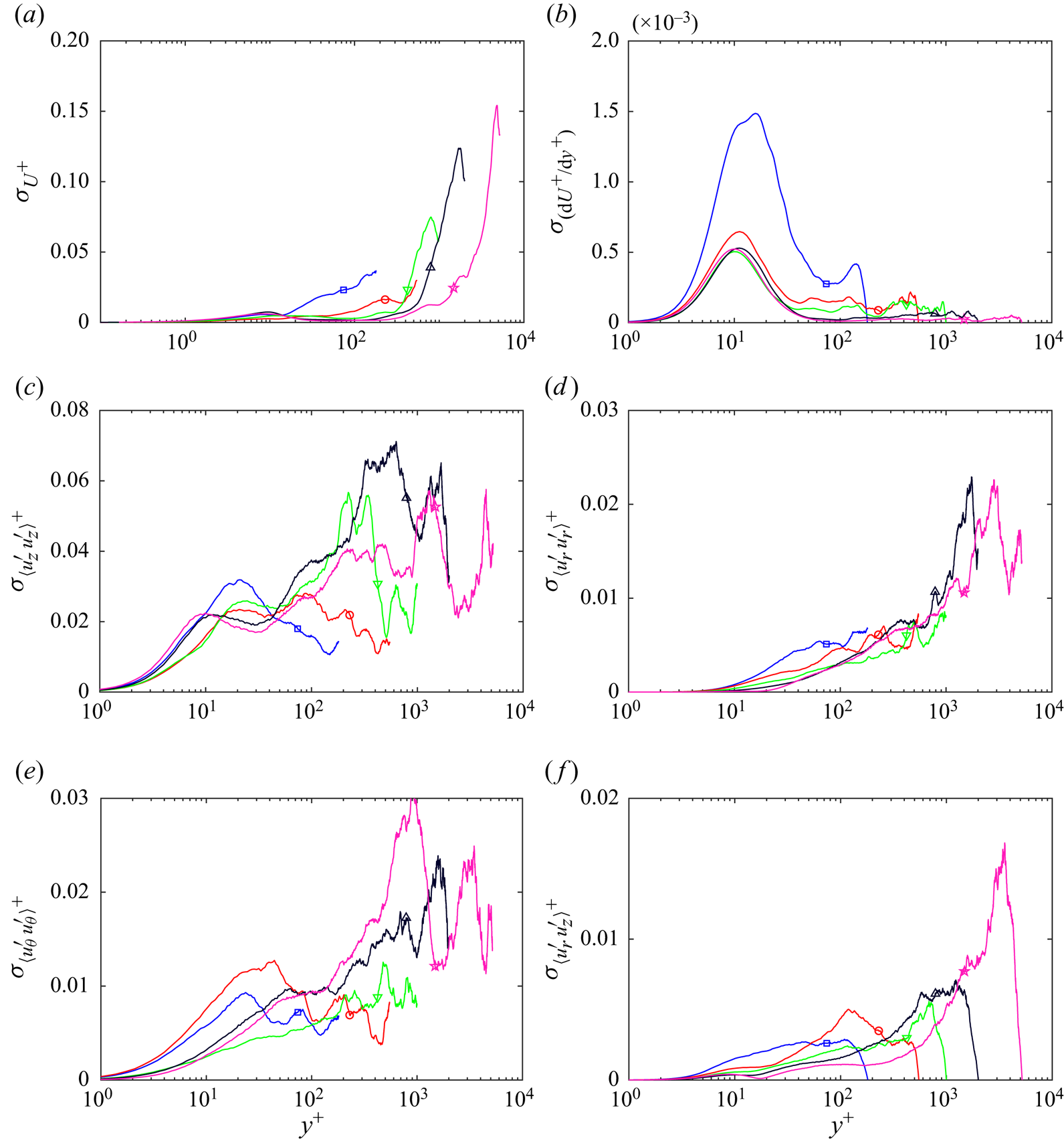
Figure 17 shows the standard deviation  $\sigma$ (see (B2)) of the sample estimation of different inner-scaled statistical terms. Clearly, the estimated uncertainties vary between the moments and also in the wall-normal direction. However, for all quantities, the lowest uncertainty (corresponding to highest certainty) is observed near the wall. Moreover, the estimated uncertainty for each quantity exhibits a similar variation in the wall-normal direction for different $Re_\tau$.
Estimated standard deviation of different statistical quantities: (a)  $U^+$, (b) $\partial U^+/\partial y^+$, (c) $\langle{u'^2_z}\rangle^{+}$, (d) $\langle{u'^2_r}\rangle^{+}$, (e) $\langle{u'^2_\theta}\rangle^{+}$, ( f) $\langle{u'_ru'_z}\rangle^{+}$.


 Open access

