

1 Introduction
We use standard notation ( $\mathbb {R}$
,
$\mathbb {R}$
, $\mathbb {C}$
for the real/complex numbers,
$\mathbb {C}$
for the real/complex numbers, $\mathbb {D}$
for the unit disk centered at the origin, etc). The Riemann sphere is denoted by
$\mathbb {D}$
for the unit disk centered at the origin, etc). The Riemann sphere is denoted by $\hat {\mathbb {C}}$
. The boundary (in
$\hat {\mathbb {C}}$
. The boundary (in $\mathbb {C}$
) of a set
$\mathbb {C}$
) of a set $X\subset \mathbb {C}$
is denoted by
$X\subset \mathbb {C}$
is denoted by $\mathrm {Bd}(X)$
. We consider only complex polynomials P; for such a P, let
$\mathrm {Bd}(X)$
. We consider only complex polynomials P; for such a P, let $J_P$
be its Julia set and
$J_P$
be its Julia set and $K_P$
be its filled Julia set. We normalize the circle so that its length is 1, and identify numbers of
$K_P$
be its filled Julia set. We normalize the circle so that its length is 1, and identify numbers of $[0, 1)$
with points on the circle and with the corresponding angles (so, we talk about the angle
$[0, 1)$
with points on the circle and with the corresponding angles (so, we talk about the angle $\frac 12$
rather than angle
$\frac 12$
rather than angle $\pi $
, etc). A chord is a closed straight line segment with endpoints on the unit circle
$\pi $
, etc). A chord is a closed straight line segment with endpoints on the unit circle $\mathbb {S}=\mathrm {Bd}(\mathbb {D})$
. The reader is referred to [Reference MilnorMil06, Reference Thurston and SchleicherThu85] for basic notions of complex polynomial dynamics on
$\mathbb {S}=\mathrm {Bd}(\mathbb {D})$
. The reader is referred to [Reference MilnorMil06, Reference Thurston and SchleicherThu85] for basic notions of complex polynomial dynamics on $\mathbb {C}$
, including Fatou and Julia sets, external rays, landing, etc.
$\mathbb {C}$
, including Fatou and Julia sets, external rays, landing, etc.
The connectedness locus $\mathcal {M}_d$
is the space of polynomials of degree d, up to affine conjugacy, with connected Julia sets. A fundamental problem is to understand the structure of
$\mathcal {M}_d$
is the space of polynomials of degree d, up to affine conjugacy, with connected Julia sets. A fundamental problem is to understand the structure of $\mathcal {M}_d$
. Major progress has been made for
$\mathcal {M}_d$
. Major progress has been made for $d=2$
, but much less is known for
$d=2$
, but much less is known for $d>2$
. Thurston [Reference Thurston and SchleicherThu85] introduced invariant laminations to provide a combinatorial model for
$d>2$
. Thurston [Reference Thurston and SchleicherThu85] introduced invariant laminations to provide a combinatorial model for $\mathcal {M}_2$
. A lamination
$\mathcal {M}_2$
. A lamination $\mathcal {L}$
is a compact set of chords, called leaves, that are pairwise disjoint in
$\mathcal {L}$
is a compact set of chords, called leaves, that are pairwise disjoint in $\mathbb {D}$
(equivalently, do not cross). Given a lamination
$\mathbb {D}$
(equivalently, do not cross). Given a lamination $\mathcal {L}$
, one can consider an equivalence relation
$\mathcal {L}$
, one can consider an equivalence relation $\sim _{\mathcal {L}}$
on
$\sim _{\mathcal {L}}$
on $\mathbb {S}$
where x,
$\mathbb {S}$
where x, $y\in \mathbb {S}$
are equivalent if there is a finite chain of leaves of
$y\in \mathbb {S}$
are equivalent if there is a finite chain of leaves of $\mathcal {L}$
connecting x and y. If all
$\mathcal {L}$
connecting x and y. If all $\sim _{\mathcal {L}}$
-classes of equivalence are finite and all leaves of
$\sim _{\mathcal {L}}$
-classes of equivalence are finite and all leaves of $\mathcal {L}$
are edges of their convex hulls, then we say that
$\mathcal {L}$
are edges of their convex hulls, then we say that $\mathcal {L}$
is a q-lamination.
$\mathcal {L}$
is a q-lamination.
Thurston constructs the quadratic minor lamination ( $\mathrm {QML}$
) whose leaves tag all invariant quadratic laminations (for
$\mathrm {QML}$
) whose leaves tag all invariant quadratic laminations (for $d\ge 2$
, a lamination is invariant if it is invariant under the map
$d\ge 2$
, a lamination is invariant if it is invariant under the map $\sigma _d(z)=z^d$
restricted to
$\sigma _d(z)=z^d$
restricted to $\mathbb {S}$
, see Definition 2.6). He shows that
$\mathbb {S}$
, see Definition 2.6). He shows that $\mathrm {QML}$
is a q-lamination; moreover, the quotient space
$\mathrm {QML}$
is a q-lamination; moreover, the quotient space $\mathcal {M}_2^{\mathrm {Comb}}=\mathbb {S}/\mathrm {QML}$
of the unit circle
$\mathcal {M}_2^{\mathrm {Comb}}=\mathbb {S}/\mathrm {QML}$
of the unit circle $\mathbb {S}$
by the equivalence relation defined by
$\mathbb {S}$
by the equivalence relation defined by $\mathrm {QML}$
is a monotone image of
$\mathrm {QML}$
is a monotone image of $\mathrm {Bd}(\mathcal {M}_2)$
(conjecturally, this map is a homeomorphism), cf. [Reference Thurston and SchleicherThu85, Reference Schleicher and SchleicherSch09]. No such models exist for
$\mathrm {Bd}(\mathcal {M}_2)$
(conjecturally, this map is a homeomorphism), cf. [Reference Thurston and SchleicherThu85, Reference Schleicher and SchleicherSch09]. No such models exist for $d>2$
.
$d>2$
.
A natural next object of study is $\mathcal {M}_3$
, that is, the space of all cubic polynomials with connected Julia sets, or its subspaces. Notice that polynomials from
$\mathcal {M}_3$
, that is, the space of all cubic polynomials with connected Julia sets, or its subspaces. Notice that polynomials from $\mathcal {M}_3$
are associated, in a natural fashion, with invariant cubic laminations. Similarly to the quadratic case, one can expect that to provide a model for a subspace of
$\mathcal {M}_3$
are associated, in a natural fashion, with invariant cubic laminations. Similarly to the quadratic case, one can expect that to provide a model for a subspace of $\mathcal {M}_3$
, one may need to describe the appropriate subspace of cubic laminations. We adopt this approach in a series of papers in which we consider symmetric cubic polynomials
$\mathcal {M}_3$
, one may need to describe the appropriate subspace of cubic laminations. We adopt this approach in a series of papers in which we consider symmetric cubic polynomials $P(z)=z^3+\unicode{x3bb} ^2 z$
with connected Julia sets; these form the cubic symmetric connected locus denoted by
$P(z)=z^3+\unicode{x3bb} ^2 z$
with connected Julia sets; these form the cubic symmetric connected locus denoted by $\mathcal M_{3,s}$
(see Figure 1).
$\mathcal M_{3,s}$
(see Figure 1).
The parameter space of symmetric cubic polynomials $\mathcal M_{3,s}$
.
$\mathcal M_{3,s}$
.

It is easy to see that the natural association between polynomials from $\mathcal M_{3,s}$
and their laminations leads to the space of all cubic invariant symmetric laminations defined as cubic invariant laminations that are also invariant under the map that sends each leaf
$\mathcal M_{3,s}$
and their laminations leads to the space of all cubic invariant symmetric laminations defined as cubic invariant laminations that are also invariant under the map that sends each leaf $\ell $
to the leaf
$\ell $
to the leaf $-\ell $
(that is, under the rotation of the unit circle by the angle
$-\ell $
(that is, under the rotation of the unit circle by the angle $\pi $
). In [Reference Blokh, Oversteegen, Selinger, Timorin and VejandlaBOSTV1], we define the ‘parametric’ q-lamination
$\pi $
). In [Reference Blokh, Oversteegen, Selinger, Timorin and VejandlaBOSTV1], we define the ‘parametric’ q-lamination $C_sCL$
(this stands for cubic symmetric comajor lamination) together with the induced factor space
$C_sCL$
(this stands for cubic symmetric comajor lamination) together with the induced factor space $\mathbb {S}/C_sCL$
of the unit circle
$\mathbb {S}/C_sCL$
of the unit circle $\mathbb {S}$
. This lamination parameterizes all cubic invariant symmetric laminations similar to how
$\mathbb {S}$
. This lamination parameterizes all cubic invariant symmetric laminations similar to how $\mathrm {QML}$
parameterizes all quadratic invariant laminations. Then, in [Reference Blokh, Oversteegen, Selinger, Timorin and VejandlaBOSTV3], we verify that
$\mathrm {QML}$
parameterizes all quadratic invariant laminations. Then, in [Reference Blokh, Oversteegen, Selinger, Timorin and VejandlaBOSTV3], we verify that $\mathbb {S}/C_sCL$
is a monotone model of
$\mathbb {S}/C_sCL$
is a monotone model of $\mathcal M_{3,s}$
.
$\mathcal M_{3,s}$
.
The present paper is devoted to the construction of $C_sCL$
and aims at understanding its structure and at obtaining suitable pictures of it. To this end, we obtain two main results. We state them here in §1 to make reading more focused and purposeful (we thank the referee for this suggestion).
$C_sCL$
and aims at understanding its structure and at obtaining suitable pictures of it. To this end, we obtain two main results. We state them here in §1 to make reading more focused and purposeful (we thank the referee for this suggestion).
Let us normalize the circle length to $1$
. For each chord
$1$
. For each chord $\ell =\overline {ab}$
, let
$\ell =\overline {ab}$
, let $|\ell |$
be the length of the shorter of the two circle arcs with endpoints a and b. Let c be a non-degenerate chord of length at most
$|\ell |$
be the length of the shorter of the two circle arcs with endpoints a and b. Let c be a non-degenerate chord of length at most $\frac 16$
. It is easy to see that there are two chords
$\frac 16$
. It is easy to see that there are two chords $M_c$
and
$M_c$
and $M^{\prime }_c$
that are disjoint, have the same
$M^{\prime }_c$
that are disjoint, have the same $\sigma _3$
-image as c, and have lengths at least
$\sigma _3$
-image as c, and have lengths at least $\frac 16$
. Denote by
$\frac 16$
. Denote by $\mathcal {S}(M_c)$
the component of
$\mathcal {S}(M_c)$
the component of $\mathbb {D}\setminus (M_c\cup M^{\prime }_c)$
that contains both
$\mathbb {D}\setminus (M_c\cup M^{\prime }_c)$
that contains both $M_c$
and
$M_c$
and $M^{\prime }_c$
in its boundary. Non-degenerate chords
$M^{\prime }_c$
in its boundary. Non-degenerate chords $\{c, -c\}$
of length at most
$\{c, -c\}$
of length at most $\frac 16$
such that the chords from the
$\frac 16$
such that the chords from the $\sigma _3$
-orbits of c and
$\sigma _3$
-orbits of c and $-c$
do not cross and never enter the set
$-c$
do not cross and never enter the set $\mathcal {S}(M_c)\cup -\mathcal {S}(M_c)$
form a legal pair (see Definition 3.18). A chord c such that
$\mathcal {S}(M_c)\cup -\mathcal {S}(M_c)$
form a legal pair (see Definition 3.18). A chord c such that $\{c, -c\}$
is a legal pair is said to be a comajor.
$\{c, -c\}$
is a legal pair is said to be a comajor.
The lamination $C_sCL$
is formed by all legal pairs and is in fact a q-lamination [Reference Blokh, Oversteegen, Selinger, Timorin and VejandlaBOSTV1]. Consider a special subset of
$C_sCL$
is formed by all legal pairs and is in fact a q-lamination [Reference Blokh, Oversteegen, Selinger, Timorin and VejandlaBOSTV1]. Consider a special subset of $C_sCL$
that consists of co-periodic comajors (a leaf is co-periodic if it is not periodic but its image is). In the first main result of the paper, Theorem 4.15, we show that co-periodic comajors are dense in the entire
$C_sCL$
that consists of co-periodic comajors (a leaf is co-periodic if it is not periodic but its image is). In the first main result of the paper, Theorem 4.15, we show that co-periodic comajors are dense in the entire $C_sCL$
. To state our second main result we need some definitions.
$C_sCL$
. To state our second main result we need some definitions.
A $2n$
-periodic point x of
$2n$
-periodic point x of $\sigma _3$
with
$\sigma _3$
with $\sigma _3^n(x)=-x$
is said to be of type B. All other periodic points of
$\sigma _3^n(x)=-x$
is said to be of type B. All other periodic points of $\sigma _3$
are said to be of type D. For example,
$\sigma _3$
are said to be of type D. For example, $\frac 14$
is a periodic point of type B, while
$\frac 14$
is a periodic point of type B, while ${1}/{26}$
is a periodic point of type D. Our choice of symbols B and D for the types of periodic orbits follows Milnor’s notation for polynomial hyperbolic components and stands for Bi-transitive and Disjoint, respectively. A periodic leaf of a symmetric lamination is of type B if its endpoints are of type B, and of type D if its endpoints are of type D. By Lemma 5.9, all periodic leaves of symmetric laminations are of type B or of type D. A co-periodic leaf of a symmetric lamination is of type B if its image is a periodic leaf of type B, and of type D otherwise. A periodic point (leaf) of type B and period
${1}/{26}$
is a periodic point of type D. Our choice of symbols B and D for the types of periodic orbits follows Milnor’s notation for polynomial hyperbolic components and stands for Bi-transitive and Disjoint, respectively. A periodic leaf of a symmetric lamination is of type B if its endpoints are of type B, and of type D if its endpoints are of type D. By Lemma 5.9, all periodic leaves of symmetric laminations are of type B or of type D. A co-periodic leaf of a symmetric lamination is of type B if its image is a periodic leaf of type B, and of type D otherwise. A periodic point (leaf) of type B and period $2n$
has lock period n; so,
$2n$
has lock period n; so, $\frac 14$
is a periodic point of period 2 but of block period 1. A periodic point (leaf) of type D and period n has block period n; so,
$\frac 14$
is a periodic point of period 2 but of block period 1. A periodic point (leaf) of type D and period n has block period n; so, ${1}/{26}$
is a periodic point of period 3 and block period 3. A co-periodic leaf is said to be of block period n if its image is of block period n.
${1}/{26}$
is a periodic point of period 3 and block period 3. A co-periodic leaf is said to be of block period n if its image is of block period n.
Given a chord $\ell =\overline {ab}$
with
$\ell =\overline {ab}$
with $|\ell |<\frac 12$
, set
$|\ell |<\frac 12$
, set $H(\ell )$
to be a circle arc of length
$H(\ell )$
to be a circle arc of length $|\ell |$
with endpoints a and b. If
$|\ell |$
with endpoints a and b. If $\ell $
and
$\ell $
and $\ell '$
are chords disjoint inside
$\ell '$
are chords disjoint inside $\mathbb {D}$
with
$\mathbb {D}$
with $H(\ell ')\subset H(\ell )$
, then we write
$H(\ell ')\subset H(\ell )$
, then we write $\ell '\prec \ell $
. Suppose that co-periodic comajors c and
$\ell '\prec \ell $
. Suppose that co-periodic comajors c and $c'$
are such that
$c'$
are such that $c'\prec c$
, both c and
$c'\prec c$
, both c and $c'$
are either of type B or type D, and c and
$c'$
are either of type B or type D, and c and $c'$
have the same block period n. In Theorem 5.13, we prove that then there exists a co-periodic comajor d with
$c'$
have the same block period n. In Theorem 5.13, we prove that then there exists a co-periodic comajor d with $c'\prec d\prec c$
such that d is of block period
$c'\prec d\prec c$
such that d is of block period $j<n$
. This yields an algorithm allowing one to inductively construct the family of all co-periodic comajors (dense in
$j<n$
. This yields an algorithm allowing one to inductively construct the family of all co-periodic comajors (dense in $C_sCL$
as we know). We call it the L-algorithm.
$C_sCL$
as we know). We call it the L-algorithm.
The L-algorithm is similar to the famous Lavaurs algorithm [Reference LavaursLav86, Reference LavaursLav89] that defines a dense (in $\mathrm {QML}$
) set of pairwise disjoint
$\mathrm {QML}$
) set of pairwise disjoint $\sigma _2$
-periodic chords. The co-periodic comajors play for
$\sigma _2$
-periodic chords. The co-periodic comajors play for $C_sCL$
the same role as the periodic minors for
$C_sCL$
the same role as the periodic minors for $\mathrm {QML}$
. In a nutshell, the L-algorithm is as follows. Start with marking the co-periodic comajors of block period 1, namely, the chords
$\mathrm {QML}$
. In a nutshell, the L-algorithm is as follows. Start with marking the co-periodic comajors of block period 1, namely, the chords
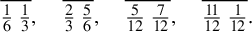 $$ \begin{align*} \overline{\tfrac{1}{6}\,\tfrac{1}{3}},\quad \overline{\tfrac{2}{3}\,\tfrac{5}{6}},\quad \overline{\tfrac{5}{12}\,\tfrac{7}{12}},\quad \overline{\tfrac{11}{12}\,\tfrac{1}{12}}. \end{align*} $$
Of these four leaves, the first two are of type D, and the last two are of type B, cf. Figure 2. Once all co-periodic comajors of block periods from 1 to $k-1$
are constructed, generate those of block period k as follows. Mark all type-D points of preperiod 1 and block period k. Next, connect these points consecutively while bypassing the already generated leaves. Similarly, mark type-B points of block period k and connect them. Every time there is a choice between longer connections and shorter ones, the latter must be preferred. Details are given in Theorem 5.13.
$k-1$
are constructed, generate those of block period k as follows. Mark all type-D points of preperiod 1 and block period k. Next, connect these points consecutively while bypassing the already generated leaves. Similarly, mark type-B points of block period k and connect them. Every time there is a choice between longer connections and shorter ones, the latter must be preferred. Details are given in Theorem 5.13.
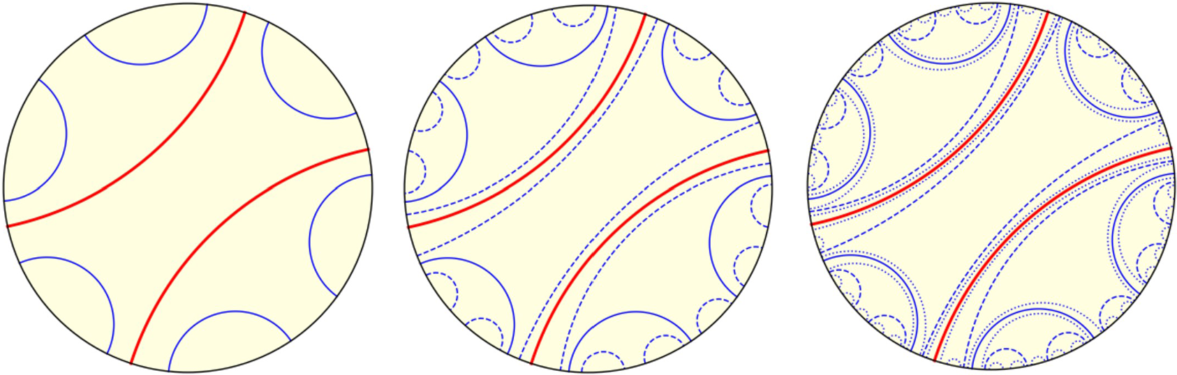
Three initial steps in the construction of the symmetric cubic comajor lamination $C_sCL$
. Boldface curves indicate leaves of block period 1 constructed in the first step, normal thickness leaves are leaves of block period 2 constructed in the second step, and the dotted leaves are of block period 3 constructed in the third step. Darker leaves are co-periodic comajors of type B, lighter leaves are co-periodic comajors of type D.
$C_sCL$
. Boldface curves indicate leaves of block period 1 constructed in the first step, normal thickness leaves are leaves of block period 2 constructed in the second step, and the dotted leaves are of block period 3 constructed in the third step. Darker leaves are co-periodic comajors of type B, lighter leaves are co-periodic comajors of type D.
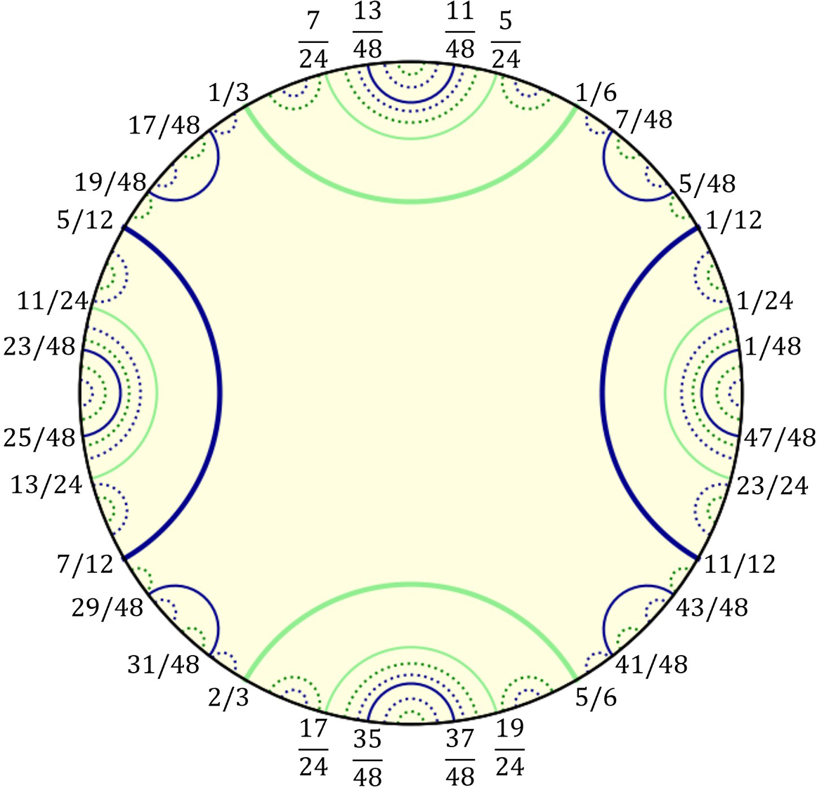
Figure 2 shows the three initial steps of the construction.
The L-algorithm defines an involution on the family of all co-periodic comajors reminiscent of the quadratic case and the title of Lavaurs’ paper [Reference LavaursLav86] (we thank the referee for bringing this to our attention).
Now we would like to address the issue of the tools used in the paper. We follow Thurston’s approach, implemented so successfully in his seminal preprint that started circulating in 1985 and was, in our view, a key step in the development of polynomial dynamics. We were influenced by it, and decided to apply similar ideas to cubic symmetric polynomials. Thus, our choice here was partially a matter of taste. Another reason for not using analytic machinery when constructing a model space for $\mathcal M_{3,s}$
was that while Thurston’s approach is involved, it is also elementary and, for this reason, can be potentially accessible to a wider audience. Finally, combining analytic and combinatorial methods in one construction seems to us less attractive and elegant as it is less structured and requires going back and forth between different methods. This explains the choice of techniques.
$\mathcal M_{3,s}$
was that while Thurston’s approach is involved, it is also elementary and, for this reason, can be potentially accessible to a wider audience. Finally, combining analytic and combinatorial methods in one construction seems to us less attractive and elegant as it is less structured and requires going back and forth between different methods. This explains the choice of techniques.
The paper is organized as follows. We discuss laminations in §2. In §3, we consider general results and concepts concerning symmetric laminations introduced in [Reference Blokh, Oversteegen, Selinger, Timorin and VejandlaBOSTV1]. In §4, we state a few specific properties of the space $C_sCL$
and use them, and additional arguments, to verify the Fatou conjecture about the density of hyperbolicity for symmetric cubic laminations. More precisely, observe that co-periodic comajors correspond to periodic majors; in §4, we associate them with q-laminations with periodic Fatou gaps of degree greater than 1 and show that these are dense. Finally, in §5, we describe and justify the L-algorithm similar to the Lavaurs algorithm.
$C_sCL$
and use them, and additional arguments, to verify the Fatou conjecture about the density of hyperbolicity for symmetric cubic laminations. More precisely, observe that co-periodic comajors correspond to periodic majors; in §4, we associate them with q-laminations with periodic Fatou gaps of degree greater than 1 and show that these are dense. Finally, in §5, we describe and justify the L-algorithm similar to the Lavaurs algorithm.
2 Laminations: classical definitions
Identify $\mathbb {S}$
with
$\mathbb {S}$
with $\mathbb {R}/\mathbb {Z}$
and define the map
$\mathbb {R}/\mathbb {Z}$
and define the map $\sigma _d:\mathbb {S} \rightarrow \mathbb {S}$
for
$\sigma _d:\mathbb {S} \rightarrow \mathbb {S}$
for $d \geq 2$
as
$d \geq 2$
as $\sigma _d(z)=dz \mod 1$
; clearly,
$\sigma _d(z)=dz \mod 1$
; clearly, $\sigma _d$
is locally one-to-one on
$\sigma _d$
is locally one-to-one on $\mathbb {S}$
. A monic (that is, with leading coefficient 1) complex polynomial P with locally connected Julia set
$\mathbb {S}$
. A monic (that is, with leading coefficient 1) complex polynomial P with locally connected Julia set $J_P$
gives rise to an equivalence relation
$J_P$
gives rise to an equivalence relation $\sim _P$
on
$\sim _P$
on $\mathbb {S}$
so that
$\mathbb {S}$
so that $x \sim _P y$
if and only if the external rays of arguments x and y land at the same point of
$x \sim _P y$
if and only if the external rays of arguments x and y land at the same point of $J_P$
. Equivalence classes of
$J_P$
. Equivalence classes of $\sim _P$
have pairwise disjoint convex hulls. The topological Julia set
$\sim _P$
have pairwise disjoint convex hulls. The topological Julia set $\mathbb {S}/\sim _P=J_{\sim _P}$
is homeomorphic to
$\mathbb {S}/\sim _P=J_{\sim _P}$
is homeomorphic to $J_P$
, and the topological polynomial
$J_P$
, and the topological polynomial $f_{\sim _P}:J_{\sim _P}\to J_{\sim _P}$
, induced by
$f_{\sim _P}:J_{\sim _P}\to J_{\sim _P}$
, induced by $\sigma _d$
, is topologically conjugate to
$\sigma _d$
, is topologically conjugate to $P|_{J_P}$
.
$P|_{J_P}$
.
An equivalence relation $\sim $
on
$\sim $
on $\mathbb {S}$
, with similar properties to those of
$\mathbb {S}$
, with similar properties to those of $\sim _P$
above, can be introduced with no reference to complex polynomials.
$\sim _P$
above, can be introduced with no reference to complex polynomials.
Definition 2.1. (Laminational equivalence relation)
An equivalence relation $\sim $
on the unit circle
$\sim $
on the unit circle $\mathbb {S}$
is called a laminational equivalence relation if it has the following properties:
$\mathbb {S}$
is called a laminational equivalence relation if it has the following properties:
(E1) the graph of $\sim $
is a closed subset in
$\sim $
is a closed subset in $\mathbb {S} \times \mathbb {S}$
;
$\mathbb {S} \times \mathbb {S}$
;
(E2) convex hulls of distinct equivalence classes are disjoint;
(E3) each equivalence class of $\sim $
is finite.
$\sim $
is finite.
For a closed set $A\subset \mathbb {S}$
, we denote its convex hull by
$A\subset \mathbb {S}$
, we denote its convex hull by $\mathrm {CH}(A)$
. An edge of
$\mathrm {CH}(A)$
. An edge of $\mathrm {CH}(A)$
is a chord of
$\mathrm {CH}(A)$
is a chord of $\mathbb {S}$
contained in the boundary of
$\mathbb {S}$
contained in the boundary of $\mathrm {CH}(A)$
. Given points a,
$\mathrm {CH}(A)$
. Given points a, $b\in \mathbb {S}$
, let
$b\in \mathbb {S}$
, let $(a,b)$
be the positively oriented arc in
$(a,b)$
be the positively oriented arc in $\mathbb {S}$
from a to b and let
$\mathbb {S}$
from a to b and let $\overline {ab}$
be the chord with endpoints a and b.
$\overline {ab}$
be the chord with endpoints a and b.
Definition 2.2. (Invariance)
A laminational equivalence relation $\sim $
is (
$\sim $
is ( $\sigma _d$
-)invariant if:
$\sigma _d$
-)invariant if:
(I1) $\sim $
is forward invariant: for a class
$\sim $
is forward invariant: for a class $\mathbf {g}$
, the set
$\mathbf {g}$
, the set $\sigma _d(\mathbf {g})$
is a class too;
$\sigma _d(\mathbf {g})$
is a class too;
(I2) $\sim $
is backward invariant: for a class
$\sim $
is backward invariant: for a class $\mathbf {g}$
, its pre-image
$\mathbf {g}$
, its pre-image $\sigma _d^{-1}(\mathbf {g})=\{x\in \mathbb {S}: \sigma _d(x)\in \mathbf {g}\}$
is a union of classes;
$\sigma _d^{-1}(\mathbf {g})=\{x\in \mathbb {S}: \sigma _d(x)\in \mathbf {g}\}$
is a union of classes;
(I3) for any $\sim $
-class
$\sim $
-class $\mathbf {g}$
with more than two points, the map
$\mathbf {g}$
with more than two points, the map $\sigma _d|_{\mathbf {g}}: \mathbf {g}\to \sigma _d(\mathbf {g})$
is a covering map with positive orientation, that is, for every connected component
$\sigma _d|_{\mathbf {g}}: \mathbf {g}\to \sigma _d(\mathbf {g})$
is a covering map with positive orientation, that is, for every connected component $(s, t)$
of
$(s, t)$
of $\mathbb {S}\setminus \mathbf {g}$
, the arc in the circle
$\mathbb {S}\setminus \mathbf {g}$
, the arc in the circle $(\sigma _d(s), \sigma _d(t))$
is a connected component of
$(\sigma _d(s), \sigma _d(t))$
is a connected component of $\mathbb {S}\setminus \sigma _d(\mathbf {g})$
.
$\mathbb {S}\setminus \sigma _d(\mathbf {g})$
.
Definition 2.3. A lamination $\mathcal {L}$
is a set of chords in the closed unit disk
$\mathcal {L}$
is a set of chords in the closed unit disk $\overline {\mathbb {D}}$
, called leaves of
$\overline {\mathbb {D}}$
, called leaves of $\mathcal {L}$
, if it satisfies the following conditions:
$\mathcal {L}$
, if it satisfies the following conditions:
(L1) leaves of $\mathcal {L}$
do not cross; (L2) the set
$\mathcal {L}$
do not cross; (L2) the set $\mathcal {L}^{\ast }=\bigcup _{\ell \in \mathcal {L}}\ell $
is closed.
$\mathcal {L}^{\ast }=\bigcup _{\ell \in \mathcal {L}}\ell $
is closed.
If condition (L2) is not assumed, then $\mathcal {L}$
is called a prelamination.
$\mathcal {L}$
is called a prelamination.
A degenerate leaf is a point of $\mathbb {S}$
. Given a leaf
$\mathbb {S}$
. Given a leaf $\ell =\overline {ab}\in \mathcal {L}$
, let
$\ell =\overline {ab}\in \mathcal {L}$
, let $\sigma _d(\ell )$
be the chord with endpoints
$\sigma _d(\ell )$
be the chord with endpoints $\sigma _d(a)$
and
$\sigma _d(a)$
and $\sigma _d(b)$
; then,
$\sigma _d(b)$
; then, $\ell $
is called a pullback of
$\ell $
is called a pullback of $\sigma _d(\ell )$
. If
$\sigma _d(\ell )$
. If $a\ne b$
but
$a\ne b$
but $\sigma _d(a) = \sigma _d(b)$
, call
$\sigma _d(a) = \sigma _d(b)$
, call $\ell $
a critical leaf. Let
$\ell $
a critical leaf. Let $\sigma _d^{\ast }:\mathcal {L}^{\ast }\rightarrow \overline {\mathbb {D}}$
be the linear extension of
$\sigma _d^{\ast }:\mathcal {L}^{\ast }\rightarrow \overline {\mathbb {D}}$
be the linear extension of $\sigma _d$
over all the leaves in
$\sigma _d$
over all the leaves in $\mathcal {L}$
. Then,
$\mathcal {L}$
. Then, $\sigma _d^{\ast }$
is continuous and
$\sigma _d^{\ast }$
is continuous and $\sigma _d^{\ast }$
is one-to-one on any non-critical leaf. If
$\sigma _d^{\ast }$
is one-to-one on any non-critical leaf. If $\mathcal {L}$
includes all points of
$\mathcal {L}$
includes all points of $\mathbb {S}$
as degenerate leaves, then
$\mathbb {S}$
as degenerate leaves, then $\mathcal {L}^{\ast }$
is a continuum.
$\mathcal {L}^{\ast }$
is a continuum.
Definition 2.4. (Gap)
A gap G of a lamination $\mathcal {L}$
is the closure of a component of
$\mathcal {L}$
is the closure of a component of $\mathbb {D}\setminus \mathcal {L}^{\ast }$
; its boundary leaves are called edges (of the gap).
$\mathbb {D}\setminus \mathcal {L}^{\ast }$
; its boundary leaves are called edges (of the gap).
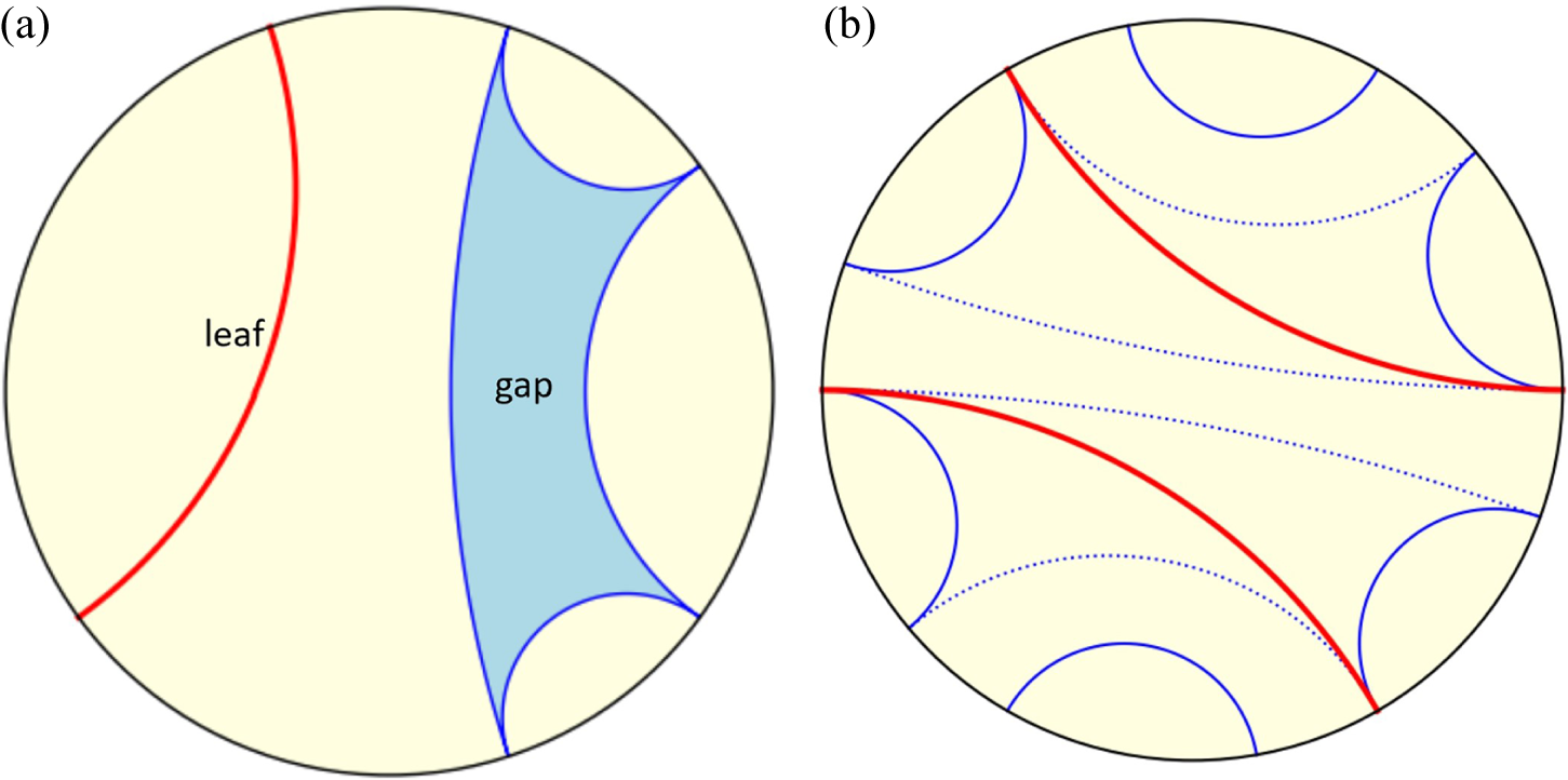
Figure 3 illustrates these notions. If G is a leaf/gap of $\mathcal {L}$
, then G equals the convex hull of
$\mathcal {L}$
, then G equals the convex hull of $G\cap \mathbb {S}$
. If G is a leaf or a gap of
$G\cap \mathbb {S}$
. If G is a leaf or a gap of $\mathcal {L}$
, we let
$\mathcal {L}$
, we let $\sigma _d(G)$
be the convex hull of
$\sigma _d(G)$
be the convex hull of $\sigma _d(G\cap \mathbb {S})$
. Notice that
$\sigma _d(G\cap \mathbb {S})$
. Notice that $\mathrm {Bd}(G) \cap \mathbb {S} = G \cap \mathbb {S}$
. Points of
$\mathrm {Bd}(G) \cap \mathbb {S} = G \cap \mathbb {S}$
. Points of $G\cap \mathbb {S}$
are called the vertices of G. A gap G is called infinite (finite) if and only if
$G\cap \mathbb {S}$
are called the vertices of G. A gap G is called infinite (finite) if and only if $G\cap \mathbb {S}$
is infinite (finite). A gap G is called a triangular gap if
$G\cap \mathbb {S}$
is infinite (finite). A gap G is called a triangular gap if $G\cap \mathbb {S}$
consists of three points.
$G\cap \mathbb {S}$
consists of three points.
(a) A gap and a leaf. (b) Long pullbacks (dotted) versus short pullbacks (solid).
Definition 2.5. Let $\mathcal {L}$
be a lamination. The equivalence relation
$\mathcal {L}$
be a lamination. The equivalence relation $\sim _{\mathcal {L}}$
on
$\sim _{\mathcal {L}}$
on $\mathbb {S}$
induced by
$\mathbb {S}$
induced by $\mathcal {L}$
is defined by declaring that
$\mathcal {L}$
is defined by declaring that $x\sim _{\mathcal {L}} y$
if and only if there exists a finite concatenation of leaves of
$x\sim _{\mathcal {L}} y$
if and only if there exists a finite concatenation of leaves of $\mathcal {L}$
joining x to y.
$\mathcal {L}$
joining x to y.
Definition 2.6. (Invariant (pre)laminations)
A (pre)lamination $\mathcal {L}$
is (
$\mathcal {L}$
is ( $\sigma _d$
-)invariant if:
$\sigma _d$
-)invariant if:
(D1) $\mathcal {L}$
is forward invariant. For each
$\mathcal {L}$
is forward invariant. For each $\ell \in \mathcal {L}$
, either
$\ell \in \mathcal {L}$
, either $\sigma _d(\ell ) \in \mathcal {L}$
or
$\sigma _d(\ell ) \in \mathcal {L}$
or $\sigma _d(\ell )$
is a point in
$\sigma _d(\ell )$
is a point in $\mathbb {S}$
; and
$\mathbb {S}$
; and
(D2) $\mathcal {L}$
is backward invariant.
$\mathcal {L}$
is backward invariant.
-
(1) For each $\ell \in \mathcal {L}$
, there exists a leaf
$\ell ' \in \mathcal {L}$
such that
$\sigma _d(\ell ')=\ell $
.
$\ell \in \mathcal {L}$
, there exists a leaf
$\ell ' \in \mathcal {L}$
such that
$\sigma _d(\ell ')=\ell $
. -
(2) For each
$\ell \in \mathcal {L}$
such that
$\sigma _d(\ell )$
is a non-degenerate leaf, there exists d disjoint leaves
$\ell _1$
,…,
$\ell _d$
in
$\mathcal {L}$
such that
$\ell = \ell _1$
and
$\sigma _d(\ell _i)=\sigma _d(\ell )$
for all i.


Definition 2.7. (q-lamination)
A lamination $\mathcal {L}$
is called a q-lamination if the equivalence relation
$\mathcal {L}$
is called a q-lamination if the equivalence relation $\sim _{\mathcal {L}}$
is laminational and
$\sim _{\mathcal {L}}$
is laminational and $\mathcal {L}$
consists of the edges of the convex hulls of
$\mathcal {L}$
consists of the edges of the convex hulls of $\sim _{\mathcal {L}}$
-classes.
$\sim _{\mathcal {L}}$
-classes.
Remark 2.8. Since a q-lamination $\mathcal {L}$
consists of edges of the
$\mathcal {L}$
consists of edges of the $\sim _{\mathcal {L}}$
classes, two leaves of
$\sim _{\mathcal {L}}$
classes, two leaves of $\mathcal {L}$
sharing an endpoint must be edges of a finite gap. Also, given a laminational equivalence relation
$\mathcal {L}$
sharing an endpoint must be edges of a finite gap. Also, given a laminational equivalence relation $\approx $
, we may consider the family of edges of convex hulls of
$\approx $
, we may consider the family of edges of convex hulls of $\approx $
-classes; this family is denoted by
$\approx $
-classes; this family is denoted by $\mathcal {L}_\approx $
and is called the lamination generated by
$\mathcal {L}_\approx $
and is called the lamination generated by $\approx $
. Evidently, such
$\approx $
. Evidently, such $\mathcal {L}_\approx $
is a q-lamination.
$\mathcal {L}_\approx $
is a q-lamination.
Definition 2.9. (Siblings)
Two chords are called siblings if they have the same image. Any d disjoint chords with the same non-degenerate image are called a sibling collection.
Definition 2.10. (Monotone map)
Let X, Y be topological spaces and $f:X\rightarrow Y$
be continuous. Then, f is said to be monotone if
$f:X\rightarrow Y$
be continuous. Then, f is said to be monotone if $f^{-1}(y)$
is connected for each
$f^{-1}(y)$
is connected for each $y \in Y$
. It is known that if f is monotone and X is a continuum, then
$y \in Y$
. It is known that if f is monotone and X is a continuum, then $f^{-1}(Z)$
is connected for every connected
$f^{-1}(Z)$
is connected for every connected $Z\subset f(X)$
.
$Z\subset f(X)$
.
Definition 2.11. (Gap-invariance)
A lamination $\mathcal {L}$
is gap invariant if for each gap G, the set
$\mathcal {L}$
is gap invariant if for each gap G, the set $\sigma _d(G)$
is a gap, or a leaf, or a single point. In the first case, we also require that
$\sigma _d(G)$
is a gap, or a leaf, or a single point. In the first case, we also require that $\sigma _d^*|_{\mathrm {Bd}(G)}:\mathrm {Bd}(G)\to \mathrm {Bd}(\sigma _d(G))$
maps as the composition of a monotone map and a covering map to the boundary of the image gap, with positive orientation (that is, as you move through the vertices of G in a clockwise direction around
$\sigma _d^*|_{\mathrm {Bd}(G)}:\mathrm {Bd}(G)\to \mathrm {Bd}(\sigma _d(G))$
maps as the composition of a monotone map and a covering map to the boundary of the image gap, with positive orientation (that is, as you move through the vertices of G in a clockwise direction around $\mathrm {Bd}(G)$
, their corresponding images in
$\mathrm {Bd}(G)$
, their corresponding images in $\sigma _d(G)$
must also be aligned clockwise in
$\sigma _d(G)$
must also be aligned clockwise in $\mathrm {Bd}(\sigma _d(G))$
).
$\mathrm {Bd}(\sigma _d(G))$
).
Definition 2.12. (Degree)
The degree of the map $\sigma _d^*|_{\mathrm {Bd}(G)}:\mathrm {Bd}(G)\to \mathrm {Bd}(\sigma _d(G))$
, or of the gap G, is defined as the number of components of
$\sigma _d^*|_{\mathrm {Bd}(G)}:\mathrm {Bd}(G)\to \mathrm {Bd}(\sigma _d(G))$
, or of the gap G, is defined as the number of components of $(\sigma _d^*)^{-1}(x)$
in
$(\sigma _d^*)^{-1}(x)$
in $\mathrm {Bd}(G)$
, for any
$\mathrm {Bd}(G)$
, for any ${x\in \mathrm {Bd}(\sigma _d(G))}$
. In other words, if every leaf of
${x\in \mathrm {Bd}(\sigma _d(G))}$
. In other words, if every leaf of $\sigma _d(G)$
has k disjoint pre-image leaves in G, then the degree of the map
$\sigma _d(G)$
has k disjoint pre-image leaves in G, then the degree of the map $\sigma _d^*$
is k. A gap G is called a critical gap if
$\sigma _d^*$
is k. A gap G is called a critical gap if $k>1$
.
$k>1$
.
The following results are proved in [Reference Blokh, Mimbs, Oversteegen and ValkenburgBMOV13].
Theorem 2.13. Every ( $\sigma _d$
-)invariant lamination is gap invariant.
$\sigma _d$
-)invariant lamination is gap invariant.
Theorem 2.14. The closure of an invariant prelamination is an invariant lamination. The space of all $\sigma _d$
-invariant laminations is compact.
$\sigma _d$
-invariant laminations is compact.
3 Symmetric cubic comajor lamination: preliminaries
This section describes results of [Reference Blokh, Oversteegen, Selinger, Timorin and VejandlaBOSTV1]. From now on, normalize the circle so that its length is $1$
; the length of arcs and angles are measured accordingly. Given a chord
$1$
; the length of arcs and angles are measured accordingly. Given a chord $\ell =\overline {ab}$
, denote by
$\ell =\overline {ab}$
, denote by $-\ell $
the chord obtained by rotating
$-\ell $
the chord obtained by rotating $\ell $
by the angle
$\ell $
by the angle $\frac 12$
. Define the length
$\frac 12$
. Define the length $\|\overline {ab}\|$
of a chord
$\|\overline {ab}\|$
of a chord $\overline {ab}$
as the shorter of the lengths of the arcs in
$\overline {ab}$
as the shorter of the lengths of the arcs in $\mathbb {S}=\mathbb {R}/\mathbb {Z}$
with the endpoints a and b. The maximum length of a chord is
$\mathbb {S}=\mathbb {R}/\mathbb {Z}$
with the endpoints a and b. The maximum length of a chord is $\frac 12$
. Divide leaves into four categories by their length.
$\frac 12$
. Divide leaves into four categories by their length.
Definition 3.1. A short leaf is a leaf $\ell $
such that
$\ell $
such that $0<\|\ell \|<\tfrac 16$
, a medium leaf is a leaf
$0<\|\ell \|<\tfrac 16$
, a medium leaf is a leaf $\ell $
such that
$\ell $
such that $\tfrac 16\leq \|\ell \|<\tfrac 13$
, and a long leaf is a leaf
$\tfrac 16\leq \|\ell \|<\tfrac 13$
, and a long leaf is a leaf $\ell $
such that
$\ell $
such that $\tfrac 13<\|\ell \|\leq \tfrac 12$
. Critical leaves are leaves of length exactly
$\tfrac 13<\|\ell \|\leq \tfrac 12$
. Critical leaves are leaves of length exactly $\frac 13$
.
$\frac 13$
.
For brevity, we call a leaf $\ell $
long/medium if
$\ell $
long/medium if $\|\ell \|\ge \frac 16$
.
$\|\ell \|\ge \frac 16$
.
By Definition 2.9, we cannot talk about sibling collections that include critical leaves. However, it is clear that a non-critical leaf $\ell $
has siblings. Consider this issue in detail.
$\ell $
has siblings. Consider this issue in detail.
Lemma 3.2. [Reference Blokh, Oversteegen, Selinger, Timorin and VejandlaBOSTV1, Lemma 3.4]
The possibilities for leaves in a sibling collection are:
-
(sss) all leaves are short;
-
(mmm) all leaves are medium;
-
(sml) one leaf is short, one medium, and one long.
A sibling collection is completely determined by its type and one leaf.
These are general facts; let us now become more specific.
Definition 3.3. (Cubic symmetric lamination)
A $\sigma _3$
-invariant lamination
$\sigma _3$
-invariant lamination $\mathcal {L}$
is called a cubic symmetric lamination if:
$\mathcal {L}$
is called a cubic symmetric lamination if:
(D3) for each $\ell \in \mathcal {L}$
, we have
$\ell \in \mathcal {L}$
, we have $-\ell \in \mathcal {L}$
.
$-\ell \in \mathcal {L}$
.
Here, $-\ell $
denotes the result of the half-turn (rotation by 180 degrees) about the origin of
$-\ell $
denotes the result of the half-turn (rotation by 180 degrees) about the origin of $\mathbb {C}$
applied to
$\mathbb {C}$
applied to $\ell $
. Note: if the endpoints of
$\ell $
. Note: if the endpoints of $\ell $
have arguments
$\ell $
have arguments $\alpha $
and
$\alpha $
and $\beta $
, then the endpoints of
$\beta $
, then the endpoints of $-\ell $
have arguments
$-\ell $
have arguments $\alpha +\tfrac 12$
and
$\alpha +\tfrac 12$
and $\beta +\tfrac 12$
. Unless otherwise stated, let
$\beta +\tfrac 12$
. Unless otherwise stated, let $\mathcal {L}$
be a cubic symmetric lamination.
$\mathcal {L}$
be a cubic symmetric lamination.
Definition 3.4. Suppose that $\ell =\overline {ab}$
is a non-critical chord which is not a diameter and the arc
$\ell =\overline {ab}$
is a non-critical chord which is not a diameter and the arc $(a, b)$
is shorter than the arc
$(a, b)$
is shorter than the arc $(b, a)$
. Denote the chord
$(b, a)$
. Denote the chord $\overline {(a+\frac 13) (b-\frac 13)}$
by
$\overline {(a+\frac 13) (b-\frac 13)}$
by $\ell '$
and the chord
$\ell '$
and the chord $\overline {(a+\frac 23) (b-\frac 23)}$
by
$\overline {(a+\frac 23) (b-\frac 23)}$
by $\ell "$
.
$\ell "$
.
As $\sigma _3(\ell ')=\sigma _3(\ell ")=\sigma _3(\ell )$
, the chords
$\sigma _3(\ell ')=\sigma _3(\ell ")=\sigma _3(\ell )$
, the chords $\ell $
,
$\ell $
, $\ell '$
,
$\ell '$
, $\ell "$
form a sibling collection. For a long/medium non-critical leaf
$\ell "$
form a sibling collection. For a long/medium non-critical leaf $\ell \in \mathcal {L}$
, it follows that
$\ell \in \mathcal {L}$
, it follows that $\ell '$
is long/medium and
$\ell '$
is long/medium and $\ell "$
is short; if, moreover,
$\ell "$
is short; if, moreover, $\ell \in \mathcal {L}$
, where
$\ell \in \mathcal {L}$
, where $\mathcal {L}$
is a cubic symmetric lamination, then its sibling collection is
$\mathcal {L}$
is a cubic symmetric lamination, then its sibling collection is $\{\ell , \ell ', \ell "\}$
(all other possibilities lead to crossings with
$\{\ell , \ell ', \ell "\}$
(all other possibilities lead to crossings with $\ell $
or
$\ell $
or $-\ell $
). So, for a symmetric lamination
$-\ell $
). So, for a symmetric lamination $\mathcal {L}$
, a sibling collection of type (mmm) is impossible.
$\mathcal {L}$
, a sibling collection of type (mmm) is impossible.
Definition 3.5. Given two chords $\ell , \hat {\ell }$
that do not cross, let
$\ell , \hat {\ell }$
that do not cross, let $\mathcal {S}(\ell , \hat {\ell })$
be a component of
$\mathcal {S}(\ell , \hat {\ell })$
be a component of $\mathbb {D}\setminus [\ell \cup \hat {\ell }]$
with boundary containing
$\mathbb {D}\setminus [\ell \cup \hat {\ell }]$
with boundary containing $\ell $
and
$\ell $
and $\hat {\ell }$
; call
$\hat {\ell }$
; call $\mathcal {S}(\ell , \hat {\ell })$
the strip between
$\mathcal {S}(\ell , \hat {\ell })$
the strip between $\ell $
and
$\ell $
and $\hat {\ell }$
.
$\hat {\ell }$
.
The above notation is convenient when dealing with laminations.
Definition 3.6. (Short strips)
For a sibling collection $\{\ell ,\ell ', \ell "\}$
of type (sml), with
$\{\ell ,\ell ', \ell "\}$
of type (sml), with $\ell $
and
$\ell $
and $\ell '$
long/medium, let
$\ell '$
long/medium, let $C(\ell )=\overline {\mathcal {S}(\ell , \ell ')}$
(the short leaf
$C(\ell )=\overline {\mathcal {S}(\ell , \ell ')}$
(the short leaf $\ell "$
cannot lie in
$\ell "$
cannot lie in $C(\ell )$
). The set
$C(\ell )$
). The set $C(\ell )$
has two boundary circle arcs of length
$C(\ell )$
has two boundary circle arcs of length $| \frac 13-\|\ell \| |$
(and so does
$| \frac 13-\|\ell \| |$
(and so does $-C(\ell )$
). Given a long/medium chord
$-C(\ell )$
). Given a long/medium chord $\ell \in \mathcal {L}$
, call the region
$\ell \in \mathcal {L}$
, call the region $\mathrm {SH}(\ell )=C(\ell )\cup -C(\ell )$
the short strips (of
$\mathrm {SH}(\ell )=C(\ell )\cup -C(\ell )$
the short strips (of $\ell $
) and each of
$\ell $
) and each of $C(\ell )$
and
$C(\ell )$
and $-C(\ell )$
a short strip (of
$-C(\ell )$
a short strip (of $\ell $
). Call
$\ell $
). Call $| \frac 13-\|\ell \| |=w(C(\ell ))=w(-C(\ell ))=w(\mathrm {SH}(\ell ))$
the width of
$| \frac 13-\|\ell \| |=w(C(\ell ))=w(-C(\ell ))=w(\mathrm {SH}(\ell ))$
the width of $C(\ell )$
(or of
$C(\ell )$
(or of $-C(\ell )$
, or of
$-C(\ell )$
, or of $\mathrm {SH}(\ell )$
). Note that
$\mathrm {SH}(\ell )$
). Note that $-C(\ell )=C(-\ell )$
.
$-C(\ell )=C(-\ell )$
.
Definition 3.7. A leaf $\ell $
is closer to criticality than a leaf
$\ell $
is closer to criticality than a leaf $\hat {\ell }$
if
$\hat {\ell }$
if $\|\ell \|$
is closer to
$\|\ell \|$
is closer to $\frac 13$
than
$\frac 13$
than $\|\hat {\ell }\|$
. A chord
$\|\hat {\ell }\|$
. A chord $\ell $
is closest to criticality (in a family of chords
$\ell $
is closest to criticality (in a family of chords $\mathcal A$
) if its length is the closest to criticality among lengths of chords from
$\mathcal A$
) if its length is the closest to criticality among lengths of chords from $\mathcal A$
.
$\mathcal A$
.
The next two facts established in [Reference Blokh, Oversteegen, Selinger, Timorin and VejandlaBOSTV1] are similar to important results proven in [Reference Thurston and SchleicherThu85]. The first one is somewhat technical.
Proposition 3.8. [Reference Blokh, Oversteegen, Selinger, Timorin and VejandlaBOSTV1, Lemma 3.7]
If $\ell \in \mathcal {L}$
,
$\ell \in \mathcal {L}$
, $\|\ell \|>\frac 16$
, and
$\|\ell \|>\frac 16$
, and $k\in \mathbb {N}$
is minimal such that
$k\in \mathbb {N}$
is minimal such that $\ell _k=\sigma _3^k(\ell )$
intersects the interior of
$\ell _k=\sigma _3^k(\ell )$
intersects the interior of $\mathrm {SH}(\ell )$
, then
$\mathrm {SH}(\ell )$
, then $\|\ell _k\|>\frac 16$
and
$\|\ell _k\|>\frac 16$
and $\ell _k$
is closer to criticality than
$\ell _k$
is closer to criticality than $\ell $
. A leaf
$\ell $
. A leaf $\ell $
that is the closest to criticality in its forward orbit is medium/long, and no forward image of
$\ell $
that is the closest to criticality in its forward orbit is medium/long, and no forward image of $\ell $
enters the interior of
$\ell $
enters the interior of $\mathrm {SH}(\ell )$
.
$\mathrm {SH}(\ell )$
.
Proposition 3.8 implies Theorem 3.9.
Theorem 3.9. [Reference Blokh, Oversteegen, Selinger, Timorin and VejandlaBOSTV1, Theorem 3.8]
Let $\mathcal {L}$
be a symmetric lamination and G be a gap of
$\mathcal {L}$
be a symmetric lamination and G be a gap of $\mathcal {L}$
. Then, G is preperiodic unless an eventual forward image of G is a leaf or a point.
$\mathcal {L}$
. Then, G is preperiodic unless an eventual forward image of G is a leaf or a point.
Call a finite periodic gap of $\mathcal {L}$
a periodic polygon.
$\mathcal {L}$
a periodic polygon.
Lemma 3.10. [Reference Blokh, Oversteegen, Selinger, Timorin and VejandlaBOSTV1, Lemma 4.5]
Let G be a periodic polygon and let g be the first return map of G. One of the following is true. $(a)$
The edges of G are permuted transitively under g as a combinatorial rotation, that is, preserving their cyclic order.
$(a)$
The edges of G are permuted transitively under g as a combinatorial rotation, that is, preserving their cyclic order. $(b)$
The edges of G form two disjoint periodic cycles, and G eventually maps to the gap
$(b)$
The edges of G form two disjoint periodic cycles, and G eventually maps to the gap $-G$
. If
$-G$
. If $\ell $
and
$\ell $
and $\hat {\ell }$
are two adjacent edges of G, then the leaf
$\hat {\ell }$
are two adjacent edges of G, then the leaf $\ell $
eventually maps to the edge
$\ell $
eventually maps to the edge $-\hat {\ell }$
of
$-\hat {\ell }$
of $-G$
.
$-G$
.
Definition 3.11. If case $(a)$
from Lemma 3.10 holds, we call a gap G a 1-rotational gap. If case
$(a)$
from Lemma 3.10 holds, we call a gap G a 1-rotational gap. If case $(b)$
from Lemma 3.10 holds, we call such a gap a 2-rotational gap.
$(b)$
from Lemma 3.10 holds, we call such a gap a 2-rotational gap.
If c is a short chord, then there are two long/medium chords with the same image as c. We will denote them by $M_c$
and
$M_c$
and $M^{\prime }_c$
. Also, denote by
$M^{\prime }_c$
. Also, denote by $Q_c$
the convex hull of
$Q_c$
the convex hull of $M_c\cup M^{\prime }_c$
. This applies in the degenerate case, too: if
$M_c\cup M^{\prime }_c$
. This applies in the degenerate case, too: if $c\in \mathbb {S}$
is just a point, then
$c\in \mathbb {S}$
is just a point, then $M_c=M^{\prime }_c=Q_c$
is a critical leaf
$M_c=M^{\prime }_c=Q_c$
is a critical leaf $\ell $
disjoint from c such that
$\ell $
disjoint from c such that $\sigma _3(c)=\sigma _3(M_c)$
.
$\sigma _3(c)=\sigma _3(M_c)$
.
Definition 3.12. (Major)
A leaf $M\in \mathcal {L}$
closest to criticality in
$M\in \mathcal {L}$
closest to criticality in $\mathcal {L}$
is called a major of
$\mathcal {L}$
is called a major of $\mathcal {L}$
.
$\mathcal {L}$
.
If M is a major of $\mathcal {L}$
, then the medium/long sibling
$\mathcal {L}$
, then the medium/long sibling $M'$
of M is also a major of
$M'$
of M is also a major of $\mathcal {L}$
, as well as the leaves
$\mathcal {L}$
, as well as the leaves $-M$
and
$-M$
and $-M'$
. A lamination has either exactly four non-critical majors or two critical majors.
$-M'$
. A lamination has either exactly four non-critical majors or two critical majors.
Definition 3.13. (Comajor)
The short siblings of major leaves of $\mathcal {L}$
are called comajors; we also say that they form a comajor pair. A pair of symmetric chords is called a symmetric pair. If the chords are degenerate, their symmetric pair is called degenerate, too.
$\mathcal {L}$
are called comajors; we also say that they form a comajor pair. A pair of symmetric chords is called a symmetric pair. If the chords are degenerate, their symmetric pair is called degenerate, too.
A symmetric lamination has a symmetric pair of comajors $\{c,-c\}$
.
$\{c,-c\}$
.
Definition 3.14. (Minor)
Images of majors (equivalently, comajors) are called minors of a symmetric lamination. Similarly to comajors, every symmetric lamination has two symmetric minors $\{m,-m\}$
.
$\{m,-m\}$
.
Critical majors of a lamination have no siblings, and we define degenerate comajors and minors as corresponding points on $\mathbb {S}$
. If majors M and
$\mathbb {S}$
. If majors M and $-M$
are non-critical, then there is a critical gap, say, G with edges M and
$-M$
are non-critical, then there is a critical gap, say, G with edges M and $M'$
, and a critical gap
$M'$
, and a critical gap $-G$
with edges
$-G$
with edges $-M$
and
$-M$
and $-M'$
.
$-M'$
.
Lemma 3.15. [Reference Blokh, Oversteegen, Selinger, Timorin and VejandlaBOSTV1, Lemma 5.4]
Let $\{m,-m\}$
be the minors of
$\{m,-m\}$
be the minors of $\mathcal {L}$
and let
$\mathcal {L}$
and let $\ell $
be a leaf of
$\ell $
be a leaf of $\mathcal {L}$
. Then, no forward image of
$\mathcal {L}$
. Then, no forward image of $\ell $
is shorter than
$\ell $
is shorter than $\min (\|\ell \|, \|m\|)$
.
$\min (\|\ell \|, \|m\|)$
.
Definition 3.16. For a family $\mathcal {A}$
of chords,
$\mathcal {A}$
of chords, $\ell $
is a two-sided limit leaf of
$\ell $
is a two-sided limit leaf of $\mathcal {A}$
if
$\mathcal {A}$
if $\ell $
is approximated by chords of
$\ell $
is approximated by chords of $\mathcal {A}$
from both sides.
$\mathcal {A}$
from both sides.
Lemma 3.17. [Reference Blokh, Oversteegen, Selinger, Timorin and VejandlaBOSTV1, Lemma 5.5]
Let c be a comajor and M be a major of $\mathcal {L}$
such that
$\mathcal {L}$
such that $\sigma _3(c)=\sigma _3(M)$
.
$\sigma _3(c)=\sigma _3(M)$
.
-
(1) If c is non-degenerate, then one of the following holds:
-
(a) the endpoints of c are both strictly preperiodic with the same preperiod and period;
-
(b) the endpoints of c are both not preperiodic, and c is approximated from both sides by leaves of
$\mathcal {L}$
that have no common endpoints with c.
-
-
(2) If M is non-critical, then its endpoints are either both periodic or both strictly preperiodic with the same preperiod and period, or both not preperiodic.

In particular, a non-degenerate comajor is not periodic.
Comajors can be described more explicitly.
Definition 3.18. (Legal pairs, [Reference Blokh, Oversteegen, Selinger, Timorin and VejandlaBOSTV1, Definition 5.6])
Let a symmetric pair $\{c,-c\}$
be either degenerate or satisfy the following:
$\{c,-c\}$
be either degenerate or satisfy the following:
-
(a) no two iterated forward images of c and
$-c$
cross; and -
(b) no forward image of c crosses the interior of
$\mathrm {SH}(M_c)$
.


Then, $\{c, -c\}$
is said to be a legal pair.
$\{c, -c\}$
is said to be a legal pair.
We will also need an important concept of a pullback of a set.
Definition 3.19. (Pullbacks, [Reference Blokh, Oversteegen, Selinger, Timorin and VejandlaBOSTV1, Definition 5.7])
Suppose that a family $\mathcal {A}$
of chords is given and
$\mathcal {A}$
of chords is given and $\ell $
is a chord. A pullback chord of
$\ell $
is a chord. A pullback chord of $\ell $
generated by
$\ell $
generated by $\mathcal {A}$
is a chord
$\mathcal {A}$
is a chord $\ell '$
with
$\ell '$
with $\sigma _3(\ell ')=\ell $
such that
$\sigma _3(\ell ')=\ell $
such that $\ell '$
does not cross chords from
$\ell '$
does not cross chords from $\mathcal {A}$
. An iterated pullback chord of
$\mathcal {A}$
. An iterated pullback chord of $\ell $
generated by
$\ell $
generated by $\mathcal {A}$
is a pullback chord of an (iterated) pullback chord of
$\mathcal {A}$
is a pullback chord of an (iterated) pullback chord of $\ell $
.
$\ell $
.
Lemma 3.20 considers two specific cases (see Figure 4).
Laminations $\mathcal {L}_1$
and
$\mathcal {L}_1$
and $\mathcal {L}_2$
from Lemma 3.20.
$\mathcal {L}_2$
from Lemma 3.20.
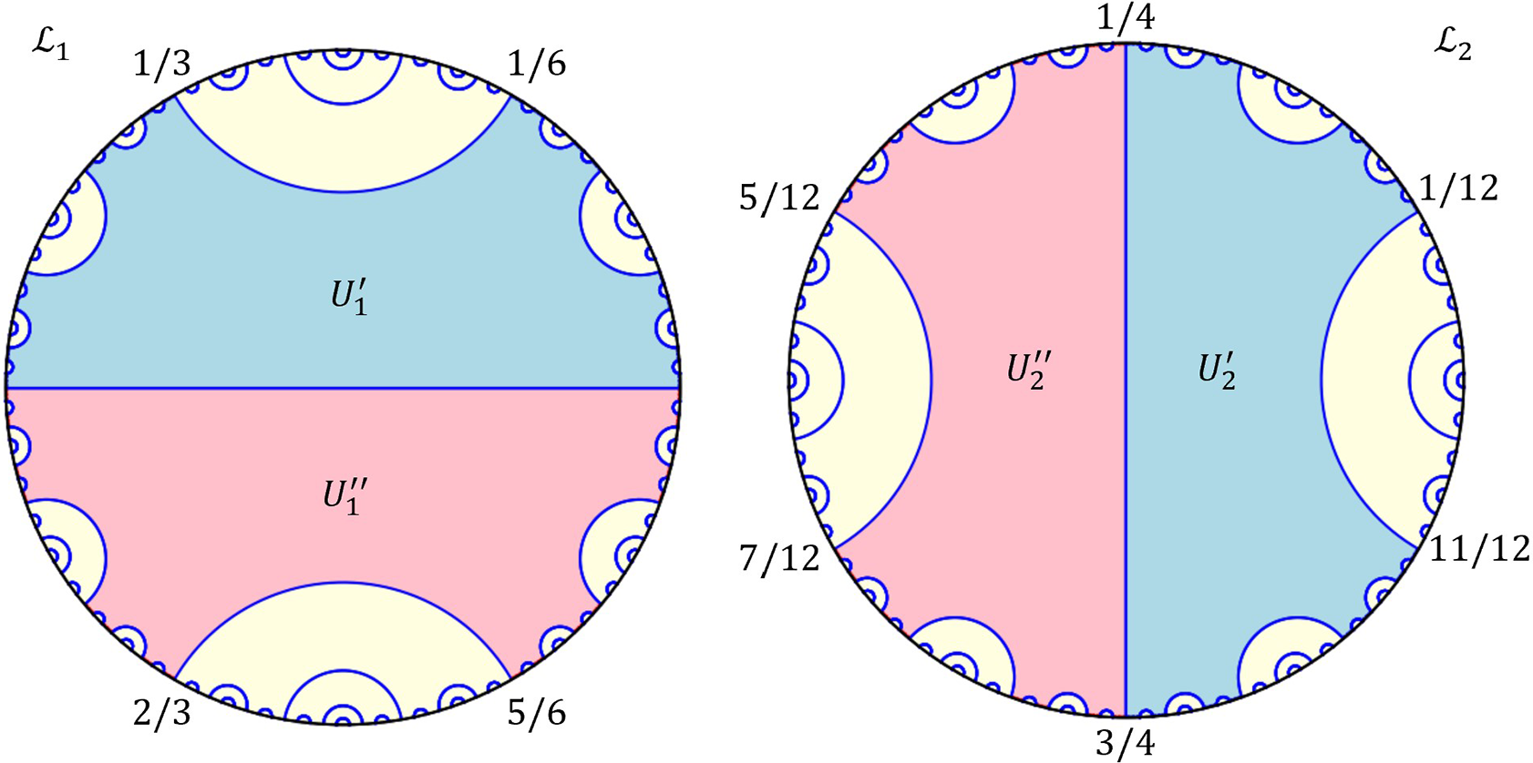
Lemma 3.20. [Reference Blokh, Oversteegen, Selinger, Timorin and VejandlaBOSTV1, Lemma 5.8]
There are only two symmetric cubic laminations $\mathcal {L}_1$
,
$\mathcal {L}_1$
, $\mathcal {L}_2$
with comajors of length
$\mathcal {L}_2$
with comajors of length $\frac 16$
, namely as follows.
$\frac 16$
, namely as follows. $(1)$
The lamination
$(1)$
The lamination $\mathcal {L}_1$
has comajors
$\mathcal {L}_1$
has comajors $\overline {\tfrac 16 \frac 13}$
,
$\overline {\tfrac 16 \frac 13}$
, $\overline {\tfrac 23 \frac 56}$
and invariant critical Fatou gaps
$\overline {\tfrac 23 \frac 56}$
and invariant critical Fatou gaps $U^{\prime }_1$
,
$U^{\prime }_1$
, $U^{\prime \prime }_1$
, where
$U^{\prime \prime }_1$
, where $U^{\prime }_1\cap \mathbb {S}$
consists of all
$U^{\prime }_1\cap \mathbb {S}$
consists of all $\gamma \in \mathbb {S}$
such that
$\gamma \in \mathbb {S}$
such that $\sigma _3^n(\gamma )\in [0, \frac 12]$
(for all n), and
$\sigma _3^n(\gamma )\in [0, \frac 12]$
(for all n), and $U^{\prime }_1\cap \mathbb {S}$
consists of all
$U^{\prime }_1\cap \mathbb {S}$
consists of all $\gamma \in \mathbb {S}$
such that
$\gamma \in \mathbb {S}$
such that $\sigma _3^n(\gamma )\in [\frac 12, 0]$
. The gaps
$\sigma _3^n(\gamma )\in [\frac 12, 0]$
. The gaps $U_1^{\prime }$
,
$U_1^{\prime }$
, $U_1^{\prime \prime }$
share the edge
$U_1^{\prime \prime }$
share the edge $\overline {0 \frac 12}$
; their other edges are the appropriate iterated pullbacks of
$\overline {0 \frac 12}$
; their other edges are the appropriate iterated pullbacks of $\overline {0\frac 12}$
that never separate
$\overline {0\frac 12}$
that never separate $\overline {\tfrac 16 \frac 13}$
,
$\overline {\tfrac 16 \frac 13}$
, $\overline {\tfrac 23 \frac 56}$
, and
$\overline {\tfrac 23 \frac 56}$
, and $\overline {0\frac 12}$
.
$\overline {0\frac 12}$
. $(2)$
The lamination
$(2)$
The lamination $\mathcal {L}_2$
has comajors
$\mathcal {L}_2$
has comajors $\overline {\tfrac {11}{12}\tfrac {1}{12}}$
,
$\overline {\tfrac {11}{12}\tfrac {1}{12}}$
, $\overline {\tfrac {5}{12} \tfrac {7}{12}}$
and critical Fatou gaps
$\overline {\tfrac {5}{12} \tfrac {7}{12}}$
and critical Fatou gaps $U^{\prime }_2$
,
$U^{\prime }_2$
, $U^{\prime \prime }_2$
that form a 2-cycle, where the set
$U^{\prime \prime }_2$
that form a 2-cycle, where the set $(U_2'\cup U_2^{\prime \prime })\cap \mathbb {S}$
consists of all
$(U_2'\cup U_2^{\prime \prime })\cap \mathbb {S}$
consists of all $\gamma \in \mathbb {S}$
such that
$\gamma \in \mathbb {S}$
such that $\sigma _3^n(\gamma )\in [\tfrac 1{12}, \tfrac 5{12}]\cup [\tfrac 7{12}, \tfrac {11}{12}]$
. The gaps
$\sigma _3^n(\gamma )\in [\tfrac 1{12}, \tfrac 5{12}]\cup [\tfrac 7{12}, \tfrac {11}{12}]$
. The gaps $U_2^{\prime }$
,
$U_2^{\prime }$
, $U_2^{\prime \prime }$
share the edge
$U_2^{\prime \prime }$
share the edge $\overline {\tfrac 14 \tfrac 34}$
; their other edges are the appropriate iterated pullbacks of
$\overline {\tfrac 14 \tfrac 34}$
; their other edges are the appropriate iterated pullbacks of $\overline {\tfrac 14 \tfrac 34}$
that never separate
$\overline {\tfrac 14 \tfrac 34}$
that never separate $\overline {\tfrac {11}{12} \tfrac {1}{12}}$
,
$\overline {\tfrac {11}{12} \tfrac {1}{12}}$
, $\overline {\tfrac {5}{12} \tfrac {7}{12}}$
, and
$\overline {\tfrac {5}{12} \tfrac {7}{12}}$
, and $\overline {\tfrac 14 \tfrac 34}$
.
$\overline {\tfrac 14 \tfrac 34}$
.
Though the laminations from Lemma 3.20 are not the pullback laminations described below, knowing them allows us to consider only legal pairs with comajors of length less than $\frac 16$
and streamline the proofs.
$\frac 16$
and streamline the proofs.
The construction below repeats that from [Reference Blokh, Oversteegen, Selinger, Timorin and VejandlaBOSTV1]; we add it here for the sake of completeness and convenience of the reader.
3.1 Construction of a symmetric pullback lamination
$\mathcal {L}(c)$
for a legal pair
$\{c, -c\}$


3.1.1 Degenerate case
For $c\in \mathbb {S}$
, let
$c\in \mathbb {S}$
, let $\pm \ell =\pm M_c$
(call
$\pm \ell =\pm M_c$
(call $\ell $
,
$\ell $
, $-\ell $
, and their pullbacks ‘leaves’ even though we apply this term to existing laminations and we are only constructing one). Consider two cases.
$-\ell $
, and their pullbacks ‘leaves’ even though we apply this term to existing laminations and we are only constructing one). Consider two cases.
(a) If $\ell $
and
$\ell $
and $-\ell $
do not have periodic endpoints, then the family of all iterated pullbacks of
$-\ell $
do not have periodic endpoints, then the family of all iterated pullbacks of $\ell , -\ell $
generated by
$\ell , -\ell $
generated by $\ell , -\ell $
is denoted by
$\ell , -\ell $
is denoted by $\mathcal {C}_c$
(see Figure 5).
$\mathcal {C}_c$
(see Figure 5).
The pullback construction in the degenerate non-periodic case. The two critical leaves are shown in boldface, their first pullbacks are in normal, second pullbacks are dashed, and third pullbacks are dotted.
(b) Suppose that $\ell $
and
$\ell $
and $-\ell $
have periodic endpoints p and
$-\ell $
have periodic endpoints p and $-p$
. Then, there are two similar cases. First, the orbits of p and
$-p$
. Then, there are two similar cases. First, the orbits of p and $-p$
may be distinct (and hence disjoint). Then, iterated pullbacks of
$-p$
may be distinct (and hence disjoint). Then, iterated pullbacks of $\ell $
generated by
$\ell $
generated by $\ell $
,
$\ell $
, $-\ell $
are well defined (unique) until the nth step (n equals the period of p and the period of
$-\ell $
are well defined (unique) until the nth step (n equals the period of p and the period of $-p$
), when there are two iterated pullbacks of
$-p$
), when there are two iterated pullbacks of $\ell $
that have a common endpoint x and share other endpoints with
$\ell $
that have a common endpoint x and share other endpoints with $\ell $
. Two other iterated pullbacks of
$\ell $
. Two other iterated pullbacks of $\ell $
have a common endpoint
$\ell $
have a common endpoint $y\ne 0$
and share other endpoints with
$y\ne 0$
and share other endpoints with $\ell $
. These four iterated pullbacks of
$\ell $
. These four iterated pullbacks of $\ell $
form a collapsing quadrilateral Q with diagonal
$\ell $
form a collapsing quadrilateral Q with diagonal $\ell $
; moreover,
$\ell $
; moreover, $\sigma _3(x)=\sigma _3(y)$
and
$\sigma _3(x)=\sigma _3(y)$
and $\sigma _3^n(x)=\sigma _3^n(y)=z$
is the non-periodic endpoint of
$\sigma _3^n(x)=\sigma _3^n(y)=z$
is the non-periodic endpoint of $\ell $
. Evidently,
$\ell $
. Evidently, $\sigma _3(Q)=\overline {\sigma _3(p)\sigma _3(x)}$
is the
$\sigma _3(Q)=\overline {\sigma _3(p)\sigma _3(x)}$
is the $(n-1)$
st iterated pullback of
$(n-1)$
st iterated pullback of $\ell $
. Then, in the pullback lamination
$\ell $
. Then, in the pullback lamination $\mathcal {L}(c)$
that we are defining, we postulate the choice of only the short pullbacks among the above listed iterated pullbacks of
$\mathcal {L}(c)$
that we are defining, we postulate the choice of only the short pullbacks among the above listed iterated pullbacks of $\ell $
(see Figure 3(b)). So, only two short edges of Q are included in the set of pullbacks
$\ell $
(see Figure 3(b)). So, only two short edges of Q are included in the set of pullbacks $\mathcal {C}_c$
. A similar situation holds for
$\mathcal {C}_c$
. A similar situation holds for $-\ell $
and its iterated pullbacks.
$-\ell $
and its iterated pullbacks.
In general, the choice of pullbacks of the already constructed leaf $\hat {\ell }$
is ambiguous only if
$\hat {\ell }$
is ambiguous only if $\hat {\ell }$
has an endpoint
$\hat {\ell }$
has an endpoint $\sigma _3(\pm \ell )$
. In this case, we always choose short pullbacks of
$\sigma _3(\pm \ell )$
. In this case, we always choose short pullbacks of $\hat {\ell }$
. Evidently, this defines a set
$\hat {\ell }$
. Evidently, this defines a set $\mathcal {C}_c$
of chords in a unique way.
$\mathcal {C}_c$
of chords in a unique way.
We claim that $\mathcal {C}_c$
is an invariant prelamination. To show that
$\mathcal {C}_c$
is an invariant prelamination. To show that $\mathcal {C}_c$
is a prelamination, we need to show that its leaves do not cross. Suppose otherwise and choose the minimal n such that
$\mathcal {C}_c$
is a prelamination, we need to show that its leaves do not cross. Suppose otherwise and choose the minimal n such that $\hat {\ell }$
and
$\hat {\ell }$
and $\tilde {\ell }$
are pullbacks of
$\tilde {\ell }$
are pullbacks of $\ell $
or
$\ell $
or $-\ell $
under at most the nth iterate of
$-\ell $
under at most the nth iterate of $\sigma _3$
that cross. By construction,
$\sigma _3$
that cross. By construction, $\hat {\ell }, \tilde {\ell }$
are not critical. Hence, their images
$\hat {\ell }, \tilde {\ell }$
are not critical. Hence, their images $\sigma _3(\hat {\ell })$
,
$\sigma _3(\hat {\ell })$
, $\sigma _3(\tilde {\ell })$
are not degenerate and do not cross. It is only possible if
$\sigma _3(\tilde {\ell })$
are not degenerate and do not cross. It is only possible if $\hat {\ell }, \tilde {\ell }$
come out of the endpoints of a critical leaf of
$\hat {\ell }, \tilde {\ell }$
come out of the endpoints of a critical leaf of $\mathcal {L}$
. We may assume that
$\mathcal {L}$
. We may assume that $\|\hat {\ell }\|\ge \frac 16$
(if
$\|\hat {\ell }\|\ge \frac 16$
(if $\hat {\ell }$
and
$\hat {\ell }$
and $\tilde {\ell }$
are shorter than
$\tilde {\ell }$
are shorter than $\frac 16$
, then they cannot cross). However, by construction, this is impossible. Hence,
$\frac 16$
, then they cannot cross). However, by construction, this is impossible. Hence, $\mathcal {C}_c$
is a prelamination. The claim that
$\mathcal {C}_c$
is a prelamination. The claim that $\mathcal {C}_c$
is invariant is straightforward; its verification is left to the reader. By Theorem 2.14, the closure of
$\mathcal {C}_c$
is invariant is straightforward; its verification is left to the reader. By Theorem 2.14, the closure of $\mathcal {C}_c$
is an invariant lamination denoted
$\mathcal {C}_c$
is an invariant lamination denoted $\mathcal {L}(c)$
. Moreover, by construction,
$\mathcal {L}(c)$
. Moreover, by construction, $\mathcal {C}_c$
is symmetric (this can be easily proven using induction on the number of steps in the process of pulling back
$\mathcal {C}_c$
is symmetric (this can be easily proven using induction on the number of steps in the process of pulling back $\ell $
and
$\ell $
and $-\ell $
). Hence,
$-\ell $
). Hence, $\mathcal {L}(c)$
is a symmetric invariant lamination. See Figure 7(a), for an illustration of
$\mathcal {L}(c)$
is a symmetric invariant lamination. See Figure 7(a), for an illustration of $\mathcal {L}(c)$
.
$\mathcal {L}(c)$
.
3.1.2 Non-degenerate case
As in the degenerate case, we will talk about pullback leaves even though we are still constructing a lamination. By Lemma 3.20, we may assume that $|c|<\frac 16$
. Set
$|c|<\frac 16$
. Set $\pm M=\pm M_c, \pm Q=\pm Q_c$
. If d is an iterated forward image of c or
$\pm M=\pm M_c, \pm Q=\pm Q_c$
. If d is an iterated forward image of c or $-c$
, then, by Definition 3.18(b), it cannot intersect the interior Q or
$-c$
, then, by Definition 3.18(b), it cannot intersect the interior Q or $-Q$
. Consider the set of leaves
$-Q$
. Consider the set of leaves $\mathcal {D}$
formed by the edges of
$\mathcal {D}$
formed by the edges of $\pm Q$
and
$\pm Q$
and $\bigcup _{m=0}^{\infty }\{\sigma _3^{m}(c),\sigma _3^{m}(-c)\}$
. It follows that leaves of
$\bigcup _{m=0}^{\infty }\{\sigma _3^{m}(c),\sigma _3^{m}(-c)\}$
. It follows that leaves of $\mathcal {D}$
do not cross among themselves. The idea is to construct pullbacks of leaves of
$\mathcal {D}$
do not cross among themselves. The idea is to construct pullbacks of leaves of $\mathcal {D}$
in a step-by-step fashion and show that this results in an invariant prelamination
$\mathcal {D}$
in a step-by-step fashion and show that this results in an invariant prelamination $\mathcal {C}_c$
as in the degenerate case.
$\mathcal {C}_c$
as in the degenerate case.
More precisely, we proceed by induction. Set $\mathcal {D}=\mathcal {C}_c^0$
. Construct sets of leaves
$\mathcal {D}=\mathcal {C}_c^0$
. Construct sets of leaves $\mathcal {C}_c^{n+1}$
by collecting pullbacks of leaves of
$\mathcal {C}_c^{n+1}$
by collecting pullbacks of leaves of $\mathcal {C}_c^{n}$
generated by Q and
$\mathcal {C}_c^{n}$
generated by Q and $-Q$
(the step of induction is based upon Definitions 3.18 and 3.19). The claim is that except for the property (D2)(1) from Definition 2.6 (a part of what it means for a lamination to be backward invariant), the set
$-Q$
(the step of induction is based upon Definitions 3.18 and 3.19). The claim is that except for the property (D2)(1) from Definition 2.6 (a part of what it means for a lamination to be backward invariant), the set $\mathcal {C}_c^n$
has all the properties of invariant laminations listed in Definition 2.6. Let us verify this property for
$\mathcal {C}_c^n$
has all the properties of invariant laminations listed in Definition 2.6. Let us verify this property for $\mathcal {C}_c^1$
. Let
$\mathcal {C}_c^1$
. Let $\ell \in \mathcal {C}_c^1$
. Then,
$\ell \in \mathcal {C}_c^1$
. Then, $\sigma _3(\ell )\in \mathcal {D}$
, so property (D1) from Definition 2.6 is satisfied. Property (D2)(2) is, evidently, satisfied for edges of Q and
$\sigma _3(\ell )\in \mathcal {D}$
, so property (D1) from Definition 2.6 is satisfied. Property (D2)(2) is, evidently, satisfied for edges of Q and $-Q$
. If
$-Q$
. If $\ell $
is not an edge of
$\ell $
is not an edge of $\pm Q$
, then, since leaves
$\pm Q$
, then, since leaves $\pm \sigma _3(Q)=\sigma _3(\pm c)$
do not cross
$\pm \sigma _3(Q)=\sigma _3(\pm c)$
do not cross $\sigma (\ell )$
, and since on the closure of each component of
$\sigma (\ell )$
, and since on the closure of each component of $\mathbb {S}\setminus [Q\cup -Q]$
the map is one-to-one, then
$\mathbb {S}\setminus [Q\cup -Q]$
the map is one-to-one, then $\ell $
will have two sibling leaves in
$\ell $
will have two sibling leaves in $\mathcal {C}_c^1$
as desired. Literally the same argument works for
$\mathcal {C}_c^1$
as desired. Literally the same argument works for $\ell \in \mathcal {C}_c^{n+1}$
and proves that each set
$\ell \in \mathcal {C}_c^{n+1}$
and proves that each set $\mathcal {C}_c^{n+1}$
has properties (D1) and (D2)(2) from Definition 2.6. This implies that
$\mathcal {C}_c^{n+1}$
has properties (D1) and (D2)(2) from Definition 2.6. This implies that $\bigcup _{i\ge 0} \mathcal {C}_c^i=\mathcal {C}_c$
has all properties from Definition 2.6 and is, therefore, an invariant prelamination. By Theorem 2.14, its closure
$\bigcup _{i\ge 0} \mathcal {C}_c^i=\mathcal {C}_c$
has all properties from Definition 2.6 and is, therefore, an invariant prelamination. By Theorem 2.14, its closure $\mathcal {L}(c)$
is an invariant lamination.
$\mathcal {L}(c)$
is an invariant lamination.
The lamination $\mathcal {L}(c)$
is called the pullback lamination (of c); we often use c as the argument, instead of the less discriminatory
$\mathcal {L}(c)$
is called the pullback lamination (of c); we often use c as the argument, instead of the less discriminatory $\{c, -c\}$
.
$\{c, -c\}$
.
Lemma 3.21. [Reference Blokh, Oversteegen, Selinger, Timorin and VejandlaBOSTV1, Lemma 5.9]
A legal pair $\{c,-c\}$
is the comajor pair of the lamination
$\{c,-c\}$
is the comajor pair of the lamination $\mathcal {L}(c)$
. A symmetric pair
$\mathcal {L}(c)$
. A symmetric pair $\{c, -c\}$
is a comajor pair if and only if it is legal.
$\{c, -c\}$
is a comajor pair if and only if it is legal.
Theorem 3.22 contains the main results of [Reference Blokh, Oversteegen, Selinger, Timorin and VejandlaBOSTV1]. Co-periodic comajors are defined as preperiodic comajors of preperiod 1. The name is due to the fact that a co-periodic comajor is a sibling of a periodic major.
Theorem 3.22. The set of all comajors of cubic symmetric laminations is a q-lamination. Co-periodic comajors are disjoint from all other comajors.
Based on this theorem, we define the main object of our interest.
Definition 3.23. All comajors of cubic symmetric laminations form a lamination $C_sCL$
called the cubic symmetric comajor lamination.
$C_sCL$
called the cubic symmetric comajor lamination.
The following useful notation is justified by Theorem 3.22.
Definition 3.24. For a non-diameter chord $n=\overline {ab}$
, the smaller of the two arcs into which n divides
$n=\overline {ab}$
, the smaller of the two arcs into which n divides $\mathbb {S}$
is denoted by
$\mathbb {S}$
is denoted by $H(n)$
. Denote the closed subset of
$H(n)$
. Denote the closed subset of $\overline {\mathbb {D}}$
bounded by n and
$\overline {\mathbb {D}}$
bounded by n and $H(n)$
by
$H(n)$
by $R(n)$
. Given two comajors m and n, write
$R(n)$
. Given two comajors m and n, write $m\prec n$
if
$m\prec n$
if $m\subset R(n)$
, and say that m is under n.
$m\subset R(n)$
, and say that m is under n.
Lemma 3.25. [Reference Blokh, Oversteegen, Selinger, Timorin and VejandlaBOSTV1, Lemma 5.14]
Let $\{c,-c\}$
and
$\{c,-c\}$
and $\{d,-d\}$
be legal pairs, where c is degenerate and
$\{d,-d\}$
be legal pairs, where c is degenerate and $c\prec d$
. Suppose that c is not an endpoint of d, or
$c\prec d$
. Suppose that c is not an endpoint of d, or $\sigma _3(c)$
is not periodic. Then,
$\sigma _3(c)$
is not periodic. Then, $d\in \mathcal {L}(c)$
. In addition, the following holds.
$d\in \mathcal {L}(c)$
. In addition, the following holds.
-
(1) Majors D,
$D'$
of
$\mathcal {L}(d)$
are leaves of
$\mathcal {L}(c)$
unless
$\mathcal {L}(c)$
has two finite gaps
$G, G'$
that contain
$D, D'$
as their diagonals, share a critical leaf M of
$\mathcal {L}(c)$
as a common edge, and are such that
$\sigma _3(G)=\sigma _3(G')$
is a preperiodic gap. -
(2) If majors of
$\mathcal {L}(d)$
are leaves of
$\mathcal {L}(c)$
and
$\ell \in \mathcal {L}(d)$
is a leaf that never maps to a short side of a collapsing quadrilateral of
$\mathcal {L}(d)$
, then
$\ell \in \mathcal {L}(c)$
.


4 Combinatorial analog of the Fatou conjecture on density of hyperbolicity
We begin by stating a few results that will be used in what follows.
Definition 4.1. If a symmetric lamination $\mathcal {L}$
has a periodic Fatou gap of degree greater than
$\mathcal {L}$
has a periodic Fatou gap of degree greater than $1$
(that is, if it has properties listed in Lemma 4.10), then
$1$
(that is, if it has properties listed in Lemma 4.10), then $\mathcal {L}$
is called hyperbolic.
$\mathcal {L}$
is called hyperbolic.
We need a result of [Reference Blokh, Mimbs, Oversteegen and ValkenburgBMOV13]. Recall that, as in Definition 2.5, a lamination $\mathcal {L}$
generates an equivalence relation
$\mathcal {L}$
generates an equivalence relation $\sim _{\mathcal {L}}$
on
$\sim _{\mathcal {L}}$
on $\mathbb {S}$
by declaring that
$\mathbb {S}$
by declaring that $a\sim _{\mathcal {L}} b$
if and only if a finite concatenation of leaves of
$a\sim _{\mathcal {L}} b$
if and only if a finite concatenation of leaves of $\mathcal {L}$
connects points
$\mathcal {L}$
connects points $a\in \mathbb {S}$
and
$a\in \mathbb {S}$
and $b\in \mathbb {S}$
.
$b\in \mathbb {S}$
.
Definition 4.2. (Proper lamination, [Reference Blokh, Mimbs, Oversteegen and ValkenburgBMOV13, Definition 4.1])
Two leaves with a common endpoint v and the same image which is a leaf (and not a point) are said to form a critical wedge (the point v then is said to be its vertex). A lamination $\mathcal {L}$
is proper if it contains no critical leaf with periodic endpoint and no critical wedge with periodic vertex.
$\mathcal {L}$
is proper if it contains no critical leaf with periodic endpoint and no critical wedge with periodic vertex.
Proper laminations generate laminational equivalence relations.
Theorem 4.3. [Reference Blokh, Mimbs, Oversteegen and ValkenburgBMOV13, Theorem 4.9]
Let $\mathcal {L}$
be a proper invariant lamination. Then,
$\mathcal {L}$
be a proper invariant lamination. Then, $\sim _{\mathcal {L}}$
is an invariant laminational equivalence relation.
$\sim _{\mathcal {L}}$
is an invariant laminational equivalence relation.
We also need a nice result due to Kiwi [Reference KiwiKiw02].
Theorem 4.4. [Reference KiwiKiw02]
Let $\mathcal {L}$
be a
$\mathcal {L}$
be a $\sigma _d$
-invariant lamination. Then, any infinite gap of
$\sigma _d$
-invariant lamination. Then, any infinite gap of $\mathcal {L}$
is (pre)periodic. For any finite periodic gap G of
$\mathcal {L}$
is (pre)periodic. For any finite periodic gap G of $\mathcal {L}$
, its vertices belong to at most
$\mathcal {L}$
, its vertices belong to at most $d-1$
distinct cycles except when G is a fixed return d-gon. In particular, a cubic lamination cannot have a fixed return n-gon for
$d-1$
distinct cycles except when G is a fixed return d-gon. In particular, a cubic lamination cannot have a fixed return n-gon for $n>3$
. Moreover, if all images of a k-gon G with
$n>3$
. Moreover, if all images of a k-gon G with $k>d$
have at least
$k>d$
have at least $d+1$
vertices, then G is preperiodic.
$d+1$
vertices, then G is preperiodic.
Finally, here are several important claims from [Reference Blokh, Oversteegen, Selinger, Timorin and VejandlaBOSTV1].
Corollary 4.5. [Reference Blokh, Oversteegen, Selinger, Timorin and VejandlaBOSTV1, Corollary 4.8]
If E is a preperiodic polygon of a symmetric lamination such that E is not precritical, then no diagonal of E can be a leaf of a symmetric lamination.
Lemma 4.6. [Reference Blokh, Oversteegen, Selinger, Timorin and VejandlaBOSTV1, Lemma 6.2]
Let $c\in C_sCL$
be a non-degenerate comajor. If
$c\in C_sCL$
be a non-degenerate comajor. If ${\ell \in \mathcal {L}(c),}$ $\ell \prec c$
, and
$\ell \prec c$
, and $\|\ell \|>{\|c\|}/{3}$
, then
$\|\ell \|>{\|c\|}/{3}$
, then $\ell \in C_sCL$
. In particular, if
$\ell \in C_sCL$
. In particular, if $c_i\in \mathcal {L}(c)$
,
$c_i\in \mathcal {L}(c)$
, $c_i\prec c$
, and
$c_i\prec c$
, and $c_i \rightarrow c$
, then
$c_i \rightarrow c$
, then $c_n\in C_sCL$
for sufficiently large n.
$c_n\in C_sCL$
for sufficiently large n.
Lemma 4.7. [Reference Blokh, Oversteegen, Selinger, Timorin and VejandlaBOSTV1, Lemma 6.6]
Let $c\in C_sCL$
be a non-degenerate comajor such that
$c\in C_sCL$
be a non-degenerate comajor such that $\sigma _3(c)$
is not periodic. If there exists a sequence of leaves
$\sigma _3(c)$
is not periodic. If there exists a sequence of leaves $c_i\in \mathcal {L}(c)$
with
$c_i\in \mathcal {L}(c)$
with $c\prec c_i$
and
$c\prec c_i$
and $c_i\rightarrow c,$
then c is the limit of co-periodic comajors
$c_i\rightarrow c,$
then c is the limit of co-periodic comajors $\hat {c}_j \in \mathcal {L}(c)$
with
$\hat {c}_j \in \mathcal {L}(c)$
with $c\prec \hat {c}_j$
for all j.
$c\prec \hat {c}_j$
for all j.
Corollary 4.8. [Reference Blokh, Oversteegen, Selinger, Timorin and VejandlaBOSTV1, Corollary 6.7]
Every not eventually periodic comajor c is a two-sided limit leaf in the cubic symmetric comajor lamination $C_sCL$
.
$C_sCL$
.
Lemma 4.9. [Reference Blokh, Oversteegen, Selinger, Timorin and VejandlaBOSTV1, Lemma 6.8]
A co-major which is non-degenerate and preperiodic of preperiod at least $2$
is a two-sided limit leaf of
$2$
is a two-sided limit leaf of $C_sCL$
or an edge of a finite gap H of
$C_sCL$
or an edge of a finite gap H of $C_sCL$
all of whose edges are limits of comajors of
$C_sCL$
all of whose edges are limits of comajors of $C_sCL$
disjoint from H.
$C_sCL$
disjoint from H.
Let us now describe laminations related to co-periodic comajors.
Lemma 4.10. Let $\mathcal {L}$
be a symmetric lamination with a periodic Fatou gap of degree greater than
$\mathcal {L}$
be a symmetric lamination with a periodic Fatou gap of degree greater than $1$
. Then,
$1$
. Then, $\mathcal {L}$
has two critical Fatou gaps of degree greater than
$\mathcal {L}$
has two critical Fatou gaps of degree greater than $1$
. Moreover,
$1$
. Moreover, $\mathcal {L}$
is a q-lamination.
$\mathcal {L}$
is a q-lamination.
Proof. Because of the symmetry, a hyperbolic symmetric lamination $\mathcal {L}$
has two critical Fatou gaps of degree greater than
$\mathcal {L}$
has two critical Fatou gaps of degree greater than $1$
. These gaps either belong to the same cycle of Fatou gaps, or belong to two distinct cycles of Fatou gaps. Moreover, by Theorem 4.3, the equivalence
$1$
. These gaps either belong to the same cycle of Fatou gaps, or belong to two distinct cycles of Fatou gaps. Moreover, by Theorem 4.3, the equivalence $\sim _{\mathcal {L}}$
is laminational. We claim that
$\sim _{\mathcal {L}}$
is laminational. We claim that $\mathcal {L}$
coincides with the q-lamination
$\mathcal {L}$
coincides with the q-lamination $\widehat {\mathcal {L}}$
generated by
$\widehat {\mathcal {L}}$
generated by $\sim _{\mathcal {L}}$
. We need to show that any leaf of
$\sim _{\mathcal {L}}$
. We need to show that any leaf of $\mathcal {L}$
is a leaf of
$\mathcal {L}$
is a leaf of $\widehat {\mathcal {L}}$
.
$\widehat {\mathcal {L}}$
.
In general, edges of a Fatou gap U may form a finite concatenation, in which case, U is not a gap of the corresponding q-lamination (by definition, in the q-lamination, we add one more leaf to the concatenation to make it into a finite gap; this extra leaf will be an edge of a new, smaller Fatou gap of the q-lamination). However, this cannot happen in our case: if it did, it would yield a symmetric q-lamination with fixed return finite gaps contradicting Lemma 3.10. Hence, the Fatou gaps of $\mathcal {L}$
are gaps of
$\mathcal {L}$
are gaps of $\widehat {\mathcal {L}}$
. Otherwise, if
$\widehat {\mathcal {L}}$
. Otherwise, if $\ell \in \mathcal {L}$
is not a leaf of
$\ell \in \mathcal {L}$
is not a leaf of $\widehat {\mathcal {L}}$
, then
$\widehat {\mathcal {L}}$
, then $\ell $
must be a diagonal of a finite gap G of
$\ell $
must be a diagonal of a finite gap G of $\widehat {\mathcal {L}}$
. However, by Corollary 4.5, this is impossible. Hence,
$\widehat {\mathcal {L}}$
. However, by Corollary 4.5, this is impossible. Hence, $\mathcal {L}=\widehat {\mathcal {L}}$
is a q-lamination as desired.
$\mathcal {L}=\widehat {\mathcal {L}}$
is a q-lamination as desired.
Hyperbolic laminations are constructed in Theorem 4.11.
Theorem 4.11. A preperiodic point $q\in \mathbb {S}$
of preperiod
$q\in \mathbb {S}$
of preperiod $1$
and period k is an endpoint of a non-degenerate co-periodic comajor c of period k of a cubic symmetric lamination. Take the short edges of
$1$
and period k is an endpoint of a non-degenerate co-periodic comajor c of period k of a cubic symmetric lamination. Take the short edges of $\pm Q_c$
, and remove their backward orbits from
$\pm Q_c$
, and remove their backward orbits from $\mathcal {L}(c)$
. Then, the resulting lamination
$\mathcal {L}(c)$
. Then, the resulting lamination $\widehat {\mathcal {L}}(c)$
is a hyperbolic q-lamination with comajor pair
$\widehat {\mathcal {L}}(c)$
is a hyperbolic q-lamination with comajor pair $\{c, -c\}$
.
$\{c, -c\}$
.
Proof. Let $\ell =\overline {x_0p}$
be the critical leaf with
$\ell =\overline {x_0p}$
be the critical leaf with $\sigma _3(\ell )=\sigma _3(q)$
and a k-periodic endpoint p. Consider the pullback lamination
$\sigma _3(\ell )=\sigma _3(q)$
and a k-periodic endpoint p. Consider the pullback lamination $\mathcal {L}(q)$
. Let G be the central symmetric gap or leaf of
$\mathcal {L}(q)$
. Let G be the central symmetric gap or leaf of $\mathcal {L}(q)$
located between
$\mathcal {L}(q)$
located between $\ell $
and
$\ell $
and $-\ell $
. Then, G contains the origin and has leaves
$-\ell $
. Then, G contains the origin and has leaves $\pm M$
closest to criticality. Let
$\pm M$
closest to criticality. Let $M'$
and d be the medium and short siblings of M. Clearly, the short siblings
$M'$
and d be the medium and short siblings of M. Clearly, the short siblings $\pm d$
of leaves
$\pm d$
of leaves $\pm M$
form a legal pair. Hence, if
$\pm M$
form a legal pair. Hence, if $\ell $
shares an endpoint with M, then, by Lemma 3.21, we can set
$\ell $
shares an endpoint with M, then, by Lemma 3.21, we can set $c=d$
. Assume now that leaves
$c=d$
. Assume now that leaves $\pm \ell $
are disjoint from
$\pm \ell $
are disjoint from $\pm M$
.
$\pm M$
.
If the orbits of p and $-p$
are disjoint, let
$-p$
are disjoint, let $n=k$
. Otherwise,
$n=k$
. Otherwise, $k=2n$
for some n, while
$k=2n$
for some n, while $\sigma _3^n(p)=-p$
and
$\sigma _3^n(p)=-p$
and $\sigma _3^n(-p)=p$
. We will assume in the rest of the proof that
$\sigma _3^n(-p)=p$
. We will assume in the rest of the proof that $k=n$
; the case
$k=n$
; the case $k=2n$
is similar. Observe that
$k=2n$
is similar. Observe that $\mathcal {L}(q)$
contains the critical leaf
$\mathcal {L}(q)$
contains the critical leaf $\ell =\overline {x_0p}$
with periodic endpoint p, which in fact implies that
$\ell =\overline {x_0p}$
with periodic endpoint p, which in fact implies that $\mathcal {L}(q)$
contains caterpillar gaps (see Figure 6). Indeed, consider the strip S between M and
$\mathcal {L}(q)$
contains caterpillar gaps (see Figure 6). Indeed, consider the strip S between M and $M'$
. Let
$M'$
. Let $s=\overline {x_0x_1}$
be the short pullback of
$s=\overline {x_0x_1}$
be the short pullback of $\ell $
under
$\ell $
under $\sigma _3^k$
, which is included in
$\sigma _3^k$
, which is included in $\mathcal {L}(q)$
by construction; then
$\mathcal {L}(q)$
by construction; then $\sigma _3^k(s)=\overline {x_0p}$
. Hence, there is another leaf
$\sigma _3^k(s)=\overline {x_0p}$
. Hence, there is another leaf $\overline {x_1x_2}$
such that
$\overline {x_1x_2}$
such that $\sigma _3^k(\overline {x_1x_2})=\overline {x_0x_1}$
. The leaf
$\sigma _3^k(\overline {x_1x_2})=\overline {x_0x_1}$
. The leaf $\overline {x_1x_2}$
is short as if
$\overline {x_1x_2}$
is short as if $\overline {x_1x_2}$
is long/medium, then its kth image s is short and non-disjoint from the interior of its short strips, contradicting Lemma 3.8. Repeating this, we get a concatenation A of pullbacks of
$\overline {x_1x_2}$
is long/medium, then its kth image s is short and non-disjoint from the interior of its short strips, contradicting Lemma 3.8. Repeating this, we get a concatenation A of pullbacks of $\ell $
under powers of
$\ell $
under powers of $\sigma _3^k$
; A consists of short leaves of
$\sigma _3^k$
; A consists of short leaves of $\mathcal {L}(q)$
, begins with
$\mathcal {L}(q)$
, begins with $\ell \cup \overline {x_0x_1}\cup \overline {x_1x_2}$
, converges to a point
$\ell \cup \overline {x_0x_1}\cup \overline {x_1x_2}$
, converges to a point $t\in \mathbb {S}$
of period k, and points
$t\in \mathbb {S}$
of period k, and points $x_0, x_1, \ldots $
belong to the short circular arc I that bounds S and does not contain p. Since t and p belong to distinct circle arcs on the boundary of S, then
$x_0, x_1, \ldots $
belong to the short circular arc I that bounds S and does not contain p. Since t and p belong to distinct circle arcs on the boundary of S, then $t\ne p$
.
$t\ne p$
.
Illustration of the proof of Theorem 4.11.
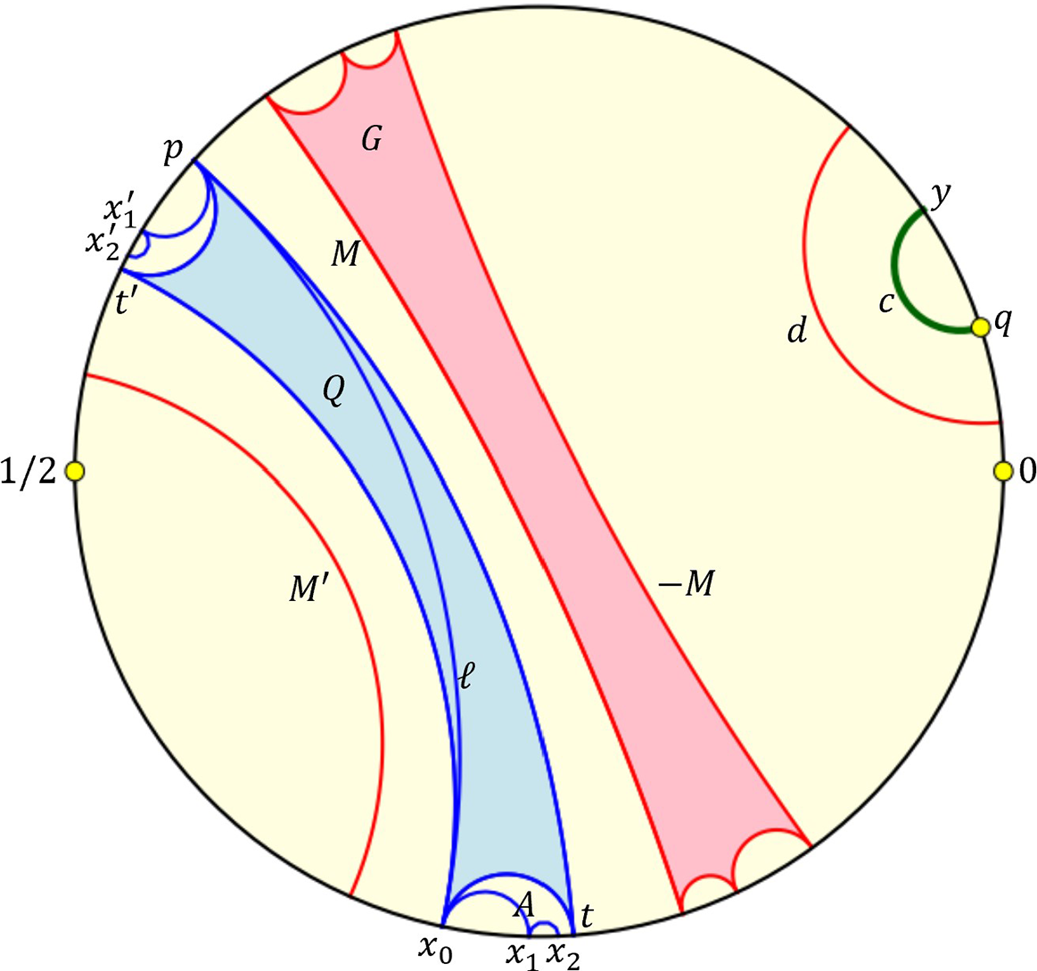
Clearly, an infinite periodic gap U of $\mathcal {L}(q)$
contains A in its boundary, and there is a gap
$\mathcal {L}(q)$
contains A in its boundary, and there is a gap $U'$
with the same image as U that shares an edge
$U'$
with the same image as U that shares an edge $\ell $
with U. Consider the chord
$\ell $
with U. Consider the chord $\overline {pt}$
; it is periodic of period k, and there is another chord
$\overline {pt}$
; it is periodic of period k, and there is another chord $\overline {x_0t'}$
with the same image as
$\overline {x_0t'}$
with the same image as $\overline {pt}$
. The chord
$\overline {pt}$
. The chord $\overline {pt}$
is compatible with
$\overline {pt}$
is compatible with $\mathcal {L}(q)$
because, by construction, its images stay inside images of U and never cross leaves of
$\mathcal {L}(q)$
because, by construction, its images stay inside images of U and never cross leaves of $\mathcal {L}(q)$
. Moreover, the iterated images of
$\mathcal {L}(q)$
. Moreover, the iterated images of $\overline {pt}$
do not cross, as for this to happen, some leaves from the concatenation A must cross, and this is not the case. We claim that then
$\overline {pt}$
do not cross, as for this to happen, some leaves from the concatenation A must cross, and this is not the case. We claim that then $\overline {pt}$
never enters the strip between itself and
$\overline {pt}$
never enters the strip between itself and $\overline {x_0t'}$
. Indeed, if it does, then, by Lemma 3.8, it will have to cross
$\overline {x_0t'}$
. Indeed, if it does, then, by Lemma 3.8, it will have to cross $\ell $
, which is a contradiction. Likewise, images of
$\ell $
, which is a contradiction. Likewise, images of $\overline {pt}$
never cross
$\overline {pt}$
never cross $-\ell $
. By definition, this implies that the short sibling
$-\ell $
. By definition, this implies that the short sibling $\overline {qy}$
of
$\overline {qy}$
of $\overline {pt}$
, together with
$\overline {pt}$
, together with $-\overline {qy}$
, form a legal pair. Thus,
$-\overline {qy}$
, form a legal pair. Thus, $\overline {qy}=c$
is a comajor of a symmetric lamination as desired.
$\overline {qy}=c$
is a comajor of a symmetric lamination as desired.
The leaf $\sigma _3(c)=\sigma _3(\overline {pt})$
is a k-periodic leaf of
$\sigma _3(c)=\sigma _3(\overline {pt})$
is a k-periodic leaf of $\mathcal {L}(q)$
. By Proposition 3.8, the leaf
$\mathcal {L}(q)$
. By Proposition 3.8, the leaf $\sigma ^k_3(c)=\overline {pt}$
is a major of
$\sigma ^k_3(c)=\overline {pt}$
is a major of $\mathcal {L}(c)$
. Let
$\mathcal {L}(c)$
. Let $Q_c=Q$
be the critical quadrilateral of
$Q_c=Q$
be the critical quadrilateral of $\mathcal {L}(c)$
with edge
$\mathcal {L}(c)$
with edge $\overline {pt}$
, and
$\overline {pt}$
, and $\bar x$
and
$\bar x$
and $\bar y$
be the two short edges of Q. Removing them and their backward orbits from
$\bar y$
be the two short edges of Q. Removing them and their backward orbits from $\mathcal {L}(c)$
yields the family of chords
$\mathcal {L}(c)$
yields the family of chords $\widehat {\mathcal {L}}$
; we claim that
$\widehat {\mathcal {L}}$
; we claim that $\widehat {\mathcal {L}}$
is an invariant lamination, too. Indeed, by definition,
$\widehat {\mathcal {L}}$
is an invariant lamination, too. Indeed, by definition, $\mathcal {L}(c)$
has two quadrilaterals X and Y attached to Q at
$\mathcal {L}(c)$
has two quadrilaterals X and Y attached to Q at $\bar x$
and
$\bar x$
and $\bar y$
, respectively. This implies that both
$\bar y$
, respectively. This implies that both $\bar x$
and
$\bar x$
and $\bar y$
are isolated in
$\bar y$
are isolated in $\mathcal {L}(c)$
. So,
$\mathcal {L}(c)$
. So, $\widehat {\mathcal {L}}$
is obtained by removing a countable family of isolated leaves from
$\widehat {\mathcal {L}}$
is obtained by removing a countable family of isolated leaves from $\mathcal {L}$
; hence,
$\mathcal {L}$
; hence, $\widehat {\mathcal {L}}$
is closed. The other properties of invariant laminations for
$\widehat {\mathcal {L}}$
is closed. The other properties of invariant laminations for $\widehat {\mathcal {L}}$
are immediate. Thus,
$\widehat {\mathcal {L}}$
are immediate. Thus, $\widehat {\mathcal {L}}$
is an invariant lamination. Evidently,
$\widehat {\mathcal {L}}$
is an invariant lamination. Evidently, $\widehat {\mathcal {L}}$
is symmetric.
$\widehat {\mathcal {L}}$
is symmetric.
Consider the gap U of $\widehat {\mathcal {L}}$
with
$\widehat {\mathcal {L}}$
with $U\supset Q$
. Countably many pullbacks of Q are consecutively attached to one another and contained in U. Hence, U is an infinite periodic gap that maps forward
$U\supset Q$
. Countably many pullbacks of Q are consecutively attached to one another and contained in U. Hence, U is an infinite periodic gap that maps forward $2$
-to-
$2$
-to- $1$
, that is, U is a Fatou gap of degree two. By definition,
$1$
, that is, U is a Fatou gap of degree two. By definition, $\widehat {\mathcal {L}}$
is hyperbolic. Moreover, by the construction, c remains a leaf of
$\widehat {\mathcal {L}}$
is hyperbolic. Moreover, by the construction, c remains a leaf of $\widehat {\mathcal {L}}$
. Hence,
$\widehat {\mathcal {L}}$
. Hence, $\{c, -c\}$
is the comajor pair of
$\{c, -c\}$
is the comajor pair of $\widehat {\mathcal {L}}$
.
$\widehat {\mathcal {L}}$
.
We now consider preperiodic points of preperiod greater than 1 or periodic points (by Lemma 3.17, there are no non-degenerate periodic comajors). Recall that a dendrite is a locally connected continuum that contains no Jordan curves. A q-lamination with no infinite gaps gives rise to a topological Julia set which is a dendrite; we call such q-laminations dendritic (see [Reference Blokh, Oversteegen, Ptacek and TimorinBOPT17, Reference Blokh, Oversteegen, Ptacek and TimorinBOPT19]). We will also need [Reference Blokh, Oversteegen, Selinger, Timorin and VejandlaBOSTV1, Theorem 2.19]. This theorem coincides with [Reference Blokh, Oversteegen, Ptacek and TimorinBOPT20, Lemma 2.31] except for two extra claims proven in [Reference Blokh, Oversteegen, Selinger, Timorin and VejandlaBOSTV1]
Theorem 4.12. [Reference Blokh, Oversteegen, Ptacek and TimorinBOPT20, Lemma 2.31], [Reference Blokh, Oversteegen, Selinger, Timorin and VejandlaBOSTV1, Theorem 2.19]
Let G be an infinite n-periodic gap and $K=\mathrm {Bd}(G)$
. Then,
$K=\mathrm {Bd}(G)$
. Then, $\sigma _d^n|_K$
is the composition of a covering map and a monotone map of K. If
$\sigma _d^n|_K$
is the composition of a covering map and a monotone map of K. If $\sigma _d^n|_K$
is of degree one, then either statement (1) or statement (2) below holds.
$\sigma _d^n|_K$
is of degree one, then either statement (1) or statement (2) below holds.
-
(1) The gap G has countably many vertices, finitely many of which are periodic and the rest are preperiodic. All non-periodic edges of G are (pre)critical and isolated. There is a critical edge with a periodic endpoint among edges of gaps from the orbit of G.
-
(2) The map
$\sigma _d^n|_K$
is monotonically semi-conjugate to an irrational circle rotation so that each fiber is a finite concatenation of (pre)critical edges of G. Thus, there are critical leaves (edges of some images of G) with non-preperiodic endpoints.

In particular, if all critical gaps/leaves of a lamination are finite and have strictly preperiodic vertices, then the lamination has no infinite gaps.
Consider now the preperiodic case of preperiod greater than $1$
.
$1$
.
Lemma 4.13. Let $x\in \mathbb {S}$
be preperiodic of preperiod
$x\in \mathbb {S}$
be preperiodic of preperiod $n>1$
and let
$n>1$
and let $\mathcal {L}(x)=\mathcal {L}$
be the corresponding pullback lamination. Then,
$\mathcal {L}(x)=\mathcal {L}$
be the corresponding pullback lamination. Then, $\mathcal {L}$
is proper and
$\mathcal {L}$
is proper and $\sim _{\mathcal {L}}$
is a laminational equivalence relation that defines a q-lamination
$\sim _{\mathcal {L}}$
is a laminational equivalence relation that defines a q-lamination $\widehat {\mathcal {L}}$
. The lamination
$\widehat {\mathcal {L}}$
. The lamination $\widehat {\mathcal {L}}$
is symmetric, dendritic, and coincides with the family of limit leaves of iterated pullbacks of the critical leaves
$\widehat {\mathcal {L}}$
is symmetric, dendritic, and coincides with the family of limit leaves of iterated pullbacks of the critical leaves $\pm M_x$
of
$\pm M_x$
of $\mathcal {L}$
. Let
$\mathcal {L}$
. Let $\pm G$
be the critical gaps/leaves of
$\pm G$
be the critical gaps/leaves of $\widehat {\mathcal {L}}$
. Then,
$\widehat {\mathcal {L}}$
. Then, $\pm G$
are preperiodic of preperiod n, finite, and contain
$\pm G$
are preperiodic of preperiod n, finite, and contain $\pm M_x$
. Let T be the sibling gap/leaf of G in
$\pm M_x$
. Let T be the sibling gap/leaf of G in $\widehat {\mathcal {L}}$
. Then,
$\widehat {\mathcal {L}}$
. Then, $x\in T$
and T is a gap/leaf of
$x\in T$
and T is a gap/leaf of $C_sCL$
or a singleton disjoint from gaps/leaves of
$C_sCL$
or a singleton disjoint from gaps/leaves of $C_sCL$
. Moreover:
$C_sCL$
. Moreover:
-
(1) if T is degenerate, then there are no non-degenerate comajors containing x;
-
(2) if T is a non-degenerate leaf, then T is a comajor that is the limit from both sides of comajors disjoint from T;
-
(3) if T is a gap, then all edges of T are comajors that are limits of comajors disjoint from T.
Proof. The critical leaves $\pm M_x$
of
$\pm M_x$
of $\mathcal {L}$
have preperiodic endpoints. Hence, by Definition 4.2,
$\mathcal {L}$
have preperiodic endpoints. Hence, by Definition 4.2, $\mathcal {L}$
is a proper lamination. By Theorem 4.3, the equivalence relation
$\mathcal {L}$
is a proper lamination. By Theorem 4.3, the equivalence relation $\sim _{\mathcal {L}}$
is laminational. Let
$\sim _{\mathcal {L}}$
is laminational. Let $\widehat {\mathcal {L}}$
be the q-lamination generated by
$\widehat {\mathcal {L}}$
be the q-lamination generated by $\sim _{\mathcal {L}}$
.
$\sim _{\mathcal {L}}$
.
We claim that all gaps of $\widehat {\mathcal {L}}$
are finite. Indeed, suppose that U is an infinite gap of
$\widehat {\mathcal {L}}$
are finite. Indeed, suppose that U is an infinite gap of $\widehat {\mathcal {L}}$
. Since
$\widehat {\mathcal {L}}$
. Since $\widehat {\mathcal {L}}$
is a q-lamination generated by
$\widehat {\mathcal {L}}$
is a q-lamination generated by $\sim _{\mathcal {L}}$
and by definition, then U must be an infinite gap of
$\sim _{\mathcal {L}}$
and by definition, then U must be an infinite gap of $\mathcal {L}$
. However, by Theorem 4.12, the lamination
$\mathcal {L}$
. However, by Theorem 4.12, the lamination $\mathcal {L}$
has no infinite gaps. Hence, the topological Julia set
$\mathcal {L}$
has no infinite gaps. Hence, the topological Julia set $J_{\sim _{\mathcal {L}}}$
is a dendrite, and there are no isolated leaves in
$J_{\sim _{\mathcal {L}}}$
is a dendrite, and there are no isolated leaves in $\widehat {\mathcal {L}}$
. Clearly,
$\widehat {\mathcal {L}}$
. Clearly, $\widehat {\mathcal {L}}$
is symmetric, with critical sets
$\widehat {\mathcal {L}}$
is symmetric, with critical sets $G\supset \mathcal {M}_x,$ $-G\supset -M_x$
, and there is a convex hull T of a
$-G\supset -M_x$
, and there is a convex hull T of a $\sim _{\mathcal {L}}$
-class, with
$\sim _{\mathcal {L}}$
-class, with $\sigma _3(T)=\sigma _3(G)$
. It follows that
$\sigma _3(T)=\sigma _3(G)$
. It follows that $\pm G$
are preperiodic of preperiod n and finite.
$\pm G$
are preperiodic of preperiod n and finite.
Take a leaf $\ell $
of
$\ell $
of $\widehat {\mathcal {L}}$
. Suppose that it is not a limit leaf for pullbacks of
$\widehat {\mathcal {L}}$
. Suppose that it is not a limit leaf for pullbacks of $\pm M_x$
. Then, since by Theorem 4.12
$\pm M_x$
. Then, since by Theorem 4.12 $\mathcal {L}$
has only finite gaps, it follows that either
$\mathcal {L}$
has only finite gaps, it follows that either $\ell $
is a diagonal of a finite gap of
$\ell $
is a diagonal of a finite gap of $\mathcal {L}$
, or
$\mathcal {L}$
, or $\ell $
is a pullback of
$\ell $
is a pullback of $M_x$
or
$M_x$
or $-M_x$
, and on either side of
$-M_x$
, and on either side of $\ell $
, there is a finite gap of
$\ell $
, there is a finite gap of $\mathcal {L}$
. In either case, we arrive at a contradiction with the assumption that
$\mathcal {L}$
. In either case, we arrive at a contradiction with the assumption that $\ell $
is a leaf of
$\ell $
is a leaf of $\widehat {\mathcal {L}}$
. Hence, every leaf of
$\widehat {\mathcal {L}}$
. Hence, every leaf of $\widehat {\mathcal {L}}$
is a limit leaf for pullbacks of
$\widehat {\mathcal {L}}$
is a limit leaf for pullbacks of $\pm M_x$
.
$\pm M_x$
.
To prove condition (1), assume that $T=\{x\}$
; then,
$T=\{x\}$
; then, $\widehat {\mathcal {L}}$
has critical leaves
$\widehat {\mathcal {L}}$
has critical leaves $\pm G=\pm M_x$
. Suppose that there is a sequence of
$\pm G=\pm M_x$
. Suppose that there is a sequence of $\widehat {\mathcal {L}}$
-gaps
$\widehat {\mathcal {L}}$
-gaps $H_i$
that converges to
$H_i$
that converges to $M_x$
. By Theorem 3.9, all of them are (pre)periodic. We may assume that
$M_x$
. By Theorem 3.9, all of them are (pre)periodic. We may assume that $H_1=H$
has an edge c that separates the interior of H from
$H_1=H$
has an edge c that separates the interior of H from $M_x$
, with endpoints close to the endpoints of
$M_x$
, with endpoints close to the endpoints of $M_x$
. We may follow the orbit of H and c, and choose the closest to criticality iterated image d of c (it is always possible since the orbit of c is finite and c never maps to
$M_x$
. We may follow the orbit of H and c, and choose the closest to criticality iterated image d of c (it is always possible since the orbit of c is finite and c never maps to $\pm M_x$
). By Proposition 3.8, the leaf d never enters its short strips
$\pm M_x$
). By Proposition 3.8, the leaf d never enters its short strips $\mathrm {SH}(d)$
. Hence, the short sibling
$\mathrm {SH}(d)$
. Hence, the short sibling $d"$
of d, together with
$d"$
of d, together with $-d"$
, forms a legal pair. Evidently,
$-d"$
, forms a legal pair. Evidently, $d"$
separates a short circle arc containing x from the rest of the circle. Since by Theorem 3.22 comajors form a q-lamination, non-degenerate comajors cannot contain x as claimed (see Figure 7).
$d"$
separates a short circle arc containing x from the rest of the circle. Since by Theorem 3.22 comajors form a q-lamination, non-degenerate comajors cannot contain x as claimed (see Figure 7).
Illustration of the proof of Lemma 4.13. (a) Pullback lamination for $x={17}/{18}$
(that is, of preperiod
$x={17}/{18}$
(that is, of preperiod $2$
and period
$2$
and period $1$
). (b) Proof in case (1) of the lemma.
$1$
). (b) Proof in case (1) of the lemma.
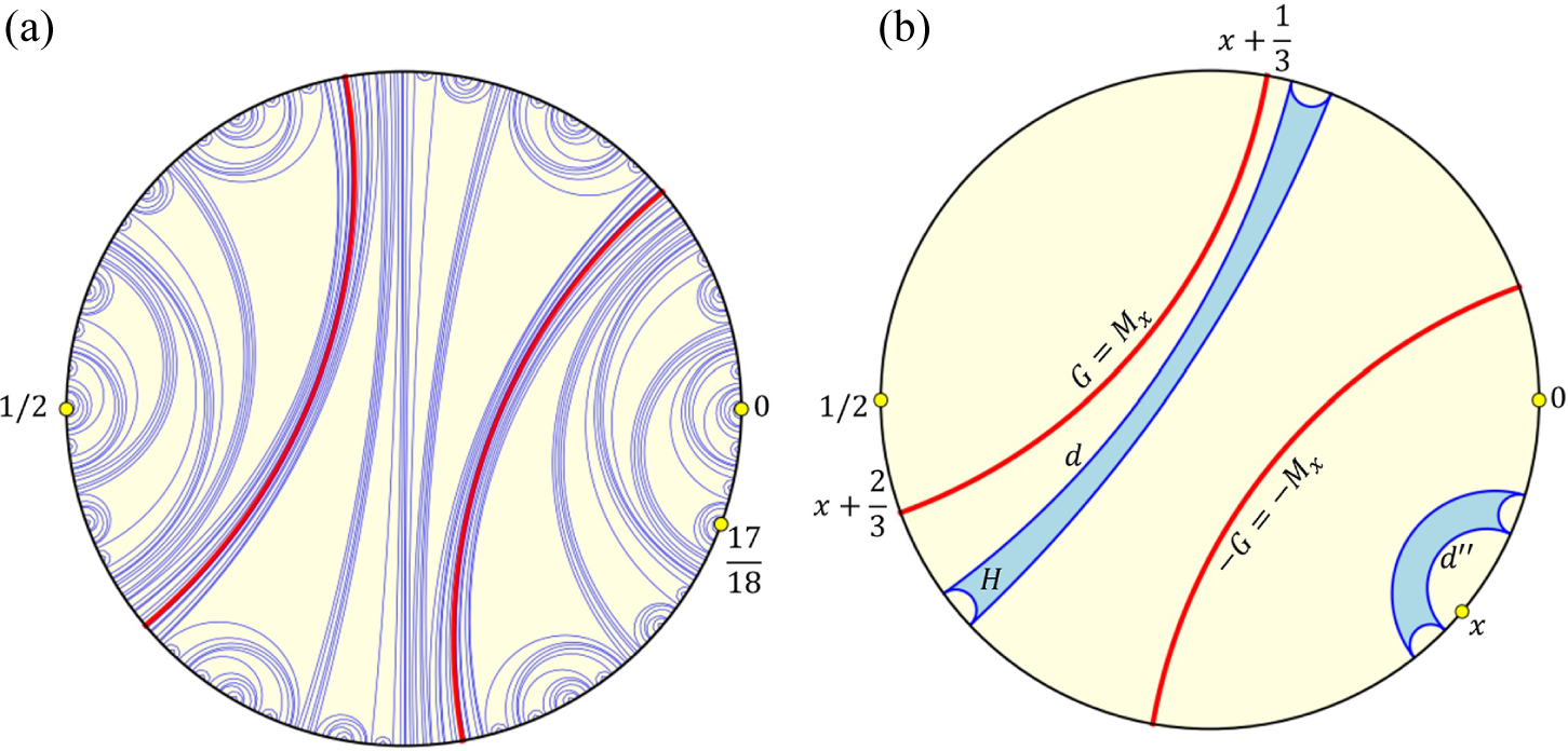
If there are no gaps located close to $M_x$
, then, since
$M_x$
, then, since $\sigma _3$
-periodic points are dense in
$\sigma _3$
-periodic points are dense in $\mathbb {S}$
, we can choose a sequence of periodic leaves of
$\mathbb {S}$
, we can choose a sequence of periodic leaves of $\widehat {\mathcal {L}}$
converging to
$\widehat {\mathcal {L}}$
converging to $M_x$
, and repeat for them the above argument. So, the case when
$M_x$
, and repeat for them the above argument. So, the case when $T=\{x\}$
is a singleton is considered. If T is a leaf/gap, then it is easy to check that any leaf on the boundary of T is legal. Hence, in this case, T is a gap or leaf of
$T=\{x\}$
is a singleton is considered. If T is a leaf/gap, then it is easy to check that any leaf on the boundary of T is legal. Hence, in this case, T is a gap or leaf of $C_sCL$
as desired.
$C_sCL$
as desired.
To prove condition (2), observe that if T is a non-degenerate leaf, then by the above, it is the limit of leaves of $\widehat {\mathcal {L}}$
from both sides. Therefore, it is the limit of pullbacks of
$\widehat {\mathcal {L}}$
from both sides. Therefore, it is the limit of pullbacks of $\pm M_x$
from both sides. Since, under our assumptions, critical leaves
$\pm M_x$
from both sides. Since, under our assumptions, critical leaves $\pm M_x$
are contained in the critical quadrilaterals
$\pm M_x$
are contained in the critical quadrilaterals $\pm G$
, then, in fact pullbacks of
$\pm G$
, then, in fact pullbacks of $\pm G$
accumulate on T from both sides. By definition, it means that leaves of the pullback lamination
$\pm G$
accumulate on T from both sides. By definition, it means that leaves of the pullback lamination $\mathcal {L}(T)$
approach T from both sides. It now follows from Lemmas 4.6 and 4.7 that T is the limit from both sides of comajors disjoint from T as desired.
$\mathcal {L}(T)$
approach T from both sides. It now follows from Lemmas 4.6 and 4.7 that T is the limit from both sides of comajors disjoint from T as desired.
To prove condition (3), observe that, by definition, T has edges that are comajors; then, the desired follows from Lemma 4.9.
Definition 4.14. A preperiodic comajor c of preperiod greater than $1$
or a periodic comajor (necessarily degenerate) is called a Misiurewicz comajor, and any symmetric lamination with a Misiurewicz comajor pair is said to be a Misiurewicz symmetric lamination.
$1$
or a periodic comajor (necessarily degenerate) is called a Misiurewicz comajor, and any symmetric lamination with a Misiurewicz comajor pair is said to be a Misiurewicz symmetric lamination.
We are ready to prove the density of hyperbolicity (Fatou conjecture) for symmetric laminations.
Theorem 4.15. Co-periodic comajors are dense in $C_sCL$
.
$C_sCL$
.
Proof. Consider a non-degenerate comajor $c\in C_sCL$
that is not co-periodic. We have two cases here.
$c\in C_sCL$
that is not co-periodic. We have two cases here.
(a) There is a sequence of leaves $c_i \in \mathcal {L}(c)$
with
$c_i \in \mathcal {L}(c)$
with $c\prec c_i$
and
$c\prec c_i$
and $c_i\rightarrow c$
. Then, by Lemma 4.7, the comajor c is the limit of co-periodic comajors
$c_i\rightarrow c$
. Then, by Lemma 4.7, the comajor c is the limit of co-periodic comajors $\hat {c}_i$
such that
$\hat {c}_i$
such that $c\prec \hat {c}_i$
.
$c\prec \hat {c}_i$
.
(b) A sequence of leaves $c_i\in \mathcal {L}(c)$
converging to c with
$c_i\in \mathcal {L}(c)$
converging to c with $c\prec c_i$
does not exist. Then, c is an edge of a gap G of
$c\prec c_i$
does not exist. Then, c is an edge of a gap G of $\mathcal {L}(c)$
with all vertices of G outside of
$\mathcal {L}(c)$
with all vertices of G outside of $H(c)$
. The lamination
$H(c)$
. The lamination $\mathcal {L}(c)$
has critical quadrilaterals
$\mathcal {L}(c)$
has critical quadrilaterals $\pm Q_c=\pm Q$
. If
$\pm Q_c=\pm Q$
. If $\sigma _3(c)$
eventually maps to an edge of Q, then this edge is periodic, which shows that c is co-periodic, and this is a contradiction with our assumption. Hence,
$\sigma _3(c)$
eventually maps to an edge of Q, then this edge is periodic, which shows that c is co-periodic, and this is a contradiction with our assumption. Hence, $\sigma _3(c)$
never maps to an edge of Q and, therefore, G never maps to a leaf or point. By Theorem 3.9, this implies that G and c are preperiodic of preperiod greater than
$\sigma _3(c)$
never maps to an edge of Q and, therefore, G never maps to a leaf or point. By Theorem 3.9, this implies that G and c are preperiodic of preperiod greater than $1$
(recall that c is not periodic by Lemma 3.17).
$1$
(recall that c is not periodic by Lemma 3.17).
We claim that all edges of G are comajors. Properties of laminations imply that there are two gaps, L and R, attached to $Q_c$
at the appropriate majors of
$Q_c$
at the appropriate majors of $\mathcal {L}(c)$
and such that
$\mathcal {L}(c)$
and such that $\sigma _3(L)=\sigma _3(R)=\sigma _3(G)$
. Now, choose among the edges of G the edge
$\sigma _3(L)=\sigma _3(R)=\sigma _3(G)$
. Now, choose among the edges of G the edge $\ell $
with the greatest length. Then, clearly,
$\ell $
with the greatest length. Then, clearly, $G\cap \mathbb {S}\subset \overline {H(\ell )}$
. Set
$G\cap \mathbb {S}\subset \overline {H(\ell )}$
. Set $M=M_\ell , M'=M^{\prime }_\ell $
. Then, M (or
$M=M_\ell , M'=M^{\prime }_\ell $
. Then, M (or $M'$
) cannot enter the strip S between M and
$M'$
) cannot enter the strip S between M and $M'$
as otherwise, by Proposition 3.8, their images would have to cross edges of
$M'$
as otherwise, by Proposition 3.8, their images would have to cross edges of $L, R,$
or
$L, R,$
or $Q_c$
. This implies that, in fact, any edge d of G is a comajor because
$Q_c$
. This implies that, in fact, any edge d of G is a comajor because $\{d, -d\}$
is legal.
$\{d, -d\}$
is legal.
It follows now that this is exactly the situation described in Lemma 4.13 and that $\mathcal {L}(c)$
gives rise to a laminational equivalence relation
$\mathcal {L}(c)$
gives rise to a laminational equivalence relation $\sim _{\mathcal {L}(c)}$
which, in turn, gives rise to a dendritic q-lamination
$\sim _{\mathcal {L}(c)}$
which, in turn, gives rise to a dendritic q-lamination $\widehat {\mathcal {L}}$
such that G is a gap of
$\widehat {\mathcal {L}}$
such that G is a gap of $\widehat {\mathcal {L}}$
(the last claim follows, e.g., from the fact that, by Theorem 3.22, comajors form a q-lamination). Since there are no isolated leaves in
$\widehat {\mathcal {L}}$
(the last claim follows, e.g., from the fact that, by Theorem 3.22, comajors form a q-lamination). Since there are no isolated leaves in $\widehat {\mathcal {L}}$
, the comajor c is approximated by uncountably many leaves
$\widehat {\mathcal {L}}$
, the comajor c is approximated by uncountably many leaves $\hat {\ell }$
of
$\hat {\ell }$
of $\widehat {\mathcal {L}}$
such that
$\widehat {\mathcal {L}}$
such that $\hat {\ell }\prec c$
. By Lemma 4.6, we may assume that all these leaves of
$\hat {\ell }\prec c$
. By Lemma 4.6, we may assume that all these leaves of $\widehat {\mathcal {L}}$
are comajors. Now, choose a sequence of them that converges to c and satisfy the conditions of case (a) of this proof. By case (a) these leaves are all limits of co-periodic comajors, and hence so is c as desired.
$\widehat {\mathcal {L}}$
are comajors. Now, choose a sequence of them that converges to c and satisfy the conditions of case (a) of this proof. By case (a) these leaves are all limits of co-periodic comajors, and hence so is c as desired.
5 L-algorithm
In this section, we provide an algorithm for constructing all co-periodic comajor leaves. By Theorem 4.15, they are dense in $C_sCL$
, and hence this renders the entire
$C_sCL$
, and hence this renders the entire $C_sCL$
. The algorithm is similar to the famous Lavaurs algorithm for Thurston’s
$C_sCL$
. The algorithm is similar to the famous Lavaurs algorithm for Thurston’s $\mathrm {QML}$
[Reference LavaursLav86, Reference LavaursLav89] (see [Reference Bhattacharya, Blokh and SchleicherBBS21, Reference BhattacharyaBha21] for an extension of this algorithm to the degree d unicritical case). We call it the L-algorithm.
$\mathrm {QML}$
[Reference LavaursLav86, Reference LavaursLav89] (see [Reference Bhattacharya, Blokh and SchleicherBBS21, Reference BhattacharyaBha21] for an extension of this algorithm to the degree d unicritical case). We call it the L-algorithm.
5.1 Preliminaries
Lemma 5.1. [Reference Blokh, Oversteegen, Selinger, Timorin and VejandlaBOSTV1]
A co-periodic comajor leaf is disjoint from all other comajors in $C_sCL$
.
$C_sCL$
.
The following is [Reference Blokh, Oversteegen, Selinger, Timorin and VejandlaBOSTV1, Definition 6.4].
Definition 5.2. Let $\ell $
be a leaf of a symmetric lamination
$\ell $
be a leaf of a symmetric lamination $\mathcal {L}$
and
$\mathcal {L}$
and $k>0$
be such that
$k>0$
be such that ${\sigma _3^k(\ell )\neq \ell }$
(in particular, the leaf
${\sigma _3^k(\ell )\neq \ell }$
(in particular, the leaf $\ell $
is not a diameter). If the leaf
$\ell $
is not a diameter). If the leaf $\sigma _3^k(\ell )$
is under
$\sigma _3^k(\ell )$
is under $\ell $
, then we say that the leaf
$\ell $
, then we say that the leaf $\ell $
moves in by
$\ell $
moves in by $\sigma _3^k$
; if
$\sigma _3^k$
; if $\sigma _3^k(\ell )$
is not under
$\sigma _3^k(\ell )$
is not under $\ell $
, then we say that the leaf
$\ell $
, then we say that the leaf $\ell $
moves out by
$\ell $
moves out by $\sigma _3^k$
. If two leaves
$\sigma _3^k$
. If two leaves $\ell $
and
$\ell $
and $\hat {\ell }$
with
$\hat {\ell }$
with $\ell \prec \hat {\ell }$
of the same lamination both move in or both move out by the map
$\ell \prec \hat {\ell }$
of the same lamination both move in or both move out by the map $\sigma _3^k$
, then we say that the leaves move in the same direction. If one of the leaves
$\sigma _3^k$
, then we say that the leaves move in the same direction. If one of the leaves $\ell $
,
$\ell $
, $\hat {\ell }$
moves in and the other moves out, then we say that the leaves move in opposite directions. There are two ways of moving in opposite directions: if
$\hat {\ell }$
moves in and the other moves out, then we say that the leaves move in opposite directions. There are two ways of moving in opposite directions: if $\ell $
moves out and
$\ell $
moves out and $\hat {\ell }$
moves in, we say they move toward each other; if
$\hat {\ell }$
moves in, we say they move toward each other; if $\ell $
moves in and
$\ell $
moves in and $\hat {\ell }$
moves out, we say that they move away from each other.
$\hat {\ell }$
moves out, we say that they move away from each other.
The strip $\mathcal {S}(\ell , \hat {\ell })$
between non-crossing chords
$\mathcal {S}(\ell , \hat {\ell })$
between non-crossing chords $\ell $
,
$\ell $
, $\hat {\ell }$
was introduced in Definition 3.5.
$\hat {\ell }$
was introduced in Definition 3.5.
Lemma 5.3. [Reference Blokh, Oversteegen, Selinger, Timorin and VejandlaBOSTV1, Lemma 6.5]
Let $\hat {\ell }\neq \ell $
be non-periodic leaves of a symmetric lamination
$\hat {\ell }\neq \ell $
be non-periodic leaves of a symmetric lamination $\mathcal {L}$
with
$\mathcal {L}$
with $\hat {\ell }\succ \ell $
. Given an integer
$\hat {\ell }\succ \ell $
. Given an integer $k>0$
, let
$k>0$
, let $h:\mathbb {S}\to \mathbb {S}$
be either the map
$h:\mathbb {S}\to \mathbb {S}$
be either the map $\sigma _3^k$
or the map
$\sigma _3^k$
or the map $-\sigma _3^k$
. Suppose that the leaves
$-\sigma _3^k$
. Suppose that the leaves $\ell $
and
$\ell $
and $\hat {\ell }$
move toward each other by the map h and neither the leaves
$\hat {\ell }$
move toward each other by the map h and neither the leaves $\ell $
and
$\ell $
and $\hat {\ell }$
, nor any leaf separating them, can eventually map into a leaf (including degenerate) with both endpoints in one of the boundary arcs of the strip
$\hat {\ell }$
, nor any leaf separating them, can eventually map into a leaf (including degenerate) with both endpoints in one of the boundary arcs of the strip $\mathcal {S}(\ell ,\hat {\ell })$
. Then, there exists a
$\mathcal {S}(\ell ,\hat {\ell })$
. Then, there exists a $\sigma _3$
-periodic leaf
$\sigma _3$
-periodic leaf $y\in \mathcal {L}$
that separates
$y\in \mathcal {L}$
that separates $\ell $
and
$\ell $
and $\hat {\ell }$
.
$\hat {\ell }$
.
For the notion of two-sided limit leaves, see Definition 3.16.
Definition 5.4. We say a gap G weakly separates two leaves $\ell _1$
and
$\ell _1$
and $\ell _2$
if
$\ell _2$
if $\ell _1\setminus G$
and
$\ell _1\setminus G$
and $\ell _2\setminus G$
are non-empty sets in two different components of
$\ell _2\setminus G$
are non-empty sets in two different components of $\overline {\mathbb {D}} \setminus G$
. Similarly, we say a leaf
$\overline {\mathbb {D}} \setminus G$
. Similarly, we say a leaf $\ell $
weakly separates two leaves
$\ell $
weakly separates two leaves $\ell _1$
and
$\ell _1$
and $\ell _2$
if
$\ell _2$
if $\ell _1\setminus \ell $
and
$\ell _1\setminus \ell $
and $\ell _2\setminus \ell $
are non-empty sets in two different components of
$\ell _2\setminus \ell $
are non-empty sets in two different components of $\overline {\mathbb {D}} \setminus \ell $
.
$\overline {\mathbb {D}} \setminus \ell $
.
Lemma 5.5. Let $\ell '\neq \ell $
be two leaves in a cubic symmetric lamination
$\ell '\neq \ell $
be two leaves in a cubic symmetric lamination $\mathcal {L}$
such that
$\mathcal {L}$
such that $\ell \prec \ell '$
. Suppose that:
$\ell \prec \ell '$
. Suppose that:
-
(i) the leaves
$\ell $
and
$\ell '$
move away from each other under
$\sigma _3^k$
; -
(ii) no leaf weakly separating
$\ell $
and
$\ell '$
maps to a critical chord of
$\mathbb {S}$
under the map
$\sigma _3^i$
for
$i<k$
.


Then, there exists a periodic leaf $y=\overline {ab}$
with
$y=\overline {ab}$
with $\sigma ^k_3(a)=a,$ $\sigma ^k_3(b)=b$
that weakly separates
$\sigma ^k_3(b)=b$
that weakly separates $\ell $
and
$\ell $
and $\ell '$
.
$\ell '$
.
Proof. A gap G of $\mathcal {L}$
with edges
$\mathcal {L}$
with edges $\ell , \ell '$
does not exist as otherwise, the gap
$\ell , \ell '$
does not exist as otherwise, the gap $\sigma _3^k(G)$
would strictly cover the gap G. Hence, the family of leaves
$\sigma _3^k(G)$
would strictly cover the gap G. Hence, the family of leaves $\mathcal {C}\subset \mathcal {L}$
that consists of
$\mathcal {C}\subset \mathcal {L}$
that consists of $\ell $
,
$\ell $
, $\ell '$
, and the leaves that weakly separate
$\ell '$
, and the leaves that weakly separate $\ell $
and
$\ell $
and $\ell '$
has at least one leaf that weakly separates
$\ell '$
has at least one leaf that weakly separates $\ell $
and
$\ell $
and $\ell '$
. Clearly,
$\ell '$
. Clearly, $\mathcal {C}$
is closed.
$\mathcal {C}$
is closed.
Let A be the set of leaves of $\mathcal {C}$
that move in under
$\mathcal {C}$
that move in under $\sigma _3^k$
such that for every leaf
$\sigma _3^k$
such that for every leaf $m\in A$
, if a leaf n weakly separates
$m\in A$
, if a leaf n weakly separates $\ell $
and m, then n also moves in under the map
$\ell $
and m, then n also moves in under the map $\sigma _3^k$
. So, all the leaves in A move in under
$\sigma _3^k$
. So, all the leaves in A move in under $\sigma _3^k$
. Then, the closure
$\sigma _3^k$
. Then, the closure $\overline {A}$
of A (with respect to the Hausdorff metric) is a family of leaves, too; let
$\overline {A}$
of A (with respect to the Hausdorff metric) is a family of leaves, too; let $y\in \overline {A}$
be the leaf of
$y\in \overline {A}$
be the leaf of $\overline {A}$
farthest from
$\overline {A}$
farthest from $\ell $
(that is, every leaf in
$\ell $
(that is, every leaf in $A\setminus \{\ell , y\}$
weakly separates
$A\setminus \{\ell , y\}$
weakly separates $\ell $
from y). By continuity, either
$\ell $
from y). By continuity, either $y\in A$
or
$y\in A$
or $\sigma _3^k(y)=y$
. We claim that
$\sigma _3^k(y)=y$
. We claim that $\sigma _3^k(y)=y$
. Indeed, suppose that y moves in under
$\sigma _3^k(y)=y$
. Indeed, suppose that y moves in under $\sigma _3^k$
. There are two cases. First, it can be that y is approximated by leaves with endpoints outside
$\sigma _3^k$
. There are two cases. First, it can be that y is approximated by leaves with endpoints outside $H(y)$
(see Definition 3.24). However, this contradicts the choice of y. Second, y can be an edge of a gap G with vertices outside of
$H(y)$
(see Definition 3.24). However, this contradicts the choice of y. Second, y can be an edge of a gap G with vertices outside of $H(y)$
, while all vertices of
$H(y)$
, while all vertices of $\sigma _3^k(G)$
belong to
$\sigma _3^k(G)$
belong to $\overline {H(y)}$
. If now
$\overline {H(y)}$
. If now $\hat {\ell }$
is the edge of G with
$\hat {\ell }$
is the edge of G with $y\prec \hat {\ell }$
, then
$y\prec \hat {\ell }$
, then $\hat {\ell }\in A$
, which is a contradiction.
$\hat {\ell }\in A$
, which is a contradiction.
Thus, $y=\overline {ab}=\sigma _3^k(y)$
. We claim that
$y=\overline {ab}=\sigma _3^k(y)$
. We claim that $\sigma _3^k$
fixes the endpoints of the leaf y. Assume that
$\sigma _3^k$
fixes the endpoints of the leaf y. Assume that $\sigma _3^k$
flips y, and consider cases. If y is a two-sided limit leaf and
$\sigma _3^k$
flips y, and consider cases. If y is a two-sided limit leaf and $t\in A$
is close to y, then the leaf t would move out under
$t\in A$
is close to y, then the leaf t would move out under $\sigma _3^k$
, which is a contradiction. If y is an edge of a gap G, then y is an edge of the gap
$\sigma _3^k$
, which is a contradiction. If y is an edge of a gap G, then y is an edge of the gap $G'=\sigma _3^k(G)$
, the gaps G and
$G'=\sigma _3^k(G)$
, the gaps G and $G'$
are on both sides of the leaf y, and
$G'$
are on both sides of the leaf y, and $\sigma _3^k$
maps one gap to the other. Hence, there is an edge
$\sigma _3^k$
maps one gap to the other. Hence, there is an edge $t\prec y$
of G or
$t\prec y$
of G or $G'$
that belongs to A but moves out under
$G'$
that belongs to A but moves out under $\sigma _3^k$
, which is a contradiction. Finally,
$\sigma _3^k$
, which is a contradiction. Finally, $\sigma _3^k(y)=y$
is non-degenerate.
$\sigma _3^k(y)=y$
is non-degenerate.
Lemma 5.6. [Reference Blokh, Oversteegen, Selinger, Timorin and VejandlaBOSTV1, Lemma 6.3]
Suppose that $\mathcal {L}$
is a cubic symmetric lamination with comajor pair
$\mathcal {L}$
is a cubic symmetric lamination with comajor pair $\{c,-c\}$
and that a short leaf
$\{c,-c\}$
and that a short leaf $\ell _s\in \mathcal {L}$
with
$\ell _s\in \mathcal {L}$
with $c\prec \ell _s$
is such that the leaf
$c\prec \ell _s$
is such that the leaf $\ell _m=\sigma _3(\ell _s)$
never maps under
$\ell _m=\sigma _3(\ell _s)$
never maps under $\pm \ell _m$
. Then, there exists a cubic symmetric lamination
$\pm \ell _m$
. Then, there exists a cubic symmetric lamination $\mathcal {L}(\ell _s)$
with comajor pair
$\mathcal {L}(\ell _s)$
with comajor pair $\{\ell _s,-\ell _s\}$
.
$\{\ell _s,-\ell _s\}$
.
5.2 The description of the L-algorithm
According to [Reference MilnorMil93, Reference Milnor and SchleicherMil09], cubic polynomials with Fatou domains whose first return map is of degree 4 are said to be of type B (Bi-transitive) and cubic polynomials with two cycles of Fatou domains are said to be of type D (Disjoint); in the latter case, first return maps on periodic Fatou domains are, evidently, of degree 2. We classify co-periodic comajors in a similar fashion below. Recall that, by Theorem 4.11, co-periodic comajors c generate hyperbolic q-laminations $\widehat {\mathcal {L}}(c)$
.
$\widehat {\mathcal {L}}(c)$
.
The nature of cubic symmetric laminations gives rise to two notions describing two types of periodic points and related (pre)periodic objects. We give a general definition that applies to all of them. Recall that for $x\in \mathbb {S}$
, we write
$x\in \mathbb {S}$
, we write $-x$
for the point symmetric to x with respect to the center of
$-x$
for the point symmetric to x with respect to the center of $\mathbb {S}$
. Under the identification between
$\mathbb {S}$
. Under the identification between $\mathbb {S}$
and
$\mathbb {S}$
and $\mathbb {R}/\mathbb {Z}$
, the point
$\mathbb {R}/\mathbb {Z}$
, the point $-x$
identifies with
$-x$
identifies with $x+\frac 12$
.
$x+\frac 12$
.
Definition 5.7. (Types B and D)
A $2n$
-periodic point x of
$2n$
-periodic point x of $\sigma _3$
such that
$\sigma _3$
such that $\sigma _3^n(x)=-x$
is said to be of type B. All other periodic points of
$\sigma _3^n(x)=-x$
is said to be of type B. All other periodic points of $\sigma _3$
are said to be of type D. A periodic leaf of a symmetric lamination is of type B if its endpoints are of type B, and of type D otherwise. A co-periodic leaf of a symmetric lamination is of type B if its image is a periodic leaf of type B, and of type D otherwise.
$\sigma _3$
are said to be of type D. A periodic leaf of a symmetric lamination is of type B if its endpoints are of type B, and of type D otherwise. A co-periodic leaf of a symmetric lamination is of type B if its image is a periodic leaf of type B, and of type D otherwise.
Lemma 5.8. [Reference Blokh, Mimbs, Oversteegen and ValkenburgBMOV13, Corollary 3.7]
Suppose that $\ell $
and
$\ell $
and $\hat {\ell }$
are two leaves of a
$\hat {\ell }$
are two leaves of a $\sigma _d$
-invariant lamination that share an endpoint and have non-degenerate distinct images. Then, the orientation of the triple of their endpoints is preserved under the map
$\sigma _d$
-invariant lamination that share an endpoint and have non-degenerate distinct images. Then, the orientation of the triple of their endpoints is preserved under the map $\sigma _d$
.
$\sigma _d$
.
To justify Definition 5.7, we need the next lemma.
Lemma 5.9. A periodic leaf of a symmetric lamination $\mathcal {L}$
cannot have one endpoint of type B and the other endpoint of type D.
$\mathcal {L}$
cannot have one endpoint of type B and the other endpoint of type D.
Proof. Suppose that $\ell =\overline {xy}$
is a periodic leaf of
$\ell =\overline {xy}$
is a periodic leaf of $\mathcal {L}$
such that x is of type B while y is of type D. Then, x is of period
$\mathcal {L}$
such that x is of type B while y is of type D. Then, x is of period $2n$
and
$2n$
and $\sigma _3^n(x)=-x$
. It follows that y is also of period
$\sigma _3^n(x)=-x$
. It follows that y is also of period $2n$
, but
$2n$
, but $\sigma _3^n(y)\ne -y$
. Since
$\sigma _3^n(y)\ne -y$
. Since $\overline {(-x) (\sigma _3^n(y))}=\sigma _3^n(\ell )$
is a leaf of
$\overline {(-x) (\sigma _3^n(y))}=\sigma _3^n(\ell )$
is a leaf of $\mathcal {L}$
, then the leaf
$\mathcal {L}$
, then the leaf $\overline {x (-\sigma _3^n(y))}$
is a leaf of
$\overline {x (-\sigma _3^n(y))}$
is a leaf of $\mathcal {L}$
, too. Thus, the union of leaves
$\mathcal {L}$
, too. Thus, the union of leaves $\ell =\overline {xy}$
and
$\ell =\overline {xy}$
and $\overline {x (-\sigma _3^n(y))}$
is mapped by
$\overline {x (-\sigma _3^n(y))}$
is mapped by $\sigma _3^n$
to the union of leaves
$\sigma _3^n$
to the union of leaves $\overline {(-x) (\sigma _3^n(y))}$
and
$\overline {(-x) (\sigma _3^n(y))}$
and $\overline {(-x) (-y)}$
. However, it is easy to see that the orientation of the triple
$\overline {(-x) (-y)}$
. However, it is easy to see that the orientation of the triple $(y, x, -\sigma _3^n(y))$
is opposite to the orientation of the triple
$(y, x, -\sigma _3^n(y))$
is opposite to the orientation of the triple $(\sigma _3^n(y), -x, -y)$
. This contradicts Lemma 5.8 and completes the proof.
$(\sigma _3^n(y), -x, -y)$
. This contradicts Lemma 5.8 and completes the proof.
Evidently, the $\sigma _3$
-image of an object of type B or D is an object of the same type; co-periodic comajors can be either of type B or of type D. Also, Definition 5.7 allows us to talk about majors, comajors, and minors of types B or D. In the type-B case, a periodic major
$\sigma _3$
-image of an object of type B or D is an object of the same type; co-periodic comajors can be either of type B or of type D. Also, Definition 5.7 allows us to talk about majors, comajors, and minors of types B or D. In the type-B case, a periodic major $M=\overline {ab}$
eventually maps to
$M=\overline {ab}$
eventually maps to $-M$
so that a and b of M eventually map to the
$-M$
so that a and b of M eventually map to the $-a$
and
$-a$
and $-b$
, respectively. In the type-D case, the orbits of a and
$-b$
, respectively. In the type-D case, the orbits of a and $-a$
(and also b and
$-a$
(and also b and $-b$
) are disjoint. Thus, if a co-periodic comajor c is of type B, then the lamination
$-b$
) are disjoint. Thus, if a co-periodic comajor c is of type B, then the lamination $\widehat {\mathcal {L}}(c)$
from Theorem 4.11 has a pair of symmetric Fatou gaps whose first return map is of degree
$\widehat {\mathcal {L}}(c)$
from Theorem 4.11 has a pair of symmetric Fatou gaps whose first return map is of degree $4$
; if c is of type D, then
$4$
; if c is of type D, then $\widehat {\mathcal {L}}(c)$
has a pair of symmetric Fatou gaps whose first return map is of degree 2.
$\widehat {\mathcal {L}}(c)$
has a pair of symmetric Fatou gaps whose first return map is of degree 2.
Definition 5.10. A periodic point (leaf) of type B and period $2n$
is said to be of block period n. A periodic point (leaf) of type D and period n is said to be of block period n. A co-periodic leaf is said to be of block period n if its image is of block period n.
$2n$
is said to be of block period n. A periodic point (leaf) of type D and period n is said to be of block period n. A co-periodic leaf is said to be of block period n if its image is of block period n.
In [Reference Blokh, Oversteegen, Selinger, Timorin and VejandlaBOSTV1], we considered the map $\tau $
that rotates the unit disk by
$\tau $
that rotates the unit disk by $180$
degrees. If
$180$
degrees. If $\mathcal {L}$
is a cubic symmetric lamination, then
$\mathcal {L}$
is a cubic symmetric lamination, then $\tau $
acts on leaves and gaps of
$\tau $
acts on leaves and gaps of $\mathcal {L}$
. We will also interchangeably use the notation
$\mathcal {L}$
. We will also interchangeably use the notation $-\ell $
for
$-\ell $
for $\tau (\ell )$
and
$\tau (\ell )$
and $-G$
for
$-G$
for $\tau (G)$
, where
$\tau (G)$
, where $\ell $
is a leaf of
$\ell $
is a leaf of $\mathcal {L}$
and G is a gap of
$\mathcal {L}$
and G is a gap of $\mathcal {L}$
. Define the map
$\mathcal {L}$
. Define the map $g_j=\tau \circ \sigma _3^j:\mathcal {L} \rightarrow \mathcal {L}$
for some j. Lemma 5.11 is similar to Lemma 5.5. We state it without proof.
$g_j=\tau \circ \sigma _3^j:\mathcal {L} \rightarrow \mathcal {L}$
for some j. Lemma 5.11 is similar to Lemma 5.5. We state it without proof.
Lemma 5.11. Let $\ell '\neq \ell $
be two leaves in a cubic symmetric lamination
$\ell '\neq \ell $
be two leaves in a cubic symmetric lamination $\mathcal {L}$
such that
$\mathcal {L}$
such that $\ell \prec \ell '$
. Suppose that:
$\ell \prec \ell '$
. Suppose that:
-
(i) the leaves
$\ell $
and
$\ell '$
move away from each other under
$g_k$
; -
(ii) no leaf weakly separating
$\ell $
and
$\ell '$
maps to a critical chord of
$\mathbb {S}$
under the map
$g_i$
for
$i<k$
.


Then, there exists a periodic leaf y of period $1$
under the map
$1$
under the map $g_k$
that weakly separates
$g_k$
that weakly separates $\ell $
and
$\ell $
and $\ell '$
.
$\ell '$
.
The next lemma deals with dynamics of comajors.
Lemma 5.12. Suppose that $c'\prec c$
are distinct co-periodic comajors that are leaves of a lamination
$c'\prec c$
are distinct co-periodic comajors that are leaves of a lamination $\mathcal {L}$
. Then, there is no finite gap H of
$\mathcal {L}$
. Then, there is no finite gap H of $\mathcal {L}$
such that both
$\mathcal {L}$
such that both $c'$
and c are edges of H.
$c'$
and c are edges of H.
Proof. The leaves $m'=\sigma _3(c')\prec m = \sigma _3(c)$
are periodic. By way of contradiction, assume that both are edges of a periodic gap
$m'=\sigma _3(c')\prec m = \sigma _3(c)$
are periodic. By way of contradiction, assume that both are edges of a periodic gap $\sigma _3(H)=G$
of
$\sigma _3(H)=G$
of $\mathcal {L}$
. Then, their endpoints stay in the same circular order along their periodic orbits. By Lemma 3.10, if G is 1-rotational, then the leaf m will eventually map to the leaf
$\mathcal {L}$
. Then, their endpoints stay in the same circular order along their periodic orbits. By Lemma 3.10, if G is 1-rotational, then the leaf m will eventually map to the leaf $m'$
, and if G is 2-rotational, then the leaf m will eventually map to the leaf
$m'$
, and if G is 2-rotational, then the leaf m will eventually map to the leaf $-m'$
, in either case, contradicting that m is the shortest leaf in its orbit (see Lemma 3.15).
$-m'$
, in either case, contradicting that m is the shortest leaf in its orbit (see Lemma 3.15).
Now, the main theorem needed for the L-algorithm is as follows.
Theorem 5.13. Suppose that co-periodic comajors c and $c'$
have the following properties:
$c'$
have the following properties:
-
(i)
$c'\prec c$
; -
(ii) both c and
$c'$
are either of type B or type D; and -
(iii) c and
$c'$
have the same block period n.


Then, there exists a co-periodic comajor d with $c'\prec d\prec c$
such that d is of block period
$c'\prec d\prec c$
such that d is of block period $j<n$
.
$j<n$
.
Proof. Choose a preperiodic point p of preperiod bigger than 1 and period bigger than n in the arc $H(c')$
. By Lemma 4.13, there exists a cubic symmetric dendritic q-lamination
$H(c')$
. By Lemma 4.13, there exists a cubic symmetric dendritic q-lamination $\mathcal {L}$
with a pair of finite critical gaps/leaves
$\mathcal {L}$
with a pair of finite critical gaps/leaves $\{\Delta ,-\Delta \}$
such that
$\{\Delta ,-\Delta \}$
such that $\sigma _3(p)\in \sigma _3(\Delta )$
(that is, the critical leaves
$\sigma _3(p)\in \sigma _3(\Delta )$
(that is, the critical leaves $\pm \ell $
of
$\pm \ell $
of $\mathcal {L}(p)$
are contained in the critical sets
$\mathcal {L}(p)$
are contained in the critical sets $\Delta $
and
$\Delta $
and $-\Delta $
), iterated preimages of
$-\Delta $
), iterated preimages of $\pm \ell $
converge to all sides of
$\pm \ell $
converge to all sides of $\Delta $
and
$\Delta $
and $-\Delta $
, so that pullbacks of the critical sets are dense in
$-\Delta $
, so that pullbacks of the critical sets are dense in $\mathcal {L}$
, and c and
$\mathcal {L}$
, and c and $c'$
are leaves of
$c'$
are leaves of $\mathcal {L}$
. The leaves
$\mathcal {L}$
. The leaves $m = \sigma _3(c)$
and
$m = \sigma _3(c)$
and $m'=\sigma _3(c')$
are periodic and such that
$m'=\sigma _3(c')$
are periodic and such that $m'\prec m$
. Since preimages of
$m'\prec m$
. Since preimages of $\pm \Delta $
are dense in
$\pm \Delta $
are dense in $\mathcal {L}$
, then it follows from Lemma 5.12 that for a minimal k, the set
$\mathcal {L}$
, then it follows from Lemma 5.12 that for a minimal k, the set $\Delta $
(or
$\Delta $
(or $-\Delta $
) separates
$-\Delta $
) separates $\sigma _3^k(m)$
and
$\sigma _3^k(m)$
and $\sigma _3^k(m')$
. Consider cases.
$\sigma _3^k(m')$
. Consider cases.
(i) comajors c and $c'$
are of type D. Then, the periodic orbits of m and
$c'$
are of type D. Then, the periodic orbits of m and $-m$
(and also
$-m$
(and also $m'$
and
$m'$
and $-m'$
) are disjoint and have period n. We claim that
$-m'$
) are disjoint and have period n. We claim that $k\ne n-1$
. If
$k\ne n-1$
. If $k=n-1$
, then
$k=n-1$
, then $\sigma _3^{k}(m)$
and
$\sigma _3^{k}(m)$
and $\sigma _3^{k}(m')$
are long/medium siblings of c and
$\sigma _3^{k}(m')$
are long/medium siblings of c and $c'$
, respectively. Hence, they must be separated by
$c'$
, respectively. Hence, they must be separated by $\Delta $
. The circular order of the four endpoints of m and
$\Delta $
. The circular order of the four endpoints of m and $m'$
is preserved in the leaves
$m'$
is preserved in the leaves $\sigma _3^{n-1}(m)$
and
$\sigma _3^{n-1}(m)$
and $\sigma _3^{n-1}(m')$
, but when
$\sigma _3^{n-1}(m')$
, but when $\sigma _3$
is applied one more time, exactly one of the leaves
$\sigma _3$
is applied one more time, exactly one of the leaves $\sigma _3^{n-1}(m)$
and
$\sigma _3^{n-1}(m)$
and $\sigma _3^{n-1}(m')$
flips because of the critical gap between them. Hence, the order among the endpoints of
$\sigma _3^{n-1}(m')$
flips because of the critical gap between them. Hence, the order among the endpoints of $\sigma _3^n(m)=m$
and
$\sigma _3^n(m)=m$
and $\sigma _3^n(m')=m'$
cannot be the same as the order among the endpoints of m and
$\sigma _3^n(m')=m'$
cannot be the same as the order among the endpoints of m and $m'$
, which is absurd. Thus,
$m'$
, which is absurd. Thus, $0\le k<n-1$
.
$0\le k<n-1$
.
(a) it is $\Delta $
that separates the leaves
$\Delta $
that separates the leaves $\sigma _3^k(m)$
and
$\sigma _3^k(m)$
and $\sigma _3^k(m')$
. Since the leaves and gaps separating m and
$\sigma _3^k(m')$
. Since the leaves and gaps separating m and $m'$
map one-to-one under
$m'$
map one-to-one under $\sigma _3^k$
, there is a set
$\sigma _3^k$
, there is a set $\Delta ^{\ast }$
separating m and
$\Delta ^{\ast }$
separating m and $m'$
with
$m'$
with $\sigma _3^k(\Delta ^{\ast })=\Delta $
. Moreover, since
$\sigma _3^k(\Delta ^{\ast })=\Delta $
. Moreover, since $\sigma _3(p)\prec m'$
,
$\sigma _3(p)\prec m'$
, $\sigma _3^{k+1}(\Delta ^{\ast })=\sigma _3(\Delta )\prec m'$
(see Figure 8). Let
$\sigma _3^{k+1}(\Delta ^{\ast })=\sigma _3(\Delta )\prec m'$
(see Figure 8). Let $\ell ^{\ast }$
be the side of
$\ell ^{\ast }$
be the side of $\Delta ^{\ast }$
that separates m and
$\Delta ^{\ast }$
that separates m and $m'$
and is closest to the leaf m. Then,
$m'$
and is closest to the leaf m. Then, $\ell ^{\ast }$
moves in under the map
$\ell ^{\ast }$
moves in under the map $\sigma _3^{k+1}$
. However, the leaf
$\sigma _3^{k+1}$
. However, the leaf $\sigma _3^{k+1}(m)$
is neither under the leaf m nor under the leaf
$\sigma _3^{k+1}(m)$
is neither under the leaf m nor under the leaf $-m$
because the minor is the shortest leaf in its orbit. Hence, the leaves m and
$-m$
because the minor is the shortest leaf in its orbit. Hence, the leaves m and $\ell ^{\ast }$
move away from each other under the map
$\ell ^{\ast }$
move away from each other under the map $\sigma _3^{k+1}$
.
$\sigma _3^{k+1}$
.

Let us verify condition (2) from Lemma 5.5. Note that $\sigma _3^k(\ell ^{\ast })=M$
is a major of
$\sigma _3^k(\ell ^{\ast })=M$
is a major of $\mathcal {L}$
. For
$\mathcal {L}$
. For $i\le k$
, the map
$i\le k$
, the map $\sigma _3^i$
takes the leaves separating
$\sigma _3^i$
takes the leaves separating $\ell ^{\ast }$
and m in the strip
$\ell ^{\ast }$
and m in the strip $\mathcal {S}(\ell ^{\ast }, m)$
one-to-one to the leaves separating
$\mathcal {S}(\ell ^{\ast }, m)$
one-to-one to the leaves separating $\sigma _3^i(\ell ^*)$
and
$\sigma _3^i(\ell ^*)$
and $\sigma _3^i(m)$
in the strip
$\sigma _3^i(m)$
in the strip $\mathcal {S}(\sigma _3^i(\ell ^*),\sigma _3^i(m))$
. As there are no critical chords of
$\mathcal {S}(\sigma _3^i(\ell ^*),\sigma _3^i(m))$
. As there are no critical chords of $\mathbb {S}$
in
$\mathbb {S}$
in $\mathcal {S}(\sigma _3^i(\ell ^*),\sigma _3^i(m))$
for
$\mathcal {S}(\sigma _3^i(\ell ^*),\sigma _3^i(m))$
for $i<k$
, no leaf separating
$i<k$
, no leaf separating $\ell ^{\ast }$
and m maps to a critical chord of
$\ell ^{\ast }$
and m maps to a critical chord of $\mathbb {S}$
under the map
$\mathbb {S}$
under the map $\sigma _3^i$
for
$\sigma _3^i$
for $i< k$
. Moreover, if
$i< k$
. Moreover, if $i=k$
, then all such leaves are situated between
$i=k$
, then all such leaves are situated between $\Delta $
and M and, hence, can also not be critical. Hence, by Lemma 5.5, there is a periodic leaf
$\Delta $
and M and, hence, can also not be critical. Hence, by Lemma 5.5, there is a periodic leaf $y\in \mathcal {L}$
of period
$y\in \mathcal {L}$
of period $k+1<n$
separating m and
$k+1<n$
separating m and $\ell ^{\ast }$
.
$\ell ^{\ast }$
.
Let $\mathcal {C}$
be the collection of leaves separating m and
$\mathcal {C}$
be the collection of leaves separating m and $m'$
. Let
$m'$
. Let $C_1$
be the collection of all
$C_1$
be the collection of all $\sigma _3$
-periodic leaves in
$\sigma _3$
-periodic leaves in $\mathcal {C}$
of period smaller than n. Let
$\mathcal {C}$
of period smaller than n. Let $C_2$
be the collection of all fixed leaves under the maps
$C_2$
be the collection of all fixed leaves under the maps $g_i=-\sigma _3^i$
,
$g_i=-\sigma _3^i$
, $0<i<n$
in
$0<i<n$
in $\mathcal {C}$
; we associate the minimal such i with all leaves from
$\mathcal {C}$
; we associate the minimal such i with all leaves from $C_2$
. Since
$C_2$
. Since $y\in C_1$
, then
$y\in C_1$
, then $C_1\ne \varnothing $
, but
$C_1\ne \varnothing $
, but $C_2$
could be empty.
$C_2$
could be empty.
Let $y_1$
be a leaf of the least period
$y_1$
be a leaf of the least period $j_1\le k+1<n$
in
$j_1\le k+1<n$
in $C_1$
. Choose
$C_1$
. Choose $y_1$
to be the closest to m among leaves of
$y_1$
to be the closest to m among leaves of $C_1$
of period
$C_1$
of period $j_1$
. Similarly, choose a
$j_1$
. Similarly, choose a $-\sigma _3^{j_2}$
-fixed leaf
$-\sigma _3^{j_2}$
-fixed leaf $y_2$
in
$y_2$
in $C_2$
such that
$C_2$
such that $j_2$
is the smallest possible; choose
$j_2$
is the smallest possible; choose $y_2$
to be the closest to m among
$y_2$
to be the closest to m among $-\sigma _3^{j_2}$
-fixed leaves in
$-\sigma _3^{j_2}$
-fixed leaves in $C_2$
. If
$C_2$
. If $j_1\leq j_2$
, then we claim that the leaf d, which is the short pullback of
$j_1\leq j_2$
, then we claim that the leaf d, which is the short pullback of $y_1$
in
$y_1$
in $\mathcal {L}$
, is the desired comajor of block period
$\mathcal {L}$
, is the desired comajor of block period $j=j_1<n$
(recall that
$j=j_1<n$
(recall that $y_1$
is located between the minors m and
$y_1$
is located between the minors m and $m'$
). By Lemma 5.6, it suffices to prove that the leaf
$m'$
). By Lemma 5.6, it suffices to prove that the leaf $y_1$
neither maps under itself nor under the leaf
$y_1$
neither maps under itself nor under the leaf $-y_1$
under the map
$-y_1$
under the map $\sigma _3^i$
for any
$\sigma _3^i$
for any $i<j_1$
.
$i<j_1$
.
(1) If $y_1$
maps under itself under
$y_1$
maps under itself under $\sigma _3^i$
for some
$\sigma _3^i$
for some $i<j_1$
, then the leaves
$i<j_1$
, then the leaves $y_1$
and m move away from each other under
$y_1$
and m move away from each other under $\sigma _3^i$
. By Lemma 5.5, there is a
$\sigma _3^i$
. By Lemma 5.5, there is a $\sigma _3$
-periodic leaf
$\sigma _3$
-periodic leaf $y_1'$
of period
$y_1'$
of period $i<j_1$
separating m and
$i<j_1$
separating m and $y_1$
; which is a contradiction with the minimality of
$y_1$
; which is a contradiction with the minimality of $j_1$
.
$j_1$
.
(2) If $y_1$
maps under
$y_1$
maps under $-y_1$
under
$-y_1$
under $\sigma _3^i$
for some
$\sigma _3^i$
for some $i<j_1$
, then the leaf
$i<j_1$
, then the leaf $g_i(y_1)$
is under the leaf
$g_i(y_1)$
is under the leaf $y_1$
. Now, the leaves
$y_1$
. Now, the leaves $y_1$
and m move away from each other under
$y_1$
and m move away from each other under $g_i=-\sigma _3^i$
. By Lemma 5.11, there is a
$g_i=-\sigma _3^i$
. By Lemma 5.11, there is a $-\sigma _3^i$
-fixed leaf
$-\sigma _3^i$
-fixed leaf $y_1'$
that separates m and
$y_1'$
that separates m and $y_1$
. Clearly,
$y_1$
. Clearly, $y_1'$
separates m and
$y_1'$
separates m and $m'$
, too. Then,
$m'$
, too. Then, $i<j_1\le j_2$
is the block period associated with
$i<j_1\le j_2$
is the block period associated with $y_1$
, which contradicts the choice of
$y_1$
, which contradicts the choice of $j_2$
.
$j_2$
.
Thus, the short pullback d of $y_1$
in
$y_1$
in $\mathcal {L}$
is the desired comajor of block period
$\mathcal {L}$
is the desired comajor of block period $j=j_1<n$
. Similarly, if
$j=j_1<n$
. Similarly, if $j_2<j_1$
, then we obtain that the short pullback d of
$j_2<j_1$
, then we obtain that the short pullback d of $y_2$
in
$y_2$
in $\mathcal {L}$
is the desired comajor of block period
$\mathcal {L}$
is the desired comajor of block period $j=j_2<n$
.
$j=j_2<n$
.
(b) it is $-\Delta $
that separates the leaves
$-\Delta $
that separates the leaves $\sigma _3^k(m)$
and
$\sigma _3^k(m)$
and $\sigma _3^k(m')$
, not
$\sigma _3^k(m')$
, not $\Delta $
. We use the arguments from case (a) and find a gap
$\Delta $
. We use the arguments from case (a) and find a gap $\Delta ^{\ast }$
with
$\Delta ^{\ast }$
with $\sigma _3^{k}(\Delta ^{\ast })=-\Delta $
separating m and
$\sigma _3^{k}(\Delta ^{\ast })=-\Delta $
separating m and $m'$
. Then, we have the gap
$m'$
. Then, we have the gap $\sigma _3^{k+1}(\Delta ^{\ast })$
going under the leaf
$\sigma _3^{k+1}(\Delta ^{\ast })$
going under the leaf $-m'$
. The only difference in the arguments is that we use Lemma 5.11 first to find a leaf y separating m and
$-m'$
. The only difference in the arguments is that we use Lemma 5.11 first to find a leaf y separating m and $m'$
such that
$m'$
such that $g_{k+1}(y)=y$
. Thus, the collection
$g_{k+1}(y)=y$
. Thus, the collection $C_2$
is non-empty here, whereas collection
$C_2$
is non-empty here, whereas collection $C_1$
could be empty. The rest of the argument follows exactly as before and we end up with a comajor d between c and
$C_1$
could be empty. The rest of the argument follows exactly as before and we end up with a comajor d between c and $c'$
of a block period
$c'$
of a block period $j<n$
.
$j<n$
.
(ii) comajors c and $c'$
are of type B. The leaves m and
$c'$
are of type B. The leaves m and $m'$
are now periodic of period
$m'$
are now periodic of period $p=2n$
and have symmetric orbits (the orbits of m and
$p=2n$
and have symmetric orbits (the orbits of m and $-m$
are the same). Similarly, the orbits of the leaves
$-m$
are the same). Similarly, the orbits of the leaves $m'$
and
$m'$
and $-m'$
are the same as well. In this case, the proof is very similar to that of case (i) (see Figure 8).
$-m'$
are the same as well. In this case, the proof is very similar to that of case (i) (see Figure 8).
First, we show that there exists an integer k with $0\le k<n-1$
such that
$0\le k<n-1$
such that $\Delta $
or
$\Delta $
or $-\Delta $
separates the leaves
$-\Delta $
separates the leaves $\sigma _3^k(m)$
and
$\sigma _3^k(m)$
and $\sigma _3^k(m')$
. Indeed, let k be the smallest integer between
$\sigma _3^k(m')$
. Indeed, let k be the smallest integer between $0$
and
$0$
and $p=2n$
such that the leaves
$p=2n$
such that the leaves $\sigma _3^k(m)$
and
$\sigma _3^k(m)$
and $\sigma _3^k(m')$
are separated by a critical gap/leaf. As the orbits of both the leaves m and
$\sigma _3^k(m')$
are separated by a critical gap/leaf. As the orbits of both the leaves m and $m'$
are symmetric, the strips formed by the leaves
$m'$
are symmetric, the strips formed by the leaves $\sigma _3^i(m)$
and
$\sigma _3^i(m)$
and $\sigma _3^i(m')$
, where
$\sigma _3^i(m')$
, where $0<i\leq n-1$
, are symmetric to the strips formed by the leaves
$0<i\leq n-1$
, are symmetric to the strips formed by the leaves $\sigma _3^r(m)$
and
$\sigma _3^r(m)$
and $\sigma _3^r(m')$
, where
$\sigma _3^r(m')$
, where $n\leq r<2n$
. It follows that, for the first time, the separation by one of the critical gaps/leaves
$n\leq r<2n$
. It follows that, for the first time, the separation by one of the critical gaps/leaves $\Delta $
and
$\Delta $
and $-\Delta $
happens during the first half of the cycle, that is,
$-\Delta $
happens during the first half of the cycle, that is, $0\le k\leq n-1$
.
$0\le k\leq n-1$
.
To see that k cannot be equal to $n-1$
, assume the contrary. Since
$n-1$
, assume the contrary. Since $\sigma _3^n(m)=-m$
and
$\sigma _3^n(m)=-m$
and $\sigma _3^n(m')=-m'$
, the leaves
$\sigma _3^n(m')=-m'$
, the leaves $\sigma _3^{n-1}(m)$
and
$\sigma _3^{n-1}(m)$
and $\sigma _3^{n-1}(m')$
must be long/medium siblings of
$\sigma _3^{n-1}(m')$
must be long/medium siblings of $-c$
and
$-c$
and $-c'$
, respectively. Hence, they are separated by
$-c'$
, respectively. Hence, they are separated by $-\Delta $
. The circular order of the four endpoints of m and
$-\Delta $
. The circular order of the four endpoints of m and $m'$
is preserved in the leaves
$m'$
is preserved in the leaves $\sigma _3^{n-1}(m)$
and
$\sigma _3^{n-1}(m)$
and $\sigma _3^{n-1}(m')$
, and exactly one of them flips under the next iteration because of a critical gap between them. Without loss of generality, assume that the leaf
$\sigma _3^{n-1}(m')$
, and exactly one of them flips under the next iteration because of a critical gap between them. Without loss of generality, assume that the leaf $\sigma _3^{n-1}(m)$
flips its endpoints when it maps to the leaf
$\sigma _3^{n-1}(m)$
flips its endpoints when it maps to the leaf $-m=\sigma _3^n(m)$
. Since no additional flip takes place under the remaining part of the orbit, it would follow that m returns to itself under
$-m=\sigma _3^n(m)$
. Since no additional flip takes place under the remaining part of the orbit, it would follow that m returns to itself under $\sigma _3^{2n}$
with its endpoints flipped, which is a contradiction. Thus,
$\sigma _3^{2n}$
with its endpoints flipped, which is a contradiction. Thus, $0<k<n-1$
. We have two subcases here similar to case (i).
$0<k<n-1$
. We have two subcases here similar to case (i).
(a) it is $\Delta $
that separates the leaves
$\Delta $
that separates the leaves $\sigma _3^k(m)$
and
$\sigma _3^k(m)$
and $\sigma _3^k(m')$
. Then, following the similar arguments as in case (i)(a), we find a comajor d of block period
$\sigma _3^k(m')$
. Then, following the similar arguments as in case (i)(a), we find a comajor d of block period $j<k+1=n$
separating the leaves c and
$j<k+1=n$
separating the leaves c and $c'$
.
$c'$
.
(b) it is $-\Delta $
that separates the leaves
$-\Delta $
that separates the leaves $\sigma _3^k(m)$
and
$\sigma _3^k(m)$
and $\sigma _3^k(m')$
, not
$\sigma _3^k(m')$
, not $\Delta $
. Then, using similar arguments to case (i)(b), we find a comajor d of block period
$\Delta $
. Then, using similar arguments to case (i)(b), we find a comajor d of block period $j<k+1=n$
separating the leaves c and
$j<k+1=n$
separating the leaves c and $c'$
.
$c'$
.
Theorem 5.13 allows us to describe an algorithm for finding co-periodic cubic comajors similar to the Lavaurs algorithm [Reference LavaursLav86, Reference LavaursLav89] for finding periodic quadratic minors. We call this algorithm the L-algorithm.
L-algorithm
Draw co-periodic comajors of block period $1$
. It is easy to verify that type-D co-periodic comajors of period 1 are
$1$
. It is easy to verify that type-D co-periodic comajors of period 1 are $\overline {\tfrac 16\tfrac 13}$
and
$\overline {\tfrac 16\tfrac 13}$
and $\overline {\tfrac 23\tfrac 56}$
. Similarly, type-B co-periodic comajors of block period
$\overline {\tfrac 23\tfrac 56}$
. Similarly, type-B co-periodic comajors of block period $1$
are
$1$
are $\overline {\tfrac {5}{12} \tfrac {7}{12}}$
and
$\overline {\tfrac {5}{12} \tfrac {7}{12}}$
and $\overline {\tfrac {11}{12}\tfrac {1}{12}}$
.
$\overline {\tfrac {11}{12}\tfrac {1}{12}}$
.
We proceed by induction. Suppose that all preperiodic comajors of block periods from $1$
to k (inclusively) have been drawn. Denote the family of them by
$1$
to k (inclusively) have been drawn. Denote the family of them by $\mathcal {F}_k$
. Consider a component A of
$\mathcal {F}_k$
. Consider a component A of $\overline {\mathbb {D}} \setminus \bigcup _{\ell \in \mathcal {F}_n} \ell $
. Then, there are two cases.
$\overline {\mathbb {D}} \setminus \bigcup _{\ell \in \mathcal {F}_n} \ell $
. Then, there are two cases.
(a) Suppose that there is a comajor $\ell _0$
such that all points of A are located under
$\ell _0$
such that all points of A are located under $\ell _0$
. Then, there may be several comajors
$\ell _0$
. Then, there may be several comajors $\ell _1$
,
$\ell _1$
, $\ldots ,$ $\ell _s$
located under
$\ell _s$
located under $\ell _0$
with endpoints in
$\ell _0$
with endpoints in ${A\cap \mathbb {S}}$
(this collection of comajors may be empty). Consider the set
${A\cap \mathbb {S}}$
(this collection of comajors may be empty). Consider the set $B=\{b_1<\cdots <b_t\}$
of preperiodic points of type B of preperiod 1 and block period
$B=\{b_1<\cdots <b_t\}$
of preperiodic points of type B of preperiod 1 and block period $k+1$
that belong to
$k+1$
that belong to $A\cap \mathbb {S}$
. These points (if any) must be connected to create several comajors. By Lemma 5.1, these comajors are pairwise disjoint. By Theorem 5.13, no two comajors from that collection can be located so that one of them is under the other one. Hence,
$A\cap \mathbb {S}$
. These points (if any) must be connected to create several comajors. By Lemma 5.1, these comajors are pairwise disjoint. By Theorem 5.13, no two comajors from that collection can be located so that one of them is under the other one. Hence, $t=2r$
is even and the comajors in question are
$t=2r$
is even and the comajors in question are $\overline {b_1b_2}$
,
$\overline {b_1b_2}$
, $\ldots ,$ $\overline {b_{2r-1}b_{2r}}$
. We can also consider the set D of preperiodic points of type D of preperiod 1 and block period
$\overline {b_{2r-1}b_{2r}}$
. We can also consider the set D of preperiodic points of type D of preperiod 1 and block period $k+1$
that belong to
$k+1$
that belong to $A\cap \mathbb {S}$
. These points should be connected similar to how points from B were connected, that is, consecutively.
$A\cap \mathbb {S}$
. These points should be connected similar to how points from B were connected, that is, consecutively.
Do this for all components A for which there is a comajor $\ell _0$
such that all points of A are located under
$\ell _0$
such that all points of A are located under $\ell _0$
.
$\ell _0$
.
(b) There is exactly one component C of $\overline {\mathbb {D}} \setminus \bigcup _{\ell \in \mathcal {F}_n} \ell $
for which there is no comajor
$\overline {\mathbb {D}} \setminus \bigcup _{\ell \in \mathcal {F}_n} \ell $
for which there is no comajor $\ell _0$
with all points of A located under
$\ell _0$
with all points of A located under $\ell _0$
. This is the ‘central’ component left after the closures of all components described in case (a) are removed from
$\ell _0$
. This is the ‘central’ component left after the closures of all components described in case (a) are removed from $\mathbb {D}$
. Evidently, this component contains the center of
$\mathbb {D}$
. Evidently, this component contains the center of $\overline {\mathbb {D}}$
and is unique.
$\overline {\mathbb {D}}$
and is unique.
As before, let B be the set of preperiodic points of type B of preperiod 1 and block period $k+1$
that belong to
$k+1$
that belong to $C\cap \mathbb {S}$
. However, unlike before, let us divide B into four subsets:
$C\cap \mathbb {S}$
. However, unlike before, let us divide B into four subsets: $B^1=B\cap (1/{12}, \frac 16)$
,
$B^1=B\cap (1/{12}, \frac 16)$
, $B^2=B\cap (\frac 13, 5/{12})$
,
$B^2=B\cap (\frac 13, 5/{12})$
, $B_3=B\cap (7/{12}, \frac 23),$
and
$B_3=B\cap (7/{12}, \frac 23),$
and ${B_4=B\cap (\tfrac 56, {11}/{12})}$
. Since comajors are short, a comajor cannot connect two points from two distinct B-sets. Hence, as in case (a), comajors connect points from B consecutively within B-sets. If, e.g.,
${B_4=B\cap (\tfrac 56, {11}/{12})}$
. Since comajors are short, a comajor cannot connect two points from two distinct B-sets. Hence, as in case (a), comajors connect points from B consecutively within B-sets. If, e.g., $B_1=\{b_1<\cdots <b_t\}$
, then, as in case (a),
$B_1=\{b_1<\cdots <b_t\}$
, then, as in case (a), $t=2r$
is even, and the corresponding comajors are
$t=2r$
is even, and the corresponding comajors are $\overline {b_1b_2}$
,
$\overline {b_1b_2}$
, $\ldots $
,
$\ldots $
, $\overline {b_{2r-1}b_{2r}}$
. Points of type D that belong to
$\overline {b_{2r-1}b_{2r}}$
. Points of type D that belong to $\partial C$
should be treated similarly.
$\partial C$
should be treated similarly.
Thus, the L-algorithm for cubic symmetric laminations is as follows. First, we take step 1 and draw the comajors $\overline {\tfrac {11}{12}\tfrac {1}{12}},$ $\overline {\tfrac 16\tfrac 13}$
,
$\overline {\tfrac 16\tfrac 13}$
, $\overline {\tfrac {5}{12}\tfrac {7}{12}},$
and
$\overline {\tfrac {5}{12}\tfrac {7}{12}},$
and $\overline {\tfrac 23\tfrac 56}.$
Then, on each next step, say,
$\overline {\tfrac 23\tfrac 56}.$
Then, on each next step, say, $k+1,$
we first plot all type-B points of preperiod 1 and block period
$k+1,$
we first plot all type-B points of preperiod 1 and block period $k+1$
and connect them consecutively, starting from the smallest positive angle. Then, we plot all type-D points of preperiod 1 and block period
$k+1$
and connect them consecutively, starting from the smallest positive angle. Then, we plot all type-D points of preperiod 1 and block period $k+1$
, and connect them consecutively, too, starting from the smallest positive angle.
$k+1$
, and connect them consecutively, too, starting from the smallest positive angle.
Acknowledgments
The results of this paper were reported by the authors at the Lamination Seminar at UAB. It is a pleasure to express our gratitude to the members of the seminar for their useful remarks and suggestions. We are also very grateful to the referees for thoughtful and useful remarks that helped us significantly improve the exposition of the paper. A.B. was partially supported by NSF grant DMS-2349942. L.G.O. was partially supported by NSF grant DMS-1807558. V.T. was partially supported by the HSE University Basic Research Program. Theorem 4.11 was supported by the Russian Science Foundation under grant no. 22-11-00177.


 Open access