


1 Introduction
Phase resetting is a technique that is often applied in neuroscience to study the behaviour and properties of neuronal firing patterns [Reference Ermentrout and Terman4, Reference Schultheiss, Prinz and Butera18]. In essence, given a stable oscillation, denoted $\Gamma $
, a phase reset is the act of applying a perturbation of a particular strength, in a particular direction, and recording the resulting phase shift upon return to
$\Gamma $
, a phase reset is the act of applying a perturbation of a particular strength, in a particular direction, and recording the resulting phase shift upon return to $\Gamma $
with respect to the phase at which the perturbation was applied. Phase resetting is strongly related to the notion of isochrons, which each comprise all points that converge to
$\Gamma $
with respect to the phase at which the perturbation was applied. Phase resetting is strongly related to the notion of isochrons, which each comprise all points that converge to $\Gamma $
with a given phase: the phase reset maps a point on
$\Gamma $
with a given phase: the phase reset maps a point on $\Gamma $
to a perturbed point that lies on a particular isochron and, hence, returns to
$\Gamma $
to a perturbed point that lies on a particular isochron and, hence, returns to $\Gamma $
with the phase associated with this isochron. Winfree devoted most of his career to the study of isochrons and the properties of so-called phase-transition and phase-response curves, which relate the “old” phase
$\Gamma $
with the phase associated with this isochron. Winfree devoted most of his career to the study of isochrons and the properties of so-called phase-transition and phase-response curves, which relate the “old” phase $\vartheta _{\mathrm {o}}$
along
$\vartheta _{\mathrm {o}}$
along $\Gamma $
to the “new” phase
$\Gamma $
to the “new” phase $\vartheta _{\mathrm n}$
and phase shift
$\vartheta _{\mathrm n}$
and phase shift $\vartheta _{\mathrm {n}} - \vartheta _{\mathrm {o}}$
, respectively, that result from a given fixed perturbation [Reference Winfree22]. Winfree defined the old and new phases as fractions of the total time needed to complete one oscillation; hence,
$\vartheta _{\mathrm {n}} - \vartheta _{\mathrm {o}}$
, respectively, that result from a given fixed perturbation [Reference Winfree22]. Winfree defined the old and new phases as fractions of the total time needed to complete one oscillation; hence, $\vartheta _{\mathrm {o}}, \vartheta _{\mathrm {n}} \in [0, 1)$
are defined on the circle
$\vartheta _{\mathrm {o}}, \vartheta _{\mathrm {n}} \in [0, 1)$
are defined on the circle $\mathbb {S}^1 := \mathbb {R}/\mathbb {Z}$
.
$\mathbb {S}^1 := \mathbb {R}/\mathbb {Z}$
.
Winfree’s classical paper on isochrons [Reference Winfree20] defines a latent phase for each point in the basin of attraction of $\Gamma $
for a given system of first-order differential equations (a vector field). Winfree made a series of conjectures regarding the properties of isochrons that were later confirmed by Guckenheimer [Reference Guckenheimer7] who realized that isochrons are, in fact, stable manifolds of fixed points given by the fixed-time return map associated with the period
$\Gamma $
for a given system of first-order differential equations (a vector field). Winfree made a series of conjectures regarding the properties of isochrons that were later confirmed by Guckenheimer [Reference Guckenheimer7] who realized that isochrons are, in fact, stable manifolds of fixed points given by the fixed-time return map associated with the period $T_{\Gamma }$
of
$T_{\Gamma }$
of $\Gamma $
. Normally hyperbolic invariant manifold theory [Reference Hirsch, Pugh and Shub10], which at the time was still being developed, implies that the family of isochrons, parametrized by the phase
$\Gamma $
. Normally hyperbolic invariant manifold theory [Reference Hirsch, Pugh and Shub10], which at the time was still being developed, implies that the family of isochrons, parametrized by the phase $\vartheta _{\mathrm {o}} \in [0, 1)$
, foliates the basin of attraction of
$\vartheta _{\mathrm {o}} \in [0, 1)$
, foliates the basin of attraction of $\Gamma $
; this means that any point in the basin lies on exactly one isochron (of a specific phase) in the family. Since isochrons are global invariant manifolds, they are not known analytically (except in very special cases) and need to be computed with advanced numerical tools [Reference Langfield, Krauskopf and Osinga12, Reference Osinga and Moehlis16].
$\Gamma $
; this means that any point in the basin lies on exactly one isochron (of a specific phase) in the family. Since isochrons are global invariant manifolds, they are not known analytically (except in very special cases) and need to be computed with advanced numerical tools [Reference Langfield, Krauskopf and Osinga12, Reference Osinga and Moehlis16].
In this paper, we study instantaneous phase resets for the FitzHugh–Nagumo system [Reference FitzHugh5, Reference Nagumo, Arimoto and Yoshizawa15], which is a planar, polynomial system that will be introduced in the next section; see already system (2.1). More precisely, the perturbation applied at the moment of resetting is a Dirac delta function that instantaneously and discontinuously shifts the state to a different point in the plane, as given by the size and direction of the reset. The parameters for the FitzHugh–Nagumo system are chosen such that it has an attracting periodic orbit $\Gamma $
and our interest lies in the possible behaviour of its phase transition curves (PTCs) that relate the new phase
$\Gamma $
and our interest lies in the possible behaviour of its phase transition curves (PTCs) that relate the new phase $\vartheta _{\mathrm {n}}$
to the old phase
$\vartheta _{\mathrm {n}}$
to the old phase $\vartheta _{\mathrm {o}}$
before the reset. Note that, certainly for planar systems, not all points in the phase space converge to
$\vartheta _{\mathrm {o}}$
before the reset. Note that, certainly for planar systems, not all points in the phase space converge to $\Gamma $
and phase resets are meant to involve only resets to points in the basin of attraction of
$\Gamma $
and phase resets are meant to involve only resets to points in the basin of attraction of $\Gamma $
; discontinuities arise when resets occur to points in the so-called phaseless set, which consists of all points outside of the basin of attraction. For the FitzHugh–Nagumo system, we encounter a phaseless set that is quite typical for planar vector fields [Reference Langfield, Krauskopf and Osinga12, Reference Lee, Broderick, Krauskopf and Osinga14, Reference Osinga and Moehlis16]: it comprises a single point, denoted
$\Gamma $
; discontinuities arise when resets occur to points in the so-called phaseless set, which consists of all points outside of the basin of attraction. For the FitzHugh–Nagumo system, we encounter a phaseless set that is quite typical for planar vector fields [Reference Langfield, Krauskopf and Osinga12, Reference Lee, Broderick, Krauskopf and Osinga14, Reference Osinga and Moehlis16]: it comprises a single point, denoted $\boldsymbol {x}^*$
, which is a repelling focus equilibrium.
$\boldsymbol {x}^*$
, which is a repelling focus equilibrium.
Figure 1 illustrates three phase resets for the FitzHugh–Nagumo system. Panel (a) shows $\Gamma $
together with 50 isochrons
$\Gamma $
together with 50 isochrons $I_\vartheta $
that are uniformly distributed in phase; the isochrons are shaded in increasingly darker colours for increasing
$I_\vartheta $
that are uniformly distributed in phase; the isochrons are shaded in increasingly darker colours for increasing $\vartheta \in [0, 1)$
. All isochrons are transverse to
$\vartheta \in [0, 1)$
. All isochrons are transverse to $\Gamma $
and accumulate on
$\Gamma $
and accumulate on $\boldsymbol {x}^*$
sufficiently slowly in a clockwise spiralling fashion. A perturbation is applied to each point along
$\boldsymbol {x}^*$
sufficiently slowly in a clockwise spiralling fashion. A perturbation is applied to each point along $\Gamma $
, in the horizontal direction (parallel to the x-axis). Hence,
$\Gamma $
, in the horizontal direction (parallel to the x-axis). Hence, $\Gamma $
is effectively shifted horizontally by the perturbation amplitude A, chosen as
$\Gamma $
is effectively shifted horizontally by the perturbation amplitude A, chosen as $A = 0.2$
,
$A = 0.2$
, $A = A_c \approx 0.4041$
and
$A = A_c \approx 0.4041$
and $A=0.6$
, which gives the shifted perturbation sets labelled
$A=0.6$
, which gives the shifted perturbation sets labelled $\Gamma _{0.2}$
(orange curve),
$\Gamma _{0.2}$
(orange curve), $\Gamma _{0.4041}$
(red curve) and
$\Gamma _{0.4041}$
(red curve) and $\Gamma _{0.6}$
(purple curve), respectively. The resulting three PTCs are shown (with matching colours) in panel (b) for
$\Gamma _{0.6}$
(purple curve), respectively. The resulting three PTCs are shown (with matching colours) in panel (b) for $(\vartheta _{\mathrm {o}}, \vartheta _{\mathrm {n}}) \in [0, 1) \times [0, 1)$
, which is the “fundamental square” (green shading) in the
$(\vartheta _{\mathrm {o}}, \vartheta _{\mathrm {n}}) \in [0, 1) \times [0, 1)$
, which is the “fundamental square” (green shading) in the $(\vartheta _{\mathrm {o}}, \vartheta _{\mathrm {n}})$
-plane representing the torus
$(\vartheta _{\mathrm {o}}, \vartheta _{\mathrm {n}})$
-plane representing the torus $\mathbb {S}^1 \times \mathbb {S}^1$
(by identifying the left and right, and top and bottom sides). The local maxima and minima of the PTCs arise when the perturbation set is tangent to one of the isochrons in the family; in Figure 1(a), such tangencies occur, for example, near the minimum of the shifted perturbation sets (leading to a local maximum of the PTCs).
$\mathbb {S}^1 \times \mathbb {S}^1$
(by identifying the left and right, and top and bottom sides). The local maxima and minima of the PTCs arise when the perturbation set is tangent to one of the isochrons in the family; in Figure 1(a), such tangencies occur, for example, near the minimum of the shifted perturbation sets (leading to a local maximum of the PTCs).
Phase resets for the FitzHugh–Nagumo system (2.1) in the x-direction for perturbation amplitudes $A = 0.2$
,
$A = 0.2$
, $A = A_c \approx 0.4041$
and
$A = A_c \approx 0.4041$
and $A=0.6$
. Panel (a) shows the periodic orbit
$A=0.6$
. Panel (a) shows the periodic orbit $\Gamma $
(black) overlayed on 50 isochrons uniformly distributed in phase, coloured from phase 0 (cyan) to 1 (dark blue); also shown are the shifted perturbation sets
$\Gamma $
(black) overlayed on 50 isochrons uniformly distributed in phase, coloured from phase 0 (cyan) to 1 (dark blue); also shown are the shifted perturbation sets $\Gamma _{0.2}$
(orange),
$\Gamma _{0.2}$
(orange), $\Gamma _{0.4041}$
(red),
$\Gamma _{0.4041}$
(red), $\Gamma _{0.6}$
(purple). Panel (b) shows, in matching colours, the resulting three PTCs in the fundamental square where
$\Gamma _{0.6}$
(purple). Panel (b) shows, in matching colours, the resulting three PTCs in the fundamental square where $(\vartheta _{\mathrm {o}}, \vartheta _{\mathrm {n}}) \in [0, 1) \times [0, 1)$
(green shading).
$(\vartheta _{\mathrm {o}}, \vartheta _{\mathrm {n}}) \in [0, 1) \times [0, 1)$
(green shading).
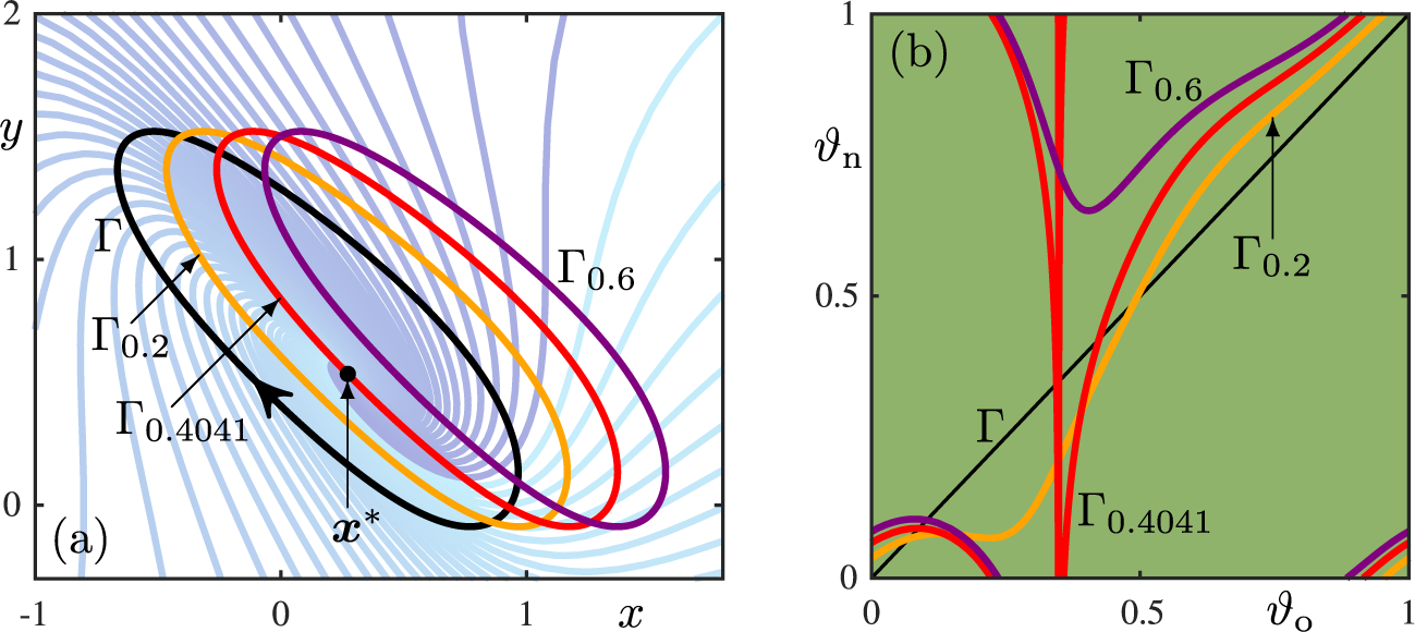
Note that the perturbation set $\Gamma _{0.4041}$
(red curve) in Figure 1(a) passes exactly through the repelling focus
$\Gamma _{0.4041}$
(red curve) in Figure 1(a) passes exactly through the repelling focus $\boldsymbol {x}^*$
around which the isochrons spiral; indeed,
$\boldsymbol {x}^*$
around which the isochrons spiral; indeed, $A = A_c$
is the unique perturbation amplitude with this property, and we refer to it as the critical amplitude
$A = A_c$
is the unique perturbation amplitude with this property, and we refer to it as the critical amplitude $A_c$
. Its relevance is the following. For the perturbation amplitude
$A_c$
. Its relevance is the following. For the perturbation amplitude $A = 0.2$
well before
$A = 0.2$
well before $A_c$
, the perturbation set
$A_c$
, the perturbation set $\Gamma _A$
crosses all isochrons, meaning that the PTC covers the full range of
$\Gamma _A$
crosses all isochrons, meaning that the PTC covers the full range of $\vartheta _{\mathrm {n}} \in [0,1)$
. Figure 1(b) shows that the PTC for
$\vartheta _{\mathrm {n}} \in [0,1)$
. Figure 1(b) shows that the PTC for $A = 0.2$
(orange curve) can be viewed as a smooth deformation of the diagonal, which corresponds to a phase reset with
$A = 0.2$
(orange curve) can be viewed as a smooth deformation of the diagonal, which corresponds to a phase reset with $A = 0$
, that is, to
$A = 0$
, that is, to $\Gamma $
itself. Note that the PTC for
$\Gamma $
itself. Note that the PTC for $A = 0.2$
is a continuous smooth curve on the torus
$A = 0.2$
is a continuous smooth curve on the torus $\mathbb {S}^1 \times \mathbb {S}^1$
, represented by the fundamental square
$\mathbb {S}^1 \times \mathbb {S}^1$
, represented by the fundamental square $[0, 1] \times [0, 1]$
. Similarly, when
$[0, 1] \times [0, 1]$
. Similarly, when $A = 0.6$
past
$A = 0.6$
past $A_c$
, the perturbation set
$A_c$
, the perturbation set $\Gamma _A$
crosses only a subset of the isochron family. The resulting PTC (purple curve) in Figure 1(b) is again a smooth curve on the torus, but it is now topologically different. Indeed, for
$\Gamma _A$
crosses only a subset of the isochron family. The resulting PTC (purple curve) in Figure 1(b) is again a smooth curve on the torus, but it is now topologically different. Indeed, for $0 \leq A < A_c$
, the PTC is a
$0 \leq A < A_c$
, the PTC is a $1\! : \!1$
torus knot, while for
$1\! : \!1$
torus knot, while for $A> A_c$
, it is a
$A> A_c$
, it is a $1\! : \!0$
torus knot [Reference Langfield, Krauskopf, Osinga, Junge, Schütze, Froyland, Ober-Blöbaum and Padberg-Gehle13, Reference Pérez-Cervera, Seara and Huguet17]; Winfree called such resets Type-1 and Type-0 resets, respectively [Reference Winfree22].
$1\! : \!0$
torus knot [Reference Langfield, Krauskopf, Osinga, Junge, Schütze, Froyland, Ober-Blöbaum and Padberg-Gehle13, Reference Pérez-Cervera, Seara and Huguet17]; Winfree called such resets Type-1 and Type-0 resets, respectively [Reference Winfree22].
Precisely at $A = A_c$
, the PTC is singular: the point on
$A = A_c$
, the PTC is singular: the point on $\Gamma $
with phase
$\Gamma $
with phase $\vartheta _{\mathrm {o}} \approx 0.3484$
resets to
$\vartheta _{\mathrm {o}} \approx 0.3484$
resets to $\boldsymbol {x}^*$
. In Figure 1(b), the new phase
$\boldsymbol {x}^*$
. In Figure 1(b), the new phase $\vartheta _{\mathrm {n}}$
approaches negative infinity in the covering space
$\vartheta _{\mathrm {n}}$
approaches negative infinity in the covering space $\mathbb {R}$
of
$\mathbb {R}$
of $\vartheta _{\mathrm {n}}$
as this value of
$\vartheta _{\mathrm {n}}$
as this value of $\vartheta _{\mathrm {o}}$
is approached from either side. Winfree referred to such an event as oscillator death [Reference Winfree21] and he realized that it separates the above topologically different cases of PTCs; see also [Reference Best1, Reference Glass and Winfree6]. Remarkably, Winfree was able to construct an idealized sketch of a surface in
$\vartheta _{\mathrm {o}}$
is approached from either side. Winfree referred to such an event as oscillator death [Reference Winfree21] and he realized that it separates the above topologically different cases of PTCs; see also [Reference Best1, Reference Glass and Winfree6]. Remarkably, Winfree was able to construct an idealized sketch of a surface in $(\vartheta _{\mathrm {o}}, A, \vartheta _{\mathrm {n}})$
-space [Reference Winfree, Urquhart and Yates19, Figure 5], based on approximately 300 experimental data points resulting from phase reset experiments (on yeast cells) at varying phases
$(\vartheta _{\mathrm {o}}, A, \vartheta _{\mathrm {n}})$
-space [Reference Winfree, Urquhart and Yates19, Figure 5], based on approximately 300 experimental data points resulting from phase reset experiments (on yeast cells) at varying phases $\vartheta _{\mathrm {o}}$
and perturbation amplitudes A. He observed that his sketch resembles a “spiral staircase rising counterclockwise” and explained that the rotation axis points to an isolated singular stimulus in the
$\vartheta _{\mathrm {o}}$
and perturbation amplitudes A. He observed that his sketch resembles a “spiral staircase rising counterclockwise” and explained that the rotation axis points to an isolated singular stimulus in the $(\vartheta _{\mathrm {o}}, A)$
-plane; the singular stimulus is precisely the perturbation with amplitude
$(\vartheta _{\mathrm {o}}, A)$
-plane; the singular stimulus is precisely the perturbation with amplitude $A = A_c$
that leads to an interaction with
$A = A_c$
that leads to an interaction with $\boldsymbol {x}^*$
. More precisely, Winfree’s surface is a helix with its axis the vertical line through the point
$\boldsymbol {x}^*$
. More precisely, Winfree’s surface is a helix with its axis the vertical line through the point $(\vartheta _{\mathrm {o}}, A)$
with
$(\vartheta _{\mathrm {o}}, A)$
with $A = A_c$
and
$A = A_c$
and $\vartheta _{\mathrm {o}}$
the phase of the point on
$\vartheta _{\mathrm {o}}$
the phase of the point on $\Gamma $
that resets to
$\Gamma $
that resets to $\boldsymbol {x}^*$
for this critical perturbation amplitude. Mathematically speaking, Winfree’s spiralling staircase is a ruled surface, which requires that all isochrons are straight rays and hence, do not spiral around the phaseless point. However, this is not the typical situation for resets interacting with a single phaseless point, because it requires that the period of the periodic orbit is exactly the time it takes to complete a (small) rotation around the singularity. We suspect that the expansion rate near the phaseless point (relative to the difference in rotation speed) was so strong in Winfree’s experiment that the spiralling behaviour was very minimal and could not be resolved in his experiment.
$\boldsymbol {x}^*$
for this critical perturbation amplitude. Mathematically speaking, Winfree’s spiralling staircase is a ruled surface, which requires that all isochrons are straight rays and hence, do not spiral around the phaseless point. However, this is not the typical situation for resets interacting with a single phaseless point, because it requires that the period of the periodic orbit is exactly the time it takes to complete a (small) rotation around the singularity. We suspect that the expansion rate near the phaseless point (relative to the difference in rotation speed) was so strong in Winfree’s experiment that the spiralling behaviour was very minimal and could not be resolved in his experiment.
In this paper, we present the FitzHugh–Nagumo system as the typical case of phase resetting in a planar system with a phaseless point. Specifically, the requirement is that the isochrons spiral around this point because there is (generically) a difference between the period of $\Gamma $
and the rotational speed around the phaseless point. We explained this in a previous work [Reference Lee, Broderick, Krauskopf and Osinga14], where we studied a family of planar model vector fields, also due to Winfree, for which the isochrons are known explicitly. However, that example has rotational symmetry and, hence, is highly nongeneric. More generally, studies to date of changes in the PTC for varying perturbation amplitudes focused on similar simplified examples [Reference Ermentrout, Glass and Oldeman3, Reference Ermentrout and Terman4, Reference Langfield, Krauskopf and Osinga12, Reference Lee, Broderick, Krauskopf and Osinga14, Reference Winfree20] that exhibit symmetries to aid in the analysis, or on very realistic models [Reference Best1, Reference Glass and Winfree6, Reference Langfield, Krauskopf, Osinga, Junge, Schütze, Froyland, Ober-Blöbaum and Padberg-Gehle13, Reference Osinga and Moehlis16–Reference Schultheiss, Prinz and Butera18] with a complexity that obscures the essential underlying mechanisms. In contrast, the FitzHugh–Nagumo system has no symmetries and the difference in rotation speeds around
$\Gamma $
and the rotational speed around the phaseless point. We explained this in a previous work [Reference Lee, Broderick, Krauskopf and Osinga14], where we studied a family of planar model vector fields, also due to Winfree, for which the isochrons are known explicitly. However, that example has rotational symmetry and, hence, is highly nongeneric. More generally, studies to date of changes in the PTC for varying perturbation amplitudes focused on similar simplified examples [Reference Ermentrout, Glass and Oldeman3, Reference Ermentrout and Terman4, Reference Langfield, Krauskopf and Osinga12, Reference Lee, Broderick, Krauskopf and Osinga14, Reference Winfree20] that exhibit symmetries to aid in the analysis, or on very realistic models [Reference Best1, Reference Glass and Winfree6, Reference Langfield, Krauskopf, Osinga, Junge, Schütze, Froyland, Ober-Blöbaum and Padberg-Gehle13, Reference Osinga and Moehlis16–Reference Schultheiss, Prinz and Butera18] with a complexity that obscures the essential underlying mechanisms. In contrast, the FitzHugh–Nagumo system has no symmetries and the difference in rotation speeds around $\Gamma $
and
$\Gamma $
and $\boldsymbol {x}^*$
is sufficiently large to observe the details of the generic changes of the PTC, as the perturbation amplitude A is increased through
$\boldsymbol {x}^*$
is sufficiently large to observe the details of the generic changes of the PTC, as the perturbation amplitude A is increased through $A_c$
. This is in contrast to the example of the Van der Pol system that was also studied in [Reference Lee, Broderick, Krauskopf and Osinga14], but for which the difference in rotation speed turned out to be too small—much like what we suspect was the case in Winfree’s experiment [Reference Winfree, Urquhart and Yates19]. Moreover, the Van der Pol system still has a symmetry; namely, it is invariant under rotation by
$A_c$
. This is in contrast to the example of the Van der Pol system that was also studied in [Reference Lee, Broderick, Krauskopf and Osinga14], but for which the difference in rotation speed turned out to be too small—much like what we suspect was the case in Winfree’s experiment [Reference Winfree, Urquhart and Yates19]. Moreover, the Van der Pol system still has a symmetry; namely, it is invariant under rotation by $\pi $
around the origin, which is the phaseless point.
$\pi $
around the origin, which is the phaseless point.
In this paper, we show that as A increases through $A_c$
, there is an infinite sequence of twin tangencies, where the phase reset is such that the shifted periodic orbit
$A_c$
, there is an infinite sequence of twin tangencies, where the phase reset is such that the shifted periodic orbit $\Gamma $
has two separate points of tangency with one and the same isochron. Each such twin tangency changes how many times the unit interval of
$\Gamma $
has two separate points of tangency with one and the same isochron. Each such twin tangency changes how many times the unit interval of $\vartheta _{\mathrm {n}}$
is covered by the PTC, which increases to infinity as
$\vartheta _{\mathrm {n}}$
is covered by the PTC, which increases to infinity as $A \nearrow A_c$
and then decreases again past
$A \nearrow A_c$
and then decreases again past $A=A_c$
. We are able to identify and illustrate clearly such twin tangencies of the FitzHugh–Nagumo system, which is a representative for a generic planar vector field. Moreover, we discuss how these changes of the PTC (for a given direction of perturbation) are encoded by the geometry of the phase-resetting surface in
$A=A_c$
. We are able to identify and illustrate clearly such twin tangencies of the FitzHugh–Nagumo system, which is a representative for a generic planar vector field. Moreover, we discuss how these changes of the PTC (for a given direction of perturbation) are encoded by the geometry of the phase-resetting surface in $(\vartheta _{\mathrm {o}}, A, \vartheta _{\mathrm {n}})$
-space. Colloquially speaking, owing to the spiralling nature of the isochrons near
$(\vartheta _{\mathrm {o}}, A, \vartheta _{\mathrm {n}})$
-space. Colloquially speaking, owing to the spiralling nature of the isochrons near $\vartheta _{\mathrm {n}}$
, this surface rolls up around a singular vertical line at
$\vartheta _{\mathrm {n}}$
, this surface rolls up around a singular vertical line at $A=A_c$
and the corresponding value of
$A=A_c$
and the corresponding value of $\vartheta _{\mathrm {o}}$
, and this has the observed consequences for the transition of the PTC. We also present a discussion of phase resets with perturbations in different directions (given by an angle
$\vartheta _{\mathrm {o}}$
, and this has the observed consequences for the transition of the PTC. We also present a discussion of phase resets with perturbations in different directions (given by an angle $\varphi _{\mathrm {d}}$
), which are associated with different values of
$\varphi _{\mathrm {d}}$
), which are associated with different values of $A_c$
and
$A_c$
and $\vartheta _{\mathrm {o}}$
. To this end, we present the phase-resetting surface in
$\vartheta _{\mathrm {o}}$
. To this end, we present the phase-resetting surface in $(\vartheta _{\mathrm {o}}, \varphi _{\mathrm {d}}, \vartheta _{\mathrm {n}})$
-space and show how it changes with the perturbation amplitude A. To obtain these results, we compute isochrons and PTCs with a boundary-value problem setup that was implemented within the package COCO [Reference Dankowicz and Schilder2] (see [Reference Hannam, Krauskopf and Osinga9, Reference Langfield, Krauskopf, Osinga, Junge, Schütze, Froyland, Ober-Blöbaum and Padberg-Gehle13, Reference Osinga and Moehlis16] for more details).
$(\vartheta _{\mathrm {o}}, \varphi _{\mathrm {d}}, \vartheta _{\mathrm {n}})$
-space and show how it changes with the perturbation amplitude A. To obtain these results, we compute isochrons and PTCs with a boundary-value problem setup that was implemented within the package COCO [Reference Dankowicz and Schilder2] (see [Reference Hannam, Krauskopf and Osinga9, Reference Langfield, Krauskopf, Osinga, Junge, Schütze, Froyland, Ober-Blöbaum and Padberg-Gehle13, Reference Osinga and Moehlis16] for more details).
This paper is organized as follows. In Section 2, we introduce the FitzHugh–Nagumo system and state the specific parameter values we use. Section 3 then introduces its PTC for a perturbation in the positive x-direction and how the PTC is defined as the graph of a function that depends on the perturbation amplitude A. This includes a discussion of the loss of invertibility of this function in Section 3.1 and its changes due to twin tangencies in Section 3.2; the associated phase-resetting surface in $(\vartheta _{\mathrm {o}}, A, \vartheta _{\mathrm {n}})$
-space is introduced and presented in Section 3.3. In Section 4, we discuss the influence of the direction of the perturbation, as represented by the angle
$(\vartheta _{\mathrm {o}}, A, \vartheta _{\mathrm {n}})$
-space is introduced and presented in Section 3.3. In Section 4, we discuss the influence of the direction of the perturbation, as represented by the angle $\varphi _{\mathrm {d}}$
; the five qualitatively different cases of the phase-resetting surface for fixed A are presented and discussed in Section 4.1. We present in Section 5 a discussion and brief outlook on possible future work, and include a short presentation of the computational setup in Appendix A.
$\varphi _{\mathrm {d}}$
; the five qualitatively different cases of the phase-resetting surface for fixed A are presented and discussed in Section 4.1. We present in Section 5 a discussion and brief outlook on possible future work, and include a short presentation of the computational setup in Appendix A.
2 The FitzHugh–Nagumo system
Winfree [Reference Winfree22] studied the FitzHugh–Nagumo system [Reference FitzHugh5, Reference Nagumo, Arimoto and Yoshizawa15] as a typical planar example that cannot be analysed explicitly. He wrote the system as
 $$ \begin{align} \begin{cases} \dot{x} = c \bigg(y + x - \dfrac{1}{3} \, x^3 + z\bigg), \\[4pt] \dot{y} = -\dfrac{1}{c} (x - a + b \, y), \end{cases} \end{align} $$
and his interest was in the regime for which this system has an attracting periodic orbit $\Gamma $
with a repelling focus equilibrium
$\Gamma $
with a repelling focus equilibrium $\boldsymbol {x}^*$
as the single phaseless point. His numerical explorations suggested that the isochron structure is extremely complicated, which was later confirmed with more advanced computational methods [Reference Langfield, Krauskopf and Osinga11]. An immediate consequence of such a complex isochron structure is that the FitzHugh–Nagumo system may feature complicated PTCs for phase resets well before the interaction with the phaseless point [Reference Langfield, Krauskopf, Osinga, Junge, Schütze, Froyland, Ober-Blöbaum and Padberg-Gehle13]. One particular reason for this complexity is a significant difference in time scales between the evolutions of the x- and y-coordinates, as given by the choice for the parameter c [Reference Langfield, Krauskopf and Osinga12].
$\boldsymbol {x}^*$
as the single phaseless point. His numerical explorations suggested that the isochron structure is extremely complicated, which was later confirmed with more advanced computational methods [Reference Langfield, Krauskopf and Osinga11]. An immediate consequence of such a complex isochron structure is that the FitzHugh–Nagumo system may feature complicated PTCs for phase resets well before the interaction with the phaseless point [Reference Langfield, Krauskopf, Osinga, Junge, Schütze, Froyland, Ober-Blöbaum and Padberg-Gehle13]. One particular reason for this complexity is a significant difference in time scales between the evolutions of the x- and y-coordinates, as given by the choice for the parameter c [Reference Langfield, Krauskopf and Osinga12].
We consider system (2.1) in the same parameter regime as Winfree, but set $c = 1$
, so that there is effectively no time-scale separation; moreover, we introduce the off-set
$c = 1$
, so that there is effectively no time-scale separation; moreover, we introduce the off-set $z = -0.8$
to move the equilibrium away from the origin. This choice of parameter values is given in Table 1 and it results in the overall structure of isochrons of the FitzHugh–Nagumo system as illustrated in Figure 1(a). More specifically, the attracting periodic orbit
$z = -0.8$
to move the equilibrium away from the origin. This choice of parameter values is given in Table 1 and it results in the overall structure of isochrons of the FitzHugh–Nagumo system as illustrated in Figure 1(a). More specifically, the attracting periodic orbit $\Gamma $
of system (2.1) has
$\Gamma $
of system (2.1) has $T_\Gamma \approx 10.8329$
and it surrounds the repelling focus
$T_\Gamma \approx 10.8329$
and it surrounds the repelling focus $\boldsymbol {x}^* \approx (0.2729, 0.5339)$
with eigenvalues
$\boldsymbol {x}^* \approx (0.2729, 0.5339)$
with eigenvalues $0.0628 \pm 0.5056 \, i$
, which constitutes the only point in the phaseless set. As is the convention in the field, we define the zero-phase point
$0.0628 \pm 0.5056 \, i$
, which constitutes the only point in the phaseless set. As is the convention in the field, we define the zero-phase point $\gamma _0 \approx (0.9660, 0.1345) \in \Gamma $
as the point with the maximum value of the x-coordinate. Since the motion along
$\gamma _0 \approx (0.9660, 0.1345) \in \Gamma $
as the point with the maximum value of the x-coordinate. Since the motion along $\Gamma $
is clockwise and the rotation period around
$\Gamma $
is clockwise and the rotation period around $\boldsymbol {x}^*$
is larger than
$\boldsymbol {x}^*$
is larger than $T_\Gamma $
, the isochrons of
$T_\Gamma $
, the isochrons of $\Gamma $
spiral around
$\Gamma $
spiral around $\boldsymbol {x}^*$
in the clockwise direction [see Figure 1(a)].
$\boldsymbol {x}^*$
in the clockwise direction [see Figure 1(a)].
The values of the parameters of the FitzHugh–Nagumo system (2.1) that are used throughout.
3 PTCs for varying perturbation amplitude
The three PTCs illustrated in Figure 1 for the FitzHugh–Nagumo system (2.1) with parameters as in Table 1 are only part of the story of the transition from a $1\! : \!1$
to a
$1\! : \!1$
to a $1\! : \!0$
torus knot. As the perturbation amplitude A increases towards
$1\! : \!0$
torus knot. As the perturbation amplitude A increases towards $A_c$
, the PTC changes dramatically. To aid the discussion, we define the phase-resetting function
$A_c$
, the PTC changes dramatically. To aid the discussion, we define the phase-resetting function
 $$ \begin{align} \mathcal{P}_A: \vartheta_{\mathrm{o}} \in [0,1) \to \vartheta_{\mathrm{n}} \in [0,1) \end{align} $$
as the function from the old to the new phase, which has the PTC with given perturbation amplitude $A \geq 0$
as its graph, denoted as
$A \geq 0$
as its graph, denoted as $\mathrm {graph}(\mathcal {P}_A)$
. Throughout this section, we consider exclusively perturbations in the fixed direction of increasing x, in the form of an instantaneous reset that translates the x-coordinate to the value at distance A in the positive direction, as was done in Figure 1. The phase-resetting function
$\mathrm {graph}(\mathcal {P}_A)$
. Throughout this section, we consider exclusively perturbations in the fixed direction of increasing x, in the form of an instantaneous reset that translates the x-coordinate to the value at distance A in the positive direction, as was done in Figure 1. The phase-resetting function $\mathcal {P}_0$
(in the absence of a perturbation) is the identity, meaning that the PTC for
$\mathcal {P}_0$
(in the absence of a perturbation) is the identity, meaning that the PTC for $A = 0$
is the diagonal, labelled
$A = 0$
is the diagonal, labelled $\Gamma $
in Figure 1(b) and similar figures. In particular, this means that
$\Gamma $
in Figure 1(b) and similar figures. In particular, this means that $\mathcal {P}_A$
is invertible when A is sufficiently small. However, when A becomes too large, invertibility of
$\mathcal {P}_A$
is invertible when A is sufficiently small. However, when A becomes too large, invertibility of $\mathcal {P}_A$
is lost.
$\mathcal {P}_A$
is lost.
3.1 Loss of invertibility
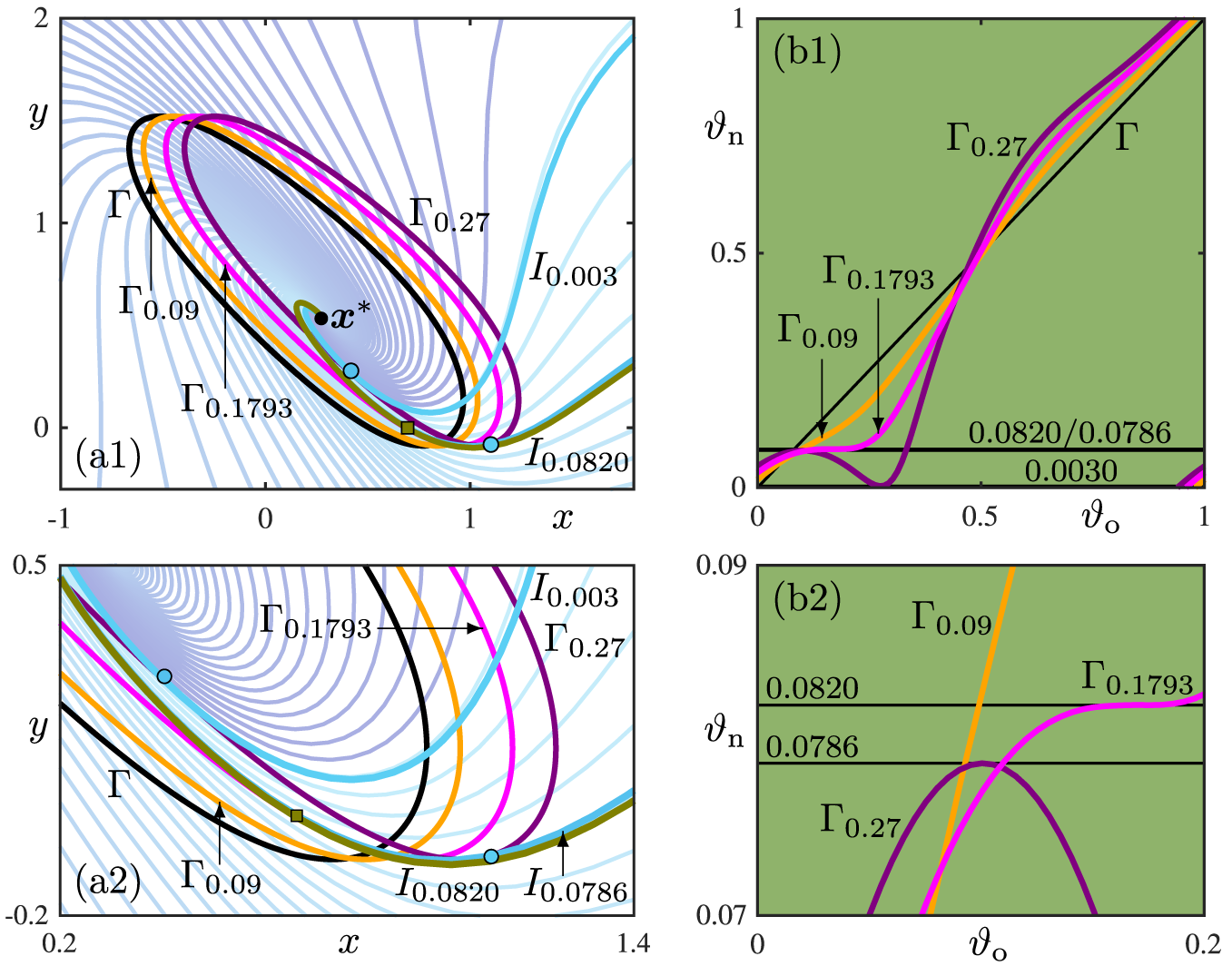
Figure 2 illustrates the loss of invertibility in the style of Figure 1 with the perturbation sets and PTCs for $A = 0.09$
(orange curves),
$A = 0.09$
(orange curves), $A = 0.1793$
(magenta curves) and
$A = 0.1793$
(magenta curves) and $A = 0.27$
(purple curves). Panels (a1) and (a2) of Figure 2 show
$A = 0.27$
(purple curves). Panels (a1) and (a2) of Figure 2 show $\Gamma $
with the three shifted perturbation sets together with three highlighted isochrons, and panels (b1) and (b2) show the corresponding PTCs. The perturbation set
$\Gamma $
with the three shifted perturbation sets together with three highlighted isochrons, and panels (b1) and (b2) show the corresponding PTCs. The perturbation set $\Gamma _A$
for
$\Gamma _A$
for $A = 0.09$
(orange curve) intersects all isochrons transversely and, consequently,
$A = 0.09$
(orange curve) intersects all isochrons transversely and, consequently, $\mathcal {P}_A$
is invertible and the PTC is monotonically increasing. At
$\mathcal {P}_A$
is invertible and the PTC is monotonically increasing. At $A \approx 0.1793$
, the perturbation set (magenta curve) has a cubic tangency with the isochron
$A \approx 0.1793$
, the perturbation set (magenta curve) has a cubic tangency with the isochron $I_{0.0820}$
, which means that the PTC has an inflection point at the value
$I_{0.0820}$
, which means that the PTC has an inflection point at the value $\vartheta _{\mathrm {n}} = 0.0820$
; see the enlargement panels (a2) and (b2). For larger values of A, the perturbation set
$\vartheta _{\mathrm {n}} = 0.0820$
; see the enlargement panels (a2) and (b2). For larger values of A, the perturbation set $\Gamma _A$
has quadratic tangencies with two different isochrons; for the case
$\Gamma _A$
has quadratic tangencies with two different isochrons; for the case $A = 0.27$
(purple curves) shown in Figure 2, these are
$A = 0.27$
(purple curves) shown in Figure 2, these are $I_{0.0786}$
and
$I_{0.0786}$
and $I_{0.0030}$
. As a consequence, the PTC is no longer invertible: for
$I_{0.0030}$
. As a consequence, the PTC is no longer invertible: for $A = 0.27$
, it has a local maximum at
$A = 0.27$
, it has a local maximum at $\vartheta _{\mathrm {n}} = 0.0786$
and a local minimum at
$\vartheta _{\mathrm {n}} = 0.0786$
and a local minimum at $\vartheta _{\mathrm {n}} = 0.0030$
. Indeed, Figure 2 clearly illustrates that the loss of invertibility of the PTC is due to the cubic tangency of the perturbation set with an isochron; see also [Reference Langfield, Krauskopf, Osinga, Junge, Schütze, Froyland, Ober-Blöbaum and Padberg-Gehle13, Reference Pérez-Cervera, Seara and Huguet17].
$\vartheta _{\mathrm {n}} = 0.0030$
. Indeed, Figure 2 clearly illustrates that the loss of invertibility of the PTC is due to the cubic tangency of the perturbation set with an isochron; see also [Reference Langfield, Krauskopf, Osinga, Junge, Schütze, Froyland, Ober-Blöbaum and Padberg-Gehle13, Reference Pérez-Cervera, Seara and Huguet17].
Transition through the cubic tangency at $A \approx 0.1793$
. Panel (a1) shows
$A \approx 0.1793$
. Panel (a1) shows $\Gamma $
(black),
$\Gamma $
(black), $\Gamma _{0.09}$
(orange),
$\Gamma _{0.09}$
(orange), $\Gamma _{0.1793}$
(magenta) and
$\Gamma _{0.1793}$
(magenta) and $\Gamma _{0.27}$
(purple), with the isochrons
$\Gamma _{0.27}$
(purple), with the isochrons $I_{0.0820}$
(olive),
$I_{0.0820}$
(olive), $I_{0.0786}$
and
$I_{0.0786}$
and $I_{0.0030}$
(both light blue); panel (b1) shows the corresponding three PTCs in matching colours in the fundamental square, where the
$I_{0.0030}$
(both light blue); panel (b1) shows the corresponding three PTCs in matching colours in the fundamental square, where the $\vartheta _{\mathrm {n}}$
-values of tangencies are shown as horizontal lines. Panels (a2) and (b2) are respective enlargements near the cubic tangency.
$\vartheta _{\mathrm {n}}$
-values of tangencies are shown as horizontal lines. Panels (a2) and (b2) are respective enlargements near the cubic tangency.
The first twin tangency at $A \approx 0.4032 < A_c$
. Panel (a1) shows
$A \approx 0.4032 < A_c$
. Panel (a1) shows $\Gamma $
(black) with
$\Gamma $
(black) with $\Gamma _{0.4032}$
(magenta) and the isochron
$\Gamma _{0.4032}$
(magenta) and the isochron $I_{0.0881}$
(olive); and panel (a2) with its inset show successive enlargements near the twin tangency points. The corresponding PTC is shown in panel (b) in the fundamental square (green shading) and as a single smooth curve over the extended
$I_{0.0881}$
(olive); and panel (a2) with its inset show successive enlargements near the twin tangency points. The corresponding PTC is shown in panel (b) in the fundamental square (green shading) and as a single smooth curve over the extended $\vartheta _{\mathrm {n}}$
-range of
$\vartheta _{\mathrm {n}}$
-range of $[-1, 1]$
.
$[-1, 1]$
.
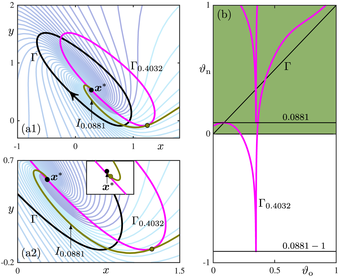
3.2 First and last twin tangency
As A is increased further towards $A_c$
, the local maximum of the PTC moves up in
$A_c$
, the local maximum of the PTC moves up in $\vartheta _{\mathrm {n}}$
and its local minimum moves down. Since
$\vartheta _{\mathrm {n}}$
and its local minimum moves down. Since $\vartheta _{\mathrm {n}}$
is taken modulo
$\vartheta _{\mathrm {n}}$
is taken modulo $1$
on the fundamental square, the local maximum and minimum eventually have equal values, which marks a transition in terms of how many times the full range of
$1$
on the fundamental square, the local maximum and minimum eventually have equal values, which marks a transition in terms of how many times the full range of $\vartheta _{\mathrm {n}} \in [0, 1)$
is covered by
$\vartheta _{\mathrm {n}} \in [0, 1)$
is covered by $\mathcal {P}_A$
and, hence, the PTC. Geometrically, when viewed in the phase plane, this means that the perturbation set has (quadratic) tangencies with two isochrons that lie increasingly further apart in the family, until their phase difference reaches
$\mathcal {P}_A$
and, hence, the PTC. Geometrically, when viewed in the phase plane, this means that the perturbation set has (quadratic) tangencies with two isochrons that lie increasingly further apart in the family, until their phase difference reaches $0.5$
; these two isochrons at which the tangencies occur then come closer together and eventually become one and the same isochron. We call this a twin tangency and Figure 3 illustrates the first one as A is increased, which occurs at
$0.5$
; these two isochrons at which the tangencies occur then come closer together and eventually become one and the same isochron. We call this a twin tangency and Figure 3 illustrates the first one as A is increased, which occurs at $A \approx 0.4032$
. Panel (a1) shows that
$A \approx 0.4032$
. Panel (a1) shows that $\Gamma _{0.4032}$
(magenta) is tangent to the single isochron
$\Gamma _{0.4032}$
(magenta) is tangent to the single isochron $I_{0.0881}$
(olive) at two different points; note from the enlargements in panel (a2) that one of these tangencies is very close to the phaseless point
$I_{0.0881}$
(olive) at two different points; note from the enlargements in panel (a2) that one of these tangencies is very close to the phaseless point $\boldsymbol {x}^*$
. The representation in Figure 3(b) of the PTC over the extended
$\boldsymbol {x}^*$
. The representation in Figure 3(b) of the PTC over the extended $\vartheta _{\mathrm {n}}$
-range
$\vartheta _{\mathrm {n}}$
-range $[-1,1]$
illustrates that its maximum and minimum have a difference of
$[-1,1]$
illustrates that its maximum and minimum have a difference of $1$
in the covering space and, hence, have the same
$1$
in the covering space and, hence, have the same $\vartheta _{\mathrm {n}}$
-value in the fundamental square. Notice that
$\vartheta _{\mathrm {n}}$
-value in the fundamental square. Notice that $\Gamma _{0.4032}$
intersects every isochron precisely three times; equivalently, the PTC in Figure 3(b) covers the
$\Gamma _{0.4032}$
intersects every isochron precisely three times; equivalently, the PTC in Figure 3(b) covers the $\vartheta _{\mathrm {n}}$
-range
$\vartheta _{\mathrm {n}}$
-range $[0, 1)$
of the torus precisely three times. The PTC remains a
$[0, 1)$
of the torus precisely three times. The PTC remains a $1\! : \!1$
torus knot, because the overall increase of
$1\! : \!1$
torus knot, because the overall increase of $\vartheta_{\mathrm{n}}$
with
$\vartheta_{\mathrm{n}}$
with $\vartheta_{\mathrm{o}} \in [0, 1)$
is still
$\vartheta_{\mathrm{o}} \in [0, 1)$
is still $1$
.
$1$
.
The last twin tangency at $A \approx 0.4168> A_c$
. Panel (a1) shows
$A \approx 0.4168> A_c$
. Panel (a1) shows $\Gamma $
(black) with
$\Gamma $
(black) with $\Gamma _{0.4168}$
(cyan) and the isochron
$\Gamma _{0.4168}$
(cyan) and the isochron $I_{0.0892}$
(olive); and panel (a2) and its inset are successive enlargements near the twin tangency points. The corresponding PTC is shown in panel (b) in the fundamental square (green shading) and as a single smooth curve over the extended
$I_{0.0892}$
(olive); and panel (a2) and its inset are successive enlargements near the twin tangency points. The corresponding PTC is shown in panel (b) in the fundamental square (green shading) and as a single smooth curve over the extended $\vartheta _{\mathrm {n}}$
-range of
$\vartheta _{\mathrm {n}}$
-range of $[-1, 1]$
.
$[-1, 1]$
.

As Winfree already pointed out [Reference Winfree, Urquhart and Yates19, Reference Winfree22], the PTC changes topological type from a $1\! : \!1$
torus knot (Type-1 reset) to a
$1\! : \!1$
torus knot (Type-1 reset) to a $1\! : \!0$
torus knot (Type-0 reset) when A is increased through
$1\! : \!0$
torus knot (Type-0 reset) when A is increased through $A = A_c$
. For the general case where the isochrons spiral around the phaseless point, as is the case here, the PTC covers the unit
$A = A_c$
. For the general case where the isochrons spiral around the phaseless point, as is the case here, the PTC covers the unit $\vartheta _{\mathrm {n}}$
-interval of the fundamental square ever more as A is increased further towards
$\vartheta _{\mathrm {n}}$
-interval of the fundamental square ever more as A is increased further towards $A_c$
[Reference Lee, Broderick, Krauskopf and Osinga14]. Specifically for system (2.1), the minimum of the PTC moves towards increasingly lower values of
$A_c$
[Reference Lee, Broderick, Krauskopf and Osinga14]. Specifically for system (2.1), the minimum of the PTC moves towards increasingly lower values of $\vartheta _{\mathrm {n}}$
, such that there is an infinite sequence of twin tangencies, each increasing the number of coverings of the unit interval by
$\vartheta _{\mathrm {n}}$
, such that there is an infinite sequence of twin tangencies, each increasing the number of coverings of the unit interval by $2$
. For
$2$
. For $A = A_c$
, the unit
$A = A_c$
, the unit $\vartheta _{\mathrm {n}}$
-interval is covered infinitely many times, and for A past the critical value
$\vartheta _{\mathrm {n}}$
-interval is covered infinitely many times, and for A past the critical value $A_c$
, there is a sequence of twin tangencies in reverse that reduces the number of times the
$A_c$
, there is a sequence of twin tangencies in reverse that reduces the number of times the $\vartheta _{\mathrm {n}}$
-range
$\vartheta _{\mathrm {n}}$
-range $[0, 1)$
is covered. The difference is that, at each twin tangency for
$[0, 1)$
is covered. The difference is that, at each twin tangency for $A> A_c$
, the perturbation set
$A> A_c$
, the perturbation set $\Gamma _A$
now crosses all isochrons exactly an even number of times. Figure 4 illustrates the last twin tangency of this reverse sequence in the style of Figure 3. As panels (a1) and (a2) of Figure 4 show, the perturbation set
$\Gamma _A$
now crosses all isochrons exactly an even number of times. Figure 4 illustrates the last twin tangency of this reverse sequence in the style of Figure 3. As panels (a1) and (a2) of Figure 4 show, the perturbation set $\Gamma _{0.4168}$
(magenta) has two points of quadratic tangency with one and the same isochron
$\Gamma _{0.4168}$
(magenta) has two points of quadratic tangency with one and the same isochron $I_{0.0892}$
(olive). Note that, compared with the first twin tangency, the perturbation set and the second tangency point is now “on the other side” of the phaseless point
$I_{0.0892}$
(olive). Note that, compared with the first twin tangency, the perturbation set and the second tangency point is now “on the other side” of the phaseless point $\boldsymbol {x}^*$
. The PTC in Figure 4(b) is now a
$\boldsymbol {x}^*$
. The PTC in Figure 4(b) is now a $1\! : \!0$
torus knot that covers
$1\! : \!0$
torus knot that covers $[0, 1)$
exactly twice. After this last twin tangency, for
$[0, 1)$
exactly twice. After this last twin tangency, for $A> 0.4168$
, the PTC loses surjectivity and no longer covers the full range of
$A> 0.4168$
, the PTC loses surjectivity and no longer covers the full range of $\vartheta _{\mathrm {n}}$
: the transition through
$\vartheta _{\mathrm {n}}$
: the transition through $A_c$
is complete (see the case for
$A_c$
is complete (see the case for $A = 0.6$
in Figure 1(b)).
$A = 0.6$
in Figure 1(b)).
3.3 Phase-resetting surface near its singularity
The entire transition of the PTC through $A_c$
can be represented geometrically by the phase-resetting surface consisting of the PTCs for any A. More formally, we now consider the function
$A_c$
can be represented geometrically by the phase-resetting surface consisting of the PTCs for any A. More formally, we now consider the function $\mathcal {P}(\vartheta _{\mathrm { o}}, A) := \mathcal {P}_A(\vartheta _{\mathrm {o}})$
over the
$\mathcal {P}(\vartheta _{\mathrm { o}}, A) := \mathcal {P}_A(\vartheta _{\mathrm {o}})$
over the $(\vartheta _{\mathrm {o}}, A)$
-plane, and the phase-resetting surface of system (2.1) in
$(\vartheta _{\mathrm {o}}, A)$
-plane, and the phase-resetting surface of system (2.1) in $(\vartheta _{\mathrm {o}}, A, \vartheta _{\mathrm { n}})$
-space is
$(\vartheta _{\mathrm {o}}, A, \vartheta _{\mathrm { n}})$
-space is $\mathrm {graph}(\mathcal {P}) = \{\mathrm {graph}(\mathcal {P}_A) \mid A \in \mathbb {R}^{\geq 0}\}$
. This surface is shown in Figure 5(a). Specifically, we plot the phase-resetting surface over the extended
$\mathrm {graph}(\mathcal {P}) = \{\mathrm {graph}(\mathcal {P}_A) \mid A \in \mathbb {R}^{\geq 0}\}$
. This surface is shown in Figure 5(a). Specifically, we plot the phase-resetting surface over the extended $\vartheta _{\mathrm {n}}$
-range
$\vartheta _{\mathrm {n}}$
-range $[-1, 2]$
, so that, effectively, three copies or sheets are shown. Our focus here is on a neighbourhood of the singular parameter point S given by
$[-1, 2]$
, so that, effectively, three copies or sheets are shown. Our focus here is on a neighbourhood of the singular parameter point S given by $A = A_c \approx 0.4041$
and
$A = A_c \approx 0.4041$
and $\vartheta _{\mathrm {o}} \approx 0.3484$
, for which the corresponding point on the periodic orbit
$\vartheta _{\mathrm {o}} \approx 0.3484$
, for which the corresponding point on the periodic orbit $\Gamma $
maps exactly to
$\Gamma $
maps exactly to $\boldsymbol {x}^*$
. In
$\boldsymbol {x}^*$
. In $(\vartheta _{\mathrm {o}}, A, \vartheta _{\mathrm {n}})$
-space, this parameter point S gives rise to a singular vertical line, and the phase-resetting surface spirals around it. To aid in its interpretation, Figure 5(a) also shows two lifts each of three PTCs: the PTC for
$(\vartheta _{\mathrm {o}}, A, \vartheta _{\mathrm {n}})$
-space, this parameter point S gives rise to a singular vertical line, and the phase-resetting surface spirals around it. To aid in its interpretation, Figure 5(a) also shows two lifts each of three PTCs: the PTC for $\Gamma _{0.35}$
(orange), which is a
$\Gamma _{0.35}$
(orange), which is a $1\! : \!1$
torus knot; the singular PTC for
$1\! : \!1$
torus knot; the singular PTC for $\Gamma _{0.4041}$
(red) with singularity at S; and the PTC for
$\Gamma _{0.4041}$
(red) with singularity at S; and the PTC for $\Gamma _{0.45}$
(purple), which is a
$\Gamma _{0.45}$
(purple), which is a $1\! : \!0$
torus knot.
$1\! : \!0$
torus knot.
Geometry of the phase-resetting surface of system (2.1). Panel (a) shows $\mathrm{graph}(\mathcal{P})$
in
$\mathrm{graph}(\mathcal{P})$
in $(\vartheta _{\mathrm {o}}, A, \vartheta _{\mathrm {n}})$
-space near its singular vertical line S over the extended
$(\vartheta _{\mathrm {o}}, A, \vartheta _{\mathrm {n}})$
-space near its singular vertical line S over the extended $\vartheta _{\mathrm {n}}$
-range
$\vartheta _{\mathrm {n}}$
-range $[-1, 2]$
; also shown are two lifts each of the PTCs for
$[-1, 2]$
; also shown are two lifts each of the PTCs for $\Gamma _{0.35}$
(orange),
$\Gamma _{0.35}$
(orange), $\Gamma _{0.4041}$
(red) and
$\Gamma _{0.4041}$
(red) and $\Gamma _{0.45}$
(purple). Panel (b) shows, for comparison, the surface swept out by the isochrons in
$\Gamma _{0.45}$
(purple). Panel (b) shows, for comparison, the surface swept out by the isochrons in $(x, y, \vartheta )$
-space near the phaseless set
$(x, y, \vartheta )$
-space near the phaseless set $\boldsymbol {x}^*$
, over the extended
$\boldsymbol {x}^*$
, over the extended $\vartheta $
-range
$\vartheta $
-range $[-1, 2]$
; the 50 computed isochrons from Figure 1(a) are highlighted for
$[-1, 2]$
; the 50 computed isochrons from Figure 1(a) are highlighted for $\vartheta \in [0, 1]$
.
$\vartheta \in [0, 1]$
.
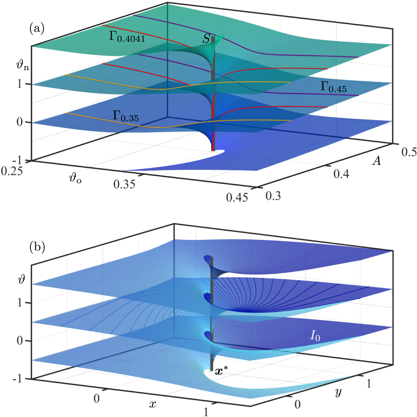
Figure 5(b) shows a very different surface: the one that is swept out by the isochrons when they are shown in $(x, y, \vartheta )$
-space in terms of their
$(x, y, \vartheta )$
-space in terms of their $\vartheta $
-value; here, we also show three copies over the extended
$\vartheta $
-value; here, we also show three copies over the extended $\vartheta $
-range
$\vartheta $
-range $[-1, 2]$
. This isochron surface was generated and rendered from the 50 computed isochrons, which are highlighted on the surface for
$[-1, 2]$
. This isochron surface was generated and rendered from the 50 computed isochrons, which are highlighted on the surface for $\vartheta \in [0,1)$
. The focus is on a region near the phaseless point
$\vartheta \in [0,1)$
. The focus is on a region near the phaseless point $\boldsymbol {x}^*$
, which similarly gives rise to a singular vertical line around which the isochrons spiral. Observe the striking similarity between the phase-resetting surface near S in Figure 5(a) and the isochron surface near
$\boldsymbol {x}^*$
, which similarly gives rise to a singular vertical line around which the isochrons spiral. Observe the striking similarity between the phase-resetting surface near S in Figure 5(a) and the isochron surface near $\boldsymbol {x}^*$
in panel (b). This is explained by the fact that points
$\boldsymbol {x}^*$
in panel (b). This is explained by the fact that points $(\vartheta _{\mathrm {o}}, A)$
near S are mapped smoothly and uniquely to points in the
$(\vartheta _{\mathrm {o}}, A)$
near S are mapped smoothly and uniquely to points in the $(x,y)$
-plane near
$(x,y)$
-plane near $\boldsymbol {x}^*$
by the “action” of the perturbation map, given by
$\boldsymbol {x}^*$
by the “action” of the perturbation map, given by $(\vartheta _{\mathrm {o}}, A) \mapsto \gamma (\vartheta _{\mathrm {o}}) + (A, 0)$
with
$(\vartheta _{\mathrm {o}}, A) \mapsto \gamma (\vartheta _{\mathrm {o}}) + (A, 0)$
with $\gamma (\vartheta _{\mathrm {o}}) \in \Gamma $
. Locally near the singular point S and the phaseless set
$\gamma (\vartheta _{\mathrm {o}}) \in \Gamma $
. Locally near the singular point S and the phaseless set $\boldsymbol {x}^*$
, this perturbation map from the
$\boldsymbol {x}^*$
, this perturbation map from the $(\vartheta _{\mathrm {o}}, A)$
-plane to the
$(\vartheta _{\mathrm {o}}, A)$
-plane to the $(x, y)$
-plane is a bijection [Reference Lee, Broderick, Krauskopf and Osinga14]. Hence, the phase-resetting surface in Figure 5(a) is the diffeomorphic image of the isochron surface in Figure 5(b) under the local inverse of the perturbation map. In particular, it follows that the level set of the phase-resetting surface for any fixed value of
$(x, y)$
-plane is a bijection [Reference Lee, Broderick, Krauskopf and Osinga14]. Hence, the phase-resetting surface in Figure 5(a) is the diffeomorphic image of the isochron surface in Figure 5(b) under the local inverse of the perturbation map. In particular, it follows that the level set of the phase-resetting surface for any fixed value of $\vartheta _{\mathrm {n}}$
is a spiral that accumulates on (but never reaches) the respective point on the vertical line S. In fact, the surface in Figure 5(a) was rendered from a selection of such spirals, each of which was computed as a curve for a fixed value of
$\vartheta _{\mathrm {n}}$
is a spiral that accumulates on (but never reaches) the respective point on the vertical line S. In fact, the surface in Figure 5(a) was rendered from a selection of such spirals, each of which was computed as a curve for a fixed value of $\vartheta _{\mathrm {n}}$
.
$\vartheta _{\mathrm {n}}$
.
The spiralling nature of the phase-resetting surface around the line S in $(\vartheta _{\mathrm {o}}, A, \vartheta _{\mathrm {n}})$
-space is the “geometric encoding” of the fact that the transition of the PTC, as A is increased through
$(\vartheta _{\mathrm {o}}, A, \vartheta _{\mathrm {n}})$
-space is the “geometric encoding” of the fact that the transition of the PTC, as A is increased through $A_c$
, necessarily involves infinite sequences of twin tangencies, as was discussed in Section 3.2. In turn, this is a direct consequence of the spiralling of the isochrons around
$A_c$
, necessarily involves infinite sequences of twin tangencies, as was discussed in Section 3.2. In turn, this is a direct consequence of the spiralling of the isochrons around $\boldsymbol {x}^*$
in the
$\boldsymbol {x}^*$
in the $(x,y)$
-plane. The illustration of this insight in Figure 5 for the FitzHugh–Nagumo system represents the generic case of a planar vector field; a similar illustration is shown in [Reference Lee, Broderick, Krauskopf and Osinga14, Figure 8] for a constructed example due to Winfree with rotational symmetry and analytically known isochrons.
$(x,y)$
-plane. The illustration of this insight in Figure 5 for the FitzHugh–Nagumo system represents the generic case of a planar vector field; a similar illustration is shown in [Reference Lee, Broderick, Krauskopf and Osinga14, Figure 8] for a constructed example due to Winfree with rotational symmetry and analytically known isochrons.
4 Varying the direction of perturbation
The application context of the FitzHugh–Nagumo system led us to consider only perturbations in the direction of positive x. However, there is actually no mathematical reason for taking the “traditional” point of view that the direction of the perturbation is fixed. In fact, varying the direction of the perturbation is feasible in experiments, such as those with self-pulsing semiconductor lasers, where a short external input can be applied to the electrical pump current and/or directly to the optical intensity; and coupled oscillators of any sort, where a perturbation may enter at different strengths for different oscillators. This realization motivates us to extend the earlier definition (3.1) of the phase resetting function $\mathcal {P}_A$
to include the direction of the perturbation as an additional variable [Reference Lee, Broderick, Krauskopf and Osinga14]. More precisely, we define the unit direction vector
$\mathcal {P}_A$
to include the direction of the perturbation as an additional variable [Reference Lee, Broderick, Krauskopf and Osinga14]. More precisely, we define the unit direction vector
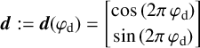 $$ \begin{align*} \boldsymbol{d} := \boldsymbol{d}(\varphi_{\mathrm{d}}) = \left[ \begin{array}{@{}c@{}} \cos{(2 \pi\, \varphi_{\mathrm{d}})} \\[0.5mm] \sin{(2 \pi\, \varphi_{\mathrm{d}})} \end{array} \right] \end{align*} $$
for any direction angle $\varphi _{\mathrm {d}} \in [0, 1)$
. (Here and throughout, we consider Euclidean distance.) The definition of
$\varphi _{\mathrm {d}} \in [0, 1)$
. (Here and throughout, we consider Euclidean distance.) The definition of $\mathcal {P}_A$
can then be extended to the domain
$\mathcal {P}_A$
can then be extended to the domain
 $$ \begin{align*} \mathcal{P}_A: [0,1) \times [0, 1) \to [0,1); \quad (\vartheta_\mathrm{o} , \varphi_\mathrm{d}) \mapsto \vartheta_\mathrm{n}, \end{align*} $$
where the image $\vartheta _{\mathrm {n}}$
is given by the phase of the isochron that contains the point
$\vartheta _{\mathrm {n}}$
is given by the phase of the isochron that contains the point $\gamma (\vartheta _{\mathrm {o}}) + A \, \boldsymbol {d}(\varphi _{\mathrm {d}})$
, resulting from a reset at the point
$\gamma (\vartheta _{\mathrm {o}}) + A \, \boldsymbol {d}(\varphi _{\mathrm {d}})$
, resulting from a reset at the point $\gamma (\vartheta _{\mathrm {o}}) \in \Gamma $
.
$\gamma (\vartheta _{\mathrm {o}}) \in \Gamma $
.
For $\varphi _{\mathrm {d}} = 0$
, the unit vector
$\varphi _{\mathrm {d}} = 0$
, the unit vector $\boldsymbol {d}(\varphi _{\mathrm {d}})$
is exclusively in the direction of positive x only, which is the case we considered in Section 3. The entire transition scenario of the PTC from
$\boldsymbol {d}(\varphi _{\mathrm {d}})$
is exclusively in the direction of positive x only, which is the case we considered in Section 3. The entire transition scenario of the PTC from $1\! : \!1$
to
$1\! : \!1$
to $1\! : \!0$
torus knot we presented is generated solely by the fact that the perturbation set of the periodic orbit moves through the phaseless point
$1\! : \!0$
torus knot we presented is generated solely by the fact that the perturbation set of the periodic orbit moves through the phaseless point $\boldsymbol {x}^*$
as the perturbation amplitude is increased through the critical amplitude
$\boldsymbol {x}^*$
as the perturbation amplitude is increased through the critical amplitude $A_c$
. For
$A_c$
. For $\varphi _{\mathrm {d}} = 0$
, this happens at
$\varphi _{\mathrm {d}} = 0$
, this happens at $A = A_c \approx 0.4041$
and at the unique point
$A = A_c \approx 0.4041$
and at the unique point $\gamma (\vartheta _{\mathrm {o}}) \in \Gamma $
of phase
$\gamma (\vartheta _{\mathrm {o}}) \in \Gamma $
of phase $\vartheta _{\mathrm {o}} \approx 0.3484$
. However, since
$\vartheta _{\mathrm {o}} \approx 0.3484$
. However, since $\Gamma $
surrounds
$\Gamma $
surrounds $\boldsymbol {x}^*$
, this will also happen for an increasing perturbation amplitude in any direction, albeit for a different value of the critical amplitude
$\boldsymbol {x}^*$
, this will also happen for an increasing perturbation amplitude in any direction, albeit for a different value of the critical amplitude $A_c$
and at a different phase
$A_c$
and at a different phase $\vartheta _{\mathrm {o}}$
.
$\vartheta _{\mathrm {o}}$
.
Figure 6 illustrates how the critical perturbation amplitude $A_c$
depends on the perturbation direction
$A_c$
depends on the perturbation direction $\boldsymbol {d}(\varphi _{\mathrm {d}})$
, with
$\boldsymbol {d}(\varphi _{\mathrm {d}})$
, with $\varphi _{\mathrm {d}} \in [0, 1)$
, and the phase
$\varphi _{\mathrm {d}} \in [0, 1)$
, and the phase $\vartheta _{\mathrm {o}} \in [0, 1)$
at which the reset is applied. Panel (a) shows
$\vartheta _{\mathrm {o}} \in [0, 1)$
at which the reset is applied. Panel (a) shows $\Gamma $
together with 50 isochrons evenly distributed in phase. We labelled four points on
$\Gamma $
together with 50 isochrons evenly distributed in phase. We labelled four points on $\Gamma $
, which are local extrema of the pointwise distance between
$\Gamma $
, which are local extrema of the pointwise distance between $\Gamma $
and
$\Gamma $
and $\boldsymbol {x}^*$
. Observe that for any
$\boldsymbol {x}^*$
. Observe that for any $\vartheta _{\mathrm {o}} \in [0, 1)$
, the point
$\vartheta _{\mathrm {o}} \in [0, 1)$
, the point $\gamma (\vartheta _{\mathrm {o}}) \in \Gamma $
is shifted exactly to
$\gamma (\vartheta _{\mathrm {o}}) \in \Gamma $
is shifted exactly to $\boldsymbol {x}^*$
by the vector
$\boldsymbol {x}^*$
by the vector $\boldsymbol {x}^* - \gamma (\vartheta _{\mathrm {o}})$
; in other words,
$\boldsymbol {x}^* - \gamma (\vartheta _{\mathrm {o}})$
; in other words, $\gamma (\vartheta _{\mathrm {o}})$
resets to
$\gamma (\vartheta _{\mathrm {o}})$
resets to $\boldsymbol {x}^*$
for the perturbation with amplitude
$\boldsymbol {x}^*$
for the perturbation with amplitude $A_c = ||\boldsymbol {x}^* - \gamma (\vartheta _{\mathrm {o}})||$
in the unique direction
$A_c = ||\boldsymbol {x}^* - \gamma (\vartheta _{\mathrm {o}})||$
in the unique direction $\boldsymbol {d} = (\boldsymbol {x}^* - \gamma (\vartheta _{\mathrm {o}})) / ||\boldsymbol {x}^* - \gamma (\vartheta _{\mathrm {o}})||$
. In particular, the critical perturbation amplitude
$\boldsymbol {d} = (\boldsymbol {x}^* - \gamma (\vartheta _{\mathrm {o}})) / ||\boldsymbol {x}^* - \gamma (\vartheta _{\mathrm {o}})||$
. In particular, the critical perturbation amplitude $A_c$
achieves a local maximum or minimum when viewed as a function of
$A_c$
achieves a local maximum or minimum when viewed as a function of $\vartheta _{\mathrm {o}}$
or, alternatively, as a function of the angle
$\vartheta _{\mathrm {o}}$
or, alternatively, as a function of the angle $\varphi _{\mathrm {d}}$
of
$\varphi _{\mathrm {d}}$
of $\boldsymbol {d}$
as defined above. These two graphs are also shown in Figure 6:
$\boldsymbol {d}$
as defined above. These two graphs are also shown in Figure 6: $A_c$
as a function of
$A_c$
as a function of $\vartheta _{\mathrm {o}} \in [0, 1)$
in panel (b) and
$\vartheta _{\mathrm {o}} \in [0, 1)$
in panel (b) and $A_c$
as a function of
$A_c$
as a function of $\varphi _{\mathrm {d}} \in [0, 1)$
in panel (c). The extrema of each graph have the same
$\varphi _{\mathrm {d}} \in [0, 1)$
in panel (c). The extrema of each graph have the same $A_c$
-values and we first discuss how they divide the
$A_c$
-values and we first discuss how they divide the $A_c$
-axis into five different ranges. Section 4.1 then presents and discusses the corresponding five phase-resetting surfaces, which are shown in Figures 7–11.
$A_c$
-axis into five different ranges. Section 4.1 then presents and discusses the corresponding five phase-resetting surfaces, which are shown in Figures 7–11.
Determining the critical perturbation amplitude $A_c$
. Panel (a) shows
$A_c$
. Panel (a) shows $\Gamma $
(black curve) with 50 isochrons evenly distributed in phase and the points labelled
$\Gamma $
(black curve) with 50 isochrons evenly distributed in phase and the points labelled $f_1$
,
$f_1$
, $f^*_1$
(blue) and
$f^*_1$
(blue) and $f_2$
,
$f_2$
, $f^*_2$
(red) marked on
$f^*_2$
(red) marked on $\Gamma $
that lie respectively at (locally) minimal and maximal distances from the source
$\Gamma $
that lie respectively at (locally) minimal and maximal distances from the source $\boldsymbol {x}^*$
. Panels (b) and (c) show the graphs of
$\boldsymbol {x}^*$
. Panels (b) and (c) show the graphs of $A_c$
as a function of
$A_c$
as a function of $\vartheta _{\mathrm {o}}$
and
$\vartheta _{\mathrm {o}}$
and $\varphi _{\mathrm {d}}$
, respectively, with the branches labelled
$\varphi _{\mathrm {d}}$
, respectively, with the branches labelled $s_1$
,
$s_1$
, $s_1^*$
,
$s_1^*$
, $s_2$
and
$s_2$
and $s_2^*$
giving the values of
$s_2^*$
giving the values of $\vartheta _{\mathrm {o}}$
and
$\vartheta _{\mathrm {o}}$
and $\varphi _{\mathrm {d}}$
that achieve singular phase resets for a chosen
$\varphi _{\mathrm {d}}$
that achieve singular phase resets for a chosen $A_c$
; the three horizontal lines at
$A_c$
; the three horizontal lines at $A = 0.35$
,
$A = 0.35$
, $A = 0.6$
and
$A = 0.6$
and $A = 0.95$
thus identify the singular points shown in Figures 8, 9 and 10, respectively.
$A = 0.95$
thus identify the singular points shown in Figures 8, 9 and 10, respectively.
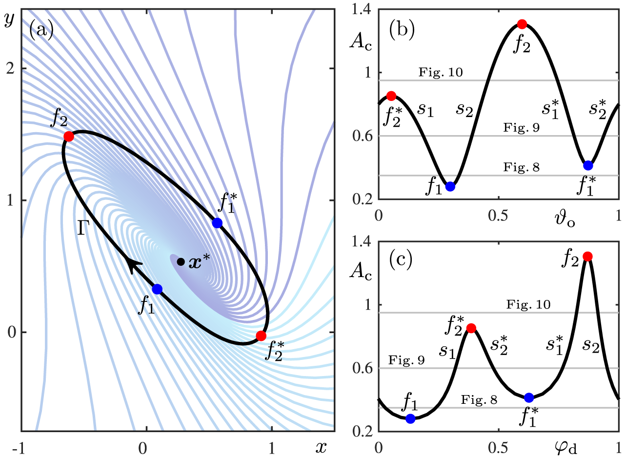
The critical perturbation amplitude has a global minimum of $A_c \approx 0.2805$
, at
$A_c \approx 0.2805$
, at $\vartheta _{\mathrm {o}} \approx 0.2981$
and at
$\vartheta _{\mathrm {o}} \approx 0.2981$
and at $\varphi _{\mathrm {d}} \approx 0.1324$
, given by the points labelled
$\varphi _{\mathrm {d}} \approx 0.1324$
, given by the points labelled $f_1$
in panels (a), (b) and (c) of Figure 6. Hence, any phase reset, in any direction, with perturbation amplitude
$f_1$
in panels (a), (b) and (c) of Figure 6. Hence, any phase reset, in any direction, with perturbation amplitude $0 \leq A < 0.2805$
, leads to a PTC that is a
$0 \leq A < 0.2805$
, leads to a PTC that is a $1\! : \!1$
torus knot, because the effect is a small shift of
$1\! : \!1$
torus knot, because the effect is a small shift of $\Gamma $
that involves no interaction with
$\Gamma $
that involves no interaction with $\boldsymbol {x}^*$
. Similarly,
$\boldsymbol {x}^*$
. Similarly, $A_c$
has a global maximum of
$A_c$
has a global maximum of $A_c \approx 1.3051$
, labelled
$A_c \approx 1.3051$
, labelled $f_2$
in Figure 6, at
$f_2$
in Figure 6, at $\vartheta _{\mathrm {o}} \approx 0.5971$
and at
$\vartheta _{\mathrm {o}} \approx 0.5971$
and at $\varphi _{\mathrm {d}} \approx 0.8702$
. Any phase reset, in any direction, with perturbation amplitude
$\varphi _{\mathrm {d}} \approx 0.8702$
. Any phase reset, in any direction, with perturbation amplitude $A> 1.3051$
leads to a PTC that is a
$A> 1.3051$
leads to a PTC that is a $1\! : \!0$
torus knot, because the perturbed orbit no longer encloses
$1\! : \!0$
torus knot, because the perturbed orbit no longer encloses $\boldsymbol {x}^*$
. However, for any perturbation amplitude A in the range
$\boldsymbol {x}^*$
. However, for any perturbation amplitude A in the range $[0.2805, 1.3051]$
, there exists a direction angle
$[0.2805, 1.3051]$
, there exists a direction angle $\varphi _{\mathrm {d}} \in [0, 1)$
such that PTC has a discontinuity; this direction angle is generically not unique.
$\varphi _{\mathrm {d}} \in [0, 1)$
such that PTC has a discontinuity; this direction angle is generically not unique.
Three copies of the phase-resetting surface $\mathrm {graph}(\mathcal {P}_A)$
of system (2.1) shown in
$\mathrm {graph}(\mathcal {P}_A)$
of system (2.1) shown in $(\vartheta _{\mathrm {o}}, \varphi _{\mathrm {d}}, \vartheta _{\mathrm {n}})$
-space for
$(\vartheta _{\mathrm {o}}, \varphi _{\mathrm {d}}, \vartheta _{\mathrm {n}})$
-space for $\vartheta _{\mathrm {n}} \in [-0.5, 2.5]$
with
$\vartheta _{\mathrm {n}} \in [-0.5, 2.5]$
with $A = 0.2$
.
$A = 0.2$
.
Panel (a) shows three copies of the phase-resetting surface $\mathrm {graph}(\mathcal {P}_A)$
of system (2.1) in
$\mathrm {graph}(\mathcal {P}_A)$
of system (2.1) in $(\vartheta _{\mathrm {o}}, \varphi _{\mathrm {d}}, \vartheta _{\mathrm {n}})$
-space for
$(\vartheta _{\mathrm {o}}, \varphi _{\mathrm {d}}, \vartheta _{\mathrm {n}})$
-space for $\vartheta _{\mathrm {n}} \in [-0.5, 2.5]$
with
$\vartheta _{\mathrm {n}} \in [-0.5, 2.5]$
with $A = 0.35$
, featuring two singularities
$A = 0.35$
, featuring two singularities $s_1$
and
$s_1$
and $s_2$
(grey vertical lines); also shown are the two PTCs for
$s_2$
(grey vertical lines); also shown are the two PTCs for $\varphi _{\mathrm {d}} = 0.2$
(purple) and
$\varphi _{\mathrm {d}} = 0.2$
(purple) and $\varphi _{\mathrm {d}} = 0.5$
(orange). Panel (b) is a projection of panel (a) onto the
$\varphi _{\mathrm {d}} = 0.5$
(orange). Panel (b) is a projection of panel (a) onto the $(\vartheta _{\mathrm {o}}, {\varphi _{\mathrm {d}}})$
-plane and panel (c) shows the two PTCs on the fundamental square (green shading) of the
$(\vartheta _{\mathrm {o}}, {\varphi _{\mathrm {d}}})$
-plane and panel (c) shows the two PTCs on the fundamental square (green shading) of the $(\vartheta _{\mathrm {o}}, \vartheta _{\mathrm {n}})$
-plane.
$(\vartheta _{\mathrm {o}}, \vartheta _{\mathrm {n}})$
-plane.
Panel (a) shows three copies of the phase-resetting surface $\mathrm {graph}(\mathcal {P}_A)$
of system (2.1) in
$\mathrm {graph}(\mathcal {P}_A)$
of system (2.1) in $(\vartheta _{\mathrm {o}}, \varphi _{\mathrm {d}}, \vartheta _{\mathrm {n}})$
-space for
$(\vartheta _{\mathrm {o}}, \varphi _{\mathrm {d}}, \vartheta _{\mathrm {n}})$
-space for $\vartheta _{\mathrm {n}} \in [-0.5, 2.5]$
with
$\vartheta _{\mathrm {n}} \in [-0.5, 2.5]$
with $A = 0.6$
, featuring four singularities
$A = 0.6$
, featuring four singularities $s_1$
,
$s_1$
, $s_2$
,
$s_2$
, $s_1^*$
and
$s_1^*$
and $s_2^*$
(grey vertical lines); also shown are the four PTCs for
$s_2^*$
(grey vertical lines); also shown are the four PTCs for $\varphi _{\mathrm {d}} = 0.2$
(orange),
$\varphi _{\mathrm {d}} = 0.2$
(orange), $\varphi _{\mathrm {d}} = 0.4$
(purple),
$\varphi _{\mathrm {d}} = 0.4$
(purple), $\varphi _{\mathrm {d}} = 0.55$
(red) and
$\varphi _{\mathrm {d}} = 0.55$
(red) and $\varphi _{\mathrm {d}} = 0.8$
(blue). Panel (b) is a projection of panel (a) onto the
$\varphi _{\mathrm {d}} = 0.8$
(blue). Panel (b) is a projection of panel (a) onto the $(\vartheta _{\mathrm {o}}, \varphi _{\mathrm {d}})$
-plane and panel (c) shows the four PTCs on the fundamental square (green shading) of the
$(\vartheta _{\mathrm {o}}, \varphi _{\mathrm {d}})$
-plane and panel (c) shows the four PTCs on the fundamental square (green shading) of the $(\vartheta _{\mathrm {o}}, \vartheta _{\mathrm {n}})$
-plane.
$(\vartheta _{\mathrm {o}}, \vartheta _{\mathrm {n}})$
-plane.
Panel (a) shows three copies of the phase-resetting surface $\mathrm {graph}(\mathcal {P}_A)$
of system (2.1) in
$\mathrm {graph}(\mathcal {P}_A)$
of system (2.1) in $(\vartheta _{\mathrm {o}}, \varphi _{\mathrm {d}}, \vartheta _{\mathrm {n}})$
-space for
$(\vartheta _{\mathrm {o}}, \varphi _{\mathrm {d}}, \vartheta _{\mathrm {n}})$
-space for $\vartheta _{\mathrm {n}} \in [-0.5, 2.5]$
with
$\vartheta _{\mathrm {n}} \in [-0.5, 2.5]$
with $A = 0.95$
, featuring two singularities
$A = 0.95$
, featuring two singularities $s_1^*$
and
$s_1^*$
and $s_2$
(grey vertical lines); also shown are the two PTCs for
$s_2$
(grey vertical lines); also shown are the two PTCs for $\varphi _{\mathrm {d}} = 0.5$
(red) and
$\varphi _{\mathrm {d}} = 0.5$
(red) and $\varphi _{\mathrm {d}} = 0.85$
(blue). Panel (b) is a projection of panel (a) onto the
$\varphi _{\mathrm {d}} = 0.85$
(blue). Panel (b) is a projection of panel (a) onto the $(\vartheta _{\mathrm {o}}, {\varphi _{\mathrm {d}}})$
-plane and panel (c) shows the two PTCs on the fundamental square (green shading) of the
$(\vartheta _{\mathrm {o}}, {\varphi _{\mathrm {d}}})$
-plane and panel (c) shows the two PTCs on the fundamental square (green shading) of the $(\vartheta _{\mathrm {o}}, \vartheta _{\mathrm {n}})$
-plane.
$(\vartheta _{\mathrm {o}}, \vartheta _{\mathrm {n}})$
-plane.
Three copies of the phase-resetting surface $\mathrm {graph}(\mathcal {P}_A)$
of system (2.1) shown in
$\mathrm {graph}(\mathcal {P}_A)$
of system (2.1) shown in $(\vartheta _{\mathrm {o}}, \varphi _{\mathrm {d}}, \vartheta _{\mathrm {n}})$
-space for
$(\vartheta _{\mathrm {o}}, \varphi _{\mathrm {d}}, \vartheta _{\mathrm {n}})$
-space for $\vartheta _{\mathrm {n}} \in [-0.5, 2.5]$
with
$\vartheta _{\mathrm {n}} \in [-0.5, 2.5]$
with $A = 0.95$
.
$A = 0.95$
.
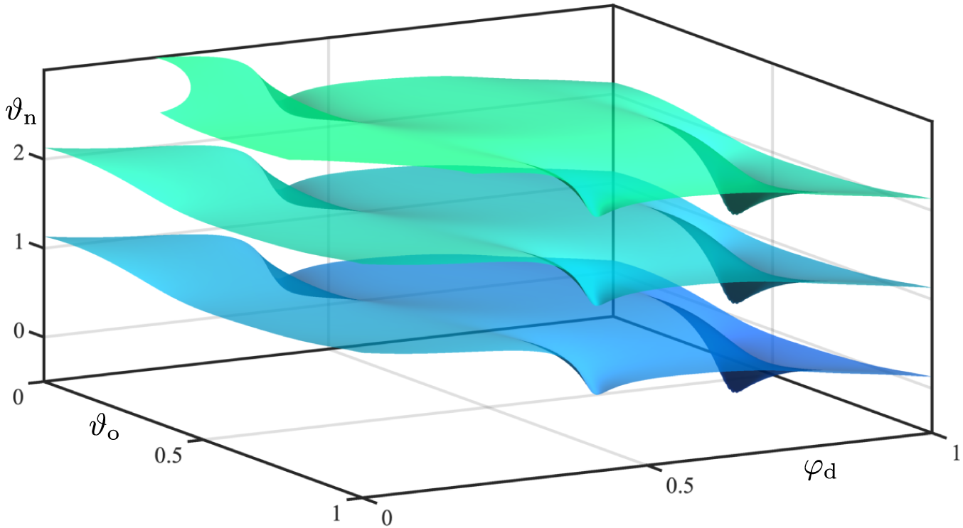
The existing pairs $(\vartheta _{\mathrm {o}}, \varphi _{\mathrm {d}})$
that lead to a singular phase reset are given by the intersection points of the graphs in Figures 6(b) and 6(c) with a horizontal line at the selected value of
$(\vartheta _{\mathrm {o}}, \varphi _{\mathrm {d}})$
that lead to a singular phase reset are given by the intersection points of the graphs in Figures 6(b) and 6(c) with a horizontal line at the selected value of $A_c$
; each such intersection point lies on one of four branches labelled
$A_c$
; each such intersection point lies on one of four branches labelled $s_1$
,
$s_1$
, $s_2$
,
$s_2$
, $s_1^*$
and
$s_1^*$
and $s_2^*$
. How many there are depends on the level of
$s_2^*$
. How many there are depends on the level of $A_c$
relative to the two other extremal points
$A_c$
relative to the two other extremal points $f^*_1$
and
$f^*_1$
and $f^*_2$
: a local minimum and a local maximum of the distance from
$f^*_2$
: a local minimum and a local maximum of the distance from $\boldsymbol {x}^*$
of
$\boldsymbol {x}^*$
of $A_c \approx 0.4134$
and
$A_c \approx 0.4134$
and $A_c \approx 0.8519$
, respectively. For any phase reset with perturbation amplitude A in the range
$A_c \approx 0.8519$
, respectively. For any phase reset with perturbation amplitude A in the range $(0.2805, 0.4134)$
, the horizontal line with
$(0.2805, 0.4134)$
, the horizontal line with $A_c = A$
intersects only the branches
$A_c = A$
intersects only the branches $s_1$
and
$s_1$
and $s_2$
; for
$s_2$
; for $A \in (0.4134, 0.8519)$
, it intersects all four branches; and for
$A \in (0.4134, 0.8519)$
, it intersects all four branches; and for $A \in (0.8519, 1.3051)$
, it intersects only the branches
$A \in (0.8519, 1.3051)$
, it intersects only the branches $s_2$
and
$s_2$
and $s_1^*$
. Hence, in these ranges, there are two, four and again two particular phases along
$s_1^*$
. Hence, in these ranges, there are two, four and again two particular phases along $\Gamma $
that reset to
$\Gamma $
that reset to $\boldsymbol {x}^*$
, provided the associated specific direction angle
$\boldsymbol {x}^*$
, provided the associated specific direction angle $\varphi _{\mathrm {d}} \in [0, 1)$
is selected. Each such reset to
$\varphi _{\mathrm {d}} \in [0, 1)$
is selected. Each such reset to $\boldsymbol {x}^*$
corresponds to a singularity where the phase reset is not defined; the three horizontal lines indicate the representative values of A we chose in Figures 8–10 to present the corresponding phase-resetting surfaces with singularities.
$\boldsymbol {x}^*$
corresponds to a singularity where the phase reset is not defined; the three horizontal lines indicate the representative values of A we chose in Figures 8–10 to present the corresponding phase-resetting surfaces with singularities.
4.1 Phase-resetting surface for fixed A
To illustrate the influence of the direction $\boldsymbol {d}$
of the perturbation, we now consider
$\boldsymbol {d}$
of the perturbation, we now consider $\mathrm {graph}(\mathcal {P}_A)$
in
$\mathrm {graph}(\mathcal {P}_A)$
in $(\vartheta _{\mathrm {o}}, \varphi _{\mathrm {d}}, \vartheta _{\mathrm {n}})$
-space for different values of the perturbation amplitude A. As we discussed above, there are five different generic cases, corresponding to the five A-ranges generated by the values of
$(\vartheta _{\mathrm {o}}, \varphi _{\mathrm {d}}, \vartheta _{\mathrm {n}})$
-space for different values of the perturbation amplitude A. As we discussed above, there are five different generic cases, corresponding to the five A-ranges generated by the values of $A_c$
at the four extrema
$A_c$
at the four extrema $f_1$
,
$f_1$
, $f^*_1$
,
$f^*_1$
, $f_2$
and
$f_2$
and $f^*_2$
. They are presented in Figures 7–11, where we show three copies or sheets of
$f^*_2$
. They are presented in Figures 7–11, where we show three copies or sheets of $\mathrm {graph}(\mathcal {P}_A)$
over the extended
$\mathrm {graph}(\mathcal {P}_A)$
over the extended $\vartheta _{\mathrm {n}}$
-range
$\vartheta _{\mathrm {n}}$
-range $[-0.5, 2.5]$
.
$[-0.5, 2.5]$
.
Figure 7 shows the phase-resetting surface $\mathrm {graph}(\mathcal {P}_A)$
for
$\mathrm {graph}(\mathcal {P}_A)$
for $A = 0.2$
, representing the A-interval
$A = 0.2$
, representing the A-interval $[0, 0.2805)$
. Here, the PTC for any
$[0, 0.2805)$
. Here, the PTC for any $\varphi _{\mathrm {d}}$
is a
$\varphi _{\mathrm {d}}$
is a $1\! : \!1$
torus knot, which means that the three sheets of
$1\! : \!1$
torus knot, which means that the three sheets of $\mathrm {graph}(\mathcal {P}_A)$
are tilted so that the value of
$\mathrm {graph}(\mathcal {P}_A)$
are tilted so that the value of $\vartheta _{\mathrm {n}}$
increases by
$\vartheta _{\mathrm {n}}$
increases by $1$
as
$1$
as $\vartheta _{\mathrm {o}}$
varies from
$\vartheta _{\mathrm {o}}$
varies from $0$
to
$0$
to $1$
.
$1$
.
Figure 8 shows the situation for $A = 0.35$
, representing
$A = 0.35$
, representing $A \in (0.2805, 0.4134)$
. Panel (a) shows three sheets of
$A \in (0.2805, 0.4134)$
. Panel (a) shows three sheets of $\mathrm {graph}(\mathcal {P}_A)$
in
$\mathrm {graph}(\mathcal {P}_A)$
in $(\vartheta _{\mathrm {o}}, \varphi _{\mathrm {d}}, \vartheta _{\mathrm {n}})$
-space with the PTCs for the
$(\vartheta _{\mathrm {o}}, \varphi _{\mathrm {d}}, \vartheta _{\mathrm {n}})$
-space with the PTCs for the $\varphi _{\mathrm {d}}$
-values
$\varphi _{\mathrm {d}}$
-values $0.2$
and
$0.2$
and $0.5$
, panel (b) provides a “top-down” view in projection onto the
$0.5$
, panel (b) provides a “top-down” view in projection onto the $(\vartheta _{\mathrm {o}}, \varphi _{\mathrm {d}})$
-plane, and the two PTCs are shown in panel (c) on the fundamental square. As Figure 8(a) shows, the three sheets of
$(\vartheta _{\mathrm {o}}, \varphi _{\mathrm {d}})$
-plane, and the two PTCs are shown in panel (c) on the fundamental square. As Figure 8(a) shows, the three sheets of $\mathrm {graph}(\mathcal {P}_A)$
now all wrap around two singular vertical lines labelled
$\mathrm {graph}(\mathcal {P}_A)$
now all wrap around two singular vertical lines labelled $s_1$
and
$s_1$
and $s_2$
; these singularities are at
$s_2$
; these singularities are at $(\vartheta _{\mathrm {o}},\varphi _{\mathrm {d}}) \approx (0.2585, 0.2372)$
and
$(\vartheta _{\mathrm {o}},\varphi _{\mathrm {d}}) \approx (0.2585, 0.2372)$
and $(\vartheta _{\mathrm {o}},\varphi _{\mathrm {d}}) \approx (0.3346, 0.0258)$
, and they are created, for increasing A, when the global minimum
$(\vartheta _{\mathrm {o}},\varphi _{\mathrm {d}}) \approx (0.3346, 0.0258)$
, and they are created, for increasing A, when the global minimum $f_1$
at
$f_1$
at $A_c \approx 0.2805$
is passed in Figures 6(b) and 6(c), so that the branches
$A_c \approx 0.2805$
is passed in Figures 6(b) and 6(c), so that the branches $s_1$
and
$s_1$
and $s_2$
are intersected. As Figure 8(b) illustrates with a top view, there is now the “window”
$s_2$
are intersected. As Figure 8(b) illustrates with a top view, there is now the “window” $(0.0258,0.2372)$
of
$(0.0258,0.2372)$
of $\varphi _{\mathrm {d}}$
-values in between their “singular” values corresponding to
$\varphi _{\mathrm {d}}$
-values in between their “singular” values corresponding to $s_1$
and
$s_1$
and $s_2$
, for which the PTC is already a
$s_2$
, for which the PTC is already a $1\! : \!0$
torus knot; for the complement
$1\! : \!0$
torus knot; for the complement $\varphi _{\mathrm {d}} \in [0,1) \setminus [0.0258,0.2372]$
, the PTC is still a
$\varphi _{\mathrm {d}} \in [0,1) \setminus [0.0258,0.2372]$
, the PTC is still a $1\! : \!1$
torus knot. The PTCs for
$1\! : \!1$
torus knot. The PTCs for $\varphi _{\mathrm {d}} = 0.2$
and
$\varphi _{\mathrm {d}} = 0.2$
and $\varphi _{\mathrm {d}} = 0.5$
in panel (c) are representative examples of these two cases. Exactly for the
$\varphi _{\mathrm {d}} = 0.5$
in panel (c) are representative examples of these two cases. Exactly for the $\varphi _{\mathrm {d}}$
-values of the singularities
$\varphi _{\mathrm {d}}$
-values of the singularities $s_1$
and
$s_1$
and $s_2$
, the PTC has a discontinuity as the one for
$s_2$
, the PTC has a discontinuity as the one for $A = A_c$
shown in Figure 1(b).
$A = A_c$
shown in Figure 1(b).
Figure 9 shows the phase-resetting surface $\mathrm {graph}(\mathcal {P}_A)$
for
$\mathrm {graph}(\mathcal {P}_A)$
for $A = 0.6$
, which is representative for the A-interval
$A = 0.6$
, which is representative for the A-interval $(0.4134, 0.8519)$
, where one finds the four singularities
$(0.4134, 0.8519)$
, where one finds the four singularities $s_1$
,
$s_1$
, $s_2$
,
$s_2$
, $s_1^*$
and
$s_1^*$
and $s_2^*$
. Consequently, PTCs without discontinuities for this A-range are found in four
$s_2^*$
. Consequently, PTCs without discontinuities for this A-range are found in four $\varphi _{\mathrm {d}}$
-ranges. The singularities
$\varphi _{\mathrm {d}}$
-ranges. The singularities $s_1$
and
$s_1$
and $s_2$
are now at
$s_2$
are now at $(\vartheta _{\mathrm {o}},\varphi _{\mathrm { d}}) \approx (0.1857, 0.3188)$
and
$(\vartheta _{\mathrm {o}},\varphi _{\mathrm { d}}) \approx (0.1857, 0.3188)$
and $(\vartheta _{\mathrm {o}},\varphi _{\mathrm {d}}) \approx (0.3883, 0.9508)$
, respectively. Moreover, there are two additional singularities
$(\vartheta _{\mathrm {o}},\varphi _{\mathrm {d}}) \approx (0.3883, 0.9508)$
, respectively. Moreover, there are two additional singularities $s_1^*$
and
$s_1^*$
and $s_2^*$
at
$s_2^*$
at $(\vartheta _{\mathrm {o}},\varphi _{\mathrm {d}}) \approx (0.7651, 0.8135)$
and
$(\vartheta _{\mathrm {o}},\varphi _{\mathrm {d}}) \approx (0.7651, 0.8135)$
and $(\vartheta _{\mathrm {o}},\varphi _{\mathrm {d}}) \approx (0.9368, 0.4768)$
, respectively. The phase-resetting surface
$(\vartheta _{\mathrm {o}},\varphi _{\mathrm {d}}) \approx (0.9368, 0.4768)$
, respectively. The phase-resetting surface $\mathrm {graph}(\mathcal {P}_A)$
in Figure 9(a) now wraps around all four singular vertical lines
$\mathrm {graph}(\mathcal {P}_A)$
in Figure 9(a) now wraps around all four singular vertical lines $s_1$
,
$s_1$
, $s_2$
,
$s_2$
, $s_1^*$
and
$s_1^*$
and $s_2^*$
. Resets in directions corresponding to the associated singular
$s_2^*$
. Resets in directions corresponding to the associated singular $\varphi _{\mathrm {d}}$
-values lead to discontinuous PTCs. As the top view in panel (b) shows, there are now two “windows” of
$\varphi _{\mathrm {d}}$
-values lead to discontinuous PTCs. As the top view in panel (b) shows, there are now two “windows” of $\varphi _{\mathrm {d}}$
-values for which the PTC is already a
$\varphi _{\mathrm {d}}$
-values for which the PTC is already a $1\! : \!0$
torus knot: the one between
$1\! : \!0$
torus knot: the one between $s_1$
and
$s_1$
and $s_2$
for
$s_2$
for $\varphi _{\mathrm {d}} \in (0.9508 - 1,0.3188)$
, which is wider than in Figure 7, and there is also a second window between
$\varphi _{\mathrm {d}} \in (0.9508 - 1,0.3188)$
, which is wider than in Figure 7, and there is also a second window between $s_1^*$
and
$s_1^*$
and $s_2^*$
for
$s_2^*$
for $\varphi _{\mathrm {d}} \in (0.4768, 0.8135)$
. The PTCs for
$\varphi _{\mathrm {d}} \in (0.4768, 0.8135)$
. The PTCs for $\varphi _{\mathrm {d}} = 0.2$
and
$\varphi _{\mathrm {d}} = 0.2$
and $\varphi _{\mathrm {d}} = 0.55$
in Figure 9(c) are representative examples for these two
$\varphi _{\mathrm {d}} = 0.55$
in Figure 9(c) are representative examples for these two $\varphi _{\mathrm {d}}$
-ranges of
$\varphi _{\mathrm {d}}$
-ranges of $1\! : \!0$
torus knots. In the two complementary
$1\! : \!0$
torus knots. In the two complementary $\varphi _{\mathrm {d}}$
-ranges, however, the PTC is still a
$\varphi _{\mathrm {d}}$
-ranges, however, the PTC is still a $1\! : \!1$
torus knot, such as the PTCs for
$1\! : \!1$
torus knot, such as the PTCs for $\varphi _{\mathrm {d}} = 0.4$
and
$\varphi _{\mathrm {d}} = 0.4$
and $\varphi _{\mathrm {d}} = 0.8$
in panel (c).
$\varphi _{\mathrm {d}} = 0.8$
in panel (c).
As A is increased, the singular points $s_1$
and
$s_1$
and $s^*_2$
move closer together, and they merge and disappear at the local maximum
$s^*_2$
move closer together, and they merge and disappear at the local maximum $f^*_2$
at
$f^*_2$
at $A_c \approx 0.8519$
. Figure 10(a) shows the phase-resetting surface
$A_c \approx 0.8519$
. Figure 10(a) shows the phase-resetting surface $\mathrm {graph}(\mathcal {P}_A)$
for
$\mathrm {graph}(\mathcal {P}_A)$
for $A = 0.95$
, which is representative for the A-interval
$A = 0.95$
, which is representative for the A-interval $(0.8519, 1.3051)$
. Again, only two singularities remain, namely,
$(0.8519, 1.3051)$
. Again, only two singularities remain, namely, $s_1^*$
and
$s_1^*$
and $s_2$
at
$s_2$
at $(0.7445, 0.8236)$
and
$(0.7445, 0.8236)$
and $(0.4559, 0.9126)$
, respectively. The geometry of the phase-resetting surface
$(0.4559, 0.9126)$
, respectively. The geometry of the phase-resetting surface $\mathrm {graph}(\mathcal {P}_A)$
in panel (a) looks again like that in Figure 8(a), but the difference is that the PTC is now a
$\mathrm {graph}(\mathcal {P}_A)$
in panel (a) looks again like that in Figure 8(a), but the difference is that the PTC is now a $1\! : \!0$
torus knot for almost all values of
$1\! : \!0$
torus knot for almost all values of $\varphi _{\mathrm {d}}$
, except for the
$\varphi _{\mathrm {d}}$
, except for the $\varphi _{\mathrm {d}}$
-range
$\varphi _{\mathrm {d}}$
-range $(0.8236, 0.9126)$
in between
$(0.8236, 0.9126)$
in between $s_1^*$
and
$s_1^*$
and $s_2$
; see Figures 10(b) and 10(c) for the two PTCs for the
$s_2$
; see Figures 10(b) and 10(c) for the two PTCs for the $\varphi _{\mathrm {d}}$
-values
$\varphi _{\mathrm {d}}$
-values $0.5$
and
$0.5$
and $0.85$
that are representatives of these two cases.
$0.85$
that are representatives of these two cases.
As A is increased further through the global maximum $f_2$
at
$f_2$
at $A_c \approx 1.3051$
, also
$A_c \approx 1.3051$
, also $s_1^*$
and
$s_1^*$
and $s_2$
disappear and
$s_2$
disappear and $\mathrm {graph}(\mathcal {P}_A)$
is as shown in Figure 11 for the representative value
$\mathrm {graph}(\mathcal {P}_A)$
is as shown in Figure 11 for the representative value $A = 1.4$
. Here, the three sheets shown are such that there is no increase of
$A = 1.4$
. Here, the three sheets shown are such that there is no increase of $\vartheta _{\mathrm {n}}$
when
$\vartheta _{\mathrm {n}}$
when $\vartheta _{\mathrm {o}}$
varies from
$\vartheta _{\mathrm {o}}$
varies from $0$
to
$0$
to $1$
and, hence, all PTCs are
$1$
and, hence, all PTCs are $1\! : \!0$
torus knots. Notice, however, that the three sheets are just tilted differently compared with the three sheets in Figure 7, for which all PTCs are
$1\! : \!0$
torus knots. Notice, however, that the three sheets are just tilted differently compared with the three sheets in Figure 7, for which all PTCs are $1\! : \!1$
torus knots. In Figure 11, the value of
$1\! : \!1$
torus knots. In Figure 11, the value of $\vartheta _{\mathrm {n}}$
increases by one as the direction angle
$\vartheta _{\mathrm {n}}$
increases by one as the direction angle $\varphi _{\mathrm {d}}$
, rather than the old phase
$\varphi _{\mathrm {d}}$
, rather than the old phase $\vartheta _{\mathrm {o}}$
, varies from
$\vartheta _{\mathrm {o}}$
, varies from $0$
to
$0$
to $1$
.
$1$
.
5 Conclusion and outlook
We studied phase resetting in the FitzHugh–Nagumo system (2.1), with a stable periodic orbit $\Gamma $
surrounding a repelling focus
$\Gamma $
surrounding a repelling focus $\boldsymbol {x}^*$
, which is the only point not in the basin of attraction. Perturbations at phase
$\boldsymbol {x}^*$
, which is the only point not in the basin of attraction. Perturbations at phase $\vartheta _{\mathrm {o}}$
, with amplitude A and in the direction
$\vartheta _{\mathrm {o}}$
, with amplitude A and in the direction $\boldsymbol {d}({\varphi }_d)$
, result in a new phase
$\boldsymbol {d}({\varphi }_d)$
, result in a new phase $\vartheta _{\mathrm {n}}$
. We considered first the perturbations in the direction of increasing x, which is “standard” for the FitzHugh–Nagumo system. The phase transition curve is the graph of the function
$\vartheta _{\mathrm {n}}$
. We considered first the perturbations in the direction of increasing x, which is “standard” for the FitzHugh–Nagumo system. The phase transition curve is the graph of the function $\mathcal {P}_A(\vartheta _{\mathrm {o}})$
that “records” the phase
$\mathcal {P}_A(\vartheta _{\mathrm {o}})$
that “records” the phase $\vartheta _{\mathrm {n}}$
after a perturbation at the point
$\vartheta _{\mathrm {n}}$
after a perturbation at the point $\gamma (\vartheta _{\mathrm {o}}) \in \Gamma $
of strength A. The information of all PTCs can be represented by the phase-resetting surface, which is the graph of the function
$\gamma (\vartheta _{\mathrm {o}}) \in \Gamma $
of strength A. The information of all PTCs can be represented by the phase-resetting surface, which is the graph of the function $\mathcal {P}(\vartheta _{\mathrm {o}}, A) = \mathcal {P}_A(\vartheta _{\mathrm {o}})$
, where A is also viewed as an input. This surface in
$\mathcal {P}(\vartheta _{\mathrm {o}}, A) = \mathcal {P}_A(\vartheta _{\mathrm {o}})$
, where A is also viewed as an input. This surface in $(\vartheta _{\mathrm {o}}, A, \vartheta _{\mathrm {n}})$
-space effectively provides an atlas of phase resetting: each PTC is a “slice” through
$(\vartheta _{\mathrm {o}}, A, \vartheta _{\mathrm {n}})$
-space effectively provides an atlas of phase resetting: each PTC is a “slice” through $\mathrm {graph}(\mathcal {P})$
for the corresponding amplitude A. The phase-resetting surface has a singularity S when the perturbation moves a point on
$\mathrm {graph}(\mathcal {P})$
for the corresponding amplitude A. The phase-resetting surface has a singularity S when the perturbation moves a point on $\Gamma $
exactly to the phaseless set
$\Gamma $
exactly to the phaseless set $\boldsymbol {x}^*$
. As Winfree already pointed out, moving the PTC across such a singularity changes it from being a
$\boldsymbol {x}^*$
. As Winfree already pointed out, moving the PTC across such a singularity changes it from being a $1\! : \!1$
to a
$1\! : \!1$
to a $1\! : \!0$
torus knot, or vice versa, while at the critical amplitude
$1\! : \!0$
torus knot, or vice versa, while at the critical amplitude $A_c$
, the PTC is discontinuous. Owing to the spiralling nature of the isochrons near
$A_c$
, the PTC is discontinuous. Owing to the spiralling nature of the isochrons near $\boldsymbol {x}^*$
, the phase-resetting surface
$\boldsymbol {x}^*$
, the phase-resetting surface $\mathrm {graph}(\mathcal {P})$
wraps around a vertical line at the singular point S. This explains the existence of twin tangencies during the transition through such a “spiralling” singularity, whereby the number of coverings of the fundamental
$\mathrm {graph}(\mathcal {P})$
wraps around a vertical line at the singular point S. This explains the existence of twin tangencies during the transition through such a “spiralling” singularity, whereby the number of coverings of the fundamental $\vartheta _{\mathrm {n}}$
-interval
$\vartheta _{\mathrm {n}}$
-interval $[0, 1)$
by the PTC first increases and then decreases; we identified and illustrated such twin tangencies of the FitzHugh–Nagumo system.
$[0, 1)$
by the PTC first increases and then decreases; we identified and illustrated such twin tangencies of the FitzHugh–Nagumo system.
We also considered the influence of the direction angle $\varphi _{\mathrm {d}}$
on the PTC. To this end, we computed the phase-resetting surface
$\varphi _{\mathrm {d}}$
on the PTC. To this end, we computed the phase-resetting surface $\mathrm {graph}(\mathcal {P}_A)$
of the FitzHugh–Nagumo system (2.1) as a function of both
$\mathrm {graph}(\mathcal {P}_A)$
of the FitzHugh–Nagumo system (2.1) as a function of both $\vartheta _{\mathrm {o}}$
and
$\vartheta _{\mathrm {o}}$
and $\varphi _{\mathrm {d}}$
, which we showed for five representative values of the perturbation amplitude A. The transition with increasing A of the phase-resetting surface
$\varphi _{\mathrm {d}}$
, which we showed for five representative values of the perturbation amplitude A. The transition with increasing A of the phase-resetting surface $\mathrm {graph}(\mathcal {P}_A)$
in
$\mathrm {graph}(\mathcal {P}_A)$
in $(\vartheta _{\mathrm {o}}, \varphi _{\mathrm {d}}, \vartheta _{\mathrm {n}})$
-space, which we illustrated in Figures 7–11, is typical for the situation where a convex periodic orbit
$(\vartheta _{\mathrm {o}}, \varphi _{\mathrm {d}}, \vartheta _{\mathrm {n}})$
-space, which we illustrated in Figures 7–11, is typical for the situation where a convex periodic orbit $\Gamma $
of a planar vector field surrounds a single phaseless point
$\Gamma $
of a planar vector field surrounds a single phaseless point $\boldsymbol {x}^*$
in the form of a repelling focus equilibrium. The aspects of what we mean by typical are: (1) the speed of rotation around
$\boldsymbol {x}^*$
in the form of a repelling focus equilibrium. The aspects of what we mean by typical are: (1) the speed of rotation around $\Gamma $
and locally around
$\Gamma $
and locally around $\boldsymbol {x}^*$
are different, so that the isochrons spiral into
$\boldsymbol {x}^*$
are different, so that the isochrons spiral into $\boldsymbol {x}^*$
; (2) there are two minima and two maxima of the distance
$\boldsymbol {x}^*$
; (2) there are two minima and two maxima of the distance $||\boldsymbol {x}^* - \gamma (\vartheta _{\mathrm {o}})||$
of
$||\boldsymbol {x}^* - \gamma (\vartheta _{\mathrm {o}})||$
of $\boldsymbol {x}^*$
from any point on
$\boldsymbol {x}^*$
from any point on $\Gamma $
; and (3) these are in general position (do not have the same values). The FitzHugh–Nagumo system (2.1) is also typical in that its isochrons and PTC are not known analytically and need to be found numerically. By solving suitably formulated multi-segment boundary value problems, we computed a sufficient number of “slices”, from which the respective phase-resetting surfaces were then rendered (see the Appendix and [Reference Langfield, Krauskopf, Osinga, Junge, Schütze, Froyland, Ober-Blöbaum and Padberg-Gehle13, Reference Lee, Broderick, Krauskopf and Osinga14] for more details on the computational setup).
$\Gamma $
; and (3) these are in general position (do not have the same values). The FitzHugh–Nagumo system (2.1) is also typical in that its isochrons and PTC are not known analytically and need to be found numerically. By solving suitably formulated multi-segment boundary value problems, we computed a sufficient number of “slices”, from which the respective phase-resetting surfaces were then rendered (see the Appendix and [Reference Langfield, Krauskopf, Osinga, Junge, Schütze, Froyland, Ober-Blöbaum and Padberg-Gehle13, Reference Lee, Broderick, Krauskopf and Osinga14] for more details on the computational setup).
We remark that the example of the Van der Pol system we discussed in [Reference Lee, Broderick, Krauskopf and Osinga14] is not typical or generic: due to its invariance under rotation by $\pi $
, the two minima and the maxima of the distance from the phaseless set are identical. Hence, one does not encounter the intermediate cases with just two singularities that we showed in Figures 8 and 10. Moreover, we found that the rotation of the isochrons near
$\pi $
, the two minima and the maxima of the distance from the phaseless set are identical. Hence, one does not encounter the intermediate cases with just two singularities that we showed in Figures 8 and 10. Moreover, we found that the rotation of the isochrons near $\boldsymbol {x}^*$
, while nonzero, is not pronounced enough in the Van der Pol system to observe properly the wrapping of the phase-resetting surface around vertical lines of singularities. This can be considered a “shortcoming” of the Van der Pol example, which the FitzHugh–Nagumo system does not have. While we focused on how the PTC changes, we mention that one can also consider the directional transition curve (DTC), obtained by considering
$\boldsymbol {x}^*$
, while nonzero, is not pronounced enough in the Van der Pol system to observe properly the wrapping of the phase-resetting surface around vertical lines of singularities. This can be considered a “shortcoming” of the Van der Pol example, which the FitzHugh–Nagumo system does not have. While we focused on how the PTC changes, we mention that one can also consider the directional transition curve (DTC), obtained by considering $\vartheta _{\mathrm {n}}$
as a function of
$\vartheta _{\mathrm {n}}$
as a function of $\varphi _{\mathrm {d}}$
for fixed
$\varphi _{\mathrm {d}}$
for fixed $\vartheta _{\mathrm {o}}$
and A. There is an interesting duality between the PTC and the DTC in terms of its properties near the singularity, which is discussed in considerable detail in [Reference Lee, Broderick, Krauskopf and Osinga14].
$\vartheta _{\mathrm {o}}$
and A. There is an interesting duality between the PTC and the DTC in terms of its properties near the singularity, which is discussed in considerable detail in [Reference Lee, Broderick, Krauskopf and Osinga14].
The results we presented here for the FitzHugh–Nagumo system (2.1) are typical, but there are other generic scenarios one may encounter in planar vector fields. First of all, when the phaseless point $\boldsymbol {x}^*$
is very close to a convex periodic orbit
$\boldsymbol {x}^*$
is very close to a convex periodic orbit $\Gamma $
surrounding it, the distance
$\Gamma $
surrounding it, the distance $||\boldsymbol {x}^* - \gamma (\vartheta _{\mathrm {o}})||$
may only have a single minimum and a single maximum. Moreover,
$||\boldsymbol {x}^* - \gamma (\vartheta _{\mathrm {o}})||$
may only have a single minimum and a single maximum. Moreover, $\Gamma $
might not be convex, which could lead to the existence of more than two pairs of (local) minima and maxima of the distance, which are again, generically, in general position. The transition for increasing A of the phase-resetting surface
$\Gamma $
might not be convex, which could lead to the existence of more than two pairs of (local) minima and maxima of the distance, which are again, generically, in general position. The transition for increasing A of the phase-resetting surface $\mathrm {graph}(\mathcal {P}_A)$
in
$\mathrm {graph}(\mathcal {P}_A)$
in $(\vartheta _{\mathrm {o}}, \varphi _{\mathrm {d}}, \vartheta _{\mathrm {n}})$
-space through such different sequences of minima and maxima follows immediately from the arguments we presented here. A more interesting situation is that the phaseless set inside
$(\vartheta _{\mathrm {o}}, \varphi _{\mathrm {d}}, \vartheta _{\mathrm {n}})$
-space through such different sequences of minima and maxima follows immediately from the arguments we presented here. A more interesting situation is that the phaseless set inside $\Gamma $
no longer consists of a single point. For example, it could be a disk bounded by a repelling periodic orbit or be the closure of the stable manifold of a saddle equilibrium (see [Reference Hannam, Krauskopf and Osinga8, Reference Hannam, Krauskopf and Osinga9] for such examples). In either case, the PTC will be discontinuous at more than just a single point. The associated consequences for the phase-resetting surface can be investigated in the geometric spirit we adopted here, but this remains an interesting subject for future research. Finally, a challenging subject of our ongoing research concerns phase resetting in higher-dimensional systems. The issue here is that the basin boundary of the attracting periodic orbit under consideration may be very complicated; in particular, it will contain the (generally higher-dimensional) stable manifolds of any saddle equilibria and periodic orbits.
$\Gamma $
no longer consists of a single point. For example, it could be a disk bounded by a repelling periodic orbit or be the closure of the stable manifold of a saddle equilibrium (see [Reference Hannam, Krauskopf and Osinga8, Reference Hannam, Krauskopf and Osinga9] for such examples). In either case, the PTC will be discontinuous at more than just a single point. The associated consequences for the phase-resetting surface can be investigated in the geometric spirit we adopted here, but this remains an interesting subject for future research. Finally, a challenging subject of our ongoing research concerns phase resetting in higher-dimensional systems. The issue here is that the basin boundary of the attracting periodic orbit under consideration may be very complicated; in particular, it will contain the (generally higher-dimensional) stable manifolds of any saddle equilibria and periodic orbits.
Acknowledgements
We thank Peter Langfield for helpful discussions and the anonymous referees for their constructive comments.
Appendix A Boundary value problem formulation for isochrons and phase resets
Isochrons and phase-resetting curves cannot be derived analytically for a typical system and, hence, need to be computed numerically. We employ a multi-segment boundary value problem (BVP) approach to compute different objects as outlined below. The code for the computation of isochrons of planar systems, implemented in the Matlab-based package COCO [Reference Dankowicz and Schilder2], is freely available with a detailed tutorial in the Supplementary Material of [Reference Hannam, Krauskopf and Osinga9]. Details of the related computation of phase resetting curves can be found in [Reference Langfield, Krauskopf, Osinga, Junge, Schütze, Froyland, Ober-Blöbaum and Padberg-Gehle13].
The key idea of the BVP approach is to implement the relationship between $\vartheta _{\mathrm {o}}$
and
$\vartheta _{\mathrm {o}}$
and $\vartheta _{\mathrm {n}}$
given by the phase-resetting function
$\vartheta _{\mathrm {n}}$
given by the phase-resetting function $\mathcal {P}_A$
from (3.1) for given amplitude A and perturbation direction
$\mathcal {P}_A$
from (3.1) for given amplitude A and perturbation direction $\boldsymbol {d} = \boldsymbol {d}(\varphi _{\mathrm {d}})$
from (4). Our computational setup is illustrated in Figure 12 for the FitzHugh–Nagumo system (2.1) with
$\boldsymbol {d} = \boldsymbol {d}(\varphi _{\mathrm {d}})$
from (4). Our computational setup is illustrated in Figure 12 for the FitzHugh–Nagumo system (2.1) with $\boldsymbol {d} = \boldsymbol {d}(0) = (1,0)^T$
. Its key ingredient is an orbit segment
$\boldsymbol {d} = \boldsymbol {d}(0) = (1,0)^T$
. Its key ingredient is an orbit segment $\boldsymbol {u} = \{\boldsymbol {u}(s) \mid s \in [0,1] \}$
that satisfies the differential equation
$\boldsymbol {u} = \{\boldsymbol {u}(s) \mid s \in [0,1] \}$
that satisfies the differential equation
 $$ \begin{align} \boldsymbol{u}^\prime = K \, T_\Gamma \, \boldsymbol{F}(\boldsymbol{u}), \end{align} $$
where $\boldsymbol {F}: \mathbb {R}^2 \to \mathbb {R}^2$
is sufficiently smooth and time is rescaled by a multiple
$\boldsymbol {F}: \mathbb {R}^2 \to \mathbb {R}^2$
is sufficiently smooth and time is rescaled by a multiple $K \in \mathbb {N}$
of the period
$K \in \mathbb {N}$
of the period $T_{\Gamma }$
of the attracting periodic orbit
$T_{\Gamma }$
of the attracting periodic orbit $\Gamma $
under consideration. Note that
$\Gamma $
under consideration. Note that $\Gamma $
with its period
$\Gamma $
with its period $T_{\Gamma }$
, zero-phase point
$T_{\Gamma }$
, zero-phase point $\gamma _{0}$
and stable Floquet bundle can be obtained with a standard BVP setup [Reference Hannam, Krauskopf and Osinga9, Reference Osinga and Moehlis16]. Hence, we assume here that they are known.
$\gamma _{0}$
and stable Floquet bundle can be obtained with a standard BVP setup [Reference Hannam, Krauskopf and Osinga9, Reference Osinga and Moehlis16]. Hence, we assume here that they are known.
The BVP setup with the orbit segments $\boldsymbol {u}$
(magenta) and
$\boldsymbol {u}$
(magenta) and $\boldsymbol {w}$
(grey) relating
$\boldsymbol {w}$
(grey) relating $\vartheta _{\mathrm {o}}$
and
$\vartheta _{\mathrm {o}}$
and $\vartheta _{\mathrm {n}}$
, illustrated for the FitzHugh–Nagumo system (2.1) with
$\vartheta _{\mathrm {n}}$
, illustrated for the FitzHugh–Nagumo system (2.1) with $\varphi _{\mathrm {d}} = 0$
, giving
$\varphi _{\mathrm {d}} = 0$
, giving $\mathcal {P}_A(0.5) = 0.6$
for
$\mathcal {P}_A(0.5) = 0.6$
for $A \approx 0.3899$
. Also shown are the periodic orbit
$A \approx 0.3899$
. Also shown are the periodic orbit $\Gamma $
(black) with the points
$\Gamma $
(black) with the points $\gamma _{0}$
,
$\gamma _{0}$
, $\gamma _{\vartheta _{\mathrm {o}}}$
and
$\gamma _{\vartheta _{\mathrm {o}}}$
and $\gamma _{\vartheta _{\mathrm {n}}}$
, the stable unit Floquet vector
$\gamma _{\vartheta _{\mathrm {n}}}$
, the stable unit Floquet vector $\mathbf {v}_{\vartheta _{\mathrm {n}}}$
(olive), and 50 isochrons (light grey) uniformly distributed in phase, where the respective branch of
$\mathbf {v}_{\vartheta _{\mathrm {n}}}$
(olive), and 50 isochrons (light grey) uniformly distributed in phase, where the respective branch of $I_{\vartheta _{\mathrm { n}}}$
(blue) is highlighted.
$I_{\vartheta _{\mathrm { n}}}$
(blue) is highlighted.
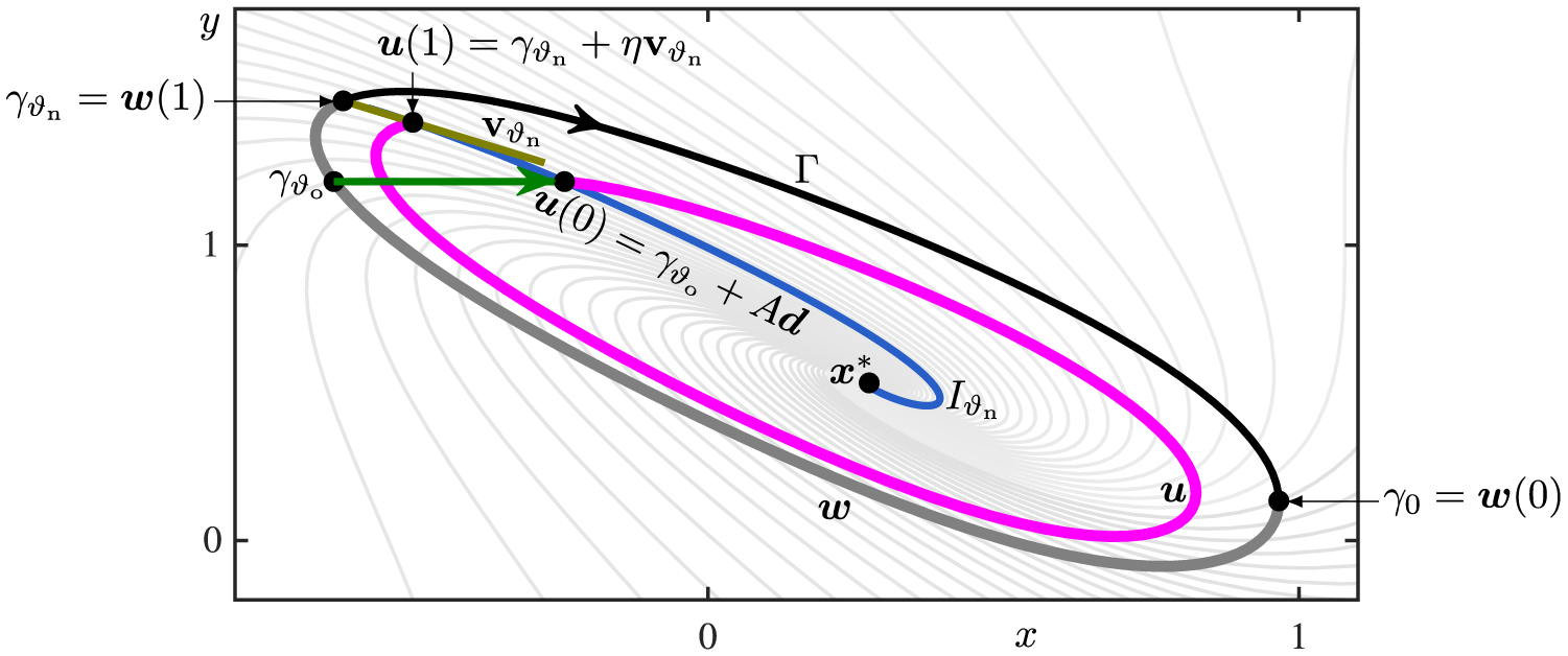
The orbit segment $\boldsymbol {u}$
is subject to the boundary conditions
$\boldsymbol {u}$
is subject to the boundary conditions
 $$ \begin{align} \boldsymbol{u}(0) & = \gamma_{\vartheta_{\mathrm{o}}} + A \, \boldsymbol{d}(\varphi_{\mathrm{d}}) = \gamma_{\vartheta_{\mathrm{o}}} + A \, [\cos{(\varphi_{\mathrm{d}})}, \sin{(\varphi_{\mathrm{d}})}], \end{align} $$
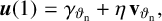 $$ \begin{align} \boldsymbol{u}(1) & = \gamma_{\vartheta_{\mathrm{n}}} + \eta \, \mathbf{v}_{\vartheta_{\mathrm{n}}},\qquad\qquad\qquad\ \ \qquad\qquad\qquad \end{align} $$
where $\mathbf {v}_{\vartheta _{\mathrm {n}}}$
is the stable unit Floquet vector at
$\mathbf {v}_{\vartheta _{\mathrm {n}}}$
is the stable unit Floquet vector at $\gamma _{\vartheta _{\mathrm {n}}} \in \Gamma $
and the distance
$\gamma _{\vartheta _{\mathrm {n}}} \in \Gamma $
and the distance $\eta \in \mathbb {R}$
from
$\eta \in \mathbb {R}$
from $\gamma _{\vartheta _{\mathrm {n}}}$
is small. While
$\gamma _{\vartheta _{\mathrm {n}}}$
is small. While $\gamma _{\vartheta _{\mathrm {o}}}$
is taken as input here, the point
$\gamma _{\vartheta _{\mathrm {o}}}$
is taken as input here, the point $\gamma _{\vartheta _{\mathrm {n}}}$
is given by its phase shift
$\gamma _{\vartheta _{\mathrm {n}}}$
is given by its phase shift $\vartheta _{\mathrm {n}}$
from
$\vartheta _{\mathrm {n}}$
from $\gamma _{0}$
, as determined by the auxiliary orbit segment
$\gamma _{0}$
, as determined by the auxiliary orbit segment $\boldsymbol {w}$
with
$\boldsymbol {w}$
with $\boldsymbol {w}(0) = \gamma _{0}$
and
$\boldsymbol {w}(0) = \gamma _{0}$
and $\boldsymbol {w}(1) = \gamma _{\vartheta _{\mathrm {n}}}$
; finding
$\boldsymbol {w}(1) = \gamma _{\vartheta _{\mathrm {n}}}$
; finding $\gamma _{\vartheta _{\mathrm {n}}}$
in this way also means that
$\gamma _{\vartheta _{\mathrm {n}}}$
in this way also means that $\mathbf {v}_{\vartheta _{\mathrm {n}}}$
is known; see [Reference Langfield, Krauskopf, Osinga, Junge, Schütze, Froyland, Ober-Blöbaum and Padberg-Gehle13] for further details.
$\mathbf {v}_{\vartheta _{\mathrm {n}}}$
is known; see [Reference Langfield, Krauskopf, Osinga, Junge, Schütze, Froyland, Ober-Blöbaum and Padberg-Gehle13] for further details.
When $\eta $
in (A.3) is sufficiently small,
$\eta $
in (A.3) is sufficiently small, $\boldsymbol {u}(1)$
lies on the isochron
$\boldsymbol {u}(1)$
lies on the isochron $I_{\vartheta _{\mathrm {n}}}$
to good approximation; this can be achieved by choosing K in (A.1) large enough. Since the integration time is a multiple of
$I_{\vartheta _{\mathrm {n}}}$
to good approximation; this can be achieved by choosing K in (A.1) large enough. Since the integration time is a multiple of $T_\Gamma $
, the point
$T_\Gamma $
, the point $\boldsymbol {u}(0)$
also lies on
$\boldsymbol {u}(0)$
also lies on $I_{\vartheta _{\mathrm {n}}}$
to good approximation. In Figure 12, we show the case
$I_{\vartheta _{\mathrm {n}}}$
to good approximation. In Figure 12, we show the case $K = 1$
with a rather large
$K = 1$
with a rather large $\eta $
for illustrative purposes; specifically, we have that
$\eta $
for illustrative purposes; specifically, we have that $\mathcal {P}_A(0.5) = 0.6$
for
$\mathcal {P}_A(0.5) = 0.6$
for $A \approx 0.3899$
.
$A \approx 0.3899$
.
The BVP (A.1)–(A.3) for $\boldsymbol {u}$
is very flexible and allows the computation of different kinds of objects of interest. The isochron
$\boldsymbol {u}$
is very flexible and allows the computation of different kinds of objects of interest. The isochron $I_{\vartheta _{\mathrm {n}}}$
(of a planar system) for fixed
$I_{\vartheta _{\mathrm {n}}}$
(of a planar system) for fixed $\vartheta _{\mathrm {n}}$
is traced out by
$\vartheta _{\mathrm {n}}$
is traced out by $\boldsymbol {u}(0)$
as an arclength parametrized curve by performing a continuation in
$\boldsymbol {u}(0)$
as an arclength parametrized curve by performing a continuation in $\eta $
; here, we ensure that
$\eta $
; here, we ensure that $\eta $
is always sufficiently small by increasing K as necessary [Reference Hannam, Krauskopf and Osinga9, Reference Langfield, Krauskopf and Osinga11, Reference Osinga and Moehlis16]. Moreover, when choosing
$\eta $
is always sufficiently small by increasing K as necessary [Reference Hannam, Krauskopf and Osinga9, Reference Langfield, Krauskopf and Osinga11, Reference Osinga and Moehlis16]. Moreover, when choosing $\vartheta _{\mathrm {o}}$
as the continuation parameter for fixed
$\vartheta _{\mathrm {o}}$
as the continuation parameter for fixed $\varphi _{\mathrm {d}}$
and A, one generates the PTC as the graph
$\varphi _{\mathrm {d}}$
and A, one generates the PTC as the graph $(\vartheta _{\mathrm {o}},\mathcal {P}_A(\vartheta _{\mathrm {o}}))$
. Finally, a phase-resetting surface can be constructed and rendered from a sequence of PTCs computed for a suitable set of values of either A or
$(\vartheta _{\mathrm {o}},\mathcal {P}_A(\vartheta _{\mathrm {o}}))$
. Finally, a phase-resetting surface can be constructed and rendered from a sequence of PTCs computed for a suitable set of values of either A or $\varphi _{\mathrm {d}}$
; it is also possible to construct it from curves at given “heights”, which can be found by fixing
$\varphi _{\mathrm {d}}$
; it is also possible to construct it from curves at given “heights”, which can be found by fixing $\vartheta _{\mathrm {n}}$
at a suitable set of values.
$\vartheta _{\mathrm {n}}$
at a suitable set of values.


 Open access