


1. Introduction
Gas evolution reactions play an important role in many electrochemical processes of interest. These reactions include hydrogen and oxygen evolution reactions in water-splitting electrolyzers, chlorine and hydrogen evolution reactions in the chloralkaline process, the  $\textrm {CO}_2$ reduction reaction for regenerating fuels and many others. The life cycle of a bubble at a gas-evolving electrode begins with the nucleation at a suitable site of the electrode surface of a cluster of gas molecules from a solution supersaturated with dissolved gas. The bubble grows by taking up dissolved gas that reaches its surface by diffusion (Brandon & Kelsall Reference Brandon and Kelsall1985; Enríquez et al. Reference Enríquez, Sun, Lohse, Prosperetti and van der Meer2014), and detaches from the electrode when the buoyancy force, aided by hydrodynamic forces if the liquid flows around the electrode (Eigeldinger & Vogt Reference Eigeldinger and Vogt2000), overcomes the surface tension and electric forces that keep the bubble on the electrode surface (Brandon et al. Reference Brandon, Kelsall, Levine and Smith1985; Oguz & Prosperetti Reference Oguz and Prosperetti1993; Lv et al. Reference Lv, Le The, Eijkel, van den Berg, Zhang and Lohse2017). The detached bubble then drifts in the liquid until it reaches the surface where the gas is collected. Coalescence of bubbles may occur before and after detachment.
Bubbles affect the electrochemical reactions at the electrode in various ways. On the one hand, attached bubbles cover a fraction of the electrode surface, which reduces the wet surface where reactions occur and hinders the transport of mass and electric charge between the electrode and the liquid. On the other hand, the bubbles are sinks of dissolved gas, whose concentration decreases around them. Since the dissolved gas is the reaction product, its decrease leads to a decrease of the rate of the backward reaction and thus enhances gas evolution, opposing the effect of bubble coverage. The local density of electric current passing between the electrode and the liquid is proportional to the local rate of the electrochemical gas-evolving reaction, which in turn depends on the local concentrations of reactants and products at the electrode and increases with the applied voltage (see next section). To keep a given average current density in the presence of attached bubbles, the reaction rate in the part of the electrode not covered by bubbles must be higher than it was in the absence of bubbles. The variation of the applied voltage needed to achieve this goal, or the variation of the average current density if the voltage is kept constant, depends on which of the two effects dominates. Bubble coverage of the electrode tends to increase the required voltage, while bubble-induced decrease of the dissolved gas concentration tends to decrease it.
Correlating experimental data, Vogt & Balzer (Reference Vogt and Balzer2005) found that the bubble coverage increases nearly as the power 0.3 of the surface-averaged current density. The effects on bubble coverage of the electrode surface orientation and wettability, the composition and velocity of the electrolyte, the bubble departure radius, the temperature and the pressure have been investigated by a number of authors, and Vogt (Reference Vogt2017) put forward comprehensive scaling laws. The effect of attached bubbles on the electric resistance of the liquid was analysed by Sides & Tobias (Reference Sides and Tobias1980, Reference Sides and Tobias1982). The coupling of the two effects mentioned above with the transport of dissolved gas has been much studied (Vogt Reference Vogt1978, Reference Vogt1990; Dukovic & Tobias Reference Dukovic and Tobias1987; Leistra & Sides Reference Leistra and Sides1987; Gabrielli et al. Reference Gabrielli, Huet, Keddam, Macias and Sahar1989; Gabrielli, Huet & Nogueira Reference Gabrielli, Huet and Nogueira2005). The additional electric resistance of the liquid due to detached bubbles has been studied using well-known models of the conductivity of a liquid with dispersed bubbles together with models of the bubble distribution in the liquid. Detached bubbles also affect the transport of reactants and products of the electrochemical reaction.
In this paper, a simple model of the evolution of hydrogen at a cathode during the electrolysis of water is used to numerically analyse some of the issues mentioned above. A dilute aqueous solution undergoes a reduction reaction generating hydrogen at a horizontal cathode at the bottom of the liquid. The reaction rate is given by the Butler–Volmer model. The liquid is quiescent, except for the displacement imposed by the growth of the bubbles, and the transport of species in the liquid is due to diffusion and migration only. A layer of liquid on the cathode is simulated, which is limited above by a plane parallel to the cathode where the voltage relative to the cathode and the concentrations of all the species are constant. The growth of a single bubble attached to the cathode is computed using conditions of symmetry at some distance from the bubble to approximately account for the effect of other bubbles growing with a given spacing on the electrode. Alkaline and acidic solutions are considered, with and without a supporting electrolyte. The growth of the bubble is slow due to the low concentration of electroactive species and to the absence of liquid flow; the bubble is assumed to follow a sequence of equilibrium states, and the distributions of species concentrations and electric potential around the bubble are quasi-stationary. The electric current density averaged over the electrode surface and over the time of growth of the bubble is computed as a function of the voltage applied between the upper boundary and the electrode of the simulated half-cell. This current density is found to increase with the voltage and, for a given voltage, it is larger than the current density in the absence of bubbles. The result shows that the effect on the reaction rate of the decrease of supersaturation around the bubbles dominates the effect of the decrease of the active electrode area. The variation of the electrode potential due to both effects, and the voltage drop across the liquid, are analysed. The variation of the bubble spacing with applied voltage that leads to a constant maximum supersaturation on the electrode, which is the model prediction of bubble coverage, is computed.
2. Model formulation
2.1. Electrode reactions
Water electrolysis in an alkaline solution occurs through the global electrochemical reaction  $2 \textrm {H}_2\textrm {O} + 2 e^- \leftrightharpoons \textrm {H}_2 + 2 \textrm {OH}^-$ at the cathode of an electrolytic cell, and $2 \textrm {OH}^- \leftrightharpoons \frac {1}{2} \textrm {O}_2 + \textrm {H}_2\textrm {O} + 2 e^-$ at the anode. The cathode reaction includes reduction of water molecules with adsorption of hydrogen, $\textrm {M} + \textrm {H}_2\textrm {O} + e^- \leftrightharpoons \textrm {MH}_{ads} + \textrm {OH}^-$ (Volmer), where $\textrm {M}$ denotes free sites at the electrode and $\textrm {MH}_{ads}$ sites occupied by an adsorbed hydrogen atom, followed by either or both of electrochemical hydrogen desorption, $\textrm {MH}_{ads} + \textrm {H}_2\textrm {O} + e^- \leftrightharpoons \textrm {M} + \textrm {H}_2 + \textrm {OH}^-$ (Heyrovsky) and chemical desorption, $2 \textrm {MH}_{ads} \leftrightharpoons 2 \textrm {M} + \textrm {H}_2$ (Tafel). The hydroxide ions generated at the cathode travel to the anode where the oxidation reaction mentioned above occurs through a complex scheme, generating oxygen and recovering half of the water consumed at the cathode.
In an acidic solution, water decomposes at the anode in the oxidation reaction  $\textrm {H}_2\textrm {O} \leftrightharpoons \frac {1}{2} \textrm {O}_2 + 2 \textrm {H}^+ + 2 e^-$. The protons travel to the cathode (as hydronium ions $\textrm {H}_3\textrm {O}^+$) where they are reduced in the reaction $2 \textrm {H}^+ + 2 e^- \leftrightharpoons \textrm {H}_2$, which includes the stage $\textrm {M} + \textrm {H}^+ + e^- \leftrightharpoons \textrm {MH}_{ads}$ followed by $\textrm {MH}_{ads} + \textrm {M} + \textrm {H}^+ + e^- \leftrightharpoons 2 \textrm {M} + \textrm {H}_2$ and/or $2 \textrm {MH}_{ads} \leftrightharpoons 2 \textrm {M} + \textrm {H}_2$.
Alkaline water-splitting electrolyzers are a well-established technology. Most commonly, the water contains a high concentration of  $\textrm {KOH}$ that displaces the $\textrm {H}^+$– $\textrm {OH}^-$ equilibrium toward increasing the concentration of $\textrm {OH}^-$ and increases the conductivity of the liquid. The solutions around the electrodes are separated by a membrane that lets pass $\textrm {OH}^-$ but not other ions. An acidic solution can be prepared by dissolving a strong acid such as $\textrm {SO}_4\textrm {H}_2$ in water. This, however, is not used in industrial applications. Existing acidic electrolyzers feature a proton exchange membrane instead of a liquid electrolyte.
The electrode reactions mentioned above are not elementary processes. Each occurs through a kinetic scheme that includes adsorption, several electron transfer reactions and desorption. These elementary processes occur in thin non-neutral double layers on each electrode surface and depend on the material and structure of the surface. A double layer includes the excess or defect of electrons at the electrode surface; the compact Stern layer containing molecules of the solvent and, sometimes, of specifically adsorbed neutral or ionic species, at distances from the electrode of the order of their size; and the diffuse Gouy–Chapman layer where solvated ions are non-specifically adsorbed at distances from the electrode of the order of their size or larger. The net charge in the double layer is null. The thickness of the diffusive layer is determined by the balance of the electric and thermal energies of the ions. For a 1:1 electrolyte, this thickness is  $( {\epsilon _0 \epsilon R T/2 n_0 F^2} )^{1/2}$, where $n_0$ is the molar concentration of both ionic species outside the layer, $\epsilon _0$ and $\epsilon$ are the permittivity of vacuum and the dielectric constant of the liquid, $R$ and $F$ are the universal gas constant and the Faraday constant (product of the electron charge and the Avogadro number) and $T$ is the temperature of the liquid. In water at 300 K, for $n_0=0.1$ mol l $^{-1}$, this thickness is approximately $10^{-9}$ m. The characteristic variation of the electric potential across the double layer is $R T/F = 30$ mV at 300 K.
In this work, attention will be confined to the hydrogen evolution occurring at a cathode, and the Butler–Volmer model will be used for the overall cathode reaction. In its simplest form, this model gives the rate  $\omega$ of the reaction (moles of hydrogen produced per unit electrode area per unit time) in terms of the local concentrations of the species at the cathode (but outside the double layer) and the local variation of electric potential across the double layer. In what follows, the expression ‘values at the cathode surface’ is understood to refer to the values of the variables immediately outside the double layer. Choosing the zero of the electric potential at the cathode and calling $\phi _0$ the potential immediately outside the double layer, the rate of the cathode reaction is taken to be
 \begin{equation} \omega = A_f\ \textrm{e}^{{-}E_f/R T} \ \textrm{e}^{\alpha_f F \phi_0/R T} n_{H_2O}^2 - A_b \ \textrm{e}^{{-}E_b/R T} \ \textrm{e}^{-\alpha_b F \phi_0/R T} n_{OH}^2 n_{H_2} \end{equation}
for an alkaline solution, and
 \begin{equation} \omega= A_f \ \textrm{e}^{{-}E_f/R T} \ \textrm{e}^{\alpha_f F \phi_0/R T} n_{H}^2 - A_b \ \textrm{e}^{{-}E_b/R T} \ \textrm{e}^{-\alpha_b F \phi_0/R T} n_{H_2} \end{equation}
for an acidic solution.
Here,  $n_j$ with $j=\textrm {H}_2\textrm {O}$, $\textrm {OH}$, $\textrm {H}$, $\textrm {H}_2$ are the molar concentrations of the water, hydroxide ions, protons and hydrogen, $A_f$ and $A_b$ are the pre-exponential factors for the forward and backward reactions, $E_f$ and $E_b$ are their activation energies and $\alpha _f$ and $\alpha _b$ are the so-called transfer coefficients, which must satisfy the condition $\alpha _f + \alpha _b=2$ to ensure that (2.1) or (2.2) reduces to the Nernst equilibrium relation when $\omega =0$.
The dependence of the reaction rate on the variation of electric potential across the double layer is the defining feature of electrochemical reactions. It reflects the effect of this difference of potential on the energy of the electrons at the cathode, and thus on the rate of the reactions in which an electron is transferred between the cathode and some species in the solution.
For given values of the concentrations of the species, the reaction will be in equilibrium (equal rates of the forward and backward reactions) when  $\phi _0$ has the value
 \begin{equation} \phi_0^{eq}= \frac{R T}{2 F} \ln \frac{A_b}{A_f} + \frac{E_f - E_b}{2 F} + \frac{R T}{2 F} \ln \frac{n_{OH}^2 n_{H_2}}{n_{H_2O}^2}, \end{equation}
or
 \begin{equation} \phi_0^{eq}= \frac{R T}{2 F} \ln \frac{A_b}{A_f} + \frac{E_f - E_b}{2 F} + \frac{R T}{2 F} \ln \frac{n_{H_2}}{n_{H}^2}, \end{equation}
for alkaline or acidic solutions, respectively. Since the concentrations change from point to point on the electrode and with time, it is convenient to introduce a reference state with selected values of the concentrations. The standard reference state is conventionally defined with the condition that the molar concentrations of the electroactive species be  $n^s=1$ mol l $^{-1}$ and that of water $n_w=55.55$ mol l $^{-1}$ (pure water); see, e.g. Bard & Faulkner (Reference Bard and Faulkner2001). Using a superscript $s$ to denote standard conditions, the equilibrium value of $\phi _0$ can be written as
 \begin{equation} \phi_0^{eq}=\phi_0^{eqs} + \frac{R T}{2 F} \ln \left( { \frac{n_w^2}{n^{s^3}} \frac{n_{OH}^2 n_{H_2}}{n_{H_2O}^2} } \right), \end{equation}
with
 \begin{equation} \phi_0^{eqs}= \frac{R T}{2 F} \ln \left( { \frac{A_b}{A_f} \frac{n^{s^3}}{n_w^2} } \right) + \frac{E_f-E_b}{2 F} \end{equation}
in the alkaline case, and
 \begin{equation} \phi_0^{eq}=\phi_0^{eqs} + \frac{R T}{2 F} \ln \frac{n^s n_{H_2}}{n_{H}^2}\\ \end{equation}
with
 \begin{equation} \phi_0^{eqs}= \frac{R T}{2 F} \ln \frac{A_b}{A_f n^s} + \frac{E_f-E_b}{2 F} \end{equation}
in the acidic case.
The electric current flowing per unit electrode area when the reaction occurs is  $i=2 F \omega$, the factor 2 reflecting that two electrons are needed to form a molecule of hydrogen. Separating the contributions of the forward and backward reactions, the current density can be written as $i=i_f-i_b$. In equilibrium, $i_f=i_b$, and the common value is named the exchange current, $i_0$. In the standard state,
 \begin{equation} i_0^s= 2 F A_f \ \textrm{e}^{{-}E_f/R T} \ \textrm{e}^{\alpha_f F \phi_0^{eqs}/R T} n_w^2 = 2 F A_b \ \textrm{e}^{{-}E_b/R T} \ \textrm{e}^{-\alpha_b F \phi_0^{eqs}/ R T} n^{s^3} ,\end{equation}
in the alkaline case and
 \begin{equation} i_0^s= 2 F A_f \ \textrm{e}^{{-}E_f/R T} \ \textrm{e}^{\alpha_f F \phi_0^{eqs}/R T} n^{s^2} = 2 F A_b \ \textrm{e}^{{-}E_b/R T} \ \textrm{e}^{-\alpha_b F \phi_0^{eqs}/ R T} n^s, \end{equation}
in the acidic case.
Both  $\phi _0^{eqs}$ and $i_0^s$ depend only on the electrode material and structure and on the temperature (and on the arbitrary choice of the concentrations in the standard state). The values of $A_f \ \textrm{e}^{-E_f/R T}$ and $A_b \ \textrm{e}^{-E_b/R T}$ can be written in terms of $\phi _0^{eqs}$ and $i_0^s$. Carrying them to the expression of the reaction rate, we obtain
 \begin{align} \omega&= \frac{i_o^s}{2 F} \left[ \exp({\alpha_f F (\phi_0-\phi_0^{eqs})/R T}) \left( {\frac{n_{H_2O}}{n_w} } \right)^2\right.\nonumber\\ &\quad \left. - \exp({-\alpha_b F (\phi_0-\phi_0^{eqs})/R T}) \left( {\frac{n_{OH}}{n^s} }\right)^2 \frac{n_{H_2}}{n^s} \right] \end{align}
in the alkaline case, and
 \begin{equation} \omega= \frac{i_o^s}{2 F} \left[ { \exp({\alpha_f F (\phi_0-\phi_0^{eqs})/R T}) \left( {\frac{n_{H}}{n^s} } \right)^2 - \exp({-\alpha_b F (\phi_0-\phi_0^{eqs})/R T}) \frac{n_{H_2}}{n^s} }\right] \end{equation}
in the acidic case.
It is worth noticing that increasing  $n_{OH}$ increases the rate of the backward reaction (the second term of (2.8)) in the alkaline case, while increasing $n_{H}$ increases the rate of the forward reaction (2.9) in the acidic case.
2.2. Conservation equations and electrode balances
As was mentioned before, this work focuses on the evolution of hydrogen bubbles at a cathode under the simplest possible conditions. Figure 1 is a sketch of the proposed model. The surface of the cathode is a horizontal plane,  $x=0$, at the bottom of the liquid. The bubbles attached to the cathode grow due to the diffusion flux of dissolved hydrogen reaching their surfaces. This diffusion flux is small because the concentrations of electroactive species in the liquid are assumed to be small, so that the bubbles follow a sequence of equilibrium shapes under the action of the gravity; see § 2.4 for details. The liquid around the bubbles is quiescent except for the slow motion imposed by the growth of the bubbles. To simplify the numerical computations, the unit cell of the two-dimensional array of attached bubbles is replaced by a circular cylinder, which makes the problem axisymmetric. The processes occurring at the cathode are approximately decoupled from the rest of the electrolytic cell by using the following assumption. The molar concentration of $\textrm {OH}^-$ (in the alkaline case) or of $\textrm {H}^+$ (in the acidic case), as well as the molar concentration of dissolved hydrogen and the electric potential relative to the cathode all take constant values at a certain distance $L$ above the cathode. Namely, $n_{OH}=n_r$ or $n_{H}=n_r$ and $n_{H_2}=n_{H_{2r}}$, $\phi =V$ at $x=L$, with $n_r$, $n_{H_{2r}}$ and $V$ constant, and $n_{H_{2r}} \leq n_s$, where $n_s$ is the saturation concentration of hydrogen in water. These conditions can be approximately realized if the cathode is at the base of a recess of depth $L$ and a stream of electrolyte flows horizontally above the recess that makes the composition of the liquid outside the recess uniform without inducing a significant flow inside. The anode (not represented in figure 1) is a horizontal electrode much larger than the cathode and located at a certain height above the recess, so that it acts as a non-polarizable electrode.

Figure 1. Definition sketch.
The condition that the concentrations of the electroactive species are small allows an additional simplification because the activities of these species can be taken to be equal to their concentrations. This condition is not satisfied in industrial electrolyzers, but the simplifications it brings in are not expected to qualitatively change the character of the solution.
Two types of electrolytes are considered. In one of them, a single substance is dissolved in water which fully dissociates into two ionic species;  $\textrm {OH}^-$ and the cation replacing $\textrm {H}^+$ (for example $\textrm {K}^+$) in the case of an alkaline solution, and $\textrm {H}^+$ and the anion replacing $\textrm {OH}^-$ (for example $\textrm {SO}_4^{2-}$) in the case of an acidic solution. Calling $n_+$ and $n_-$ the molar concentrations of cations and anions, the conservation equations for these species in the absence of liquid flow are
 \begin{equation} \frac{\partial n_{{\pm}}}{\partial t} + {\boldsymbol{\nabla}} \boldsymbol{\cdot} {\boldsymbol{j}}_{{\pm}} = 0 \quad \text{with} \enspace {\boldsymbol{j}}_{{\pm}}={\pm} n_{{\pm}} \kappa_{{\pm}} {\boldsymbol{E}} - D_{{\pm}} {\boldsymbol{\nabla}} n_{{\pm}} , \end{equation}
where  ${\boldsymbol {E}}=-{\boldsymbol {\nabla }} \phi$ is the electric field; $\kappa _{\pm }$ are the mobilities of the ions; and $D_{\pm }$ are their diffusivities, which satisfy $D_{\pm }=R T \kappa _{\pm }/|Z_{\pm }| F$, where $Z_{\pm }$ are the charge numbers of the ions. In the case of an alkaline solution, $Z_-=-1$ and $Z_+>0$ depends on the species dissolved in the liquid, while in the case of an acidic solution $Z_+=1$ and $Z_-<0$ depends on the species dissolved. In what follows, $Z$ will be used to denote $Z_+$ in the first case and $-Z_-$ in the second.
The solution is quasi-neutral outside the double layer on the electrode surface, so that the condition  $Z_+ n_+ + Z_- n_- = 0$ must be satisfied. Calling $n$ the common value of $Z_+ n_+$ and $-Z_- n_-$, the conservation equations can be linearly combined to give
 $$\begin{gather} {\boldsymbol{\nabla}} \boldsymbol{\cdot} [ { n (\kappa_+{+} \kappa_-) {\boldsymbol{E}} - (D_+{-} D_-) {\boldsymbol{\nabla}} n }] = 0 \end{gather}$$
 $$\begin{gather}\frac{\partial}{\partial t} (2 n) + {\boldsymbol{\nabla}} \boldsymbol{\cdot} [ { n (\kappa_+{-} \kappa_-) {\boldsymbol{E}} - (D_+{+} D_-) {\boldsymbol{\nabla}} n }] = 0 . \end{gather}$$
In quasi-stationary conditions, when the time derivative is negligible, these equations reduce to
 \begin{equation} \nabla^2 n = 0 \quad \text{and} \quad {\boldsymbol{\nabla}} \boldsymbol{\cdot} ( { n {\boldsymbol{\nabla}} \phi} ) = 0 . \end{equation}
Analogously, the conservation equation for dissolved hydrogen,  $\partial n_{H_2}/\partial t = D_{H_2} \nabla ^2 n_{H_2}$, where $D_{H_2}$ is the diffusivity of hydrogen in water, reduces to
 \begin{equation} \nabla^2 n_{H_2} = 0 . \end{equation}
At the edge of the double layer, in the part of the cathode surface not covered by bubbles, the balances of the fluxes of ions and dissolved hydrogen coming in or out of the double layer from/to the bulk of the liquid and the fluxes consumed or produced by the electrochemical reaction read
 \begin{equation} D_{{\mp}} \frac{\partial n}{\partial x} \mp n \kappa_{{\mp}} \frac{\partial \phi}{\partial x} ={\mp} 2 \omega , \quad D_{{\pm}} \frac{\partial n}{\partial x} \pm n \kappa_{{\pm}} \frac{\partial \phi}{\partial x} = 0 , \quad -D_{H_2} \frac{\partial n_{H_2}}{\partial x} = \omega , \end{equation}
where the upper signs are for the alkaline case and the lower signs for the acidic case. These balances can be rewritten as
 \begin{equation} \frac{\partial n}{\partial x} ={\mp} \frac{2 Z}{(1 + Z) D_{{\mp}}} \omega , \quad \frac{\partial n}{\partial x} \pm \frac{Z F}{R T} n \frac{\partial \phi}{\partial x} = 0 , \quad -D_{H_2} \frac{\partial n_{H_2}}{\partial x} = \omega. \end{equation}
These conditions, together with the condition  $\phi =\phi _0$, are imposed at $x=0$ neglecting the thickness of the double layer.
In the alkaline case, the distribution of  $n_{H_2O}$ on the electrode is needed to evaluate the reaction rate. Two different approximations will be used. One is to neglect water consumption setting $n_{H_2O}=n_w$ everywhere, which is justified for dilute solutions with $n_r \ll n_w$. Alternatively, water consumption may be approximately accounted for taking $n_{H_2O}=n_w$ at $x=L$ and assuming that water diffuses toward the electrode with a diffusion coefficient $D_{H_2O}$, which is taken to be the self-diffusion coefficient of water. Leaving out water evaporation, this approximation gives a linear relation between $n_{H_2O}$ and $n$ (see (2.29b) below).
The second type of electrolytic solution to be considered contains a high concentration of a supporting electrolyte in addition to the electroactive species. The supporting electrolyte does not take part in the electrode reactions but, owing to its high concentration, increases very much the electric conductivity of the solution. This decreases the electric field, so that the contribution of the migration to the flux of electroactive species (the first term of  ${\boldsymbol {j}}_{\pm }$ in (2.10)) can be neglected, and the electric potential throughout the solution is nearly equal to its value at the upper boundary $x=L$, where $\phi =V$.
In addition, the contribution of the electroactive species to the density of space charge is much smaller than that of the ions of the supporting electrolyte, so that the condition of quasi-neutrality is enforced essentially by the supporting electrolyte and does not impose an algebraic relation between the concentrations of the electroactive species. Under quasi-stationary conditions, the conservation equations of these species and of the dissolved hydrogen are  $\nabla ^2 n_+ = \nabla ^2 n_- = \nabla ^2 n_{H_2} = 0$. Moreover, since the flux of cations of the electroactive electrolyte reaching the cathode is null for an alkaline solution, the solution of the first of these equations with the idealized condition at $x=L$ is that $n_+$ is uniform, equal to its value at the upper boundary. Similarly, in the case of an acidic solution, the flux of anions is null at the cathode and the second conservation equation gives a uniform $n_-$ equal to its value at the upper boundary. Thus, only the distribution of one ionic species needs to be computed in each case. With the notation $n=n_-$ in the alkaline case and $n=n_+$ in the acidic case, the equations and boundary conditions at the electrode reduce to
 \begin{equation} \nabla^2 n = \nabla^2 n_{H_2}=0 , \quad x=0: D_{{\mp}} \frac{\partial n}{\partial x} ={\mp} 2 \omega , \quad -D_{H_2} \frac{\partial n_{H_2}}{\partial x} =\omega , \end{equation}
where, as before, the upper sign is for the alkaline case and the lower sign for the acidic case. The reaction rate is
 \begin{align} \omega&=\frac{i_0^s}{2 F} \left[ \exp({\alpha_f F (V - \phi_0^{eqs})/R T}) \left( {\frac{n_{H_2O}}{n_w} }\right)^2 \right.\nonumber\\ &\quad \left.- \exp({-\alpha_b F (V-\phi_0^{eqs})/R T}) \left( {\frac{n}{n^s} } \right)^2 \frac{n_{H_2}}{n^s} \right], \end{align}
in the alkaline case, and
 \begin{equation} \omega=\frac{i_0^s}{2 F} \left[ { \exp({\alpha_f F (V - \phi_0^{eqs})/R T}) \left( {\frac{n}{n^s} }\right)^2 - \exp({-\alpha_b F (V-\phi_0^{eqs})/R T}) \frac{n_{H_2}}{n^s} } \right], \end{equation}
in the acidic case.
The values of the diffusion coefficients of the different species are summarized in table 1.
Table 1. Diffusion coefficients at 300 K, in units of  $10^{-9}$ m $^2$ s $^{-1}$.
The remaining boundary conditions, completing the formulation of the problem, are the same for the two types of electrolytic solutions.
At the upper boundary,  $x=L$, the Dirichlet conditions $n=n_r$, $n_{H_2}=n_{H_{2r}}$, $\phi =V$ (and $n_{H_2O}=n_w$ in the alkaline case), are imposed, with $n_r$, $n_{H_{2r}}$, $V$ and $n_w$ constant.
2.3. Bubbles
The bubbles are assumed to contain hydrogen only, neglecting the evaporation of water and other species. If  $\varSigma _b$ denotes the surface of a bubble, with unit normal ${\boldsymbol {n}}_b$ pointing toward the liquid (see figure 1), the fluxes of electroactive species reaching this surface from the liquid must be zero, and the concentration of hydrogen at $\varSigma _b$ is given by the condition of local thermodynamic equilibrium. The first conditions read $D_{\pm } {\boldsymbol {n}}_b \boldsymbol {\cdot } {\boldsymbol {\nabla }} n_{\pm } \pm n_{\pm } \kappa _{\pm } {\boldsymbol {n}}_b \boldsymbol {\cdot } {\boldsymbol {\nabla }} \phi =0$, which can be combined to give ${\boldsymbol {n}}_b \boldsymbol {\cdot } {\boldsymbol {\nabla }} n = {\boldsymbol {n}}_b \boldsymbol {\cdot } {\boldsymbol {\nabla }} \phi = 0$. The equilibrium concentration of hydrogen at the liquid side of a planar interface is the saturation concentration at the temperature of the system, $n_s$, which is proportional to the pressure of the gas on the interface (Henry's law), being $n_s=7.8 \times 10^{-4}$ mol l $^{-1}$ at normal temperature and pressure. When the interface is not planar, the equilibrium concentration changes because the pressure of the gas is higher than the pressure of the liquid. The effect is small but it is taken into account by writing $n_{H_2}=n_s (1 + \delta p_g/p_0)$, where $p_0$ is the pressure of the liquid on the electrode and $\delta p_g$ is the excess of pressure of the hydrogen in the bubble above $p_0$.
The surface tension of the liquid ( $\sigma$) and its contact angle with the electrode ( $\theta$) are taken to be constant. Strictly, the surface tension depends on the variation of the electric potential across the double layer at the bubble surface and on the species adsorbed in this layer, which in turn depend on the local concentrations of the electrolyte and the conditions of operation. Similarly, the contact angle depends on the conditions of the double layer at the electrode surface (Bard & Faulkner Reference Bard and Faulkner2001). The constant values approximation is expected to be valid for dilute solutions.
The electric field inside the bubble is expected to be of the same order,  $V/L$, as in the liquid bulk when the electrode reaction is far from equilibrium. The net surface charge density and the electric stress at the bubble surface are then of orders $\epsilon _0 V/L$ and $\epsilon _0 V^2/L^2$, respectively, and the ratio of this stress to the surface tension stress is of order $\epsilon _0 V^2 \ell _c/\sigma L^2$. This is a small quantity, of the order of $10^{-10}$ when $V$ is of the order of one volt and $\ell _c \sim L$. The electric stress due to the net charge of the bubble surface does not affect the growth of the bubble.
The dipolar interaction of the double layers at the electrode and bubble surfaces, which depends on the pH of the solution and may have an effect on the bubble departure volume (Brandon et al. Reference Brandon, Kelsall, Levine and Smith1985; Yang et al. Reference Yang, Baczyzmalski, Cierka, Mutschke and Eckert2018) is left out here.
The bubble has a hydrostatic shape at any time, its volume increasing slowly at the rate at which dissolved hydrogen from the supersaturated liquid reaches its surface by diffusion, and detachment is assumed to occur when a hydrostatic solution ceases to exist. In terms of the capillary length  $\ell _c=( {\sigma /\rho g})^{1/2}$, where $\rho$ is the density the liquid and $g$ is the acceleration due to gravity, the volume of a bubble at detachment is $V_{b_d}=\ell _c^3 f_1(\theta )$, where $f_1$ is a known function. The excess of pressure of the gas in a bubble of volume $V_b \leq V_{b_d}$ above the pressure $p_0$ of the liquid at the base of the bubble is $\delta p_g=\rho g \ell _c f_2(V_b/\ell ^3, \theta )$, where the function $f_2$ is known (Bashforth & Adams Reference Bashforth and Adams1883; Hartland & Hartley Reference Hartland and Hartley1976; Chester Reference Chester1978; Longuet-Higgins, Kerman & Lunde Reference Longuet-Higgins, Kerman and Lunde1991). The mass of hydrogen reaching the surface of the bubble and vaporizing per unit time is $\dot {m}=W_{H_2} D_{H_2} \int _{\varSigma _b} { {\boldsymbol {n}}_b \boldsymbol {\cdot } {\boldsymbol {\nabla }} n_{H_2} \, \textrm {d} A}$, where $W_{H_2}$ is the molecular mass of hydrogen and the integral extends to the surface of the bubble in contact with the liquid, $\varSigma _b$.
The temperature is assumed to be constant during the growth of the bubble, and the density of each material element of gas in the bubble satisfies the equation of state  $\rho _g=W_{H_2} p_g/R T$. The hydrogen that vaporized in a time interval $\textrm {d} t'$ about a time $t'$, when the pressure in the bubble was $p_g(t')=p_0 + \delta p_g(t')$, occupied a volume $\textrm {d} V_b' = R T \dot {m}(t')\, \textrm {d} t'/[W_{H_2} p_g(t')]$ at that time. At a later time $t$, when the pressure in the bubble is $p_g(t)$, the volume occupied by this gas is $\textrm {d} V_b = \textrm {d} V_b' p_g(t')/p_g(t)=R T \dot {m}(t')\, \textrm {d} t'/[W_{H_2} p_g(t)]$, and the total volume of the bubble is
 \begin{equation} V_b(t)=V_{b_i} + \frac{R T}{W_{H_2} p_g(t)} \int_0^t {\dot{m}(t') \, \textrm{d} t'} , \end{equation}
where  $V_{b_i}$ is the initial volume of the bubble, when it begins to grow following nucleation. This result can be recast as
 \begin{equation} \frac{\textrm{d} V_b}{\textrm{d} t} = \frac{R T}{W_{H_2} p_g(t)} \dot{m}(t) - \frac{R T}{W_{H_2} p_g(t)^2} \int_0^t {\dot{m}(t') \, \textrm{d} t'} \frac{\textrm{d} p_g}{\textrm{d} t} , \end{equation}
where the first term on the right-hand side is the rate at which the volume of the bubble increases due to the instantaneous vaporization of hydrogen while the second term is the rate of change of the volume due to the expansion of the hydrogen that vaporized at earlier times.
In the simplified axisymmetric problem, a single bubble is assumed to grow around a point of the cathode surface. The effect of other bubbles growing on the cathode is approximately accounted for by using zero derivative conditions for all the variables at a given distance,  $W$, from the axis of the bubble (see figure 1). This models the synchronous growth of a two-dimensional array of equispaced bubbles.
No attempt is made to describe the nucleation of bubbles at the electrode surface. Instead, the growth of a bubble is computed from an initial state when its volume,  $V_{b_i}$, is small compared with the volume at detachment. In the simulations discussed below, the ratio of initial to final volume is 1/50, and the results are insensitive to the value of this ratio.
2.4. Dimensionless variables
Cylindrical coordinates  $(x, r)$ will be used, where $x$ is the distance to the cathode and $r$ is the distance to the symmetry axis of the central attached bubble (see figure 1). The surface of this bubble is denoted $f_b(x,r,t)=0$, and the radius of its contact circle with the cathode is $r_c(t)$.
For convenience, the electric potential relative to its equilibrium value in standard conditions,  $\tilde {\phi }=\phi -\phi _0^{eqs}$, will be used instead of $\phi$.
The problem can be written in dimensionless form scaling distances with the capillary length  $\ell _c=(\sigma /\rho g)^{1/2}$, the redefined potential $\tilde {\phi }$ with $R T/F$, the molar concentration of water with $n_w$ and those of other species with the concentration $n_r$ of $\textrm {OH}^-$ (in the alkaline case) or of $\textrm {H}^+$ (in the acidic case) at the upper boundary $x=L$. The electric current density $i$ is scaled with $F D_{OH} n_r/\ell _c$ in the alkaline case and with $F D_{H} n_r/\ell _c$ in the acidic case. In that follows, the dimensionless variables are denoted with the same symbols used before for their dimensional counterparts.
In terms of these variables, the problem in the absence of supporting electrolyte becomes
 \begin{equation} \nabla^2 n = 0 , \quad {\boldsymbol{\nabla}} \boldsymbol{\cdot} ( {n {\boldsymbol{\nabla}} \tilde{\phi}}) = 0 , \quad \nabla^2 n_{H_2} = 0 \end{equation}
with the boundary conditions
 $$\begin{gather} \frac{\partial n}{\partial x} ={\mp} \frac{2 Z}{1 + Z} \omega , \ \ \frac{\partial n}{\partial x} \pm Z n \frac{\partial \tilde{\phi}}{\partial x} = 0 ,\ \ -D_{H_2} \frac{\partial n_{H_2}}{\partial x} = \omega \ \ \text{at} \ x=0 , \ r_c < r< W \end{gather}$$
 $$\begin{gather}n=1 , \quad \tilde{\phi} = \tilde{V} , \quad n_{H_2} = n_{H_{2r}} \quad \text{at} \ x=L \end{gather}$$
 \begin{equation} {\boldsymbol{n}}_b \boldsymbol{\cdot} {\boldsymbol{\nabla}} n = {\boldsymbol{n}}_b \boldsymbol{\cdot} {\boldsymbol{\nabla}} \tilde{\phi} = 0 , \quad n_{H_2}=n_s \left( {1+ \frac{\delta p_g}{p_0} } \right) \quad \text{at} \enspace f_b(x,r,t)=0, \end{equation}
with
 \begin{gather} {\boldsymbol{n}}_b=\frac{{\boldsymbol{\nabla}} f_b}{|{\boldsymbol{\nabla}} f_b|} \end{gather}
 \begin{gather} \frac{\partial n}{\partial r} = \frac{\partial \tilde{\phi}}{\partial r} = \frac{\partial n_{H_2}}{\partial r} = 0 \quad \text{at} \ r=W \end{gather}
where
 $$\begin{gather} \omega = \textrm{Da} ( { \textrm{e}^{\alpha_f \tilde{\phi}} n_{H_2O}^2 - \varLambda \ \textrm{e}^{-\alpha_b \tilde{\phi}} n^2 n_{H_2} } ) \quad \text{in the alkaline case,} \end{gather}$$
 $$\begin{gather}\omega = \textrm{Da} ( { \textrm{e}^{\alpha_f \tilde{\phi}} n^2 - \varLambda \ \textrm{e}^{-\alpha_b \tilde{\phi}} n_{H_2} }) \quad \text{in the acidic case.} \end{gather}$$
Here,  $D_{H_2}$ is the diffusivity of hydrogen scaled with $D_{OH}$ in the alkaline case and with $D_{H}$ in the acidic case, $n_s$ is the saturation concentration of hydrogen at the pressure $p_0$ of the liquid on the electrode scaled with $n_r$, $\tilde {V}=F (V - \phi _0^{eqs})/R T$ is the dimensionless voltage at the upper boundary relative to the standard equilibrium potential $\phi _0^{eqs}$ and $-n_{bx}=\cos \theta$ at the contact line $r=r_c(t)$. The parameters in the expressions of the reaction rate are $\textrm {Da}=i_0^s \ell _c/(2 F D_{OH} n_r)$ and $\varLambda =(n_r/n^s)^3$ in the alkaline case, and $\textrm {Da}=i_0^s n_r \ell _c/(2 F D_{H} n^{s^2})$ and $\varLambda =n^s/n_r$ in the acidic case. In these dimensionless variables, $i = 2 \omega$.
In the alkaline case, the dimensionless concentration of water is
 \begin{equation} n_{H_2O} = 1 \quad \text{or} \quad n_{H_2O} = 1 - \frac{n_r}{n_w} \frac{1 + Z}{Z} \frac{n - 1}{D_{H_2O}} , \end{equation}
depending on whether water consumption is neglected or approximately taken into account. In the second case, the diffusivity of water,  $D_{H_2O}$, is scaled with $D_{OH}$.
The solution of the problem depends on the dimensionless parameters  $\textrm {Da}$, $\varLambda$, $\alpha _f$, $\tilde {V}$, $\theta$, $L$,
$L$,  $W$,
$W$,  $n_s$, $n_{H_{2r}}$ and $Z$, in addition to the hydrogen diffusivity scaled with $D_{OH}$ or $D_{H}$ and the diffusivity of water scaled with $D_{OH}$, if water consumption is taken into account. The parameter $\varLambda$ is a consequence of the arbitrary choice of the standard state concentrations. It would become unity if the standard state was defined as that with $n$ and $n_{H_2}$ equal to $n_r$ (in dimensional variables).
The dimensionless problem with a supporting electrolyte is
 $$\begin{gather} \nabla^2 n = \nabla^2 n_{H_2} = 0 \end{gather}$$
 $$\begin{gather}\frac{\partial n}{\partial x} ={\mp} 2 \omega , \quad -D_{H_2} \frac{\partial n_{H_2}}{\partial x} = \omega \quad \text{at} \ x=0 \end{gather}$$
 $$\begin{gather}n=1, \quad n_{H_2} = n_{H_{2r}} \quad \text{at} \ x=L \end{gather}$$
 $$\begin{gather}{\boldsymbol{n}}_b \boldsymbol{\cdot} {\boldsymbol{\nabla}} n = 0 , \quad n_{H_2}=n_s (1 + \delta p_g/p_0) \quad \text{at} \enspace f_b(x,r,t) = 0 \end{gather}$$
 $$\begin{gather}\frac{\partial n}{\partial r} = \frac{\partial n_{H_2}}{\partial r} = 0 \quad \text{at} \ r=W, \end{gather}$$
and  $\tilde {\phi }$ in the expression (2.27) or (2.28) of the reaction rate replaced by $\tilde {V}$.
In addition, in the alkaline case,
 \begin{equation} n_{H_2O} = 1 \quad \text{or} \quad n_{H_2O} = 1 - \frac{n_r}{n_w} \frac{n - 1}{D_{H_2O}} . \end{equation}
The quasi-stationary approximation used here may be marginally justified as follows. Returning for a moment to dimensional variables, the characteristic size of a bubble is  $\ell _c$, and the characteristic value of the mass of hydrogen reaching the bubble per unit time is, at most (see § 4.1 for a refined estimation), $\dot {m} \sim W_{H_2} D_{H_2} \Delta n_{H_2} \ell _c$, where $\Delta n_{H_2}$ is the difference between the maximum molar concentration of dissolved hydrogen (which is attained at the electrode, where hydrogen is generated) and the saturation concentration at the surface of the bubble, $n_s$. The characteristic time of growth of a bubble is therefore $t_b$ such that $\rho _g \ell _c^3/t_b \sim \dot {m}$, where $\rho _g=W_{H_2} p_g/R T \approx W_{H_2} p_0/R T$ is the characteristic density of the hydrogen in the bubble. Thus, $t_b/t_{dif} \sim p_0/(\Delta n_{H_2} R T)$ with $t_{dif}=\ell _c^2/D_{H_2}$. The factor $p_0/(\Delta n_{H_2} R T)$ depends on the supersaturation of the liquid. Calling $S$ the maximum value of the ratio $n_{H_2}/n_s$, we have $t_b/t_{dif} \sim p_0/[(S-1) n_s R T] \sim 51.395/(S-1)$ for $p_0=10^5$ Pa and $T=300$ K. This is fairly large for all but the highest values of the supersaturation expected, which justifies the quasi-stationary approximation in the region of size $\ell _c$ around the bubbles. In what follows, non-stationary effects are neglected in the whole domain $x < L$.
Even leaving out the factor  $p_0/(\Delta n_{H_2} R T)$, the diffusion time $t_{dif}$ is very large, of the order of 0.4 h. In practical applications, it is essential to speed up the growth of the bubbles by stirring the liquid. This has two effects. On the one hand, stirring leads to diffusion layers whose thickness may be small compared with the size of the bubbles, thus increasing the fluxes of electroactive species toward the electrode and the flux of dissolved hydrogen toward the bubbles. On the other hand, stirring reduces the size of the bubbles at detachment. If the evolution of the bubbles is sufficiently fast, detached bubbles are numerous and buoyancy induces a flow that enhances stirring. None of this, however, is taken into account in the model formulated here.
Turning back to dimensionless variables and scaling the time with  $(\ell _c^2/D_{H_2}) (p_0/n_r R T)$, the excess of pressure $\delta p_g$ with $p_0$ and the volume of the bubble with $\ell _c^3$, the time evolution equation for the volume of the bubble is
 \begin{equation} \frac{\textrm{d} V_b}{\textrm{d} t} = \frac{\dot{m}}{1+\delta p_g} - \frac{1}{(1+\delta p_g)^2} \frac{\textrm{d} \delta p_g}{\textrm{d} t} \int_0^t {\dot{m}(t') \, \textrm{d} t'}\quad \text{with} \ \dot{m}= \int_{\varSigma_b} {{\boldsymbol{n}}_b \boldsymbol{\cdot} {\boldsymbol{\nabla}} n_{H_2} \, \textrm{d} A} , \end{equation}
while the shape of the bubble is the equilibrium shape with volume  $V_b$.
The solution of the problem is computed stepwise. At a given time, for a certain shape of the bubble and its associated  $\delta p_g$, the distributions of $n$,
$n$,  $n_{H_2}$ and $\tilde {\phi }$ (in the case without supporting electrolyte) are determined by solving the stationary problem formulated above. This allows us to compute the evaporation rate $\dot {m}$ and thus update the bubble volume and its excess pressure $\delta p_g$.
The average current density on the electrode surface is
 \begin{equation} \bar{\imath}(t) = \frac{2 {\rm \pi}\int_{r_c}^W {2 \omega r \, \textrm{d} r}} {{\rm \pi} W^2} . \end{equation}
3. Stationary solution in the absence of bubbles
The distributions of the variables in the absence of bubbles depend only on the distance to the electrode.
Consider first the case without supporting electrolyte. For a given current density  $i$, the solution of (2.22)–(2.24) is
 \begin{equation} \left.\begin{gathered}
n = 1 \mp \frac{Z}{1+Z} i (x-L) , \\ \tilde{\phi}=\tilde{V}
\mp \frac{1}{Z} \ln \left[ { 1 \mp \frac{Z i}{1+Z}(x-L)
}\right] , \\ n_{H_2}=n_{H_{2r}} - \frac{i}{2 D_{H_2}}
(x-L) , \end{gathered}\right\}
\end{equation}
\begin{equation} \left.\begin{gathered}
n = 1 \mp \frac{Z}{1+Z} i (x-L) , \\ \tilde{\phi}=\tilde{V}
\mp \frac{1}{Z} \ln \left[ { 1 \mp \frac{Z i}{1+Z}(x-L)
}\right] , \\ n_{H_2}=n_{H_{2r}} - \frac{i}{2 D_{H_2}}
(x-L) , \end{gathered}\right\}
\end{equation}
where, again, the upper (lower) signs are for the alkaline (acidic) case. In particular, at  $x=0$, $n=1 \pm Z i L/(1+Z)$, $\tilde {\phi } \equiv \tilde {\phi }_0 = \tilde {V} \mp \ln [ {1 \pm Z i L/(1+Z) } ]/Z$ and $n_{H_2}=n_{H_{2r}} + i L/2 D_{H_2}$. (Notice that $\tilde {V}-\tilde {\phi }_0=\pm \ln [1 \pm Z i L/(1+Z)]/Z$ is not a linear function of the current density; Ohm's law in its usual form does not hold owing to the space variation of $n$.) Carrying these values and $n_{H_2O}$ from (2.29a,b) to (2.27) or (2.28), we find the current–voltage characteristic
 \begin{align} i& = 2 \textrm{Da} \left[ { \textrm{e}^{\alpha_f \tilde{V}} \left( {1+\frac{Z i L}{1+Z} }\right)^{-\alpha_f/Z} \left( {1-\frac{n_r}{n_w} \frac{i L}{D_{H_2O}} }\right)^2 } \right. \nonumber\\ &\quad \left. - \varLambda \ \textrm{e}^{-\alpha_b \tilde{V}} \left( {1+\frac{Z i L}{1+Z} }\right)^{2+\alpha_b/Z} \left( {n_{H_{2r}} + \frac{i L}{2 D_{H_2}} }\right) \right] \end{align}
in the alkaline case, and
 \begin{align} i &= 2 \textrm{Da} \left[ { \textrm{e}^{\alpha_f \tilde{V}} \left( {1-\frac{Z i L}{1+Z} }\right)^{2+\alpha_f/Z} } \right.\nonumber\\ &\quad \left. - \varLambda \ \textrm{e}^{-\alpha_b \tilde{V}} \left( {1-\frac{Z i L}{1+Z} }\right)^{-\alpha_b/Z} \left( {n_{H_{2r}} + \frac{i L}{2 D_{H_2}} }\right) \right] \end{align}
in the acidic case.
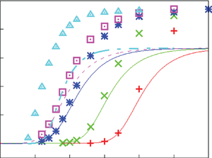
The results are shown in figure 2 for  $\alpha _f=\alpha _b=1$, $Z=1$, $L=6$, the values of the diffusivities in table 1 and various values of $\textrm {Da}$ and $\varLambda$, corresponding to the dimensional values $i_0^s=0.001$, 0.1, 10 A m $^{-2}$ and infinity, with $n_r=0.1$ (solid curves) and 0.5 mol l $^{-1}$ (dashed curves). In all the cases, the concentration of hydrogen at $x=L$ is $4 \times 10^{-4}$ mol l $^{-1}$, smaller than the saturation concentration $7.8 \times 10^{-4}$ mol l $^{-1}$. The curves in figure 2(a) show results for the alkaline case without accounting for water consumption (formally by letting $D_{H_2O} \rightarrow \infty$ in (3.2)). The uppermost curve in each figure shows results in the limit of infinitely fast, Nernstian reactions, $\textrm {Da} \rightarrow \infty$.

Figure 2. Dimensionless current density  $i$ as a function of the dimensionless voltage $\tilde {V}$ for alkaline (a) and acidic (b) solutions without supporting electrolyte. Solid curves are for $n_r=0.1$ mol l $^{-1}$ and dashed curves for $n_r=0.5$ mol l $^{-1}$. In each case, $i_0^s=10^{-3}$, 0.1, 10 A m $^{-2}$ and infinity, increasing from right to left. The inset in panel (a) shows the effect of water consumption. The horizontal asymptotes at the right-hand side of the inset are not realistic because the dilute solution approximation fails well before the reaction becomes diffusion limited. It is the effect of a moderate decrease of the water concentration at the cathode that is of interest in figure 5(a) below.
As can be seen, the dimensionless current density  $i$ increases with the exchange current (with $\textrm {Da}$ in dimensionless variables) in both cases. In the alkaline case, $i$ decreases when the concentration of the solution $n_r$, thus $n_{OH}$, is increased, because this decreases $\textrm {Da}$ and increases $\varLambda$ and the rate of the backward reaction. In the acidic case, $i$ increases with $n_r$, thus $n_{H}$, because now this increases $\textrm {Da}$ and decreases $\varLambda$. As noted at the end of § 2.1, $\textrm {OH}^-$ is a product of the electrolytic reaction in the alkaline case, while $\textrm {H}^+$ is a reactant in the acidic case.
In the acidic case, the asymptotic value of the current density for large  $\tilde {V}$ is the limiting current density $i_{L}=(1+Z)/(L Z)$ at which the concentration of $\textrm {H}^+$ at the electrode tends to zero. No limiting current density exists in the alkaline case if water consumption is neglected. Then the current density increases exponentially with the applied voltage, at a rate that increases with the dimensionless exchange current $\textrm {Da}$ and decreases when $\varLambda$ is increased. If water consumption is approximately taken into account, the current density increases less rapidly with $\tilde {V}$; see inset of figure 2(a). A saturation current density $i_{L}=D_{H_2O} n_w/(n_r L)$ is eventually approached in the inset at which $n_{H_2O}$ is zero at the electrode. However, the computation of this horizontal asymptote is not realistic because the dilute solution approximation would fail well before the concentration of water becomes small.
With a high concentration of a supporting electrolyte, the solution of (2.30)–(2.32) is
 \begin{equation} n=1 \mp i (x - L) , \quad n_{H_2} = n_{H_{2r}} - \frac{i}{2 D_{H_2}} (x - L) , \end{equation}
so that  $n=1 \pm i L$ and $n_{H_2} = n_{H_{2r}} + i L/2 D_{H_2}$ at $x=0$. Carrying this and $n_{H_2O}$ from (2.35a,b) to the expression of the reaction rate, we find
 \begin{equation} i = 2 \textrm{Da} \left[ { \textrm{e}^{\alpha_f \tilde{V}} \left( {1 - \frac{n_r}{n_w} \frac{i L}{D_{H_2O}} } \right)^2 - \varLambda \ \textrm{e}^{-\alpha_b \tilde{V}} (1 + i L)^2 \left( {n_{H_{2r}} + \frac{i L}{2 D_{H_2}} }\right) } \right] \end{equation}
in the alkaline case, and
 \begin{equation} i = 2 \textrm{Da} \left[ { \textrm{e}^{\alpha_f \tilde{V}} (1 - i L)^2 - \varLambda \ \textrm{e}^{-\alpha_b \tilde{V}} \left( {n_{H_{2r}} + \frac{i L}{2 D_{H_2}} }\right) } \right] \end{equation}
in the acidic case. Both are shown in figure 3 for the same values of the dimensionless parameters as in figure 2. (In the absence of water consumption in figure 3a).

Figure 3. Dimensionless current density  $i$ as a function of the dimensionless voltage $\tilde {V}$ for alkaline (a) and acidic (b) solutions with a high concentration of a supporting electrolyte. Solid curves are for $n_r=0.1$ mol l $^{-1}$ and dashed curves for $n_r=0.5$ mol l $^{-1}$. In each case, $i_0^s=10^{-3}$, 0.1 and 10 A m $^{-2}$, increasing from right to left.
The main quantitative difference with figure 2 occurs in the acidic case. The limiting current density is now  $i_{L}=1/L$, which for $Z=1$ is half the limiting current in figure 2. The concentration of $\textrm {H}^+$ decreases faster than before toward the electrode because the transport of cations is due only to diffusion, unaided by migration.
4. Results and discussion
4.1. Growth of a bubble
Figure 4(a) shows, for a few sample cases, the mass of hydrogen vaporizing per unit time as a function of the size of the bubble, defined as the cubic root of its volume, and figure 4(b) shows this size as a function of time. As can be seen, for the largest bubble spacing used ( $W=3$; dashed and dash-dot curves), the vaporization flux increases almost linearly with the size of the bubble and, after an initial stage, the size roughly approaches the $t^{1/2}$ law that is often assumed for diffusion controlled growth (Scriven Reference Scriven1959; Westerheide & Westwater Reference Westerheide and Westwater1961; Glas & Westwater Reference Glas and Westwater1964). The small departure from this law can be rationalized by noticing that the bubble grows in a region where the supersaturation is not uniform but decreases with the distance to the electrode. The diffusion flux reaching most of the bubble surface is of order $D_{H_2} \Delta n_{H_2} /V_b^{1/3}$, where, refining the estimation of § 2.4, $\Delta n_{H_2}$ is the difference between the concentrations of dissolved hydrogen far from the bubble but at distances to the electrode of order $V_b^{1/3}$ and at the surface of the bubble, where it is nearly $n_s$. Since the first concentration decreases as $V_b^{1/3}$ increases, the diffusion flux decays faster than $1/V_b^{1/3}$ and, accordingly, the size of the bubble increases less rapidly than the square root of time. A similar effect has been experimentally observed in the evaporation of a superheated liquid whose temperature decreases away from the wall where vapour bubbles grow; see Biasi, Stipari & Tozzi (Reference Biasi, Stipari and Tozzi1971). On the theoretical side, see the analysis of Cheh & Tobias (Reference Cheh and Tobias1968) for a hemispherical bubble growing on an electrode in a non-uniform concentration field, and the references therein.

Figure 4. (a) Mass of hydrogen vaporizing per unit time as a function of the cubic root of the bubble volume, and (b) cubic root of the bubble volume as a function of time, in linear and logarithmic scales (inset), for some sample cases. Solid: acidic,  $\tilde {V}=2$ and 5, $W=1$; dashed: acidic, $\tilde {V}=2$ and 5, $W=3$; dash-double-dot: alkaline, $\tilde {V}=-2$, $W=1$; dash-dot: alkaline, $\tilde {V}=-2$, $W=3$. For comparison, the dotted lines in (a) have slope 1, and the dotted lines at the lower part of (b) are $V_b^{1/3}=0.3 t^{1/2}$ and $V_b^{1/3}= 0.4 t^{1/3}$. Symbols in the log–log inset are experimental results of Brandon & Kelsall (Reference Brandon and Kelsall1985) for a Pt micro-electrode of 25 $\mathrm {\mu }$m diameter at two values of the electrode current, 10 $\mathrm {\mu }$A (up triangles) and 20 $\mathrm {\mu }$A (down triangles), with the time and the bubble volume multiplied by arbitrary factors.
For smaller bubble spacing ( $W=1$; solid and dash-double-dot curves in figure 4), the vaporization flux is nearly constant and the size of the bubble seems to approach a $t^{1/3}$ law during the last stages of the growth. This power law corresponds to the so-called direct injection regime (see, e.g. Verhaart, de Jonge & van Stralen Reference Verhaart, de Jonge and van Stralen1980; Brandon & Kelsall Reference Brandon and Kelsall1985), in which all the hydrogen generated at the electrode gets into the bubble. This is typical of micro- or nano-electrodes, in which the size of the bubble is large compared with the size of the electrode during much of the bubble growth. Then hydrogen is generated only around the base of the bubble, where a steep concentration gradient develops that drives the dissolved hydrogen toward the bubble. In the configuration at hand, with a large electrode and many attached bubbles, this regime can be approached when the bubbles are closely spaced, leaving only small interbubble gaps for the hydrogen to escape.
Symbols in figure 4(b) are experimental results of Brandon & Kelsall (Reference Brandon and Kelsall1985) for a micro-electrode of 25  $\mathrm {\mu }$m diameter and two values of the electrode current. In these experiments, the conditions of the bubble (which is anchored close to the periphery of the micro-electrode) and the surrounding electrolyte are quite different from those for an infinite electrode, leading to different values of the growth time and the final volume of the bubble. These magnitudes have been multiplied by arbitrary factors to fit them in figure 4(b), but the result still shows that, after an initial stage of fast growth, the time variation of the bubble size approaches a $t^{1/3}$ law.
Van der Linde et al. (Reference Van der Linde, Moreno-Soto, Peñas-López, Rodríguez-Rodríguez, Lohse, Gardeniers, van der Meer and Fernández-Rivas2017, Reference Van der Linde, Peñas-López, Moreno-Soto, van der Meer, Lohse, Gardeniers and Fernández-Rivas2018) devised an experiment allowing controlled nucleation and growth of a sequence of millimetre sized bubbles at a nucleation site consisting of a hydrophobic pit at the top of a pillar microfabricated on a silicon electrode. The growth of each bubble follows a  $t^{1/2}$ law, but with a proportionality coefficient that changes from bubble to bubble in response to the time variation of the hydrogen concentration in the surrounding electrolyte. The authors analyse this variation in detail with a view to improve the efficiency of water-splitting cells by means of micro-structured surfaces. Relying on similar ideas, Peñas et al. (Reference Peñas, van der Linde, Vijselaar, van der Meer, Lohse, Huskens, Gardeniers, Modestino and Fernández2019) use an hydrophobic site to induce nucleation outside the electrode surface, which in their experiments in a ring surrounding the nucleation site, thereby avoiding electrode coverage. All these experiments were carried out at constant current rather than constant voltage, which prevent direct comparison with the results of figure 4 for large bubble spacing.
4.2. Current density
The dimensionless current density averaged on the electrode surface (2.37) is further averaged over the growth time of a bubble. The result,  $\langle {i} \rangle$, is shown in figures 5 and 6 as a function of the voltage $\tilde {V}$ for various values of $\textrm {Da}$ and $\varLambda$. Figure 5 shows results in the absence of a supporting electrolyte, and figure 6 is for the case of a high concentration of supporting electrolyte. The thin curves in these figures show the current density in the absence of bubbles, already presented in figures 2 and 3, and the symbols are numerical results. As can be seen, the average current density $\langle {i} \rangle$ nearly coincides with the current density in the absence of bubbles at small values of $\tilde {V}$, and increases faster than it when $\tilde {V}$ increases, reflecting that the presence of bubbles enhances the gas-evolving reaction. In the alkaline case, without water consumption effects (figures 5a and 6a) the effect of the bubbles is moderate. In the acidic cases (figures 5b and 6b) the effect is more pronounced and increases with the exchange current and with $n_r$.

Figure 5. Space- and time-averaged current density as a function of the voltage  $\tilde {V}$, for alkaline solutions (a) and acidic solutions (b), without supporting electrolyte. Shown are results for $W=1$, $\theta =45^\circ$, values of other parameters used in § 3, and $n_r=0.1$ mol l $^{-1}$, $i_0^s=10^{-3}$ A m $^{-2}$ (pluses), $n_r=0.1$ mol l $^{-1}$, $i_0^s=0.1$ A m $^{-2}$ (crosses), $n_r=0.1$ mol l $^{-1}$, $i_0^s=10$ A m $^{-2}$ (starts) and $n_r=0.5$ mol l $^{-1}$, $i_0^s=10$ A m $^{-2}$ (open squares). For comparison, the thin curves show the current density in the absence of bubbles for the same values of the parameters. Solid curves are for $n_r=0.1$ mol l $^{-1}$, with $i_0^s$ increasing from right to left, and the dashed curve is for $n_r=0.5$ mol l $^{-1}$, $i_0=10$ A m $^{-2}$. In addition, the filled squares and the chain curve in (a) are results for $n_r=0.5$ mol l $^{-1}$, $i_0^s=10$ A m $^{-2}$ taking water consumption into account and the triangles and the chain curve in (b) are results for $n_r=0.1$ mol l $^{-1}$, $i_0^s$ infinite.

Figure 6. Space- and time-averaged current density as a function of the voltage  $\tilde {V}$, for alkaline solutions (a) and acidic solutions (b), with a high concentration of a supporting electrolyte. Shown are results for $W=1$, $\theta =45^\circ$, values of other parameters used in § 3, and $n_r=0.1$ mol l $^{-1}$, $i_0^s=10^{-3}$ A m $^{-2}$ (pluses), $n_r=0.1$ mol l $^{-1}$, $i_0^s=0.1$ A m $^{-2}$ (crosses), $n_r=0.1$ mol l $^{-1}$, $i_0^s=10$ A m $^{-2}$ (starts) and $n_r=0.5$ mol l $^{-1}$, $i_0^s=10$ A m $^{-2}$ (open squares). For comparison, the thin curves show the current density in the absence of bubbles for the same values of the parameters. Solid curves are for $n_r=0.1$ mol l $^{-1}$, with $i_0^s$ increasing from right to left, and the dashed curve is for $n_r=0.5$ mol l $^{-1}$, $i_0^s=10$ A m $^{-2}$.
In the acidic case, a transport limited state is approached for large values of  $\tilde {V}$ in which the average current density tends to a value different from the limiting current density in the absence of bubbles. In this transport limited state, $n$ tends to zero in the region of the electrode not covered by bubbles. The limiting distribution of $n$ can be computed using this condition instead of the first condition (2.23) or (2.31). The limiting distribution of $n_{H_2}$ can then be computed replacing the third condition (2.23) or the second condition (2.31) by $D_{H_2} \partial n_{H_2}/\partial x= -[(1+Z)/2 Z] \partial n/\partial x$ or $D_{H_2} \partial n_{H_2} =-\frac {1}{2} \partial n/\partial x$ at $x=0$. Both limiting distributions are independent of kinetic parameters and depend only on the geometrical parameters $L$ and $W$ and on $n_{{H_{2r}}}$ and $n_s$. The electric potential in the case without supporting electrolyte can finally be determined using the second condition (2.23), which gives an electric field that diverges at the electrode. The transport limited current density averaged on the electrode and its time-averaged value are
 \begin{equation} \bar{\imath}_{L}(t) = \frac{1+Z}{Z} \frac{2 {\rm \pi}\displaystyle\int_{r_c}^W { {\partial n/\partial x} |_{x=0} r \,\textrm{d} r}}{{\rm \pi} W^2} \quad \text{and} \quad \langle {i} \rangle _{L} = \frac{1}{T_b} \int_0^{T_b} {\bar{\imath}_{L} \, \textrm{d} t} \end{equation}
(with the factor  $(1+Z)/Z$ removed in the case with supporting electrolyte). Here, $T_b$ is the growth time of a bubble, up to detachment. Despite the fact that ${\partial n/\partial x} |_{x=0}$ tends to zero at the contact line, the value of $\bar {\imath }(t)$, and thus of $\langle {i} \rangle$, is higher than $i_{L}$ in the absence of bubbles for the values of $L$ and $W$ considered. This is because ${\partial n/\partial x} |_{x=0}$ overshoots above its limiting value $1/L$ in the absence of bubbles. For example $\langle {i} \rangle _{L}=0.451$, 0.356 and 0.341 for $W=1$, 2 and 3, respectively, with $L=6$, $n_{{H_{2r}}}=4 \times 10^{-3}$, $n_s=7.8 \times 10^{-3}$ and $Z=1$ without supporting electrolyte. These values are to be compared with $i_{L}=1/3$ in the absence of bubbles.
4.3. Distributions of variables at the electrode
The most significant feature of the solution is perhaps the decrease of the concentration of dissolved hydrogen,  $n_{H_2}$, around each bubble. On the electrode surface, this concentration increases from a minimum value close to the saturation concentration at the contact line to a maximum at the points farthest from the bubbles. At the beginning of the growth process, the maximum concentration is approximately the hydrogen concentration in the absence of bubbles when the bubble spacing $W$ is large, and smaller than this value when the spacing is decreased. As the bubbles grow, the maximum hydrogen concentration decreases in all cases. The hydrogen concentration increases with the concentration of the solution, $n_r$, and with the applied voltage $\tilde {V}$. The bubble-induced decrease of $n_{H_2}$ enhances the gas-evolving reaction by decreasing the rate of the backward reaction.
The electric potential at the edge of the double layer,  $\tilde {\phi }_0$, is equal to the applied voltage $\tilde {V}$ when the liquid contains a high concentration of supporting electrolyte. In the absence of supporting electrolyte, $\tilde {\phi }_0$ has only small space variations on the electrode. During most of the growth time, it increases slightly with distance to the contact line. When the bubble spacing is small ( $W=1$ and below), the maximum $\tilde {\phi }_0$ changes with time from slightly smaller to slightly larger than its value without bubbles, while $\tilde {\phi }_0$ is everywhere smaller than without bubbles when $W$ is larger. The value of $\tilde {\phi }_0$ increases with $\tilde {V}$ and decreases slightly when $n_r$ is increased. The minimum value of $\tilde {\phi }_0$, at the contact line, decreases with time. Similarly, the concentration at the electrode of $\textrm {OH}^-$ (in the alkaline case) or $\textrm {H}^+$ (in the acidic case) is nearly uniform and close to its value without bubbles. It slightly decreases around the contact line, to a minimum that decreases with time, while its value far from the contact line is slightly larger than without bubbles when the bubble spacing is small, and slightly smaller than this value when the spacing is increased. The space variations of $\tilde {\phi }_0$ and $n$ on the electrode decrease with the exchange current ( $\textrm {Da}$ in dimensionless variables).
The distribution of current density on the electrode is a consequence of these features. At small and moderate voltages, the current density increases around the bubbles at early times, reflecting the decrease of hydrogen concentration. At these times, the current density far from the bubbles is close to the current density without bubbles when the bubble spacing is large, and above this value when the spacing is decreased. At later times, the current density increases far from the bubbles and tends to become more uniform, until the effect of the decrease of  $\tilde {\phi }_0$ around the contact line comes into play and decreases the current density in this region. The effect of the space variation of $\tilde {\phi }_0$ and $n$ appears earlier at higher voltages, decreasing the current density around the contact line, where it reaches a minimum. In addition, the current density decreases with time everywhere on the electrode.
The current density tends to become uniform in the part of the electrode not covered with bubbles when  $\textrm {Da}$ and $i$ itself are small. The result was obtained by Dukovic & Tobias (Reference Dukovic and Tobias1987) in the framework of a different model. It can be rationalized by noticing that $\tilde {\phi }_0$ diverges logarithmically when $\textrm {Da} \rightarrow \infty$, while the space variations of $\tilde {\phi }$ in the cell, and thus the variations of $\tilde {\phi }_0$ at the electrode, as well as the variations of the concentrations of the reactants, are all small, of order $i$.
$i$.
4.4. Overpotentials
When the electrode reaction is at equilibrium ( $\omega =0$), the concentrations of all the species are uniform at their values at the upper boundary $x=L$; i.e. $n=1$, $n_{H_2}=n_{{H_{2r}}}$, $n_{H_2O}=1$ in dimensionless variables. The value of $\tilde {\phi }_0$ is then $\tilde {\phi }_0^{eq}= \frac {1}{2} \ln \varLambda + \frac {1}{2} \ln n_{{H_{2r}}}$. The overpotential is the variation of $\tilde {\phi }_0$ about this equilibrium value when the reaction proceeds at a given non-zero rate. It can be decomposed into two parts. First, the transport of species to and from the electrode associated with the given rate of the reaction causes variations of the species concentrations at the electrode (at the edge of the double layer) relative to the values they had when the reaction was at equilibrium. The variation of $\tilde {\phi }_0$ needed for the reaction to be at equilibrium with the modified values of the concentrations at the electrode is the concentration overpotential $\delta \tilde {\phi }_{0_c}= \frac {1}{2} \ln n_{H_2}/n_{{H_{2r}}} + \ln n - \ln n_{H_2O}$ in the alkaline case, and $\delta \tilde {\phi }_{0_c}= \frac {1}{2} \ln n_{H_2}/n_{{H_{2r}}} - \ln n$ in the acidic case. In each case, $\delta \tilde {\phi }_{0_c}$ is the sum of contributions of the species taking part in the reaction. The additional variation of $\tilde {\phi }_0$ needed for the reaction to proceed at the given rate is the activation overpotential $\delta \tilde {\phi }_{0_a} = \tilde {\phi }_0 - \tilde {\phi }_0^{eq} - \delta \tilde {\phi }_{0_c}$, which is an increasing function of the reaction rate.
Bubbles are known to affect the reaction rate in various manners; see Zhao, Ren & Luo (Reference Zhao, Ren and Luo2019) for a recent review. On the one hand, since nucleation, the bubbles are sinks of dissolved hydrogen, and therefore decrease the supersaturation of the liquid surrounding them below the value it would have without bubbles. Since the rate of the backward reaction increases with the concentration of hydrogen at the electrode, the presence of bubbles decreases this rate and thus enhances the gas evolution reaction. This effect is reflected in a decrease of the first term of the concentration overpotential. On the other hand, the attached bubbles cover a fraction of the electrode surface, rendering it inactive for electrochemical reactions. To keep a given average current density, the rate of the reaction must increase in the active part of the electrode surface, thereby increasing the activation overpotential. The two effects oppose each other. The net variation they induce of the voltage required to keep a given current density, or of the current density at a given voltage, depends on which of them dominates. There are also other effects of the bubbles that cannot be described with the model used here because they depend on the presence of many detached bubbles in the liquid. One of these is the increase of the ohmic resistance of the liquid due to these bubbles (additional to the increase due to attached bubbles), and another is the contribution of detached bubbles to the stirring of the liquid, which enhances the transport of reactants and products.
In the presence of bubbles, the concentration and activation overpotentials are functions of the position on the electrode and of time during the growth of a bubble. Inspection of the numerical solutions shows that the variations of these overpotentials due to the bubbles are more pronounced around the contact line but do not vanish on the rest of the electrode for the bubble spacings considered. Values of the overpotentials averaged over the active area of the electrode and over time are shown in figures 7 and 8 as functions of the applied voltage for various values of the solution concentration and the exchange current ( $\varLambda$ and $\textrm {Da}$ in dimensionless variables). For comparison, thin curves show the overpotentials without bubbles. Results are shown for the alkaline case without accounting for water consumption (a,b,c) and for the acidic case (d,e,f) in the absence (figure 7) and in the presence (figure 8) of supporting electrolyte. The results are qualitatively similar in both figures.

Figure 7. Space- and time-averaged overpotentials as functions of the voltage  $\tilde {V}$. Left-hand side panels are for alkaline solutions and right-hand side panels are for acidic solutions, both without supporting electrolyte. Results are shown for $W=1$, $\theta =45^\circ$, the same values of other parameters as in § 3, and values of $\textrm {Da}$ and $\varLambda$ corresponding to $n_r=0.1$ mol l $^{-1}$, $i_0^s=0.1$ A m $^{-2}$ (a,d); $n_r=0.1$ mol l $^{-1}$, $i_0^s=10$ A m $^{-2}$ (b,e); and $n_r=0.5$ mol l $^{-1}$, $i_0^s=10$ A m $^{-2}$ (c,f). In each case, solid curves are the contribution of dissolved hydrogen to the concentration overpotential, dotted curves are the contribution of $\textrm {OH}^-$ or $\textrm {H}^+$ to the concentration overpotential, and dashed curves are the activation overpotential. Thin curves show these magnitudes in the absence of bubbles.

Figure 8. Space- and time-averaged overpotentials as functions of the voltage  $\tilde {V}$. Left-hand side panels are for alkaline solutions and right-hand side panels are for acidic solutions, both with a high concentration of a supporting electrolyte. Results are shown for the same values of the parameters as in figure 7.
As can be seen, the concentration overpotential due to the variation of the concentration of hydrogen (solid curves) is an increasing function of the voltage in the alkaline case, for which there is no limiting current density, and reaches a plateau in the acidic case when the current density approaches its maximum. In both cases, this part of the concentration overpotential decreases in the presence of bubbles. The part of the concentration overpotential due to the variation of the concentrations of  $\textrm {OH}^-$ or $\textrm {H}^+$ (dotted curves) tends to increase linearly with $\tilde {V}$ and is nearly independent of the presence of bubbles. Finally, the activation overpotential (dashed curves) is rather different in the two cases. In the alkaline case, it increases slightly with the applied voltage, reaches a shallow maximum and eventually tends to zero when $\tilde {V} \rightarrow \infty$. In the acidic case, $\delta \tilde {\phi }_{0a}$ increases linearly with the voltage, keeping this trend in the transport limited regime for high voltages. The activation overpotential increases in the presence of bubbles. In the alkaline case, the bubble-induced decrease of the concentration overpotential is close to the increase of the activation overpotential, so that $\tilde {\phi }_0$ is nearly the same with and without bubbles for a given current density. In the acidic case, the bubble-induced decrease of the concentration overpotential is larger than the bubble-induced increase of the activation overpotential, so that the bubbles decrease the value of $\tilde {\phi }_0$ for a given average current density, in line with the results in figures 5 and 6.
The linear increase of  $\delta \tilde {\phi }_{0c}$ with $\tilde {V}$ in the alkaline case reflects the exponential increase of the reaction rate, and thus of $n_{H_2}$ and $n$ at the electrode. The boundedness of $\delta \tilde {\phi }_{0a}$ reflects that the backward reaction is always important.
In the acidic case, the space- and time-averaged concentration of  $\textrm {H}^+$ at the electrode tends to zero linearly as $\langle {i} \rangle \rightarrow \langle {i} \rangle _{L}$, the potential $\tilde {\phi }_0$ diverges logarithmically to keep $2\textrm {Da} \, n^2 \exp (\alpha _f \tilde {\phi }_0) = O(\langle {i} \rangle _{L})$, and $\tilde {V}-\tilde {\phi }_0$ also diverges logarithmically. This accounts for the linear trends of $\delta \tilde {\phi }_{0a}$ and the part of $\delta \tilde {\phi }_{0c}$ due to $\textrm {H}^+$, because $\ln n \sim \tilde {\phi }_0 \sim -\ln (\langle {i} \rangle _{L} - \langle {i} \rangle ) \sim \tilde {V}$. These results are analogous to the results of § 3 without bubbles, with $\langle {i} \rangle _{L}$ playing the role of $i_{L}$. The similarity is not unexpected because the integrals of the vertical diffusion and migration fluxes of ions, $-\partial n/\partial x$ and $n E_x$, across horizontal planes spanning the liquid are conserved as in the absence of bubbles.
Figure 9 shows the potential drop across the cell as a function of the applied voltage for alkaline and acidic solutions without supporting electrolyte. This drop is not proportional to the current density. In the alkaline case, without accounting for water consumption, the linear trend for large  $\tilde {V}$ reflects the combination of a current density that increases exponentially with $\tilde {\phi }_0$ and a potential drop that is expected to increase as the logarithm of the current density (as in the absence of bubbles; see § 3). In the acidic case, the linear trend is accounted for by the estimations of the previous paragraph.

Figure 9. Mean potential drop across the cell for alkaline (a) and acidic (b) solutions, with  $n_r=0.1$ mol l $^{-1}$, $i_0^s=0.1$ A m $^{-2}$ (solid), $n_r=0.1$ mol l $^{-1}$, $i_0^s=10$ A m $^{-2}$ (dashed) and $n_r=0.5$ mol l $^{-1}$, $i_0^s=10$ A m $^{-2}$ (dotted). Parameters $\alpha _f$, $Z$,
$Z$,  $\theta$, $L$,
$L$,  $W$,
$W$,  $n_s$ and $n_{{H_{2r}}}$ have the same values as in § 3 and figure 5.
4.5. Constant maximum supersaturation
Up to now, the bubble spacing  $W$ has been taken to be a constant parameter of the problem. The maximum supersaturation, defined as $S=\max n_{H_2}/n_s$ at each instant of time, is attained at the points of the electrode farthest from the bubbles, and increases when the voltage is increased keeping $W$ constant. This is not realistic. The real maximum supersaturation at which bubbles appear is high and difficult to measure, but recent results using nanoelectrodes to avoid the complexity of multiple nucleation sites (German et al. Reference German, Edwards, Ren and White2018) suggest that it is independent of the voltage for a given dissolved gas. To approximately account for this fact in the framework of the present model, additional computations have been carried out in which $W$ is a function of the voltage such that the maximum supersaturation has a given, constant value at the beginning of the growth, when the volume of the bubble is 1/50 of its volume at detachment. The average current density computed in these conditions is shown in figure 10(a) as a function of the voltage for various values of $S$ in a case of acidic solution without supporting electrolyte. Figure 10(b) shows the variation of the spacing $W$ with the voltage.
The results show that infinitely spaced bubbles first appear when the voltage reaches a certain value that increases with the chosen maximum supersaturation, and the bubble spacing decreases when the voltage is increased above this value. For the three lower values of  $S$ in figure 10, the surfaces of neighbouring bubbles come into contact at the instant of detachment when the voltage reaches a critical value. This heralds coalescence of attached bubbles at higher voltages.

Figure 10. Space- and time-averaged current density  $\langle {i} \rangle$ (a) and bubble spacing $W$ (b) as functions of the voltage $\tilde {V}$ computed with the condition that the maximum supersaturation $S$ be constant at the beginning of the bubble growth. Results are shown for an acidic solution with $n_r=0.1$ mol l $^{-1}$, $i_0^s=10$ A m $^{-2}$ ( $\varLambda = 10$, $\textrm {Da}=4.96 \times 10^{-3}$) without supporting electrolyte, with $S=6.42$ (pluses), 15.64 (crosses), 33.75 (stars) and 93.18 (open squares), and for $n_r=0.1$ mol l $^{-1}$, $i_0^s=0.1$ A m $^{-2}$ ( $\varLambda =10$, $\textrm {Da}=4.96 \times 10^{-5}$), with $S=6.42$ (filled squares). The solid curve in (a) shows the current density in the absence of bubbles. Parameters $\alpha _f$, $Z$,
$Z$,  $\theta$, $L$,
$L$,  $n_s$ and $n_{{H_{2r}}}$ have the same values as in § 3 and figure 5.
The spacing  $W$ seems to level off with increasing voltage at the highest value of $S$ in figure 10, for which no coalescence appears in the range of voltages where a solution has been computed.
Finally, since quasi-hydrostatic bubbles follow a constant path of shapes and volumes up to detachment, the inverse of the square of  $W$ is proportional to the fraction of the electrode area covered by bubbles predicted by the model.
Apparently, the coalescence of attached bubbles drives the system into a mode in which upward gas jets rising from the electrode coexist with downward liquid columns falling onto it, and the hydrodynamic instability of this mode is connected to the transition between the mode of gas evolution discussed in this article (analogous to the pool mode of boiling heat transfer) and modes in which a gas film blankets the electrode (analogous to the film mode of boiling heat transfer). The electric current density attains a maximum at the voltage of this transition and falls rapidly when the voltage is further increased. Unfortunately these modes and transitions are beyond the scope of the quasi-hydrostatic approximation used here.
5. Conclusions
The evolution of hydrogen at a cathode has been analysed using the Butler–Volmer model to compute the rate of the electrochemical reaction around an attached hydrogen bubble that grows slowly on top of a horizontal electrode at the bottom of a dilute, aqueous electrolyte. The liquid is quiescent and is bounded above by a horizontal plane where the voltage and the concentrations of all the species are constant. Symmetry conditions are used to simulate the effect of other bubbles growing on the electrode.
When the spacing of the bubbles on the electrode is large compared with the size of a bubble at detachment, the total flux of hydrogen reaching a bubble increases nearly linearly with the size of the bubble, leading to a size that nearly follows the  $t^{1/2}$ law expected for diffusion growth in a uniformly supersaturated liquid. The decrease of the supersaturation with distance to the electrode is felt in the region where the bubble grows, causing a slight lag of the bubble size behind the $t^{1/2}$ law. When the bubble spacing decreases, the interbubble gaps become narrow and most of the hydrogen generated at the electrode gets into the bubbles. This leads to a bubble size that increases nearly as $t^{1/3}$ during the last stages of the growth.
For dilute alkaline solutions, when the consumption of water is ignored, the space- and time-averaged current density increases exponentially with voltage above its equilibrium value. The current density also increases with the exchange current of the reaction, and decreases when the concentration of  $\textrm {OH}^-$ increases, as this increases the rate of the backward reaction.
For acidic solutions, the average current density increases with the exchange current and with the concentration of  $\textrm {H}^+$. At high voltages, the current density tends to a transport limited value that decreases when the spacing of the bubbles increases (though this is not displayed in figures 5 and 6) and when a high concentration of a supporting electrolyte is added to the water.
In both cases, the average current density is higher than the current density in the absence of bubbles, showing that the bubble-induced decrease of the concentration overpotential overcomes the increase of the activation overpotential due to the partial coverage of the electrode surface with bubbles. The concentration and activations overpotentials, as well as the electric potential drop across the liquid, are discussed for alkaline and acidic solutions.
The bubble spacing must decrease with increasing voltage to keep the maximum supersaturation constant. Computations carried out in these conditions give an estimation of the voltage and current density at which coalescence of attached bubbles first occur.
Funding
This work has been supported by the Spanish Ministerio de Ciencia y Universidades through projects DPI2017-86547-C2-2-P and PID2020-115730GB-C22, and by the Red Nacional para el Desarrollo de la Microfluídica (MIFLUNET) through projects DPI2015-71901-REDT and RED2018-102829-T.
Declaration of interests
The author reports no conflict of interest.


 Open access