


1. Introduction
The development of a turbulent mixing layer from the Rayleigh–Taylor instability (Rayleigh 1882; Taylor Reference Taylor1950) and the Richtmyer–Meshkov instability (Richtmyer Reference Richtmyer1960; Meshkov Reference Meshkov1969) can be observed in a variety of contexts ranging from inertial confinement fusion (ICF) (Lindl et al. Reference Lindl, Amendt, Berger, Glendinning, Glenzer, Haan, Kauffman, Landen and Suter2004, Reference Lindl, Landen, Edwards and Moses2014), supernova explosions (Arnett Reference Arnett2000) and supersonic combustion (Yang, Chang & Bao Reference Yang, Chang and Bao2014). The Rayleigh–Taylor instability (RTI) occurs when a light fluid is accelerated into a heavy fluid with a perturbed interface between the two. The misalignment between the density and pressure gradients causes a continual baroclinic deposition of vorticity, amplifying the instability. The Richtmyer–Meshkov instability (RMI) is similar, however, the acceleration is taken in the impulsive limit, such as experienced from a shock wave. With a short/transient deposition of vorticity, the instability is unstable whether accelerated heavy-to-light or light-to-heavy. Both instabilities can cause degradation in the performance of ICF, where fusion is attained by compressing a pellet of fuel in an implosion indirectly or directly driven by lasers. The implosion profile of the pellet utilises multiple shocks to compress the fuel, but this amplifies any imperfections in the fuel–shell interface. As the pellet implodes, the ablation front is RT unstable during the acceleration phase, which can feed through to the fuel–shell interface. During the deceleration phase, the fuel–shell interface becomes unstable, further driving the growth of the interface perturbations and mixing cold pellet material into the hot core and degrading ICF performance. For more details on RTI and RMI, thorough reviews have been conducted in the works of Zhou (Reference Zhou2017a , Reference Zhoub ); Zhou et al. (Reference Zhou2021), Zhou (Reference Zhou2024), Zhou, Sadler & Hurricane (Reference Zhou, Sadler and Hurricane2025).
When the mode’s amplitude is much smaller than its wavelength, RMI and RTI are in the linear regime limit, with the modes evolving independently. For RMI, this corresponds to a linear growth rate, whilst RTI experiences exponential growth. As a mode continues to grow it will enter the nonlinear regime, experiencing decreased growth and secondary instabilities forming, such as the Kelvin–Helmholtz instability, causing the modes to roll-up and asymmetries in the mixing layer to form. The penetrating structures are labelled spikes for where the heavy fluid penetrates the lighter fluid, and bubbles where the light fluid is penetrating into the heavy. For sufficiently high Reynolds numbers, these structures will further breakdown, creating a self-similar turbulent mixing layer. The mixing layer width $h$
in the late time grows according to
$h$
in the late time grows according to $h\propto \mathcal{A}_t g t^2$
for RTI, where
$h\propto \mathcal{A}_t g t^2$
for RTI, where $\mathcal{A}_t=(\rho _2-\rho _1)/(\rho _2+\rho _1)$
is the Atwood number representing the density difference of the two fluids (
$\mathcal{A}_t=(\rho _2-\rho _1)/(\rho _2+\rho _1)$
is the Atwood number representing the density difference of the two fluids ( $\rho _1$
and
$\rho _1$
and $\rho _2$
), and
$\rho _2$
), and $g$
is the acceleration. The RMI mixing layer grows according to
$g$
is the acceleration. The RMI mixing layer grows according to $h\propto \tau ^\theta$
, where
$h\propto \tau ^\theta$
, where $\tau$
is an appropriately non-dimensionalised time and
$\tau$
is an appropriately non-dimensionalised time and $\theta$
is a sublinear power law. For narrowband initial conditions (
$\theta$
is a sublinear power law. For narrowband initial conditions ( $k_{max}/k_{min} \leqslant 2$
, where
$k_{max}/k_{min} \leqslant 2$
, where $k$
is the wavenumber of the interface perturbation spectrum) the observed power law falls within the theoretical bounds of 1/4 (Soulard & Griffond Reference Soulard and Griffond2022) and 1/3 (Elbaz & Shvarts Reference Elbaz and Shvarts2018). Broadband initial conditions are observed to produce larger power-law growth rates in comparison (Thornber et al. Reference Thornber, Drikakis, Youngs and Williams2010; Groom & Thornber Reference Groom and Thornber2020). The bubble and spike heights for RMI are considered to grow according to the same power laws when analysed over a long enough period of time (Youngs & Thornber Reference Youngs and Thornber2020a
; Groom & Thornber Reference Groom and Thornber2023).
$k$
is the wavenumber of the interface perturbation spectrum) the observed power law falls within the theoretical bounds of 1/4 (Soulard & Griffond Reference Soulard and Griffond2022) and 1/3 (Elbaz & Shvarts Reference Elbaz and Shvarts2018). Broadband initial conditions are observed to produce larger power-law growth rates in comparison (Thornber et al. Reference Thornber, Drikakis, Youngs and Williams2010; Groom & Thornber Reference Groom and Thornber2020). The bubble and spike heights for RMI are considered to grow according to the same power laws when analysed over a long enough period of time (Youngs & Thornber Reference Youngs and Thornber2020a
; Groom & Thornber Reference Groom and Thornber2023).
Inertial confinement fusion and supernovae are not Cartesian configurations, causing the behaviour of the involved instabilities to differ from the canonical, Cartesian cases. Convergent geometry, used to describe both cylindrical and spherical geometries, is well described in the linear regime limit by Bell–Plesset effects (Penney & Price Reference Penney and Price1942; Bell Reference Bell1951; Plesset Reference Plesset1954). Whilst the work of Bell (Reference Bell1951) was limited to looking at the compressible and incompressible cases where one fluid was of negligible density, Plesset (Reference Plesset1954) instead considered the incompressible limit between two fluids for any density ratio. The combined modelling of the two approaches is common, and the modified growth rate can be nicely expressed as a differential equation for the amplitude that depends on the fluid compression rate, radius and radius convergence rate (Epstein Reference Epstein2004). Amendt et al. (Reference Amendt, Colvin, Ramshaw, Robey and Landen2003) provides an alternative compressible Bell–Plesset model which allows for distinct compression rates for each fluid. Bell–Plesset models have been validated against experiments for single-mode convergent RMI (Vandenboomgaerde et al. Reference Vandenboomgaerde, Rouzier, Souffland, Biamino, Jourdan, Houas and Mariani2018) and divergent RMI (Li et al. Reference Li, Ding, Zhai, Si, Liu, Huang and Luo2020; Zhang et al. Reference Zhang, Ding, Si and Luo2023). Models have been adjusted to account for re-shock in single-mode simulations (Flaig et al. Reference Flaig, Clark, Weber, Youngs and Thornber2018), and have also been able to predict multimode initial conditions prior to mode saturation (El Rafei et al. Reference El Rafei, Flaig, Youngs and Thornber2019). Weakly nonlinear models which account for higher-order harmonics for incompressible RTI have been derived for cylindrical geometry (Wang et al. Reference Wang, Wu, Guo, Ye, Liu, Zhang and He2015) and spherical geometry (Zhang et al. Reference Zhang, Wang, Ye, Wu, Guo, Zhang and He2017). The experiments of Luo et al. (Reference Luo, Li, Ding, Zhai and Si2019) for convergent, cylindrical RMI were predicted by the model of Zhang et al. (Reference Zhang, Wang, Ye, Wu, Guo, Zhang and He2017) beyond the linear regime.
Whilst the linear regime is well studied, the late-time behaviour of the RMI-induced mixing layer is more complex in a convergent geometry compared with the single shock RMI case in a Cartesian geometry. The primary reason for this is that in a Cartesian geometry, the mixing layer may evolve such that it is unaffected by further waves. Implosion profiles, however, can experience multiple wave interactions due to multiple inward shocks, as well as re-shock and reflected re-shocks due to the shock waves passing through the centre and reflecting off the interface. Re-shocks amplify the turbulent kinetic energy in the mixing layer for both Cartesian and convergent geometries, accelerating the transition to turbulence. Due to the difficulty of capturing all the complicated flow physics for implosions, numerical studies are an important tool to be utilised. Modelling a convergent geometry is not without issues, as using a Cartesian mesh for a cylindrical or spherical problem can affect the solution obtained. In the inviscid limit, the cross-code comparison of Joggerst et al. (Reference Joggerst, Nelson, Woodward, Lovekin, Masser, Fryer, Ramaprabhu, Francois and Rockefeller2014) found the instability growth rates to converge whilst the small-scale mixing was dependent upon the numerical scheme, and Flaig et al. (Reference Flaig, Clark, Weber, Youngs and Thornber2018) observed greater difficulty in converging a two-dimensional spherical implosion using a Cartesian mesh compared with the codes using a cylindrical mesh. The influence of these effects can be mitigated by improving the mesh resolution, thus increasing the computational power required (Woodward et al. Reference Woodward2013), or looking only at initial perturbation spectra with large amplitude-to-wavelength ratios. Investigations on the turbulence statistics of RMI implosions have been performed with large eddy simulations (LES) on a Cartesian mesh (Lombardini et al. Reference Lombardini, Pullin and Meiron2014a , Reference Lombardini, Pullin and Meironb ), implicit LES on a spherical mesh (El Rafei & Thornber Reference El Rafei and Thornber2024) and direct numerical simulation on a Cartesian mesh (Li et al. Reference Li, Fu, Yu and Li2021b ).
Whilst Cartesian geometry RMI will not typically experience the compression rates or convergence rates associated with a convergent geometry, it is possible to reproduce these effects. Epstein (Reference Epstein2004) re-derived the Bell–Plesset model for cylindrical and spherical geometries, as well as a model for planar geometry with a compression rate. The compression rate used was equivalent to a mean strain rate in the direction normal to the interface, hence labelled an axial strain rate. The axial strain rate acts to stretch or compress the mixing layer, depending upon the sign of the strain rate. Li et al. (Reference Li, He, Zhang and Tian2019, Reference Li, Tian, He and Zhang2021a ) observed the influence of this term due to the strain rates that manifest across the mixing layer due to transient waves passing through. Ge et al. (Reference Ge, Zhang, Li and Tian2020, Reference Ge, Li, Zhang and Tian2022) analysed the mixing layer’s growth in a cylindrical geometry, decomposing the growth into two main components: the compression/stretching effect from the axial strain rate, and the turbulent growth from the fluctuating velocity. In the previous work of Pascoe et al. (Reference Pascoe, Groom, Youngs and Thornber2024), the development of RMI from the linear to self-similar regime was analysed. The model of Epstein (Reference Epstein2004) was able to describe the linear regime, but was inaccurate as the mixing layer transitioned to turbulence. The shear production from the strain rate opposed the strain rate effects, increasing the mixing layer growth under compression and decreasing growth under expansion. Compared with axial strain rates, the effects of the transverse strain rate remain unclear. Trying to isolate the effects of the transverse strain for an implosion or explosion profile is not easy, as both the radial/axial and the circumferential/transverse strain rates depend on the radial velocity profile. As a result, both strain rates simultaneously affect the mixing layer, alongside the waves which reverberate within the convergent geometry. Modelling the transverse strain rate in a Cartesian geometry avoids these complications and allows for the isolation of the transverse strain.
In § 2 the definition of the convergence rate for convergent modelling is analysed and shown to be the same as a transverse strain rate for a Cartesian geometry, and the methods used to apply the transverse strain rates and simulate the flow are outlined. In § 3 a linear regime model for a planar geometry with axial and transverse strain rates is derived. The results are compared with the model for a convergent geometry, as well as with simulations of the linear regime under transverse strain that are conducted. The analysis of an RMI-induced multimode narrowband mixing layer under transverse strain rates is performed in § 4 using an implicit large eddy simulation (ILES). A summary of the findings are provided in § 5, describing the performance of the different models used for predicting the effects of a transverse strain rate on the RMI.
2. Problem formulation
2.1. Transverse strain rate
The transverse directions for the problems considered are in the plane of the initial interface (which at late time represents the direction of homogeneity), and are orthogonal to the direction of growth for the amplitude or mixing layer. Transverse strain will modify the wavelength of a static perturbation but will not adjust the amplitude. This is presented in figure 1 for the transverse compression of both a two-dimensional system and a three-dimensional system. In both configurations, the wavelength size has been modified, however, the amplitudes and $x$
-extent are unchanged. The perturbations are more nonlinear after compression, as the amplitude-to-wavelength ratio has increased. The perturbations in these demonstrative configurations are not evolving in time, as there is no instability development and the only velocity present is a linear velocity profile that allows the domain to compress without the generation of acoustic waves. The linear velocity profile in the
$x$
-extent are unchanged. The perturbations are more nonlinear after compression, as the amplitude-to-wavelength ratio has increased. The perturbations in these demonstrative configurations are not evolving in time, as there is no instability development and the only velocity present is a linear velocity profile that allows the domain to compress without the generation of acoustic waves. The linear velocity profile in the $y$
-direction is given by
$y$
-direction is given by
 \begin{align} u_2(y,t) = \bar {S}_{22}(t)\, y, \end{align}
where $\bar {S}_{22}(t)=\partial u_2/\partial y$
is a spatially uniform strain rate that can vary with time. Positive values of
$\bar {S}_{22}(t)=\partial u_2/\partial y$
is a spatially uniform strain rate that can vary with time. Positive values of $\bar {S}_{22}$
correspond to expansion, and negative values to compression. For the wavelength aligned with the transverse direction, the wavelength will vary according to
$\bar {S}_{22}$
correspond to expansion, and negative values to compression. For the wavelength aligned with the transverse direction, the wavelength will vary according to
 \begin{align} \lambda = \lambda _0 \exp \left [ \int _{t_0}^t \bar {S}_{22}(t') {\rm d}t'\right ] , \end{align}
for a mean transverse strain rate $\bar {S}_{22}$
, and with initial wavelength
$\bar {S}_{22}$
, and with initial wavelength $\lambda _0$
at a time
$\lambda _0$
at a time $t_0$
that is aligned with
$t_0$
that is aligned with $\bar {S}_{22}$
. It is useful to define the transverse expansion factor which is used throughout the paper
$\bar {S}_{22}$
. It is useful to define the transverse expansion factor which is used throughout the paper
 \begin{align} \varLambda (t) = \exp \left [\int ^t_0 \bar {S}_{22}(t') {\rm d}t'\right ]. \end{align}
The transverse expansion factor represents the multiplicative change in the transverse length scale, as shown in (2.2) for the wavelength. The expansion factor is greater than one for expansion, and between zero and one for compression.
Change of domain size and wavelength for systems compressed with transverse strain by a factor of two. (a) Two-dimensional system with a single-mode perturbation and compressed in $y$
. (b) Three-dimensional system with a multimode perturbation, compressed in the
$y$
. (b) Three-dimensional system with a multimode perturbation, compressed in the $y$
- and
$y$
- and $z$
-directions, and bound by the
$z$
-directions, and bound by the $f_1=0.01$
isosurface.
$f_1=0.01$
isosurface.

The transverse strain rate plays a role in the modelling of the convergent geometry. In a convergent geometry, the linear regime solutions are functions of the convergence rate of the interface radius, $\gamma _R = \dot {R}/R$
, and the fluid compression rate as measured by the density,
$\gamma _R = \dot {R}/R$
, and the fluid compression rate as measured by the density, $\gamma _\rho = \dot {\rho }/{\rho }$
. The equation for conservation of mass shows that the compression rate is equal to the negative of the sum of the strain rates
$\gamma _\rho = \dot {\rho }/{\rho }$
. The equation for conservation of mass shows that the compression rate is equal to the negative of the sum of the strain rates
 \begin{align} \frac {1}{\rho } \frac {{\rm D}\rho }{{\rm D}t} = -div(\textbf {u}), \end{align}
where the divergence of the velocity field is the trace of the strain tensor, which takes on different forms depending upon the coordinate system used.
The convergence rate can be re-written in terms of the local flow field, with the mean radial velocity $\bar {u}_r$
corresponding to the mean interface velocity
$\bar {u}_r$
corresponding to the mean interface velocity
 \begin{align} \gamma _R = \frac {\bar {u}_r(r,t)}{r} \bigg {|}_{r=R}. \end{align}
In a spherical geometry, the polar strain rate and azimuthal strain rate are given by
 \begin{align} S_{\theta \theta } = \frac {u_r} {r} + \frac {1}{r} \frac {\partial u_\theta }{\partial \theta }, \quad & \quad S_{\varphi \varphi } = \frac {u_r}{r} + \frac {1}{r} \left ( \frac {\partial u_\varphi }{\partial \varphi } + u_\theta \cos (\theta )\right )\!. \end{align}
The velocity component $u_\theta$
represents the velocity in the polar direction
$u_\theta$
represents the velocity in the polar direction $\theta$
, whilst
$\theta$
, whilst $u_\varphi$
represents the velocity in the azimuthal direction
$u_\varphi$
represents the velocity in the azimuthal direction $\varphi$
. In the case of spherically symmetric flow, the mean flow has no polar or azimuthal component. The mean polar and azimuthal strain rates at the interface radius are therefore equal to the convergence rate
$\varphi$
. In the case of spherically symmetric flow, the mean flow has no polar or azimuthal component. The mean polar and azimuthal strain rates at the interface radius are therefore equal to the convergence rate
 \begin{align} \gamma _R = \bar {S}_{\theta \theta }\bigg {|}_{r=R} = \bar {S}_{\varphi \varphi }\bigg {|}_{r=R}. \end{align}
These circumferential strain rates, $\bar {S}_{\theta \theta }$
and
$\bar {S}_{\theta \theta }$
and $\bar {S}_{\varphi \varphi }$
, are of course orthogonal to the direction of growth of a spherically symmetric mixing layer which will grow in the radial direction. This fulfils the definition outlined for the transverse direction, which is further emphasised by considering the transverse strain rate in terms of the variation of the wavelength.
$\bar {S}_{\varphi \varphi }$
, are of course orthogonal to the direction of growth of a spherically symmetric mixing layer which will grow in the radial direction. This fulfils the definition outlined for the transverse direction, which is further emphasised by considering the transverse strain rate in terms of the variation of the wavelength.
Angular perturbations in spherical or cylindrical geometry will have an effective wavelength which scales with the radius of the interface. With this proportionality, $R\propto \lambda$
, the convergence rate is equivalent to
$R\propto \lambda$
, the convergence rate is equivalent to
 \begin{align} \gamma _R = \frac {\dot {\lambda }}{\lambda } . \end{align}
In a Cartesian planar geometry there is no mean interface radius, only an arbitrary interface position. However, the application of a transverse strain rate to modify the wavelength is possible. Evaluating (2.8) with the (2.2) shows that $\gamma _R = \bar {S}_{22}$
.
$\gamma _R = \bar {S}_{22}$
.
Therefore, the transverse strain rate in a convergent geometry is equivalent to the convergence rate and also contributes to the compression rate. The application of a transverse strain rate in a Cartesian geometry is possible, allowing for an investigation into the effects of convergence through planar simulations. The validity of this approach is further illustrated in § 3.1.2 where the linear regime model in planar geometry is expanded to include a transverse strain rate in the background flow.
2.2. Strain rate profile
Focusing on the application of transverse strain rates, these will be applied in the $y$
-direction for two-dimensional (2-D) flows (
$y$
-direction for two-dimensional (2-D) flows ( $\bar {S}=\bar {S}_{22}$
), and in
$\bar {S}=\bar {S}_{22}$
), and in $y$
- and
$y$
- and $z$
-direction for 3-D flows (
$z$
-direction for 3-D flows ( $\bar {S}=\bar {S}_{22}=\bar {S}_{33}$
), as presented in figure 1. Different strain rate profiles can be utilised by the inclusion of a body force term in the governing equations (Yu & Girimaji Reference Yu and Girimaji2007). The profile considered henceforth is the constant strain rate profile. For a system with strain applied at time
$\bar {S}=\bar {S}_{22}=\bar {S}_{33}$
), as presented in figure 1. Different strain rate profiles can be utilised by the inclusion of a body force term in the governing equations (Yu & Girimaji Reference Yu and Girimaji2007). The profile considered henceforth is the constant strain rate profile. For a system with strain applied at time $t_0$
, the strain rate is defined by
$t_0$
, the strain rate is defined by
 \begin{align} \bar {S}(t) = \bar {S} H(t-t_0), \end{align}
where $H(\phi )$
is the Heaviside step function, equal to unity for
$H(\phi )$
is the Heaviside step function, equal to unity for $\phi \geqslant 0$
and zero otherwise. The domain experiences exponential growth as demonstrated by the expansion factor
$\phi \geqslant 0$
and zero otherwise. The domain experiences exponential growth as demonstrated by the expansion factor
 \begin{align} \varLambda (t) = \exp \left [\bar {S} R(t-t_0) \right ], \end{align}
with the ramp function being defined as $R(\phi )=\max (0,\phi )$
. This profile requires the flow to accelerate, either driven by a pressure differential or by a body force. As RT effects will arise under a pressure gradient, a potential forcing is applied in the direction of strain. For transverse strain (
$R(\phi )=\max (0,\phi )$
. This profile requires the flow to accelerate, either driven by a pressure differential or by a body force. As RT effects will arise under a pressure gradient, a potential forcing is applied in the direction of strain. For transverse strain ( $\bar {S}$
) in the
$\bar {S}$
) in the $y$
-direction, the forcing is
$y$
-direction, the forcing is
 \begin{equation} g_2 = \bar {S}^2 y. \end{equation}
For 3-D flows, a forcing will also be applied in the $z$
-direction.
$z$
-direction.
2.3. Non-dimensionalisation
The strain rate has units of inverse time, lending itself to the strain time scale of $1/\bar {S}$
. This time scale can be used to evaluate when turbulence is in the rapid-distortion limit, requiring the strain time scale to be much shorter than the turbulence time scale calculated from the ratio of the turbulent kinetic energy to turbulent dissipation rate. The cases presented in this paper are RMI induced, for which the typical non-dimensionalised time is calculated according to
$1/\bar {S}$
. This time scale can be used to evaluate when turbulence is in the rapid-distortion limit, requiring the strain time scale to be much shorter than the turbulence time scale calculated from the ratio of the turbulent kinetic energy to turbulent dissipation rate. The cases presented in this paper are RMI induced, for which the typical non-dimensionalised time is calculated according to
 \begin{align} \tau = \frac {t \dot {h}}{\lambda }, \end{align}
for the impulsive RMI linear growth rate of the mixing layer $\dot {h}$
, and an initial perturbation wavelength
$\dot {h}$
, and an initial perturbation wavelength $\lambda$
. The ratio of
$\lambda$
. The ratio of $\lambda /\dot {h}$
approximates the initial eddy turnover time at the start-up of the instability. For mixing layers induced by alternate means, a different expression may be used for the dominant eddy time scale. It is worth noting that the turbulence in an RMI-induced mixing layer is anisotropic and decaying, and so this non-dimensionalisation is not representative of the eddy turnover time throughout the simulation. The same non-dimensionalisation can be applied to the strain rate, in essence comparing the initial eddy turnover time with the strain time scale
$\lambda /\dot {h}$
approximates the initial eddy turnover time at the start-up of the instability. For mixing layers induced by alternate means, a different expression may be used for the dominant eddy time scale. It is worth noting that the turbulence in an RMI-induced mixing layer is anisotropic and decaying, and so this non-dimensionalisation is not representative of the eddy turnover time throughout the simulation. The same non-dimensionalisation can be applied to the strain rate, in essence comparing the initial eddy turnover time with the strain time scale
 \begin{align} \hat {S} = \frac {\bar {S}\lambda }{\dot {h}}. \end{align}
As discussed in Pascoe et al. (Reference Pascoe, Groom, Youngs and Thornber2024), typical values for implosions or explosions will vary with time but tend around the order of unity. The time scales are therefore of a similar order, and whilst not necessarily in the rapid-distortion regime, the influence of the strain rate on the mixing layer should not be neglected.
2.4. Governing equations
The number fraction model of Thornber, Groom & Youngs (Reference Thornber, Groom and Youngs2018) represents an extension of the non-conservative five-equation model of Allaire, Clerc & Kokh (Reference Allaire, Clerc and Kokh2002) and Massoni et al. (Reference Massoni, Saurel, Nkonga and Abgrall2002) to include the effects of viscosity and diffusion. In tensor notation, the number fraction model for binary mixtures is
 \begin{align} \frac {\partial \rho }{\partial t} + \frac {\partial }{\partial x_{\!j}} \left (\rho u_{\!j}\right ) &= 0, \end{align}
 \begin{align} \frac {\partial \rho u_i}{\partial t} + \frac {\partial }{\partial x_{\!j}} \left ( \rho u_i u_{\!j} + p\delta _{\textit{ij}}\right ) &= \frac {\partial \sigma _{\textit{ij}}}{\partial x_{\!j}} + \rho g_i, \end{align}
 \begin{align} \frac {\partial \rho E}{\partial t} + \frac {\partial }{\partial x_{\!j}} \left ( \left (\rho E + p\right )u_{\!j} \right ) &= \frac {\partial }{\partial x_{\!j}} \left ( \sigma _{\textit{ij}} u_i + q_{\!j} + {q_d}_{\!j} \right ) + \rho g_i u_i, \end{align}
 \begin{align} \frac {\partial \rho Y_a}{\partial t} + \frac {\partial }{\partial x_{\!j}} \left ( \rho Y_a u_{\!j} \right ) &= \frac {\partial }{\partial x_{\!j}} \left ( D_{12} \rho \frac {\partial Y_a}{\partial x_{\!j}} \right )\!, \end{align}
 \begin{align} \frac {\partial f_a}{\partial t} + u_{\!j} \frac {\partial f_a}{\partial x_{\!j}} &= \frac {\partial }{\partial x_{\!j}} \left (D_{12} \frac {\partial f_a}{\partial x_{\!j}}\right ) - \underline {m} D_{12} \frac {\partial f_1}{\partial x_{\!j}}\frac {\partial f_a}{\partial x_{\!j}} + D_{12} \frac {\partial f_a}{\partial x_{\!j}} \frac {\partial N}{\partial x_{\!j}} \frac {1}{N}. \end{align}
Density is denoted by $\rho$
,
$\rho$
, $u_i$
is the
$u_i$
is the $i$
th component of the velocity vector,
$i$
th component of the velocity vector, $p$
is the pressure and
$p$
is the pressure and $E$
is the total energy per unit mass and is the summation of the internal energy and the kinetic energy,
$E$
is the total energy per unit mass and is the summation of the internal energy and the kinetic energy, $E = e+u_iu_i/2$
. Equations are included to track each fluid species, where
$E = e+u_iu_i/2$
. Equations are included to track each fluid species, where $Y_a$
is the mass fraction of species
$Y_a$
is the mass fraction of species $a$
, and
$a$
, and $f_a$
is the volume fraction. The body acceleration
$f_a$
is the volume fraction. The body acceleration $g_i$
is included in (2.14b
) and (2.14c
) in order to enable the application of different strain rate profiles. The model makes use of the total number density,
$g_i$
is included in (2.14b
) and (2.14c
) in order to enable the application of different strain rate profiles. The model makes use of the total number density, $N=p/k_b \bar {T}$
, which uses the Boltzmann constant
$N=p/k_b \bar {T}$
, which uses the Boltzmann constant $k_b$
and the mixture temperature
$k_b$
and the mixture temperature $\bar {T}$
. The value of
$\bar {T}$
. The value of $\underline {m}$
is a function of the volume fraction and molecular mass
$\underline {m}$
is a function of the volume fraction and molecular mass $m_a$
of each species, given by
$m_a$
of each species, given by $\underline {m}=(m_1-m_2)/(m_1 f_1 + m_2 f_2)$
. The viscous stress tensor, heat flux and enthalpy flux are given by
$\underline {m}=(m_1-m_2)/(m_1 f_1 + m_2 f_2)$
. The viscous stress tensor, heat flux and enthalpy flux are given by
 \begin{align} \sigma _{\textit{ij}} & = \bar {\mu } \left (\frac {\partial u_i}{\partial x_{\!j}} + \frac {\partial u_{\!j}}{\partial x_i} -\frac {2}{3} \frac {\partial u_k}{\partial x_k} \delta _{\textit{ij}}\right )\!, \end{align}
 \begin{align} q_{\!j} & = \bar {\kappa } \frac {\partial \bar {T}}{\partial x_{\!j}}, \end{align}
 \begin{align} {q_d}_{\!j} & = \rho D_{12} \frac {\partial Y_a h_a}{\partial x_{\!j}}, \end{align}
with the mixture viscosity $\bar {\mu }$
, mixture conductivity
$\bar {\mu }$
, mixture conductivity $\bar {\kappa }$
, binary diffusion coefficient
$\bar {\kappa }$
, binary diffusion coefficient $D_{12}$
and enthalpy of species
$D_{12}$
and enthalpy of species $a$
denoted by
$a$
denoted by $h_a$
. The fluids simulated are treated as an ideal gas, with a caloric equation of state, thermal equation of state and enthalpy relation for each species given by
$h_a$
. The fluids simulated are treated as an ideal gas, with a caloric equation of state, thermal equation of state and enthalpy relation for each species given by
 \begin{align} e &= \frac {p}{\rho (\gamma -1)}, \end{align}
 \begin{align} p &= \rho \frac {\mathcal{R}}{m} T, \end{align}
 \begin{align} h &= c_{p} T, \end{align}
using the universal gas constant $\mathcal{R}$
, specific heat ratio
$\mathcal{R}$
, specific heat ratio $\gamma$
, species temperature T and specific heat capacity at constant pressure
$\gamma$
, species temperature T and specific heat capacity at constant pressure $c_p$
. The thermal conductivity of each species is calculated using kinetic theory
$c_p$
. The thermal conductivity of each species is calculated using kinetic theory
 \begin{align} \kappa = \mu \left (\frac {5 \mathcal{R}}{4 m} + c_{p}\right )\!. \end{align}
The mixture quantities for viscosity, $\bar {\mu }$
, and thermal conductivity,
$\bar {\mu }$
, and thermal conductivity, $\bar {\kappa }$
, are calculated from the species values using Wilke’s rule. The binary diffusion coefficient,
$\bar {\kappa }$
, are calculated from the species values using Wilke’s rule. The binary diffusion coefficient, $D_{12}$
, is calculated using the Lewis number
$D_{12}$
, is calculated using the Lewis number $Le$
which is assumed to be equal for both species
$Le$
which is assumed to be equal for both species
 \begin{align} D_{12} = \frac {\bar {\kappa }}{Le \rho \bar {c}_p}. \end{align}
For multi-species closure within a cell, an isobaric approximation is used which allows the mixture to be treated as an ideal gas with its own $\gamma$
 \begin{align} \frac {1}{\gamma -1} = \frac {f_a}{\gamma _a-1}. \end{align}
The five-equation models have the advantage of allowing distinct species temperatures. This differs from the conventional mass fraction model, which is commonly closed with isobaric and isothermal assumptions for the sub-cell mixture. Whilst the five-equation models are most advantageous for mixtures with differing thermodynamic properties, for which they prevent the generation of spurious pressure oscillations at contact surfaces, at the same grid size the five-equation models observe reduced errors compared with the mass fraction model.
2.5. Numerical methods
The equations are solved using FLAMENCO, a finite-volume algorithm that is nominally fifth order in space and second order in time. The inviscid fluxes are evaluated using the method of characteristics, solving the Riemann problem at the interface using the Harten-Lax-van Leer-contact Riemann solver (Toro, Spruce & Speares Reference Toro, Spruce and Speares1994). The values at the interface are reconstructed using a scheme that is up to fifth order in one dimension in smooth flow regions (Kim & Kim Reference Kim and Kim2005), and the reconstructed values are corrected to ensure the correct dissipation scaling at low Mach numbers (Thornber et al. Reference Thornber, Drikakis, Williams and Youngs2008a , Reference Thornber, Mosedale, Drikakis, Youngs and Williamsb ). The viscous and diffusion terms are calculated using centred second-order finite differences. The time stepping is performed with a second-order total variation diminishing Runge–Kutta method (Spiteri & Ruuth Reference Spiteri and Ruuth2002). FLAMENCO has been previously been utilised for the modelling of compressible, multi-species flows for direct numerical simulations (Walchli & Thornber Reference Walchli and Thornber2017; Groom & Thornber Reference Groom and Thornber2019, Reference Groom and Thornber2021, Reference Groom and Thornber2023), and ILES (Thornber & Zhou Reference Thornber and Zhou2015; Thornber Reference Thornber2016; Thornber et al. Reference Thornber2017; Flaig et al. Reference Flaig, Clark, Weber, Youngs and Thornber2018; Groom & Thornber Reference Groom and Thornber2020; El Rafei & Thornber Reference El Rafei and Thornber2020; Groom & Thornber Reference Groom and Thornber2023; El Rafei & Thornber Reference El Rafei and Thornber2024).
The inclusion of strain rates adds a linear velocity profile to the simulations. The Cartesian mesh geometry is deformed according to the desired strain rate profile by using an arbitrary Lagrange–Eulerian moving mesh scheme (Thomas & Lombard Reference Thomas and Lombard1979; Farhat, Geuzaine & Grandmont Reference Farhat, Geuzaine and Grandmont2001; Luo, Baum & Löhner Reference Luo, Baum and Löhner2004). By deforming the mesh, the simulation explicitly captures the strain and maintains the linear velocity profile for a uniform strain rate, aided by the inclusion of the source term to accelerate the flow for the constant strain rate profile. The boundary conditions in the direction of the applied strain rates are moving, reflecting free-slip walls, such that the ghost cell quantities are symmetric with respect to the boundary and the linear velocity profile is maintained through the ghost cells.
3. Two-dimensional linear regime
During the initial stages of instability growth, the evolution of the modes can be described analytically. A common methodology is to use a potential flow formulation to derive the analytical behaviour, as is done for the Bell–Plesset effects for RMI and RTI in a convergent geometry (Penney & Price Reference Penney and Price1942; Bell Reference Bell1951; Plesset Reference Plesset1954). The Bell–Plesset equations can be simplified by using a strain rate framework, which becomes almost identical for planar, cylindrical and spherical geometries. This model is validated for transverse strain in planar geometry, showing that the model is accurate while in the linear regime.
3.1. Linearised potential flow
3.1.1. Convergent models
The differential equation provided by Epstein (Reference Epstein2004) for the amplitude growth rate in spherical geometry is
 \begin{align} \left (-\gamma _\rho - \gamma _R + \frac {\rm d}{{\rm d}t}\right ) \frac {\rm d}{{\rm d}t}\left (a_l \rho R^2\right ) &= \gamma _0^2 \left (a_l \rho R^2\right )\! ,\end{align}
where $a_l$
is the spatial amplitude of the spherical harmonic perturbation of degree
$a_l$
is the spatial amplitude of the spherical harmonic perturbation of degree $l$
,
$l$
, $Y_l^m (\theta ,\varphi )$
. The driving term
$Y_l^m (\theta ,\varphi )$
. The driving term $\gamma _0^2$
in spherical geometry is given by
$\gamma _0^2$
in spherical geometry is given by
 \begin{align} \gamma _0^2 = \frac {l(l+1)}{R} \frac {\rho ^+ - \rho ^-}{l\rho ^+ + (l+1)\rho ^-} g_p , \end{align}
where $\rho ^+$
and
$\rho ^+$
and $\rho ^-$
are densities above and below the interface, respectively, and
$\rho ^-$
are densities above and below the interface, respectively, and $g_p$
is the linearised pressure acceleration at the interface,
$g_p$
is the linearised pressure acceleration at the interface, $g_p = -(1/\rho )[\partial p/\partial x]_{r=R}$
.
$g_p = -(1/\rho )[\partial p/\partial x]_{r=R}$
.
To obtain a strain rate formulation, the compression rate and convergence rate are converted to the strain rate equivalents
 \begin{align} \gamma _\rho &= -\bar {S}_{11} - 2\bar {S}_{22}, \end{align}
 \begin{align} \gamma _R &= \bar {S}_{22}, \end{align}
where $\bar {S}_{11}$
is the mean radial/axial strain rate and
$\bar {S}_{11}$
is the mean radial/axial strain rate and $\bar {S}_{22}$
is the symmetric circumferential/transverse strain rate. This assumes a spherically symmetric mean velocity profile, with a singular transverse strain rate,
$\bar {S}_{22}$
is the symmetric circumferential/transverse strain rate. This assumes a spherically symmetric mean velocity profile, with a singular transverse strain rate, $\bar {S}_{22} = \bar {S}_{\theta \theta } = \bar {S}_{\varphi \varphi }$
. Expanding the derivatives and simplifying gives the solution
$\bar {S}_{22} = \bar {S}_{\theta \theta } = \bar {S}_{\varphi \varphi }$
. Expanding the derivatives and simplifying gives the solution
 \begin{align} \ddot {a}_l + \dot {a}_l \left (\bar {S}_{22} - \bar {S}_{11}\right ) + a_l \left (-\bar {S}_{11} \bar {S}_{22} - \dot {\bar {S}}_{11}\right ) = \gamma _0^2 a_l . \end{align}
The same process can be applied to the solution for cylindrical geometry given by Epstein (Reference Epstein2004) with
 \begin{align} \left (-\gamma _\rho + \frac {\rm d}{{\rm d}t}\right ) \frac {\rm d}{{\rm d}t}\left (a_l \rho R\right ) &= \gamma _0^2 \left (a_l \rho R\right )\!. \end{align}
The cylindrical model neglects activity in the longitudinal direction, such that the perturbations are only a function of the polar coordinate, $\cos (l\theta )$
. The compression rate is given by
$\cos (l\theta )$
. The compression rate is given by $\gamma _\rho = -\bar {S}_{11}-\bar {S}_{22}$
, which is different from the spherical model, which has an extra
$\gamma _\rho = -\bar {S}_{11}-\bar {S}_{22}$
, which is different from the spherical model, which has an extra $\bar {S}_{22}$
component. The resulting equation as a function of the strain rates is identical to equation (3.4), with the adjustment for the driving term
$\bar {S}_{22}$
component. The resulting equation as a function of the strain rates is identical to equation (3.4), with the adjustment for the driving term
 \begin{align} \gamma _0^2 = \frac {l}{R} \frac {\rho ^+-\rho ^-}{\rho ^+ + \rho ^-} g_p . \end{align}
This similarity shows the strain rate formulation provides a more standardised and universal method to describe the effects of the convergent geometry on the amplitude growth for instabilities. The strain rate formulation is limited as the knowledge of the strain rates in a given experiment is not clear without the velocity field. Whilst the transverse velocity can be obtained by tracking the mean interface velocity and (2.5), the radial velocity gradient for the radial strain rate is not clear. This same problem is faced when trying to calculate the compression rate $\gamma _\rho$
, as it depends upon the strain rates or velocity field. Brasseur et al. (Reference Brasseur, Jourdan, Mariani, Barros, Vandenboomgaerde and Souffland2025) assumes the strain rates to be isotropic, whilst Wu, Liu & Xiao (Reference Wu, Liu and Xiao2021) assumes the compression rate to be constant in time, based on the initial and final volumes enclosed by the mean interface radius.
$\gamma _\rho$
, as it depends upon the strain rates or velocity field. Brasseur et al. (Reference Brasseur, Jourdan, Mariani, Barros, Vandenboomgaerde and Souffland2025) assumes the strain rates to be isotropic, whilst Wu, Liu & Xiao (Reference Wu, Liu and Xiao2021) assumes the compression rate to be constant in time, based on the initial and final volumes enclosed by the mean interface radius.
3.1.2. Planar model
To reproduce the differential equation for the growth rate in convergent geometry, both axial and transverse strain rates need to be applied in the planar geometry. The background fluid velocities, denoted with an overbar, are then given by
 \begin{align} \bar {u}_1 (x,t) &= \dot {x}_0(t) + \bar {S}_{11} (x-x_0(t)), \end{align}
 \begin{align} \bar {u}_2 (y,t) &= \bar {S}_{22} y, \end{align}
where $x_0$
is the mean interface position,
$x_0$
is the mean interface position, $\dot {x}_0$
is the mean interface velocity and the transverse velocity is stationary at
$\dot {x}_0$
is the mean interface velocity and the transverse velocity is stationary at $y=0$
. The velocity potential,
$y=0$
. The velocity potential, $\bar {u}_i = \partial \varPhi /\partial x_i$
, for the background flow is then
$\bar {u}_i = \partial \varPhi /\partial x_i$
, for the background flow is then
 \begin{align} \varPhi (x,y,t) = \varPhi _0 (t) + \dot {x}_0(x-x_0) + \frac {1}{2} \bar {S}_{11} (x-x_0(t))^2 + \frac {1}{2} \bar {S}_{22} y^2. \end{align}
The potential field is linearised about the mean interface
 \begin{align} U(x,y,t) = U_0 + g_{U_x} (x-x_0) + g_{U_y} y, \end{align}
where $g_{U_x} = [\partial U/\partial x]_{x=x_0}$
and
$g_{U_x} = [\partial U/\partial x]_{x=x_0}$
and $g_{U_y} = [\partial U/\partial y]_{y=0}$
. The pressure field is likewise linearised, only allowing for a pressure gradient in the
$g_{U_y} = [\partial U/\partial y]_{y=0}$
. The pressure field is likewise linearised, only allowing for a pressure gradient in the $x$
-direction
$x$
-direction
 \begin{align} p(x,t) = p_0 - \rho g_p (x-x_0), \end{align}
where $g_p=-(1/\rho )[\partial p/\partial x]_{x=x_0}$
. The acceleration of the interface is the sum of the potential and pressure acceleration
$g_p=-(1/\rho )[\partial p/\partial x]_{x=x_0}$
. The acceleration of the interface is the sum of the potential and pressure acceleration
 \begin{align} \ddot {x}_0 = g_{U_x} + g_p. \end{align}
To take into account the transverse expansion or compression, the perturbed interface uses a time-varying wavenumber
 \begin{align} x_{int}(y,t) = x_0(t) + a_k(t) \cos (k(t) y) ,\end{align}
where $k(t) = 2\pi /\lambda (t)$
. The amplitude
$k(t) = 2\pi /\lambda (t)$
. The amplitude $a_k(t)$
corresponds to a specific wavenumber
$a_k(t)$
corresponds to a specific wavenumber $k(t)$
. Under a transverse strain rate of
$k(t)$
. Under a transverse strain rate of $S_{22}$
, the wavelength scales with the expansion factor, and therefore the wavenumber evolves as
$S_{22}$
, the wavelength scales with the expansion factor, and therefore the wavenumber evolves as
 \begin{align} k(t) = k_0 \exp \left [-\int _{t_0}^t S_{22}(t') {\rm d}t'\right ], \end{align}
where $k_0=2\pi /\lambda _0$
is the reference wavenumber at some time
$k_0=2\pi /\lambda _0$
is the reference wavenumber at some time $t_0$
. For simplicity, the dependence of
$t_0$
. For simplicity, the dependence of $k$
,
$k$
, $a$
,
$a$
, $x_{int}$
and the strain rates will not be written further. The corresponding incompressible velocity potential is given by
$x_{int}$
and the strain rates will not be written further. The corresponding incompressible velocity potential is given by
 \begin{align} \phi ^+_k &= b^+_k \cos (k y) \exp \left [-kx\right ], \end{align}
 \begin{align} \phi ^-_k &= b^-_k \cos (k y) \exp \left [kx\right ], \end{align}
where the $+$
superscript denotes the fluid above the interface (
$+$
superscript denotes the fluid above the interface ( $x\gt x_0$
), and the
$x\gt x_0$
), and the $-$
superscript denotes for below the interface (
$-$
superscript denotes for below the interface ( $x\lt x_0$
). Both terms decay to zero as
$x\lt x_0$
). Both terms decay to zero as $x$
heads towards the relative infinity. The total velocity potential is then given by
$x$
heads towards the relative infinity. The total velocity potential is then given by
 \begin{align} \phi ^\pm = \varPhi + \phi ^\pm _k . \end{align}
The $b_k^\pm$
terms can be removed by equating the interface velocity (total time derivative of (3.13)) with the fluid’s
$b_k^\pm$
terms can be removed by equating the interface velocity (total time derivative of (3.13)) with the fluid’s $x$
-velocity at the interface (
$x$
-velocity at the interface ( $x$
-derivative of (3.17))
$x$
-derivative of (3.17))
 \begin{align} \frac {{\rm d}x_{int}}{{\rm d}t} &= \frac {\partial \phi ^\pm }{\partial x} \bigg {|}_{x=x_{int}}, \end{align}
 \begin{align} b^\pm _k &= \pm \frac {a_k\bar {S}_{11} - \dot {a}_k}{k} \exp \left [\pm k x_{int}\right ], \end{align}
 \begin{align} \phi ^\pm _k &= \pm \frac {a_k\bar {S}_{11}-\dot {a}_k}{k} \cos (ky) \exp \left [\mp k(x-x_{int})\right ]. \end{align}
The Bernoulli equation for unsteady, irrotational flow is given by
 \begin{align} \frac {\partial \phi }{\partial t} + \frac {1}{2} u_i u_i + U + \frac {p}{\rho } = 0. \end{align}
The equation is evaluated at the perturbed interface, equating the pressure on each side of the interface, $p^+ = p^-$
. The cosine harmonic of the solution provides the equation
$p^+ = p^-$
. The cosine harmonic of the solution provides the equation
 \begin{align} \ddot {a}_k + \dot {a}_k \left (\bar {S}_{22} -\bar {S}_{11}\right ) + a_k \left (-\bar {S}_{11}\bar {S}_{22} - \dot {\bar {S}}_{11}\right ) = a_k k g_p \mathcal{A}_t, \end{align}
where the Atwood number is given by $\mathcal{A}_t = (\rho ^+-\rho ^-)/(\rho ^++\rho ^-)$
. The differential equation is identical to the solution obtained from the spherical model in (3.4), except for the different driving term on the right-hand side. The wavenumber in the driving term is slightly different between the models due to the geometry. The cylindrical wavenumber in the model is
$\mathcal{A}_t = (\rho ^+-\rho ^-)/(\rho ^++\rho ^-)$
. The differential equation is identical to the solution obtained from the spherical model in (3.4), except for the different driving term on the right-hand side. The wavenumber in the driving term is slightly different between the models due to the geometry. The cylindrical wavenumber in the model is $l/R$
, which can be derived by taking the wavelength as
$l/R$
, which can be derived by taking the wavelength as $2\pi R/l$
. For the spherical harmonic, the effective wavelength can be calculated using Jeans’ relation, giving
$2\pi R/l$
. For the spherical harmonic, the effective wavelength can be calculated using Jeans’ relation, giving $\lambda = 2\pi R/\sqrt {l(l+1)}$
(Jeans Reference Jeans1997; Wieczorek & Meschede Reference Wieczorek and Meschede2018). The cylindrical model uses the standard Atwood number definition, whilst the spherical model uses the definition,
$\lambda = 2\pi R/\sqrt {l(l+1)}$
(Jeans Reference Jeans1997; Wieczorek & Meschede Reference Wieczorek and Meschede2018). The cylindrical model uses the standard Atwood number definition, whilst the spherical model uses the definition, $\mathcal{A}_t = \sqrt {l(l+1)} (\rho ^+-\rho ^-)/(l\rho ^+ + (l+1)\rho ^-)$
. For large mode numbers
$\mathcal{A}_t = \sqrt {l(l+1)} (\rho ^+-\rho ^-)/(l\rho ^+ + (l+1)\rho ^-)$
. For large mode numbers $l$
, the spherical Atwood number will approach the value from the standard definition.
$l$
, the spherical Atwood number will approach the value from the standard definition.
The planar model was derived for a 2-D flow, however, it produced the same differential equation as the 3-D spherical model. A third dimension could be added to the planar model, such that the interface is a function of $y$
and
$y$
and $z$
, however, the same solution is obtained for a uniform transverse strain rate in both directions, such that all wavelengths are affected uniformly.
$z$
, however, the same solution is obtained for a uniform transverse strain rate in both directions, such that all wavelengths are affected uniformly.
For the case with only axial strain rate, $\bar {S}_{22}=0$
, the differential equation collapses down to
$\bar {S}_{22}=0$
, the differential equation collapses down to
 \begin{align} \ddot {a}_k - \frac {\rm d}{{\rm d}t}\left (a_k \bar {S}_{11}\right ) = a_k k g_p \mathcal{A}_t. \end{align}
This model was investigated in the work of Pascoe et al. (Reference Pascoe, Groom, Youngs and Thornber2024) for RMI, which showed the model was accurate within the linear regime. For only a transverse strain rate, $\bar {S}_{11}=0$
, the equation becomes
$\bar {S}_{11}=0$
, the equation becomes
 \begin{align} \ddot {a}_k + \dot {a}_k \bar {S}_{22} = a_k k g_p \mathcal{A}_t. \end{align}
For a single-mode RMI where the shock provides the acceleration $g_p = \Delta u \delta (t)$
, the amplitude growth rate is
$g_p = \Delta u \delta (t)$
, the amplitude growth rate is
 \begin{align} \dot {a}(t) = U_0 \exp \left [-\int _0^t \bar {S}_{22}(t') {\rm d}t'\right ], \end{align}
where $U_0$
is the impulsive velocity as specified by Richtmyer (Reference Richtmyer1960)
$U_0$
is the impulsive velocity as specified by Richtmyer (Reference Richtmyer1960)
 \begin{align} U_0 = a_0 k_0 \Delta u \mathcal{A}_t. \end{align}
This solution shows an amplification of the growth rate $\dot {a}$
as the system compresses, or a reduction as the system expands. The solution can also be written as
$\dot {a}$
as the system compresses, or a reduction as the system expands. The solution can also be written as
 \begin{align} \dot {a}(t) = a_0 k(t) \Delta u \mathcal{A}_t , \end{align}
showing the linear growth rate scales as if the impulse were applied at the current wavenumber, as opposed to the initial wavenumber.
3.2. Simulations
For the validation of the analytical model for RMI under transverse strain, a series of simulations with transverse strain were conducted. An unstrained case and a total of four strained cases are conducted, consisting of two expansion and two compression cases, as listed in table 1. All simulations begin with the same initial mesh size of $\mathcal{L}_x\times \mathcal{L}_y=1.0\times 0.2$
m
$\mathcal{L}_x\times \mathcal{L}_y=1.0\times 0.2$
m $^2$
, however, due to the applied transverse strain the final value of
$^2$
, however, due to the applied transverse strain the final value of $\mathcal{L}_y$
varies. The high-magnitude expansion strain rate case expands by a factor of four, which requires the initial mesh to be four times denser in the
$\mathcal{L}_y$
varies. The high-magnitude expansion strain rate case expands by a factor of four, which requires the initial mesh to be four times denser in the $y$
-direction to maintain the desired resolution at the final time. Due to the increased initial cell density in the
$y$
-direction to maintain the desired resolution at the final time. Due to the increased initial cell density in the $y$
-direction, the cells for the expansion cases are initially pencil shaped, but become closer to square as the simulations progress. The compression cases in contrast start with an isotropic mesh, but the cells become pencil shaped as the domain compresses. This behaviour mimics the distortion of the total domain, as demonstrated in figure 1(a
) for compression, and the reverse process occurring for the expansion cases.
$y$
-direction, the cells for the expansion cases are initially pencil shaped, but become closer to square as the simulations progress. The compression cases in contrast start with an isotropic mesh, but the cells become pencil shaped as the domain compresses. This behaviour mimics the distortion of the total domain, as demonstrated in figure 1(a
) for compression, and the reverse process occurring for the expansion cases.
The strain rates, total simulation time, domain size, grid resolution and final expansion factor for each of the linear regime cases.

3.2.1. Initial conditions
The cases were simulated in a 2-D domain with a 3 : 1 density ratio for the two fluids. The single-mode instability is initialised with a velocity perturbation instead of an amplitude perturbation and shock interaction. The velocity perturbation is designed to produce an initial linear growth rate, as described in Thornber et al. (Reference Thornber, Drikakis, Youngs and Williams2010) and Pascoe et al. (Reference Pascoe, Groom, Youngs and Thornber2024). Starting from a flat interface, the velocity perturbation is designed to grow at a velocity of $U_0=1$
m s–1 for the initial wavelength of
$U_0=1$
m s–1 for the initial wavelength of $\lambda _0=0.2$
m. The fluid properties for the initial conditions are given in table 2. As the initial amplitude of the instability starts from zero, there is no directly equivalent shock-induced RMI, but a comparison can be made if a small, finite amplitude is assumed. For example, a shock strength of Mach number Ma = 1.8439 impacting the ideal gases with initial Atwood number of 0.52 at pressure
$\lambda _0=0.2$
m. The fluid properties for the initial conditions are given in table 2. As the initial amplitude of the instability starts from zero, there is no directly equivalent shock-induced RMI, but a comparison can be made if a small, finite amplitude is assumed. For example, a shock strength of Mach number Ma = 1.8439 impacting the ideal gases with initial Atwood number of 0.52 at pressure $p=36\,\rm kPa$
will give approximately the same parameters for an initial linearity of
$p=36\,\rm kPa$
will give approximately the same parameters for an initial linearity of $ak=0.015$
. Smaller shock strengths can be used, requiring larger initial amplitudes to compensate. As the viscous and diffusive five-equation model (see (2.14)) is in use, the initial interface is diffuse, defined by an error function for the volume-fraction profile
$ak=0.015$
. Smaller shock strengths can be used, requiring larger initial amplitudes to compensate. As the viscous and diffusive five-equation model (see (2.14)) is in use, the initial interface is diffuse, defined by an error function for the volume-fraction profile
 \begin{align} f_1 = \frac {1}{2} \left ( 1 - \text{erf}\left ( \frac {\sqrt {\pi } (x_1-x_0)}{H_0} \right )\right )\!, \end{align}
where $H_0$
is the initial diffusion width set to
$H_0$
is the initial diffusion width set to $\lambda /64$
. The initial Reynolds number of the system is given by
$\lambda /64$
. The initial Reynolds number of the system is given by
 \begin{align} Re = \bar {\rho } U_0 \lambda _0/\bar {\mu } = 2048, \end{align}
where the initial average density, prescribed linear amplitude growth rate, initial wavelength and average viscosity have been used. This Reynolds number is sufficiently high that the amplitude growth rate is not significantly affected by the viscosity, as seen in Walchli & Thornber (Reference Walchli and Thornber2017) for unstrained RMI.
Fluid properties for the linear regime cases.

3.2.2. Results
Visualisations of the volume-fraction contour for the unstrained case and the high-magnitude strain rate cases are shown in figure 2. Each plot is scaled to the final wavelength of the simulation, where the compression case has a wavelength that is 16 times smaller than the expansion cases. Relative to the final wavelengths, the compression cases have a much larger value of $a/\lambda (t)$
, displaying the formation of penetrating bubbles and spikes that are beginning to roll-up. The unstrained case is around the limit of the linear regime (
$a/\lambda (t)$
, displaying the formation of penetrating bubbles and spikes that are beginning to roll-up. The unstrained case is around the limit of the linear regime ( $a\leqslant 0.1 \lambda$
), and the interface appears to be well described by a cosine function. For comparison, the expansion cases show a very small
$a\leqslant 0.1 \lambda$
), and the interface appears to be well described by a cosine function. For comparison, the expansion cases show a very small $a/\lambda (t)$
value, showing it is still within the linear regime by standard definitions.
$a/\lambda (t)$
value, showing it is still within the linear regime by standard definitions.
Interface at $\tau =0.1$
for the 2-D single-mode simulations. Heavy fluid (
$\tau =0.1$
for the 2-D single-mode simulations. Heavy fluid ( $f_1=1$
) is red, light fluid (
$f_1=1$
) is red, light fluid ( $f_1=0$
) is blue. Major ticks indicate a distance of
$f_1=0$
) is blue. Major ticks indicate a distance of $\lambda (t)/4$
, with the final wavelength marked below the plot, and the cropping of the domain in the
$\lambda (t)/4$
, with the final wavelength marked below the plot, and the cropping of the domain in the $x$
-direction marked on the right. Panels show (a)
$x$
-direction marked on the right. Panels show (a) $\hat {S} = -14$
; (b)
$\hat {S} = -14$
; (b) $\hat {S}=0$
; (c)
$\hat {S}=0$
; (c) $\hat {S} = 14$
.
$\hat {S} = 14$
.

As the interface is yet to roll-up and remains smoothly connected, the mean interface position is taken along the $f_1=0.5$
volume-fraction isocontour line. The amplitude of the interface is taken to be half of the distance between the maximum and minimum of the isocontour, representing the peak and trough of the perturbation, given by
$f_1=0.5$
volume-fraction isocontour line. The amplitude of the interface is taken to be half of the distance between the maximum and minimum of the isocontour, representing the peak and trough of the perturbation, given by
 \begin{equation} a = 0.5\left (\max (x_{f_1=0.5}) - \min (x_{f_1=0.5}) \right )\!. \end{equation}
A second-order interpolation scheme is used to locate the minimum and maximum isocontour positions from the simulation’s cell average values. The amplitudes non-dimensionalised by the initial wavelength are plotted in figure 3, along with the theoretical model given in (3.25). The simulation results show that the expansion cases grow the slowest and the compression cases grow the fastest. The model is able to accurately predict the growth rate of the expansion cases, with a small final error for the unstrained case, which can be attributed to saturation as the mode becomes nonlinear. The compression cases have a larger error, with the high-magnitude compression (negative) strain rate cases the least accurate at the final simulation time. These cases have the largest amplitudes, such that they can be expected to be developing secondary instabilities and be saturating by the final simulation time, as observed in the volume-fraction contour plots of figure 2. Longer simulation times may show that the weaker compression cases, $\hat {S}=-7$
, will surpass the amplitude of the stronger compression case. Experiments of converging RMI have shown that the amplitude can continue to grow approximately linearly past the standard linear threshold (Fincke et al. Reference Fincke, Lanier, Batha, Hueckstaedt, Magelssen, Rothman, Parker and Horsfield2004; Yager-Elorriaga et al. Reference Yager-Elorriaga2022).
$\hat {S}=-7$
, will surpass the amplitude of the stronger compression case. Experiments of converging RMI have shown that the amplitude can continue to grow approximately linearly past the standard linear threshold (Fincke et al. Reference Fincke, Lanier, Batha, Hueckstaedt, Magelssen, Rothman, Parker and Horsfield2004; Yager-Elorriaga et al. Reference Yager-Elorriaga2022).
Amplitude of the single-mode linear regime, non-dimensionalised by (a) the initial wavelength, and (b) the time-varying wavelength. Solid lines indicate numerical results, dashed lines indicate the linearised potential model.

The performance of the model when plotted as a function of the amplitude non-dimensionalised by the time-varying wavelength is shown in figure 3. The same trends can be observed in this plot, with the expansion cases growing the slowest and the compression cases growing the fastest. For the highest-magnitude expansion cases, the growth of $a/\lambda (t)$
goes negative, a result of the wavelength growing faster than the amplitude. For highly strained expansion cases, requiring at least
$a/\lambda (t)$
goes negative, a result of the wavelength growing faster than the amplitude. For highly strained expansion cases, requiring at least $\hat {S}\geqslant 2.5$
, the perturbation will remain in the linear regime permanently.
$\hat {S}\geqslant 2.5$
, the perturbation will remain in the linear regime permanently.
The performance of the model confirms that the perturbation becomes nonlinear depending upon the time-varying wavelength and not the initial wavelength. Figure 4 reinforces this by plotting the error between the model and simulation as a function of $a/\lambda (t)$
. After some initial noise from the interpolation approximating the peak/trough of the initially flat interface, the error profile collapses to a rather straight line for the unstrained and compression cases. The expansion cases fall within the general trend, however, the highly expanded cases are not monotonically increasing for
$a/\lambda (t)$
. After some initial noise from the interpolation approximating the peak/trough of the initially flat interface, the error profile collapses to a rather straight line for the unstrained and compression cases. The expansion cases fall within the general trend, however, the highly expanded cases are not monotonically increasing for $a/\lambda (t)$
. The case of
$a/\lambda (t)$
. The case of $\hat {S}=14$
shows a final trajectory towards the origin, decreasing in error magnitude and
$\hat {S}=14$
shows a final trajectory towards the origin, decreasing in error magnitude and $a/\lambda (t)$
. Other investigations into modelling converging RMI produce amplitude data that are aligned with the model for a longer duration than the results presented. Wu et al. (Reference Wu, Liu and Xiao2021) maintain reasonable agreement with a modified Bell model until
$a/\lambda (t)$
. Other investigations into modelling converging RMI produce amplitude data that are aligned with the model for a longer duration than the results presented. Wu et al. (Reference Wu, Liu and Xiao2021) maintain reasonable agreement with a modified Bell model until $a/\lambda (t) \sim 0.425$
, whilst Fincke et al. (Reference Fincke, Lanier, Batha, Hueckstaedt, Magelssen, Rothman, Parker and Horsfield2004) maintain agreement past
$a/\lambda (t) \sim 0.425$
, whilst Fincke et al. (Reference Fincke, Lanier, Batha, Hueckstaedt, Magelssen, Rothman, Parker and Horsfield2004) maintain agreement past $a/\lambda (0) = 1$
. The inclusion of axial strain and Rayleigh–Taylor effects in the converging geometry may delay the development of secondary instabilities, allowing for longer alignment with the linear theory.
$a/\lambda (0) = 1$
. The inclusion of axial strain and Rayleigh–Taylor effects in the converging geometry may delay the development of secondary instabilities, allowing for longer alignment with the linear theory.
Error in the amplitude for the linear regime as a function of the amplitude non-dimensionalised by the time-varying wavelength.

4. Self-similar mixing layer
The RMI-induced mixing layer becomes self-similar at late-time, exhibiting asymptotic values for quantities such as the mixedness and anisotropy of the turbulent kinetic energy. One prominent example of the late-time analysis of the RMI-induced mixing layer is the $\theta$
-group collaboration (Thornber et al. Reference Thornber2017), which performed a cross-code validation of the development of the mixing layer, using eight different codes to perform LES. The quarter-scale case from the
$\theta$
-group collaboration (Thornber et al. Reference Thornber2017), which performed a cross-code validation of the development of the mixing layer, using eight different codes to perform LES. The quarter-scale case from the $\theta$
-group is utilised to investigate how the application of transverse strain rates affects the development of the mixing layer towards the self-similar state. Several models are proposed in order to capture the effects of the transverse strain rate and to help further understand how strain affects the mixing layer behaviour.
$\theta$
-group is utilised to investigate how the application of transverse strain rates affects the development of the mixing layer towards the self-similar state. Several models are proposed in order to capture the effects of the transverse strain rate and to help further understand how strain affects the mixing layer behaviour.
4.1. Configuration and initial conditions
The ILES cases are conducted using the quarter-scale narrowband case from the $\theta$
-group collaboration (Thornber et al. Reference Thornber2017). Relying on the dissipation of the numerical scheme to dissipate kinetic energy at the high wavenumbers at a rate determined by the cascade from large scales, the simulations are conducted in FlAMENCO using the inviscid version of the five-equation model presented in (2.14). With the omission of the viscous, diffusive and conductive fluxes, the simulations represent the high-Reynolds-number limit of the flow. The ILES are converged for the energy containing scales, as shown in Appendix A. This requires sufficient separation between the integral length scales and the grid size to ensure that the dissipation mechanism of the simulation does not affect the macro-properties of the flow. The ILES simulations conducted use the same initialisation, but have a slightly different domain set-up as the original case. The initial domain size is the same, with size
$\theta$
-group collaboration (Thornber et al. Reference Thornber2017). Relying on the dissipation of the numerical scheme to dissipate kinetic energy at the high wavenumbers at a rate determined by the cascade from large scales, the simulations are conducted in FlAMENCO using the inviscid version of the five-equation model presented in (2.14). With the omission of the viscous, diffusive and conductive fluxes, the simulations represent the high-Reynolds-number limit of the flow. The ILES are converged for the energy containing scales, as shown in Appendix A. This requires sufficient separation between the integral length scales and the grid size to ensure that the dissipation mechanism of the simulation does not affect the macro-properties of the flow. The ILES simulations conducted use the same initialisation, but have a slightly different domain set-up as the original case. The initial domain size is the same, with size $x\times y \times z =\mathcal{L}_x\times \mathcal{L}\times \mathcal{L}= 2.8\pi \times 2\pi \times 2\pi$
m
$x\times y \times z =\mathcal{L}_x\times \mathcal{L}\times \mathcal{L}= 2.8\pi \times 2\pi \times 2\pi$
m $^3$
, however, the boundary conditions are different. Whilst the original quarter-scale case used periodic boundary conditions in the
$^3$
, however, the boundary conditions are different. Whilst the original quarter-scale case used periodic boundary conditions in the $y$
- and
$y$
- and $z$
-directions, for the application of transverse strain rates with moving mesh, it is necessary to use symmetry plane boundary conditions in FLAMENCO. An alternative approach to this could be to use the modelling approach of Rogallo (Reference Rogallo1981) to transform the domain and solve for the fluctuations. The
$z$
-directions, for the application of transverse strain rates with moving mesh, it is necessary to use symmetry plane boundary conditions in FLAMENCO. An alternative approach to this could be to use the modelling approach of Rogallo (Reference Rogallo1981) to transform the domain and solve for the fluctuations. The $x$
-direction boundary conditions remain as outflows.
$x$
-direction boundary conditions remain as outflows.
The fluids are initially set-up in a heavy-to-light order, with the mean interface position at $x=3.5$
m, and the shock initialised below
$x=3.5$
m, and the shock initialised below $x=3$
m. The unshocked densities of the heavy and light fluids are 3 kg m
$x=3$
m. The unshocked densities of the heavy and light fluids are 3 kg m $^{-3}$
and 1 kg m
$^{-3}$
and 1 kg m $^{-3}$
, respectively. Both fluids have
$^{-3}$
, respectively. Both fluids have $\gamma =5/3$
, and the initial shock strength of Mach 1.8439 achieves a fourfold increase in the shocked heavy fluid. The interface between the heavy and light fluids is perturbed with a narrowband spectrum, using a constant power spectrum from
$\gamma =5/3$
, and the initial shock strength of Mach 1.8439 achieves a fourfold increase in the shocked heavy fluid. The interface between the heavy and light fluids is perturbed with a narrowband spectrum, using a constant power spectrum from $\lambda _{\textit{min}} = \mathcal{L}/32$
to
$\lambda _{\textit{min}} = \mathcal{L}/32$
to $\lambda _{\textit{max}}=\mathcal{L}/16$
. The amplitude and phase of each mode is randomly generated from a Gaussian distribution. The random numbers and initial spectrum are reproducible, as a specific seed is used with the Mersenne twister algorithm. These amplitudes are scaled to ensure the amplitude of the final spectrum is equal to
$\lambda _{\textit{max}}=\mathcal{L}/16$
. The amplitude and phase of each mode is randomly generated from a Gaussian distribution. The random numbers and initial spectrum are reproducible, as a specific seed is used with the Mersenne twister algorithm. These amplitudes are scaled to ensure the amplitude of the final spectrum is equal to $0.1\lambda _{\textit{min}}$
. The interface also uses a diffuse thickness, given by
$0.1\lambda _{\textit{min}}$
. The interface also uses a diffuse thickness, given by
 \begin{align} f_1 = \frac {1}{2} \left ( 1 - \text{erf}\left ( \frac {\sqrt {\pi }\left [x-S(y,z)\right ]}{\delta }\right )\right )\!, \end{align}
where diffuse thickness of $\delta = \mathcal{L}/128$
is used, and
$\delta = \mathcal{L}/128$
is used, and $S(y,z)$
is the perturbation spectrum
$S(y,z)$
is the perturbation spectrum
 \begin{align} S(y,z) = 3.5 + \sum _{k_y,k_z} a_0 \cos \left (k_y y + k_z z + \phi \right )\!. \end{align}
To offset the velocity difference imparted by the shock, the velocity in the domain is given an offset of $\Delta u = -291.575$
m s
$\Delta u = -291.575$
m s $^{-1}$
, allowing the interface to remain close to stationary after shock transition. The initial mean wavelength of the interface perturbations is calculated by
$^{-1}$
, allowing the interface to remain close to stationary after shock transition. The initial mean wavelength of the interface perturbations is calculated by
 \begin{align} \bar {\lambda }_0 = \sqrt {12/7}\lambda _{\textit{min}}. \end{align}
The application of the strain rates changes the effective mean wavelength, with the wavelength scaling with the transverse expansion factor in (2.3)
 \begin{align} \bar {\lambda }(t) = \bar {\lambda }_0 \varLambda (t). \end{align}
The length scales are non-dimensionalised by the constant initial mean wavelength, and the velocities are non-dimensionalised by the initial growth rate of the integral width, $\dot {W}_0 = 12.649$
m s
$\dot {W}_0 = 12.649$
m s $^{-1}$
, where the integral width is defined by
$^{-1}$
, where the integral width is defined by
 \begin{align} W = \int _0^{\mathcal{L}_x} \bar {f}_1 \bar {f}_2 {\rm d}x. \end{align}
Further details on how these properties are calculated can be found in Thornber et al. (Reference Thornber, Drikakis, Youngs and Williams2010, Reference Thornber2017). Other variables are non-dimensionalised using a combination of $\bar {\lambda }$
,
$\bar {\lambda }$
, $\dot {W}_0$
, the mean post-shock density for the unstrained case
$\dot {W}_0$
, the mean post-shock density for the unstrained case $\bar {\rho }^+ = 3.51$
kg m
$\bar {\rho }^+ = 3.51$
kg m $^{-3}$
and the cross-sectional area
$^{-3}$
and the cross-sectional area $4\pi ^2$
.
$4\pi ^2$
.
The transverse strain rates are applied at $\tau =1$
, which is sufficiently long after the shock interaction (
$\tau =1$
, which is sufficiently long after the shock interaction ( $\tau \approx 0.06$
) that the mixing layer is beginning to transition. The strain rates are applied by adding the linear velocity profile to the flow and moving the mesh with the prescribed strain rate profile. Four strain cases are conducted, as listed in table 3, consisting of two expansion cases and two compression cases. The simulations are conducted until the domain changes in size by around a factor of two. In order to resolve the expansion cases, the solution is interpolated on a mesh with twice as many cells in the
$\tau \approx 0.06$
) that the mixing layer is beginning to transition. The strain rates are applied by adding the linear velocity profile to the flow and moving the mesh with the prescribed strain rate profile. Four strain cases are conducted, as listed in table 3, consisting of two expansion cases and two compression cases. The simulations are conducted until the domain changes in size by around a factor of two. In order to resolve the expansion cases, the solution is interpolated on a mesh with twice as many cells in the $y$
- and
$y$
- and $z$
-directions to ensure the simulations resolve the same minimum scale at the late time as the unstrained case. As shown in Appendix A, the cases are converged for the integral properties such as the integral width and molecular mixing fraction, ensuring the strain rate effects on these properties are independent of the mesh resolution. Whilst the simulations are conducted to less extreme expansion factors compared with ICF problems, the range of strain rates investigated are representative of practical application and capture a noticeable change in the development of the mixing layer.
$z$
-directions to ensure the simulations resolve the same minimum scale at the late time as the unstrained case. As shown in Appendix A, the cases are converged for the integral properties such as the integral width and molecular mixing fraction, ensuring the strain rate effects on these properties are independent of the mesh resolution. Whilst the simulations are conducted to less extreme expansion factors compared with ICF problems, the range of strain rates investigated are representative of practical application and capture a noticeable change in the development of the mixing layer.
The strain cases, total simulation time, domain size, grid resolution and final expansion factor for each of the ILES cases.

4.2. Results
4.2.1. Visualisations
Isosurfaces of the volume fraction at $f_1=0.01$
and
$f_1=0.01$
and $f_1=0.99$
are shown in figure 5 for the compression cases at
$f_1=0.99$
are shown in figure 5 for the compression cases at $\varLambda \approx 0.51$
, and in figure 6 for the expansion cases at
$\varLambda \approx 0.51$
, and in figure 6 for the expansion cases at $\varLambda \approx 1.97$
. The compression cases are presented at a larger magnification level than the expansion cases to allow for better visibility of the scales within the mixing layer. For the lower-magnitude strain rate cases presented in figures 5(b
) and 6(b
), the specified expansion factor is achieved at a later non-dimensional time. These plots show a thicker mixing layer, and greater penetration of a vortex ring into the heavy fluid (red), located on the bottom-left surface of the plots. For the
$\varLambda \approx 1.97$
. The compression cases are presented at a larger magnification level than the expansion cases to allow for better visibility of the scales within the mixing layer. For the lower-magnitude strain rate cases presented in figures 5(b
) and 6(b
), the specified expansion factor is achieved at a later non-dimensional time. These plots show a thicker mixing layer, and greater penetration of a vortex ring into the heavy fluid (red), located on the bottom-left surface of the plots. For the $\hat {S}=0.020$
expansion case in figure 6(b
), the vortex ring remains intact, but for the
$\hat {S}=0.020$
expansion case in figure 6(b
), the vortex ring remains intact, but for the $\hat {S}=-0.020$
compression case in figure 5(b
) the structure has bifurcated, splitting the vortex ring into two smaller vortex rings travelling in opposite directions along the
$\hat {S}=-0.020$
compression case in figure 5(b
) the structure has bifurcated, splitting the vortex ring into two smaller vortex rings travelling in opposite directions along the $z$
-axis, and has begun deteriorating. The bifurcation is the result of vortex tilting and the vortex ring being pinched by the compressive strain. Vortex pinching has been investigated by Marshall & Grant (Reference Marshall and Grant1994) for planar strain configurations, where expansive and compressive strain rates are applied in perpendicular directions in the plane of the vortex ring. For sufficiently high strain rates, this can cause the vortex ring to deform into an elliptical shape and curve into the third dimension, eventually pinching at the centre and producing two smaller vortex rings, as is observed in figure 5(b
).
$z$
-axis, and has begun deteriorating. The bifurcation is the result of vortex tilting and the vortex ring being pinched by the compressive strain. Vortex pinching has been investigated by Marshall & Grant (Reference Marshall and Grant1994) for planar strain configurations, where expansive and compressive strain rates are applied in perpendicular directions in the plane of the vortex ring. For sufficiently high strain rates, this can cause the vortex ring to deform into an elliptical shape and curve into the third dimension, eventually pinching at the centre and producing two smaller vortex rings, as is observed in figure 5(b
).
Contour of volume fraction $f_1$
for the compression mixing layers at
$f_1$
for the compression mixing layers at $\varLambda \approx 0.51$
, bounded by
$\varLambda \approx 0.51$
, bounded by $f_1=0.99$
and
$f_1=0.99$
and $f_1=0.01$
iso-surfaces. Panels show (a)
$f_1=0.01$
iso-surfaces. Panels show (a) $\hat {S}=-0.081$
,
$\hat {S}=-0.081$
, $\tau = 9.4$
, (b)
$\tau = 9.4$
, (b) $\hat {S}_0=-0.020$
,
$\hat {S}_0=-0.020$
, $\tau = 34.5$
.
$\tau = 34.5$
.

Contour of volume fraction $f_1$
for the expansion mixing layers at
$f_1$
for the expansion mixing layers at $\varLambda \approx 1.97$
, bounded by
$\varLambda \approx 1.97$
, bounded by $f_1=0.99$
and
$f_1=0.99$
and $f_1=0.01$
isosurfaces. Panels show (a)
$f_1=0.01$
isosurfaces. Panels show (a) $\hat {S}_0=0.081$
,
$\hat {S}_0=0.081$
, $\tau = 9.4$
, (b)
$\tau = 9.4$
, (b) $\hat {S}=0.020$
,
$\hat {S}=0.020$
, $\tau = 34.5$
.
$\tau = 34.5$
.

4.2.2. Width and mix measures
The integral width of the mixing layer, defined in (4.5), and normalised by the initial mean wavelength of the interface, is plotted in figure 7(a
). The cases with applied expansion transverse strain rates show a slight increase in the integral width, whilst the compression cases show a decrease. This behaviour is the opposite of what was observed in the linear regime, where transverse compression increased the growth and was well captured by the Bell–Plesset model. El Rafei et al. (Reference El Rafei, Flaig, Youngs and Thornber2019) also noted that, once the modes begin to saturate, Bell–Plesset models fail to accurately predict the growth of the mixing layer for the spherical implosion. This observed trend demonstrates that the influence of the transverse strain rate on the transitional and turbulent mixing layer is fundamentally different from the linear regime and cannot be modelled by the same approach. The impact of the transverse strain on the integral width is not as pronounced as the impact of axial strain, as observed in Pascoe et al. (Reference Pascoe, Groom, Youngs and Thornber2024). Axial strain corresponds to a velocity difference across the mixing layer, which causes the mixing layer to stretch/compress directly from the background velocity difference (Li et al. Reference Li, Tian, He and Zhang2021a
; Ge et al. Reference Ge, Li, Zhang and Tian2022). The less impactful effect of the transverse strain is a similar observation to the one made by Lombardini et al. (Reference Lombardini, Pullin and Meiron2014a
), which noted that compression effects were larger than the convergence effects for the analysed implosion profile. As the quarter-scale $\theta$
-group case is initialised with a narrowband perturbation and a uniform power spectrum, all the perturbation modes are nonlinear at the time of strain application. Different behaviour could be observed for a broadband spectrum, where the high wavenumber modes will saturate much earlier than the low wavenumber modes, which can remain linear for a longer time (Groom & Thornber Reference Groom and Thornber2020). The high wavenumber modes will transition to a turbulent state which observes the reduced growth for compression, meanwhile the growth rate of the low wavenumber modes would be amplified by transverse compression causing an increased mixing layer growth rate.
$\theta$
-group case is initialised with a narrowband perturbation and a uniform power spectrum, all the perturbation modes are nonlinear at the time of strain application. Different behaviour could be observed for a broadband spectrum, where the high wavenumber modes will saturate much earlier than the low wavenumber modes, which can remain linear for a longer time (Groom & Thornber Reference Groom and Thornber2020). The high wavenumber modes will transition to a turbulent state which observes the reduced growth for compression, meanwhile the growth rate of the low wavenumber modes would be amplified by transverse compression causing an increased mixing layer growth rate.
Temporal evolution of (a) integral width and (b) mixed mass.

The mixed mass is an alternative measure of the mixing layer, and measures how much of one fluids has mixed with another. An attractive feature of the mixed mass is the ability to derive the evolution equation for the mixed mass from the mass fraction transport equation (Zhou, Cabot & Thornber Reference Zhou, Cabot and Thornber2016)
 \begin{align} \mathcal{M} = \int 4 \rho Y_1 Y_2 \,\text{d}V .\end{align}
The evolution of the mixed mass is plotted in figure 7(b ), and shows a different trend compared with the integral width. For the mixed mass, the compression cases achieve slightly higher growth and the expansion cases achieve less growth. As the name mixed mass suggests, it is not purely a measure of the width of the mixing layer but also has dependence upon mixedness of the mixing layer, whereas the integral width depends on the mean volume-fraction profile. Therefore, depending upon the choice of measurement metric for the mixing layer development, the influence of the transverse strain rate will change signs. The increased mixedness of the compression cases represents a more mixed or homogeneous composition in the mixing layer as compared with the unstrained case, and likewise a less mixed layer for the expansion cases. Without a comparison of the different strain rate effects, the scaling of the two width measures are quite similar. This is also observed by Liang et al. (Reference Liang, Liu, Luo and Wen2023) for converging dual-mode RMI, which shows similar scaling between width measures until the Rayleigh–Taylor stabilisation occurs due to the deceleration of the interface. The mixedness of the mixing layer is further explored using the molecular mixing fraction and normalised mixed mass below.
Due to the different densities of the fluids (i.e. non-zero Atwood number), asymmetries form in the development of the mixing layer. The penetration structures of the heavy fluid into the light fluid (spikes) tends to be larger than the penetration structures of the light fluid into the heavy fluid (bubbles). The spike-to-bubble heights will tend toward a constant ratio if the growth rates of the spikes and bubbles both follow the same power-law growth rate, i.e. $\theta _s=\theta _b$
(Thornber et al. Reference Thornber2017; Mikaelian & Olson Reference Mikaelian and Olson2020). The bubble and spike heights of the mixing layer are defined relative to the mixing layer centre
$\theta _s=\theta _b$
(Thornber et al. Reference Thornber2017; Mikaelian & Olson Reference Mikaelian and Olson2020). The bubble and spike heights of the mixing layer are defined relative to the mixing layer centre $x_C$
, taken to be the planar location where there is an equal volume of penetrating fluid on either side
$x_C$
, taken to be the planar location where there is an equal volume of penetrating fluid on either side
 \begin{align} \int _{-\infty }^{x_C} \bar {f}_2 \,\text{d}x = \int _{x_C}^{\infty } \bar {f}_1 \,\text{d}x .\end{align}
To reduce the impact of statistical fluctuations, the bubble and spike heights used are based on the integral measure proposed by Youngs & Thornber (Reference Youngs and Thornber2020a )
 \begin{align} \bar {h}_b^{(m)} &= \left [\frac {(m+1)(m+2)}{2} \frac {\int ^0_{-\infty } |x'|^m (1-\bar {f}_1) {\rm d}x'}{\int ^0_{-\infty } (1-\bar {f}_1) {\rm d}x'}\right ]^{1/m} , \end{align}
 \begin{align} \bar {h}_s^{(m)} &= \left [\frac {(m+1)(m+2)}{2} \frac {\int _0^{\infty } |x'|^m \bar {f}_1 {\rm d}x'}{\int _0^{\infty } \bar {f}_1 {\rm d}x'}\right ]^{1/m}. \end{align}
The integrals are taken with respect to the mixing layer centre, $x' = x-x_C$
, and the integral terms of the denominator are equal to the volume of the penetrating fluid on either side of the mixing layer centre. These definitions provided assume that fluid 1 is located below fluid 2 in the
$x' = x-x_C$
, and the integral terms of the denominator are equal to the volume of the penetrating fluid on either side of the mixing layer centre. These definitions provided assume that fluid 1 is located below fluid 2 in the $x$
-direction and that
$x$
-direction and that $\rho _1\gt \rho _2$
. The bubble and spike heights plotted in figure 8 use the heights
$\rho _1\gt \rho _2$
. The bubble and spike heights plotted in figure 8 use the heights $h = 1.1\bar {h}^{(2)}$
which were found to be well aligned with the heights measured by the
$h = 1.1\bar {h}^{(2)}$
which were found to be well aligned with the heights measured by the $1\,\%$
and
$1\,\%$
and $99\,\%$
mean volume-fraction cutoff but are less sensitive to statistical fluctuations (Youngs & Thornber Reference Youngs and Thornber2020a
).
$99\,\%$
mean volume-fraction cutoff but are less sensitive to statistical fluctuations (Youngs & Thornber Reference Youngs and Thornber2020a
).
Temporal evolution of the bubble and spike heights. (a) Individual heights: spike (dashed lines) and bubble (solid lines); (b) spike-to-bubble height ratio.

The bubble and spike heights show the same behaviour as observed for the integral width, with the expansion cases growing slightly compared with the unstrained simulation. The compression cases tend to have smaller heights than the unstrained cases, however, the difference is not as large as observed for the transverse expansion, such that the compression results are closer to the unstrained simulation results. The ratio of the spike height to bubble height shows a common trend with the unstrained case, as shown in figure 8. The effect of convergence does not appear to change the growth rate of the bubble and spike heights disproportionately, displaying the same self-similar ratio as seen for the unstrained simulations.
To better quantify the mixedness of the mixing layer, which is suggested to change by the discrepancy in the behaviour between the mixed mass and integral width, the molecular mixing fraction and the non-dimensionalised mixed mass are used. The molecular mixing fraction measures how well the species in the mixing layer are mixed, as measured by the volume fraction. A value of $\varTheta =0$
means complete segregation, whilst
$\varTheta =0$
means complete segregation, whilst $\varTheta =1$
corresponds to perfect homogeneity in the plane. The molecular mixing fraction is calculated by
$\varTheta =1$
corresponds to perfect homogeneity in the plane. The molecular mixing fraction is calculated by
 \begin{align} \varTheta (t) = \frac {\int \overline {f_1 f_2}{\rm d}x}{\int \bar {f}_1 \bar {f}_2 {\rm d}x}, \end{align}
with the denominator corresponding to the integral width. At late time, a steady $\varTheta$
indicates that a mixing layer has become self-similar. Included in figure 9 is the final value of
$\varTheta$
indicates that a mixing layer has become self-similar. Included in figure 9 is the final value of $\varTheta$
from the quarter-scale case using FLAMENCO in the
$\varTheta$
from the quarter-scale case using FLAMENCO in the $\theta$
-group collaboration at a time of
$\theta$
-group collaboration at a time of $\tau =246$
. The unstrained quarter-scale case simulation can be observed to be approaching the self-similar value marked by the black, dotted line. The strained cases do not appear to be approaching the same asymptote. Instead, the compression cases show an increasing mixedness and the expansion cases are decreasing. These results agree with the observed increase in the mixed mass for transverse compression, and show the transverse strain affects the self-similarity of the evolving mixing layer, either converging to a different self-similar state or not converging at all.
$\tau =246$
. The unstrained quarter-scale case simulation can be observed to be approaching the self-similar value marked by the black, dotted line. The strained cases do not appear to be approaching the same asymptote. Instead, the compression cases show an increasing mixedness and the expansion cases are decreasing. These results agree with the observed increase in the mixed mass for transverse compression, and show the transverse strain affects the self-similarity of the evolving mixing layer, either converging to a different self-similar state or not converging at all.
Temporal evolution of the mixing measures. Solid lines indicate $\varTheta$
, dashed lines indicate
$\varTheta$
, dashed lines indicate $\varPsi$
, dotted line is FLAMENCO’s final
$\varPsi$
, dotted line is FLAMENCO’s final $\varTheta$
value at
$\varTheta$
value at $\tau =246$
(Thornber et al. Reference Thornber2017).
$\tau =246$
(Thornber et al. Reference Thornber2017).

The normalised mixed mass is also plotted in figure 9, using the definition
 \begin{align} \varPsi = \frac {\int \rho Y_1 Y_2 {\rm d}V}{\int \bar {\rho }\bar {Y}_1\bar {Y}_2 {\rm d}V}, \end{align}
with the numerator corresponding to the mixed mass. The results for $\varTheta$
and
$\varTheta$
and $\varPsi$
are well aligned, with the values of
$\varPsi$
are well aligned, with the values of $\varPsi$
attaining slightly smaller values compared with
$\varPsi$
attaining slightly smaller values compared with $\varTheta$
. This behaviour has previously been observed in several other studies when comparing the two mixedness metrics (Zhou et al. Reference Zhou, Cabot and Thornber2016, Reference Zhou, Groom and Thornber2020; El Rafei & Thornber Reference El Rafei and Thornber2020).
$\varTheta$
. This behaviour has previously been observed in several other studies when comparing the two mixedness metrics (Zhou et al. Reference Zhou, Cabot and Thornber2016, Reference Zhou, Groom and Thornber2020; El Rafei & Thornber Reference El Rafei and Thornber2020).
Planar-averaged volume-fraction profiles. Panels show (a,b) $\tau =9.84$
; (c,d)
$\tau =9.84$
; (c,d) $\tau =34.45$
.
$\tau =34.45$
.

4.2.3. Self-similarity
To further investigate the self-similarity of the simulation, the two contributions of the molecular mixing fraction may be analysed: the mean volume-fraction profile $\bar {f}_1$
, and the mean volume-fraction product
$\bar {f}_1$
, and the mean volume-fraction product $\overline {f_1 f_2}$
. These terms correspond to the denominator and numerator of the molecular mixing fraction, and for a self-similar mixing layer these profiles will collapse under non-dimensionalisation. The profiles of
$\overline {f_1 f_2}$
. These terms correspond to the denominator and numerator of the molecular mixing fraction, and for a self-similar mixing layer these profiles will collapse under non-dimensionalisation. The profiles of $\bar {f}_1$
and
$\bar {f}_1$
and $\overline {f_1 f_2}$
are plotted in figure 10 for two different times, corresponding to the end times of the high strain rate cases,
$\overline {f_1 f_2}$
are plotted in figure 10 for two different times, corresponding to the end times of the high strain rate cases, $\tau = 9.84$
, and the end time of the low strain rate cases,
$\tau = 9.84$
, and the end time of the low strain rate cases, $\tau =34.45$
. All cases are visible for the early time, whilst at the late time only information for the low strain rate cases is available. The mean profile of
$\tau =34.45$
. All cases are visible for the early time, whilst at the late time only information for the low strain rate cases is available. The mean profile of $f_1$
is plotted in the subplots (a) and (c). The mean volume-fraction profile does not appear to vary from the unstrained solution at both times presented. The evolution of the mean volume-fraction profile for the unstrained quarter-scale
$f_1$
is plotted in the subplots (a) and (c). The mean volume-fraction profile does not appear to vary from the unstrained solution at both times presented. The evolution of the mean volume-fraction profile for the unstrained quarter-scale $\theta$
-group case almost collapsed to a single profile, however, the profile slightly smoothed out with time around the inflection points at
$\theta$
-group case almost collapsed to a single profile, however, the profile slightly smoothed out with time around the inflection points at $(x-x_C)/W=-2$
and
$(x-x_C)/W=-2$
and $2.5$
. The agreement between the strain cases and the unstrained case is further evidence that the bubble and spike heights grow in the same proportion as in the unstrained case, reinforcing the results in figure 8.
$2.5$
. The agreement between the strain cases and the unstrained case is further evidence that the bubble and spike heights grow in the same proportion as in the unstrained case, reinforcing the results in figure 8.
The mean volume-fraction product shown in subplots (b) and (d) of figure 10 shows a larger deviation from the unstrained case. Whilst the unstrained quarter-scale $\theta$
-group case was self-similar in the centre of the mixing layer for the mean volume-fraction product, the strained cases do not match the profile, explaining the different
$\theta$
-group case was self-similar in the centre of the mixing layer for the mean volume-fraction product, the strained cases do not match the profile, explaining the different $\varTheta$
values obtained. The compression cases which possessed the largest
$\varTheta$
values obtained. The compression cases which possessed the largest $\varTheta$
values have a larger peak value of
$\varTheta$
values have a larger peak value of $\overline {f_1 f_2}$
, representing greater mixing at the centre of the mixing layer. This is due to the changes in the anisotropy of the turbulent kinetic energy, discussed in § 4.2.4, which is in part due to the shear production increasing the mixing within the mixing layer, with the larger-magnitude strain rates showing larger changes in the mean product. The low-magnitude strain rates can be observed to deviate further away from the unstrained profile as the simulation progresses, showing that the strained cases have not achieved a self-similar state.
$\overline {f_1 f_2}$
, representing greater mixing at the centre of the mixing layer. This is due to the changes in the anisotropy of the turbulent kinetic energy, discussed in § 4.2.4, which is in part due to the shear production increasing the mixing within the mixing layer, with the larger-magnitude strain rates showing larger changes in the mean product. The low-magnitude strain rates can be observed to deviate further away from the unstrained profile as the simulation progresses, showing that the strained cases have not achieved a self-similar state.
4.2.4. Turbulent kinetic energy
Unstrained RMI evolves towards an inhomogeneous, decaying turbulent mixing layer. Whilst at the late time it can achieve a self-similar decay rate, current experimental and numerical evidence shows that the distribution of the turbulent kinetic energy does not become isotropic, and instead tends towards a constant value of anisotropy (Tritschler et al. Reference Tritschler, Olson, Lele, Hickel, Hu and Adams2014; Mohaghar et al. Reference Mohaghar, Carter, Musci, Reilly, McFarland and Ranjan2017; Thornber et al. Reference Thornber2017). Under the application of transverse strain rates, the turbulence is no longer purely dominated by dissipation. Instead, shear production will produce/destroy turbulent kinetic energy for compression/expansion. To observe how the shear production alters the turbulent kinetic energy in the domain, the domain-integrated turbulent kinetic energy can be evaluated. The directional turbulent kinetic energy component for the $x$
-direction is given by
$x$
-direction is given by
 \begin{align} \mathrm{TKX} = \iiint \frac {1}{2} \rho u_1^{\prime\prime} u_1^{\prime\prime} \,\mathrm{d}V \end{align}
using the Favre velocity fluctuation, $u_i^{\prime\prime} = u_i - \tilde {u}$
, where
$u_i^{\prime\prime} = u_i - \tilde {u}$
, where $\tilde {u}$
is the density weighted average of the
$\tilde {u}$
is the density weighted average of the $y$
–
$y$
– $z$
plane,
$z$
plane, $\tilde {u} = \overline {\rho u_i}/\bar {\rho }$
. For the strain cases, the velocity due to the strain rates is also removed for the fluctuation calculation. Similar definitions are applied for
$\tilde {u} = \overline {\rho u_i}/\bar {\rho }$
. For the strain cases, the velocity due to the strain rates is also removed for the fluctuation calculation. Similar definitions are applied for $\mathrm{TKY}$
and
$\mathrm{TKY}$
and $\mathrm{TKZ}$
, with the total turbulent kinetic energy being the sum of the three components
$\mathrm{TKZ}$
, with the total turbulent kinetic energy being the sum of the three components
 \begin{align} \mathrm{TKE} = \mathrm{TKX}+\mathrm{TKY}+\mathrm{TKZ} = \iiint \frac {1}{2} \rho u_i^{\prime\prime} u_i^{\prime\prime} \,\mathrm{d}V .\end{align}
The statistical homogeneity of the $y$
–
$y$
– $z$
plane means the
$z$
plane means the $\mathrm{TKY}$
and
$\mathrm{TKY}$
and $\mathrm{TKZ}$
components should be identical, so they are averaged to create
$\mathrm{TKZ}$
components should be identical, so they are averaged to create $\mathrm{TKYZ}=(\mathrm{TKY}+\mathrm{TKZ})/2$
. Finally, the anisotropy of the mixing layer is measured by comparing the energy in the inhomogeneous
$\mathrm{TKYZ}=(\mathrm{TKY}+\mathrm{TKZ})/2$
. Finally, the anisotropy of the mixing layer is measured by comparing the energy in the inhomogeneous $x$
-direction with the energy in the direction of the homogenous plane
$x$
-direction with the energy in the direction of the homogenous plane
 \begin{align} \mathrm{TKR} = \frac {2\,\mathrm{TKX}}{\mathrm{TKY}+\mathrm{TKZ}}. \end{align}
As the simulations are conducted as ILES, the measured quantities represent the resolved flow, omitting subgrid contributions. The grid convergence of the total turbulent kinetic energy for ILES indicates that the unresolved turbulent kinetic energy is not significant compared with the total amount of energy in the high-Reynolds-number limit. For the Kolmogorov velocity power spectrum scaling of $\kappa ^{-5/3}$
in the inertial range, successive decades will have 21.5 % of the energy of the previous decade. For the mesh resolutions employed, in conjunction with the resolved energy of the large scales, it is estimated that at least 90 % of the energy is resolved as compared with the infinitely resolved high-Reynolds-number limit.
$\kappa ^{-5/3}$
in the inertial range, successive decades will have 21.5 % of the energy of the previous decade. For the mesh resolutions employed, in conjunction with the resolved energy of the large scales, it is estimated that at least 90 % of the energy is resolved as compared with the infinitely resolved high-Reynolds-number limit.
Domain-integrated measurements of the turbulent kinetic energy. (a) Total turbulent kinetic energy; (b) $x$
-component; (c) averaged
$x$
-component; (c) averaged $y$
–
$y$
– $z$
component; (d) anisotropy.
$z$
component; (d) anisotropy.

The results in figure 11 shows the expected behaviour for the unstrained case at late time: the total turbulent kinetic energy and its components all decay at a steady rate, and the anisotropic $\mathrm{TKR}$
has plateaued to a nearly constant value. The strain cases vary from this profile; the shear production from the mean strain rate has caused a slight increase/decrease in the
$\mathrm{TKR}$
has plateaued to a nearly constant value. The strain cases vary from this profile; the shear production from the mean strain rate has caused a slight increase/decrease in the $\mathrm{TKYZ}$
component for the compression/expansion cases, which is also visible in the
$\mathrm{TKYZ}$
component for the compression/expansion cases, which is also visible in the $\mathrm{TKE}$
component. The
$\mathrm{TKE}$
component. The $\mathrm{TKX}$
component, however, shows the opposite trend, instead decreasing/increasing for compression/expansion. This is contrary to what would be expected, as the effect of shear production is expected to get redistributed. This difference in behaviour further exacerbates the change in the anisotropy of the turbulent kinetic energy. The strained cases diverge from the asymptotic value, and it is observed that the expansion cases obtain larger values of
$\mathrm{TKX}$
component, however, shows the opposite trend, instead decreasing/increasing for compression/expansion. This is contrary to what would be expected, as the effect of shear production is expected to get redistributed. This difference in behaviour further exacerbates the change in the anisotropy of the turbulent kinetic energy. The strained cases diverge from the asymptotic value, and it is observed that the expansion cases obtain larger values of $\mathrm{TKR}$
, becoming more anisotropic due to the shear production removing turbulent kinetic energy in the transverse directions. The compression cases head towards isotropy, with the compression amplifying the transverse turbulent kinetic energy. Such behaviour is also observable in spherical simulations during convergence between shock interactions (El Rafei et al. Reference El Rafei, Flaig, Youngs and Thornber2019; Li et al. Reference Li, Fu, Yu and Li2021b
; Wang et al. Reference Wang, Zhong, Wang, Li and Bai2023). The changes in the turbulent kinetic energy components explain the differences in the mixing layer growth and mixedness. The axial turbulent kinetic energy trends correlate with the changes in the integral width in figure 7(a
). Where
$\mathrm{TKR}$
, becoming more anisotropic due to the shear production removing turbulent kinetic energy in the transverse directions. The compression cases head towards isotropy, with the compression amplifying the transverse turbulent kinetic energy. Such behaviour is also observable in spherical simulations during convergence between shock interactions (El Rafei et al. Reference El Rafei, Flaig, Youngs and Thornber2019; Li et al. Reference Li, Fu, Yu and Li2021b
; Wang et al. Reference Wang, Zhong, Wang, Li and Bai2023). The changes in the turbulent kinetic energy components explain the differences in the mixing layer growth and mixedness. The axial turbulent kinetic energy trends correlate with the changes in the integral width in figure 7(a
). Where $\mathrm{TKX}$
corresponds to the energy available to entrain new fluid into the mixing layer, and
$\mathrm{TKX}$
corresponds to the energy available to entrain new fluid into the mixing layer, and $\mathrm{TKYZ}$
corresponds to the energy available to mix within a plane, the mixedness of the mixing layer would depend on the inverse of
$\mathrm{TKYZ}$
corresponds to the energy available to mix within a plane, the mixedness of the mixing layer would depend on the inverse of $\mathrm{TKR}$
. This is observed in the results, with the increased values of
$\mathrm{TKR}$
. This is observed in the results, with the increased values of $\mathrm{TKR}$
corresponding to the transverse expansion cases which achieve a lower mixedness value.
$\mathrm{TKR}$
corresponding to the transverse expansion cases which achieve a lower mixedness value.
4.2.5. Turbulent kinetic energy model
The accurate prediction of the turbulent kinetic energy components is important for calculating the mixing layer width and mixedness. To explain the observed results, a simple Reynolds stress model is derived to evolve the domain-integrated turbulent kinetic energy components. The transport equation for the Favre-averaged, compressible Reynolds Stress tensor $\bar {\rho }R_{\textit{ij}} = \overline {\rho u_i^{\prime\prime} u_{\!j}^{\prime\prime}}$
is
$\bar {\rho }R_{\textit{ij}} = \overline {\rho u_i^{\prime\prime} u_{\!j}^{\prime\prime}}$
is
 \begin{align} \bar {\rho } \frac {\tilde {D} R_{\textit{ij}}}{\tilde {D} t} &= -\underbrace {\bar {\rho } \left (R_{ik} \frac {\partial \tilde {u}_{\!j}}{\partial x_k}+ R_{jk} \frac {\partial \tilde {u}_i}{\partial x_k} \right )}_{\text{Shear production}} + \underbrace {\overline {u_i^{\prime\prime}} \frac {\partial \bar {p}}{\partial x_{\!j}}+\overline {u_{\!j}^{\prime\prime}} \frac {\partial \bar {p}}{\partial x_i}}_{\text{Buoyancy production}} - \underbrace {\bar {\rho }\,\overline {p'\left (\frac {\partial {u_i^{\prime\prime}}}{\partial x_{\!j}} + \frac {\partial {u_{\!j}^{\prime\prime}}}{\partial x_i}\right )}}_{\text{Pressure-rate-of-strain}} \notag \\&\quad + \underbrace {\frac {\partial }{\partial x_{\!j}}\left ( \overline {\rho u_i^{\prime\prime} u_{\!j}^{\prime\prime} u_k^{\prime\prime}} + \overline {p'u_i^{\prime\prime}}\delta _{jk} + \overline {p'u_{\!j}^{\prime\prime}}\delta _{ik} - \overline {\tau _{kj} u_i^{\prime\prime} + \tau _{ki} u_{\!j}^{\prime\prime}}\right )}_{\text{Transport terms}} + \underbrace {\bar {\rho } \varepsilon _{\textit{ij}}}_{\text{Dissipation}}, \end{align}
which has dependence upon the viscous stress tensor $\tau _{\textit{ij}}$
which is not explicitly defined for the conducted ILES, as the physical viscosity is zero. To obtain the transport equation for the domain-integrated quantities, the equation is integrated over the domain. This transforms the diagonal entries of the Reynolds stress tensor into the properties under consideration (
$\tau _{\textit{ij}}$
which is not explicitly defined for the conducted ILES, as the physical viscosity is zero. To obtain the transport equation for the domain-integrated quantities, the equation is integrated over the domain. This transforms the diagonal entries of the Reynolds stress tensor into the properties under consideration ( $\mathrm{TKX}$
,
$\mathrm{TKX}$
, $\mathrm{TKY}$
and
$\mathrm{TKY}$
and $\mathrm{TKZ}$
).
$\mathrm{TKZ}$
).
The model is simplified by assuming there is no flux across the boundaries of the domain. This makes the contribution of the transport terms zero to the domain-integrated quantities. For the cases under consideration, the buoyancy production term can also be neglected, as the regime of interest is after the shock transmission and the two fluids are roughly in pressure equilibrium. Whilst small pressure gradients exist, previous analysis of the transport budgets for the unstrained case has shown that the buoyancy production is negligible compared with the other terms (Thornber et al. Reference Thornber, Griffond, Bigdelou, Boureima, Ramaprabhu, Schilling and Williams2019). Further, the addition of the applied strain rates does not cause a pressure gradient. For RTI flows, the buoyancy term needs to be modelled, as a persistent pressure gradient drives the development of the flow, thereby introducing an additional production term which would act in the $x$
-direction.
$x$
-direction.
The simplified model consists of shear production (denoted by $\mathcal{P}$
), pressure-rate-of-strain (denoted by
$\mathcal{P}$
), pressure-rate-of-strain (denoted by $\mathcal{R}$
) and dissipation (denoted by
$\mathcal{R}$
) and dissipation (denoted by $\varepsilon$
)
$\varepsilon$
)
 \begin{align} \frac {\rm d}{{\rm d}t} \begin{pmatrix} \mathrm{TKX} \\ \mathrm{TKYZ} \\ \mathrm{TKE} \end{pmatrix} = \begin{pmatrix} \mathcal{P}_x \\ \mathcal{P}_{yz} \\ \mathcal{P} \end{pmatrix} + \begin{pmatrix} \mathcal{R}_{x} \\ \mathcal{R}_{yz} \\ \mathcal{R} \end{pmatrix} - \begin{pmatrix} \varepsilon /3 \\ \varepsilon /3 \\ \varepsilon \end{pmatrix}. \end{align}
As $\mathrm{TKE} = \mathrm{TKX}+2\,\mathrm{TKYZ}$
, it is not necessary to evolve the
$\mathrm{TKE} = \mathrm{TKX}+2\,\mathrm{TKYZ}$
, it is not necessary to evolve the $\mathrm{TKE}$
component due to the linear dependence, but it is included for completeness.
$\mathrm{TKE}$
component due to the linear dependence, but it is included for completeness.
4.2.5.1. Shear production
The shear production in the simulation cases primarily acts in the transverse direction due to the applied mean transverse strain rates. By assuming only the mean transverse strain rate is non-zero, the shear productions terms are expressed by
 \begin{align} \mathcal{P}_{x} = 0,\qquad \mathcal{P}_{yz} = -2\,(\mathrm{TKYZ})\bar {S}, \qquad \mathcal{P} = 2 \mathcal{P}_{yz}. \end{align}
4.2.5.2. Dissipation
An isotropic dissipation rate is utilised for the modelling of the pure dissipation term, although this will be adjusted by the pressure-rate-of-strain model. Where the total turbulent kinetic energy has a dissipation rate of $\varepsilon$
, each component will observe the uniform
$\varepsilon$
, each component will observe the uniform $\varepsilon /3$
dissipation rate. This model does not evolve the dissipation rate itself, and instead uses a length scale to calculate the dissipation rate. For standard turbulent kinetic energy and Reynolds stress components,
$\varepsilon /3$
dissipation rate. This model does not evolve the dissipation rate itself, and instead uses a length scale to calculate the dissipation rate. For standard turbulent kinetic energy and Reynolds stress components, $\overline {u_i^{\prime\prime}u_{\!j}^{\prime\prime}}$
, dimensional analysis gives a dissipation rate of the form
$\overline {u_i^{\prime\prime}u_{\!j}^{\prime\prime}}$
, dimensional analysis gives a dissipation rate of the form $\sim u^3/l$
(Groom & Thornber Reference Groom and Thornber2020; Thornber et al. Reference Thornber, Drikakis, Youngs and Williams2010). For the choice of length scale, a common choice would be the mixing layer width. The K-L turbulence models, which evolve the turbulent kinetic energy K and turbulent length scale L, are frequently calibrated for late-time behaviour under the assumption that the turbulent length scale, which is used to calculate the dissipation rate, has constant proportionality to the mixing layer width (Dimonte & Tipton Reference Dimonte and Tipton2006; Morgan & Wickett Reference Morgan and Wickett2015; Zhang et al. Reference Zhang, He, Xie, Xiao and Tian2020). The proposed dissipation rate is therefore given by
$\sim u^3/l$
(Groom & Thornber Reference Groom and Thornber2020; Thornber et al. Reference Thornber, Drikakis, Youngs and Williams2010). For the choice of length scale, a common choice would be the mixing layer width. The K-L turbulence models, which evolve the turbulent kinetic energy K and turbulent length scale L, are frequently calibrated for late-time behaviour under the assumption that the turbulent length scale, which is used to calculate the dissipation rate, has constant proportionality to the mixing layer width (Dimonte & Tipton Reference Dimonte and Tipton2006; Morgan & Wickett Reference Morgan and Wickett2015; Zhang et al. Reference Zhang, He, Xie, Xiao and Tian2020). The proposed dissipation rate is therefore given by
 \begin{align} \varepsilon = C_\epsilon \frac {\mathrm{TKE}^{3/2}}{W\sqrt {M}} ,\end{align}
where the integral width $W$
is interpolated from the simulation data and used as the reference length scale, and
$W$
is interpolated from the simulation data and used as the reference length scale, and $M$
is the mass within the mixing layer,
$M$
is the mass within the mixing layer, $M = 4\pi ^2 \bar {\rho }_0 W$
. As the turbulent kinetic energies are domain integrated with density, the mass factor is needed to compensate for the modified dimensionality. An alternative approach to interpolating the integral width data would be to couple this model with a buoyancy-drag model, which is presented in § 4.2.7, however, the models here are kept separate. An additional coefficient of
$M = 4\pi ^2 \bar {\rho }_0 W$
. As the turbulent kinetic energies are domain integrated with density, the mass factor is needed to compensate for the modified dimensionality. An alternative approach to interpolating the integral width data would be to couple this model with a buoyancy-drag model, which is presented in § 4.2.7, however, the models here are kept separate. An additional coefficient of $C_\epsilon = 1/3$
is included to calibrate the dissipation rate to match the unstrained simulation. The dissipation rate is assumed to be isotropic in all directions due to the assumption of local isotropy for high-Reynolds-number flows. This dissipation model is not suitable for anisotropic turbulence, for which it causes the flow to become increasingly anisotropic. This is corrected through the return-to-isotropy models in the pressure-rate-of-strain tensor.
$C_\epsilon = 1/3$
is included to calibrate the dissipation rate to match the unstrained simulation. The dissipation rate is assumed to be isotropic in all directions due to the assumption of local isotropy for high-Reynolds-number flows. This dissipation model is not suitable for anisotropic turbulence, for which it causes the flow to become increasingly anisotropic. This is corrected through the return-to-isotropy models in the pressure-rate-of-strain tensor.
4.2.5.3. Pressure rate of strain
For simplicity, it is assumed that the pressure-rate-of-strain tensor has no net effect on the turbulent kinetic energy, and only redistributes energy amongst the components. Analysis of the turbulent kinetic energy budgets shows that the pressure rate of strain makes a net contribution to the turbulent kinetic energy for the unstrained case, however, the significance of this term decreases with time (Thornber et al. Reference Thornber, Griffond, Bigdelou, Boureima, Ramaprabhu, Schilling and Williams2019). A compressible model for the pressure-rate-of-strain tensor will include contributions to the total turbulent kinetic energy, whereas incompressible models do not. The compressible model of Sarkar (Reference Sarkar1992) includes pressure-dilation contributions which are weighted by the turbulent Mach number, however, the mean turbulent Mach number in the strained simulations is below 0.03, calculated using the planar-averaged turbulent kinetic energy. Instead, the pressure rate of strain is calculated using the Launder-Reece-Rodi - Isotropisation of Production (LRR-IP) model by Launder, Reece & Rodi (Reference Launder, Reece and Rodi1975), and is used for Reynolds stress transport models for compressible turbulent mixing (Grégoire et al. Reference Grégoire, Souffland and Gauthier2005; Schwarzkopf et al. Reference Schwarzkopf, Livescu, Gore, Rauenzahn and Ristorcelli2011). The LRR-IP model is the combination of two other models. The return-to-isotropy model by Rotta (Reference Rotta1951) represents the effects of the slow pressure, where decaying turbulence tends towards isotropy. The Rotta constant $C_R$
effectively modifies the dissipation rate of each component and will be active for the unstrained and strained cases. For
$C_R$
effectively modifies the dissipation rate of each component and will be active for the unstrained and strained cases. For $C_R$
values greater than unity, the turbulent kinetic energy components will eventually achieve isotropy, with the time required to do so decreasing as the value of
$C_R$
values greater than unity, the turbulent kinetic energy components will eventually achieve isotropy, with the time required to do so decreasing as the value of $C_R$
increases. A value of
$C_R$
increases. A value of $C_R=1$
will cause the system to maintain the initialised isotropy. Whilst Launder (Reference Launder1996) recommends a value of
$C_R=1$
will cause the system to maintain the initialised isotropy. Whilst Launder (Reference Launder1996) recommends a value of $C_R=1.8$
, RMI-induced mixing layers remain anisotropic, so the value was modified to improve the agreement with the unstrained simulation, using a value of unity here in order to accurately predict the
$C_R=1.8$
, RMI-induced mixing layers remain anisotropic, so the value was modified to improve the agreement with the unstrained simulation, using a value of unity here in order to accurately predict the $\mathrm{TKX}$
and
$\mathrm{TKX}$
and $\mathrm{TKYZ}$
components for the unstrained case. The second component of the LRR-IP model is the isotropisation of production model by Naot, Shavit & Wolfshtein (Reference Naot, Shavit and Wolfshtein1970), which acts to redistribute the effects of shear production from one direction onto the others. This model depends upon the term
$\mathrm{TKYZ}$
components for the unstrained case. The second component of the LRR-IP model is the isotropisation of production model by Naot, Shavit & Wolfshtein (Reference Naot, Shavit and Wolfshtein1970), which acts to redistribute the effects of shear production from one direction onto the others. This model depends upon the term $C_2$
and will only activate for the strain cases where shear production is present. To align with the observed relationship between
$C_2$
and will only activate for the strain cases where shear production is present. To align with the observed relationship between $C_R$
and
$C_R$
and $C_2$
in Launder (Reference Launder1996), the value of
$C_2$
in Launder (Reference Launder1996), the value of $C_2$
was set to 0.77, which should allow the model to still describe free shear flows. The simplified expression for the pressure-rate-of-strain components are
$C_2$
was set to 0.77, which should allow the model to still describe free shear flows. The simplified expression for the pressure-rate-of-strain components are
 \begin{align} \mathcal{R}_{x} &= -C_R \frac {\varepsilon }{\mathrm{TKE}} \left (\mathrm{TKX} - \frac {1}{3} \mathrm{TKE} \right ) - C_2 \left ( -\frac {1}{3} \mathcal{P}\right )\!, \end{align}
 \begin{align} \mathcal{R}_{yz} &= -C_R \frac {\varepsilon }{\mathrm{TKE}} \left (\mathrm{TKYZ} - \frac {1}{3} \mathrm{TKE} \right ) - C_2 \left ( \mathcal{P}_{yz} - \frac {1}{3} \mathcal{P}\right ), \end{align}
 \begin{align} \mathcal{R} &= 0. \end{align}
4.2.5.4. Application and revised dissipation model
The application of the model for $\mathrm{TKE}$
is shown in figure 12 alongside the simulation results. Whilst both the simulation and the model observe an increase in
$\mathrm{TKE}$
is shown in figure 12 alongside the simulation results. Whilst both the simulation and the model observe an increase in $\mathrm{TKE}$
from the shear production, the model appears to overestimate the influence of the strain rate on the turbulent kinetic energy. This is not a failing of the shear production approximation, but instead is due to the dissipation rate estimation. The effect of transverse strain means the mixing layer no longer becomes self-similar, and the integral width is no longer proportional to the turbulent length scale. This discrepancy has been highlighted in turbulence models which transport two length scales to avoid this assumption (Schwarzkopf et al. Reference Schwarzkopf, Livescu, Baltzer, Gore and Ristorcelli2016; Morgan, Schilling & Hartland Reference Morgan, Schilling and Hartland2018). Increased dissipation for the compression cases also explains the cause of the observed decrease in
$\mathrm{TKE}$
from the shear production, the model appears to overestimate the influence of the strain rate on the turbulent kinetic energy. This is not a failing of the shear production approximation, but instead is due to the dissipation rate estimation. The effect of transverse strain means the mixing layer no longer becomes self-similar, and the integral width is no longer proportional to the turbulent length scale. This discrepancy has been highlighted in turbulence models which transport two length scales to avoid this assumption (Schwarzkopf et al. Reference Schwarzkopf, Livescu, Baltzer, Gore and Ristorcelli2016; Morgan, Schilling & Hartland Reference Morgan, Schilling and Hartland2018). Increased dissipation for the compression cases also explains the cause of the observed decrease in $\mathrm{TKX}$
. A turbulent length scale which adjusts with the transverse expansion as well as the integral width provides improved accuracy. It is commonly assumed in turbulence models that bulk compression or expansion will scale the turbulent length scale (Besnard et al. Reference Besnard, Harlow, Rauenzahn and Zemach1992; Dimonte & Tipton Reference Dimonte and Tipton2006). Accounting for this, the transverse model uses a dissipation rate with a transverse expansion modification and is calculated according to
$\mathrm{TKX}$
. A turbulent length scale which adjusts with the transverse expansion as well as the integral width provides improved accuracy. It is commonly assumed in turbulence models that bulk compression or expansion will scale the turbulent length scale (Besnard et al. Reference Besnard, Harlow, Rauenzahn and Zemach1992; Dimonte & Tipton Reference Dimonte and Tipton2006). Accounting for this, the transverse model uses a dissipation rate with a transverse expansion modification and is calculated according to
 \begin{align} \varepsilon = C_\epsilon \frac {\mathrm{TKE}^{3/2}}{W \sqrt {M} \varLambda ^{2/3}}. \end{align}
The transverse modification does not affect the unstrained case, but increases/decreases the dissipation for the compression/expansion cases. A comparison of the percentage error for the original and corrected models is presented in figure 12. There is some inherent inaccuracy in the models for even the unstrained case due to the transitional regime and transient behaviours which do not subside until a later time. The corrected model shows improvement over the base model, maintaining an error below 20 %. Whilst the closure approximations used are common in turbulence models, the model is not perfect and is limited in many aspects. Firstly, the model relies on the domain-integrated quantities, inherently losing the information regarding the spatial distribution of the flow. The pressure-dilatation modelling is simplified in its assumptions of zero total production and the treatment of the return to isotropy modelling, which is calibrated for the unstrained behaviour. For RMI, a more accurate model may involve a return to anisotropy approximation, causing the system to decay towards a specified anisotropy ratio of turbulent kinetic energy.
Performance of the turbulent kinetic energy models. (a) Comparison of the ILES results (solid coloured lines) against the standard model (black dashed lines). (b–d) Error comparison for the standard model (black dashed lines) and the transverse model (coloured dot-dash lines).

Turbulent mass flux profiles. Solid lines indicate results at $\tau =9.84$
, dashed lines indicate results at
$\tau =9.84$
, dashed lines indicate results at $\tau =34.45$
.
$\tau =34.45$
.

4.2.6. Turbulent mass flux
The turbulent mass flux is a feature of variable-density flows and is included in many compressible Reynolds-averaged Navier–Stokes models, helping to improve the performance of the turbulence model in calculating the conversion of potential energy to turbulence. The turbulent mass flux, $a_i=\tilde {u_i}-\bar {u}_i = -\overline {u_i^{\prime\prime}}$
, represents the difference between the mean and density weighted velocities. With the transverse velocity gradients removed, the homogeneity of the
$a_i=\tilde {u_i}-\bar {u}_i = -\overline {u_i^{\prime\prime}}$
, represents the difference between the mean and density weighted velocities. With the transverse velocity gradients removed, the homogeneity of the $y$
–
$y$
– $z$
plane means that
$z$
plane means that $a_2$
and
$a_2$
and $a_3$
should statistically be zero for the plane. The axial component,
$a_3$
should statistically be zero for the plane. The axial component, $a_1$
, is not zero and is plotted in figure 13 for all cases at
$a_1$
, is not zero and is plotted in figure 13 for all cases at $\tau =9.84$
(solid lines), and for the unstrained and low-magnitude strain rate cases at
$\tau =9.84$
(solid lines), and for the unstrained and low-magnitude strain rate cases at $\tau =34.45$
(dashed lines). The results show the compression cases have a decreased amount of axial turbulent mass flux compared with the unstrained case. The turbulent mass flux can be generated by a term equivalent to shear production
$\tau =34.45$
(dashed lines). The results show the compression cases have a decreased amount of axial turbulent mass flux compared with the unstrained case. The turbulent mass flux can be generated by a term equivalent to shear production
 \begin{align} \frac { \partial \bar {\rho } a_i}{\partial t} \propto -\bar {\rho } a_{\!j} \frac {\partial \bar {u}_i}{\partial x_{\!j}}. \end{align}
The applied strain rates are in the transverse direction, so this term will act on components $a_2$
and
$a_2$
and $a_3$
, not
$a_3$
, not $a_1$
. The components
$a_1$
. The components $a_2$
and
$a_2$
and $a_3$
will remain statistically zero, however, the influence of the strain rate will affect the standard deviation/second moment of the
$a_3$
will remain statistically zero, however, the influence of the strain rate will affect the standard deviation/second moment of the $u_i^{\prime\prime}$
distribution, which is the turbulent kinetic energy and investigated in § 4.2.4. The decrease in
$u_i^{\prime\prime}$
distribution, which is the turbulent kinetic energy and investigated in § 4.2.4. The decrease in $a_1$
with transverse compression matches the behaviour observed for
$a_1$
with transverse compression matches the behaviour observed for $\mathrm{TKX}$
which decreased under compression due to the change in the dissipation rate, showing that the effect of the modified turbulent length scale and dissipation rate is observable for the turbulent mass flux as well. The variation in
$\mathrm{TKX}$
which decreased under compression due to the change in the dissipation rate, showing that the effect of the modified turbulent length scale and dissipation rate is observable for the turbulent mass flux as well. The variation in $a_1$
explains the changes in the growth of the mixing layer, with the increased values of
$a_1$
explains the changes in the growth of the mixing layer, with the increased values of $a_1$
for the expansion cases causing greater entrainment of new fluid into the mixing layer.
$a_1$
for the expansion cases causing greater entrainment of new fluid into the mixing layer.
4.2.7. Buoyancy-drag model
The computational cost of fully simulating and resolving turbulent mixing layers drives the necessity for simpler models that provide swift estimates of the mixing layer growth. One such model is the buoyancy-drag model, which uses coupled ordinary differential equations (ODEs) that can be solved with greater ease than partial differential equations. This methodology was inspired by the modelling of bubble penetration in the $\mathcal{A}_t=1$
case for RTI by Layzer (Reference Layzer1955), however, there have been many works trying to derive and calibrate the buoyancy-drag model to accurately represent the RMI and RTI for all Atwood numbers (Baker & Freeman Reference Baker and Freeman1981; Hansom et al. Reference Hansom, Rosen, Goldack, Oades, Fieldhouse, Cowperthwaite, Youngs, Mawhinney and Baxter1990; Ramshaw Reference Ramshaw1998; Dimonte Reference Dimonte2000; Oron et al. Reference Oron, Arazi, Kartoon, Rikanati, Alon and Shvarts2001). The simplicity of the buoyancy-drag model has also inspired other models such as the K-L turbulence model (Dimonte & Tipton Reference Dimonte and Tipton2006) which collapses to the buoyancy-drag model under a self-similar analysis. The most relevant buoyancy-drag models to the cases investigated here are the models calibrated to the quarter-scale
$\mathcal{A}_t=1$
case for RTI by Layzer (Reference Layzer1955), however, there have been many works trying to derive and calibrate the buoyancy-drag model to accurately represent the RMI and RTI for all Atwood numbers (Baker & Freeman Reference Baker and Freeman1981; Hansom et al. Reference Hansom, Rosen, Goldack, Oades, Fieldhouse, Cowperthwaite, Youngs, Mawhinney and Baxter1990; Ramshaw Reference Ramshaw1998; Dimonte Reference Dimonte2000; Oron et al. Reference Oron, Arazi, Kartoon, Rikanati, Alon and Shvarts2001). The simplicity of the buoyancy-drag model has also inspired other models such as the K-L turbulence model (Dimonte & Tipton Reference Dimonte and Tipton2006) which collapses to the buoyancy-drag model under a self-similar analysis. The most relevant buoyancy-drag models to the cases investigated here are the models calibrated to the quarter-scale $\theta$
-group case by Youngs & Thornber (Reference Youngs and Thornber2020a
,
Reference Youngs and Thornberb
). The buoyancy-drag model for the integral width evolves both the integral width (
$\theta$
-group case by Youngs & Thornber (Reference Youngs and Thornber2020a
,
Reference Youngs and Thornberb
). The buoyancy-drag model for the integral width evolves both the integral width ( $W$
) and the velocity at which the integral width grows (
$W$
) and the velocity at which the integral width grows ( $V$
). For the unstrained RMI case, the model takes the form
$V$
). For the unstrained RMI case, the model takes the form
 \begin{align} \frac {\mathrm{d}W}{\mathrm{d}t} = V, \quad \frac {\mathrm{d}V}{\mathrm{d}t} = - \frac {V^2}{l^{\textit{eff}}(\bar {\lambda }_0,W)}. \end{align}
The effective drag length scale $l^{\textit{eff}}(\bar {\lambda }_0,W)$
is specified as a function of the initial perturbation wavelength, which does not change for the unstrained case, and the integral width. The growth of the integral width is equal to the calculated velocity. As this model is calibrated for the RMI-induced mixing layer, the velocity ODE only contains a drag term, however, for RTI flows a buoyancy term is also included. Youngs & Thornber (Reference Youngs and Thornber2020b
) calibrated the effective drag length scale used in the drag term for the integral width to accurately predict the early-time growth. This analysis was extended to the bubble and spike heights in Youngs & Thornber (Reference Youngs and Thornber2020a
). The drag length scale for the integral width is given by
$l^{\textit{eff}}(\bar {\lambda }_0,W)$
is specified as a function of the initial perturbation wavelength, which does not change for the unstrained case, and the integral width. The growth of the integral width is equal to the calculated velocity. As this model is calibrated for the RMI-induced mixing layer, the velocity ODE only contains a drag term, however, for RTI flows a buoyancy term is also included. Youngs & Thornber (Reference Youngs and Thornber2020b
) calibrated the effective drag length scale used in the drag term for the integral width to accurately predict the early-time growth. This analysis was extended to the bubble and spike heights in Youngs & Thornber (Reference Youngs and Thornber2020a
). The drag length scale for the integral width is given by
 \begin{align} l^{\textit{eff}} =\bar {\lambda }_0 \max \left \{a-b\left (1-e^{-cW/\bar {\lambda }_0}\right )\!, \frac {\theta }{1-\theta } \left (\frac {W}{\bar {\lambda }_0}-d\right ) \right \}. \end{align}
The effective length scale introduces dependence on the late-time power-law growth rate $\theta$
, the late-time ratio of spike-to-bubble height
$\theta$
, the late-time ratio of spike-to-bubble height $R=h_s/h_b$
and utilises several coefficients for calibration. The effective drag length scale for each equation is a piece-wise function that transitions between a length scale dependent on the spectrum perturbation to a drag length scale that scales linearly with the outer length scale. For the late-time growth, a theoretical power-law value of
$R=h_s/h_b$
and utilises several coefficients for calibration. The effective drag length scale for each equation is a piece-wise function that transitions between a length scale dependent on the spectrum perturbation to a drag length scale that scales linearly with the outer length scale. For the late-time growth, a theoretical power-law value of $\theta =1/3$
was used, based upon the work of Elbaz & Shvarts (Reference Elbaz and Shvarts2018). The remaining coefficients of the drag length scale equations are listed in table 4, based off the values in the original works (Youngs & Thornber Reference Youngs and Thornber2020a
,
Reference Youngs and Thornberb
).
$\theta =1/3$
was used, based upon the work of Elbaz & Shvarts (Reference Elbaz and Shvarts2018). The remaining coefficients of the drag length scale equations are listed in table 4, based off the values in the original works (Youngs & Thornber Reference Youngs and Thornber2020a
,
Reference Youngs and Thornberb
).
Buoyancy-drag coefficients for $\mathcal{A}_t=0.5$
, narrowband RMI (Youngs & Thornber Reference Youngs and Thornber2020a
,
Reference Youngs and Thornberb
).
$\mathcal{A}_t=0.5$
, narrowband RMI (Youngs & Thornber Reference Youngs and Thornber2020a
,
Reference Youngs and Thornberb
).


In the unstrained Cartesian configuration, there is no variation in the mean wavelength used to calculate the effective drag length scale. For a spherical geometry, Miles (Reference Miles2004, Reference Miles2009) utilised the time-varying wavelength as the drag length scale, whilst El Rafei & Thornber (Reference El Rafei and Thornber2020) calibrated a buoyancy-drag model by fitting the effective drag length scale as a function of the time-varying wavelength, $l^{\textit{eff}} = f(\bar {\lambda }(t),W)$
. Using this modification, the drag length scale utilises the time-varying wavelength in place of the original wavelength, resulting in the form
$l^{\textit{eff}} = f(\bar {\lambda }(t),W)$
. Using this modification, the drag length scale utilises the time-varying wavelength in place of the original wavelength, resulting in the form
 \begin{align} l^{\textit{eff}} =\bar {\lambda }(t) \max \left \{a-b\left (1-e^{-cW/\bar {\lambda }(t)}\right )\!, \frac {\theta }{1-\theta } \left (\frac {W}{\bar {\lambda }(t)}-d\right ) \right \}. \end{align}
To validate this model, the equations are integrated in time using the initial conditions provided in Youngs & Thornber (Reference Youngs and Thornber2020a
). An offset of $\tau =0.08$
is used to align the buoyancy-drag model with the simulations, as the buoyancy-drag model is fitted to the post-shock behaviour and does not describe the shock transition. The initial heights and velocities are given by
$\tau =0.08$
is used to align the buoyancy-drag model with the simulations, as the buoyancy-drag model is fitted to the post-shock behaviour and does not describe the shock transition. The initial heights and velocities are given by
 \begin{align} W_0 = 0.5642 C \sigma _0, \quad &\quad V_0 = 0.5642 C \bar {k} \sigma _0 \Delta u \mathcal{A}_t F_W^{nl}, \end{align}
with compression factor $C=0.576$
, and nonlinearity factor
$C=0.576$
, and nonlinearity factor $F_W^{nl} = 0.85$
. The solutions for all cases are identical until
$F_W^{nl} = 0.85$
. The solutions for all cases are identical until $\tau =1$
, after which the transverse strain rates will begin to change
$\tau =1$
, after which the transverse strain rates will begin to change $\bar {\lambda }(t)$
and the effective drag length scale. The results of this model are presented in figure 14(a
), focusing on the domain of interest. The buoyancy-drag model incorrectly predicts the influence of the strain rates, showing an increase in the integral width for the compression cases, as opposed to the ILES which shows a decrease. The addition of strain rate dependent terms to the velocity equation to improve the model is possible, but it would not correctly correspond to the physical shear production. Under the transverse compression, the shear production terms should be adding turbulent kinetic energy and increasing the velocity, which is the opposite of what is needed to improve the model performance. Therefore, it is not the implementation of shear production terms but instead primarily the modification of the drag length scale which is needed. An alternative drag length scale is proposed that scales the original drag length scale by the transverse expansion factor, and otherwise retains the original formulation. This scaling modification is similar to the correction performed for the dissipation rate in § 4.2.5. This can be simplified to scaling linearly with the time-varying wavelength, as
$\bar {\lambda }(t)$
and the effective drag length scale. The results of this model are presented in figure 14(a
), focusing on the domain of interest. The buoyancy-drag model incorrectly predicts the influence of the strain rates, showing an increase in the integral width for the compression cases, as opposed to the ILES which shows a decrease. The addition of strain rate dependent terms to the velocity equation to improve the model is possible, but it would not correctly correspond to the physical shear production. Under the transverse compression, the shear production terms should be adding turbulent kinetic energy and increasing the velocity, which is the opposite of what is needed to improve the model performance. Therefore, it is not the implementation of shear production terms but instead primarily the modification of the drag length scale which is needed. An alternative drag length scale is proposed that scales the original drag length scale by the transverse expansion factor, and otherwise retains the original formulation. This scaling modification is similar to the correction performed for the dissipation rate in § 4.2.5. This can be simplified to scaling linearly with the time-varying wavelength, as $\bar {\lambda }_0 \varLambda (t) = \bar {\lambda }(t)$
. This drag length scale
$\bar {\lambda }_0 \varLambda (t) = \bar {\lambda }(t)$
. This drag length scale
 \begin{align} l^{\textit{eff}} =\bar {\lambda }(t) \max \left \{a-b\left (1-e^{-cW/\bar {\lambda }_0}\right )\!, \frac {\theta }{1-\theta } \left (\frac {W}{\bar {\lambda }_0}-d\right ) \right \}, \end{align}
is presented in figure 14(b ), and shows greater alignment with ILES results, accurately predicting the direction in which the integral width is modified. There is a small discrepancy between the model and simulation results, primarily showing a slight overestimation of the influence of the strain rate. The addition of shear production terms may help further reduce this residual error. The inclusion of shear production would be physically accurate when implemented with the corrected drag length scale of (4.25), serving to add/remove energy to increase/decrease the growth of the compression/expansion cases.
The drag length scale which scales with the transverse expansion factor implies that the self-similar growth rate is permanently modified after the period of strain. For a constant value of $\varLambda$
, using (4.25) permits a power-law growth rate of the form
$\varLambda$
, using (4.25) permits a power-law growth rate of the form $W\propto t^{\hat {\theta }}$
for RMI, where the new growth rate is given by
$W\propto t^{\hat {\theta }}$
for RMI, where the new growth rate is given by
 \begin{align} \hat {\theta } = \theta \frac {\varLambda }{\theta (\varLambda -1)+1}, \end{align}
whereby $\hat {\theta }$
decreases for transverse compression (
$\hat {\theta }$
decreases for transverse compression ( $\varLambda \lt 1$
), and increases for expansion (
$\varLambda \lt 1$
), and increases for expansion ( $\varLambda \gt 1$
). For an unstrained growth rate of
$\varLambda \gt 1$
). For an unstrained growth rate of $\theta =1/3$
, a compression by a factor of 2 gives
$\theta =1/3$
, a compression by a factor of 2 gives $\hat {\theta } = 0.20$
and a compression factor of 30 for ICF gives
$\hat {\theta } = 0.20$
and a compression factor of 30 for ICF gives $\hat {\theta }=0.016$
. However, this does not account for the presence of any axial/radial strain rates during compression which deposit energy and can increase the growth rate.
$\hat {\theta }=0.016$
. However, this does not account for the presence of any axial/radial strain rates during compression which deposit energy and can increase the growth rate.
5. Conclusion
The influence of transverse strain rates on the RMI, or more generally on anisotropic, inhomogeneous mixing layers, has been investigated by applying transverse strain rates to simulations in planar geometry. Within the linear regime, a linearised potential flow model was derived to predict how the application of the transverse strain rate would affect the initial RMI perturbation growth. Using the strain rate framework, the solution obtained was found to be equivalent to the Bell–Plesset results, meaning that strained planar simulations can replicate the behaviour of convergent simulations in the linear regime. Resolved 2-D numerical simulations were conducted in a planar geometry, applying expansive or compressive strain rates. The simulations and model showed agreement while the amplitude was smaller than the time-varying wavelength, $a \lt 0.1\lambda (t)$
, with compressive strain rates amplifying the instability growth rate whilst expansive strain rates inhibit the growth.
$a \lt 0.1\lambda (t)$
, with compressive strain rates amplifying the instability growth rate whilst expansive strain rates inhibit the growth.
To investigate the effects of transverse strain rates in the transitional and self-similar regime, strained simulations were conducted using the quarter-scale $\theta$
-group case as the initial conditions. These ILES were initialised at
$\theta$
-group case as the initial conditions. These ILES were initialised at $\tau =1$
from the original case, a multimode narrowband RMI-induced mixing layer. Unlike the linear regime, the ILES results show that the compressive strain rates cause the mixing layer to have a slightly decreased growth rate, whilst the expansion cases grow slightly faster. This change in growth rate is explained by the modification of the turbulent length scale with the applied strain rates. Whilst shear production from the mean velocity gradients will generate turbulent kinetic energy in the transverse direction under compressive strain rates, the turbulent length scale will decrease, increasing the dissipation rate inside the mixing layer. As a result, the axial turbulent kinetic energy will slightly decrease under compression as the increased dissipation rate will counteract the energy redistribution, and the mixing layer will attain a slightly decreased growth rate. The mixedness of the mixing layer was also affected, with the compression cases attaining higher levels of mixedness whilst the expansion cases became less mixed.
$\tau =1$
from the original case, a multimode narrowband RMI-induced mixing layer. Unlike the linear regime, the ILES results show that the compressive strain rates cause the mixing layer to have a slightly decreased growth rate, whilst the expansion cases grow slightly faster. This change in growth rate is explained by the modification of the turbulent length scale with the applied strain rates. Whilst shear production from the mean velocity gradients will generate turbulent kinetic energy in the transverse direction under compressive strain rates, the turbulent length scale will decrease, increasing the dissipation rate inside the mixing layer. As a result, the axial turbulent kinetic energy will slightly decrease under compression as the increased dissipation rate will counteract the energy redistribution, and the mixing layer will attain a slightly decreased growth rate. The mixedness of the mixing layer was also affected, with the compression cases attaining higher levels of mixedness whilst the expansion cases became less mixed.
Two models consisting of ODEs were investigated to aid in understanding and predicting the development of the mixing layer under transverse strain. To measure the mixing layer width, a buoyancy-drag model was evaluated. The standard method of using only the time-varying wavelength for geometrically converging flows was inaccurate, and it was shown that the effective drag length scale is best captured by including a linear scaling with the time-varying mean wavelength, $l^{\textit{eff}}=\bar {\lambda }(t) f(\bar {\lambda }_0,W)$
. A model for the domain-integrated turbulent kinetic energy components required a similar correction to align with the simulation results. Simplified from the Reynolds stress transport equation, the model only evaluates the shear production, pressure-rate-of-strain and dissipation terms, as the remainder are considered negligible. The transverse strain activated the shear production and pressure-rate-of-strain terms, however, the model which used only the self-similar dissipation rate did not accurately predict the change in turbulent kinetic energy. To match the simulation data, it was necessary to introduce a dependence upon the transverse expansion factor into the denominator of the dissipation expression. In the current implementation, both models are limited by their inability to capture the shock interaction and are not calibrated for buoyancy-driven flows. Whilst these two models were analysed separately, it is possible to combine the models into one to create a unified model for the prediction of the effects of strain on the mixing layer development. This would be beneficial as the turbulent kinetic energy model requires the integral width for the dissipation modelling.
$l^{\textit{eff}}=\bar {\lambda }(t) f(\bar {\lambda }_0,W)$
. A model for the domain-integrated turbulent kinetic energy components required a similar correction to align with the simulation results. Simplified from the Reynolds stress transport equation, the model only evaluates the shear production, pressure-rate-of-strain and dissipation terms, as the remainder are considered negligible. The transverse strain activated the shear production and pressure-rate-of-strain terms, however, the model which used only the self-similar dissipation rate did not accurately predict the change in turbulent kinetic energy. To match the simulation data, it was necessary to introduce a dependence upon the transverse expansion factor into the denominator of the dissipation expression. In the current implementation, both models are limited by their inability to capture the shock interaction and are not calibrated for buoyancy-driven flows. Whilst these two models were analysed separately, it is possible to combine the models into one to create a unified model for the prediction of the effects of strain on the mixing layer development. This would be beneficial as the turbulent kinetic energy model requires the integral width for the dissipation modelling.
Acknowledgements
The authors acknowledge the Sydney Informatics Hub and the use of the University of Sydney’s high performance computing cluster, Artemis. This research was supported by the Australian Government’s National Collaborative Research Infrastructure Strategy (NCRIS), with access to computational resources provided by the Setonix supercomputer (https://doi.org/10.48569/18sb-8s43) through the National Computational Merit Allocation Scheme. The authors would like to thank EPSRC for the computational time made available on the UK supercomputing facility ARCHER/ARCHER2 via the UK Turbulence Consortium (EP/R029326/1).
Funding
This research received no specific grant from any funding agency, commercial or not-for-profit sectors.
Declaration of interests
The authors report no conflicts of interest.
Appendix. Convergence
As the analysis of the effects of strain rates on the transitional-to-self-similar regime in § 4 is based upon the quarter-scale $\theta$
-group case (Thornber et al. Reference Thornber2017), it is necessary to assure that the simulations are adequately resolved under the applied strain rates. As the simulations are ILES, they do not attempt to resolve to the Kolmogorov scale, and instead simulate the larger scales whilst relying on the inherent numerical dissipation of the solver to model the smallest scales. The original quarter-scale
$\theta$
-group case (Thornber et al. Reference Thornber2017), it is necessary to assure that the simulations are adequately resolved under the applied strain rates. As the simulations are ILES, they do not attempt to resolve to the Kolmogorov scale, and instead simulate the larger scales whilst relying on the inherent numerical dissipation of the solver to model the smallest scales. The original quarter-scale $\theta$
-group case utilised 512 cells in each transverse direction, and the same mesh was used for the compression strain rate cases. The expansion cases used a mesh with 1024 cells across, interpolating the original solution onto the finer mesh, in order to maintain the resolution at maximum expansion at the end of the simulations. To show that the integral properties of the simulations are converged, simulations are performed from
$\theta$
-group case utilised 512 cells in each transverse direction, and the same mesh was used for the compression strain rate cases. The expansion cases used a mesh with 1024 cells across, interpolating the original solution onto the finer mesh, in order to maintain the resolution at maximum expansion at the end of the simulations. To show that the integral properties of the simulations are converged, simulations are performed from $\tau =1$
with various meshes, interpolating the original solution onto the new meshes. The three meshes used are listed in table 5, and consist of the original mesh, the transversely refined mesh used for expansion and a moderately refined mesh which was refined in the axial and transverse directions.
$\tau =1$
with various meshes, interpolating the original solution onto the new meshes. The three meshes used are listed in table 5, and consist of the original mesh, the transversely refined mesh used for expansion and a moderately refined mesh which was refined in the axial and transverse directions.
Test cases employed for the convergence study. Check marks indicate the mesh used for results in the paper, circles indicate meshes used for convergence study.

The simulations were conducted for the unstrained case and the two high-magnitude constant strain rate cases, $\hat {S}=\pm 0.081$
, until a time of
$\hat {S}=\pm 0.081$
, until a time of $\tau = 10$
. The results for the integral width and molecular mixing fraction are plotted in figure 15. The results for the integral width show a very small difference between the 512 cell cases and the higher resolution cases, with the higher resolution cases showing a slightly smaller integral width, but following the same identifiable trends dependent upon the strain rate. The same observation can be made for the molecular mixing fraction, where the mixedness is slightly decreased with the increased mesh resolution, but the same trends are discerned.
$\tau = 10$
. The results for the integral width and molecular mixing fraction are plotted in figure 15. The results for the integral width show a very small difference between the 512 cell cases and the higher resolution cases, with the higher resolution cases showing a slightly smaller integral width, but following the same identifiable trends dependent upon the strain rate. The same observation can be made for the molecular mixing fraction, where the mixedness is slightly decreased with the increased mesh resolution, but the same trends are discerned.
Convergence of constant strain rate simulations under transverse compression for (a) integral width and (b) molecular mixing fraction. Solid lines indicate results for 512 cells across, dashed lines for 768 cells, dotted lines for 1024 cells.


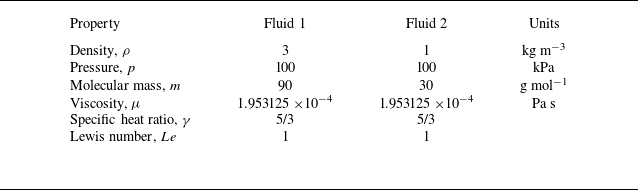


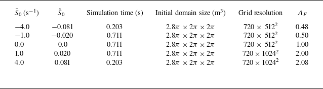


 Open access