


1. Introduction
Long surface gravity waves generate measurable anomalies in the Earth’s magnetic field through the motion of conductive seawater across the geomagnetic field. These signals, detected by seafloor magnetometers and occasionally by low-Earth-orbit satellites, are attracting interest as a complementary tool for tsunami and storm-surge monitoring, see Toh et al. (Reference Toh, Satake, Hamano, Fujii and Goto2011), Wang & Liu (Reference Wang and Liu2013), Minami, Toh & Tyler (Reference Minami, Toh and Tyler2015), Renzi & Mazza (Reference Renzi and Mazza2023) and references therein. Magnetic detection offers the possibility of inferring wave properties without relying solely on direct surface measurements.
Existing theoretical descriptions have focused almost exclusively on constant-depth domains. Tyler (Reference Tyler2005) and Minami et al. (Reference Minami, Toh and Tyler2015) derived closed-form expressions for the magnetic field induced by progressive surface waves, showing proportionality between magnetic and free-surface amplitudes. This scaling holds for uniform depth $h$
, but real waves propagate over variable bathymetry, where the wavenumber
$h$
, but real waves propagate over variable bathymetry, where the wavenumber $k$
varies, and shoaling, refraction and partial reflection occur. Fully numerical hydro-electromagnetic models, such as those of Minami & Toh (Reference Minami and Toh2013) and Minami et al. (Reference Minami, Toh, Ichihara and Kawashima2017), can reproduce these effects, but are computationally intensive, and typically impose artificial boundary conditions that force the magnetic field to vanish at the top and bottom of the computational box. Such constraints are inconsistent with the natural exponential decay of the field and can introduce spurious attenuation unless the vertical extent of the domain greatly exceeds the electromagnetic skin depth.
$k$
varies, and shoaling, refraction and partial reflection occur. Fully numerical hydro-electromagnetic models, such as those of Minami & Toh (Reference Minami and Toh2013) and Minami et al. (Reference Minami, Toh, Ichihara and Kawashima2017), can reproduce these effects, but are computationally intensive, and typically impose artificial boundary conditions that force the magnetic field to vanish at the top and bottom of the computational box. Such constraints are inconsistent with the natural exponential decay of the field and can introduce spurious attenuation unless the vertical extent of the domain greatly exceeds the electromagnetic skin depth.
Here, we bridge this gap by deriving and testing a depth-averaged model for the magnetic field of long waves over slowly varying depth, supported by a new full numerical solution that eliminates box truncation by embedding the exact vertical decay structure analytically at the boundaries. This formulation combines asymptotic accuracy with numerical completeness: it reproduces constant-depth theory in the appropriate limit, captures bathymetric effects without artificial constraints, and isolates the fundamental coupling between hydrodynamic energy flux and electromagnetic induction.
Our results show that the induced magnetic field follows the propagation of wave energy rather than the local free-surface motion, revealing a flux-driven regime of long-wave magnetism that extends classical constant-depth theory to variable bathymetry.
The formulation places tsunami-generated magnetism within a broader class of coupled wave-field problems, where asymptotic analysis and direct simulation jointly expose the leading-order physics hidden from traditional finite-element approaches.
2. Governing equations
We consider a conductive ocean bounded above by air and below by an uneven seabed, as shown in figure 1. In three-dimensional space, let $z$
be a vertical axis pointing upwards, orthogonal to the horizontal
$z$
be a vertical axis pointing upwards, orthogonal to the horizontal $(x,y)$
plane, with
$(x,y)$
plane, with $z=0$
denoting the undisturbed ocean surface. The seabed is located at
$z=0$
denoting the undisturbed ocean surface. The seabed is located at $z=-h(x,y)$
and
$z=-h(x,y)$
and $\zeta (x,y,t)$
represents the free-surface elevation, where
$\zeta (x,y,t)$
represents the free-surface elevation, where $t$
denotes time. We assume that the liquid is inviscid and incompressible and that the flow is irrotational (Mei, Stiassnie & Yue Reference Mei, Stiassnie and Yue2005).
$t$
denotes time. We assume that the liquid is inviscid and incompressible and that the flow is irrotational (Mei, Stiassnie & Yue Reference Mei, Stiassnie and Yue2005).
Schematic of the system’s geometry.

Consider long waves, such as tsunamis, storm surges and tides, for which the free-surface amplitude $A$
is much smaller than both the water depth
$A$
is much smaller than both the water depth $h$
and the wavelength
$h$
and the wavelength $\lambda$
, and the shallow-water condition
$\lambda$
, and the shallow-water condition $\delta =kh \ll 1$
is satisfied, with
$\delta =kh \ll 1$
is satisfied, with $k=2\pi /\lambda$
the wavenumber. The shallow-water approximation corresponds to the leading-order term of the full dispersion relation
$k=2\pi /\lambda$
the wavenumber. The shallow-water approximation corresponds to the leading-order term of the full dispersion relation $\omega ^2 = gk\tanh (kh)$
, see Mei et al. (Reference Mei, Stiassnie and Yue2005). For the long-wave regime considered here (
$\omega ^2 = gk\tanh (kh)$
, see Mei et al. (Reference Mei, Stiassnie and Yue2005). For the long-wave regime considered here ( $kh \lesssim 0.3$
), the dispersive correction
$kh \lesssim 0.3$
), the dispersive correction $\tanh (kh)/(kh) - 1 \approx (kh)^2/3$
remains below
$\tanh (kh)/(kh) - 1 \approx (kh)^2/3$
remains below $3\,\%$
and does not affect the leading-order dynamics.
$3\,\%$
and does not affect the leading-order dynamics.
The effect of the magnetic anomaly associated with such surface gravity waves on the oceanic flow field is negligible (Minami et al. Reference Minami, Toh and Tyler2015; Galtier Reference Galtier2016; Renzi & Mazza Reference Renzi and Mazza2023). Hence, the surface gravity and electromagnetic problems are decoupled. Within the framework of linearised potential flow theory, the free-surface elevation satisfies the well-known long-wave equation
 \begin{align} g \boldsymbol{\nabla } \boldsymbol{\cdot }\left (h \boldsymbol{\nabla }\zeta \right )=\frac {\partial ^2\zeta }{\partial ^2 t}, \end{align}
where $g$
is the acceleration due to gravity. The scattered waves generated by the interaction of incident waves with the seabed must be outgoing in the far field as
$g$
is the acceleration due to gravity. The scattered waves generated by the interaction of incident waves with the seabed must be outgoing in the far field as $|\boldsymbol {x}|=|(x,y)|\rightarrow \infty$
(Mei et al. Reference Mei, Stiassnie and Yue2005). We now turn to the magnetic field.
$|\boldsymbol {x}|=|(x,y)|\rightarrow \infty$
(Mei et al. Reference Mei, Stiassnie and Yue2005). We now turn to the magnetic field.
Consider a conductive medium moving with velocity $\boldsymbol {u}$
and characterised by a magnetic diffusivity
$\boldsymbol {u}$
and characterised by a magnetic diffusivity $\eta =(\mu _0\sigma )^{-1}$
, where
$\eta =(\mu _0\sigma )^{-1}$
, where $\mu _0$
is the permeability of free space and
$\mu _0$
is the permeability of free space and $\sigma$
is the electrical conductivity (Minami et al. Reference Minami, Toh and Tyler2015). Within the framework of kinematic dynamo theory, the magnetic anomaly
$\sigma$
is the electrical conductivity (Minami et al. Reference Minami, Toh and Tyler2015). Within the framework of kinematic dynamo theory, the magnetic anomaly $\boldsymbol {b}(\boldsymbol {x},z,t)$
must satisfy the advection–diffusion equation
$\boldsymbol {b}(\boldsymbol {x},z,t)$
must satisfy the advection–diffusion equation
 \begin{align} \frac {\partial \boldsymbol {b}}{\partial t}=\boldsymbol {F}\boldsymbol{\cdot }\boldsymbol{\nabla }\boldsymbol {u}-\boldsymbol {F}\boldsymbol{\nabla } \boldsymbol{\cdot }\boldsymbol {u}+\eta {\nabla} ^2\boldsymbol {b}, \end{align}
where
F
is the steady Earth’s field, see Davidson (Reference Davidson2016). In the liquid region $\varOmega _L= \{\boldsymbol {x}\in \mathbb{R}^2, -h\lt z\lt 0 \}$
, the magnetic anomaly satisfies (2.2) with
$\varOmega _L= \{\boldsymbol {x}\in \mathbb{R}^2, -h\lt z\lt 0 \}$
, the magnetic anomaly satisfies (2.2) with $\boldsymbol {u}$
being the velocity field induced by the long wave (2.1). A similar equation must be satisfied in the air region
$\boldsymbol {u}$
being the velocity field induced by the long wave (2.1). A similar equation must be satisfied in the air region $\varOmega _A= \{\boldsymbol {x}\in \mathbb{R}^2, z\gt 0 \}$
and the seabed region
$\varOmega _A= \{\boldsymbol {x}\in \mathbb{R}^2, z\gt 0 \}$
and the seabed region $\varOmega _S = \{\boldsymbol {x}\in \mathbb{R}^2, z\lt -h \}$
, where
$\varOmega _S = \{\boldsymbol {x}\in \mathbb{R}^2, z\lt -h \}$
, where $\boldsymbol {u}=\boldsymbol {0}$
. Since the electrical conductivity in both air and soil is much lower than that of seawater (Wang & Liu Reference Wang and Liu2013), we consider the limit
$\boldsymbol {u}=\boldsymbol {0}$
. Since the electrical conductivity in both air and soil is much lower than that of seawater (Wang & Liu Reference Wang and Liu2013), we consider the limit $\eta \rightarrow \infty$
for insulating media, such that (2.2) becomes
$\eta \rightarrow \infty$
for insulating media, such that (2.2) becomes
 \begin{align} {\nabla} ^2\boldsymbol {b}=0 \end{align}
for $({\boldsymbol {x}},z)\in \varOmega _A\cup \varOmega _s$
. The small electrical conductivity of the seabed would introduce errors of only a few percent (Minami et al. Reference Minami, Toh and Tyler2015), which can be reasonably neglected (Wang & Liu Reference Wang and Liu2013; Tatehata, Ichihara & Hamano Reference Tatehata, Ichihara and Hamano2015; Renzi & Mazza Reference Renzi and Mazza2023). Finally, we require the magnetic field to remain bounded as
$({\boldsymbol {x}},z)\in \varOmega _A\cup \varOmega _s$
. The small electrical conductivity of the seabed would introduce errors of only a few percent (Minami et al. Reference Minami, Toh and Tyler2015), which can be reasonably neglected (Wang & Liu Reference Wang and Liu2013; Tatehata, Ichihara & Hamano Reference Tatehata, Ichihara and Hamano2015; Renzi & Mazza Reference Renzi and Mazza2023). Finally, we require the magnetic field to remain bounded as $|z|\rightarrow \infty$
and to be continuous at the air–ocean (
$|z|\rightarrow \infty$
and to be continuous at the air–ocean ( $z=0$
) and ocean–seabed (
$z=0$
) and ocean–seabed ( $z=-h$
) interfaces (Moreau Reference Moreau1990; Tyler Reference Tyler2005; Wang & Liu Reference Wang and Liu2013).
$z=-h$
) interfaces (Moreau Reference Moreau1990; Tyler Reference Tyler2005; Wang & Liu Reference Wang and Liu2013).
In the following, we first revisit the solution for constant depth, which will be instrumental in obtaining a novel depth-averaged equation for the magnetic field over a variable seabed.
3. Solution for constant depth
The analysis assumes an inviscid fluid and an electrically insulating seabed, which is appropriate for long-wave conditions where viscous losses and sub-bottom induction are small compared with the free-surface and bulk conductive responses (Wang & Liu Reference Wang and Liu2013). Finite bottom conductivity or hydrodynamic friction would mainly introduce small amplitude damping without altering the flux-governed coupling mechanism described later.
3.1. Wave field
Consider a narrow-banded approach, with harmonic motion of frequency $\omega$
, such that
$\omega$
, such that
 \begin{align} \zeta (\boldsymbol {x},t)=\mathrm{Re}\{\varTheta (\boldsymbol {x})\,\exp (-\mathrm{i}\omega t)\}, \end{align}
where the real part will be omitted from now on for the sake of brevity. Substituting (3.1) into the governing long-wave equation (2.1) and applying separation of variables yields the well-known solution
 \begin{align} \varTheta (\boldsymbol {x})=A_0\exp (\mathrm{i} \boldsymbol {k}\boldsymbol{\cdot }\boldsymbol {x}), \end{align}
where $A_0$
is the constant wave amplitude and
$A_0$
is the constant wave amplitude and $\boldsymbol {k}=(k_x,k_y)$
is the wavenumber satisfying the dispersion relation
$\boldsymbol {k}=(k_x,k_y)$
is the wavenumber satisfying the dispersion relation $\omega =k\sqrt {gh}$
, with
$\omega =k\sqrt {gh}$
, with $k=|\boldsymbol {k}|$
, see Mei et al. (Reference Mei, Stiassnie and Yue2005). The velocity field is given by
$k=|\boldsymbol {k}|$
, see Mei et al. (Reference Mei, Stiassnie and Yue2005). The velocity field is given by $\boldsymbol {u}(\boldsymbol {x},z,t)=\boldsymbol {v}(\boldsymbol {x},z)\exp (-\mathrm{i}\omega t)$
, where the spatial component
$\boldsymbol {u}(\boldsymbol {x},z,t)=\boldsymbol {v}(\boldsymbol {x},z)\exp (-\mathrm{i}\omega t)$
, where the spatial component
 \begin{align} \boldsymbol {v}=-\frac {\mathrm{i} g}{\omega }\boldsymbol{\nabla }\varTheta = \frac {g}{\omega }\boldsymbol {k}\,\varTheta . \end{align}
3.2. Magnetic field
We focus on the vertical component of the magnetic field, as it has promising potential for early-warning applications (Wang & Liu Reference Wang and Liu2013; Renzi & Mazza Reference Renzi and Mazza2023). Similar calculations can be performed for the horizontal components, but we do not present them here. However, they can be derived by following the same steps. The magnetic field is
 \begin{align} \boldsymbol {b}(\boldsymbol {x},z,t)=\boldsymbol{\beta }(\boldsymbol {x},z)\exp (-\mathrm{i} \omega t), \end{align}
with $\boldsymbol{\beta} =(\beta _x,\beta _y,\beta _z)$
. Substituting (3.4) into the governing equation (2.2) and taking the vertical component yields
$\boldsymbol{\beta} =(\beta _x,\beta _y,\beta _z)$
. Substituting (3.4) into the governing equation (2.2) and taking the vertical component yields
 \begin{align} {\nabla} ^2\beta _z+\frac {\mathrm{i}\omega }{\eta }\beta _z=-\frac {\mathrm{i} g F_z}{\omega \eta }{\nabla} ^2\varTheta , \quad (\boldsymbol {x},z)\in \varOmega _L, \end{align}
where subscripts denote the respective scalar components. Similarly, (2.3) becomes
 \begin{align} {\nabla} ^2\beta _z=0, \quad (\boldsymbol {x},z)\in \varOmega _A\cup \varOmega _S. \end{align}
Separation of variables and variation of parameters, together with continuity of $\beta _z$
and
$\beta _z$
and $\partial \beta _z/\partial z$
at the common boundaries
$\partial \beta _z/\partial z$
at the common boundaries $z=0$
and
$z=0$
and $z=-h$
(Tyler Reference Tyler2005; Wang & Liu Reference Wang and Liu2013; Renzi & Mazza Reference Renzi and Mazza2023) yield the full solution
$z=-h$
(Tyler Reference Tyler2005; Wang & Liu Reference Wang and Liu2013; Renzi & Mazza Reference Renzi and Mazza2023) yield the full solution
 \begin{align} \beta _z(\boldsymbol {x},z)=f(z)\varTheta (\boldsymbol {x}), \end{align}
where
 \begin{align} f(z)=-\frac {\mathrm{i} g F_z k^2}{\alpha ^2\omega \eta } \frac {\alpha \sinh (\alpha h/2)}{k\cosh (\alpha h/2)+\alpha \sinh (\alpha h/2)}\exp (-kz) ,\quad z \geqslant 0, \\[-28pt] \nonumber \end{align}
 \begin{align} f(z)=-\frac {\mathrm{i} g F_z k^2}{\alpha ^2\omega \eta }\frac {k\cosh (\alpha h/2)-k\cosh [(h+2z)\alpha /2]+\alpha \sinh (\alpha h/2)}{k\cosh (\alpha h/2)+\alpha \sinh (\alpha h/2)}, \quad -h\leqslant z\leqslant 0, \\[-28pt] \nonumber \end{align}
 \begin{align} f(z)=-\frac {\mathrm{i} g F_z k^2}{\alpha ^2\omega \eta }\frac {\alpha \sinh (\alpha h/2)}{k\cosh (\alpha h/2)+\alpha \sinh (\alpha h/2)}\exp \left [k(z+h)\right ], \quad z\leqslant -h. \\[-2pt] \nonumber \end{align}
In the latter, $\alpha = \sqrt {k^2 - \mathrm{i}\omega /\eta }$
is the complex magnetic wavenumber (Minami et al. Reference Minami, Toh and Tyler2015), with the principal value of the square root taken using a branch cut along the negative real axis. Note that
$\alpha = \sqrt {k^2 - \mathrm{i}\omega /\eta }$
is the complex magnetic wavenumber (Minami et al. Reference Minami, Toh and Tyler2015), with the principal value of the square root taken using a branch cut along the negative real axis. Note that $f(z)$
is
$f(z)$
is $\mathrm{C}^1(\mathbb{R})$
to satisfy the continuity conditions at the air–liquid and liquid–soil interfaces, and
$\mathrm{C}^1(\mathbb{R})$
to satisfy the continuity conditions at the air–liquid and liquid–soil interfaces, and $f\rightarrow 0$
exponentially as
$f\rightarrow 0$
exponentially as $|z|\rightarrow \infty$
. In the limit
$|z|\rightarrow \infty$
. In the limit $kh\rightarrow 0$
, (3.7) and (3.9) together yield
$kh\rightarrow 0$
, (3.7) and (3.9) together yield
 \begin{align} \frac {\beta _z}{F_z}= \frac {\sqrt {gh}}{h\sqrt {gh}+2\mathrm{i}\eta }\varTheta , \end{align}
which is identical to the constant-depth expression of Tyler (Reference Tyler2005) (see also Renzi & Mazza Reference Renzi and Mazza2023). Although derived for uniform depth, this amplitude law is often applied locally by replacing $h\rightarrow h(x)$
(e.g. Tyler Reference Tyler2005; Minami et al. Reference Minami, Toh and Tyler2015); we assess the validity of that ad hoc extension in § 7.
$h\rightarrow h(x)$
(e.g. Tyler Reference Tyler2005; Minami et al. Reference Minami, Toh and Tyler2015); we assess the validity of that ad hoc extension in § 7.
Substitution of (3.7) into (3.5) and (3.6) reveals that $f$
satisfies
$f$
satisfies
 \begin{align} \frac {\partial ^2 \kern-2pt f}{\partial z^2}-\alpha^2 \kern-2pt f=\frac {\mathrm{i} F_z g k^2}{\omega \eta }, \quad (\boldsymbol {x},z)\in \varOmega _L, \end{align}
and
 \begin{align} \frac {\partial ^2 \kern-2pt f}{\partial z^2}-k^2 \kern-2pt f=0,\quad (\boldsymbol {x},z)\in \varOmega _A\cup \varOmega _S, \end{align}
which can be readily verified using (3.8)–(3.10). We now derive a depth-averaged equation for the vertical magnetic field over variable depth.
4. Depth-averaged equation for the magnetic field
We consider slowly varying bathymetry such that $\epsilon = |\boldsymbol{\nabla }h|/(k h) \ll 1$
. While the long-wave parameter
$\epsilon = |\boldsymbol{\nabla }h|/(k h) \ll 1$
. While the long-wave parameter $\delta = k h$
controls the vertical structure,
$\delta = k h$
controls the vertical structure, $\epsilon$
governs the horizontal modulation. In the mild-slope limit, we assume that the vertical structure of the magnetic field remains that of the constant-depth solution
$\epsilon$
governs the horizontal modulation. In the mild-slope limit, we assume that the vertical structure of the magnetic field remains that of the constant-depth solution $f$
given by (3.8)–(3.10), with only a weak, parametric dependence on the local depth
$f$
given by (3.8)–(3.10), with only a weak, parametric dependence on the local depth $h(\boldsymbol{x})$
. Accordingly, we seek a separable solution of the form
$h(\boldsymbol{x})$
. Accordingly, we seek a separable solution of the form
 \begin{align} \beta _z(\boldsymbol{x},z) = f\!\left (z,\,h(\boldsymbol{x})\right )\,X(\boldsymbol{x}), \end{align}
where $X(\boldsymbol{x})$
varies on the slow horizontal scale
$X(\boldsymbol{x})$
varies on the slow horizontal scale $O(1/\epsilon )$
. The governing equations (3.5)–(3.6) are valid for variable depth; however, we now rewrite them as
$O(1/\epsilon )$
. The governing equations (3.5)–(3.6) are valid for variable depth; however, we now rewrite them as
 \begin{align} \frac {\partial ^2\beta _z}{\partial z^2}+{\nabla} ^2_2\,\beta _z+\frac {\mathrm{i}\omega }{\eta }\beta _z=-\frac {\mathrm{i} g F_z}{\omega \eta }{\nabla} ^2_2\varTheta , \quad (\boldsymbol {x},z)\in \varOmega _L, \end{align}
and
 \begin{align} \frac {\partial ^2\beta _z}{\partial z^2}+{\nabla} ^2_2\,\beta _z=0, \quad (\boldsymbol {x},z)\in \varOmega _A\cup \varOmega _S, \end{align}
respectively, where $\boldsymbol{\nabla} _2=(\partial /\partial x,\partial /\partial y)$
is the horizontal gradient. We also request that
$\boldsymbol{\nabla} _2=(\partial /\partial x,\partial /\partial y)$
is the horizontal gradient. We also request that $\beta _z$
be finite as
$\beta _z$
be finite as $|z|\rightarrow \infty$
.
$|z|\rightarrow \infty$
.
Now, regard (4.2)–(4.3) as ordinary differential equations in $z$
and apply Green’s second identity separately in each region, using (3.12)–(3.13) for
$z$
and apply Green’s second identity separately in each region, using (3.12)–(3.13) for $f$
, so that
$f$
, so that
 \begin{align} \int _{-\infty }^{-h}\left (f(-{\nabla} ^2_2\,\beta _z)-\beta _z k^2 f \right )\,{\mathrm{d}} z=\left [f\frac {\partial \beta _z}{\partial z}-\beta _z\frac {\partial f}{\partial z} \right ]_{z=-h} \!, \nonumber \\[-28pt] \end{align}
 \begin{align} & \qquad \int _{-h}^0\left [f\left (-{\nabla} ^2_2\,\beta _z-\frac {\mathrm{i}\omega }{\eta }\beta _z-\frac {\mathrm{i} g F_z}{\omega \eta } {\nabla} ^2_2\varTheta \right ) -\beta _z\left (\alpha ^2f+\frac {\mathrm{i} F_z g k^2}{\omega \eta }\right )\right ]\,{\mathrm{d}} z \nonumber \\& =\left [f\frac {\partial \beta _z}{\partial z}-\beta _z\frac {\partial f}{\partial z} \right ]_{z=-h}^{z=0} \\[-2pt] \nonumber \end{align}
and
 \begin{align} \int _0^\infty \left (f(-{\nabla} ^2_2\,\beta _z)-\beta _zk^2 \kern-2pt f \right )\,{\mathrm{d}} z=-\left [f\frac {\partial \beta _z}{\partial z}-\beta _z\frac {\partial f}{\partial z} \right ]_{z=0}. \end{align}
Using (4.1), the horizontal Laplacian becomes
 \begin{align} {\nabla} ^2_2\,\beta _z=f{\nabla} ^2_2 X+2\frac {\partial f}{\partial h}\boldsymbol{\nabla} _2 X\boldsymbol{\cdot }\boldsymbol{\nabla} _2 h+X\,\frac {\partial ^2 \kern-2pt f}{\partial h^2}\left (\boldsymbol{\nabla} _2 h \right )^2+X\frac {\partial f}{\partial h}{\nabla} _2^2h. \end{align}
Consider the depth-averaged integral (4.5) for the liquid layer. Substituting (3.7), (4.7) in (4.5) and using (4.4), (4.6) as boundary conditions at $z=-h$
and
$z=-h$
and $z=0$
, respectively, yields
$z=0$
, respectively, yields
 \begin{eqnarray} &&{\nabla} ^2_2 X\int _{-h}^{0}f^2\,{\mathrm{d}} z+2\boldsymbol{\nabla} _2X\boldsymbol {\cdot }\boldsymbol{\nabla} _2h\int _{-h}^{0}f\frac {\partial f}{\partial h}\,{\mathrm{d}} z+X\int _{-h}^0f\frac {\partial ^2 \kern-2pt f}{\partial h^2}\,{\mathrm{d}} z\, (\boldsymbol{\nabla} _2h)^2\nonumber \\&&+X\int _{-h}^0f\frac {\partial f}{\partial h}\,{\mathrm{d}} z\,{\nabla} ^2_2h+\frac {\mathrm{i}\omega }{\eta }X\int _{-h}^0 f^2\,{\mathrm{d}} z+\frac {\mathrm{i} F_zg}{\omega \eta }{\nabla} ^2_2\varTheta \int _{-h}^0f\,{\mathrm{d}} z+X\alpha ^2\int _{-h}^0f^2\,{\mathrm{d}} z\nonumber \\&&+X\frac {\mathrm{i} F_zgk^2}{\omega \eta }\int _{-h}^0f\,{\mathrm{d}} z=-{\nabla} ^2_2X\int _0^{+\infty }f^2\,{\mathrm{d}} z-2\boldsymbol{\nabla} _2 X \boldsymbol{\cdot }\boldsymbol{\nabla} _2h\int _0^{+\infty }f\frac {\partial f}{\partial h}\,{\mathrm{d}} z\nonumber \\&&-X\int _0^{+\infty }f\frac {\partial ^2f}{\partial h^2}\,{\mathrm{d}} z\,(\boldsymbol{\nabla} _2h)^2-X\int _0^{+\infty }f\frac {\partial f}{\partial h}\,{\mathrm{d}} z\,{\nabla} ^2_2 h-Xk^2\int _0^{+\infty }f^2\,{\mathrm{d}} z\nonumber \\&&-{\nabla} ^2_2X\int _{-\infty }^{-h}f^2\,{\mathrm{d}} z-2\boldsymbol{\nabla} _2X\boldsymbol{\cdot }\boldsymbol{\nabla} _2h\int _{-\infty }^{-h}f\frac {\partial f}{\partial h}\,{\mathrm{d}} z-X\int _{-\infty }^{-h}f\frac {\partial ^2 \kern-2pt f}{\partial h^2}\,{\mathrm{d}} z\,(\boldsymbol{\nabla} _2h)^2\nonumber \\&&-X\int _{-\infty }^{-h}f\frac {\partial f}{\partial h}\,{\mathrm{d}} z\,{\nabla} _2^2h-Xk^2\int _{-\infty }^{-h}f^2\,{\mathrm{d}} z. \end{eqnarray}
Collecting terms proportional to ${\nabla} ^2_2X$
,
${\nabla} ^2_2X$
, $\boldsymbol{\nabla} _2X \boldsymbol{\cdot }\boldsymbol{\nabla} _2h$
and
$\boldsymbol{\nabla} _2X \boldsymbol{\cdot }\boldsymbol{\nabla} _2h$
and $X$
, and recalling that
$X$
, and recalling that $f$
in (3.8)–(3.10) is integrable over the full domain
$f$
in (3.8)–(3.10) is integrable over the full domain $z\in \mathbb{R}$
, (4.8) simplifies into
$z\in \mathbb{R}$
, (4.8) simplifies into
 \begin{eqnarray} {\nabla} ^2_2 X\int _{-\infty }^{+\infty }f^2\,{\mathrm{d}} z+2\boldsymbol{\nabla} _2X\boldsymbol{\cdot }\boldsymbol{\nabla} _2h\int _{-\infty }^{+\infty }f\frac {\partial f}{\partial h}\,{\mathrm{d}} z+k^2X\int _{-\infty }^{+\infty }f^2\,{\mathrm{d}} z\nonumber \\ +\frac {\mathrm{i} g F_z}{\omega \eta }\left (k^2X+{\nabla} _2^2\varTheta \right )\int _{-h}^{0}f\,{\mathrm{d}} z=O \big(({\nabla} _2 h)^2 \big)+O \big({\nabla} _2^2 h \big), \end{eqnarray}
where the integrals can be calculated analytically, as detailed in Appendix A.
Equation (4.9) represents the electromagnetic analogue of the classical mild-slope equation in the long-wave limit. It governs the slowly varying horizontal amplitude $X(\boldsymbol {x})$
of the vertical magnetic field
$X(\boldsymbol {x})$
of the vertical magnetic field $\beta _z$
(3.7) within the liquid layer
$\beta _z$
(3.7) within the liquid layer $\varOmega _L$
, induced by the long-wave potential
$\varOmega _L$
, induced by the long-wave potential $\varTheta (\boldsymbol {x})$
over a gently varying seabed.
$\varTheta (\boldsymbol {x})$
over a gently varying seabed.
Under the long-wave and mild-slope assumptions, $\delta =kh\ll 1$
and
$\delta =kh\ll 1$
and $\epsilon = |\boldsymbol{\nabla} _2 h|/(k h) \ll 1$
, and hence,
$\epsilon = |\boldsymbol{\nabla} _2 h|/(k h) \ll 1$
, and hence, $|\boldsymbol{\nabla} _2 h|\ll \delta \ll 1$
. The terms proportional to
$|\boldsymbol{\nabla} _2 h|\ll \delta \ll 1$
. The terms proportional to ${\nabla} _2^2$
and to
${\nabla} _2^2$
and to $k^2$
on the left-hand side of (4.9) are
$k^2$
on the left-hand side of (4.9) are $O(\delta ^2)$
, and provide the leading contribution. The mixed topographic term
$O(\delta ^2)$
, and provide the leading contribution. The mixed topographic term $\boldsymbol{\nabla} _2 X\!\boldsymbol{\cdot }\!\boldsymbol{\nabla} _2 h$
is
$\boldsymbol{\nabla} _2 X\!\boldsymbol{\cdot }\!\boldsymbol{\nabla} _2 h$
is $O(\epsilon \,\delta ^2)$
and introduces the slow horizontal modulation. By contrast, the slope-squared and curvature remainders,
$O(\epsilon \,\delta ^2)$
and introduces the slow horizontal modulation. By contrast, the slope-squared and curvature remainders, $(\boldsymbol{\nabla} _2 h)^2$
and
$(\boldsymbol{\nabla} _2 h)^2$
and ${\nabla} _2^2 h$
, scale as
${\nabla} _2^2 h$
, scale as $O(\epsilon ^2\delta ^2)$
and are therefore neglected at the present order. Accordingly, we retain terms up to
$O(\epsilon ^2\delta ^2)$
and are therefore neglected at the present order. Accordingly, we retain terms up to $O(\epsilon \,\delta ^2)$
in what follows.
$O(\epsilon \,\delta ^2)$
in what follows.
4.1. Mild-slope form of the depth-integrated equation
For a generic depth $h(x,y)$
, we define the depth-integrated coefficients associated with the electromagnetic vertical mode
$h(x,y)$
, we define the depth-integrated coefficients associated with the electromagnetic vertical mode $f(z,h)$
as
$f(z,h)$
as
 \begin{align} A(h)=\int _{-\infty }^{\infty } f^{2}\,{\rm d}z, \qquad B(h)=\int _{-\infty }^{\infty } f\,\frac {\partial f}{\partial h}\,{\rm d}z, \qquad C(h)=\int _{-h}^{0} f\,{\rm d}z, \end{align}
which satisfy the exact differential identity
 \begin{align} \frac {{\rm d}A}{{\rm d}h}=2B. \end{align}
Here, $A$
measures the vertical magnetic energy density,
$A$
measures the vertical magnetic energy density, $B$
controls the first-order coupling with bottom slope and
$B$
controls the first-order coupling with bottom slope and $C$
controls the electromagnetic coupling through
$C$
controls the electromagnetic coupling through ${\nabla} ^2_2\varTheta$
.
${\nabla} ^2_2\varTheta$
.
Equation (4.9) can then be expressed in the mild-slope form
 \begin{align} \boldsymbol{\nabla} _2\!\boldsymbol{\cdot }\!\big (A(h)\,\boldsymbol{\nabla} _2 X\big ) + A(h)\,k^{2}(1+r)\,X = -A(h)r{\nabla} _2^{2}\varTheta , \qquad r=\frac {\textit{igF}_z}{\omega \eta }\frac {C}{A}, \end{align}
which is formally analogous to Berkhoff’s mild-slope equation for surface gravity waves (Mei et al. Reference Mei, Stiassnie and Yue2005). Both equations describe the lateral propagation of a depth-modulated mode governed by a weighting coefficient, but they differ in physical interpretation. In Berkhoff’s theory, the unknown is the free-surface elevation and the weight $a=\textit{cC}_g$
(with
$a=\textit{cC}_g$
(with $c$
being the phase speed and
$c$
being the phase speed and $C_g$
the group speed) arises from wave-action conservation. Here, by contrast, the unknown
$C_g$
the group speed) arises from wave-action conservation. Here, by contrast, the unknown $X$
represents the electromagnetic field induced by the moving surface and
$X$
represents the electromagnetic field induced by the moving surface and $A(h)$
originates from the vertical mode
$A(h)$
originates from the vertical mode $f(z,h)$
, measuring the magnetic energy stored in the system. Finally, the complex coupling
$f(z,h)$
, measuring the magnetic energy stored in the system. Finally, the complex coupling $r$
introduces magnetic diffusion, breaking the self-adjoint character of Berkhoff’s operator.
$r$
introduces magnetic diffusion, breaking the self-adjoint character of Berkhoff’s operator.
5. Numerical solution
Existing numerical models of tsunami-generated electromagnetic fields, such as the finite-element formulations of Minami & Toh (Reference Minami and Toh2013) and Minami et al. (Reference Minami, Toh, Ichihara and Kawashima2017), solve the induction equations in a finite domain under Dirichlet-type boundary conditions that force the magnetic field to vanish at the top and bottom boundaries of the computational domain. Although acceptable for sufficiently large domains, this treatment does not reproduce the true exponential decay of the field and may introduce artificial attenuation unless the domain height greatly exceeds the electromagnetic skin depth. The analytical framework introduced in § 3 embeds the correct vertical structure of the field, eliminating the need for artificial boundaries and providing the basis for a more computationally efficient and physically consistent solution.
5.1. Formulation
We construct a full numerical model based on a step approximation of the wave and electromagnetic fields. This procedure coincides algebraically with the transition-matrix formalism of Devillard, Dunlop & Souillard (Reference Devillard, Dunlop and Souillard1988) and with the generalised version of Evans & Linton (Reference Evans and Linton1994). Here, the discretisation is applied directly to the bathymetry, making it a projection of the full operator onto a piecewise-constant (Haar) subspace in the physical plane. While the approach itself is not new, to our knowledge, this is the first time it has been applied to the magnetic field in the context of wave-induced electromagnetism.
This formulation is two-dimensional in the $(x,z)$
plane; an extension to fully three-dimensional (3-D) bathymetries can be obtained by applying the same step-wise matching procedure independently in the transverse direction, leading to coupled 3-D transfer relations.
$(x,z)$
plane; an extension to fully three-dimensional (3-D) bathymetries can be obtained by applying the same step-wise matching procedure independently in the transverse direction, leading to coupled 3-D transfer relations.
We seek a time-harmonic solution $\zeta (x,t)=\mathrm{Re}\{\varTheta (x)\,{\rm e}^{-{i}\omega t}\}$
, which gives the scalar ordinary differential equation (ODE)
$\zeta (x,t)=\mathrm{Re}\{\varTheta (x)\,{\rm e}^{-{i}\omega t}\}$
, which gives the scalar ordinary differential equation (ODE)
 \begin{align} \big (h(x)\,\varTheta '\big )' + \frac {\omega ^2}{g}\,\varTheta = 0, \end{align}
where primes denote differentiation and the bathymetry smoothly connects to constant-depth regions as $x\rightarrow \pm \infty$
, where standard radiation conditions are imposed (Mei et al. Reference Mei, Stiassnie and Yue2005).
$x\rightarrow \pm \infty$
, where standard radiation conditions are imposed (Mei et al. Reference Mei, Stiassnie and Yue2005).
5.2. Step approximation and Haar projection
To obtain a tractable full numerical solution without slope assumptions, the bottom profile is replaced by a piecewise-constant function
 \begin{align} h(x) \approx \sum _{j=1}^{N} h_{\kern-1.5pt j}\,\chi _j(x), \qquad \chi _j(x) = \begin{cases} 1, & x_{j-1} \lt x \lt x_{\kern-1.5pt j},\\[3pt] 0, & \text{otherwise,} \end{cases}\quad j=1,\ldots ,N. \end{align}
The functions $\chi _j(x)$
form a Haar-type basis. Projecting (5.1) onto this subspace yields, on each strip
$\chi _j(x)$
form a Haar-type basis. Projecting (5.1) onto this subspace yields, on each strip $j$
,
$j$
,
 \begin{align} \varTheta '' + k_{\kern-1.5pt j}^2\,\varTheta = 0,\qquad k_{\kern-1.5pt j}^2 = \frac {\omega ^2}{\textit{gh}_{\kern-1.5pt j}},\qquad x_{j-1}\lt x\lt x_{\kern-1.5pt j}, \end{align}
whose general solution is
 \begin{align} \varTheta _{\kern-1.5pt j}(x) = T_{\kern-1.5pt j}\,{\mathrm{exp}}\big(\mathrm{i} k_{\kern-1.5pt j} x \big) + R_{\kern-1.5pt j}\,{\mathrm{exp}} \big({-}\mathrm{i} k_{\kern-1.5pt j} x \big), \end{align}
where $T_{\kern-1.5pt j}$
and
$T_{\kern-1.5pt j}$
and $R_{\kern-1.5pt j}$
are unknown complex values. The computational domain is truncated at
$R_{\kern-1.5pt j}$
are unknown complex values. The computational domain is truncated at $x_0 = x_L$
on the left and
$x_0 = x_L$
on the left and $x_{N+1} = x_R$
on the right, representing the constant-depth regions as
$x_{N+1} = x_R$
on the right, representing the constant-depth regions as $x \to \pm \infty$
. Boundary conditions are imposed by prescribing a unit incident amplitude from the left (
$x \to \pm \infty$
. Boundary conditions are imposed by prescribing a unit incident amplitude from the left ( $T_0 = 1$
) and no incoming wave from the right (
$T_0 = 1$
) and no incoming wave from the right ( $R_{N+1} = 0$
).
$R_{N+1} = 0$
).
At each step $x=x_{\kern-1.5pt j}$
, we enforce
$x=x_{\kern-1.5pt j}$
, we enforce
 \begin{align} \varTheta _{\kern-1.5pt j}=\varTheta _{\kern-1.5pt j+1},\qquad h_{\kern-1.5pt j}\,\varTheta '_{\kern-1.5pt j} = h_{\kern-1.5pt j+1}\,\varTheta '_{\kern-1.5pt j+1}, \end{align}
i.e. continuity of surface elevation and mass flux. This yields a system of $2N+2$
equations in as many unknowns,
$2N+2$
equations in as many unknowns,
 \begin{align} & T_{\kern-1.5pt j}\,\exp \big(\mathrm{i} k_{\kern-1.5pt j}x_{\kern-1.5pt j}\big)+R_{\kern-1.5pt j}\,\exp \big({-}\mathrm{i} k_{\kern-1.5pt j} x_{\kern-1.5pt j}\big)-T_{\kern-1.5pt j+1}\,\exp \big(\mathrm{i} k_{\kern-1.5pt j+1}x_{\kern-1.5pt j}\big)-R_{\kern-1.5pt j+1}\,{\mathrm{exp}}\big({-}\mathrm{i} k_{\kern-1.5pt j+1}x_{\kern-1.5pt j}\big)=0, \\[-12pt] \nonumber \end{align}
 \begin{align} &T_{\kern-1.5pt j}\mathrm{i} k_{\kern-1.5pt j}h_{\kern-1.5pt j}\,{\mathrm{exp}} \big(\mathrm{i} k_{\kern-1.5pt j}x_{\kern-1.5pt j}\big)-R_{\kern-1.5pt j}\mathrm{i} k_{\kern-1.5pt j} h_{\kern-1.5pt j}\,{\mathrm{exp}}\big({-}\mathrm{i} k_{\kern-1.5pt j}x_{\kern-1.5pt j}\big)-T_{\kern-1.5pt j+1}\mathrm{i} k_{\kern-1.5pt j+1}h_{\kern-1.5pt j+1}\,{\mathrm{exp}}\big(\mathrm{i} k_{\kern-1.5pt j+1}x_{\kern-1.5pt j}\big)\nonumber \\ & \quad +R_{\kern-1.5pt j+1}\mathrm{i} k_{\kern-1.5pt j+1}h_{\kern-1.5pt j+1}\,{\mathrm{exp}}\big({-}\mathrm{i} k_{\kern-1.5pt j+1}x_{\kern-1.5pt j}\big)=0. \\[9pt] \nonumber \end{align}
Energy conservation requires
 \begin{align} E = |R_0|^2 + \sqrt {\frac {h_{\kern-1pt R}}{h_{\kern-1pt L}}}\,|T_{N+1}|^2 = 1, \end{align}
and deviations of $E$
from unity provide a convergence diagnostic.
$E$
from unity provide a convergence diagnostic.
The magnetic field is obtained by applying, on each constant-depth strip, the exact linear constant-depth transfer relation
 \begin{align} \beta _{z_j}(x) = f_{\kern-1.5pt j}(-h_{\kern-1.5pt j})\,\varTheta _{\kern-1.5pt j}(x), \end{align}
where $f_{\kern-1.5pt j}$
denotes the Haar projection of (3.8)–(3.10) and embeds the electromagnetic coupling for depth
$f_{\kern-1.5pt j}$
denotes the Haar projection of (3.8)–(3.10) and embeds the electromagnetic coupling for depth $h_{\kern-1.5pt j}$
. This represents a quasi-local induction approximation, as the vertical electromagnetic structure is solved exactly within each strip, while lateral coupling between adjacent strips is neglected. The approach is asymptotically valid when
$h_{\kern-1.5pt j}$
. This represents a quasi-local induction approximation, as the vertical electromagnetic structure is solved exactly within each strip, while lateral coupling between adjacent strips is neglected. The approach is asymptotically valid when
 \begin{align} \Delta x = x_{\kern-1.5pt j+1}-x_{\kern-1.5pt j} \ll \min \!\big (\lambda ,\ \delta _{\textit{EM}}\big ), \qquad \delta _{\textit{EM}} = \sqrt {\frac {2\eta }{\omega }}, \end{align}
so that both the hydrodynamic wavelength $\lambda$
and the electromagnetic skin depth
$\lambda$
and the electromagnetic skin depth $\delta _{\textit{EM}}$
exceed the strip width. No depth-integrated or mild-slope separation is invoked in this formulation, which therefore constitutes a fully numerical solution.
$\delta _{\textit{EM}}$
exceed the strip width. No depth-integrated or mild-slope separation is invoked in this formulation, which therefore constitutes a fully numerical solution.
6. Model implementation and validation
6.1. Depth-averaged model
6.1.1. General approach
Equation (4.9) is solved numerically for prescribed bathymetric profiles $h(\boldsymbol {x})$
. In the present work, we focus on parallel depth contours
$h(\boldsymbol {x})$
. In the present work, we focus on parallel depth contours $h=h(x)$
. The depth-averaged (4.9) becomes
$h=h(x)$
. The depth-averaged (4.9) becomes
 \begin{align} L(X)=X''+h'p(h(x))X'+q(h(x))X+r(h(x))\varTheta ''=0, \end{align}
where primes denote differentiation with respect to $x$
and
$x$
and
 \begin{align} p(h(x))=\frac {2B}{A}; \; q(h(x))=k^2(1+r(h(x)). \end{align}
The latter expressions depend on the electromagnetic structure through $f(z)$
and have analytical expressions upon substitution of (A1)–(A3). Boundary conditions depend on the particular geometry being investigated and are detailed in the validation § 6.3.
$f(z)$
and have analytical expressions upon substitution of (A1)–(A3). Boundary conditions depend on the particular geometry being investigated and are detailed in the validation § 6.3.
6.1.2. Treatment of slope discontinuities
Canonical piecewise-linear bottom profiles, consisting of flat regions connected by planar slopes, have been widely employed in the study of coastal and tsunami wave propagation (e.g. Dingemans Reference Dingemans1997; Sammarco et al. Reference Sammarco, Cecioni, Bellotti and Abdolali2013; Abdolali, Kirby & Bellotti Reference Abdolali, Kirby and Bellotti2015). In such configurations, the bottom derivative $h'$
is discontinuous at a junction
$h'$
is discontinuous at a junction $x_c$
and, therefore, must be handled carefully within the depth-integrated framework. This is because the step discontinuity in
$x_c$
and, therefore, must be handled carefully within the depth-integrated framework. This is because the step discontinuity in $h'$
at
$h'$
at $x_c$
introduces distributional terms
$x_c$
introduces distributional terms $h''\propto \delta (x-x_c)$
, which make the contribution from the
$h''\propto \delta (x-x_c)$
, which make the contribution from the $O({\nabla} ^2_2 h)$
terms in (4.9) non-negligible.
$O({\nabla} ^2_2 h)$
terms in (4.9) non-negligible.
Consider the governing equation (4.8) and retain the terms $O({\nabla} _2^2 h)$
on the right-hand side,
$O({\nabla} _2^2 h)$
on the right-hand side,
 \begin{align} \text{right-hand side} = - \textit{XB}{\nabla} ^2_2h. \end{align}
Writing again the equation in conservative form, considering the two-dimensional limit and integrating across an infinitesimal control volume surrounding a junction point $x_c$
yields the formal jump condition
$x_c$
yields the formal jump condition
 \begin{align} \big [A(h)X'\big ] = -\,B(h)[h']X. \end{align}
In the latter expression, $[f]$
denotes the jump of
$[f]$
denotes the jump of $f(x)$
across
$f(x)$
across $x_c$
. Using (4.10), the jump condition (6.4) becomes
$x_c$
. Using (4.10), the jump condition (6.4) becomes
 \begin{align} X'\big(x_c^+ \big)=X'\big(x_c^- \big)-\frac {p(x_c)}{2}\Delta h'(x_c)X(x_c), \end{align}
where $\Delta h'(x_c)$
is the jump in steepness at
$\Delta h'(x_c)$
is the jump in steepness at $x_c$
. This Rankine–Hugoniot-type condition ensures conservation of the depth-integrated electromagnetic flux across the slope breaks while maintaining continuity of the field
$x_c$
. This Rankine–Hugoniot-type condition ensures conservation of the depth-integrated electromagnetic flux across the slope breaks while maintaining continuity of the field $X$
. In the numerical implementation, the jump is imposed explicitly at a discontinuity point
$X$
. In the numerical implementation, the jump is imposed explicitly at a discontinuity point $x_c$
through a local update of
$x_c$
through a local update of $X'$
, which reproduces the finite discontinuity predicted by the asymptotic theory and avoids spurious reflections. As
$X'$
, which reproduces the finite discontinuity predicted by the asymptotic theory and avoids spurious reflections. As $\Delta h'\!\to \!0$
, (6.5) recovers the smooth mild-slope limit.
$\Delta h'\!\to \!0$
, (6.5) recovers the smooth mild-slope limit.
6.2. Full numerical model
The numerical implementation assembles the matrix (5.6)–(5.7), solves for the coefficients $(T_{\kern-1.5pt j},R_{\kern-1.5pt j})$
using sparse linear algebra, and reconstructs the free-surface elevation and derived quantities (e.g. magnetic perturbations) along the domain. Increasing the number of steps
$(T_{\kern-1.5pt j},R_{\kern-1.5pt j})$
using sparse linear algebra, and reconstructs the free-surface elevation and derived quantities (e.g. magnetic perturbations) along the domain. Increasing the number of steps $N$
results in converged solutions, with the total energy balance satisfied to excellent precision
$N$
results in converged solutions, with the total energy balance satisfied to excellent precision $O(10^{-14})$
, see Appendix B.
$O(10^{-14})$
, see Appendix B.
6.3. Validation of the depth-averaged model
6.3.1. Analytical validation
First, we consider the case of constant depth, $h=h_0$
, for which
$h=h_0$
, for which $\varTheta =A_0\exp (\mathrm{i} kx)$
. The depth-averaged (6.1) is solved numerically using periodic boundary conditions, i.e.
$\varTheta =A_0\exp (\mathrm{i} kx)$
. The depth-averaged (6.1) is solved numerically using periodic boundary conditions, i.e. $X(0)=X(\lambda )$
, where
$X(0)=X(\lambda )$
, where $\lambda =2\pi /k$
. The numerical solution is obtained with Mathematica(R) using an explicit Runge–Kutta scheme of order 8. The computational time on an Intel(R) Core(TM) i7-10700 machine equipped with a 2.90 GHz CPU and 64 GB RAM is
$\lambda =2\pi /k$
. The numerical solution is obtained with Mathematica(R) using an explicit Runge–Kutta scheme of order 8. The computational time on an Intel(R) Core(TM) i7-10700 machine equipped with a 2.90 GHz CPU and 64 GB RAM is $O(2\ \mathrm{s})$
. Figure 2 shows the behaviour of
$O(2\ \mathrm{s})$
. Figure 2 shows the behaviour of $X(x)$
over a wavelength, compared with the analytical solution for constant depth obtained in § 3. Parameters are
$X(x)$
over a wavelength, compared with the analytical solution for constant depth obtained in § 3. Parameters are $h=4000\,\mathrm{m}$
,
$h=4000\,\mathrm{m}$
, $F_z=-20\,000\,\mathrm{nT}$
,
$F_z=-20\,000\,\mathrm{nT}$
, $\eta =198\,944\,\mathrm{m}^2\,\mathrm{s}^{-1}$
and a period of
$\eta =198\,944\,\mathrm{m}^2\,\mathrm{s}^{-1}$
and a period of $600\,\mathrm{s}$
. The numerical and analytical curves are visually indistinguishable. We quantify the agreement using the relative
$600\,\mathrm{s}$
. The numerical and analytical curves are visually indistinguishable. We quantify the agreement using the relative $\textit{L}_2$
norm,
$\textit{L}_2$
norm,
 \begin{align} \textit{L}_2=\frac {||X_{\textit{num}}-X_{\textit{ana}}||_2}{||X_{\textit{ana}}||_2}, \end{align}
which measures the root-mean-square (r.m.s) difference, and the relative infinity norm,
 \begin{align} L_{\infty} =\frac {\max |X_{\textit{num}}-X_{\textit{ana}}|}{\max |X_{\textit{ana}}|}, \end{align}
which measures the worst pointwise error, where $X_{\textit{num}}$
and
$X_{\textit{num}}$
and $X_{\textit{ana}}$
represent the numerical and analytical solutions, respectively (Miller, Renzi & Discacciati Reference Miller, Renzi and Discacciati2025). We have
$X_{\textit{ana}}$
represent the numerical and analytical solutions, respectively (Miller, Renzi & Discacciati Reference Miller, Renzi and Discacciati2025). We have $\textit{L}_2=4.9\times 10^{-9}$
and
$\textit{L}_2=4.9\times 10^{-9}$
and $\textit{L}_\infty =2.2\times 10^{-8}$
providing robust validation of (4.9) in the case of constant depth.
$\textit{L}_\infty =2.2\times 10^{-8}$
providing robust validation of (4.9) in the case of constant depth.
Plot of $\mathrm{Re}\{X (x)\}$
for constant depth
$\mathrm{Re}\{X (x)\}$
for constant depth $h=4000\,\mathrm{m}$
, obtained with the numerical solution (- -) of the depth-averaged (6.1) and the analytical solution (
$h=4000\,\mathrm{m}$
, obtained with the numerical solution (- -) of the depth-averaged (6.1) and the analytical solution (![]() ), for
), for $t=600\,\mathrm{s}$
and
$t=600\,\mathrm{s}$
and $A_0=1\,\mathrm{m}$
.
$A_0=1\,\mathrm{m}$
.

6.3.2. Numerical validation
We now validate the depth-integrated model against the full numerical model for varying bathymetry. As a commonly used benchmark test (Sammarco et al. Reference Sammarco, Cecioni, Bellotti and Abdolali2013; Abdolali et al. Reference Abdolali, Kirby and Bellotti2015), we examine a configuration consisting of two regions of constant depth connected by a sloping transition. The water depth is $h=h_0$
for
$h=h_0$
for $x\lt 0$
and
$x\lt 0$
and $h=h_1$
for
$h=h_1$
for $x\gt x_1$
, while in the transition region of variable depth, it is given by
$x\gt x_1$
, while in the transition region of variable depth, it is given by $h=h_0-mx$
, ensuring that
$h=h_0-mx$
, ensuring that $h_1=h_0-mx_1$
.
$h_1=h_0-mx_1$
.
The wave field admits an analytical solution, found by solving the wave equation (2.1) separately in each region, and matching pressure and fluxes at the common boundaries at $x=0$
and
$x=0$
and $x=x_1$
. This yields
$x=x_1$
. This yields
 \begin{align} \varTheta =\exp (\mathrm{i}k_0x)+R\exp (-\mathrm{i} k_0x), \quad x\lt 0, \\[-28pt] \nonumber \end{align}
 \begin{align} \varTheta =R_0J_0\left (2\sqrt {s(h_0-mx)}\right )+T_0Y_0\left (2\sqrt {s(h_0-mx)}\right ), \quad 0\lt x\lt x_1, \\[-28pt] \nonumber \end{align}
 \begin{align} \varTheta =T\exp (\mathrm{i} k_1(x-x_1)),\quad x\gt x_1, \\[-12pt] \nonumber \end{align}
where $k_{(0,1)}=\omega /\sqrt {gh_{(0,1)}}$
,
$k_{(0,1)}=\omega /\sqrt {gh_{(0,1)}}$
, $s=\omega ^2/(m^2g)$
and
$s=\omega ^2/(m^2g)$
and $J_0$
,
$J_0$
, $Y_0$
are respectively the Bessel functions of first and second kind and order zero. Still in (6.8)–(6.10),
$Y_0$
are respectively the Bessel functions of first and second kind and order zero. Still in (6.8)–(6.10),
 \begin{align} R_0=\frac {2 k_0 (Q_1-\mathrm{i} k_1 Y_{0,1})}{Q_1 (J_{0,0} k_0-\mathrm{i} S_0)+(J_{0,1} k_1+\mathrm{i} S_1) (Q_0+\mathrm{i} k_0 Y_{0,0})-k_1 Y_{0,1} (S_0+\mathrm{i} J_{0,0} k_0)}, \\[-28pt] \nonumber \end{align}
 \begin{align} T_0=\frac {2 k_0 (J_{0,1} k_1+\mathrm{i} S_1)}{Q_1 (-S_0-\mathrm{i} J_{00} k_0)+ (S_1-\mathrm{i} J_{0,1} k_1) (Q_0+\mathrm{i} k_0 Y_{0,0})+k_1 Y_{0,1}(-J_{0,0} k_0+\mathrm{i} S_0)}, \\[-28pt] \nonumber \end{align}
 \begin{align} R=\frac {k_1 Y_{0,1} (J_{0,0} k_0+\mathrm{i} S_0)+(-S_0 +\mathrm{i} J_{0,0} k_0) Q_1+(S_1-\mathrm{i} J_{0_,1} k_1) (Q_0-\mathrm{i} k_0 Y_{0,0})}{Q_1 (S_0+\mathrm{i} J_{0,0} k_0)+\mathrm{i} (J_{0,1} k_1+\mathrm{i} S_1) (Q_0+\mathrm{i} k_0 Y_{0,0})+k_1 Y_{0,1} (J_{0,0} k_0-\mathrm{i} S_0)}, \\[-28pt] \nonumber \end{align}
 \begin{align} T=\frac {2 k_0 (J_{0,1} Q_1-S_1 Y_{0,1})}{Q_1 (J_{0,0} k_0-\mathrm{i} S_0)+(J_{0,1} k_1+\mathrm{i} S_1) (Q_0+\mathrm{i} k_0 Y_{0,0})-k_1 Y_{0,1} (S_0+\mathrm{i} J_{0,0} k_0)}, \\[2pt] \nonumber \end{align}
where $J_{0,0}=J_0(2\sqrt {sh_0})$
,
$J_{0,0}=J_0(2\sqrt {sh_0})$
, $J_{0,1}=J_0(2\sqrt {sh_1})$
,
$J_{0,1}=J_0(2\sqrt {sh_1})$
, $Y_{0,0}=Y_0(2\sqrt {sh_0})$
,
$Y_{0,0}=Y_0(2\sqrt {sh_0})$
, $Y_{0,1}=Y_0(2\sqrt {sh_1})$
,
$Y_{0,1}=Y_0(2\sqrt {sh_1})$
, $S_0=m\sqrt {s/h_0}\,J_1(2\sqrt {sh_0})$
,
$S_0=m\sqrt {s/h_0}\,J_1(2\sqrt {sh_0})$
, $S_1=m\sqrt {s/h_1}\,J_1(2\sqrt {sh_1})$
,
$S_1=m\sqrt {s/h_1}\,J_1(2\sqrt {sh_1})$
, $Q_0=m\sqrt {s/h_0}\,Y_1(2\sqrt {sh_0})$
,
$Q_0=m\sqrt {s/h_0}\,Y_1(2\sqrt {sh_0})$
, $Q_1=m\sqrt {s/h_1}\,Y_1(2\sqrt {sh_1})$
.
$Q_1=m\sqrt {s/h_1}\,Y_1(2\sqrt {sh_1})$
.
The vertical magnetic field $\beta _z$
in (3.4) is obtained by solving the depth-averaged (6.1) for the horizontal component
$\beta _z$
in (3.4) is obtained by solving the depth-averaged (6.1) for the horizontal component $X(x)$
, using appropriate boundary conditions for
$X(x)$
, using appropriate boundary conditions for $X$
and its horizontal flux,
$X$
and its horizontal flux,
 \begin{align} X(x_L)=\varTheta (x_L), \qquad X'(x_R)= \mathrm{i} k_R\,X(x_R). \end{align}
These correspond to an inlet condition at the left boundary ( $x=x_L\lt 0$
) and an outgoing (Sommerfeld) condition at the right boundary (
$x=x_L\lt 0$
) and an outgoing (Sommerfeld) condition at the right boundary ( $x=x_R\gt x_1$
), with
$x=x_R\gt x_1$
), with $k_R=\omega /\sqrt {\textit{gh}_R}$
, where again the bathymetry smoothly connects to constant-depth regions.
$k_R=\omega /\sqrt {\textit{gh}_R}$
, where again the bathymetry smoothly connects to constant-depth regions.
The numerical solution is computed using a shooting method in Mathematica. As an internal consistency check, we report relative residuals $\mathcal{R}_2=\|L(X)\|_2/\max |X|$
,
$\mathcal{R}_2=\|L(X)\|_2/\max |X|$
, $\mathcal{R}_\infty =\|L(X)\|_\infty /\max |X|$
, computed on a uniform grid over the slope. We obtain
$\mathcal{R}_\infty =\|L(X)\|_\infty /\max |X|$
, computed on a uniform grid over the slope. We obtain $\mathcal{R}_2=O(10^{-10})$
and
$\mathcal{R}_2=O(10^{-10})$
and $\mathcal{R}_\infty =O(10^{-8})$
. Similarly, the absolute error related to the enforcement of the radiation condition at the right boundary is
$\mathcal{R}_\infty =O(10^{-8})$
. Similarly, the absolute error related to the enforcement of the radiation condition at the right boundary is $O(10^{-5})$
, and the error of the jump conditions at
$O(10^{-5})$
, and the error of the jump conditions at $x_0$
and
$x_0$
and $x_1$
is
$x_1$
is $O(10^{-13})$
. The error analysis therefore confirms that the boundary-value problem is satisfied to high accuracy. Replacing the analytical
$O(10^{-13})$
. The error analysis therefore confirms that the boundary-value problem is satisfied to high accuracy. Replacing the analytical $\varTheta$
by a numerical solution would not alter our conclusions since the magnetic field is passive.
$\varTheta$
by a numerical solution would not alter our conclusions since the magnetic field is passive.
Figure 3 shows snapshots of the free-surface elevation (panel a), vertical magnetic field at the seabed (panel b) and depth profile (panel c) for a period of $300\,\mathrm{s}$
, with
$300\,\mathrm{s}$
, with $h_0=2000\,\mathrm{m}$
and
$h_0=2000\,\mathrm{m}$
and $m=0.025$
. In the upper panel, the full numerical solution is compared with the analytical free-surface elevation (6.8)–(6.10), showing excellent agreement. Panel (c) shows comparison between the depth-averaged and full numerical solutions for the vertical magnetic field at the seabed. The curves are almost indistinguishable, again indicating excellent agreement. The relative
$m=0.025$
. In the upper panel, the full numerical solution is compared with the analytical free-surface elevation (6.8)–(6.10), showing excellent agreement. Panel (c) shows comparison between the depth-averaged and full numerical solutions for the vertical magnetic field at the seabed. The curves are almost indistinguishable, again indicating excellent agreement. The relative $\textit{L}_2$
error between the complex depth-averaged and full numerical solutions for
$\textit{L}_2$
error between the complex depth-averaged and full numerical solutions for $\beta _z$
at the seabed is
$\beta _z$
at the seabed is $O(10^{-2})$
. Similar results are obtained for other mild-slope configurations, such as a gently down-sloping seabed with
$O(10^{-2})$
. Similar results are obtained for other mild-slope configurations, such as a gently down-sloping seabed with $m=-0.025$
, and are therefore not shown for brevity.
$m=-0.025$
, and are therefore not shown for brevity.
Comparison between analytical and full numerical solutions at $t=2\pi /\omega$
. (a) Free-surface elevation, with solid line (–) for the analytical solution (6.8)–(6.10) and red dashed line (
$t=2\pi /\omega$
. (a) Free-surface elevation, with solid line (–) for the analytical solution (6.8)–(6.10) and red dashed line (![]() ) for the full numerical solution. (b) Vertical magnetic field at the seabed, with solid line (–) for the depth-averaged solution and red dashed line (
) for the full numerical solution. (b) Vertical magnetic field at the seabed, with solid line (–) for the depth-averaged solution and red dashed line (![]() ) for the full numerical solution. (c) Bottom profile. Shaded regions indicate the shoaling zone.
) for the full numerical solution. (c) Bottom profile. Shaded regions indicate the shoaling zone.

This validation confirms that the depth-averaged formulation provides an accurate representation of the magnetic field when the asymptotic ordering $|\boldsymbol{\nabla} _2 h|\ll kh \ll 1$
is satisfied. Figure 3 shows that, while the maximum free-surface elevation increases by
$|\boldsymbol{\nabla} _2 h|\ll kh \ll 1$
is satisfied. Figure 3 shows that, while the maximum free-surface elevation increases by ${\sim} 20\,\%$
as the wave shoals over the slope, the vertical magnetic field decreases by
${\sim} 20\,\%$
as the wave shoals over the slope, the vertical magnetic field decreases by ${\sim} 5\,\%$
. This result reveals that the direct correlation between the free-surface elevation
${\sim} 5\,\%$
. This result reveals that the direct correlation between the free-surface elevation $\varTheta$
and the vertical magnetic field at the seabed
$\varTheta$
and the vertical magnetic field at the seabed $\beta _z$
implied by Tyler’s formula (3.11) breaks down in varying depth regions. We provide a physical explanation of this phenomenon in the next section.
$\beta _z$
implied by Tyler’s formula (3.11) breaks down in varying depth regions. We provide a physical explanation of this phenomenon in the next section.
7. Physical interpretation
Sample computations have been carried out to investigate the behaviour of the magnetic signal in varying water depths, particularly as the water depth decreases and the incident long wave shoals. This aspect has not been extensively studied in the literature and is therefore worth further investigation.
We show that the induced magnetic field is governed by the progressive energy flux, modulated by weak slope-induced reflections. Consider the WKB approximation for slowly varying depth, $\varTheta (x)\simeq A_+(x)\exp [\mathrm{i} S(x) ]+A_-(x)\exp [-\mathrm{i} S(x) ]$
, where
$\varTheta (x)\simeq A_+(x)\exp [\mathrm{i} S(x) ]+A_-(x)\exp [-\mathrm{i} S(x) ]$
, where $S'(x)=k(x)$
and the local amplitudes
$S'(x)=k(x)$
and the local amplitudes $A_\pm (x)$
satisfy
$A_\pm (x)$
satisfy
 \begin{align} |A_\pm (x)|= \frac {1}{2}\left |\varTheta (x)\pm \frac {\varTheta '(x)}{\mathrm{i} k(x)}\right |,\quad |A_\pm '|\ll k|A_\pm |. \end{align}
Hence, the forward (right-going) energy flux associated with the forward wave component is $EC_g^+(x)=({1}/{2})\rho g |A_+(x)|^2 \sqrt {gh(x)}$
; Mei et al. (Reference Mei, Stiassnie and Yue2005). Now, introduce the flux-response factor
$EC_g^+(x)=({1}/{2})\rho g |A_+(x)|^2 \sqrt {gh(x)}$
; Mei et al. (Reference Mei, Stiassnie and Yue2005). Now, introduce the flux-response factor
 \begin{align} C_{\kern-1.5pt F}(x)= \frac {|\beta _z(x)|}{\textit{EC}_g^+(x)} \end{align}
defined as the ratio of the vertical magnetic field to the forward wave energy flux. Here, $C_{\kern-1.5pt F}$
expresses how efficiently an incoming gravity wave forces an induced magnetic signal. A constant
$C_{\kern-1.5pt F}$
expresses how efficiently an incoming gravity wave forces an induced magnetic signal. A constant $C_{\kern-1.5pt F}$
means the induction follows the progressive flux, whereas a varying
$C_{\kern-1.5pt F}$
means the induction follows the progressive flux, whereas a varying $C_{\kern-1.5pt F}$
means the model responds to local kinematics rather than true flux transport.
$C_{\kern-1.5pt F}$
means the model responds to local kinematics rather than true flux transport.
This definition enables us to introduce the non-dimensional flux-response coefficients
 \begin{align} R_F^{{m}}=C_{\kern-1.5pt F}^{{m}}(x)/C_{\kern-1.5pt F}^{{m}}(\bar {x}),\quad R_F^{\text{T}}=C_{\kern-1.5pt F}^{\text{T}}(x)/C_{\kern-1.5pt F}^{{m}}(\bar {x}), \end{align}
where $C_{\kern-1.5pt F}^{{m}}$
indicates that
$C_{\kern-1.5pt F}^{{m}}$
indicates that $\beta _z$
in (7.2) is calculated using the depth-averaged model,
$\beta _z$
in (7.2) is calculated using the depth-averaged model, $C_{\kern-1.5pt F}^{\text{T}}$
is calculated with Tyler’s formula (3.11) and
$C_{\kern-1.5pt F}^{\text{T}}$
is calculated with Tyler’s formula (3.11) and $\bar {x}$
is a reference point (e.g. in the flat region
$\bar {x}$
is a reference point (e.g. in the flat region $x\lt 0$
, some wavelengths away from the slope change). A nearly constant value of
$x\lt 0$
, some wavelengths away from the slope change). A nearly constant value of $R_F$
indicates that the induced magnetic field scales directly with the progressive energy flux, i.e. induction follows flux conservation as the wave shoals. Variations in
$R_F$
indicates that the induced magnetic field scales directly with the progressive energy flux, i.e. induction follows flux conservation as the wave shoals. Variations in $R_F$
quantify departures from this flux-governed behaviour.
$R_F$
quantify departures from this flux-governed behaviour.
Figure 4(a) compares the vertical magnetic field at the seabed for the same profile as in figure 3, showing the depth-averaged solution (validated in § 6.3) and the solution given by Tyler’s formula (3.11). The relative error $\epsilon _T$
, computed on the full complex fields, between the depth-averaged and Tyler solutions is shown in panel (b). The differences between the Tyler and depth-averaged solutions are clearly visible, with the relative error reaching a maximum of approximately
$\epsilon _T$
, computed on the full complex fields, between the depth-averaged and Tyler solutions is shown in panel (b). The differences between the Tyler and depth-averaged solutions are clearly visible, with the relative error reaching a maximum of approximately $17\,\%$
at the start of the slope, oscillating approximately
$17\,\%$
at the start of the slope, oscillating approximately $15\,\%$
across the variable-depth region, and decreasing in the shallows, where Tyler’s approximation becomes more accurate as the conditions approach the limit
$15\,\%$
across the variable-depth region, and decreasing in the shallows, where Tyler’s approximation becomes more accurate as the conditions approach the limit $kh\to 0$
.
$kh\to 0$
.
Comparison between depth-averaged and Taylor solutions. (a) Vertical magnetic field on the seabed at time $t=2\pi /\omega$
, with solid line (–) for the depth-averaged model and blue dashed line (
$t=2\pi /\omega$
, with solid line (–) for the depth-averaged model and blue dashed line (![]() ) for the Taylor solution. (b) Relative error between full complex Taylor and depth-averaged solutions. Parameters are the same as in figure 3. The shadowed areas represent the shoaling region.
) for the Taylor solution. (b) Relative error between full complex Taylor and depth-averaged solutions. Parameters are the same as in figure 3. The shadowed areas represent the shoaling region.

Finally, figure 5 shows $R_F^m$
and
$R_F^m$
and $R_F^{\text{T}}$
over the sloping region. Across the variable-depth region, the flux-normalised response from the depth-integrated model remains close to unity, with
$R_F^{\text{T}}$
over the sloping region. Across the variable-depth region, the flux-normalised response from the depth-integrated model remains close to unity, with $R_F^{m}$
oscillating weakly around
$R_F^{m}$
oscillating weakly around $1.03$
. This indicates a modest (
$1.03$
. This indicates a modest ( ${\sim} 3\,\%$
) departure from a fully flux-governed regime, with the oscillations attributable to weak slope-induced reflections and interference. By contrast, Tyler’s approximation yields a substantially larger response,
${\sim} 3\,\%$
) departure from a fully flux-governed regime, with the oscillations attributable to weak slope-induced reflections and interference. By contrast, Tyler’s approximation yields a substantially larger response, $R_F^{\text{T}}\approx 1.15$
, implying a systematic overestimation of order
$R_F^{\text{T}}\approx 1.15$
, implying a systematic overestimation of order $10\,\%$
relative to the depth-integrated solution.
$10\,\%$
relative to the depth-integrated solution.
Coefficients $R_F^m$
and
$R_F^m$
and $R_T^m$
over the shoaling region, corresponding to the magnetic field shown in figure 4.
$R_T^m$
over the shoaling region, corresponding to the magnetic field shown in figure 4.

The present results show that, over mild slopes, the induced magnetic field is governed primarily by the progressive energy flux of the incident long wave. In the depth-integrated formulation, the magnetic field follows this flux propagation, so that the flux-response coefficient remains nearly constant as the wave shoals, apart from small modulations likely associated with weak reflections. In contrast, Tyler’s locally kinematic approximation (3.11) links the magnetic field directly to the local surface amplitude and depth, without accounting for the transport of energy flux. As a result, it overestimates the magnetic response on slopes, where the local amplitude increases while the forward flux decreases (Mei et al. Reference Mei, Stiassnie and Yue2005).
8. Parametric analysis
We perform a parametric analysis to investigate the range of validity of the depth-averaged and Tyler solutions. To parametrise the study, we introduce three non-redundant non-dimensional groups. First, the long-wave parameter $\delta _0 = k_0 h_0$
captures the effect of varying the period (and hence, the wavenumber through the dispersion relation). The subscript denotes quantities evaluated at a reference point where the seabed is flat (typically on the upstream side of the computational domain) used as the spatial baseline for non-dimensionalisation. Second, the mild-slope parameter
$\delta _0 = k_0 h_0$
captures the effect of varying the period (and hence, the wavenumber through the dispersion relation). The subscript denotes quantities evaluated at a reference point where the seabed is flat (typically on the upstream side of the computational domain) used as the spatial baseline for non-dimensionalisation. Second, the mild-slope parameter $\epsilon _0 = |\boldsymbol{\nabla }h|/\delta _0$
quantifies the spatial variation of the seabed relative to the dispersion parameter and, hence, the regime of validity of the depth-integrated approximation. Third, the bathymetric contrast
$\epsilon _0 = |\boldsymbol{\nabla }h|/\delta _0$
quantifies the spatial variation of the seabed relative to the dispersion parameter and, hence, the regime of validity of the depth-integrated approximation. Third, the bathymetric contrast $\gamma = h_{\textrm{min}}/h_{\textrm{max}}$
specifies the overall shoaling strength.
$\gamma = h_{\textrm{min}}/h_{\textrm{max}}$
specifies the overall shoaling strength.
To focus on the mild-slope dependence, we fix the bathymetric strength at $\gamma =0.5$
, corresponding to a
$\gamma =0.5$
, corresponding to a $50\,\%$
reduction in depth across the slope. This choice provides a balanced configuration, sufficiently strong to reveal the effect of topography, while remaining within the asymptotic regime investigated here. Three representative values of the upstream mild-slope parameter are considered,
$50\,\%$
reduction in depth across the slope. This choice provides a balanced configuration, sufficiently strong to reveal the effect of topography, while remaining within the asymptotic regime investigated here. Three representative values of the upstream mild-slope parameter are considered, $\epsilon _0=\{0.05,\,0.10,\,0.20\}$
, capturing the transition from weak to moderate topographic influence, while the long-wave parameter is varied in the range
$\epsilon _0=\{0.05,\,0.10,\,0.20\}$
, capturing the transition from weak to moderate topographic influence, while the long-wave parameter is varied in the range $\delta _0\in [0.1,\,0.3]$
.
$\delta _0\in [0.1,\,0.3]$
.
Figure 6 shows the relative $\textit{L}_2$
error between the depth-averaged and Tyler solutions with respect to the full numerical model. In all cases, the depth-averaged error remains nearly constant as
$\textit{L}_2$
error between the depth-averaged and Tyler solutions with respect to the full numerical model. In all cases, the depth-averaged error remains nearly constant as $\delta _0$
increases, exhibiting only small oscillations, whereas the Tyler error grows almost linearly with
$\delta _0$
increases, exhibiting only small oscillations, whereas the Tyler error grows almost linearly with $\delta _0$
. For
$\delta _0$
. For $\epsilon _0 \lt 0.2$
, the depth-averaged formulation outperforms Tyler’s for almost all
$\epsilon _0 \lt 0.2$
, the depth-averaged formulation outperforms Tyler’s for almost all $\delta _0$
, achieving an
$\delta _0$
, achieving an $\textit{L}_2$
error of
$\textit{L}_2$
error of $O(10^{-2})$
. At
$O(10^{-2})$
. At $\epsilon _0 = 0.2$
, the mild-slope assumption is effectively exhausted and Tyler’s local approximation becomes more accurate almost everywhere, as expected when the depth-averaged closure begins to lose asymptotic validity.
$\epsilon _0 = 0.2$
, the mild-slope assumption is effectively exhausted and Tyler’s local approximation becomes more accurate almost everywhere, as expected when the depth-averaged closure begins to lose asymptotic validity.
Relative $\textit{L}_2$
error of the depth-averaged solution (–) and Tyler’s formula (
$\textit{L}_2$
error of the depth-averaged solution (–) and Tyler’s formula (![]() ) versus dispersion parameter
) versus dispersion parameter $\delta _0$
for
$\delta _0$
for $\epsilon _0=\{0.05,0.1,0.2\}$
and
$\epsilon _0=\{0.05,0.1,0.2\}$
and $\gamma =0.5$
.
$\gamma =0.5$
.

These results reveal a previously unrecognised physical regime for tsunami-induced magnetism, in which the electromagnetic field is governed by the progressive transport of wave energy rather than by the local free-surface motion. The depth-averaged formulation captures this flux-driven behaviour and thus extends the classical Tyler theory, which neglects it, providing the first quantitative boundary of asymptotic validity at $\epsilon \lt 0.2$
.
$\epsilon \lt 0.2$
.
9. Conclusions
We have derived, implemented and tested a depth-averaged model of the magnetic anomalies induced by long surface waves propagating over variable bathymetry. The formulation is monochromatic and frequency domain: all quantities represent steady-state complex amplitudes of a long-wave component with frequency $\omega$
, so temporal and spectral decompositions are implicit in the solution. A full time-domain response can be reconstructed by superposing such monochromatic components, i.e. by convolving the present frequency-domain solution with the temporal spectrum of an arbitrary incident wave packet (Renzi & Mazza Reference Renzi and Mazza2023).
$\omega$
, so temporal and spectral decompositions are implicit in the solution. A full time-domain response can be reconstructed by superposing such monochromatic components, i.e. by convolving the present frequency-domain solution with the temporal spectrum of an arbitrary incident wave packet (Renzi & Mazza Reference Renzi and Mazza2023).
The formulation is computationally efficient, asymptotically consistent with the constant-depth theory and captures shoaling effects that are absent from Tyler’s local approximation. Crucially, the analysis demonstrates that the magnetic field induced by a shoaling long wave is governed by the progressive transport of wave energy rather than by the local surface amplitude. This flux-driven mechanism defines a new physical regime for tsunami-induced magnetism and explains why the magnetic signal can attenuate even as the free-surface elevation increases.
The analysis is conducted in a local Cartesian frame, appropriate for regional scales where the horizontal extent $L \ll R_{\mathrm{E}}$
, where
$L \ll R_{\mathrm{E}}$
, where $R_E$
is Earth’s radius. For typical wavelengths (
$R_E$
is Earth’s radius. For typical wavelengths ( $L \lesssim 300\,\mathrm{km}$
), curvature effects scale as
$L \lesssim 300\,\mathrm{km}$
), curvature effects scale as $O(L/R_{\mathrm{E}}) \sim 10^{-2}$
and are therefore negligible at the present level of approximation. A fully spherical formulation would be required only for global-scale coupling, which is outside the scope of this work.
$O(L/R_{\mathrm{E}}) \sim 10^{-2}$
and are therefore negligible at the present level of approximation. A fully spherical formulation would be required only for global-scale coupling, which is outside the scope of this work.
Finally, we remark that the novel depth-averaged formulation derived in this work is valid under the long-wave approximation $\delta \ll 1$
. The approach of Wang & Liu (Reference Wang and Liu2013) provides a natural higher-order extension that could be incorporated in future work to explore dispersive corrections to the magnetic response.
$\delta \ll 1$
. The approach of Wang & Liu (Reference Wang and Liu2013) provides a natural higher-order extension that could be incorporated in future work to explore dispersive corrections to the magnetic response.
The results provide a quantitative bridge between simplified analytical theory and full electromagnetic simulations, offering a physically consistent and computationally tractable framework for interpreting seafloor and satellite magnetic observations.
Funding
J.S.Z. was supported by PRINT/UFRGS-CAPES (Brazil).
Declaration of interests
The authors report no conflict of interest.
Appendix A. Analytical evaluation of integrals in (4.9)
Here, we detail the analytical expressions for the integrals in (4.10),
 \begin{align} A(h) & = \int _{-\infty }^{+\infty }f^2\,{\mathrm{d}} z= -\left \{ F_z^2 g^2 k^3 \big [k^2 \sinh (\alpha h) \big (2 \alpha ^2 h-3 k\big )+\alpha \cosh (\alpha h) \big .\right .\nonumber \\& \quad \big.\left. \times \big (k^2 (h k-4)+\alpha ^2 (h k+1)\big )+ 2 \alpha k^2 (h k+2)-\alpha ^3 (h k+1)\big ]\right \}\nonumber \\& \quad\times \left \{2 \alpha ^5 \eta ^2 \omega ^2 \left [\alpha \sinh \left (\frac {\alpha h}{2}\right )+k \cosh \left (\frac {\alpha h}{2}\right )\right ]^2\right \}^{-1} \!, \\[-28pt] \nonumber \end{align}
 \begin{align} B(h)& =\int _{-\infty }^{+\infty }f\frac {\partial f}{\partial h}\,{\mathrm{d}} z= -\left \{F_z^2 g^2 k^4 \left [\alpha \cosh \left (\frac {\alpha h}{2}\right )+k \sinh \left (\frac {\alpha h}{2}\right )\right ] \right.\nonumber \\& \left. \quad \left [\big (\alpha ^2+k^2\big ) \sinh (\alpha h) -\alpha k (-2 \cosh (\alpha h)+h k+2)\right ]\right \} \nonumber \\& \quad \left \{4 \alpha ^4 \eta ^2 \omega ^2 \left [\alpha \sinh \left (\frac {\alpha h}{2}\right )+k \cosh \left (\frac {\alpha h}{2}\right )\right ]^3\right \}^{-1}, \\[-28pt] \nonumber \end{align}
 \begin{align} C(h)=\int _{-h}^{0}f\,{\mathrm{d}} z = -\dfrac {{\rm i} F_z g k^2 \left [\sinh \left (\dfrac {\alpha h}{2}\right ) \left (\alpha ^2 h-2 k\right )+\alpha h k \cosh \left (\dfrac {\alpha h}{2}\right )\right ]}{\alpha ^3 \eta \omega \left [\alpha \sinh \left (\dfrac {\alpha h}{2}\right )+k \cosh \left (\dfrac {\alpha h}{2}\right )\right ]}. \\[-2pt] \nonumber \end{align}
Appendix B. Numerical analysis
The linearly varying bottom profile $h(x)=h_0-mx$
is adopted as a canonical configuration for testing the numerical model. A grid-refinement study was carried out for representative bottom slopes
$h(x)=h_0-mx$
is adopted as a canonical configuration for testing the numerical model. A grid-refinement study was carried out for representative bottom slopes $m=\{0.01,\,0.1\}$
, using
$m=\{0.01,\,0.1\}$
, using $N=\{10^2,10^3,10^4\}$
grid points. Figures 7–8 show the corresponding sensitivity plots of the free-surface amplitude
$N=\{10^2,10^3,10^4\}$
grid points. Figures 7–8 show the corresponding sensitivity plots of the free-surface amplitude $\varTheta$
and the induced magnetic field
$\varTheta$
and the induced magnetic field $\beta _z$
.
$\beta _z$
.
Plots of the (a) free-surface elevation, (b) vertical magnetic field at the seabed and (c) depth profile for $m=0.01$
,
$m=0.01$
, $h_0=2000$
m,
$h_0=2000$
m, $F_z=-20\,000$
nT,
$F_z=-20\,000$
nT, $\eta =198\,944\,\mathrm{m}^2\,\mathrm{s}^{-1}$
and a period of
$\eta =198\,944\,\mathrm{m}^2\,\mathrm{s}^{-1}$
and a period of $300$
s.
$300$
s.

Plots of the (a) free-surface elevation, (b) vertical magnetic field at the seabed and (c) depth profile for $m=0.1$
. Other parameters are as in figure 7.
$m=0.1$
. Other parameters are as in figure 7.

The solutions obtained with $N=10^3$
and
$N=10^3$
and $N=10^4$
points are indistinguishable, whereas the coarse grid (
$N=10^4$
points are indistinguishable, whereas the coarse grid ( $N=10^2$
) shows a small but noticeable deviation. To quantify convergence, the relative
$N=10^2$
) shows a small but noticeable deviation. To quantify convergence, the relative $L_2$
and
$L_2$
and $L_\infty$
norms of the difference between successive resolutions were computed after interpolating all solutions onto the finest grid, and the observed convergence rate was estimated as
$L_\infty$
norms of the difference between successive resolutions were computed after interpolating all solutions onto the finest grid, and the observed convergence rate was estimated as
 \begin{align} p = \frac {\log (E_{12}/E_{23})}{\log (\rho )}, \end{align}
where $\rho =10$
is the refinement ratio and
$\rho =10$
is the refinement ratio and $E_{\textit{ij}}$
denotes the normed difference between solutions at successive resolutions. For all tested slopes, the results give
$E_{\textit{ij}}$
denotes the normed difference between solutions at successive resolutions. For all tested slopes, the results give $p\simeq 1.0$
for both
$p\simeq 1.0$
for both $\varTheta$
and
$\varTheta$
and $\beta _z$
, indicating first-order accuracy of the numerical method. The first-order behaviour is consistent with the stepwise representation of the bottom profile and the corresponding first-order treatment of the slope transition. The relative error between the two finest grids is below
$\beta _z$
, indicating first-order accuracy of the numerical method. The first-order behaviour is consistent with the stepwise representation of the bottom profile and the corresponding first-order treatment of the slope transition. The relative error between the two finest grids is below $1\,\%$
in all cases, confirming that the solution obtained with
$1\,\%$
in all cases, confirming that the solution obtained with $N=10^4$
points is grid-independent for the purposes of this study.
$N=10^4$
points is grid-independent for the purposes of this study.
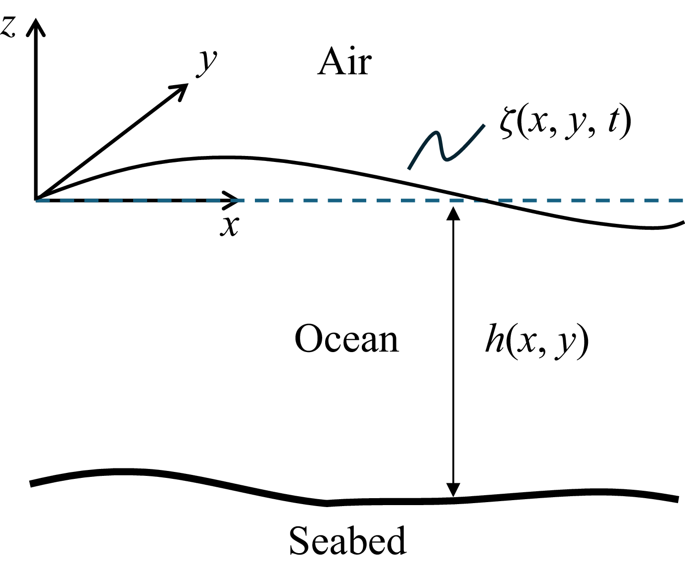
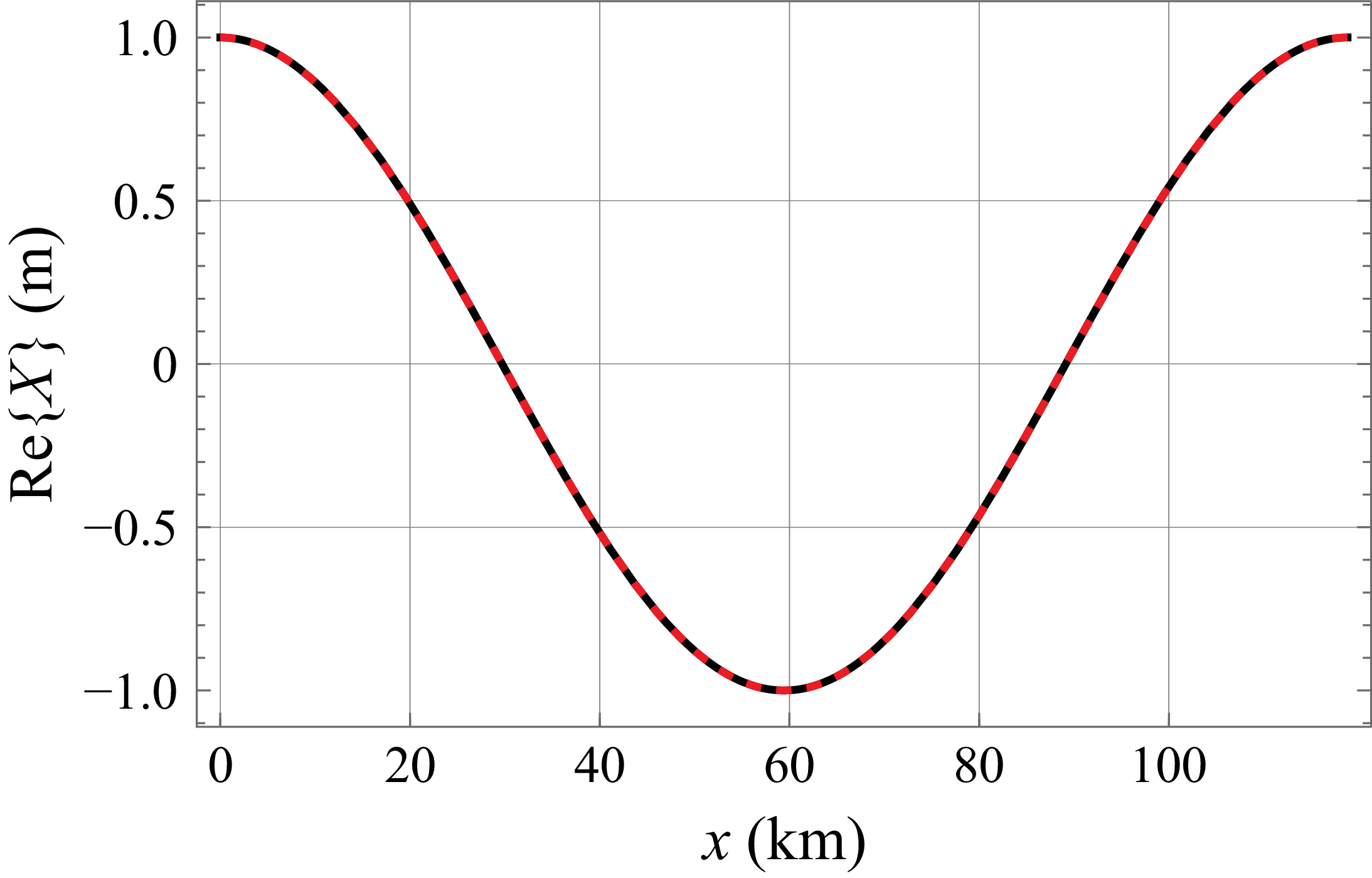


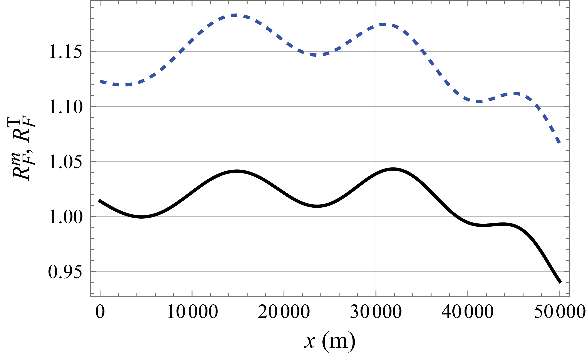


 Open access