


1. Introduction
Mushy layers are reactive porous materials formed due to morphological instability during solidification of multicomponent alloys (e.g. see reviews in Worster Reference Worster2000; Anderson & Guba Reference Anderson and Guba2020; Hitchen & Wells Reference Hitchen and Wells2025). In many settings, solidification modifies the buoyancy of the melt in the liquid pore space, which can then convect. Convection drives chemical transport through the porous layer, which can modify the material properties because the mushy layer is reactive (Worster Reference Worster1997; Anderson & Guba Reference Anderson and Guba2020). A striking example is the formation of solid-free channels, or chimneys. Convective flow generates a tendency for local disequilibrium and either dissolution or crystallisation of the solid matrix in different regions. This can drive a flow-focussing feedback where flow and solute transport preferentially focus in regions of high porosity and permeability, driving further dissolution (cf. Worster Reference Worster1997). In the natural environment, such convection drives chemical exchange between the porous interior of sea ice and the ocean, with implications for brine fluxes and ocean buoyancy forcing (Wettlaufer, Worster & Huppert Reference Wettlaufer, Worster and Huppert1997; Hunke et al. Reference Hunke, Notz, Turner and Vancoppenolle2011; Worster & Rees Jones Reference Worster and Rees Jones2015; Wells, Hitchen & Parkinson Reference Wells, Hitchen and Parkinson2019). Such convection may also be important for solute rejection during solidification of planetary inner cores (e.g. Bergman & Fearn Reference Bergman and Fearn1994; Huguet et al. Reference Huguet, Alboussiére, Bergman, Deguen, Labrosse and Lesœur2016). In industrial settings, the reactive flow focussing results in compositional heterogeneity and freckle defects in metal castings (Copley et al. Reference Copley, Giamei, Johnson and Hornbeck1970). In many such settings the solidification dynamics is inherently transient with the mushy layer growing over time, and may feature a range of initial alloy compositions. In Hitchen & Wells (Reference Hitchen and Wells2025), hereafter Part 1, we investigated how the cooling conditions and composition impact mushy-layer structure during diffusively controlled transient growth. The goal here is to understand the resulting impact on the onset of convection, using linear stability analysis as a tool to reveal dynamical insight.
Convection during steady growth (such as directional solidification of an alloy pulled between heat exchangers) has been widely studied using linear and weakly nonlinear stability analyses, fully nonlinear simulations and analogue experiments (see reviews by Worster Reference Worster1997; Wells et al. Reference Wells, Hitchen and Parkinson2019; Anderson & Guba Reference Anderson and Guba2020). Convection is observed when a mushy-layer Rayleigh number  $R_m={g\Delta \rho \varPi l }/{\kappa \mu }$ exceeds a critical value $R_c$. This Rayleigh number represents a ratio of buoyancy effects to dissipation, where $g$ is the gravitational acceleration, $\Delta \rho$ a characteristic density difference, $\varPi$ a permeability scale, $\kappa$ the thermal diffusivity, $\mu$ the dynamic viscosity with kinematic viscosity $\nu$ and for steady growth at rate $V$ we identify $l\sim {\kappa }/{V}$ with the diffusive length scale. The critical value of $R_m$ depends on the material properties and can also be modified by external flow (Neufeld & Wettlaufer Reference Neufeld and Wettlaufer2008a,Reference Neufeld and Wettlauferb), lateral confinement (Zhong et al. Reference Zhong, Fragoso, Wells and Wettlaufer2012) or other variation of growth conditions (see review by Anderson & Guba Reference Anderson and Guba2020). Of particular relevance here is the linear stability analysis of Worster (Reference Worster1992), which showed that decreasing the concentration ratio $\mathcal {C}={(\hat {S}_\infty -\hat {S}_s)}/{(\hat {S}_c-\hat {S}_\infty )}$ increases the critical Rayleigh number and wavenumber, where the initial fluid composition $\hat {S}_\infty$, the composition of pure solid $\hat {S}_s$ and $\hat {S}_c$ is the composition corresponding to the cooling boundary temperature (sometimes taken as the eutectic composition). Worster (Reference Worster1992) linked this to changes to the porosity and permeability of the layer causing flow confinement, showing that a compensated Rayleigh number $\overline {R_m}$ with permeability $\varPi$ evaluated at the mean depth-averaged porosity and length scale $l$ corresponding to the mush thickness results in $\overline {R_m}\sim 5\unicode{x2013}10$ for $0.1\leq \mathcal {C} \leq 10$. A similar magnitude was obtained with variation of the liquid superheat and Stefan number, where the latter characterises the ratio of latent and specific heats. Chen, Lu & Yang (Reference Chen, Lu and Yang1994) find that small values of $\mathcal {C}$ lead to stronger convection in the compositional boundary layer in the liquid adjacent to the mush.
The concept of a critical Rayleigh number for convection broadly extends to transient growth from cold isothermal boundaries with fixed chill. Experiments with a range of compositions are consistent with the emergence of chimneys and mushy-layer convection when the mush thickness  $\hat {h}$ exceeds a critical value $\hat {h}_c$ (e.g. Bergman & Fearn Reference Bergman and Fearn1994; Chen et al. Reference Chen, Lu and Yang1994; Chen Reference Chen1995; Wettlaufer et al. Reference Wettlaufer, Worster and Huppert1997) Since the mush thickness $\hat {h}(\hat {t})$ grows over time $\hat {t}$, this can also be interpreted as a critical time scale for convective onset, when the Rayleigh number based on a length scale $l=\hat {h}(\hat {t})$ exceeds a critical value. This interpretation potentially obscures changes to the interior structure of the mushy layer. Aussillous et al. (Reference Aussillous, Sederman, Gladden, Huppert and Worster2006) and Notz & Worster (Reference Notz and Worster2009) measured porosity during growth for certain concentration conditions, with results consistent with a spatial confinement of the convective flow to a high permeability region near the mush–liquid interface. Using scaling arguments they interpret this in terms of a local Rayleigh number $R_m\approx R_c$ based on $\Delta \rho$, $\varPi$ and $l$ evaluated over the vertical scale of the convecting cells. Variations of these arguments underpin various parameterisations of the convective desalination of sea ice (see review by Worster & Rees Jones Reference Worster and Rees Jones2015) which motivates understanding their theoretical underpinnings and how they should extrapolate across a range of growth conditions.
A number of previous linear stability analyses have considered development of convection during transient growth, with composition in a near-eutectic limit (cf. Emms & Fowler Reference Emms and Fowler1994) where the porosity remains of order one throughout the depth of the mushy layer. Using a quasi-steady stability analysis, which considers growth or decay of convective perturbations relative to the instantaneous background state at time  $\hat {t}$, Emms & Fowler (Reference Emms and Fowler1994) find convection above a critical Rayleigh number, where the length scale $l\propto \sqrt {\kappa \hat {t}}$ is interpreted in terms of the growing mush thickness. The critical Rayleigh number increases between 9 and 25 as the superheat increases. Using a propagation method, where perturbations are restricted to grow in the self-similar coordinates of the background state Hwang & Choi (Reference Hwang and Choi2000) considered a near-eutectic limit, neglecting the feedback of porosity on permeability. The results approach those of Emms & Fowler (Reference Emms and Fowler1994) for large superheat, but result in greater stability (i.e. larger critical Rayleigh number) than found by Emms & Fowler (Reference Emms and Fowler1994). Because the propagation method restricts the range of allowed perturbations, it has previously been found to overestimate stability bounds for Rayleigh–Darcy convection in a uniform porous medium (see discussion in Tilton, Daniel & Riaz Reference Tilton, Daniel and Riaz2013), which may explain this discrepancy. Subsequent studies using the propagation method considered the boundary-layer mode of convection when there is a diffusive boundary layer in the neighbouring liquid (Hwang & Choi Reference Hwang and Choi2004), while Hwang & Choi (Reference Hwang and Choi2008) characterised how the resulting time scale varies with superheat, and Hwang & Choi (Reference Hwang and Choi2009) show that the critical Rayleigh number is reduced by use of the Beavers & Joseph (Reference Beavers and Joseph1967) boundary condition for flow at the boundary between liquid and porous regions. Hwang (Reference Hwang2013) included the feedback of porosity on permeability, and used the propagation method to show that the critical Rayleigh number and wavenumber both decrease as either $\mathcal {C}$ or the superheat increases. A link to convective confinement was suggested, but not quantitatively explored.
The goal of this study is to systematically evaluate how the material structure of a transiently growing mushy layer impacts the onset of convection, using linear stability analysis to provide insight into the key mechanisms. We first consider the impact on convective onset of material composition and thermal parameters for fixed-chill cooling with an upper isothermal boundary. We then evaluate the effect of imperfect cooling with a more general Robin boundary condition, where the surface heat flux is linearly related to the surface temperature. The latter yields a more realistic linearised approximation to the surface energy balance during sea-ice growth (Hitchen & Wells Reference Hitchen and Wells2016). The relative efficiency of boundary cooling vs conduction through the mush is characterised by a dimensionless Biot number, which increases over time proportional to the diffusion length  $\sqrt {\kappa \hat {t}}$. Using a quasi-steady stability analysis we find that convection in fixed-chill conditions is strongly stabilised for compositions in the so-called Stefan limit (cf. Part 1) with $\mathcal {C} \ll 1$, with the critical Rayleigh number and wavenumber increasing as the concentration ratio $\mathcal {C}$ decreases. We demonstrate this change in stability is quantitatively consistent with a local Rayleigh number across a region of convective confinement, providing theoretical support for the scaling arguments of Aussillous et al. (Reference Aussillous, Sederman, Gladden, Huppert and Worster2006) and Notz & Worster (Reference Notz and Worster2009). Imperfect cooling can either inhibit or promote the onset of convection, with the global critical Rayleigh number first decreasing then increasing as the Biot number decreases. We interpret the results in terms of a tendency for full-depth convective disturbances if buoyancy forcing is large enough to trigger convection at early times when most of the mush has high porosity. At later times, any convection localises in a higher porosity region at the base of the ice, approaching behaviour consistent with the fixed-chill limit at large times.
The article is organised as follows. Section 2 describes the relevant model equations for flow in a transiently growing mushy layer, and § 3 describes the linearisation and solution method. Results with a fixed-chill boundary are described in § 4, whilst § 5 considers the Robin condition with imperfect boundary cooling. Section 6 discusses implications for sea-ice growth in the environment, and conclusions are summarised in § 7.
2. Model
Building on the model presented in Part 1, we study a binary alloy exposed at dimensionless time  $t=0$ to a heat sink at dimensionless depth $z=0$, with heat loss via a linearised exchange defined below. We neglect salt diffusion and assume the mushy layer is ideal with equal material properties in each phase. We further assume that the fluid is initially of uniform temperature and salinity, and that the initial velocity is uniformly zero. However, for this part, we will focus our attention on the growing mushy layer specifically and relax the assumption that the fluid always stays at rest.
For brevity, we skip the dimensional form of the model described in Part 1 and non-dimensionalise initially using a fixed, time-independent length scale,  $\hat {d}$, but convert to a scale defined by the thermal diffusion length scale later in the analysis. The initial length scale has associated time and velocity scales, ${\hat {d}^2}/{\kappa }$ and ${\kappa }/{\hat {d}}$, respectively. A diagram of the non-dimensional system is shown in figure 1.

Figure 1. Non-dimensional model set-up (cf. dimensional form in figure 1 in Part 1). The temperature profile  $\theta$ runs between $0$ at the surface heat sink and $\theta _{\infty }$ at depth, while the liquid salinity $S=1$ and its liquidus temperature is ${\theta }_L=1$. The thermal diffusion length scale is proportional to $\sqrt {t}$ and the constant of proportionality for linearised heat transfer is ${\mathcal {B}_i}$. A full description of the non-dimensional parameters used can be found in the main text.
The non-dimensional temperature and salinity are defined as
 \begin{equation} \theta = \frac{T - T_c}{T_{L\infty} - T_c},\quad S = \frac{\hat{S}-\hat{S}_s}{\hat{S}_\infty-\hat{S}_s}, \end{equation}
for dimensional temperature  $T$ and salinity $\hat {S}$. The temperature scale used $\Delta T = T_{L\infty } - T_c$ is the temperature difference between the salinity-dependent freezing temperature of the liquid $T_{L\infty }$ and the surface heat sink at $T_c$. The salinity scale used is the initial difference between the liquid salinity $\hat {S}_\infty$ and pure solid salinity $\hat {S}_s$.
Under this non-dimensionalisation, conservation of energy and salt yields
 \begin{equation} \frac{\partial{\theta}}{\partial{t}} + \boldsymbol{u}\boldsymbol{\cdot}\boldsymbol{\nabla}\theta + {\mathcal{S}_t}\frac{\partial{\chi}}{\partial{t}} = \nabla^2\theta,\quad \frac{\partial{\chi S}}{\partial{t}} =- \boldsymbol{u}\boldsymbol{\cdot}\boldsymbol{\nabla}S, \end{equation}
where we have added advective terms to the equations presented in Part 1 with Darcy velocity  $\boldsymbol {u}$ describing the volume flux of liquid per unit area. These equations introduce the volumetric liquid fraction $\chi$, and the Stefan number ${\mathcal {S}_t} = {L}/{c_p(T_{L\infty }-T_c)}$ which represents the ratio of latent heat $L$ to specific heat in the system (with specific heat capacity $c_p$). The temperature and salinity are constrained to each other via the liquidus relationship
 \begin{equation} \theta = 1 - \mathcal{C}(S-1),\quad \mbox{where}\ \mathcal{C}= \frac{\varGamma(\hat{S}_\infty-\hat{S}_s)}{T_{L\infty} - T_c} \equiv \frac{\hat{S}_\infty-\hat{S}_s}{\hat{S}_c-\hat{S}_\infty}, \end{equation}
where  $\hat {S}_c$ is the salinity of fluid with liquidus temperature $T_c$ and $\varGamma$ is the dimensional liquidus slope. The dimensionless concentration ratio $\mathcal {C}$ measures the salinity effects due to freezing-point depression, with a larger value indicating a larger impact on the solidification dynamics.
To complete the set of dynamic equations, we use Darcy's law to describe momentum transfer within the porous mush, and note that the fluid is incompressible when solid and liquid densities are assumed equal, yielding
 \begin{equation} \boldsymbol{u} =-\mathcal{R}_{m}\chi^3[\boldsymbol{\nabla}p + \theta\boldsymbol{{e_z}}],\quad \boldsymbol{\nabla}\boldsymbol{\cdot}\boldsymbol{u} = 0,\quad \mathcal{R}_{m} = \frac{g (\alpha + {\beta}/{\varGamma}) \Delta T\hat{\varPi}_0\hat{d}}{\kappa\nu}. \end{equation}
In the first of these equations,  $p$ is the dimensionless pressure, $\boldsymbol {{e_z}}$ is a vertical unit vector pointing downwards and we assume the permeability is $\hat {\varPi }_0\chi ^3$ for constant $\hat {\varPi }_0$, which approximates a measured correlation of sea-ice permeability ${\propto }\chi ^{3.1}$ (Freitag Reference Freitag1999; Notz & Worster Reference Notz and Worster2009). The density anomalies driving convection $\Delta \rho = \rho _0[ \beta (\hat {S}-\hat {S}_c) -\alpha (T -T_c)]$ are assumed to satisfy a linear equation of state with constant values of the thermal expansion coefficient $\alpha$, solutal contraction coefficient $\beta$ and reference density $\rho _0$. The liquidus relationship has been used to express saline buoyancy contributions in terms of the dimensionless temperature. The mushy Rayleigh number $\mathcal {R}_{m}$ describes the relative strength of buoyancy forcing from both thermal and saline expansion/contraction vs the rate of viscous and thermal dissipation.
Following Emms & Fowler (Reference Emms and Fowler1994) we treat the mush–liquid interface as an isothermal, constant-pressure boundary at the freezing temperature which yields
 \begin{equation} \theta = 1,\quad \boldsymbol{{e_x}}\boldsymbol{\cdot}\boldsymbol{u} = 0,\quad \text{when}\ {z = h}, \end{equation}
where  $\boldsymbol {{e_x}}$ is a horizontal unit vector and we have used (2.4a) to link $p$ and $\boldsymbol {u}$. Here, the isothermal condition arises from a marginal equilibrium condition, with the temperature satisfying the liquidus constraint with an assumed uniform salinity in the liquid. Note that the liquid fraction $\chi \rightarrow 1$ at the mush–liquid interface $z\rightarrow h$ in the background state. Emms & Fowler (Reference Emms and Fowler1994) justify use of a constant-pressure boundary condition when the resistance to flow in the liquid region is much smaller than in the porous region, which here occurs when the Darcy number $Da = \hat {\varPi }_0/\hat {d}^2$ is small.
Our treatment of the flow boundary conditions assumes a sharp transition between a pure liquid in  $z>h$ and a porous medium in $z< h$. Le Bars & Worster (Reference Le Bars and Worster2006) analysed the transition between purely liquid and porous regions using the Darcy–Brinkmann equation. They found that a split-domain approach with Navier–Stokes and Darcy flow in separate regions is an accurate approximation if the flow boundary conditions at a mush–liquid interface are characterised by instead imposing continuity of pressure and velocity at a displaced dimensional distance $\hat {\delta }=\sqrt {\hat {\varPi }/\chi }$ inside the porous media, where $\hat {\varPi }$ is the dimensional permeability. Applying the permeability used in (2.4a–c) and noting $\chi \sim 1$ near the mush–liquid interface, this corresponds to a dimensionless distance of $\delta =O (Da^{1/ 2})$ from the interface. This displacement from the mush–liquid interface can be neglected whenever it is much smaller than the thickness of the convecting cells (requiring $Da^{1/ 2} \ll h$ for full-depth convection, or $Da^{1/ 2} \ll h\mathcal {C}$ if convection is confined to a fraction of order $\mathcal {C}$ of the full depth.
At the cooling boundary, we apply a linear thermal exchange and an impermeable condition
 \begin{equation} \frac{\partial{\theta}}{\partial{z}} = {\mathcal{B}_i}\theta,\quad \boldsymbol{{e_z}}\boldsymbol{\cdot}\boldsymbol{u} = 0,\quad \text{when}\ {z = 0}, \end{equation}
where the Biot number  ${\mathcal {B}_i} = \mathfrak{h}\hat {d}/k$ characterises the ratio of the effective thermal conductivity $\mathfrak {h}\hat {d}$ of the boundary vs the thermal conductivity $k$ of the mushy layer. The limit ${\mathcal {B}_i} \rightarrow \infty$ represents a perfectly conducting, isothermal, boundary (see Part 1 for further discussion).
We will focus on the development of perturbations in the mushy layer  $0< z< h$ using (2.1a,b)–(2.6a,b). However, the background state also depends on properties of the liquid region which has no flow $(\boldsymbol {u}=0)$, uniform salinity $S=1$ and temperature evolving according to (2.2a) with $\chi =1$ and $\theta \rightarrow \theta _{\infty }$ as $z\rightarrow \infty$. Here, the dimensionless far-field temperature of the liquid $\theta _{\infty }={(T_\infty -T_c)}/{(T_{L\infty }-T_c)}$, with $\theta _{\infty }=1$ indicating fluid is at the liquidus temperature for salinity $\hat {S}_\infty$, and $\theta _{\infty }$ increases with the far-field liquid temperature. This parameter and its effects on the dynamics are discussed further in Part 1.
3. Stability method
We use a frozen time stability method (also known as a quasi-static stability analysis) to find the linear stability criteria of the mushy layer in various parameter configurations. This neglects nonlinear products of the perturbations to the base state, and assumes that the base state evolves at a much slower rate than the perturbation time scale, such that the base state can be considered static, or ‘frozen’.
Assuming a two-dimensional convection pattern, incompressibility (2.4b) is satisfied by writing  $\boldsymbol {u} = \boldsymbol {\nabla }\times (\psi \boldsymbol {{e_y}})$ using a streamfunction $\psi$ and unit vector $\boldsymbol {{e_y}}$ perpendicular to the plane. This results in a system with three fields, which are expanded as base states and perturbations
 \begin{equation} \theta = {\theta}_B(z,t) + \epsilon {\theta}_p(x,z,t),\quad \chi= {\chi}_B(z,t) + \epsilon {\chi}_p(x,z,t),\quad \psi = \epsilon \psi_p(x,z,t), \end{equation}
where  $\epsilon$ is the small perturbation amplitude and the base-state streamfunction is uniformly zero. The base-state equations of $O(1)$ yielded by this substitution are those solved in Part 1 for diffusive growth, while the linear perturbation equations found by gathering terms of $O(\epsilon )$ are
 \begin{gather} \frac{\partial{{\theta}_p}}{\partial{t}} + \frac{\partial{{\theta}_B}}{\partial{z}}\frac{\partial{\psi_p}}{\partial{x}} + {\mathcal{S}_t}\frac{\partial{{\chi}_p}}{\partial{t}} = \nabla^2{\theta}_p, \end{gather}
 \begin{gather}-\mathcal{R}_{m}\frac{\partial{{\theta}_p}}{\partial{x}} = \boldsymbol{\nabla}\boldsymbol{\cdot}\left[\frac{1}{{{\chi}_B}^3}\boldsymbol{\nabla}\psi_p\right], \end{gather}
 \begin{gather}(\mathcal{C} + 1-{\theta}_B)\frac{\partial{{\chi}_p}}{\partial{t}} - {\theta}_p\frac{\partial{{\chi}_B}}{\partial{t}} - {\chi}_p\frac{\partial{{\theta}_B}}{\partial{t}} - {\chi}_B\frac{\partial{{\theta}_p}}{\partial{t}} = \frac{\partial{{\theta}_B}}{\partial{z}}\frac{\partial{\psi_p}}{\partial{x}}, \end{gather}
where (3.2b) arises from rearranging Darcy's law (2.4a) and taking the curl. We decompose into Fourier modes with wavenumber  $\mathrm {k}$ and exponential growth rate $\sigma$
 \begin{equation} \left[\begin{array}{c} {\theta}_p(x,z,t)\\ \psi_p(x,z,t)\\ {\chi}_p(x,z,t) \end{array}\right]= \left[\begin{array}{c} {\theta}_f(\mathrm{k},z)\\ {\rm i}\mathrm{k}\psi_f(\mathrm{k},z)\\ {\chi}_f(\mathrm{k},z) \end{array}\right] {\rm e}^{{\rm i}\mathrm {k}x}\,{\rm e}^{\sigma t}, \end{equation}
with (3.2) yielding a matrix eigenvalue problem for either  $\sigma$ or $\mathcal {R}_{m}$
 \begin{gather} {\textit{A}}\boldsymbol{y} - \mathcal{R}_{m} {\textit{B}}\boldsymbol{y} = \sigma{\textit{C}}\boldsymbol{y}, \end{gather}
 \begin{gather}\boldsymbol{y} =
\left[\begin{array}{@{}c@{}} {\theta}_f \\ \psi_f \\ {\chi}_f
\end{array}\right],\quad {\textit{A}}
=\left[\begin{array}{@{}ccc@{}} \partial^2/\partial z^2 -
\mathrm{k}^2 & \mathrm{k}^2 {\partial
{{\theta}_B}}/{\partial {z}} & 0\\ 0 &
\dfrac{\partial{}}{\partial{z}}\left(\dfrac{1}{{{\chi}_B}^3}\dfrac{\partial{}}{\partial{z}}\right)
- \dfrac{\mathrm{k}^2}{{{\chi}_B}^3} & 0\\ -{\partial
{{\chi}_B}}/{\partial {t}} & \mathrm{k}^2{\partial
{{\theta}_B}}/{\partial {z}} & -{\partial
{{\theta}_B}}/{\partial {t}} \end{array}\right],
\end{gather}
\begin{gather}\boldsymbol{y} =
\left[\begin{array}{@{}c@{}} {\theta}_f \\ \psi_f \\ {\chi}_f
\end{array}\right],\quad {\textit{A}}
=\left[\begin{array}{@{}ccc@{}} \partial^2/\partial z^2 -
\mathrm{k}^2 & \mathrm{k}^2 {\partial
{{\theta}_B}}/{\partial {z}} & 0\\ 0 &
\dfrac{\partial{}}{\partial{z}}\left(\dfrac{1}{{{\chi}_B}^3}\dfrac{\partial{}}{\partial{z}}\right)
- \dfrac{\mathrm{k}^2}{{{\chi}_B}^3} & 0\\ -{\partial
{{\chi}_B}}/{\partial {t}} & \mathrm{k}^2{\partial
{{\theta}_B}}/{\partial {z}} & -{\partial
{{\theta}_B}}/{\partial {t}} \end{array}\right],
\end{gather} \begin{gather}{\textit{B}} =
\left[\begin{array}{@{}ccc@{}} 0 & 0 & 0\\ -1 & 0 & 0\\ 0 & 0 & 0
\end{array}\right],\quad {\textit{C}}
=\left[\begin{array}{@{}ccc@{}} 1 & 0 & {\mathcal{S}_t}\\ 0 & 0 &
0\\ {\chi}_B & 0 & -(\mathcal{C} + 1-{\theta}_B)
\end{array}\right].
\end{gather}
\begin{gather}{\textit{B}} =
\left[\begin{array}{@{}ccc@{}} 0 & 0 & 0\\ -1 & 0 & 0\\ 0 & 0 & 0
\end{array}\right],\quad {\textit{C}}
=\left[\begin{array}{@{}ccc@{}} 1 & 0 & {\mathcal{S}_t}\\ 0 & 0 &
0\\ {\chi}_B & 0 & -(\mathcal{C} + 1-{\theta}_B)
\end{array}\right].
\end{gather}
For computational efficiency, the results below solve the problem directly for the critical Rayleigh number by assuming  $\sigma = 0$ at the exchange of stability. Setting $\sigma = 0$ has the effect of making the stability independent of perturbations to the liquid fraction, because (3.4) decouples into a $2\times 2$ matrix eigenvalue problem for ${\theta }_f$ and $\psi _f$ with ${\chi }_f$ decoupled and determined from ${\theta }_f$ and $\psi _f$. However, this also explicitly neglects oscillatory modes from the calculation, with $\Im \{\sigma \} \neq 0$. Oscillatory modes contained within the mushy region have previously been found for models with asymptotically thin mushy layers in the near-eutectic limit (see Anderson & Worster Reference Anderson and Worster1996; Anderson & Guba Reference Anderson and Guba2020), but usually have a relatively minor impact on the critical Rayleigh number for instability. For example, the results illustrated by Anderson & Worster (Reference Anderson and Worster1996) show changes of ${\lesssim }20\,\%$ to the critical Rayleigh number for convective onset when oscillatory modes are the most unstable.
Applying the same decomposition to the boundary conditions leads to
 \begin{gather} \frac{\partial{{\theta}_f}}{\partial{z}} = {\mathcal{B}_i}{\theta}_f,\quad \psi_f =0,\quad \text{at}\ {z=0}, \end{gather}
 \begin{gather}{\theta}_f =0,\quad \frac{\partial{\psi_f}}{\partial{z}} =0,\quad \text{at}\ {z=h}, \end{gather}
where for simplicity we have neglected deformation of the mush–liquid interface and assumed no perturbations to  $h$. In an analysis of asymptotically thin mushy layers in the near-eutectic limit, Roper, Davis & Voorhees (Reference Roper, Davis and Voorhees2008) showed this assumption does not qualitatively impact the stability results, and only leads to a modest quantitative difference in the critical $\mathcal {R}_{m}$ by ${\lesssim }10\,\%$.
Time now only appears in (3.4) and (3.5) through the base-state temperature and liquid fraction,  ${\theta }_B$ and ${\chi }_B$, but we showed in Part 1 that these profiles can be calculated in self-similar coordinates using the variables $\tilde z$ and ${\tilde {\mathcal {B}}_i}$. We therefore repeat the same self-similarity transformation
 \begin{gather} \tilde z = \frac{z}{\sqrt{t}},\quad \tilde{\mathrm{k}} = \mathrm{k} \sqrt{t},\quad \lambda = \frac{h}{\sqrt{t}}, \end{gather}
 \begin{gather}\tilde{\mathcal{R}}_{m} =\mathcal{R}_{m} \sqrt{t},\quad {\tilde{\mathcal{B}}_i} = {\mathcal{B}_i} \sqrt{t},\quad \tilde{\theta} =\theta,\quad \tilde\psi_f = \frac{\psi_f}{\sqrt{t}}, \end{gather}
which we noted is equivalent to changing the length scale of the problem from the fixed length  $\hat {d}$ to the time-evolving thermal diffusion length scale $\sqrt {\kappa \hat {t}}$. This transformation leaves the decoupled, $2\times 2$ form of (3.4) and (3.5) unchanged.
Finally, we note that varying parameters such as the far-field liquid temperature and Stefan number will change the depth of the mushy layer. This changing vertical extent will have a well-understood impact on the convective instability, with the critical Rayleigh number varying in inverse proportion to the layer depth. To allow us to see past this effect, it is useful to define the scaled Rayleigh number and the corresponding wavenumber
 \begin{equation} \tilde{\mathcal{R}}_{m}^* = \lambda\tilde{\mathcal{R}}_{m} = \frac{g(\alpha+ {\beta}/{\varGamma})\Delta T\hat{\varPi}_0\hat{h}(\hat{t})}{\kappa\nu} = \frac{\hat{h}(\hat{t})}{\hat{d}_m},\quad \tilde{\mathrm{k}}^* = \tilde{\mathrm{k}} \lambda = \hat{\mathrm{k}} \hat{h}(\hat{t}), \end{equation}
where  $\lambda =h(t)/\sqrt {t}$ is the self-similar interface position and the convective length scale $\hat {d}_m=\kappa \nu /[g(\alpha +{\beta }/{\varGamma })\Delta T \hat {\varPi }_0]$. In an experiment or application, the scaled Rayleigh number in (3.7a) will typically increase over time as the mushy layer grows and $\hat {h}$ increases. Our goal is to find the critical threshold value of $\tilde {\mathcal {R}}_{m}^*$ for the onset of instability as a function of the growth conditions that control the structure of the mushy layer, and also as a function of ${\tilde {\mathcal {B}}_i}$ which increases with time when there is imperfect boundary cooling. One can then infer a critical mush thickness or critical onset time for convection by inverting (3.7a) for $\hat {h}$ or $\hat {t}$.
The resulting eigenvalue system is discretised on a Chebyshev grid (see Trefethen Reference Trefethen2000) using between 60 and 200 nodes until the results are well converged. Following the method in Hitchen & Wells (Reference Hitchen and Wells2016) we rewrite the discretised boundary conditions as a constraint on the internal points. The critical  $\mathcal {R}_{m}$ is found at a range of wavenumbers using the Matlab ‘eig’ routine, and minimised to find the global stability point for that set of parameters.
4. Results for a perfectly conducting boundary
4.1. Impact of the concentration ratio on stability
The first part of our investigation focuses on the effect of the concentration ratio  $\mathcal {C}$ on the convective instability. After decoupling the third row of the matrix problem, the concentration ratio $\mathcal {C}$ does not appear in either (3.4) or (3.5) explicitly, but does affect the internal structure of the base state ${\theta }_B$ and ${\chi }_B$. We aim to see how the changes to the internal structure controlled by $\mathcal {C}$ impact the stability of the mushy layer. Varying $\mathcal {C}$ will also affect the growth rate, but we will use the scaled Rayleigh number, $\tilde {\mathcal {R}}_{m}^*$, which already accounts for the impact of the growth rate. The mushy layer is highly porous throughout for large values of $\mathcal {C}$ (see Part 1), with $\chi \rightarrow 1$ as $\mathcal {C} \rightarrow \infty$. In contrast, for small values of $\mathcal {C}$, we found that most of the mush has a very low liquid fraction with a small interfacial boundary layer containing most of the porosity variation. The far-field temperature used in this section will be $\theta _{\infty }=1.25$ unless stated otherwise, which for applications to sea ice corresponds roughly to Arctic ocean water with $\hat {S}_\infty =35\ \mathrm {g}\ \mathrm {kg}^{-1}$ at $0\,^{\circ }$C being cooled to $-10\,^{\circ }$C. In this section we will assume perfect boundary conductivity, ${\tilde {\mathcal {B}}_i}\rightarrow \infty$.
Figure 2 shows the variation of the critical scaled Rayleigh number and wavenumber as the concentration ratio and Stefan number are varied. Detailed discussion of the dependence on Stefan number will be deferred until § 4.2. As the concentration ratio is decreased, there is a sharp increase in both the critical Rayleigh number  $\tilde {\mathcal {R}}_{m}^*$ (by several orders of magnitude) and wavenumber $\mathrm {k}_{c}^*$ (by one order of magnitude). The variation of $\tilde {\mathcal {R}}_{m}^*$ and $\mathrm {k}_{c}^*$ with ${\mathcal {S}_t}$ is much weaker. These increases of $\tilde {\mathcal {R}}_{m}^*$ and $\mathrm {k}_{c}^*$ with decreasing $\mathcal {C}$ are well described by the trends
 \begin{equation} \tilde{\mathcal{R}}_{m}^* \approx 39 + \frac{19}{\mathcal{C}^2},\quad \mathrm{k}_{c}^* \approx 2.4 + \frac{0.34}{\mathcal{C}}, \end{equation}
which are illustrated in figure 3(a,b) for  $\theta _{\infty }=1.25$ with varying $\mathcal {C}$ and ${\mathcal {S}_t}$, and in figure 3(c,d) for ${\mathcal {S}_t}=1$ with varying $\mathcal {C}$ and $\theta _{\infty }$. These trends are approximations which are independent of Stefan number. However, they provide a good match to the data across a range of ${\mathcal {S}_t}$ and $\mathcal {C}$ for $\theta _{\infty }=1.25$, and the maximum error of the Rayleigh number trend is $59.0\,\%$ with a root-mean-square error of $26.8\,\%$, while the maximum error of the wavenumber trend is $23.3\,\%$ with a root-mean-square error of $4.1\,\%$ for the parameter values in figure 3(a,b). We later present explanations for these scalings and their dependence on $\mathcal {C}$ and $\theta _{\infty }$.

Figure 2. (a) Scaled critical Rayleigh numbers  $\tilde {\mathcal {R}}_{m}^*$ against concentration ratio $\mathcal {C}$ and Stefan number ${\mathcal {S}_t}$, calculated when $\theta _{\infty }=1.25$. The black contours are spaced at intervals of $10^{0.2}$ and the green contours are at $\tilde {\mathcal {R}}_{m}^*=36$, $37$,
$37$,  $38$ and $39$. The critical Rayleigh number increases sharply as the concentration ratio is decreased, as discussed in the main text. (b) The corresponding critical wavenumbers $\mathrm {k}_{c}^*$ over the same range of concentration ratio and Stefan number. The black contours are now at intervals of $10^{0.1}$ and the green contours are $\mathrm {k}_{c}^*=2.4$ and $2.45$. The wavenumber also increases as the concentration ratio decreases. Note reversed scales on logarithmically spaced colour bars.

Figure 3. (a) Critical Rayleigh numbers  $\tilde {\mathcal {R}}_{m}^*$ and (b) critical wavenumbers against concentration ratio $\mathcal {C}$, for Stefan numbers in the range $0.0125 \leq {\mathcal {S}_t} \leq 1250$ and $\theta _{\infty }=1.25$, calculated in coordinates scaled such that the depth of the mushy layer is 1. The upper and lower bounds of the data for varying ${\mathcal {S}_t}$ are shown in orange and green, respectively, while the dashed black curves are given by equation (4.1a,b) (where the numerical constants have been determined to minimise the sum of relative errors over all data points, using MATLAB function ‘fminsearch’). (c) Shows corresponding variation of the critical Rayleigh number $\tilde {\mathcal {R}}_{m}^*$ vs $\mathcal {C}$, and (d) wavenumber vs $\mathcal {C}$ for varying $\theta _{\infty }$ and ${\mathcal {S}_t}=1.25$, illustrating that (4.1a,b) captures the leading-order trend for a range of $\theta _{\infty }$ and ${\mathcal {S}_t}$.
Our results echo those of Hwang (Reference Hwang2013), which were obtained using the propagation method that assumes self-similar perturbations. Hwang (Reference Hwang2013) observed a large increase in Rayleigh number and a moderate increase in wavenumber as the concentration ratio  $\mathcal {C}$ decreases below $1$, with both tending to a constant value for large values of $\mathcal {C}$. Hwang (Reference Hwang2013) hypothesises that this behaviour is due to the presence of a low-porosity region for small $\mathcal {C}$ which confines the convection, but does not investigate this further. To investigate this phenomenon, figure 4 shows the convection, liquid fraction and permeability profiles for three different values of the concentration ratio. In figure 4(a), $\mathcal {C} = 3.8$ and $\theta _{\infty } = 1.25$, corresponding to the high-liquid-fraction regime $(\mathcal {C}\gg 1)$ with $\chi >0.79$ throughout the depth, and high permeability ( $\varPi \equiv \chi ^3>0.49$). In this regime, the convection penetrates the full depth of the mushy layer and the cells are relatively wide with width of comparable magnitude to the thickness of the layer. Figure 4(b) shows results for $\mathcal {C}=0.38$ in the transitional regime with appreciable solid formation close to the upper boundary ( ${\chi }_B(0) = 0.27$). This is reflected in the convection pattern with the convection confined further away from the upper boundary than in figure 4(a), and focussed more in the lower part of the domain. The convective cells also narrow slightly relative to the layer thickness. Finally, figure 4(c) shows results for
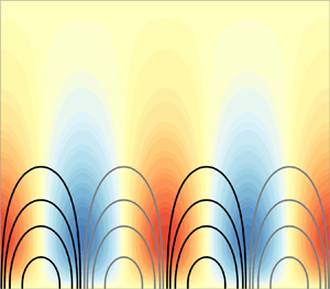
  $\mathcal {C}=0.038$ in the earlier-defined Stefan regime. Here, the top of the mushy layer has a large solid fraction and a low permeability, while the high-porosity mush is focused in a thin interfacial region. The convective cells are heavily confined to this interfacial region, and there is very little fluid motion in the rest of the domain, although thermal variations do spread slightly further than the velocity. Figure 5 shows the corresponding linear perturbations to the liquid fraction for the same parameter values as figure 4. The liquid fraction increases in regions of downward flow (see blue shaded regions in figure 5), consistent with downward advection of higher salinity pore fluid causing local dissolution of the solid matrix. The opposite trend is observed in regions of upward flow, with the comparatively fresh inflow causing local solidification and a reduction in liquid fraction.

Figure 4. (Left) Background liquid fraction and permeability profiles – blue and green curves, respectively – for  $\theta _{\infty }=1.25$, ${\mathcal {S}_t} = 0$ and (a) $\mathcal {C}=3.8$, (b) $\mathcal {C}=0.38$ and (c) $\mathcal {C}=0.038$. (Right) Marginally stable modes at $\tilde {\mathcal {R}}_{m}^*$ for the three cases. The thermal perturbations ${\theta }_p$ are shown by the colour scale. Streamfunction contours are shown at $0.02$, $0.05$, $0.1$, $0.2$ and $0.3$, with black contours representing clockwise circulation and grey contours representing anti-clockwise circulation.

Figure 5. Illustration of liquid-fraction perturbations and flow for the same marginally stable modes as shown in figure 4. (Left) Background liquid fraction and permeability profiles, as in figure 4, for  $\theta _{\infty }=1.25$, ${\mathcal {S}_t} = 0$ and (a) $\mathcal {C}=3.8$, (b) $\mathcal {C}=0.38$ and (c) $\mathcal {C}=0.038$. (Right) Marginally stable modes at $\tilde {\mathcal {R}}_{m}^*$ for the three cases, with liquid-fraction perturbations ${\chi }_p$ shown by the colour scale, and the same streamfunction contours as in figure 4 with black contours representing clockwise circulation and grey contours representing anti-clockwise circulation. Note that the amplitude of the perturbations in any physical realisation will be subject to a linear rescaling by the initial perturbation amplitude.
As a measure of this convective confinement, we calculate the  $z$-value at which the streamfunction drops below $10\,\%$ of its maximum value, and define the confinement depth $c_\lambda$ as the resulting distance from the mush–liquid interface divided by the mush thickness. We also calculate the liquid fraction at the confinement depth (confinement liquid fraction, $c_{\chi }$) and fraction of the temperature range which lies between the confinement depth and the mush–liquid interface (confinement temperature, $c_\theta = 1 - \theta |_{c_\lambda }$). These three diagnostic properties are shown in figure 6 for a range of concentration ratios and two Stefan numbers.

Figure 6. The confinement depth  $c_\lambda$ (blue), confinement liquid fraction $c_{\chi }$ (green) and confinement temperature $c_\theta$ (red) are plotted against the concentration ratio $\mathcal {C}$, for $\theta _{\infty }=1.25$ and two values of the Stefan number, ${\mathcal {S}_t} = 0$ (solid) and ${\mathcal {S}_t} = 15.7$ (dashed). Also shown in dotted grey line is the one-to-one trend line consistent with a scaling proportional to $\mathcal {C}$. The method of calculation for these properties is described in the main text.
For large values of the concentration ratio, the confinement depth tends to a value close to one, which represents convection through the full depth (by definition,  $c_\lambda$ will not reach one since $\psi = 0$ at the surface). For smaller values with $\mathcal {C}\ll 1$ in the Stefan regime, the confinement depth $c_\lambda$ varies approximately linearly with the concentration ratio, consistent with convection being confined to the high-porosity interfacial region of the mushy layer with a relative depth proportional to $\mathcal {C}$ as identified in Part 1. The confinement liquid fraction $c_{\chi }$ tends to a constant value as $\mathcal {C}$ decreases, with a limit of $\chi \approx 0.2$ for ${\mathcal {S}_t} = 0$ and $\chi \approx 0.3$ for ${\mathcal {S}_t} = 15.7$. Fluid motion is therefore being capped at the same liquid fraction for a large range of $\mathcal {C}$ and cannot substantially penetrate into the region of low liquid fraction which exists above this contour.
The scalings (4.1a,b) for the critical Rayleigh number and wavenumber can be understood as follows. The combination of a preference for convection cells to occur with a roughly square aspect ratio and the convective confinement to a region with a relative thickness  $l \propto \hat {h} \mathcal {C}$ for $\mathcal {C} \ll 1$ means that we expect a wavelength proportional to $\mathcal {C}$ when scaled relative to the mushy-layer thickness. Hence, the scaled critical wavenumber $\tilde {\mathrm {k}}^* =\hat {\mathrm {k}} \hat {h} \propto \hat {h}/l \propto {1}/{\mathcal {C}}$ for $\mathcal {C} \ll 1$, as seen in (4.1b). However, for $\mathcal {C} \gg 1$ there is negligible convective confinement and convection cells of order-one aspect ratio penetrate the full depth of the mushy layer, resulting in a wavelength comparable to $\hat {h}$ and scaled wavenumber $\tilde {\mathrm {k}}^* =\hat {\mathrm {k}} \hat {h} \sim \mathrm {constant}$. Equation (4.1b) recovers the scalings for each of these asymptotic limits.
The corresponding limits of (4.1a) can be reconciled by hypothesising that a local Rayleigh number evaluated over the depth of the convecting region  $\mathcal {R}_l \equiv g \Delta \rho _l l \varPi /\kappa \mu$ is approximately constant, where $\Delta \rho _l$ is the density difference driving convection. For $\mathcal {C} \gg 1$ convection penetrates the full mush depth with $l\sim \hat {h}$, whilst the density difference $\Delta \rho _l \sim \rho _0(\alpha +{\beta }/{\varGamma }) \Delta T$ depends on the imposed temperature drop across the mushy layer. Thus constant $\mathcal {R}_l$ implies that the scaled Rayleigh number $\tilde {\mathcal {R}}_{m}^* \sim \mathrm {constant}$ for $\mathcal {C} \gg 1$, consistent with the scaling of the corresponding limit of (4.1a). Meanwhile, for $\mathcal {C} \ll 1$, convective confinement restricts the active depth to $l \propto \hat {h} \mathcal {C}$, where the porosity is of order one and the permeability is of similar magnitude. To a first approximation, the temperature varies linearly with depth and hence the density difference over the length scale $l$ is a fraction $l/\hat {h}$ of the total across the mush, yielding $\Delta \rho _l \sim \rho _0(\alpha +{\beta }/{\varGamma }) \Delta T \mathcal {C}$. Combining these scales with a constant $\mathcal {R}_l$ implies the scaled Rayleigh number $\tilde {\mathcal {R}}_{m}^* \propto \mathcal {C}^{-2}$ for $\mathcal {C} \ll 1$, which is also consistent with the corresponding limit of (4.1a). Overall, the system is stabilised to convective disturbances with decreasing $\mathcal {C}$ because there is less potential energy available across the narrower high-porosity and high permeability region where convection can efficiently operate.
The results from this section can also be used to predict convective onset in terms of the convective length scale  $\hat {d}_m$ of the mushy layer. Combining (3.7a,b) and (4.1a,b), we find that convection with dimensional wavenumber $\hat {\mathrm {k}_{c}}$ starts when the mushy-layer thickness reaches the critical value
 \begin{equation} \hat{h} \approx\hat{d}_m\left(39 + \frac{19}{\mathcal{C}^2},\right),\quad \hat{\mathrm{k}_{c}} \approx\frac{2.4 + {0.34 }/{\mathcal{C} }}{ \hat{d}_m (39 + {19}/{\mathcal{C}^2 })}. \end{equation}
4.2. Effect of the Stefan number
We now consider the effect of varying the Stefan number  ${\mathcal {S}_t}$ on the stability of the mushy layer. The Stefan number characterises the amount of latent heat in the system, relative to the amount of specific heat. As with $\mathcal {C}$, ${\mathcal {S}_t}$ does not explicitly appear in the reduced eigenvalue problem (3.4) and (3.5) when solving for $\tilde {\mathcal {R}}_{m}^*$ with $\sigma = 0$, but will affect both ${\theta }_B$ and ${\chi }_B$.
In the high-liquid-fraction regime with  $\mathcal {C} \gg 1$ increasing the Stefan number results in a small, but noticeable, increase in the scaled Rayleigh number. This is shown in figure 7(a) for $\mathcal {C}=125$ where $\tilde {\mathcal {R}}_{m}^*$ increases by $2\,\%$ as ${\mathcal {S}_t}$ increases from approximately $0.01$ to $100$. With such a large concentration ratio, the porosity is greater than $0.99$ throughout the depth of the mushy layer regardless of Stefan number, but there are some modest changes to the base-state temperature profile for large Stefan numbers, as shown by the curvature of temperature contours in figure 7(b). As the Stefan number increases, more latent heat is released when solidification occurs and the effective heat capacity of the mushy layer is increased (cf. the simplified model in Part 1 with dimensionless effective heat capacity $\varOmega = 1 + {\mathcal {S}_t}/\mathcal {C}$). Fluid closer to the cooling boundary experiences a larger temperature change, more solidification and a greater release of latent heat than fluid further from the boundary. This results in slower thermal transport through the surface layer and less cooling further from the boundary, because the thermal energy cannot be removed as efficiently. The temperature profile therefore becomes less linear, with the gradient sharpening closer to the upper surface and flattening closer to the mush–liquid interface, as indicated by the upwards curve of temperature contours in figure 7(b) as they slightly compress near the upper boundary. Thermal forcing is proportional to the temperature gradient and hence is concentrated closer to the impermeable boundary at the upper surface, which is more restrictive on convective perturbations than the constant-pressure boundary at the interface (see discussion of boundary condition effects on convective stability in Hitchen & Wells (Reference Hitchen and Wells2016) for non-reactive porous media). This increases the boundary resistance experienced by the flow, and increases the scaled Rayleigh number.

Figure 7. (a) The scaled critical Rayleigh number against Stefan number for  $\mathcal {C} = 125$ and $\theta _{\infty } = 1.25$. Stefan numbers greater than one cause a small increase in the value of $\tilde {\mathcal {R}}_{m}^*$. (b) The corresponding base-state temperature profiles against Stefan number. The depth axis has been scaled by the mushy-layer depth to highlight changes in the vertical structure. For large Stefan numbers, the temperature contours curve slightly upwards.
By contrast, in the Stefan regime with  $\mathcal {C} \ll 1$ and low porosity over much of the depth, there is a decrease in scaled Rayleigh number by approximately one third as ${\mathcal {S}_t}$ increases from approximately $0.01$ to $100$, and the amount of latent heat in the system increases (figure 8a). Similarly to the high-liquid-fraction regime, the largest temperature gradients shift slightly upwards (not shown here), but this effect on the scaled Rayleigh number is relatively small compared with the changes that arise from the base-state liquid-fraction profile. Figure 8(b) shows a clear thickening of the high-porosity interfacial region as the Stefan number increases, which results from the warming of the mushy layer at depth following greater latent heat release. This decreases the scaled Rayleigh number because there is less resistance to flow over a greater range of depths at the base of the mushy layer.

Figure 8. (a) The scaled critical Rayleigh number against Stefan number for  $\mathcal {C} = 0.125$ and $\theta _{\infty } = 1.25$. Increasing the Stefan number causes an appreciable decrease in the value of $\tilde {\mathcal {R}}_{m}^*$. (b) The corresponding base-state liquid-fraction profiles against Stefan number, with black contours of constant $\chi$ spaced by $0.1$ for $0.2\leq \chi \leq 0.9$. Red curves represent (from the top down) $10\,\%$, $50\,\%$ and $90\,\%$ of the maximum streamfunction. Note that the $10\,\%$ contour is also used in the definition of the confinement depth, $c_\lambda$. The depth axis has been scaled by the mushy-layer depth to highlight changes in the internal structure. A larger Stefan number results in a larger high-porosity region close to the interface, with the streamfunction localising by increasing in the high-porosity region and decreasing for higher porosities.
However, the increased Stefan number also results in more localisation of the flow to within this enlarged high-porosity region. This can be seen in the streamfunction contours shown in figure 8(b), which reveal an interesting balance. There is a tradeoff between any increase in the vertical extent of a convection cell providing access to a larger temperature difference and more potential energy, but also increasing the resistance to flow from the lower porosity above. The trends of the streamfunction contours indicate this results in a distortion of convection cells with increasing  ${\mathcal {S}_t}$. At low ${\mathcal {S}_t}$ the convection cell expands comparatively deeply into the more resistive layer of lower porosity, in order to access sufficient potential energy to sustain convection. With increasing ${\mathcal {S}_t}$, the high-porosity region expands, allowing efficient access to more potential energy and the most intense convection penetrates further from the mush–liquid interface (cf. 90 % streamfunction contour in figure 8b). However, the overall thickness of the convecting region reduces slightly (cf. 10 % streamfunction contour) because the flow can access sufficient potential energy to maintain the flow without needing to propagate as far into the more resistive region of lower porosity. The increased localisation with increased Stefan number also manifests itself in figure 6 as a higher confinement liquid fraction and a lower confinement depth when the Stefan number is increased from $0$ to $12.6$.
5. Effect of imperfect boundary conduction
With an imperfectly conducting boundary, the solution depends on a rescaled Biot number  ${\tilde {\mathcal {B}}_i} = {\mathcal {B}_i} \sqrt {t}$ from (3.6) which also acts as a proxy for time. For deep porous layers of uniform porosity that are transiently cooled by an imperfectly conducting boundary, Hitchen & Wells (Reference Hitchen and Wells2016) found three ways that the Biot number could affect the convective stability: by changing the temperature range in the fluid, by changing the structure of the thermal forcing and by changing the boundary resistance applied to the thermal perturbation. For a mushy layer, the evolving Biot number will also affect the porosity of the mushy layer, with an initially high porosity throughout the mush depth, before porosities reduce as the Biot number ${\tilde {\mathcal {B}}_i} = {\mathcal {B}_i}\sqrt {t}$ grows (see Part 1). In this section, we investigate how these four effects impact the convective stability of a mushy layer, focussing on examples in both of the high-liquid-fraction and Stefan regimes.
For the high-liquid-fraction regime, we consider a system with  $\mathcal {C} = 12.5$, $\theta _{\infty } = 1.25$ and ${\mathcal {S}_t} = 125$. Such a system initially freezes with a Biot number of ${\tilde {\mathcal {B}}_i} = 0.21 \equiv {\tilde {\mathcal {B}}_f}$ and adjusts to reach a self-similar state for ${\tilde {\mathcal {B}}_i}\gtrsim 100$ at late times (see figure 6 in Part 1). There are significant changes to the growth rate, surface temperature and structure of the mushy layer as the effects of the cooling propagate through the system. Figure 9 shows that the scaled ‘global’ Rayleigh number $\tilde {\mathcal {R}}_{m}^*$, which is defined using the temperature range between the mush–liquid interface and the cooling heat sink and is given by (3.7a), initially decreases sharply with increasing ${\tilde {\mathcal {B}}_i}$ (e.g. increasing time), before reaching a plateau as the mush reaches the self-similar state at large time. The critical wavenumber increases with the Biot number (and with time). With imperfect thermal conduction from the boundary, the surface temperature evolves over time and the temperature difference across the mushy layer grows as ${\tilde {\mathcal {B}}_i}$ increases (figure 9c). To see the effects of this changing temperature difference, and to isolate it from structural and perturbation boundary condition changes, figure 9(a) also shows the evolution of a ‘local’ Rayleigh number
 \begin{equation} \tilde{\mathcal{R}}_{{m,l}}^*= \frac{g(\alpha+{\beta}/{\varGamma}) [T_{L\infty}-T(\hat{z}=0,\hat{t})]\hat{\varPi}_0\hat{h}}{\kappa\nu}, \end{equation}
defined using the temperature difference  $T_{L\infty }-T(\hat {z}=0,\hat {t})$ across the mushy layer only, rather than the temperature difference $\Delta T = T_{L\infty }-T_c$ between the mush–liquid interface and cooling heat sink. Here, hatted variables are dimensional. In contrast to the global Rayleigh number $\tilde {\mathcal {R}}_{m}^*$ (blue curve), the local Rayleigh number $\tilde {\mathcal {R}}_{{m,l}}^*$ (green curve) shows a modest increase with ${\tilde {\mathcal {B}}_i}$ and remains of similar order with $18.4\leq \tilde {\mathcal {R}}_{{m,l}}^* \leq 33.8$ for ${\tilde {\mathcal {B}}_f}\leq {\tilde {\mathcal {B}}_i} < \infty$. This indicates that the changing thermal range is the most significant effect of varying Biot number which increases over time. The global and local Rayleigh numbers converge for large ${\tilde {\mathcal {B}}_i}$ or late times, as the boundary approaches the temperature of the heat sink.

Figure 9. (a) Critical Rayleigh numbers, (b) critical wavenumbers and (c) temperature difference  $1 - \theta (\tilde z =0,{\tilde {\mathcal {B}}_i})$ across the mushy layer against Biot number for $\mathcal {C} = 12.5$, $\theta _{\infty } = 1.25$ and ${\mathcal {S}_t} = 125$. These conditions place the system well into the high-liquid-fraction regime, with $\chi >0.92$ for all ${\tilde {\mathcal {B}}_i}$. Two different definitions for the Rayleigh number are used. In blue is the ‘global’ Rayleigh number, $\tilde {\mathcal {R}}_{m}^*$ defined in (3.7a) in terms of the temperature difference from the mush–liquid interface to the temperature of the cooling heat sink and using the mushy-layer depth as the length scale. The ‘local’ Rayleigh number, $\tilde {\mathcal {R}}_{{m,l}}^*$, in green is defined in (5.1) using the temperature difference $1 - \theta (\tilde z =0,{\tilde {\mathcal {B}}_i})$ across the mushy layer only. Shown in dashed grey are the first solidification at ${\tilde {\mathcal {B}}_i} = 0.21$ and the approximate transition from the adjustment period to the self-similar period at ${\tilde {\mathcal {B}}_i} \sim 100$ identified in Part 1.
It is interesting to consider how the other three factors affect the local Rayleigh number. The liquid fraction is uniformly one at first freezing and then decreases over time as the surface temperature adjusts and the surface solidifies (see figure 6 in Part 1). Decreased porosity at the surface decreases the permeability and increases the resistance to flow, providing a tendency for the critical Rayleigh number to increase. But these effects remain small in the high-liquid-fraction regime (here, the minimum liquid fraction  $\chi =0.92$). Similarly, Hitchen & Wells (Reference Hitchen and Wells2016) showed that increasing the Biot number applied to a thermal perturbation leads to an increase in the critical Rayleigh number for thermal convection in a porous medium. This is because a larger Biot number increases the resistance from the boundary to changes in temperature, as seen by a number of previous studies such as Kubitschek & Weidman (Reference Kubitschek and Weidman2003) and Barletta, Tyvand & Nygård (Reference Barletta, Tyvand and Nygård2015). Finally, the thermal gradients are more uniform when the ice initially forms but at later times the temperature profile becomes more nonlinear with a sharper gradient near the surface and a shallower gradient at depth. Figure 7 demonstrates that a more nonlinear temperature profile tends towards an increased Rayleigh number, so changes to the thermal structure will also result in an increased Rayleigh number as the Biot number increases. Thus changes to the liquid-fraction structure, perturbation boundary condition and thermal structure all act to the increase the local Rayleigh number as the Biot number increases, as indicated by the green curve in figure 9(a). However, these changes are not significant enough to overcome the reduction in the global Rayleigh number caused by increased thermal forcing, as shown by the blue curve in figure 9(a).
We next consider the Stefan regime, which has  $\mathcal {C}\ll 1$ and relatively low liquid fractions throughout much of the mush. Figure 10 shows the effects of imperfect conduction on convective stability in this regime. Initially the porosity is high throughout the layer (figure 10c) but a large low-porosity region begins to form for ${\tilde {\mathcal {B}}_i}\gtrsim 2$ and eventually occupies roughly $90\,\%$ of the mushy layer (see figure 9 of Part 1 for the full time evolution). In this instance, the porosity has a significant impact on stability due to convective confinement. While in figure 9(a) the local Rayleigh number $\tilde {\mathcal {R}}_{{m,l}}^*$ roughly doubled between first growth at small ${\tilde {\mathcal {B}}_i}$ and the self-similar limit for large ${\tilde {\mathcal {B}}_i}$, in figure 10(a) it increases over three orders of magnitude. To provide further insight we also calculate a global critical Rayleigh number using the full temperature range but applying a uniform porosity $\chi =1$ in the stability calculation, shown in orange in figure 10(a), which is initially close to the scaled Rayleigh number $\tilde {\mathcal {R}}_{m}^*$, but rapidly drops two and a half orders of magnitude. The critical wavenumber increases by an order of magnitude in figure 10(b) for calculations with variable porosity (blue curve), indicating a dramatic narrowing of the convective cells relative to the mushy-layer depth, but hardly changes for calculations with uniform porosity. By noting the preference for square aspect ratios in convective patterns, this is further evidence of the convective confinement becoming more significant as the Biot number increases.

Figure 10. (a) Critical Rayleigh numbers and (b) critical wavenumbers against Biot number for  $\mathcal {C} = 0.017$, $\theta _{\infty } = 1.7$ and ${\mathcal {S}_t} = 500$ in the Stefan regime, with a large region of low porosity forming at late times. Two different definitions for the Rayleigh number are used. In blue is the ‘global’ Rayleigh number defined in (3.7a) in terms of the temperature difference from the mush–liquid interface to the cooling heat sink while the ‘local’ Rayleigh number in green is defined in (5.1) in terms of the temperature difference across the mushy layer only. The global critical Rayleigh number and wavenumber are also calculated with a uniform porosity, and shown in orange for comparison. Shown in dashed grey are the first solidification at ${\tilde {\mathcal {B}}_i} = 0.53$ and approximate transition from the adjustment period to the self-similar period at ${\tilde {\mathcal {B}}_i} \sim 1000$. Due to low-level noise in the interface position being amplified by the stability calculations, $\lambda$ was smoothed with a running average in ${\tilde {\mathcal {B}}_i}$ before being used in the stability analysis. The red-dashed curve shows an empirical fit $\tilde {\mathcal {R}}_{m}^* = 4000 + 1800[\ln ({{\tilde {\mathcal {B}}_i}}/{2.9})]^2$ around the minimum global $\tilde {\mathcal {R}}_{m}^*$, with numerical prefactors determined using a least-squares method. (c) The depth variation of porosity $\chi$ evolves over time as $\tilde{\mathcal{B}}_i$ changes, where depth $\tilde{z}/\lambda$ has been scaled by the mush thickness.
The above calculations suggest that the critical Rayleigh number  $\tilde {\mathcal {R}}_{m}^*$ (blue curve in figure 10a) is being set by two competing effects. To illustrate this we highlight the convective profiles for three different Biot numbers in figure 11, which show the patterns before, during and after the minimum of the global Rayleigh number. As the Biot number increases over time, the increasing temperature difference across the mushy layer increases the thermal forcing and therefore increases the amount of potential energy available to drive convection. This acts to decrease the global critical Rayleigh number for onset of instability, and leads to the sharp initial decline seen for low values of ${\tilde {\mathcal {B}}_i}$ in figure 10(a) for the Stefan regime and also in figure 9(a) for the high-liquid-fraction regime. This regime is illustrated in figure 11(a) for ${\tilde {\mathcal {B}}_i}=1.0$ where there is very little energy available as $\theta (0)>0.99$, but there is also little resistance to flow with a minimum permeability of $\varPi =0.52$ and the convective cells occupy the whole domain to maximise the use of the little energy available. However, as the Biot number increases over time, the impact of the increasing temperature difference is later overcome as increased solidification reduces the permeability and increases the resistance to flow. Hence the growth of the low-porosity region significantly affects the vertical extent of the convection. We see this in figure 11(c) with ${\tilde {\mathcal {B}}_i}=10.0$ where the surface temperature has now dropped to $\theta (0)=0.84$, but roughly 70 % of the domain has a permeability $\varPi <0.1$. The reduced permeability prohibits utilisation of the potential energy in that region to drive convection, and hence convection is localised into the high-porosity interface region. A balance forms between these two effects which results in a minimum in the scaled Rayleigh number $\tilde {\mathcal {R}}_{m}^*$ at ${\tilde {\mathcal {B}}_i}\approx 2.81$, with corresponding surface values $\chi (0) = 0.42$ and $\theta (0) = 0.97$, with the background structure and perturbations illustrated in figure 11(b). The temperature difference across the mushy layer only represents $3\,\%$ of the potential total temperature difference, $T_{L\infty }-T_c$, at this point but the surface permeability has now dropped to $\varPi (0)=0.07$. This is starting to provide appreciable resistance to flow at the surface, and comparing with (a) we can see that the convection has shifted slightly downwards. However, the convection is still reaching the majority of the domain and so able to use almost all of the potential energy available, thus creating the optimum conditions for convection and resulting in the lowest critical Rayleigh number.

Figure 11. Background profiles of liquid fraction, permeability and temperature (left column) and convective perturbations (right column) illustrating three different regimes from figure 10 for (a)  ${\tilde {\mathcal {B}}_i} = 1.0$ (descending branch), before the minimum Rayleigh number, (b) ${\tilde {\mathcal {B}}_i} = 2.9$, approximately aligned with the minimum Rayleigh number, (c) ${\tilde {\mathcal {B}}_i} = 10.0$ (ascending branch), after the minimum Rayleigh number but before the long-time behaviour. The other parameter values $\mathcal {C}= 0.017$, $\theta _\infty = 1.7$ and ${\mathcal {S}_t} = 500$ are the same as figure 10. In the right column, the colour scale shows the thermal perturbation ${\theta }_p$ and streamfunction contours are shown at $0.02$, $0.05$, $0.1$ and $0.2$, with black contours representing clockwise circulation and grey contours representing anti-clockwise circulation.
6. Application to sea-ice growth
We apply the results to a case study of sea-ice growth in Arctic conditions and consider conditions relevant to the field experiment in Notz & Worster (Reference Notz and Worster2008), for initial ice growth in a hole cut into land-fast sea ice in Svalbard. Sea water with salinity  $\hat {S}_\infty =35\ {\rm g}\ {\rm kg}^{-1}$ was cooled from $T_\infty = -1\,^{\circ }$C with atmospheric temperature $T_c = -30\,^{\circ }$C in the boundary layer, which gives the dimensionless parameters $\mathcal {C} = 0.11$, $\theta _{\infty } = 1.1$ and ${\mathcal {S}_t} = 6.2$, using $L/c_p=168\,^{\circ }$C appropriate to ice properties, $\hat {S}_s=0$ and $\varGamma =0.085\ \mathrm {K}\ (\mathrm {g}\ {\rm kg}^{-1})^{-1}$. We also use a permeability reference $\hat {\varPi }_0 = 2\times 10^{-8}\ {\rm m}^2$ (Freitag Reference Freitag1999), $g=9.81\ \mathrm {m}\ \mathrm {s}^{-2}$, $\alpha =4\times 10^{-5}\ \mathrm {K}^{-1}$, $\beta =8 \times 10^{-4}\,(\mathrm {g}\ \mathrm {kg}^{-1})^{-1}$, $\kappa =1.2 \times 10^{-6}\ \mathrm {m}^2\ \mathrm {s}^{-1}$, $\nu =1.8 \times 10^{-6}\ \mathrm {m}^2\ \mathrm {s}^{-1}$ and $k=2.2\ \mathrm {W}\ \mathrm {m}^{-1}\ \mathrm {K}^{-1}$ (see chapter 1 of Hitchen (Reference Hitchen2017) for discussion of these estimates).
Figure 12(a) plots the critical depth for onset of convection in this set-up against Biot number, found by rearranging (3.7a) to give  $\hat {h}_c$. While this set-up is in the transitional regime rather than the pure Stefan regime, we still observe the non-monotonic behaviour in the scaled Rayleigh number and critical depth. In this instance the minimum scaled Rayleigh number is $550$, corresponding to a critical depth of 2.4 cm. This occurs when ${\tilde {\mathcal {B}}_i} = 0.81$ and just after half of the surface layer has solidified, $\chi (0,t) = 0.43$, with a dimensionless surface temperature of $0.86$, which corresponds to $-6.9\,^{\circ }$C. The scaled Rayleigh number then rises to a long-time limit of $1165$, which is equivalent to a depth of 5.1 cm for onset of convection at large ${\tilde {\mathcal {B}}_i}$ or long times.

Figure 12. Convective stability characteristics for mush growth in sea water of salinity  $35\ \mathrm {g}\ \mathrm {kg}^{-1}$ cooled from $-1\,^{\circ }$C to $-30\,^{\circ }$C, with all other properties described in the text. (a) The critical depth $\hat {h}_c$ (black curve) and time-evolving ice depth $\hat {h}$ (coloured curves) against self-similar Biot number ${\tilde {\mathcal {B}}_i}={\mathfrak {h}\sqrt {\kappa \hat {t}}}/{k}$ for four different surface wind speeds, using $\mathfrak {h}=\rho_ac _{pa}{C_s}u_w$ for cooling by parameterised turbulent atmospheric heat fluxes. Shown on the alternate vertical scale are the scaled Rayleigh numbers corresponding to these ice depths from (3.7a). The ice depth monotonically increases with Biot number, and hence time, but the critical depth exhibits the non-monotonic variation first observed in figure 10 for the Stefan regime which arises from the formation of a low-porosity region and subsequent convective confinement. (b) The onset time and (c) onset depth (blue) and half-wavelength (red) against wind speed. Faster wind speeds result in convective onset occurring sooner, at shorter wavelengths and with thinner ice for $u_w < 8.6\ {\rm m}\ {\rm s}^{-1}$, but thereafter ice thickness increases slightly with wind speed.
The time-evolving ice-thickness trajectories depend on  ${\tilde {\mathcal {B}}_i}$ and hence the efficiency of cooling. We consider a case where the dominant heat losses are due to turbulent sensible heat fluxes parameterised in terms of a 10-metre wind speed $u_w$ by $k \partial T/\partial \hat {z} = \rho_{a}c_{pa}C_s u _w(T - T_c)$ at $\hat {z} = 0$, where the air density $\rho _a=1.3\ \mathrm {kg}\ \mathrm {m}^{-3}$, air heat capacity $c_{pa}=10^3\ \mathrm {J}\ \mathrm {kg}^{-1}\ \mathrm {K}^{-1}$ and heat transfer coefficient $C_s=2.5 \times 10^{-3}$. Increasing the wind speed enhances the efficiency of heat transfer and increases ${\tilde {\mathcal {B}}_i}$. Figure 12(a) shows the resulting time-evolving trajectories of ice depth for four different surface wind speeds of similar magnitude to those observed by Notz & Worster (Reference Notz and Worster2008). For $u_w \leq 8.6\ \mathrm {m}\ \mathrm {s}^{-1}$, increasing the wind speed decreases the depth at which the mushy layer becomes convectively unstable. This can be seen by the critical depth and the physical growth trajectories intercepting at a smaller thickness. A wind speed of $8.6\ \mathrm {m}\ \mathrm {s}^{-1}$ represents the ‘optimal’ rate of cooling, where the mushy layer becomes linearly unstable with the least possible ice growth. Increasing the wind speed further delays the convective onset until the ice has reached a greater depth.
Calculating the Biot number at which  $\hat {h}$ intercepts the stability curve $\hat {h}_c$ allows one to infer the onset time, $\hat {t}_i$, and the wavelength of convection ${2{\rm \pi} \hat {h}_c}/{\mathrm {k}_{c}^*}$. These are shown in figure 12(b,c) for a range of realistic wind speeds. Whilst an increase in the wind speed increases the value of ${\tilde {\mathcal {B}}_i}$ needed for convective onset, the actual onset time decreases as the wind speed increases. This occurs because higher wind speeds allow faster heat transfer from the surface, which enhances the cooling of the mushy layer. As a result, the mushy layer grows faster and reaches the critical depth sooner. The critical depth is also lowered by the increasing wind speed for $u_w< 8.6\ {\rm m}\ {\rm s}^{-1}$. Increasing the wind speed also decreases the wavelength of convective patterns which form, with similar order of magnitude to the decreasing critical depth.
The observations of Notz & Worster (Reference Notz and Worster2008) show a noticeable decrease in the bulk salinity at the first measurement point, indicating that convection has started sometime during the first six hours of ice growth for an ice depth  $\hat {h}\leq 4$ cm. Using figure 12 and an average observed wind speed of $2\ {\rm m}\ {\rm s}^{-1}$ yields convective onset 170 min after the start of the experiment with a 3.1 cm thick mush which lie within the observational bounds. The corresponding linearly unstable wavelength is 9.5 cm.
Finally, we recall that in § 2 we assumed that the ratio  $Da^{1/ 2}/h$ is small vs the minimum of $1$ or $\mathcal {C}$, in order to approximately apply the flow boundary conditions at the mush–liquid interface rather than displaced appreciably into the high-porosity mush near the interface. Using $\hat {\varPi }_0 = 2\times 10^{-8}\ {\rm m}^2$ and the critical ice thickness for convection of $0.03\ \mathrm {m}$ in this case study yields $Da^{1/ 2}/h \approx 5 \times 10^{-3}$ which is smaller than $\mathcal {C}\approx 0.1$ and justifies the assumption made previously.
7. Summary and conclusions
This study has used a linear stability analysis to consider the impact of temperature and liquid fraction profiles on the onset of convection in a transiently growing mushy layer, from either a perfectly cooled isothermal boundary or an imperfectly cooled boundary. We focussed on convective modes driven within the mushy layer, with the neighbouring liquid treated as maintaining an isothermal, constant-pressure boundary at the mush–liquid interface. We determined the scaled Rayleigh number  $\tilde {\mathcal {R}}_{m}^* = {g(\alpha +{\beta }/{\varGamma })(T_{L\infty }-T_c)\hat {\varPi }_0\hat {h}(\hat {t})}/{\kappa \nu }$ for linear instability, corresponding critical depth $\hat {h}_c$ and scaled wavenumber $\tilde {\mathrm {k}}^* = \hat {\mathrm {k}}\hat {h}(\hat {t})$, as a function of the salinity and cooling conditions described by dimensionless parameters $\mathcal {C}$, $\theta _{\infty }$, ${\mathcal {S}_t}$ and ${\tilde {\mathcal {B}}_i}$.
In Part 1 we identified that the internal mush structure shows different limiting behaviour depending on the concentration ratio  $\mathcal {C} ={(\hat {S}_\infty -\hat {S}_s)}/{(\hat {S}_c-\hat {S}_\infty )} =\varGamma (\hat {S}_\infty -\hat {S}_s)/(T_{L\infty } - T_c)$, here determined by the freezing-point depression vs the maximal temperature difference across the mush. We here find a corresponding impact on convective stability for cooling by an isothermal perfectly conducting boundary. The scaled critical Rayleigh number approximately satisfies $\tilde {\mathcal {R}}_{m}^* \approx 39 + {24}/{\mathcal {C}^2}$ and the scaled critical wavenumber $\tilde {\mathrm {k}}^* \approx 2.4+{0.34}/{\mathcal {C}}$, with comparatively weaker dependence on the Stefan number ${\mathcal {S}_t}$ which measures the ratio of latent to specific heat. A qualitatively similar pattern of increase had been observed previously by Hwang (Reference Hwang2013), but the scaling had not been characterised quantitatively. The behaviour can be reconciled with a constant local Rayleigh number evaluated across the depth of the high-porosity region, and wavelength proportional to this depth. When $\mathcal {C}\gg 1$, the freezing-point depression is much larger than the range of temperatures in the system. The liquid fraction is close to one throughout and convection can penetrate the full depth of the mushy layer, with a local Rayleigh number based on the temperature difference across the mush yielding $\tilde {\mathcal {R}}_{m}^* \approx \mathrm {constant}$. However, the system is comparatively fresh and a large low-porosity region forms for the Stefan regime with $\mathcal {C}\ll 1$, which severely increases the resistance to flow. Convection is instead confined to the high-porosity interfacial region, which has a fractional thickness proportional to $\mathcal {C}$ and where the temperature changes by a fraction $\mathcal {C}$ of the total temperature difference between the boundary and mush–liquid interface. A constant local Rayleigh number across this regions yields a scaling $\mathcal {C}^2 \tilde {\mathcal {R}}_{m}^* \approx \mathrm {constant}$ for $\mathcal {C}\ll 1$. This confinement also explains the increase in wavenumber $\tilde {\mathrm {k}}^*$ for small $\mathcal {C}$, since convection has a preference for square aspect ratios cells so that the wavelength $2{\rm \pi} /\tilde {\mathrm {k}}^* \propto \lambda \mathcal {C}$ for $\mathcal {C}\ll 1$. The vertical extent of the flow is being reduced, so the convective cells narrow.
The effect of the Stefan number on convective instability depends on the concentration ratio. For  $\mathcal {C}\gg 1$ the mushy layer has a high liquid fraction throughout its depth and there is a modest increase in the critical Rayleigh number as ${\mathcal {S}_t}$ increases. This is consistent with an interaction of the convective perturbation with resistance to flow from its boundary condition; increasing the Stefan number focusses the thermal forcing nearer to the restrictive no-normal-flow surface condition and away from the liberal constant-pressure interface condition. In contrast, there is a decrease in the critical Rayleigh number with increasing ${\mathcal {S}_t}$ in the Stefan regime when $\mathcal {C}\ll 1$. The largest effect comes from the impact of ${\mathcal {S}_t}$ on the liquid-fraction profiles, because increasing the Stefan number increases the size of the high-porosity region close to the interface. This promotes convection by reducing the resistance to flow. This effect is much larger than that caused by the changing temperature profiles.
For growth with an imperfectly conducting boundary, the dominant impact on the convective instability is due to the impact of imperfect cooling on the temperature difference across the mushy layer and the porosity structure. Changes to the internal temperature structure or arising from the imperfectly conducting boundary modifying the perturbation of surface temperature are both less significant. Increasing the temperature difference across the mushy layer directly increases the amount of potential energy available to drive convection and leads to a corresponding decrease in the critical  $\tilde {\mathcal {R}}_{m}^*$. In the high-liquid-fraction regime, the change in liquid fraction as ${\tilde {\mathcal {B}}_i}$ is varied is comparatively small, and the temperature difference between the surface layer and the interface is the main driver of change to $\tilde {\mathcal {R}}_{m}^*$. However, in the Stefan regime the imperfectly conducting boundary leads to significant evolution of the liquid fraction. There is initially high porosity throughout the mushy layer, but at later times low-porosity regions develop which greatly increase the resistance to flow. This acts in competition with the total amount of available potential energy increasing over time, due to both increasing mushy-layer thickness and increasing temperature difference across the mushy layer as the surface temperature adjusts. As a result of this competition, $\tilde {\mathcal {R}}_{m}^*$ shows non-monotonic behaviour as ${\tilde {\mathcal {B}}_i}$ increases with $\mathcal {C}\ll 1$. Initially $\tilde {\mathcal {R}}_{m}^*$ decays, indicating reduced stability as potential energy accumulates in the initial high-porosity layer. But eventually $\tilde {\mathcal {R}}_{m}^*$ increases, with enhanced stability as a low-porosity zone develops and increases the resistance to flow. This is in contrast to the monotonic variation of $\tilde {\mathcal {R}}_{m}^*$ with ${\tilde {\mathcal {B}}_i}$ when $\mathcal {C}\gg 1$ and internal solidification and the corresponding permeability changes are relatively weak. The non-monotonic behaviour of $\tilde {\mathcal {R}}_{m}^*$ (and hence $\hat {h}_c$) combined with the steady growth of the physical ice depth, $\hat {h}(\hat {t})$ raises the possibility that certain conditions could exhibit a convective shutdown and restart. This could occur if the critical depth increases faster than the physical ice depth after an initial onset, but further investigation is needed to determine if this is possible.
For sea-ice growth driven by cooling from parameterised turbulent atmospheric heat transfer we find that the convective onset time, ice thickness and wavelength all initially decrease as the wind speed and efficiency of turbulent cooling increases. The ice thickness at the onset of convection then increases above a critical wind speed. Onset times are several hours, with ice depths of 2–8 cm for winter sea-ice growth in Arctic conditions with an atmospheric temperature of  $-30\,^{\circ }$C. However, there will be quantitative uncertainties propagating through these estimates because there are challenges in accurately determining the sea-ice permeability for highly porous regions of ice (see discussion in Wells et al. Reference Wells, Hitchen and Parkinson2019). Such uncertainty in the permeability may also impact whether there may be non-trivial coupling between flow in pure liquid and porous regions in a transition zone near the mush–liquid interface (Le Bars & Worster Reference Le Bars and Worster2006).
The impact of porosity localisation on convective onset may have implications in several fields. Convection is a primary mechanism for the desalination of sea ice, controlling salt fluxes to the ocean, the material properties of the evolving ice and nutrient transport for biogeochemical processes (Notz & Worster Reference Notz and Worster2008; Wells, Wettlaufer & Orszag Reference Wells, Wettlaufer and Orszag2011; Vancoppenolle et al. Reference Vancoppenolle2013). Several parameterisations activate convection in regions where a local depth-dependent Rayleigh number  $g \Delta \rho (z) (\hat {h}-\hat {z})\bar {\varPi }(z)/\kappa \mu$ exceeds a critical value, for an appropriately averaged permeability $\bar {\varPi }(z)$ (Worster & Rees Jones Reference Worster and Rees Jones2015). Our linear stability bounds for $\mathcal {C}\ll 1$ lend support to this approach, as they suggest convective localisation and a stability bound based off the properties across high-porosity regions where the permeability $\bar {\varPi }(z)$ is relatively large. Meanwhile in metallurgy, the onset of convection can lead to the formation of freckle defects from the generation of chimney features via the nonlinear development of convection and impact on porosity (Anderson & Guba Reference Anderson and Guba2020). Our results suggest that material grown with $\mathcal {C}\ll 1$ may restrict the onset of convection to a comparatively narrow depth range near the mush–liquid interface, although a fully nonlinear analysis is required to infer the quantitative consequences for development of chimneys and freckles.
The present analysis neglected certain effects which will be important in some settings. We focussed on mushy-layer-mode convection, neglecting flow generated by buoyancy forcing in the liquid regions. We have thus neglected the short wavelength boundary-layer mode of convection which can be significant in certain parameter regimes (Worster Reference Worster1992). It would also be interesting to examine the interaction of shear-driven flows and turbulent ocean mixing with the evolving convective confinement considered here. Perhaps most significantly, we have focussed on a linear analysis to provide physical insight into the localisation of convective flow, but have neglected nonlinear effects. These include nonlinear interactions with deformation of the mush–liquid interface, nonlinear advective feedbacks on convective flow and nonlinear evolution of the porosity leading to the formation of chimneys. Many studies of the nonlinear dynamics of chimney convection have focussed on the parameter regime  $\mathcal {C}\gg 1$ (see Anderson & Guba Reference Anderson and Guba2020), but it would also be interesting to examine the impact of the convective localisation discussed here on nonlinear convection in mushy layers in the Stefan regime with $\mathcal {C}\ll 1$.
Funding
This research was funded in in part by the Natural Environment Research Council UK Grant numbers NE/L501530/1 and NE/I528493/1, and through the research program of the European Union FP7 award PCIG13-GA-2013-618610 SEA-ICE-CFD. For the purpose of Open Access, the authors have applied a CC BY public copyright licence to any Author Accepted Manuscript version arising from this submission.
Declaration of interests
The authors report no conflict of interest.
Data availability statement
All relevant numerical data used in this study are provided in the figures and text of the paper, and were produced by solving the equations stated in the paper, or are from cited references. Code used in this study is available from https://zenodo.org/records/14498377 with doi:10.5281/zenodo.14498377.


 Open access