


1 Introduction
Ice streams are fast flowing regions of ice that generally slide over a layer of unconsolidated, water-saturated glacigenic sediment known as till. Their high velocities of around  $10^{3}~\text{m}~\text{yr}^{-1}$ are accounted for by a combination of glacial sliding and till deformation (Alley et al. Reference Alley, Blankenship, Bentley and Rooney1987; Kamb Reference Kamb, Alley and Bindschadler2001). Subglacial till has been found to accumulate in sedimentary wedges, or till deltas, at the grounding lines or, more generally, in grounding zones separating the grounded and floating ice of past and present-day ice streams (Mosola & Anderson Reference Mosola and Anderson2006; Dowdeswell & Fugelli Reference Dowdeswell and Fugelli2012). Sequences of grounding zone wedges formed during stillstands in grounding zone retreats of former ice streams appear widely at high-latitude continental shelves of Antarctica (Mosola & Anderson Reference Mosola and Anderson2006; Dowdeswell et al. Reference Dowdeswell, Ottesen, Evans, Ó Cofaigh and Anderson2008; Batchelor & Dowdeswell Reference Batchelor and Dowdeswell2015). Geophysical data are available from beneath Whillans Ice Stream in West Antarctica, where a sedimentary wedge has been found to be deposited at the ice stream’s present-day grounding zone (Anandakrishnan et al. Reference Anandakrishnan, Catania, Alley and Horgan2007). These till deposits were originally revealed after a 6m-thick layer of till was seismically detected to be deforming beneath Whillans Ice Stream (Alley et al. Reference Alley, Blankenship, Bentley and Rooney1987, Reference Alley, Blankenship, Rooney and Bentley1989; Blankenship et al. Reference Blankenship, Bentley, Rooney and Alley1987; Batchelor & Dowdeswell Reference Batchelor and Dowdeswell2015). Such sedimentation may serve to stabilise grounding zones against retreat in response to rising sea levels (Alley et al. Reference Alley, Anandakrishnan, Dupont, Parizek and Pollard2007).
We present the first fluid-mechanical explanation of the formation of these grounding zone wedges, both theoretically and experimentally. Unlike the deposition of the downstream part of these wedges, which is contributed to by sedimentation from the water column, the formation of the upstream part is controlled dynamically through its coupling to the overlying ice. We explain wedge deposition by relating the difference in hydrostatic loading and unloading of the underlying till at the grounding zone, which leads to a decreasing flux of till beneath the ice as the grounding zone is approached.
The central message of this paper is that grounding zone wedges can result from the accumulation of till caused by its transition from being loaded by overlying ice to being unloaded across the grounding line. Although ice and till have non-Newtonian viscous or visco-plastic rheology, this fundamental mechanism can be understood with an idealised theoretical model of ice and till treated as superposed layers of Newtonian viscous fluid spreading under their own weight into a layer of inviscid fluid (ocean) (see Kowal & Worster Reference Kowal and Worster2015). We develop a thin-film theory in which we balance viscous and buoyancy forces. These fundamental ideas and our theoretical prediction of them are tested experimentally with laboratory experiments conducted in a vertical Hele-Shaw cell, where, in contrast to Kowal & Worster (Reference Kowal and Worster2015), shearing across the width of the cell provides the dominant resistance to the flow, as in Pegler et al. (Reference Pegler, Kowal, Hasenclever and Worster2013), and the underlying layer is driven solely by the loading of the overlying layer and its own hydrostatic spreading, without any viscous coupling.
The mechanism of wedge formation originates from a balance of fluxes of till either side of the grounding line. In the strongly confined setting that we study here, the balance of fluxes is related to a jump in the hydrostatic pressure and, therefore, to the transition of loaded to unloaded till. In such a setting, till is driven solely by hydrostatic forces, which simplifies the understanding of wedge formation. In a completely unconfined setting, the balance of fluxes involves both the jump in hydrostatic loading and the loss of viscous traction downstream of the grounding line, as found in a forthcoming paper (Kowal & Worster Reference Kowal and Worster2020). The movement of till is additionally driven by viscous coupling with the ice sheet in such natural settings, which enhances wedge formation as demonstrated in Kowal & Worster (Reference Kowal and Worster2020). All of these can be combined in natural settings where both of these effects arise.
We begin by presenting our experiments in § 2 and developing a theoretical framework for the confined case relevant to our experiments in § 3. Conclusions are drawn in § 4.
2 Experiments
The general set-up is shown schematically in figure 1 and photographically in figure 2. We carried out a sequence of experiments in a vertical Hele-Shaw cell (cf. Pegler et al. Reference Pegler, Kowal, Hasenclever and Worster2013) formed from two parallel Perspex sheets, either  $120~\text{cm}\times 30~\text{cm}$ spaced by a 0.4 cm gap or $200~\text{cm}\times 30~\text{cm}$ spaced by a 1 cm gap. We used various combinations of glycerine, golden syrup or corn syrup diluted with either water or potassium carbonate solution to achieve different densities and viscosities for the upper and lower layers.
Experimental set-up.

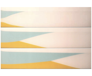
Sequence of photographs of two of our experiments, showing the deformation of a viscous current of diluted golden syrup (orange) loaded from above by a viscous current of glycerine (dyed blue). The upper current (glycerine) spills over an inviscid potassium carbonate solution and detaches from the lower current (diluted golden syrup) at the grounding line, where the lower current unloads and accumulates into a wedge. Panels (a–c) display experiment  $B$ shown 100 s before and 200 and 600 s after loading. Panels (d–g) display experiment $E$ shown 5, 10, 15 and 20 min after loading. Theoretical predictions after loading are overlain in black. The presence of a pressure-driven radial flow near the experimental source deviates from the assumptions of unidirectional thin-film flow. This is seen most in panels (a–c), in contrast to panels (d–g). See the end of § 3.2 for a discussion of the effect of this source flow.

For the upper, viscous current, we used either glycerine or diluted corn syrup, depending on the experiment. Each of these fluids were dyed with blue food colouring. Glycerine, used for the upper layer in some of the experiments, was undiluted and reused between experiments. As the viscosity of glycerine is strongly dependent upon water content, contamination with potassium carbonate solution and prolonged exposure to humidity led to a range of dynamic viscosities,  $\unicode[STIX]{x1D707}\approx 7{-}13~\text{g}~\text{cm}^{-1}~\text{s}^{-1}$, and a fixed density, $\unicode[STIX]{x1D70C}\approx 1.26~\text{g}~\text{cm}^{-3}$. Corn syrup solution, also used for the upper layer for one of the experiments, was diluted with water to achieve the density $\unicode[STIX]{x1D70C}\approx 1.375~\text{g}~\text{cm}^{-3}$ and dynamic viscosity $\unicode[STIX]{x1D707}\approx 49.7$.
For the lower, less viscous current, we used various concentrations of diluted golden syrup or diluted glycerine, depending on the experiment. Golden syrup solution, used for the lower layer in some of the experiments, was diluted with potassium carbonate solution of various concentrations to achieve densities of  $\unicode[STIX]{x1D70C}_{l}\approx 1.36{-}1.50~\text{g}~\text{cm}^{-3}$ and dynamic viscosities $\unicode[STIX]{x1D707}_{l}\approx 1.5{-}13~\text{g}~\text{cm}^{-1}~\text{s}^{-1}$. Glycerine solution, also used for the lower layer in some of the experiments, was diluted with potassium carbonate solution to achieve the density of $\unicode[STIX]{x1D70C}_{l}\approx 1.30{-}1.31~\text{g}~\text{cm}^{-3}$ and dynamic viscosity $\unicode[STIX]{x1D707}_{l}\approx 0.8{-}1.85~\text{g}~\text{cm}^{-1}~\text{s}^{-1}$.
We measured the viscosities using U-tube viscometers, and the densities using hydrometers, before each experiment. A complete list of parameter values is provided in table 1. We prefilled the Hele-Shaw cell with salt (potassium carbonate) solution of density  $\unicode[STIX]{x1D70C}_{s}\approx 1.3{-}1.4~\text{g}~\text{cm}^{-3}$ up to a specified height $S\approx 5.5{-}20~\text{cm}$ before each experiment.
The two viscous fluids were supplied at measured constant fluxes by means of peristaltic pumps connected at one end of the Hele-Shaw cell. We maintained a constant depth of salt solution by manual adjustment of an outflow valve, counteracting the rise in depth caused by its displacement by the two viscous fluids. For each experiment, the density of the salt solution was taken such that  $\unicode[STIX]{x1D70C}<\unicode[STIX]{x1D70C}_{s}<\unicode[STIX]{x1D70C}_{l}$, so that the less viscous fluid flowed over the salt solution, and the more viscous fluid intruded beneath the salt solution. Initially, the upper layer floated entirely over the inviscid layer and the lower layer intruded entirely beneath the inviscid layer, as shown in figure 2(a). Subsequently, after the two viscous currents exceeded a threshold thickness near the source, they made contact with each other, as shown in the sequence of photographs in figure 2(b,c). The two viscous fluids detached from one another at a locus referred to as the grounding line. The lower layer was observed to accumulate in a wedge-shaped region near the grounding line. A supplementary movie of one of our experiments is available at https://doi.org/10.1017/jfm.2020.393.
We measured the wedge angles from recorded images. Issues with photographic resolution and some dissolution between the corn syrup, glycerine solution and potassium carbonate solution led to sources of measurement error. Results of these experiments are presented below in comparison with theoretical predictions, which we describe next.
Parameter values used in our experiments.

Schematic diagram illustrating the side profile (a) and plan view (b) of the flow of two superposed thin films of fluid spreading into an inviscid ocean. The grounding line is the trijunction between the three fluids.

3 Theoretical development
To construct a theoretical model for our experiments, we consider a viscous fluid of density  $\unicode[STIX]{x1D70C}$ and dynamic viscosity $\unicode[STIX]{x1D707}$ spreading under its own weight over another viscous fluid of higher density $\unicode[STIX]{x1D70C}_{l}$ and dynamic viscosity $\unicode[STIX]{x1D707}_{l}$, which spreads under its own weight and the weight of the fluid above it over a rigid base $z=b(x)$ as shown in figure 3. The fluids are confined to a vertical Hele-Shaw cell of width $w$ and intrude into an inviscid layer of fluid of constant depth $S$ and density $\unicode[STIX]{x1D70C}_{s}$ such that $\unicode[STIX]{x1D70C}<\unicode[STIX]{x1D70C}_{s}<\unicode[STIX]{x1D70C}_{l}$. We assume the density of the inviscid layer is fixed. There are two regions: a loaded region $0\leqslant x\leqslant x_{G}(t)$, in which the two viscous fluids make contact with one another; and an unloaded region $x\geqslant x_{G}(t)$, in which the upper viscous current floats entirely over the inviscid layer and the lower viscous current intrudes entirely beneath it. We denote the upper surface height of the upper and lower viscous currents by $H(x,t)$ and $h(x,t)$, respectively. We assume that the upper surface of the inviscid layer remains fixed at the point $x=x_{N}$, where the ice–water interface (the calving front) intersects the upper, free surface of the inviscid layer. We also note that the momentum balance within the inviscid layer translates to a hydrostatic pressure balance, which directly affects the rate of the gravitational spreading of the unloaded till.
We consider viscous and buoyancy forces and assume that inertia and the effects of mixing and surface tension at the interface between the layers are negligible. We assume that lateral viscous shear stresses provide the leading-order resistance to the flow (Huppert Reference Huppert1986; Pegler et al. Reference Pegler, Kowal, Hasenclever and Worster2013) of both viscous currents. Formally, we consider  $w\ll H\ll L$, where $L$ is any of the horizontal extents of the sheet, the shelf and the till, and apply the approximations of lubrication theory. This is an idealised limit relevant to our experiments.
Under the thin-film approximation the volumetric flux of the lower fluid (till) in the loaded region can be found to be
 $$\begin{eqnarray}q_{l}=-\frac{\unicode[STIX]{x1D70C}gw^{2}}{12\unicode[STIX]{x1D707}_{l}}(h-b)\left(\frac{\unicode[STIX]{x1D70C}_{l}-\unicode[STIX]{x1D70C}}{\unicode[STIX]{x1D70C}}\frac{\unicode[STIX]{x2202}h}{\unicode[STIX]{x2202}x}+\frac{\unicode[STIX]{x2202}H}{\unicode[STIX]{x2202}x}\right),\quad 0\leqslant z\leqslant h,\end{eqnarray}$$
(Woods & Mason Reference Woods and Mason2000). The lower current is driven by its own weight as well as the weight of the fluid above it.
In the unloaded region, the lower current propagates independently of the upper current – that is, the shelf. This is because the weight of the shelf, which is assumed to obey Archimedes’ law of floatation, is equal to the weight of the water column that it has displaced. This implies that the value of the pressure, and hence the horizontal pressure gradient, at any given distance  $z$ above the $x$-axis, is indifferent to whether or not an ice shelf is overlying it. The pressure at $z=h$ is thus given hydrostatically by
 $$\begin{eqnarray}p_{l}|_{z=h}=\unicode[STIX]{x1D70C}_{s}g(s-h)\end{eqnarray}$$
throughout the unloaded region, giving rise to the hydrostatic pressure
 $$\begin{eqnarray}p_{l}=\unicode[STIX]{x1D70C}_{l}g(h-z)+\unicode[STIX]{x1D70C}_{s}g(s-h)\end{eqnarray}$$
within the unloaded layer of underlying fluid. The corresponding horizontal pressure gradient,
 $$\begin{eqnarray}\frac{\unicode[STIX]{x2202}p_{l}}{\unicode[STIX]{x2202}x}=(\unicode[STIX]{x1D70C}_{l}-\unicode[STIX]{x1D70C}_{s})g\frac{\unicode[STIX]{x2202}h}{\unicode[STIX]{x2202}x},\end{eqnarray}$$
 thus depends upon the gradient in the lower-layer thickness scaled by the density difference between it and the overlying inviscid layer throughout the unloaded region, not just beyond the front of the shelf  $x_{N}$. A horizontal force balance thus gives
 $$\begin{eqnarray}\unicode[STIX]{x1D707}\frac{\unicode[STIX]{x2202}^{2}u}{\unicode[STIX]{x2202}y^{2}}=(\unicode[STIX]{x1D70C}_{l}-\unicode[STIX]{x1D70C}_{s})g\frac{\unicode[STIX]{x2202}h}{\unicode[STIX]{x2202}x},\end{eqnarray}$$
from which it is possible to obtain the velocity field within the underlying layer and an expression for the depth-integrated volume flux
 $$\begin{eqnarray}q_{l}=-\frac{\unicode[STIX]{x1D70C}_{l}-\unicode[STIX]{x1D70C}_{s}}{\unicode[STIX]{x1D70C}_{l}}\frac{\unicode[STIX]{x1D70C}_{l}gw^{2}}{12\unicode[STIX]{x1D707}_{l}}(h-b)\frac{\unicode[STIX]{x2202}h}{\unicode[STIX]{x2202}x}\end{eqnarray}$$
(cf. Huppert Reference Huppert1986).
These fluxes are used within equations describing mass conservation to determine the full time-dependent evolution of the flows. We use the scalings
 $$\begin{eqnarray}(h,H,z)\equiv S({\hat{h}},{\hat{H}},z),\quad x\equiv {\mathcal{X}}\hat{x}\equiv \left(\frac{\unicode[STIX]{x1D70C}gw^{2}S^{2}}{12\unicode[STIX]{x1D707}q_{0}}\right)\hat{x},\end{eqnarray}$$
 $$\begin{eqnarray}t\equiv {\mathcal{T}}\hat{t}\equiv \left(\frac{\unicode[STIX]{x1D70C}gw^{2}S^{3}}{12\unicode[STIX]{x1D707}q_{0}^{2}}\right)\hat{t},\quad (q,q_{l})=q_{0}(\hat{q},\hat{q}_{l}),\end{eqnarray}$$
to non-dimensionalise the governing equations. The dimensionless parameters appearing throughout these equations are given by
 $$\begin{eqnarray}{\mathcal{M}}=\frac{\unicode[STIX]{x1D707}}{\unicode[STIX]{x1D707}_{l}},\quad {\mathcal{B}}=\frac{\unicode[STIX]{x1D6FC}{\mathcal{X}}}{S},\quad {\mathcal{Q}}=\frac{q_{l0}}{q_{0}},\quad {\mathcal{D}}_{l}=\frac{\unicode[STIX]{x1D70C}_{l}-\unicode[STIX]{x1D70C}}{\unicode[STIX]{x1D70C}},\quad {\mathcal{D}}_{s}=\frac{\unicode[STIX]{x1D70C}_{s}-\unicode[STIX]{x1D70C}}{\unicode[STIX]{x1D70C}_{s}}.\end{eqnarray}$$
 These describe the ratio of the viscosities of the two layers, the dimensionless bed slope in terms of the dimensional slope  $\unicode[STIX]{x1D6FC}$ for a sloped bed $b=\unicode[STIX]{x1D6FC}x$, the ratio of the source fluxes $q_{l0}$ and $q_{0}$ for the lower and upper layers, respectively, the dimensionless density difference between the upper and lower layers, and the dimensionless density difference between the upper layer and the inviscid ocean. For convenience, we also define the dimensionless density difference between the lower layer and the inviscid layer as
 $$\begin{eqnarray}{\mathcal{D}}_{ls}=\frac{\unicode[STIX]{x1D70C}_{l}-\unicode[STIX]{x1D70C}_{s}}{\unicode[STIX]{x1D70C}}={\mathcal{D}}_{l}-\frac{{\mathcal{D}}_{s}}{1-{\mathcal{D}}_{s}},\end{eqnarray}$$
which is useful in reducing the lower-layer flux in the unloaded region to
 $$\begin{eqnarray}q_{l}=-{\mathcal{M}}D_{ls}\frac{{\mathcal{X}}q_{0}}{S^{2}}(h-b)\frac{\unicode[STIX]{x2202}h}{\unicode[STIX]{x2202}x}.\end{eqnarray}$$
Under the non-dimensionalisation (3.7)–(3.8) and after dropping hats, the governing equations are summarised by
 $$\begin{eqnarray}q=-(H-h)\frac{\unicode[STIX]{x2202}H}{\unicode[STIX]{x2202}x},\quad q_{l}=-{\mathcal{M}}(h-{\mathcal{B}}x)\left({\mathcal{D}}_{l}\frac{\unicode[STIX]{x2202}h}{\unicode[STIX]{x2202}x}+\frac{\unicode[STIX]{x2202}H}{\unicode[STIX]{x2202}x}\right)\quad (x\leqslant x_{G}),\end{eqnarray}$$
 $$\begin{eqnarray}q=-\frac{1}{{\mathcal{D}}_{s}}(H-1)\frac{\unicode[STIX]{x2202}H}{\unicode[STIX]{x2202}x},\quad q_{l}=-{\mathcal{M}}{\mathcal{D}}_{ls}(h-{\mathcal{B}}x)\frac{\unicode[STIX]{x2202}h}{\unicode[STIX]{x2202}x}\quad (x\geqslant x_{G}),\end{eqnarray}$$
 $$\begin{eqnarray}\frac{\unicode[STIX]{x2202}H}{\unicode[STIX]{x2202}t}=-\frac{\unicode[STIX]{x2202}q}{\unicode[STIX]{x2202}x}-\frac{\unicode[STIX]{x2202}q_{l}}{\unicode[STIX]{x2202}x}\quad (x\leqslant x_{G}),\quad \frac{\unicode[STIX]{x2202}H}{\unicode[STIX]{x2202}t}=-{\mathcal{D}}_{s}\frac{\unicode[STIX]{x2202}q}{\unicode[STIX]{x2202}x}\quad (x\geqslant x_{G}),\end{eqnarray}$$
 $$\begin{eqnarray}\frac{\unicode[STIX]{x2202}h}{\unicode[STIX]{x2202}t}=-\frac{\unicode[STIX]{x2202}q_{l}}{\unicode[STIX]{x2202}x}\quad (0\leqslant x\leqslant x_{B}),\end{eqnarray}$$
subject to the flux conditions
 $$\begin{eqnarray}q=1,\quad q_{l}={\mathcal{Q}}\quad (x=0),\quad q=0\quad (x=x_{N}),\quad q_{l}=0\quad (x=x_{B}),\end{eqnarray}$$
the floatation condition, namely that the grounding line is the position at which the ice first begins to float according to Archimedes flotation (see e.g. Robison, Huppert & Worster Reference Robison, Huppert and Worster2010; Pegler et al. Reference Pegler, Kowal, Hasenclever and Worster2013), and the continuity conditions
 $$\begin{eqnarray}H^{-}=H^{+}=\frac{1-{\mathcal{D}}_{s}h^{-}}{1-{\mathcal{D}}_{s}},\quad h,q,q_{l}\quad \text{continuous}\quad (x=x_{G}),\end{eqnarray}$$
 where the superscripts  $^{+}$ and $^{-}$ refer to quantities evaluated just to the right and just to the left of the grounding line, respectively. The first of these, namely continuity of thickness, originates from a longitudinal stress balance at the grounding line. Together with the continuity of flux, the stress balance reduces to a simple condition of continuity of thickness. This is the case for strongly confined ice sheets, which contrasts with naturally confined (Kowal, Pegler & Worster Reference Kowal, Pegler and Worster2016) or purely two-dimensional ice sheets (Robison et al. Reference Robison, Huppert and Worster2010). The remaining frontal positions evolve kinematically,
 $$\begin{eqnarray}{\dot{x}}_{N}=-\frac{\unicode[STIX]{x2202}H}{\unicode[STIX]{x2202}x},\quad (x=x_{N}),\quad {\dot{x}}_{B}=-{\mathcal{M}}{\mathcal{D}}_{ls}\frac{\unicode[STIX]{x2202}h}{\unicode[STIX]{x2202}x},\quad (x=x_{B}).\end{eqnarray}$$
These kinematic conditions have been obtained by relating the fluxes of the two layers to their thicknesses. We have dropped hats for convenience.
3.1 Local unloading condition
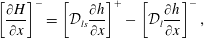
In what follows, we focus on the fluxes themselves to show how the mismatch between the loaded and unloaded regions results in the formation of a wedge in the grounding zone. In particular, wedge formation can be understood in terms of a local unloading condition
 $$\begin{eqnarray}\left[{\mathcal{D}}_{l}\frac{\unicode[STIX]{x2202}h}{\unicode[STIX]{x2202}x}+\frac{\unicode[STIX]{x2202}H}{\unicode[STIX]{x2202}x}\right]^{-}=\left[{\mathcal{D}}_{ls}\frac{\unicode[STIX]{x2202}h}{\unicode[STIX]{x2202}x}\right]^{+},\end{eqnarray}$$
 in terms of the density differences  ${\mathcal{D}}_{l}$ and ${\mathcal{D}}_{ls}$. We note that this condition is independent of bed slope. Equation (3.19) expresses the balance of fluxes of till either side of the grounding zone obtained from the continuity conditions (3.17) and the expressions (3.12b) and (3.13b) for the lower-layer fluxes in the loaded and unloaded regions. This balance directly translates to a balance of the horizontal pressure gradient across the grounding zone, as the fluxes of loaded and unloaded till are proportional to the pressure gradient within each region. This simplification holds as long as the loaded and unloaded parts of till are resisted dominantly by the same type of shear stress (in this case, transverse shear).
The unloading condition shows that a wedge will form, that is,  $(\unicode[STIX]{x2202}h/\unicode[STIX]{x2202}x)^{-}>0$, if
 $$\begin{eqnarray}(-\unicode[STIX]{x2202}H/\unicode[STIX]{x2202}x)^{-}>{\mathcal{D}}_{ls}(-\unicode[STIX]{x2202}h/\unicode[STIX]{x2202}x)^{+}.\end{eqnarray}$$
 The condition  $(\unicode[STIX]{x2202}h/\unicode[STIX]{x2202}x)^{-}>0$ is a geometrical description of the fact that fluid accumulates at the grounding zone. In other words, the inequality (3.20) implies that a wedge will form if the flux of till driven by the glaciostatic pressure gradient of the overlying ice is greater than the flux of till ahead of the grounding zone. This fundamental principle can be applied to more detailed models of grounding zones, for which different viscous couplings modify the balance (3.19) (see Kowal & Worster Reference Kowal and Worster2020).
3.2 Numerical and experiment results
Equations (3.12)–(3.18) form a free boundary problem involving both time and space, which we solved numerically by applying a second-order, finite-difference scheme to discretise the equations in space after mapping three parts of the domain to three fixed intervals, and integrating in time. Namely, (i) we mapped the loaded region  $[0,x_{G}]$ to the fixed interval $[0,1]$ in order to solve for the evolution of the ice sheet and loaded till on a fixed interval; (ii) we mapped the unloaded region $[x_{G},x_{B}]$ to the fixed interval $[0,1]$ in order to solve for the evolution of the unloaded till; and (iii) we mapped the region $[x_{G},x_{N}]$ corresponding to the ice shelf to the fixed interval $[0,1]$, in order to solve for the evolution of the ice shelf. These three maps introduce the three free boundary positions $x_{G},x_{B}$ and $x_{N}$ and their time derivatives into the governing system of partial differential equations. However, the advantage of this approach is that it is possible to discretise the transformed governing equations on a fixed domain. The transformed system of equations is given explicitly in appendix A in each of the domains. In order to proceed with the computations, it is necessary to specify the evolution of the three free boundary positions, which we did by applying the kinematic conditions (3.18) to evolve $x_{B}$ and $x_{N}$ and a variant of the constraint (3.17a), describing Archimedean floatation, to evolve $x_{G}$.
The remaining boundary and jump conditions were used to constrain the left- and right-hand endpoints of the discretised set of equations in each of the subregions. The system was evolved from an initial condition consisting of a similarity solution describing the ice shelf fed at constant flux at the source, a similarity solution describing the unloaded till, and a thin, trapezoidal ice sheet and loaded till of width  $\unicode[STIX]{x0394}x=10^{-3}$ so that $x_{G}=10^{-3}$ at $t=0$. Initial values for $x_{B}$ and $x_{N}$ were specified by the similarity solutions. We refer the reader to Pegler et al. (Reference Pegler, Kowal, Hasenclever and Worster2013) for a similar treatment and Huppert (Reference Huppert1986) for explicit forms for the similarity solutions used as initial conditions.
Solutions of the full system of partial differential equations for  ${\mathcal{Q}}=0.5$, ${\mathcal{D}}_{l}=0.08$, ${\mathcal{D}}_{ls}=0.02$ and (a) ${\mathcal{M}}=5$, (b) ${\mathcal{M}}=50$, (c) ${\mathcal{M}}=500$ at $t=100$ s. Each panel shows the thickness profiles of the two layers intruding into an inviscid ocean as functions of $x$. The underlying viscous fluid accumulates in a wedge-shaped region near the grounding zone. The loaded, underlying layer is thinner when its viscosity is lower.

The governing equations depend on four dimensionless parameters, namely  ${\mathcal{M}}$, ${\mathcal{D}}_{l}$, ${\mathcal{D}}_{ls}$ and $Q$ for currents propagating over a flat, horizontal base. A fifth dimensionless parameter ${\mathcal{B}}$ appears if the base is inclined at a small, non-zero angle to the horizontal. In the latter case, ${\mathcal{B}}$ characterises the dimensionless slope of the base. We integrated our model numerically to produce some illustrative results (figure 4) and to demonstrate the effect of the relative viscosity of ice and till. The values of the parameters ${\mathcal{Q}}$, ${\mathcal{D}}_{l}$ and ${\mathcal{D}}_{ls}$ used in these computations are commensurate with our experiments. The viscosity ratio ${\mathcal{M}}$ used in figure 4(a) is also commensurate with our experiments. In figures 4(b) and 4(c), we illustrate the effect of increasing viscosity ratio, showing in particular that the lubricating layer is thin at large viscosity ratios, which is typical of glaciological settings.
Comparison of our experimental data (symbols) for experiments A–I against the local condition (3.19) (solid line). All quantities are shown in unscaled variables. The data are shown only for times for which  $x_{G}>2{\mathcal{R}}$.

We have also overlain our theoretical predictions onto representative photographs of our experiments in figure 2. The disagreement between experiment and theory at early times comes from the presence of a pressure-driven radial flow near the experimental source, which deviates from the assumptions of unidirectional thin-film flow used in our theory. Such a pressure-driven, radial flow is seen to affect the flow most significantly in panels (a–c), in contrast to panels (d–g). Specifically, the flow is driven by a radial pressure gradient within a transition region  $r\sim {\mathcal{R}}\equiv 24\unicode[STIX]{x1D708}q_{0}/\unicode[STIX]{x03C0}{\mathcal{D}}_{s}gw^{2}$ near the source, which dominates the system at early times (Pegler et al. Reference Pegler, Kowal, Hasenclever and Worster2013).
Absolute error for our experimental data against the local condition (3.19) as a function of time. All the quantities are unscaled and dimensional in the centimetre–gram–second (known as CGS) system of units. The data reported in figure 5, for which  $x_{G}>2{\mathcal{R}}$, are shown using filled markers, and the remaining data, seen at early times owing to deviations near the experimental source, are shown using unfilled markers. As time progresses, the experimental data converge towards the prediction (3.19).

We test the local unloading condition (3.19) against our experimental data in figure 5. Specifically, rearranging this condition gives
 $$\begin{eqnarray}\left[\frac{\unicode[STIX]{x2202}H}{\unicode[STIX]{x2202}x}\right]^{-}=\left[{\mathcal{D}}_{ls}\frac{\unicode[STIX]{x2202}h}{\unicode[STIX]{x2202}x}\right]^{+}-\left[{\mathcal{D}}_{l}\frac{\unicode[STIX]{x2202}h}{\unicode[STIX]{x2202}x}\right]^{-},\end{eqnarray}$$
 which directly corresponds to the  $x$- and $y$-axes of figure 5. The closer the experimental data are to the line $y=x$, the better the condition is satisfied. All quantities are shown with respect to unscaled variables. In this experimental comparison, we consider only the data for which $x_{G}>2{\mathcal{R}}$, so that the region near the grounding line is less affected by the source flow. Figure 5 shows good agreement between theory and experiment over a wide range of experimental parameters, giving us confidence in the physical principles incorporated in our modelling.
As mentioned previously, the experiments conform more closely with the thin-film theory as time progresses. This is shown in figure 6, where we show the absolute value of the difference between the two sides of (3.21) as a function of time in dimensional units (seconds). We have plotted all of our data in this figure and indicate which data were most influenced by the initial pressure-driven flow ( $x_{G}<2{\mathcal{R}}$), which was excluded from figure 5.
In natural settings, the effective viscosity of till at various locations on Earth varies from  $7.5\times 10^{6}{-}4\times 10^{12}$ Pa s, with the lower reading taken from beneath Bindschadler Ice Stream in a fit to a model of tidal response, and the upper reading taken from strain rate data from Bakaninbreen, Svalbard (Boulton & Hindmarsh Reference Boulton and Hindmarsh1987; Blake, Clarke & Gerin Reference Blake, Clarke and Gerin1992; Humphrey et al. Reference Humphrey, Kamb, Fahnestock and Engelhardt1993; Fischer & Clarke Reference Fischer and Clarke1994; Porter & Murray Reference Porter and Murray2001; Anandakrishnan et al. Reference Anandakrishnan, Voigt, Alley and King2003; Cuffey & Paterson Reference Cuffey and Paterson2010). For comparison, the effective viscosity of glacial ice ranges from $5\times 10^{12}{-}10^{15}$ Pa s, depending on the temperature and other variables (Cuffey & Paterson Reference Cuffey and Paterson2010), giving rise to viscosity ratios that are much greater than those achieved in our experiments. Such natural viscosity ratios lead to much thinner underlying layers, which unlike those observed in figure 4, would seem indistinguishable from the horizontal axis, to the eye. Till densities, $\unicode[STIX]{x1D70C}_{l}$, at 10 %–30 % water content and a particle density of $2.65~\text{Mg}~\text{m}^{-3}$ vary between $1.92$ and $2.30~\text{Mg}~\text{m}^{-3}$ (Clarke Reference Clarke2017, Reference Clarke2018), which, together with a typical ocean density of $\unicode[STIX]{x1D70C}_{s}\approx 1~\text{g}~\text{cm}^{-3}$ and ice density of $0.92~\text{g}~\text{cm}^{-3}$, gives rise to dimensionless density differences ${\mathcal{D}}_{l}\approx 1.1{-}1.5$, ${\mathcal{D}}_{s}\approx 0.08$ and ${\mathcal{D}}_{ls}\approx 1{-}1.4$. These higher density differences again lead to thinner underlying layers than those observed in figure 4.
4 Discussion and conclusions
We conducted an experimental and theoretical study of the formation of sedimentary wedges, or till deltas, at the grounding zones of ice streams, and we presented a fluid-mechanical explanation of the formation of these wedges. We explained the formation of these wedges in terms of the hydrostatic loading and unloading of the underlying till at the grounding zone. The difference in loading and unloading leads to a decreasing flux of till beneath the ice as the grounding zone is approached, resulting in the formation of a grounding zone wedge.
We demonstrated this fundamental mechanism by developing a theoretical thin-film model, which we compared against our analogue laboratory experiments that we conducted in a confined setting. The formation mechanism is most clearly seen when horizontal shear stresses dominate the flow, as is the case in strongly confined settings. We found that a similar wedge of underlying fluid forms spontaneously at the grounding line of our experiments and have quantified wedge formation in terms of a local unloading condition relating wedge slopes either side of the grounding line, based on a balance of fluxes of till across the grounding line. There is good agreement with our experiments.
The down-flow wedge slopes in these calculations are generally gentler than those of grounding zone wedges found in nature. We anticipate that incorporating the non-Newtonian, shear-thinning rheology of till would generate steeper down-flow wedge slopes.
These fundamental ideas, explained here using Newtonian rheology and a simple geometry, can be extended to more geophysically relevant settings and rheologies typical of natural marine ice sheets by considering unconfined, two-dimensional geometries, in which wedge formation is modified by different viscous couplings between ice and till (Kowal & Worster Reference Kowal and Worster2020).
Acknowledgements
We are grateful to Dr M. Hallworth for his valuable help with our experiments and the technicians of the G.K. Batchelor Laboratory for assistance with the set-up of our experiments. K.N.K. was supported by an NERC doctoral training grant.
Declaration of interests
The authors report no conflict of interest.
Supplementary movie
Supplementary movie is available at https://doi.org/10.1017/jfm.2020.393.
Appendix A
The governing equations are solved numerically by mapping the domain to fixed intervals and discretising in the transformed variables. The transformations and resulting transformed equations are listed below, in each domain.
A.1 Loaded region
In the loaded region  $x<x_{G}$, we define the transformation $\unicode[STIX]{x1D709}=x/x_{G}$, $\unicode[STIX]{x1D70F}=t$, under which the flux of each of the two layers becomes
 $$\begin{eqnarray}\displaystyle & \displaystyle q=-\frac{1}{x_{G}}(H-h)\frac{\unicode[STIX]{x2202}H}{\unicode[STIX]{x2202}\unicode[STIX]{x1D709}}, & \displaystyle\end{eqnarray}$$
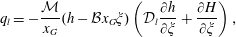 $$\begin{eqnarray}\displaystyle & \displaystyle q_{l}=-\frac{{\mathcal{M}}}{x_{G}}(h-{\mathcal{B}}x_{G}\unicode[STIX]{x1D709})\left({\mathcal{D}}_{l}\frac{\unicode[STIX]{x2202}h}{\unicode[STIX]{x2202}\unicode[STIX]{x1D709}}+\frac{\unicode[STIX]{x2202}H}{\unicode[STIX]{x2202}\unicode[STIX]{x1D709}}\right), & \displaystyle\end{eqnarray}$$
and the local mass conservation equations become
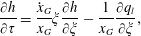 $$\begin{eqnarray}\displaystyle & \displaystyle \frac{\unicode[STIX]{x2202}h}{\unicode[STIX]{x2202}\unicode[STIX]{x1D70F}}=\frac{{\dot{x}}_{G}}{x_{G}}\unicode[STIX]{x1D709}\frac{\unicode[STIX]{x2202}h}{\unicode[STIX]{x2202}\unicode[STIX]{x1D709}}-\frac{1}{x_{G}}\frac{\unicode[STIX]{x2202}q_{l}}{\unicode[STIX]{x2202}\unicode[STIX]{x1D709}}, & \displaystyle\end{eqnarray}$$
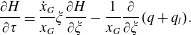 $$\begin{eqnarray}\displaystyle & \displaystyle \frac{\unicode[STIX]{x2202}H}{\unicode[STIX]{x2202}\unicode[STIX]{x1D70F}}=\frac{{\dot{x}}_{G}}{x_{G}}\unicode[STIX]{x1D709}\frac{\unicode[STIX]{x2202}H}{\unicode[STIX]{x2202}\unicode[STIX]{x1D709}}-\frac{1}{x_{G}}\frac{\unicode[STIX]{x2202}}{\unicode[STIX]{x2202}\unicode[STIX]{x1D709}}(q+q_{l}). & \displaystyle\end{eqnarray}$$
A.2 Unloaded till
In the unloaded region  $x_{G}<x<x_{B}$, we define the transformation $\unicode[STIX]{x1D701}=(x-x_{G})/(x_{B}-x_{G})$, $\unicode[STIX]{x1D70F}=t$, under which the flux of the underlying layer becomes
 $$\begin{eqnarray}q_{l}=-{\mathcal{M}}{\mathcal{D}}_{ls}\left[h-{\mathcal{B}}(x_{G}+(x_{B}-x_{G})\unicode[STIX]{x1D701})\right]\frac{1}{x_{B}-x_{G}}\frac{\unicode[STIX]{x2202}h}{\unicode[STIX]{x2202}\unicode[STIX]{x1D701}}\end{eqnarray}$$
and the corresponding mass conservation equation becomes
 $$\begin{eqnarray}\frac{\unicode[STIX]{x2202}h}{\unicode[STIX]{x2202}\unicode[STIX]{x1D70F}}=\frac{1}{x_{B}-x_{G}}\left({\dot{x}}_{G}+({\dot{x}}_{B}-{\dot{x}}_{G})\unicode[STIX]{x1D701}\right)\frac{\unicode[STIX]{x2202}h}{\unicode[STIX]{x2202}\unicode[STIX]{x1D701}}-\frac{1}{x_{B}-x_{G}}\frac{\unicode[STIX]{x2202}q_{l}}{\unicode[STIX]{x2202}\unicode[STIX]{x1D701}}.\end{eqnarray}$$
A.3 Shelf
Within the shelf  $x_{G}<x<x_{N}$, we define the transformation $\unicode[STIX]{x1D702}=(x-x_{G})/(x_{N}-x_{G})$, $\unicode[STIX]{x1D70F}=t$, under which the upper-layer flux within the shelf becomes
 $$\begin{eqnarray}q=-\frac{H-1}{{\mathcal{D}}_{s}(x_{N}-x_{G})}\frac{\unicode[STIX]{x2202}H}{\unicode[STIX]{x2202}\unicode[STIX]{x1D702}},\end{eqnarray}$$
and the corresponding mass conservation equation becomes
 $$\begin{eqnarray}\frac{\unicode[STIX]{x2202}H}{\unicode[STIX]{x2202}\unicode[STIX]{x1D70F}}=\frac{1}{x_{N}-x_{G}}({\dot{x}}_{G}+({\dot{x}}_{N}-{\dot{x}}_{G})\unicode[STIX]{x1D702})\frac{\unicode[STIX]{x2202}H}{\unicode[STIX]{x2202}\unicode[STIX]{x1D702}}-\frac{{\mathcal{D}}_{s}}{x_{N}-x_{G}}\frac{\unicode[STIX]{x2202}q}{\unicode[STIX]{x2202}\unicode[STIX]{x1D702}}.\end{eqnarray}$$


 Open access