





1. Introduction
Buoyant plumes in porous media may result from thermally driven convection or during injection scenarios involving fluids of different densities. Such flows are relevant within the context of numerous environmental and geophysical applications, such as groundwater contaminant transport due to waste leakage (MacFarlane et al. Reference MacFarlane, Cherry, Gillham and Sudicky1983), geothermal power production (Woods Reference Woods1999) and the geological storage of CO $_2$ emissions in subsurface reservoirs (Huppert & Neufeld Reference Huppert and Neufeld2014). Whilst such plumes have been studied in some detail far away from their origin, few studies have investigated the near-source behaviour. In particular, it is not known how the shape of a porous plume evolves close to the point of its formation, or whether this shape remains in a stable state or breaks apart due to instabilities. However, it is important to understand the characteristics of the near-field plume due to the effects that it can have on the pressure near the injection point and consequent flow rates (Gilmore et al. Reference Gilmore, Sahu, Benham, Neufeld and Bickle2022).
A wide body of literature has been developed surveying different buoyant flows in porous media. These include studies of convective instabilities in a Rayleigh–Bénard cell (Graham & Steen Reference Graham and Steen1994), convective shutdown behaviour (Hewitt, Neufeld & Lister Reference Hewitt, Neufeld and Lister2013a), the onset and evolution of convective fingers (Wooding, Tyler & White Reference Wooding, Tyler and White1997a; Wooding et al. Reference Wooding, Tyler, White and Anderson1997b), and mixing effects during injection into a porous medium (Lyu & Woods Reference Lyu and Woods2016). It has been demonstrated that a quasi-steady regime exists in both two- and three-dimensional Rayleigh–Bénard cells in which convection occurs in columnar structures (Hewitt, Neufeld & Lister Reference Hewitt, Neufeld and Lister2013b; Hewitt & Lister Reference Hewitt and Lister2017). For buoyant flows that are not thermally driven, but are instead driven by injection, similar columnar structures have been observed. For example, Gilmore et al. (Reference Gilmore, Sahu, Benham, Neufeld and Bickle2022) described the behaviour of a two-dimensional buoyant column of fluid with weakly varying thickness, resulting from leakage through an impermeable baffle. In that study, it was shown that the shape of the column affects the near-baffle pressure and consequent leakage rates, indicating the need to model such scenarios accurately. However, there is no study that describes the generic shape of a porous plume near its source, or the criteria for which this remains stable.
This study describes such a porous plume supplied by a constant injection (i.e. not thermally driven), focusing on its shape and stability in the near field (within a few plume-width scales) of its origin. We ignore the effects of mixing with the ambient fluid, since these occur over much greater length scales and are described by other studies (Sahu & Flynn Reference Sahu and Flynn2015; Lyu & Woods Reference Lyu and Woods2016). We establish the criteria for the existence of a steady-state regime, and we demarcate the parameter values for which this becomes unstable. In particular, if the injected fluid is supplied with a velocity much smaller than the buoyancy velocity (i.e. the equilibrium rise speed within the porous medium), then the interface separating the plume from the ambient fluid becomes unstable at a critical distance downstream. On the other hand, if the inlet velocity is sufficiently close to the buoyancy velocity, then this instability is suppressed and the plume maintains a steady shape.
We study both two-dimensional plumes resulting from a line source, and axisymmetric plumes resulting from a circular source, using input velocities that are significantly different from the buoyancy velocity (i.e. resulting in large variations in the plume width). This is in contrast to the study of Gilmore et al. (Reference Gilmore, Sahu, Benham, Neufeld and Bickle2022), which considered only weakly varying plume shapes in the two-dimensional case. In addition, we extend the analysis to unsteady flows and assess the stability of the plume shape in several different cases, whereas Gilmore et al. studied only the steady case.
The structure of the paper is as follows. In § 2, the flow scenario is described for both two-dimensional and axisymmetric plumes, deriving both analytical and numerical solutions in the steady state. Comparisons are also made with the porous media tank experiments of Gilmore et al. (Reference Gilmore, Sahu, Benham, Neufeld and Bickle2022). Section 3 treats the stability of these steady plume shapes using a linear perturbation analysis. Finally, § 4 closes with a discussion on the possible application of our results to injection scenarios during CO $_{2}$ sequestration, as well as other further extensions of this work.
2. Porous plumes in the near field of injection
We consider the constant injection  $Q$ of a fluid of density $\rho _1$ into an infinite porous medium saturated with a heavier fluid of density $\rho _2>\rho _1$, as illustrated in figure 1. (Note that this study also applies to the configuration of a heavier fluid injected into a lighter fluid, $\rho _2<\rho _1$, due to the Boussinesq approximation (Soltanian et al. Reference Soltanian, Amooie, Dai, Cole and Moortgat2016; Amooie, Soltanian & Moortgat Reference Amooie, Soltanian and Moortgat2018), in which case figure 1 is inverted.) For simplicity, we assume that the fluids have the same viscosity $\mu _1=\mu _2=\mu$, although this assumption is discussed in more detail later. Since the injected fluid is lighter than the ambient fluid, it rises upwards, forming an ascending plume of cross-sectional area $A(z,t)$.
Schematic diagram of the flow scenario in the case of a circular source. The injected fluid  $z\geq 0$ is fed by a flow $w_0$ through a disk region of area $A_0$, and speeds up to match the natural buoyancy velocity $w_b$ downstream. Hence the plume cross-section $A(z,t)$ thins out from $A_0$ to $A_\infty$ to conserve mass.
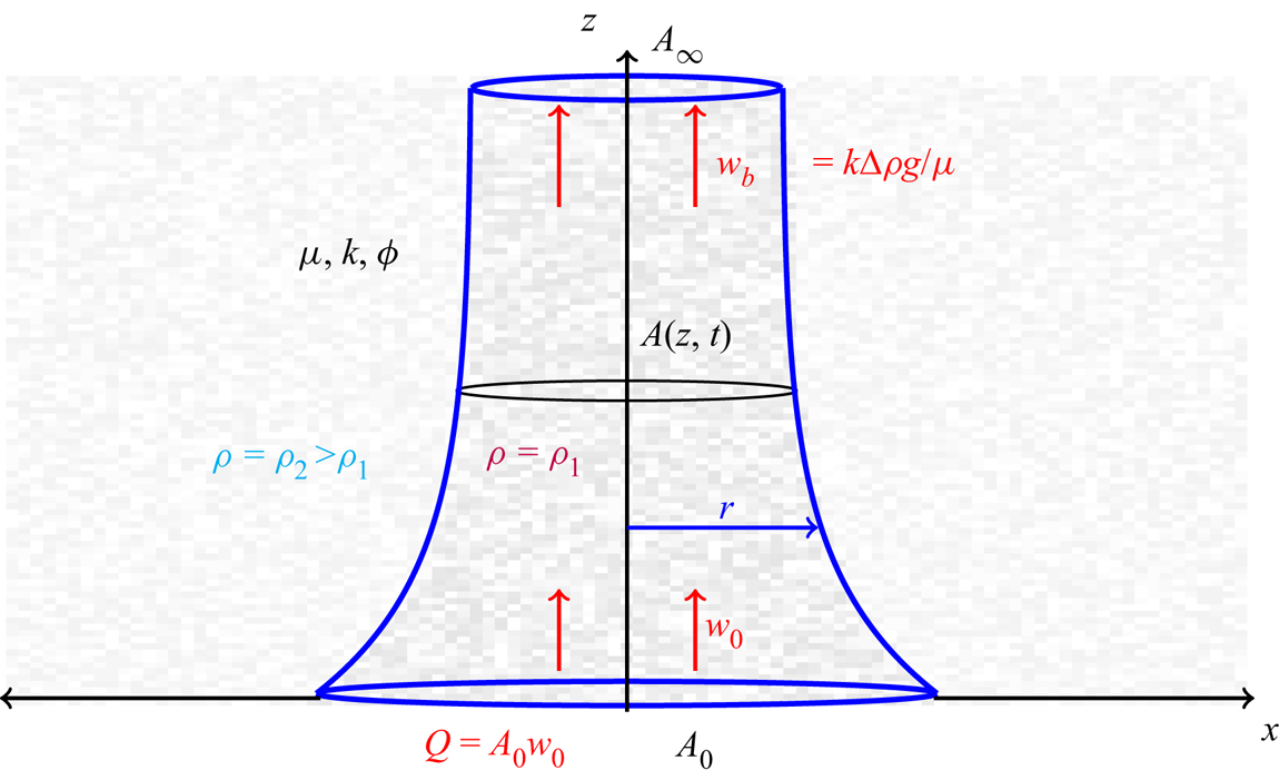
There are two spatial regimes characterised by  $A_0=A(0,t)$, the area at the point of injection. In the near-field regime $z={O}(A_0^{1/2})$, which is the focus of the current study, the plume adjusts its shape to conserve mass whilst matching the equilibrium buoyancy velocity of the porous medium (i.e. buoyancy balancing viscous resistance), and the effects of mixing with the ambient fluid are negligible. Over much greater length scales $z\gg A_0^{1/2}$, the injected fluid mixes with the ambient fluid, causing the buoyancy to decrease and the width of the plume to increase as the flow moves upwards. For example, the experiments of Sahu & Flynn (Reference Sahu and Flynn2015) revealed that plume-width changes due to dispersive mixing occur over vertical length scales $z= {O}(10 A_0^{1/2})$.
Therefore, in the current study, we neglect the effects of mixing and focus only on the changes in the plume shape due to mass conservation as it adjusts its velocity. Hence we treat the injected and ambient fluids as immiscible, such that the interface between them remains sharp (e.g. see sharp interface models of other gravity-driven flows; Huppert & Woods Reference Huppert and Woods1995). We consider both the case of injection from a line source, in which the resultant flow varies only in the horizontal ( $x$) and vertical ( $z$) directions, and injection from a circular source, in which the resultant flow is axisymmetric and varies with cylindrical coordinates ( $r$ and $z$), as shown in figure 1.
If the injection flow rate  $Q$ is sufficiently small, then we expect an instability to occur in which the shape of the plume $A(z,t)$ becomes unsteady due to the density contrast of a heavier fluid sitting above a lighter fluid (Rayleigh Reference Rayleigh1900; Taylor Reference Taylor1950). Likewise, we expect another regime corresponding to larger flow rates in which the shape remains steady, $A=A(z)$. The aim of this study is first to describe the steady-state regime for the near-field plume, and then to address the criteria for the stability of this steady state.
2.1. Steady plumes
To address the steady-state regime, we describe the shape of the plume  $A(z)$ above the injection height ( $z\geq 0$) in general terms that apply to both linear and circular sources. At the injection point, the vertical inflow velocity is
 \begin{equation} w_0=\frac{Q}{A_0}.\end{equation}
Likewise, the buoyancy velocity of the injected fluid, which is the equilibrium rise speed in the porous medium (i.e. buoyancy balancing viscous resistance), is given by
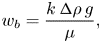 \begin{equation} w_b=\frac{k\,{\rm \Delta}\rho\,g}{\mu},\end{equation}
where  $k$ is the permeability of the medium, and ${\rm \Delta} \rho =\rho _2-\rho _1$. Due to mass conservation, the far field cross-section is given by $A_\infty =Q/w_b$. (Note that we use the term ‘far field’ here and throughout the paper to refer to the length scale over which the plume velocity approximately matches the buoyancy velocity. This is not to be confused with the even greater length scales over which the effects of mixing are important, since these are not studied here.) Hence the key dimensionless parameter in this study is the ratio between the inlet and buoyancy velocities,
 \begin{equation} W=\frac{w_0}{w_b}. \end{equation}
As the flow moves downstream (i.e. upwards), the plume must become thinner ( $A_\infty < A_0$) for sub-buoyancy velocities $W<1$ and thicker ( $A_\infty >A_0$) for super-buoyancy velocities $W>1$.
The flow within the injected fluid is governed by the Darcy equations
 \begin{gather} \boldsymbol{\nabla}\boldsymbol{\cdot}\boldsymbol{u}=0, \end{gather}
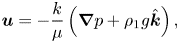 \begin{gather}\boldsymbol{u}={-}\frac{k}{\mu}\left( \boldsymbol{\nabla} p + \rho_1 g \hat{\boldsymbol{k}}\right), \end{gather}
where  $\boldsymbol {u}$ is the Darcy velocity vector, and $p$ is the pressure. The flow in the ambient fluid is coupled to the injected fluid only via the boundary conditions, which we discuss in the next subsection. Hence, for the purposes of this study, we omit further details of how to model the ambient flow outside the injected region, since the behaviour of the injected flow is of primary interest.
The Darcy equations (2.4)–(2.5) are accompanied by boundary conditions that take a different form depending on whether the flow is injected from a line source or a circular source. Hence we address the former and latter cases separately in §§ 2.2 and 2.4.
2.2. Plume shape: the case of a line source
In the case of the line source (with  $A(z)=a(z)\,d$, where $d$ is the depth in the third dimension), we impose boundary conditions within the injected fluid region of the form
 \begin{gather} u=0,\quad x=0, \end{gather}
 \begin{gather}w=w_0,\quad z=0, \end{gather}
 \begin{gather}w\rightarrow w_b,\quad z\rightarrow \infty, \end{gather}
 \begin{gather}u=w\,a'(z),\quad x=a(z), \end{gather}
 \begin{gather}p=p_a-\rho_2 g z,\quad x=a(z), \end{gather}
where  $p_a$ is the ambient hydrostatic pressure at $z=0$, and $a'(z)=\mathrm {d}a/\mathrm {d}z$. The above boundary conditions correspond with imposing symmetry on the $z$ axis (2.6), constant inflow at the source (2.7), matching with the far-field buoyancy velocity (2.8), and applying the kinematic (2.9) and dynamic conditions (2.10) at the sharp interface. For further details on the governing equations and boundary conditions for flow in porous media, see Bear (Reference Bear2013).
The above system (2.4)–(2.10) is a free boundary problem for both the flow and the shape of the interface  $a(z)$. To proceed, we seek a solution of the form
 \begin{gather} p=p_a-\rho_2 g z +\hat{p}, \end{gather}
 \begin{gather}u=\hat{u}, \end{gather}
 \begin{gather}w=w_b+\hat{w}, \end{gather}
where the hatted Darcy velocities satisfy
 \begin{gather} \hat{u}={-}(k/\mu) \hat{p}_x, \end{gather}
 \begin{gather}\hat{w}={-}(k/\mu) \hat{p}_z, \end{gather}
in which subscripts denote partial derivatives. Hence the hatted pressure satisfies the new system of equations
 \begin{gather} \nabla^2\hat{p}=0, \end{gather}
 \begin{gather}\hat{p}_x=0,\quad x=0 , \end{gather}
 \begin{gather}\hat{p}_z={\rm \Delta}\rho\,g(1-W),\quad z=0, \end{gather}
 \begin{gather}\hat{p}_z\rightarrow 0,\quad z\rightarrow \infty, \end{gather}
 \begin{gather}\hat{p}_x=(\hat{p}_z-{\rm \Delta} \rho\,g)\,a'(z),\quad x=a(z), \end{gather}
 \begin{gather}\hat{p}=0,\quad x=a(z). \end{gather}
The governing equation (2.16) is obtained by inserting (2.12)–(2.15) into the continuity equation (2.4), whereas (2.17)–(2.21) are obtained from each of the boundary conditions (2.6)–(2.10), respectively.
In the case where the inlet velocity is close to the buoyancy velocity ( $W\approx 1$), the solution to (2.16)–(2.21) was calculated by Gilmore et al. (Reference Gilmore, Sahu, Benham, Neufeld and Bickle2022) using the method of separation of variables, in which case
 \begin{equation}
\hat{p}\approx{-}(1-W){\frac{8\,{\rm \Delta} \rho\,g
a_0}{{\rm \pi}^2}}\sum_{n=0}^\infty
{\frac{({-}1)^n}{(2n+1)^2}}
\cos\left[{(}2n+1{)}{{\rm \pi}
{x}}/{2a_0}\right]\exp\bigl(-(2n+1){{\rm \pi}
z}/{2a_0}\bigr),\end{equation}
\begin{equation}
\hat{p}\approx{-}(1-W){\frac{8\,{\rm \Delta} \rho\,g
a_0}{{\rm \pi}^2}}\sum_{n=0}^\infty
{\frac{({-}1)^n}{(2n+1)^2}}
\cos\left[{(}2n+1{)}{{\rm \pi}
{x}}/{2a_0}\right]\exp\bigl(-(2n+1){{\rm \pi}
z}/{2a_0}\bigr),\end{equation}
where  $a_0=a(0)$. Likewise, the approximate plume shape is given by the solution to
 \begin{equation} a'(z)\approx{-}(1-W)\,\frac{4}{\rm \pi}\tanh^{{-}1}\left[\exp(-{\rm \pi} z/2 a_0)\right].\end{equation}
This is obtained from the linearised version of (2.20) (i.e.  $\hat {p}_x=-{\rm \Delta} \rho \,g\,a'(z)$ at $x=a_0$) after inserting the formula for the pressure (2.22). Then the infinite sum converges to the inverse hyperbolic tangent function in (2.23).
In the case where the inlet velocity and the buoyancy velocity are not similar ( $W\not \approx 1$), a numerical method must be used to calculate the solution. By converting to a set of scaled dimensionless variables
 \begin{equation} X=x/a(z),\quad Z=z/a_0,\quad P(X,Z)=\hat{p}(x,z)/{\rm \Delta} \rho\,g a_0,\quad \alpha(Z)= a(z)/a_0,\end{equation}
Laplace's equation (2.16) becomes
 \begin{equation} \left[\alpha^{{-}2}\,\partial_{XX}+\left(\partial_Z-X\alpha'\alpha^{{-}1}\,\partial_X\right)^2\right]P=0,\end{equation}
whilst the remaining boundary conditions become
 \begin{gather} P_X=0,\quad X=0, \end{gather}
 \begin{gather}P_Z-X\alpha'\alpha^{{-}1} P_X=1-W,\quad Z=0, \end{gather}
 \begin{gather}P_Z-X\alpha'\alpha^{{-}1} P_X\rightarrow 0,\quad Z\rightarrow \infty, \end{gather}
 \begin{gather}P_X={-}\alpha\alpha'- {\alpha'}^2P_X,\quad X=1, \end{gather}
 \begin{gather}P=0:\quad X=1. \end{gather}
The nonlinear system (2.25)–(2.30) is solved using Newton's method in combination with a finite difference scheme. The domain is discretised using a rectangular grid, with  $X\in [0,1]$ and $Z\in [0,H]$, where the boundary condition (2.28) is approximated at a large but finite value $H=10$. We calculate the solution for a variety of values of $W$ (the only dimensionless parameter of the problem), using an 8th-order finite difference scheme with a grid of $20\times 200$ points in the $X,Z$ directions (Note that in some cases – such as for $W>1$ – the discretisation was increased to $40\times 400$ points to resolve accurately sharp gradients in the plume shape near the origin.) By employing the method of continuation using incremental changes in $W$, Newton's method converges in approximately three steps (for each increment).
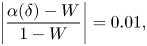
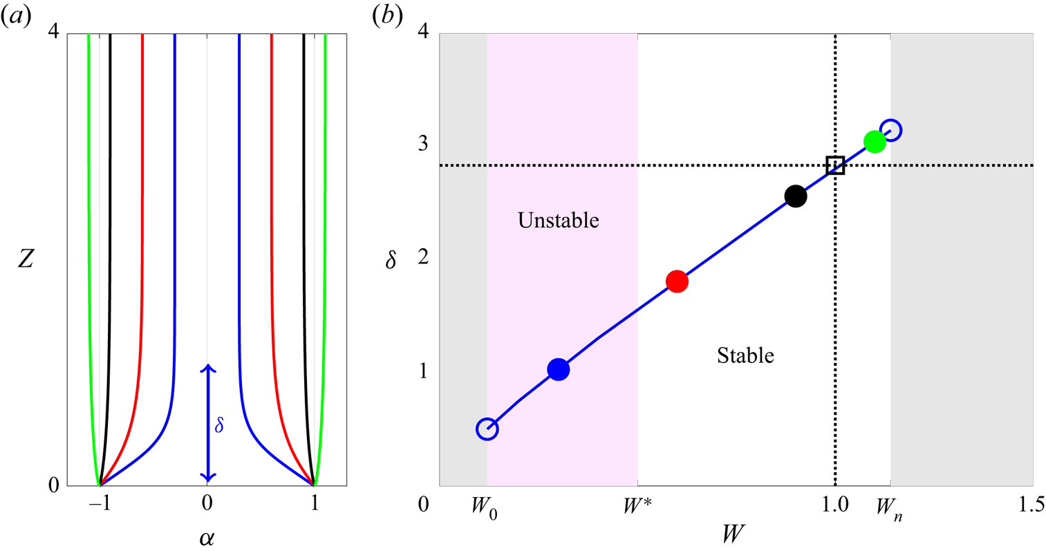
We plot examples of the shape  $\alpha (Z)$ in figure 2(a) for $W=0.3,0.6,0.9,1.1$. Thinning plumes are observed for $W<1$, whereas thickening plumes are observed for $W>1$, as expected. One salient feature of the analysis is the distance over which the plume approaches its far-field width $a_\infty$ (or $\alpha \rightarrow W$ in dimensionless terms). We define the $99\,\%$ boundary layer distance $\delta$ (dimensionless) as
 \begin{equation} \left|\frac{\alpha(\delta)-W}{1-W}\right|=0.01,\end{equation}
and this is plotted in figure 2(b) for different values of  $W$. We find that $\delta (W)$ is monotone increasing for $W\in [0.12,1.14]$. Outside this range, our numerical method fails to converge to a real-valued solution (which we discuss shortly), so no data are plotted. We also compare these values of $\delta$ with the analytical value in the case where $W$ is close to $1$ (e.g. via the solution to (2.23)). In this case, the boundary layer distance is independent of $W$ at leading order, and is given by the approximate value $\delta \approx 2.83$ (see dotted lines in figure 2b). We note that despite the fact that the boundary condition (2.28) is imposed at $Z\rightarrow \infty$, no more than a few plume-width scales are required for the plume to adjust to its far-field shape ( $99\,\%$ of the way, more specifically), as seen by the $\delta$ values in figure 2(b).
Numerical and analytical results for a thinning/thickening plume resulting from a line source. (a) Plume shape for different velocity ratios  $W=w_0/w_b$, and (b) $99\,\%$ boundary layer distance $\delta$ as defined in (2.31). Critical values $W_0$, $W^*$ and $W_n$ are related to the sign of the discriminant $\varDelta$ (see (2.32)) and the stability/existence of a steady solution. Dotted lines indicate the approximate solution when $W\approx 1$, for which the plume shape is given by the solution to (2.23).
Due to the kinematic boundary condition (2.29), for the solution to remain real-valued we require a non-negative discriminant
 \begin{equation} \Delta(Z):=\alpha^2-4\left.P_X\right|_{X=1}^2\geq 0,\end{equation}
for all values of  $Z$. By writing the pressure gradient as a dimensionless velocity $P_X=-U$, we see that (2.32) can be interpreted as a balance criterion between the width of the plume $\alpha$ and the horizontal velocity $U$ required to sustain that width. For example, a thinning plume ( $U<0$) with a shape that tapers to smaller than thickness $\alpha <-2U$ is not permitted by (2.32). In general, whenever (2.32) cannot be satisfied, this indicates that a smooth and continuous steady plume shape is not possible.
The behaviour of the discriminant function (2.32) depends on the value of the velocity ratio  $W$. There are four solution regimes defined by three values of the velocity ratio, $W^*\approx 0.5$, $W_n\approx 1.14$ and $W_0\approx 0.12$. For velocity ratios $W^*< W< W_n$, the discriminant is strictly positive, $\varDelta >0$, for all values of $Z$. For velocity ratios in the range $W_0< W< W^*$, the discriminant is non-negative, $\varDelta \geq 0$, but equals zero at some critical distance $Z=Z^*$ downstream of the inflow. For $0< W< W_0$ or $W>W_n$, Newton's method fails to converge to a real-valued solution, indicating that a steady solution in the form of a smooth continuous shape $\alpha (Z)$ may not exist. The four different solution regimes are illustrated with shading in figure 2(b). It should be noted that the sign of the discriminant is closely linked with the stability criteria for the plume, and we discuss this later, in § 3.
Before discussing the comparison with experiments, it is interesting to note the possible effects of the ambient fluid that we have so far neglected in this study. Within the ambient region, the flow satisfies a set of Darcy equations similar to (2.4)–(2.5) except with  $\rho =\rho _2$. Appropriate boundary conditions consist of the impermeability condition at the bottom boundary ( $w=0$ on $z=0$), far-field hydrostatic conditions ( $p \rightarrow p_a-\rho _2 g z$, as $x,z,\rightarrow \infty$), and the kinematic and dynamic boundary conditions, (2.9) and (2.10), at the interface $x=a(z)$. One can see immediately that a hydrostatic pressure profile $p=p_a-\rho _2 g z$ satisfies all of these conditions. Hence the flow in the ambient region is simply zero everywhere in the steady state, and therefore affects the injected fluid region only via the density difference.
It is also interesting to note that if we change the viscosity of the ambient fluid (i.e. such that  $\mu _2\neq \mu _1$), then this has no effect on the preceding argument. Therefore, it follows that the steady plume shape is independent of the viscosity ratio between the injected and ambient fluids, $M=\mu _1/\mu _2$. However, as we discuss later, in § 3, this is no longer true in the unsteady case.
2.3. Comparison with experiments
In this subsection, we compare our results for the steady plume shape (in the case of a line source) to the porous bead experiments of Gilmore et al. (Reference Gilmore, Sahu, Benham, Neufeld and Bickle2022). These experiments were conducted in a thin rectangular tank of dimensions  $40\times 70\,\mathrm {cm}^2$ in the $x,z$ directions and $1\,\mathrm {cm}$ thick in the transverse ( $y$) direction. The tank was filled with $3\,\mathrm {mm}$ Ballotini beads and initially saturated with fresh water. Salty water dyed with red food colouring was injected into the top of the tank, using different salt concentrations to modify the density contrast. Since salty water is heavier than fresh water, the experiments resulted in a falling plume rather than the rising plume studied at present. Therefore, we have inverted their experimental photos for comparison with our model. The inverted system behaves in approximately the same way as the current system due to the Boussinesq approximation (Soltanian et al. Reference Soltanian, Amooie, Dai, Cole and Moortgat2016; Amooie et al. Reference Amooie, Soltanian and Moortgat2018).
The focus of the Gilmore et al. (Reference Gilmore, Sahu, Benham, Neufeld and Bickle2022) study was on the leakage of salty water through a gap in an impermeable division midway down the tank. However, for comparison with the present study, we focus on the flow below this division only, and we ignore all the flow details above this. Therefore, we restrict our attention to the lower  $40\times 40\times 1\,\mathrm {cm}^3$ of their tank. In this way, the leakage rates of salty water into this lower section of the tank (which were calculated in their study) correspond to the injection flow rate $Q$ in our theoretical model. As described by Gilmore et al. (Reference Gilmore, Sahu, Benham, Neufeld and Bickle2022), both the leakage flux and the near-field plume shape within this lower section of the tank were approximately steady (after an initial transient). Hence, for comparison with our model, a constant inflow $Q$ and a steady shape $\alpha (Z)$ can be assumed to good approximation.
Examples of steady plumes from the study of Gilmore et al. (Reference Gilmore, Sahu, Benham, Neufeld and Bickle2022) are shown in experimental photographs in figures 3(a,b). The plume width at the inlet for each case is  $a_0=3,2.5$ cm, respectively. To calculate the velocity ratios $W$ for each case, we estimate the far-field plume width $a_\infty$ downstream, noting that $W=a_\infty /a_0$. This results in $W=0.58$ and $W=0.74$ for figures 3(a) and 3(b), respectively. We have also tried estimating $W$ using values of $w_0$ and $w_b=k\,{\rm \Delta} \rho \,g/\mu$ given by Gilmore et al. (i.e. using quoted values for the permeability, density, viscosity and leakage flux), which produces similar calculations.
Experimental photos (taken from the study of Gilmore et al. Reference Gilmore, Sahu, Benham, Neufeld and Bickle2022) of thinning plumes with (a)  $W=0.58$ and (b) $W=0.74$, compared with numerical (solid lines) and analytical (dotted lines) solutions for the steady plume shape in the case of a line source. The photos are partially obscured by a clamp (part of the apparatus), which is labelled for clarity.
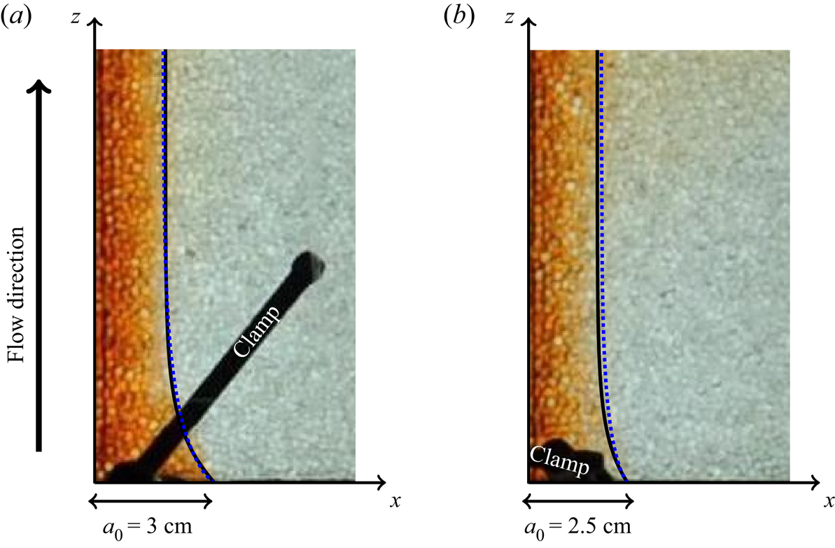
The steady plume shape predicted by our numerical model is compared to each of these photos with solid lines. The analytical approximation, given by integrating (2.23), is also shown with dotted lines. Overall, good agreement is observed between the numerical model, the analytical approximation and the experiments. Dispersion causes the plume shape to slightly diffuse downstream of the inlet, which is not captured by the sharp interface in our model.
One advantage of our simple model is that it depends on only a single dimensionless parameter  $W$, which is easily calculated by estimating the plume width at two locations (i.e. $a_0$ and $a_\infty$). A more complicated model that accounts for dispersion, for example, would require further parameter values of the fluid-medium properties, such as the diffusion and dispersion coefficients of the salt/dye.
2.4. Plume shape: the case of a circular source
In the case of a circular source, the boundary conditions (2.6)–(2.10) are replaced by corresponding conditions in cylindrical radial coordinates (e.g. with  $x$ replaced by $r$, and $u$ replaced by $u_r$, the radial velocity). In this case, the radius of the plume (measured from the $z$ axis) is given by $a(z)=(A(z)/{\rm \pi} )^{1/2}$. As before, we seek a solution of the form (2.11)–(2.13) (with $u$ replaced by $u_r$). The pressure $\hat {p}$ satisfies a system of equations similar to (2.16)–(2.21), with $x$ replaced by $r$. In the case where $W$ is close to unity, the solution is calculated by separation of variables (see Appendix A), giving
 \begin{equation} \hat{p}\approx{-}2(1-W)\,{\rm \Delta} \rho\,g a_0\sum_{n=1}^\infty \frac{J_0(j_{0,n}r/a_0)}{j_{0,n}^2\,J_1(j_{0,n})} \exp({-j_{0,n}z/a_0}),\end{equation}
where  $J_0$ and $J_1$ are the 0th- and 1st-order Bessel functions of the first kind, and $j_{0,n}$ is the $n$th zero of $J_0$. Likewise, the plume shape is given by the solution to
 \begin{equation} a'(z)\approx{-}2(1-W)\sum_{n=1}^\infty \frac{\exp({-j_{0,n}z/a_0})}{j_{0,n}}.\end{equation}
This is obtained from the linearised version of (2.20) in radial coordinates (i.e.  $\hat {p}_r=-{\rm \Delta} \rho \,g\,a'(z)$ at $r=a_0$) after inserting the formula for the pressure (2.33). By using the identity $J_0'(r)=-J_1(r)$, this simplifies to (2.34).
In the case where  $W$ is not close to unity, we calculate the solution via the numerical method described earlier. After introducing a scaled dimensionless radial coordinate
 \begin{equation} R=r/a(z),\end{equation}
Laplace's equation (2.16) becomes
 \begin{equation} \left[\alpha^{{-}2}R^{{-}1}\,\partial_{R}(R\,\partial_R)+\left(\partial_Z-R\alpha'\alpha^{{-}1}\, \partial_R\right)^2\right]P=0,\end{equation}
whilst the remaining boundary conditions stay the same as (2.26)–(2.30) except with  $X$ switched to $R$. The system of equations is solved using the same finite difference scheme as in § 2.2 (except with the radius truncated at a small but finite value $R=0.01$ to avoid a singular Laplacian). Likewise, a similar discriminant function is defined as
 \begin{equation} \Delta(Z):=\alpha^2-4\left.P_R\right|_{R=1}^2,\end{equation}
which indicates whether or not a real solution exists.
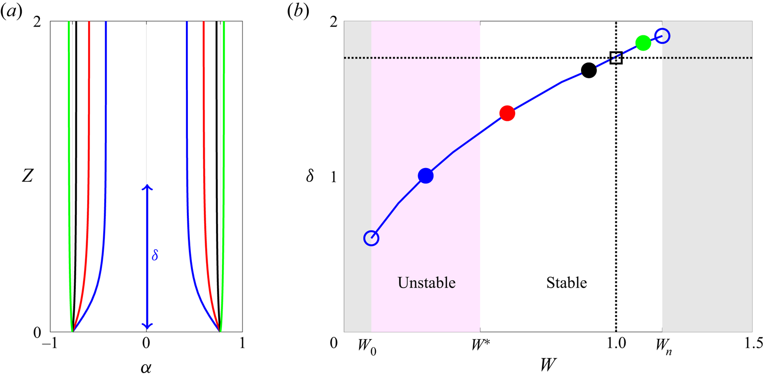
In figure 4(a), we display the steady plume shapes calculated for  $W=0.3,0.6,0.9,1.1$. Likewise, the $99\,\%$ boundary layer distance $\delta$ (as defined in (2.31)) is plotted in figure 4(b). Overall, the behaviour is similar to the case of a line source, except that the plume adjusts over a shorter vertical length scale, resulting in smaller values of $\delta$. The approximate solution calculated in the case where $W\approx 1$ (i.e. via integration of (2.34)) results in a boundary layer distance $\delta \approx 1.76$, as shown with dotted lines in figure 4(b). Critical values of the velocity ratio (see earlier discussion in § 2.2) are $W_0=0.1$, $W^*=0.5$ and $W_n=1.17$, which are very similar to the case of a line source.
Numerical and analytical results for a thinning/thickening axisymmetric plume resulting from a circular source. (a) Plume shape for different velocity ratios  $W$, and (b) $99\,\%$ boundary layer distance $\delta$ as defined in (2.31). Critical values $W_0$, $W^*$ and $W_n$ are related to the sign of the discriminant $\varDelta$ in (2.37) and the stability/existence of a steady solution. Dotted lines indicate the approximate solution when $W\approx 1$, for which the plume shape is given by the solution to (2.34).
3. Unsteady plumes and the criteria for stability
Unlike the previous sections, which have assumed a steady state, here we address the possibility of an unsteady flow by investigating the linear stability of the system. We divide the following analysis into several subsections that are distinguished by the velocity ratio  $W$. The first subsection addresses the case when $W_0< W< W^*$ such that the discriminant $\varDelta$ equals zero at a critical point downstream of the inlet. The second subsection addresses velocity ratios larger than this, $W^*< W< W_n$, for which the discriminant is always positive (see discussion at the end of § 2.2). In the former case, we demonstrate the existence of an infinitesimal perturbation to the steady plume shape that grows unbounded over time, and hence we show that such scenarios are inherently unstable. In the latter case, we show that such an instability cannot form. This leaves the cases $W>W_n$ and $W< W_0$, for which our numerical method fails to converge to a real-valued solution, leaving us with no base state for the plume. These cases are discussed briefly in the third and fourth subsections. Whilst we focus on the case of the line source in the following analysis, the case of the circular source follows approximately the same steps and has similar conclusions.
3.1. Small velocity ratios  $W_0< W< W^*$

As described earlier, it is expected that the flow may become unstable for small velocity ratios, such that an unsteady model is required. In the unsteady case, the only equation that requires modification is the kinematic boundary condition (2.9), which becomes
 \begin{equation} u=\phi a_t + w a_z,\quad x=a(z,t),\end{equation}
where  $\phi$ is the porosity. Written in terms of the stretched dimensionless coordinates (2.24a–d), this becomes
 \begin{equation} -\alpha^{{-}1}P_X=\alpha_T + \left[ 1+ \alpha_Z \alpha^{{-}1}P_X \right]\alpha_Z,\quad X=1,\end{equation}
where  $T=t w_b/a_0\phi$ is the dimensionless time. The rest of the governing equations and boundary conditions remain the same as in the steady case, i.e. (2.25)–(2.28) and (2.30).
We consider a small perturbation applied to the plume shape and pressure of the form
 \begin{gather} \alpha=\bar{\alpha}(Z)+\epsilon\,\tilde{\alpha}(Z,T), \end{gather}
 \begin{gather}P=\bar{P}(X,Z)+\epsilon\,\tilde{P}(X,Z,T), \end{gather}
where  $\epsilon \ll 1$ is a small parameter, and $\bar {\alpha },\bar {P}$ solve the steady problem. Inserting (3.3) and (3.4) into (3.2), and linearising, we get
 \begin{equation} \tilde{\alpha}_T+(1+2\bar{\beta}\bar{P}_X)\tilde{\alpha}_Z -\bar{P}_X(\bar{\beta}^2+\bar{\alpha}^{{-}2}) \tilde{\alpha} +(\bar{\beta}^2\bar{\alpha}+\bar{\alpha}^{{-}1})\tilde{P}_X=0:\quad X=1,\end{equation}
where we have introduced the notation  $\bar {\beta }=\bar {\alpha }'/\bar {\alpha }$. In addition to (3.5), we require a set of equations and boundary conditions for the perturbed pressure $\tilde {P}$ to complete the system. These are placed in Appendix B for convenience.
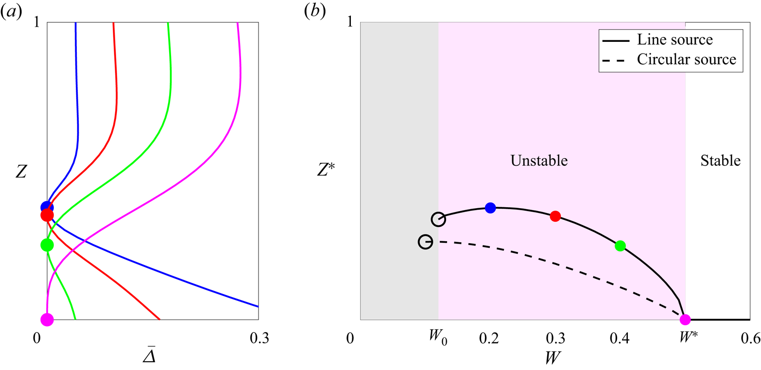
The stability of the system is elucidated by considering the discriminant function (2.32) at leading order,  $\bar {\varDelta }=\bar {\alpha }^2-4\bar {P}_X^2$. As described earlier, for small values of the velocity ratio $W_0< W< W^*$, the discriminant function becomes zero at a critical point $Z=Z^*$ downstream of the inlet. To illustrate this, we have plotted the discriminant function in figure 5(a) for $W=0.2,0.3,0.4,0.5$, and the corresponding critical points $Z^*$ are plotted alongside in figure 5(b). Clearly, $\bar {\Delta }(Z)$ is a non-monotone function that touches zero just once, with critical values in the range $Z^*\in [0,0.37]$ and $Z^*=0$ at $W=W^*$ (also note the corresponding values for the case of a circular source, shown as a dashed line).
(a) Discriminant function  $\bar {\varDelta }$ (steady state), and (b) vertical position of the critical point $Z^*$, where the discriminant equals zero, in the case of a line source. The values of $Z^*$ calculated in the case of a circular source are shown in (b) with a dashed line.
By definition, at the critical point ( $\bar {\Delta }(Z^*)=0$) the shape function $\bar {\alpha }$ and its derivative satisfy
 \begin{gather} \bar{\alpha}(Z^*)= 2\bar{P}_X(1,Z^*), \end{gather}
 \begin{gather}\bar{\beta}(Z^*)={-}\bar{\alpha}(Z^*)^{{-}1}. \end{gather}
Hence, inserting (3.6) and (3.7) into the linearised kinematic condition (3.5) at the critical point  $Z=Z^*$ gives the ordinary differential equation
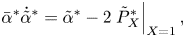 \begin{equation} \bar{\alpha}^*\dot{\tilde{\alpha}}^*=\tilde{\alpha}^*-2\left.\tilde{P}_X^*\right|_{X=1},\end{equation}
where a dot indicates differentiation with respect to time, and  $\ast$ superscripts indicate evaluation at the critical point (e.g. $\tilde {\alpha }^*(T)=\tilde {\alpha }(Z^*,T)$). The stability of the perturbation at the critical point therefore depends on the right-hand side of (3.8), which incidentally is proportional to the perturbed horizontal velocity at the edge of the plume ( $\tilde {\alpha }^*-2\tilde {P}_X^*=2\bar {\alpha }^*\tilde {\mathcal {U}}^*|_{X=1}$), as shown in Appendix C. Hence (3.8) is rewritten as
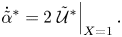 \begin{equation} \dot{\tilde{\alpha}}^*=2\left.\tilde{\mathcal{U}}^*\right|_{X=1}.\end{equation}
To assess the stability, we consider how the sign of the perturbed velocity  $\tilde {\mathcal {U}}|_{X=1}$ relates to the sign of the perturbation $\tilde {\alpha }$ (i.e. whether the shape is deformed inwards or outwards at the critical point).
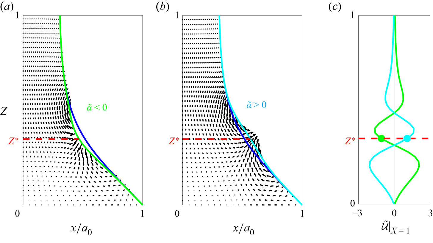
For positive perturbations  $\tilde {\alpha }>0$, the expanded plume shape needs to be filled with fluid, so we expect a net positive velocity perturbation in the vicinity of the critical point, $\tilde {\mathcal {U}}|_{X=1}>0$. Likewise, for negative perturbations $\tilde {\alpha }<0$, a net negative velocity perturbation is required, $\tilde {\mathcal {U}}|_{X=1}<0$, such that the plume can shrink inwards. Hence $\tilde {\mathcal {U}}|_{X=1}$ is positively correlated with $\tilde {\alpha }$, indicating that (3.9) produces unstable solutions that grow unbounded with time when the perturbation is applied close to the critical point. Note, however, that when the perturbation (and therefore the flow) extends far away from the critical point, it is not obvious how $\tilde {\alpha }$ and $\tilde {\mathcal {U}}|_{X=1}$ are correlated.
Next, we demonstrate the existence of a small localised perturbation that grows unbounded over time. To do so we choose a simple Gaussian function for the initial perturbation, which is of the form
 \begin{equation} \tilde{\alpha}(Z^*,0)=\exp\left[ -{(Z-Z^*)^2}/{2\sigma^2} \right],\end{equation}
where  $\sigma$ is the standard deviation. Whilst there are many possible local perturbations that cause instability to occur, we use this one since it is simple and demonstrates the point effectively.
We apply the perturbation (3.10) (using  $\sigma =0.1$) to the case where $W=0.3$ (for which $Z^*=0.35$), and we plot the results in figure 6. Vector fields for the perturbed velocity, $(\tilde {\mathcal {U}},\tilde {\mathcal {W}})$ (see Appendix C for full expressions), are plotted in figures 6(a,b) for the cases of both a positive perturbation $\tilde {\alpha }>0$ and a negative perturbation $\tilde {\alpha }<0$. As shown by the velocity vectors, positive/negative perturbations result in a local flow outwards/inwards from the steady plume shape. Hence the perturbed horizontal velocity $\tilde {\mathcal {U}}|_{X=1}$, which is plotted in figure 6(c), is positive/negative (in the vicinity of the critical point) for positive/negative perturbations, indicating that the solution is unstable.
Vector fields for the perturbed velocity,  $(\tilde {\mathcal {U}},\tilde {\mathcal {W}})$ (see Appendix C), in the cases of both (a) a negative perturbation $\tilde {\alpha }<0$, and (b) a positive perturbation $\tilde {\alpha }>0$. The stability is determined by the sign of the perturbed horizontal velocity at the edge of the plume, $\tilde {\mathcal {U}}|_{X=1}$, which is plotted in (c) for each case. The steady-state plume shape is indicated with a solid blue line in (a,b). The velocity ratio for this case is $W=0.3$, which has a critical point at $Z^*=0.35$.
Whilst this is just a specific case, it nevertheless demonstrates that an infinitesimal solution can be constructed that becomes unstable. Although we do not include the results here, we have also developed a time-dependent implicit numerical scheme that solves the perturbed equations for the pressure and plume shape at first order. These time-dependent numerical simulations confirm that localised perturbations of the form (3.10) become unstable when applied near the critical point. A more detailed eigenvalue analysis could explore the fastest growing perturbation (eigenfunction) and corresponding eigenvalue exponent. However, this lies outside the scope of the current study.
3.2. Moderate velocity ratios $W>W^* \wedge W\approx 1$

Now that we have addressed the case of small velocity ratios, for which the discriminant becomes zero at a critical point, we next address the case of moderate velocity ratios for which  $\varDelta$ is always positive. We restrict our attention to velocity ratios that are larger than $W^*$ but which are still ${O}(1)$ (i.e. ignoring $W\gg 1$). Hence, taking $W\approx 1$, the pressure and the plume shape are well approximated by the expressions (2.22) and (2.23) (which are both ${O}(1-W)$). Meanwhile, the time-dependent kinematic condition (3.1) approximates to
 \begin{equation} -({k}/{\mu})\hat{p}_x\approx \phi a_t + w_b a_z,\quad x\approx a_0.\end{equation}
As before, we consider a small perturbation applied to the plume shape and pressure, but now we avoid converting to dimensionless coordinates for simplicity. Hence we consider a perturbation of the form
 \begin{gather} a=\bar{a}(z)+\epsilon\,\tilde{a}(z,t), \end{gather}
 \begin{gather}\hat{p}=\bar{p}(x,z)+\epsilon\,\tilde{p}(x,z,t). \end{gather}
Attention is required when performing this decomposition, since there are now two small parameters in the problem, namely  $\epsilon >0$ and $\varepsilon =1-W>0$ (we consider $W<1$ without loss of generality). Hence in the following analysis, it is assumed that the perturbation to the shape is relatively much smaller than the perturbation to uniform flow, such that an asymptotic hierarchy $0<\epsilon \ll \varepsilon \ll 1$ is maintained.
After inserting (3.12) and (3.13) into (2.16)–(2.19), (2.21) and (3.11), and expanding in powers of  $\epsilon$, it is clear that the leading-order expressions for the pressure and shape, $\bar {p}$ and $\bar {a}$, are precisely (2.22) and (2.23). Meanwhile, the unsteady terms satisfy
 \begin{equation} -({k}/{\mu})\tilde{p}_x=\phi\tilde{a}_t+w_b\tilde{a}_z,\quad x\approx a_0,\end{equation}
and the pressure perturbation  $\tilde {p}$ satisfies homogeneous versions of the governing equations and boundary conditions (2.16)–(2.19), (2.21) (i.e. with zero on the right-hand sides of all the equations). Hence the pressure perturbation is trivial, $\tilde {p}=0$, and consequently (3.14) also becomes homogeneous. In this way, perturbations to the plume shape $\tilde {a}$ are simply advected downstream with dimensional velocity $w_b/\phi$, and consequently the system is stable.
3.3. A note on the case of large velocity ratios $W>1$

It is worth discussing briefly the plume behaviour in the case where  $W$ is larger than 1, since this has so far been neglected. As discussed earlier, velocity ratios $W>1$ are associated with an expanding plume shape. This expansion requires large horizontal velocities, and hence large values of $-P_X|_{X=1}$, suggesting that the discriminant function (2.32) may become zero or negative for large values of $W$.
$W$.
It is found that the numerical solution of the steady plume shape for  $W>1$ has a sharp gradient near the origin, followed by a slow tapering off. This sharp expansion causes the discriminant to become negative ( $\varDelta <0$) near the origin for velocity ratios larger than $W_n\approx 1.14$ in the case of a line source, and $W_n\approx 1.19$ in the case of a circular source. For $W$ larger than these values, a numerical solution satisfying the steady kinematic condition (2.29) cannot be found. This suggests that a steady plume shape may not be possible, or at least may not take the form of a smooth continuous curve $\alpha (Z)$, as we have prescribed. For example, it is possible that the shape may jump discontinuously from $\alpha (0)=1$ to a larger value near the origin. However, the current modelling approach cannot be used to investigate such scenarios since we require a smooth continuous transformation of the form (2.24a–d).
Whilst further analytical treatment of this case lies outside the scope of this study, it is worth commenting on the validity of the modelling approach for  $W\gg 1$. In such cases, large velocities near the origin may violate the assumptions of Darcy's law. In particular, the Reynolds number of the flow near the origin is given by
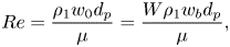 \begin{equation} Re=\frac{\rho_1 w_0 d_p}{\mu}=\frac{W \rho_1 w_b d_p}{\mu}, \end{equation}
where  $d_p$ is the pore size. Since $Re \propto W$, it is expected that inertial effects may become important for $W\gg 1$ (e.g. see Sahu & Flynn Reference Sahu and Flynn2015). Likewise, the Péclet number is also proportional to $W$, indicating that mixing due to dispersion cannot be neglected for $W\gg 1$. Hence, to study the shape and stability of the plume in such scenarios, a more sophisticated model that accounts for laminar flow and dispersive mixing might be more appropriate than the linear stability analysis based on Darcy's law used here.
3.4. Further cases and considerations
We have therefore shown that plume shapes are stable in the regime  $W\approx 1$, and unstable in the regime $W_0< W< W^*$. It is not known whether the plume shapes for $W>W^*$ but $W\not \approx 1$ are stable or unstable (e.g. one could argue that $W=0.6\not \approx 1$), and for this a full eigenvalue analysis is required. Such an analysis could predict the largest value of $W$ that onsets instability (i.e. producing a positive real-valued eigenvalue). However, for the purposes of this study, and since our experimental data suggest a stable shape for velocity ratios as small as $W=0.58$ (see figure 3a), this analysis covers the relevant and interesting range of cases.
To go beyond the current analysis and resolve the nonlinear instability at very small velocity ratios  $W< W_0$, a time-dependent numerical simulation is required in either two or three dimensions (e.g. see Hewitt et al. Reference Hewitt, Neufeld and Lister2013b; Hewitt & Lister Reference Hewitt and Lister2017). In particular, it is not clear exactly how the flow evolves over time, whether it forms fingers, filaments or disconnected regions. Moreover, in the presence of dispersion, it is likely that thin disconnected regions may fuse together. It is possible that the stability diagram in figures 2(b) and 4(b) may not be complete, but in fact could contain other stable, unstable or periodic branches. Hence such a numerical simulation could be used to explore the full range of solution branches, and classify any bifurcation points, such as at $W=W_0$, that may be a fold (saddle node) or a Hopf bifurcation.
As described earlier, it is worth commenting briefly on the effects of the ambient fluid in the unsteady case. In particular, in the above analysis we have assumed implicitly (i.e. via the dynamic boundary condition (2.10)) that the injected fluid and the ambient fluid are decoupled. However, in the unsteady case (unlike the steady case) the ambient fluid is not quiescent. In fact, as the plume expands or contracts over time, the ambient fluid must be displaced accordingly. However, as long as the perturbation to the plume shape has a sufficiently large aspect ratio, the rearrangement of the ambient fluid should not affect the plume growth to good approximation. This is similar to the shallow-water approximation used for gravity currents in porous media (Huppert & Woods Reference Huppert and Woods1995), for which the injected fluid is not coupled to the ambient fluid so long as the aspect ratio of the current remains large.
This argument does not extend to the case where the viscosity of the injected fluid is different to that of the ambient fluid. In this case, the viscosity contrast affects the pressure gradients on either side of the perturbation to the interface as it grows. If  $M=\mu _1/\mu _2$ denotes the viscosity contrast between injected and ambient fluids, then the interface becomes destabilised for $M<1$ and stabilised for $M>1$, as described in the famous study by Saffman & Taylor (Reference Saffman and Taylor1958). For this reason, we do not expect the results of § 3 to apply in the case where $M\neq 1$.
4. Discussion and perspectives
We have studied the shape and stability of buoyancy-driven plumes near their injection point within a porous medium. The key controlling parameter is the ratio between the inlet velocity and the far-field (buoyancy) velocity. Whether this ratio is larger or smaller than 1 determines whether the plume is expanding or contracting downstream. For small values of this ratio, the plume shape becomes unstable at a critical point downstream, which we have demonstrated using a linear stability analysis. On the other hand, when the velocity ratio is close to 1, we have shown that the plume shape is stable.
Future work could include the effects of mixing between the injected fluid and the ambient fluid, similarly to Sahu & Flynn (Reference Sahu and Flynn2015) and Lyu & Woods (Reference Lyu and Woods2016). In particular, as the two fluids mix together, the difference in density between them becomes smaller. Hence buoyancy decreases and the width of the plume increases as the flow moves downstream. As described earlier, in § 2, the experiments of Sahu & Flynn (Reference Sahu and Flynn2015) indicated that mixing takes place over vertical length scales  ${\sim }10$ times larger than the plume width, whereas we have shown that the near-field shape adjusts within length scales close to ${\sim }1$ times the plume width (e.g. see figures 2 and 4). Hence we have confirmed that dispersion occurs at larger length scales than the adjustments to the plume shape studied here in the near field.
A future study could extend this work to account for multiphase effects in the case of immiscible fluids. In such scenarios, the effects of surface tension between phases are represented by the capillary pressure and relative permeability functions for each phase (Woods Reference Woods2015). As shown by the famous study of Buckley & Leverett (Reference Buckley and Leverett1942) for displacement flows, capillary pressure tends to smooth out the sharp interface between phases. Hence one would expect this to cause the plume to widen as it moves downstream. As it does so, the saturation would have to decrease (to conserve mass) and therefore the relative permeability would also decrease, causing the plume to slow down. However, it is not clear exactly what shape the two-phase plume would take, or how this affects the near-field stability.
It would also be interesting to investigate the possible effects of a time-varying injection  $Q(t)$ (Huppert Reference Huppert1982). In particular, it may be possible to stabilise/destabilise the near-field plume shape by controlling dynamically the flow rate appropriately. In this case, the time scale for changes in flow rate scales like $t\sim Q/\dot {Q}$, whereas the time scale for buoyancy is $t\sim a_0\phi /w_b$. Hence we require sufficiently large values of $a_0\phi \dot {Q}/w_bQ$ to be able to regulate the flow in this way.
It is worth noting the relevance of this study to the case of CO $_2$ sequestration, in which buoyant CO $_2$ (originating from emissions due to power plants and industrial processes) is injected into subsurface geological aquifers for storage. In this case, low-permeability sedimentary layers may cause the CO $_2$ to spread out as it rises (Bickle et al. Reference Bickle, Chadwick, Huppert, Hallworth and Lyle2007; Cowton et al. Reference Cowton, Neufeld, White, Bickle, White and Chadwick2016, Reference Cowton, Neufeld, White, Bickle, Williams, White and Chadwick2018). It is important to be able to quantify the behaviour of the buoyant CO $_2$ if and when it penetrates through these low-permeability layers and migrates further upwards. Hence our study provides a tool for modelling the flow behaviour near the breakthrough locations (as well as near injection points, in general), which is useful for quantifying leakage rates (Gilmore et al. Reference Gilmore, Sahu, Benham, Neufeld and Bickle2022) and the consequent CO $_2$ migration speeds (Neufeld, Vella & Huppert Reference Neufeld, Vella and Huppert2009). Moreover, the stability of the plume determines how it mixes with the surrounding brine (i.e. by breaking apart into filaments, fingers or disconnected regions), thereby influencing how it becomes trapped due to dissolution and residual trapping (Nordbotten & Celia Reference Nordbotten and Celia2011; Krevor et al. Reference Krevor, Blunt, Benson, Pentland, Reynolds, Al-Menhali and Niu2015). However, in such cases, there are other more complicated physical phenomena to account for, such as the dissolution of the CO $_2$ (MacMinn et al. Reference MacMinn, Neufeld, Hesse and Huppert2012), multiphase effects (Golding et al. Reference Golding, Neufeld, Hesse and Huppert2011) and flow rearrangement due to geological heterogeneities (Benham, Bickle & Neufeld Reference Benham, Bickle and Neufeld2021a,Reference Benham, Bickle and Neufeldb).
When applying this study to such real injection scenarios, it is important to acknowledge the possible limitations of our simple modelling approach. For example, the stability analysis in § 3 is restricted to the case where there is no viscosity contrast between the injected and ambient fluids ( $M=1$). However, in the context of CO $_2$ sequestration, $M$ can be as small as $1/20$ or $1/30$ (Bickle et al. Reference Bickle, Kampman, Chapman, Ballentine, Dubacq, Galy, Sirikitputtisak, Warr, Wigley and Zhou2017), which is likely to make the plume more unstable due to the Saffman–Taylor instability. Furthermore, our modelling of the input conditions as a line source or a circular source is idealised compared to real injection scenarios, where CO $_2$ spreads out as a fully three-dimensional plume. Modelling such scenarios is difficult because a coordinate transformation of the form (2.24a–d), (2.35), may not be possible. Hence it is expected that a three-dimensional time-dependent simulation would be required to address such flows, similar to Hewitt & Lister (Reference Hewitt and Lister2017). However, in the case where the stable shape is known, a linear stability analysis (similar to § 3) may be possible.
Acknowledgements
The author would like to thank K.A. Gilmore for supplying the experimental photographs and further information regarding the experiments. The author would also like to thank the three anonymous peer reviewers for helping to improve this paper with useful comments and suggestions.
Declaration of interests
The author reports no conflict of interest.
Appendix A. Derivation of the steady-state solution for a circular source
In this appendix, we describe the derivation of the pressure solution (2.33) described in § 2.4. We start by seeking a solution to the Darcy equations and boundary conditions (2.4)–(2.10) (in cylindrical radial coordinates) of the form (2.11)–(2.13). In the case where the inlet velocity is close to the buoyancy velocity ( $W\approx 1$), the equations are linearised and the boundary conditions (2.9)–(2.10) are imposed at $r=a_0$. In this way, the hatted pressure solves the linear system
 \begin{gather} \hat{p}_{zz}+\hat{p}_r/r+\hat{p}_{rr}=0, \end{gather}
 \begin{gather}\hat{p}_r=0,\quad r=0, \end{gather}
 \begin{gather}\hat{p}_z={\rm \Delta}\rho\,g(1-W),\quad z=0, \end{gather}
 \begin{gather}\hat{p}_z\rightarrow 0,\quad z\rightarrow \infty, \end{gather}
 \begin{gather}\hat{p}_r={-}{\rm \Delta} \rho\,g\,a'(z),\quad r=a_0, \end{gather}
 \begin{gather}\hat{p}=0,\quad r=a_0, \end{gather}
which is derived in a similar manner to (2.16)–(2.21). Notice how the above system can be solved independently of the linearised kinematic condition (A5). Once the solution is found, (A5) can be used to calculate the shape  $a(z)$.
The solution to (A1)–(A4), (A6) is found by seeking a separable solution of the form  $\hat {p}(r,z)=F(r)\,G(z)$. Inserting this into Laplace's equation (A1) and dividing by $FG$ leads to
 \begin{equation} F''(r)/F(r)+F'(r)/r\,F(r)={-}G''(z)/G(z)={-}\lambda^2,\end{equation}
for some real eigenvalue  $\lambda$. By switching to variables $\xi =\lambda r$, $\mathcal {F}(\xi )=F(r)$, the radial part of (A7) is rewritten as
 \begin{equation} \xi^2\,\mathcal{F}''(\xi)+\xi\,\mathcal{F}'(\xi)+\xi^2\,\mathcal{F}(\xi)=0, \end{equation}
which is Bessel's equation with index  $0$. The general solution is
 \begin{equation} \mathcal{F}=C\,J_0(\xi)+D\,Y_0(\xi), \end{equation}
where  $J_0$ and $Y_0$ are zero-order Bessel functions of the first and second kinds, and $C$ and $D$ are some constants. The symmetry boundary condition (A2) indicates that $D=0$, whilst the dynamic condition (A6) gives
 \begin{equation} J_0(a_0\lambda)=0.\end{equation}
There are infinitely many solutions to (A10), producing a sequence of eigenvalues
 \begin{equation} \lambda_n=j_{0,n}/a_0,\quad n=1,2,\ldots, \end{equation}
where  $j_{0,n}$ is the $n\mathrm {th}$ zero of $J_0$. For each eigenvalue, there is a corresponding coefficient $C_n$, which will be determined by looking at the axial component of the pressure $G(z)$.
The axial component of (A7) is rewritten as
 \begin{equation} G''(z)-\lambda^2\,G(z)=0, \end{equation}
which has exponentially growing and decaying solutions. Since (A4) indicates that  $G'(z)\rightarrow 0$ as $z\rightarrow \infty$, only exponentially decaying solutions are permitted. Hence the separable solution is given by the infinite sum
 \begin{equation} \hat{p}=\sum_{n=1}^\infty C_n\,J_0(j_{0,n}r/a_0) \exp({-j_{0,n}z/a_0}).\end{equation}
The coefficients  $C_n$ are determined by applying the boundary condition (A3), which becomes
 \begin{equation} \sum_{n=1}^\infty -\frac{j_{0,n}C_n}{a_0}\,J_0(j_{0,n}r/a_0) ={\rm \Delta}\rho\,g(1-W). \end{equation}
By multiplying each side by  $r\,J_0(j_{0,m}r/a_0)$ (for some $m$) and integrating (using the orthogonality properties of Bessel functions), we get
 \begin{equation} -\frac{j_{0,m}C_m}{a_0} \int_0^{a_0} r\,J_0(j_{0,m}r/a_0)^2\,\mathrm{d}r = {\rm \Delta}\rho\,g(1-W) \int_0^{a_0} r\,J_0(j_{0,m}r/a_0)\,\mathrm{d}r, \end{equation}
which simplifies to
 \begin{equation} -\frac{j_{0,m}C_m}{a_0}\,\frac{a_0^2\,J_1(j_{0,m})^2}{2} = {\rm \Delta}\rho\,g(1-W)\, \frac{a_0^2\,J_1(j_{0,m})}{j_{0,m}} . \end{equation}
After simplification, this gives
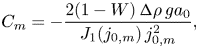 \begin{equation} C_m={-} \frac{2(1-W)\,{\rm \Delta}\rho\,g a_0}{J_1(j_{0,m})\,j_{0,m}^2}, \end{equation}
which leads to (2.33) precisely.
Appendix B. First-order pressure perturbation
In this appendix, we describe briefly the system of equations required to calculate the first-order pressure perturbation, which is used to analyse stability in § 3.1. After inserting the decomposition (3.3)–(3.4) into the governing equation for the pressure (2.25), and linearising in terms of the small parameter  $\epsilon \ll 1$, the corrected equation at first order is
 \begin{equation} A_{XX}\tilde{P}_{XX} +A_{XZ}\tilde{P}_{XZ}+ A_{ZZ} \tilde{P}_{ZZ} + A_X\tilde{P}_X =B_{ZZ}\tilde{\alpha}_{ZZ} +B_Z\tilde{\alpha}_Z + B\tilde{\alpha}, \end{equation}
where the coefficients (using subscript notation for clarity) are given by
 \begin{gather} A_{XX}=\bar{\alpha}^{{-}1}(1 + \bar{\alpha}^2 \bar{\beta}^2 X^2), \end{gather}
 \begin{gather}A_{XZ}={-} 2 \bar{\alpha} \bar{\beta} X, \end{gather}
 \begin{gather}A_{ZZ}= \bar{\alpha}, \end{gather}
 \begin{gather}A_X=\bar{\alpha}X (\bar{\beta}^2 - \bar{\alpha} \bar{\beta}' ), \end{gather}
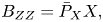 \begin{gather}B_{ZZ}=\bar{P}_{X} X, \end{gather}
 \begin{gather}B_Z={-}2 X (2 \bar{\beta} \bar{P}_X - \bar{P}_{XZ} + \bar{\beta} \bar{P}_{XX} X), \end{gather}
 \begin{gather}B={-}\bar{\alpha}^{{-}2} \left[\bar{\alpha}^2 ({-}3 \bar{\beta}^2 \bar{P}_X + \bar{\beta}' \bar{P}_X + 2 \bar{\beta} \bar{P}_{XZ}) X - 2 \bar{P}_{XX} (1 + \bar{\alpha}^2 \bar{\beta}^2 X^2)\right]. \end{gather}
Likewise, the boundary conditions (2.26)–(2.28), (2.30), linearised and keeping only first-order terms, become
 \begin{gather} \tilde{P}_X=0,\quad X=0, \end{gather}
 \begin{gather}\tilde{P}_Z-X\bar{\beta} \tilde{P}_X=\bar{P}_X X\bar{\alpha}^{{-}1} (\tilde{\alpha}_Z-\bar{\beta}\tilde{\alpha}),\quad Z=0, \end{gather}
 \begin{gather}\tilde{P}_Z-X\bar{\beta} \tilde{P}_X\rightarrow \bar{P}_X X \bar{\alpha}^{{-}1}( \tilde{\alpha}_Z-\bar{\beta}\tilde{\alpha}),\quad Z\rightarrow \infty, \end{gather}
 \begin{gather}\tilde{P}=0,\quad X=1. \end{gather}
The new system of equations is solved together (using the same finite difference scheme described earlier) with the linearised kinematic boundary condition (3.5) to acquire the first-order pressure and shape  $\tilde {P},\tilde {\alpha }$.
Appendix C. First-order velocity perturbation
In this appendix, we derive briefly expressions for the perturbed velocity field that are used to create the vector fields in figure 6. Following the notation used in § 2.2, the dimensionless flow velocities are given by
 \begin{gather} \hat{u}/w_b={-} \alpha^{{-}1}{P}_X, \end{gather}
 \begin{gather}\hat{w}/w_b={-}{P}_Z+X\alpha'\alpha^{{-}1}{P}_X. \end{gather}
Next, we insert (3.3) and (3.4) into (C1)–(C2), and expand in powers of  $\epsilon$, keeping only leading-order and first-order terms. We denote the leading-order velocities as $\bar {\mathcal {U}},\bar {\mathcal {W}}$, and the first-order velocities as $\tilde {\mathcal {U}},\tilde {\mathcal {W}}$. These are given by
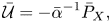 \begin{gather} \bar{\mathcal{U}}={-} \bar{\alpha}^{{-}1}\bar{P}_X, \end{gather}
 \begin{gather}\bar{\mathcal{W}}={-}\bar{P}_Z+X\bar{\beta}\bar{P}_X, \end{gather}
 \begin{gather}\tilde{\mathcal{U}}=\bar{\alpha}^{{-}2}\left[\tilde{\alpha}\bar{P}_X-\bar{\alpha}\tilde{P}_X\right], \end{gather}
 \begin{gather}\tilde{\mathcal{W}}={-}\tilde{P}_Z + \left[(-\bar{\beta}\tilde{\alpha} + \tilde{\alpha}_Z) \bar{P}_X\bar{\alpha}^{{-}1} + \bar{\beta} \tilde{P}_X\right] X. \end{gather}
The final two expressions, (C5) and (C6), are precisely the terms used to plot the perturbed velocity vector field in figure 6.
It should be noted that at the critical point  $X=1$, $Z=Z^*$, the above equations simplify to
 \begin{gather} \bar{\mathcal{U}}={-} 1/2, \end{gather}
 \begin{gather}\bar{\mathcal{W}}={-}1/2, \end{gather}
 \begin{gather}\tilde{\mathcal{U}}=(2\bar{\alpha})^{{-}1}\left[\tilde{\alpha}-2\tilde{P}_X\right], \end{gather}
 \begin{gather}\tilde{\mathcal{W}}= (\bar{\alpha}^{{-}1}\tilde{\alpha} + \tilde{\alpha}_Z)/2 -\bar{\alpha}^{{-}1} \tilde{P}_X. \end{gather}
Hence we see that the horizontal velocity perturbation (C9) is proportional to the right-hand side of (3.8).


 Open access

