


 ) which unify these currently disconnected endeavours. Coupling the segregation with the flow, and
1. Introduction
Despite nearly all natural and man-made granular materials being composed of grains of varying size, shape and frictional properties, the majority of continuum flow modelling has largely been restricted to perfectly monodisperse aggregates. The purpose of this work is therefore to extend the current granular flow models by introducing multiple phases, with different properties, and to model inter-phase segregation. Coupling the flow rheology to the local constituent concentrations is important because the mobility of a granular flow is strongly affected by the local frictional properties of the grains. In turn, the bulk flow controls the strength and direction of the segregation as well as the advection of the granular phases.
Striking examples of segregation induced feedback on the bulk flow are found during levee formation (Iverson & Vallance Reference Iverson and Vallance2001; Johnson et al. Reference Johnson, Kokelaar, Iverson, Logan, LaHusen and Gray2012; Kokelaar et al. Reference Kokelaar, Graham, Gray and Vallance2014) and fingering instabilities (Pouliquen, Delour & Savage Reference Pouliquen, Delour and Savage1997; Pouliquen & Vallance Reference Pouliquen and Vallance1999; Woodhouse et al. Reference Woodhouse, Thornton, Johnson, Kokelaar and Gray2012; Baker, Johnson & Gray Reference Baker, Johnson and Gray2016b), which commonly occur during the run-out of pyroclastic density currents, debris flows and snow avalanches. Many other examples of segregation–flow coupling occur in industrial settings (Williams Reference Williams1968; Gray & Hutter Reference Gray and Hutter1997; Makse et al. Reference Makse, Havlin, King and Stanley1997; Hill et al. Reference Hill, Khakhar, Gilchrist, McCarthy and Ottino1999; Ottino & Khakhar Reference Ottino and Khakhar2000; Zuriguel et al. Reference Zuriguel, Gray, Peixinho and Mullin2006). Storage silo filling and emptying, stirring mixers and rotating tumblers all have the common features of cyclic deformation and an ambition of generating well-mixed material. However, experiments consistently suggest that these processes have a tendency to promote local segregation, which can feedback on the bulk flow velocities. Considering the inherent destructive potential of geophysical phenomena and the implications of poor efficiency in industrial mixing, a continuum theory which captures the important physics of flow and of segregation simultaneously is therefore highly desirable.
To date, the leading approaches for solving coupled flow and segregation have come from either discrete particle simulations (Tripathi & Khakhar Reference Tripathi and Khakhar2011; Thornton et al. Reference Thornton, Weinhart, Luding and Bokhove2012) or from depth-averaged equations (Woodhouse et al. Reference Woodhouse, Thornton, Johnson, Kokelaar and Gray2012; Baker et al. Reference Baker, Johnson and Gray2016b; Viroulet et al. Reference Viroulet, Baker, Rocha, Johnson, Kokelaar and Gray2018). Particle simulations, using the discrete element method (DEM), provide important rheological information as evolving velocities, stresses and constituent concentrations can be directly computed given only minimal approximations. Such results can then be used to motivate models for the bulk flow (GDR MiDi 2004; Jop, Forterre & Pouliquen Reference Jop, Forterre and Pouliquen2006; Singh et al. Reference Singh, Magnanimo, Saitoh and Luding2015) and also to form connections between flow and segregation processes (Hill & Fan Reference Hill and Fan2008; Staron & Phillips Reference Staron and Phillips2015). Unfortunately, the discrete particle approach is naturally limited by computational expense as many flows of interest include such a large number of particles that direct DEM calculations are unfeasible. Recently efforts have been made to overcome this limitation with the development of hybrid schemes (e.g. Yue et al. Reference Yue, Smith, Chen, Chantharayukhonthorn, Kamrin and Grinspun2018; Xiao et al. Reference Xiao, Fan, Jacob, Umbanhowar, Kodam, Koch and Lueptow2019) which couple discrete particle dynamics to continuum solvers, but these approaches naturally invoke additional complexity and new assumptions are required in order to map properly and consistently between the somewhat disparate approaches.
Depth-averaged models, which reduce the full three-dimensional flow to two dimensions by integrating though the depth and assuming shallowness, lead to efficient numerical codes which are widely used in geophysical modelling (see e.g. Grigorian, Eglit & Iakimov Reference Grigorian, Eglit and Iakimov1967; Savage & Hutter Reference Savage and Hutter1989; Iverson Reference Iverson1997; Gray, Wieland & Hutter Reference Gray, Wieland and Hutter1999; Pouliquen & Forterre Reference Pouliquen and Forterre2002; Sheridan et al. Reference Sheridan, Stinton, Patra, Pitman, Bauer and Nichita2005; Mangeney et al. Reference Mangeney, Bouchut, Thomas, Vilotte and Bristeau2007; Christen, Kowalski & Bartelt Reference Christen, Kowalski and Bartelt2010; Gray & Edwards Reference Gray and Edwards2014; Delannay et al. Reference Delannay, Valance, Mangeney, Roche and Richard2017; Rauter & Tuković Reference Rauter and Tuković2018; Rocha, Johnson & Gray Reference Rocha, Johnson and Gray2019). However, depth-averaged approaches are limited to geometries in which there is a clear dimension that remains shallow throughout the dynamics. This approximation holds well for thin flows on inclined planes and for flows over certain gradually varying terrain, but breaks down in many flows of practical interest, such as those in hoppers, silos and rotating drums.
Historical attempts to construct three-dimensional continuum models for monodisperse granular materials focused on quasi-static deformations and lead to elasto-plastic formulations of models such as the Drucker–Prager yield condition (Lubliner Reference Lubliner2008) and critical state soil mechanics (Schofield & Wroth Reference Schofield and Wroth1968). Despite successes in modelling the point of failure of materials under load, calculations of the subsequent time-dependent flow proved to be problematic, because the results are grid-size dependent. Schaeffer (Reference Schaeffer1987) showed that this was because the underlying equations are mathematically ill posed, i.e. in the small wavelength limit the growth rate of linear instabilities becomes unbounded in certain directions.
Despite the Mohr–Coulomb/Drucker–Prager plasticity theory being designed for the flow of monodisperse grains, the grain diameter  $d$ does not appear in the constitutive model. It can be incorporated by making the friction $\mu$ a function of the non-dimensional inertial number, which is defined as
 \begin{equation} I = \frac{d \dot{\gamma}}{\sqrt{p/\rho_*}}, \end{equation}
where  $\dot \gamma$ is the shear rate, $p$ is the pressure and $\rho _*$ is the intrinsic grain density (Savage Reference Savage1984; Ancey, Coussot & Evesque Reference Ancey, Coussot and Evesque1999; GDR MiDi 2004). Jop et al. (Reference Jop, Forterre and Pouliquen2006) generalized the scalar $\mu (I)$-rheology to tensorial form. The resultant incompressible $\mu (I)$-rheology leads to a significantly better posed system of equations (Barker et al. Reference Barker, Schaeffer, Bohorquez and Gray2015). For the $\mu (I)$ curve suggested by Jop, Forterre & Pouliquen (Reference Jop, Forterre and Pouliquen2005), the equations are well posed for a large range of intermediate values of $I$ and are only ill posed for very low or relatively high inertial numbers.
Barker & Gray (Reference Barker and Gray2017) derived a new functional form for the  $\mu (I)$ relation, which is known as the partially regularized $\mu (I)$-rheology. This ensures well posedness for $0<I<I_{max}$, where $I_{max}$ is a very large value, and leads to stable and reliable numerical schemes. It also provides a better fit to experimental (Holyoake & McElwaine Reference Holyoake and McElwaine2012; Barker & Gray Reference Barker and Gray2017) and DEM data (Kamrin & Koval Reference Kamrin and Koval2012) than the original $\mu (I)$ curve, but also introduces a creep state (i.e. $\mu =0$ when $I=0$) so the granular material no longer has a yield stress. It is possible to formulate well-posed models with a yield stress by introducing bulk compressibility (Barker et al. Reference Barker, Schaeffer, Shearer and Gray2017; Schaeffer et al. Reference Schaeffer, Barker, Tsuji, Gremaud, Shearer and Gray2019) or non-locality (Henann & Kamrin Reference Henann and Kamrin2013). However, in this paper the partially regularized $\mu (I)$-rheology is chosen for the bulk flow, both for simplicity and because it is most readily compatible with existing numerical methods and particle segregation models.
Initially well-mixed granular materials have a strong propensity of ordering spatially when they undergo flow. Chief among these effects is that of particle-size segregation, made famous through the moniker ‘the Brazil nut effect’ (Rosato et al. Reference Rosato, Strandburg, Prinz and Swendsen1987), whereby particles move relative to the bulk flow based on their size compared with their neighbours. The resultant vertical distribution, in which larger particles are often concentrated at the surface of a flow, can also be observed in many geophysical mass flows, forming so-called inversely graded deposits (e.g. Middleton Reference Middleton1970; Festa et al. Reference Festa, Ogata, Pini, Dilek and Codegone2015). The origin of this effect was explained through statistical entropic arguments by Savage & Lun (Reference Savage and Lun1988) who proposed a means of ‘kinetic sieving’ (Middleton Reference Middleton1970) in which smaller grains are more likely to fall (by gravity) into voids that are created as layers of particles are sheared over one another. Force imbalances then drive particles out of the denser layer, which is known as ‘squeeze expulsion’. The combination of kinetic sieving and squeeze expulsion produces a net upward motion of large particles as the smaller grains percolate downwards. These concepts formed the basis of the theory of Gray & Thornton (Reference Gray and Thornton2005) who focused on this form of gravity-driven segregation in granular free-surface flows. The theory was later extended by Gray & Chugunov (Reference Gray and Chugunov2006), in order to account for diffusive mixing, and has been successfully applied to a range of gravity-driven flows (Gray Reference Gray2018). However, Fan & Hill (Reference Fan and Hill2011) found that the direction of segregation was not always aligned with the vector of gravitational acceleration. Instead gradients in kinetic stress were found to drive and orient segregation in a range of geometries (Hill & Tan Reference Hill and Tan2014). These findings have since inspired many investigations into the micromechanical origin of size segregation (Staron & Phillips Reference Staron and Phillips2015; Guillard, Forterre & Pouliquen Reference Guillard, Forterre and Pouliquen2016; van der Vaart et al. Reference van der Vaart, van Schrojenstein Lantman, Weinhart, Luding, Ancey and Thornton2018), but a unified and compelling theory is still lacking.
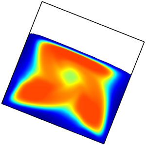
In order to accommodate different models for size segregation and different flow rheologies, this paper first introduces a very general framework for multi-component flows in § 2. In particular, the multicomponent segregation theory of Gray & Ancey (Reference Gray and Ancey2011) is generalized to allow sub-mixtures to segregate in different directions and with differing diffusion rates. In § 3 the three primary coupling mechanisms are discussed in detail. Section 4 documents the general numerical method, which is then extensively tested against the one-way coupled simulations in § 5. Two-way fully coupled simulations are then presented for flow down an inclined plane, in § 6, and in § 7 simulations are performed for a square rotating drum. The new experimental segregation law of Trewhela, Ancey & Gray (Reference Trewhela, Ancey and Gray2021) is tested against the steady-state DEM solutions of Tripathi & Khakhar (Reference Tripathi and Khakhar2011) in § 6.3 and then used in § 7 for the rotating drum simulations, which are able to spontaneously generate petal-like patterns that have previously been seen in the experiments of Hill et al. (Reference Hill, Khakhar, Gilchrist, McCarthy and Ottino1999), Ottino & Khakhar (Reference Ottino and Khakhar2000) and Mounty (Reference Mounty2007).
2. Governing equations
2.1. The partially regularized  $\mu (I)$-rheology for the bulk flow

The granular material is assumed to be composed of a mixture of particles that may differ in size, shape and surface properties, but have the same intrinsic particle density  $\rho _*$. If the solids volume fraction $\varPhi$ is constant, which is a reasonable first approximation (GDR MiDi 2004; Tripathi & Khakhar Reference Tripathi and Khakhar2011; Thornton et al. Reference Thornton, Weinhart, Luding and Bokhove2012), then the bulk density $\rho =\varPhi \rho _*$ is constant and uniform throughout the material. Mass balance then implies that the bulk velocity field $\boldsymbol {u}$ is incompressible
 \begin{equation} \boldsymbol{\nabla} \boldsymbol{\cdot} \boldsymbol{u} = 0, \end{equation}
where  $\boldsymbol {\nabla }$ is the gradient and $\boldsymbol {\cdot }$ is the dot product. The momentum balance is
 \begin{equation} \rho\left(\frac{\partial\boldsymbol{u}}{\partial t}+\boldsymbol{u}\boldsymbol{\cdot}\boldsymbol{\nabla}\boldsymbol{u}\right) = -\boldsymbol{\nabla} p + \boldsymbol{\nabla} \boldsymbol{\cdot} \left(2\eta\boldsymbol{D}\right) + \rho \boldsymbol{g}, \end{equation}
where  $p$ is the pressure, $\eta$ is the viscosity, $\boldsymbol {D} = (\boldsymbol {\nabla } \boldsymbol {u} + (\boldsymbol {\nabla } \boldsymbol {u})^{T})/2$ is the strain-rate tensor and $\boldsymbol {g}$ is the gravitational acceleration. Assuming alignment of the shear-stress and strain-rate tensors the $\mu (I)$-rheology (Jop et al. Reference Jop, Forterre and Pouliquen2006) implies that the granular viscosity is
 \begin{equation} \eta = \frac{\mu(I) p}{2\|\boldsymbol{D}\|}, \end{equation}
where the second invariant of the strain-rate tensor is defined as
 \begin{equation} \|\boldsymbol{D}\| = \sqrt{\frac{1}{2} \text{tr}(\boldsymbol{D}^{2})}, \end{equation}
and the inertial number, defined in (1.1), in this notation becomes
 \begin{equation} I = \frac{2d \|\boldsymbol{D}\|}{\sqrt{p/\rho_*}}. \end{equation}
The meaning of the particle size  $d$ in a polydisperse mixture will be clarified in § 3.2. Note that this paper is restricted to two-dimensional deformations with an isotropic Drucker–Prager yield surface. However, as shown by Rauter, Barker & Fellin (Reference Rauter, Barker and Fellin2020), this framework can be extended to include three-dimensional deformations through further modification of the granular viscosity i.e. dependence on $\det (\boldsymbol {D})$.
The viscosity (2.3) is a highly nonlinear function of the inertial-number-dependent friction  $\mu =\mu (I)$, pressure $p$ and the second invariant of the strain rate $\|\boldsymbol {D}\|$. Barker et al. (Reference Barker, Schaeffer, Bohorquez and Gray2015) examined the linear instability of the system, to show that the growth rate becomes unbounded in the high wavenumber limit, and hence the incompressible $\mu (I)$-rheology is mathematically ill posed, when the inequality
 \begin{equation} 4\left(\frac{I \mu^{\prime}}{\mu}\right)^{2} -4\left(\frac{I \mu^{\prime}}{\mu}\right)+\mu^{2}\left(1-\frac{I \mu^{\prime}}{2\mu} \right) > 0, \end{equation}
is satisfied, where  $\mu ^{\prime }=\partial \mu /\partial I$. Ill posedness of this type is not only unphysical, but results in two-dimensional time-dependent numerical computations that do not converge with mesh refinement (see e.g. Barker et al. Reference Barker, Schaeffer, Bohorquez and Gray2015; Barker & Gray Reference Barker and Gray2017; Martin et al. Reference Martin, Ionescu, Mangeney, Bouchut and Farin2017). If the friction is not inertial number dependent ( $\mu =\text {const.}$) the ill-posedness condition (2.6) is satisfied for all inertial numbers and the system of equations is always ill posed (Schaeffer Reference Schaeffer1987). The equations are also ill posed if the friction $\mu$ is a decreasing function of $I$, since all the terms in (2.6) are strictly positive.
The original form of the  $\mu (I)$-curve proposed by Jop et al. (Reference Jop, Forterre and Pouliquen2005) is a monotonically increasing function of $I$ starting at $\mu _{s}$ at $I=0$ and asymptoting to $\mu _{d}$ at large $I$,
$I$,
 \begin{equation} \mu(I) = \frac{\mu_{s} I_{0}+\mu_{d} I}{I_{0}+I}, \end{equation}
where  $I_{0}$ is a material specific constant. The inertial number dependence in (2.7) gives the rheology considerably better properties than the original, constant friction coefficient, Mohr–Coulomb/Drucker–Prager theory. Provided $\mu _{d}-\mu _{s}$ is large enough, the system is well-posed when the inertial number lies in a large intermediate range of inertial numbers $I\in [I_1^{N},I_2^{N}]$. The equations are, however, ill posed if either the inertial number is too low $I<I_1^{N}$ or too high $I>I_2^{N}$, or if $\mu _{d}-\mu _{s}$ is not large enough. For the parameter values given in table 1 the $\mu (I)$ rheology is well posed for $I\in [0.00397, 0.28016]$.
Table 1. The frictional parameters  $\mu _s$, $\mu _d$, $\mu _{\infty }$, $I_0$ and $\alpha$ in Barker & Gray's (Reference Barker and Gray2017) friction law, which were measured for $143\ \mathrm {\mu }\textrm {m}$ glass beads. The value $I_1\simeq I_1^{N}$ is set by the lower bound for well posedness in Jop et al.'s (Reference Jop, Forterre and Pouliquen2006) friction law using the parameters above. Unless stated otherwise, the remaining parameters are the values chosen in the numerical simulations. Note that the air viscosity is higher than the physical value of $\eta _*^{a}=1.81\times 10^{-5}\ \textrm {kg}\,(\textrm {ms})^{-1}$ to prevent the convective Courant number limiting the time-step size.

The range of well posedness was extended by Barker & Gray (Reference Barker and Gray2017) to  $0\leq I \leq I_{max}$, where $I_{max}$ is a large maximal value, by changing the shape of the $\mu (I)$-curve. This paper uses the $\mu (I)$-curve proposed by Barker & Gray (Reference Barker and Gray2017)
 \begin{equation} \mu = \begin{cases} \displaystyle \sqrt{\frac{\alpha}{\log\left(\dfrac{A}{I}\right)}}, & \text{for } I \leq I_1,\\ \displaystyle \frac{\mu_{s} I_{0}+\mu_{d} I+\mu_{\infty} I^{2}}{I_{0}+I}, & \text{for } I > I_1, \end{cases} \end{equation}
where  $\alpha$ and $\mu _{\infty }$ are new material constants and
 \begin{equation} A=I_1\exp\left(\frac{\alpha(I_0+I_1)^{2}}{(\mu_s I_0 + \mu_d I_1 + \mu_{\infty} I_1^{2})^{2}}\right), \end{equation}
is chosen to ensure continuity between the two branches at  $I=I_1$. As shown in figure 1 this curve stays close to (2.7) in the well-posed region of parameter space, but passes though $\mu =0$ at $I=0$ and is asymptotically linear in $I$ at large inertial numbers. For the parameters given in table 1, the matching occurs at $I_1=0.004$ (which is very slightly larger than $I_1^{N}$) and the maximum well-posed inertial number is $I_{max}=16.9918$.

Figure 1. Comparison between the friction law of Jop et al. (Reference Jop, Forterre and Pouliquen2006) (red line) and the partially regularized law of Barker & Gray (Reference Barker and Gray2017) (blue line). The Jop et al. (Reference Jop, Forterre and Pouliquen2006) curve has a finite yield stress  $\mu _s$ (red dot) and asymptotes to $\mu _d$ at large inertial number (dashed line). For the parameters summarized in table 1, it is well posed in the range $[I_1^{N},I_2^{N}]= [0.00397, 0.28016]$ (red shaded region). A necessary condition for well posedness is that the friction $\mu$ is zero at $I=0$ (blue dot). Barker & Gray's (Reference Barker and Gray2017) curve therefore introduces a creep state for $I\in [0,I_1]$ to the left of the green dot (see inset) and becomes linear at large inertial numbers. The value of $I_1=0.004$ is chosen to be very slightly larger than $I_1^{N}$. The resulting partially regularized law is well posed for $I\in [0, 16.9918]$.
The partially regularized  $\mu (I)$-rheology not only ensures well posedness for $I<I_{max}$, but it also provides better fitting to experimental and DEM results. For instance, relative to (2.7) the new $\mu (I)$-curve (2.8) predicts higher viscosities for large values of $I$, as seen in the chute flow experiments of Holyoake & McElwaine (Reference Holyoake and McElwaine2012) and Barker & Gray (Reference Barker and Gray2017). For low values of $I$, the partially regularized $\mu (I)$-rheology predicts very slow creeping flow, since $\mu \to 0$ as $I\to 0$. This behaviour is seen, to a certain extent, in DEM simulations (Kamrin & Koval Reference Kamrin and Koval2012; Singh et al. Reference Singh, Magnanimo, Saitoh and Luding2015) and has been postulated by Jerolmack & Daniels (Reference Jerolmack and Daniels2019) to play an important role in soil creep. The lack of a yield stress may, however, be viewed as a disadvantage of the theory. It is important to note that by allowing some bulk compressibility, it is possible to formulate granular rheologies that are always well posed mathematically (Barker et al. Reference Barker, Schaeffer, Shearer and Gray2017; Heyman et al. Reference Heyman, Delannay, Tabuteau and Valance2017; Goddard & Lee Reference Goddard and Lee2018; Schaeffer et al. Reference Schaeffer, Barker, Tsuji, Gremaud, Shearer and Gray2019) and support a yield stress.
2.2. Generalized polydisperse segregation theory
The granular material is assumed to be composed of a finite number of grain-size classes, or species  $\nu$, which have different sizes $d^{\nu }$, but all have the same intrinsic density $\rho ^{\nu }_*=\rho _*$. Note that the inclusion of density differences between the particles implies that the bulk velocity field is compressible, which significantly complicates the theory (Tripathi & Khakhar Reference Tripathi and Khakhar2013; Gray & Ancey Reference Gray and Ancey2015; Gilberg & Steiner Reference Gilberg and Steiner2020) and is therefore neglected. Even for a bidisperse mixture of particles of the same density, the grains can pack slightly denser in a mixed state than in a segregated one (Golick & Daniels Reference Golick and Daniels2009). However, the DEM simulations (Tripathi & Khakhar Reference Tripathi and Khakhar2011; Thornton et al. Reference Thornton, Weinhart, Luding and Bokhove2012) suggest these packing effects are small, and for simplicity, and compatibility with the incompressible $\mu (I)$-rheology, these solids volume fraction changes are neglected. Each grain-size class is therefore assumed to occupy a volume fraction $\phi ^{\nu }\in [0,1]$ per unit granular volume, and the sum over all grain sizes therefore equals unity
 \begin{equation} \sum_{\forall\nu} \phi^{\nu} = 1. \end{equation}
Many models to describe particle segregation have been proposed (see e.g. Bridgwater, Foo & Stephens Reference Bridgwater, Foo and Stephens1985; Savage & Lun Reference Savage and Lun1988; Dolgunin & Ukolov Reference Dolgunin and Ukolov1995; Khakhar, Orpe & Hajra Reference Khakhar, Orpe and Hajra2003; Gray & Thornton Reference Gray and Thornton2005; Gray & Chugunov Reference Gray and Chugunov2006; Fan & Hill Reference Fan and Hill2011; Gray & Ancey Reference Gray and Ancey2011; Schlick et al. Reference Schlick, Fan, Umbanhowar, Ottino and Lueptow2015) and these all have the general form of an advection–segregation–diffusion equation
 \begin{equation} \frac{\partial \phi^{\nu}}{\partial t} + \boldsymbol{\nabla}\boldsymbol{\cdot}\left( \phi^{\nu} \boldsymbol{u} \right) + \boldsymbol{\nabla}\boldsymbol{\cdot}\boldsymbol{F}^{\nu} = \boldsymbol{\nabla} \boldsymbol{\cdot} \boldsymbol{\mathcal{{D}}}^{\nu}, \end{equation}
where  $\boldsymbol {F}^{\nu }$ is the segregation flux and $\boldsymbol {\mathcal {D}}^{\nu }$ is the diffusive flux. Provided that these fluxes are independent, this formulation is compatible with the bulk incompressibility provided
 \begin{equation} \sum_{\forall\nu} \boldsymbol{F}^{\nu} = 0, \quad \text{and} \quad \sum_{\forall\nu} \boldsymbol{\mathcal{D}}^{\nu} = 0. \end{equation}
 The form of the segregation flux is motivated by early bidisperse models (Bridgwater et al. Reference Bridgwater, Foo and Stephens1985; Dolgunin & Ukolov Reference Dolgunin and Ukolov1995; Gray & Thornton Reference Gray and Thornton2005). These all had the property that the segregation shut off when the volume fraction of either species reached zero. This is satisfied if the segregation flux for species  $\nu$ and $\lambda$ is proportional to $\phi ^{\nu }\phi ^{\lambda }$. In polydisperse systems, Gray & Ancey (Reference Gray and Ancey2011) proposed that the segregation flux for species $\nu$ was simply the sum of the bidisperse segregation fluxes with all the remaining constituents $\lambda$. This paper proposes a significant generalization of this concept, by allowing the local direction of segregation to be different for each bidisperse sub-mixture, so that the segregation flux takes the general polydisperse form
 \begin{equation} \boldsymbol{F}^{\nu} = \sum_{\forall\lambda\ne\nu} f_{\nu\lambda}\phi^{\nu}\phi^{\lambda}\boldsymbol{e}_{\nu\lambda}, \end{equation}
where  $f_{\nu \lambda }$ is the segregation velocity magnitude and $\boldsymbol {e}_{\nu \lambda }$ is the unit vector in the direction of segregation, for species $\nu$ relative to species $\lambda$. This segregation flux function satisfies the summation constraint (2.12a,b) provided
 \begin{equation} f_{\nu\lambda}=f_{\lambda\nu}\quad\text{and}\quad \boldsymbol{e}_{\nu\lambda}=-\boldsymbol{e}_{\lambda\nu}. \end{equation}
In contrast to the theory of Gray & Ancey (Reference Gray and Ancey2011) the segregation velocity magnitude is the same for species  $\nu$ with species $\lambda$ and species $\lambda$ with species $\nu$, and it is instead the direction of segregation that now points in the opposite sense. This approach has the property that individual sub-mixtures may segregate in different directions, which allows the theory to be applied to polydisperse problems where gravity-driven segregation (e.g. Gray Reference Gray2018) competes against segregation driven by gradients in kinetic stress (Fan & Hill Reference Fan and Hill2011). This would require the constituent vector momentum balance to be solved in order to determine the resultant magnitude and direction of segregation (Hill & Tan Reference Hill and Tan2014; Tunuguntla, Weinhart & Thornton Reference Tunuguntla, Weinhart and Thornton2017). In this paper the inter-particle segregation is always assumed to align with gravity. However, the direction of segregation for the particles and air can be chosen to be different. This proves to be advantageous in the numerical method that will be developed to solve the coupled system of equations in § 4.
It is also very useful in the numerical method to allow the rate of diffusion between the various sub-mixtures to be different. By direct analogy with the Maxwell–Stefan equations (Maxwell Reference Maxwell1867) for multi-component gas diffusion, the diffusive flux vector is therefore assumed to take the form
 \begin{equation} \boldsymbol{\mathcal{{D}}}^{\nu} = \sum_{\forall\lambda\ne\nu} \mathcal{D}_{\nu\lambda}\left(\phi^{\lambda}\boldsymbol{\nabla}\phi^{\nu} - \phi^{\nu}\boldsymbol{\nabla}\phi^{\lambda}\right), \end{equation}
where  $\mathcal {D}_{\nu \lambda }$ is the diffusion coefficient of species $\nu$ with species $\lambda$. Equation (2.15) satisfies the summation constraint (2.12a,b), provided $\mathcal {D}_{\nu \lambda }=\mathcal {D}_{\lambda \nu }$, and reduces to the usual Fickian diffusion for the case of bidisperse mixtures (see e.g. Gray & Chugunov Reference Gray and Chugunov2006). For a mixture of $n$ distinct species, it is necessary to solve $n-1$ separate equations of the form (2.11) together with the summation constraint (2.10) for the $n$ concentrations $\phi ^{\nu }$, assuming that the bulk velocity field $\boldsymbol {u}$ is given.
In the absence of diffusion, concentration shocks form naturally in the system (see e.g. Gray & Thornton Reference Gray and Thornton2005; Thornton, Gray & Hogg Reference Thornton, Gray and Hogg2006; Gray & Ancey Reference Gray and Ancey2011). The jumps in concentration across such boundaries can be determined using jump conditions that are derived from the conservation law (2.11) (see e.g. Chadwick Reference Chadwick1976). These jump conditions are also useful when formulating boundary conditions with diffusion. The most general form of the jump condition for species  $\nu$ is
 \begin{align} [\kern-1pt[ \phi^{\nu}(\boldsymbol{u}\boldsymbol{\cdot} \boldsymbol{n}-v_n)]\kern-1pt]+ \left[\!\!\left[ \sum_{\forall\lambda\ne\nu} f_{\nu\lambda}\phi^{\nu}\phi^{\lambda}\boldsymbol{e}_{\nu\lambda}\boldsymbol{\cdot} \boldsymbol{n}\right]\!\!\right]= \left[\!\!\left[ \sum_{\forall\lambda\ne\nu} \mathcal{D}_{\nu\lambda}\left(\phi^{\lambda}\boldsymbol{\nabla}\phi^{\nu} - \phi^{\nu}\boldsymbol{\nabla}\phi^{\lambda}\right)\boldsymbol{\cdot} \boldsymbol{n}\right]\!\!\right], \end{align}
where  $\boldsymbol {n}$ is the normal to the shock, $v_n$ is the normal speed of the shock and the jump bracket $[\kern-1pt[ \ ]\kern-1pt]$ is the difference of the enclosed quantity on the forward and rearward sides of the shock. In particular, if the flow is moving parallel to a solid stationary wall, then the jump condition reduces to the one-sided boundary condition
 \begin{equation} \sum_{\forall\lambda\ne\nu} f_{\nu\lambda}\phi^{\nu}\phi^{\lambda}\boldsymbol{e}_{\nu\lambda}\boldsymbol{\cdot} \boldsymbol{n}= \sum_{\forall\lambda\ne\nu} \mathcal{D}_{\nu\lambda}\left(\phi^{\lambda}\boldsymbol{\nabla}\phi^{\nu} - \phi^{\nu}\boldsymbol{\nabla}\phi^{\lambda}\right)\boldsymbol{\cdot} \boldsymbol{n}. \end{equation}
This implies that the segregation and diffusive fluxes balance and that there is no mass lost or gained through the wall.
2.3. Reduction to the bidisperse case
For the case of a mixture of large and small particles, which will be referred to by the constituent letters  $\nu =s,l$ respectively, the summation constraint (2.10) becomes
 \begin{equation} \phi^{s} + \phi^{l} = 1. \end{equation}
Assuming that the gravitational acceleration vector  $\boldsymbol {g}$ points downwards and that the segregation aligns with this direction, the concentration equation (2.11) for small particles reduces to
 \begin{equation} \frac{\partial \phi^{s}}{\partial t} + \boldsymbol{\nabla}\boldsymbol{\cdot}\left( \phi^{s} \boldsymbol{u} \right) + \boldsymbol{\nabla}\boldsymbol{\cdot}\left( f_{sl}\phi^{s}\phi^{l} \frac{\boldsymbol{g}}{|\boldsymbol{g}|}\right ) = \boldsymbol{\nabla} \boldsymbol{\cdot} \left( \mathcal{D}_{sl}\boldsymbol{\nabla}\phi^{s} \right), \end{equation}
where  $f_{sl}$ is the segregation velocity magnitude and $\mathcal {D}_{sl}$ is the diffusivity of the small and large particles. The functional dependence of these quantities on the shear rate, pressure, gravity, particle size and the particle-size ratio, will be discussed in detail in § 3.3.
3. Coupling the bulk flow with the segregation
One of the key advances of this paper is to develop a coupled framework that solves for the bulk velocity field  $\boldsymbol {u}$, the pressure $p$ and the particle concentrations $\phi ^{\nu }$ at the same time. This framework allows us to explore some of the intimate couplings between the segregation and the bulk flow. A variety of couplings are envisaged, that may act singly or all at once, to generate very complex behaviour. The models fall into two classes: (i) one-way coupled and (ii) two-way coupled, and both forms of coupling are investigated in this paper.
3.1. Advection by the bulk flow field
Many important practical segregation problems involve a time-dependent spatially evolving bulk flow that cannot easily be prescribed or determined from DEM simulations. Since the particle concentrations are advected by the bulk velocity  $\boldsymbol {u}$, the most basic one-way coupling involves the solution of the mass (2.1) and momentum (2.2) balances to determine this velocity field. This enables the segregation equation (2.11) to be solved within a physically relevant flow field, provided the segregation velocity magnitudes and diffusivities are prescribed. Computations of this nature may give a good indication of where differently sized particles are transported, in a flow field that does not experience strong frictional feedback from the evolving species concentrations. This simplification implicitly assumes that an essentially monodisperse flow field provides a reasonable approximation for the dynamics of a much more complex polydisperse mixture of particles, and that there is no feedback of this local flow field on the segregation and diffusion rates. This simple coupling is investigated in § 5 for a time-dependent spatially evolving flow down an inclined plane. Importantly, this simple one-way coupling also enables the accuracy of the numerical method to be tested against known exact travelling wave and steady-state solutions for the bulk flow field and the particle concentrations. In general, the particle concentrations are always transported by the bulk flow field, so this mechanism is also active in models with more complex couplings, which will be investigated in §§ 6 and 7.
3.2. Segregation induced frictional feedback on the bulk flow
Each distinct granular phase may have differing particle size, shapes or surface properties, that lead to different macroscopic friction and/or rheological parameters. In this next stage of coupling these rheological differences are built into the model, so that the evolving particle concentrations feedback on the bulk flow through the evolving macroscopic friction of the mixture. There are two basic ways to introduce this coupling.
A key finding of the  $\mu (I)$-rheology (GDR MiDi 2004) was that the inertial number (2.5) is a function of the particle size $d$. This is clearly defined in a monodisperse mixture, but an important generalization is needed for polydisperse systems. Based on DEM simulations of bidisperse two-dimensional assemblies of disks, Rognon et al. (Reference Rognon, Roux, Naaïm and Chevoir2007) proposed an inertial number in which the particle size $d$ was replaced by the local volume fraction weighted average particle size $\bar {d}$. The same law was also proposed by Tripathi & Khakhar (Reference Tripathi and Khakhar2011) and shown to agree with three-dimensional DEM simulations of spheres. Generalizing this concept to polydisperse systems, implies that the average particle size
 \begin{equation} \bar{d}=\sum_{\forall \nu} \phi^{\nu} d^{\nu}, \end{equation}
evolves as the local concentrations  $\phi ^{\nu }$ of each particle species change. As a result, given the same local shear rate $2\|\boldsymbol {D}\|$, pressure $p$ and intrinsic grain density $\rho _*$, the new inertial number
 \begin{equation} I = \frac{2\bar{d} \|\boldsymbol{D}\|}{\sqrt{p/\rho_*}} \end{equation}
will be larger for a mixture composed of larger particles than one made of smaller grains.
As well as differences in size, the particles may also differ in shape and/or surface properties. A prime example of this are segregation induced fingering instabilities, which develop with large angular (resistive) particles and finer spherical particles (Pouliquen et al. Reference Pouliquen, Delour and Savage1997; Pouliquen & Vallance Reference Pouliquen and Vallance1999; Woodhouse et al. Reference Woodhouse, Thornton, Johnson, Kokelaar and Gray2012; Baker et al. Reference Baker, Johnson and Gray2016b). The effect of particle shape and surface properties can certainly be modelled in monodisperse flows by changing the assumed macroscopic frictional parameters (see e.g. Pouliquen & Forterre Reference Pouliquen and Forterre2002; Forterre Reference Forterre2006; Edwards et al. Reference Edwards, Russell, Johnson and Gray2019; Rocha et al. Reference Rocha, Johnson and Gray2019). Furthermore, the results of Baker et al.'s (Reference Baker, Johnson and Gray2016b) granular fingering model suggest that a good approach is to assume that each phase satisfies a monodisperse friction law  $\mu ^{\nu }=\mu ^{\nu }(I)$ of the form (2.8) and then compute the effective friction by the weighted sum of these laws, i.e.
 \begin{equation} \bar{\mu}=\sum_{\forall \nu} \phi^{\nu} \mu^{\nu}. \end{equation}
On the other hand, it is also possible to assume that there is a single  $\mu (I)$-curve, given by (2.8), but that the parameters in it evolve as the mixture composition changes, i.e.
 \begin{equation} \bar{\mu}_s=\sum_{\forall \nu} \phi^{\nu} \mu_{s}^{\nu},\quad \bar{\mu}_d=\sum_{\forall \nu} \phi^{\nu} \mu_{d}^{\nu},\quad \bar{\mu}_{\infty}=\sum_{\forall \nu} \phi^{\nu} \mu_{\infty}^{\nu}, \quad \bar{I}_0=\sum_{\forall \nu} \phi^{\nu} I_0^{\nu}, \end{equation}
where  $\mu _{s}^{\nu }$, $\mu _{d}^{\nu }$, $\mu _{\infty }^{\nu }$ and $I_0^{\nu }$ are the frictional parameters for a pure phase of constituent $\nu$. There is clearly potential for a great deal of complexity here that needs to be explored. However, to the best of our knowledge there are no DEM studies that measure the effective frictional properties of mixtures of particles of different sizes, shapes and surface properties that could further guide the model formulation. Segregation mobility feedback on the bulk flow will be investigated further in § 6.
3.3. Feedback of the bulk flow on the segregation rate and diffusivity
The shear rate  $\dot \gamma =2\|\boldsymbol {D}\|$, the pressure $p$, gravity $g$ and the particle properties also enter the equations more subtly through the functional dependence of the segregation velocity magnitude $f_{\nu \lambda }$ and diffusivity $\mathcal {D}_{\nu \lambda }$ in the fluxes (2.13) and (2.15). Even in bidisperse granular mixtures very little is known about their precise functional dependencies. However, dimensional analysis is very helpful in constraining the allowable forms.
Consider a bidisperse mixture of large and small grains of sizes  $d^{l}$ and $d^{s}$, respectively, which have the same intrinsic density $\rho _*$. The small particles occupy a volume fraction $\phi ^{s}=1-\phi ^{l}$ per unit granular volume and the total solids volume fraction is $\varPhi$. The system is subject to a bulk shear stress $\tau$, a pressure $p$ and gravity $g$, which results in a shear rate $\dot {\gamma }$. Even though these variables are spatially varying, they are considered here as inputs to the system, whereas the segregation velocity magnitude $f_{sl}$ and the diffusivity $\mathcal {D}_{sl}$ are outputs. Since there are nine variables, with three primary dimensions (mass, length and time), dimensional analysis implies that there are six independent non-dimensional quantities
 \begin{equation} \mu=\frac{\tau}{p},\quad I=\frac{\dot\gamma \bar{d}}{\sqrt{p/\rho_*}},\quad \varPhi, \quad P = \frac{p}{\rho_* g \bar{d}},\quad R=\frac{d^{l}}{d^{s}},\quad \phi^{s}, \end{equation}
where  $\bar {d}$ is the volume fraction weighted average grain size defined in (3.1), $P$ is the non-dimensional pressure and $R$ is the grain-size ratio. For a monodisperse system in the absence of gravity, only the first three quantities are relevant and GDR MiDi (2004) made a strong case for the friction $\mu$ being purely a function of the inertial number $I$. This led to the development of the incompressible $\mu (I)$-rheology (GDR MiDi 2004; Jop et al. Reference Jop, Forterre and Pouliquen2006; Barker & Gray Reference Barker and Gray2017), which is used in this paper.
Using the monodisperse scalings, it follows that in the absence of gravity the self-diffusion of grains should scale as
 \begin{equation} \mathcal{D}\sim \dot\gamma\bar{d}^{2}\, \mathcal{F}(\mu, I,\varPhi), \end{equation}
where  $\mathcal {F}$ is an arbitrary function of the friction, the inertial number and the solids volume fraction, and with no dependence on $P$,
$P$,  $R$ and $\phi ^{s}$. In both the incompressible and compressible $\mu (I)$-rheologies (GDR MiDi 2004; da Cruz et al. Reference da Cruz, Emam, Prochnow, Roux and Chevoir2005; Jop et al. Reference Jop, Forterre and Pouliquen2006; Forterre & Pouliquen Reference Forterre and Pouliquen2008) the friction $\mu$ and the solids volume fraction $\varPhi$ are rigidly bound to the inertial number $I$, so it is not necessary to retain their dependence in (3.6). However, in the latest well-posed compressible theories (e.g. Barker & Gray Reference Barker and Gray2017; Heyman et al. Reference Heyman, Delannay, Tabuteau and Valance2017; Schaeffer et al. Reference Schaeffer, Barker, Tsuji, Gremaud, Shearer and Gray2019) the $\mu =\mu (I)$ and $\varPhi =\varPhi (I)$ laws only hold at steady state, and so the general form of the diffusivity (3.6) applies.
Utter & Behringer (Reference Utter and Behringer2004) showed experimentally that the self-diffusion coefficient scaled with the shear rate and the particle size squared. This suggests that the simplest model for the diffusion of the grains in a polydisperse system is
 \begin{equation} \mathcal{D}_{\nu\mu}= \mathcal{A} \dot\gamma \bar{d}^{2}, \end{equation}
where  $\mathcal {A}=0.108$ is a universal constant (Utter & Behringer Reference Utter and Behringer2004) and $\bar {d}$ is now interpreted as the average, locally evolving, particle size defined in (3.1). Some evidence for this is provided by the experiments of Trewhela et al. (Reference Trewhela, Ancey and Gray2021) which show that a single small intruder in a matrix of large grains performs larger random walks than a single large intruder in a matrix of fine grains. In general, however, the diffusivity could be multiplied by an arbitrary function of the other non-dimensional quantities in (3.5a–f).
Gravity-driven percolation (kinetic sieving) and squeeze expulsion (Middleton Reference Middleton1970; Bridgwater et al. Reference Bridgwater, Foo and Stephens1985; Savage & Lun Reference Savage and Lun1988; Gray & Thornton Reference Gray and Thornton2005; Gray Reference Gray2018) combine to create the dominant mechanism for segregation in dense sheared granular flows. Assuming that the segregation is independent of the diffusion, dimensional analysis suggests that the segregation velocity magnitude in a bidisperse mixture of large and small particles should scale as
 \begin{equation} f_{sl}\sim \dot\gamma \bar{d}\, \mathcal{G}(\mu, I,\varPhi, P, R, \phi^{s}), \end{equation}
where  $\mathcal {G}$ is an arbitrary function. It has long been known that the segregation velocity magnitude $f_{sl}$ is strongly dependent on the strain rate and the particle-size ratio (see e.g. Bridgwater et al. Reference Bridgwater, Foo and Stephens1985; Savage & Lun Reference Savage and Lun1988). Gray & Thornton (Reference Gray and Thornton2005) also suggested that there should be a dependence on gravity. Evidence for this is provided by the fact that granular segregation experiments, with a density matched interstitial fluid, do not segregate (Vallance & Savage Reference Vallance and Savage2000; Thornton et al. Reference Thornton, Gray and Hogg2006), i.e. when gravity is effectively reduced, so is the rate of segregation. Inclusion of the gravitational acceleration suggests that the segregation velocity magnitude should also be pressure dependent, since $g$ only appears in the non-dimensional pressure $P$. This is supported by the experiments of Golick & Daniels (Reference Golick and Daniels2009), who observed a dramatic slowing in the segregation rate when they applied a normal force on their ring shear cell. This pressure-dependent suppression of segregation has been investigated further in the DEM simulations of Fry et al. (Reference Fry, Umbanhowar, Ottino and Lueptow2018), who suggested that the segregation velocity magnitude should scale with the reciprocal of the square root of the pressure. When this is combined with the shear-rate dependence this implies that $f_{sl}$ is linear in the inertial number.
In this paper, the segregation velocity magnitude is based on the refractive index matched shear box experiments of Trewhela et al. (Reference Trewhela, Ancey and Gray2021). They measured the trajectories of (i) a single large and (ii) a single small intruder for a wide range of shear-rates  $\dot \gamma \in [0.26,2.3]$ and size ratios $R\in [1.17,4.17]$. Trewhela et al. (Reference Trewhela, Ancey and Gray2021) made four key observations (a–d below) that allowed them to collapse all their data. (a) Both the large and small intruder data showed a linear dependence of $f_{sl}$ on the shear rate $\dot \gamma$. (b) Large intruders have a linear dependence on the size ratio that shuts off when $R$ equals unity, i.e. linear in $(R-1)$, while (c) small intruders have the same linear dependence at small size ratios, but develop a quadratic dependence on $(R-1)$ at larger size ratios. Finally, (d) both large and small intruders do not move linearly through the depth of the cell, but describe approximately quadratic curves as they rise up, or percolate down, through it. Since the pressure is linear with depth, this suggests a $1/(\mathcal {C}+P)$ dependence, where the non-dimensional constant $\mathcal {C}$ is introduced to prevent a singularity when the pressure is equal to zero. Trewhela et al. (Reference Trewhela, Ancey and Gray2021) therefore suggested that the segregation velocity magnitude has the form
 \begin{equation} f_{sl}=\frac{\mathcal{B} \rho_* g \dot\gamma \bar{d}^{2} }{\mathcal{C}\rho_* g \bar{d} + p}[(R-1)+\mathcal{E}\phi^{l}(R-1)^{2}], \end{equation}
where  $\mathcal {B}$, $\mathcal {C}$ and $\mathcal {E}$ are universal constants. This expression encapsulates the key processes of gravity, shear and pressure, which drive the dominant mechanism for gravity-driven segregation of particles of different sizes and size ratios in shear flows. Moreover, as a consequence of the $\bar {d}^{2}$ dependence, (3.9) automatically gives rise to asymmetric flux functions (Gajjar & Gray Reference Gajjar and Gray2014; van der Vaart et al. Reference van der Vaart, Gajjar, Épely-Chauvin, Andreini, Gray and Ancey2015), whose asymmetry is size-ratio dependent (Trewhela et al. Reference Trewhela, Ancey and Gray2021). The function (3.9) not only collapses all the single intruder experiments of Trewhela et al. (Reference Trewhela, Ancey and Gray2021), but it also quantitatively matches the time and spatial evolution of van der Vaart et al.'s (Reference van der Vaart, Gajjar, Épely-Chauvin, Andreini, Gray and Ancey2015) shear box experiments, with a $50:50$ mix of 4 mm and 8 mm glass beads, using the same values of $\mathcal {B}$, $\mathcal {C}$ and $\mathcal {E}$ and the generalized diffusion law (3.7). The values of all the non-dimensional parameters are given in table 2. Note that, since the segregation velocity magnitude (3.9) is pressure dependent, but the generalized diffusivity (3.7) is not, Trewhela et al.'s (Reference Trewhela, Ancey and Gray2021) theory also exhibits the segregation suppression with increased pressure, observed by Golick & Daniels (Reference Golick and Daniels2009) and Fry et al. (Reference Fry, Umbanhowar, Ottino and Lueptow2018). The formula (3.9) cannot be pushed too far, because, for size ratios greater than five, spontaneous percolation is known to occur for low small particle concentrations (Cooke, Bridgwater & Scott Reference Cooke, Bridgwater and Scott1978), while isolated large intruders may exhibit intermediate or reverse segregation (Thomas Reference Thomas2000; Thomas & D'Ortona Reference Thomas and D'Ortona2018).
Table 2. Non-dimensional constants  $\mathcal {A}$, $\mathcal {B}$, $\mathcal {C}$ and $\mathcal {E}$ in the diffusion (3.7) and segregation laws (3.9) of Trewhela et al. (Reference Trewhela, Ancey and Gray2021).
4. Numerical method
In order to solve the coupled system of equations the mass and momentum equations (2.1) and (2.2) are written in conservative form
 \begin{gather} \boldsymbol{\nabla} \boldsymbol{\cdot} \boldsymbol{u} =0, \end{gather}
 \begin{gather}\frac{\partial}{\partial t}\left(\varrho \boldsymbol{u}\right) + \boldsymbol{\nabla}\boldsymbol{\cdot}\left( \varrho \boldsymbol{u} \otimes \boldsymbol{u} \right) = -\boldsymbol{\nabla} p + \boldsymbol{\nabla} \boldsymbol{\cdot} \left(2\eta\boldsymbol{D}\right) + \varrho \boldsymbol{g}, \end{gather}
where  $\varrho$ is now the mixture density and $\otimes$ is the dyadic product. This paper focusses on solving fully coupled bidisperse segregation problems with an evolving free surface using a multiphase approach based on the segregation theory of § 2.2.
The method assumes that there are three coexisting phases; large particles, small particles and excess air, which occupy volume fractions  $\varphi ^{l}$, $\varphi ^{s}$ and $\varphi ^{a}$ per unit mixture volume, respectively. In this representation the granular phases are implicitly assumed to retain some air between the grains, so that the overall solids volume fraction in a purely granular state is still $\varPhi$ as before. Assuming that there is no diffusion of the excess air phase with respect to the particles (i.e. $\mathcal {D}_{al}=\mathcal {D}_{as}=0$) the three conservation laws (2.11) for large particles, small particles and excess air are
 \begin{gather} \frac{\partial \varphi^{l}}{\partial t} + \boldsymbol{\nabla}\boldsymbol{\cdot}\left( \varphi^{l} \boldsymbol{u} \right) + \boldsymbol{\nabla}\boldsymbol{\cdot}\left( -f_{ls}\varphi^{l}\varphi^{s} \frac{\boldsymbol{g}}{|\boldsymbol{g}|} - f_{ag}\varphi^{l}\varphi^{a} \boldsymbol{e} \right ) = \boldsymbol{\nabla} \boldsymbol{\cdot} \left( \mathcal{D}_{ls}\left( \varphi^{s}\boldsymbol{\nabla}\varphi^{l}-\varphi^{l}\boldsymbol{\nabla}\varphi^{s}\right) \right), \end{gather}
 \begin{gather} \frac{\partial \varphi^{s}}{\partial t} + \boldsymbol{\nabla}\boldsymbol{\cdot}\left( \varphi^{s} \boldsymbol{u} \right) + \boldsymbol{\nabla}\boldsymbol{\cdot}\left( f_{sl}\varphi^{s}\varphi^{l} \frac{\boldsymbol{g}}{|\boldsymbol{g}|} - f_{ag}\varphi^{s}\varphi^{a} \boldsymbol{e} \right ) = \boldsymbol{\nabla} \boldsymbol{\cdot} \left( \mathcal{D}_{sl}\left( \varphi^{l}\boldsymbol{\nabla}\varphi^{s}-\varphi^{s}\boldsymbol{\nabla}\varphi^{l}\right) \right), \end{gather}
 \begin{gather} \frac{\partial \varphi^{a}}{\partial t} + \boldsymbol{\nabla}\boldsymbol{\cdot}\left( \varphi^{a} \boldsymbol{u} \right) + \boldsymbol{\nabla}\boldsymbol{\cdot}\left( f_{ag}\varphi^{a}\varphi^{g}\,\boldsymbol{e}\right ) = 0, \end{gather}
respectively, where the concentration of grains is defined as
 \begin{equation} \varphi^{g}=\varphi^{l}+\varphi^{s}=1-\varphi^{a}. \end{equation}
When  $\varphi ^{a}=0$, both the large and small particle segregation equations, (4.3) and (4.4), reduce to the bidisperse segregation equation (2.19), and (4.5) is trivially satisfied. As will be demonstrated in § 5, this approach provides a simple and effective way of segregating the large and small particles from one another, while simultaneously expelling unwanted air bubbles and sharpening the free-surface interface.
The excess air is assumed to segregate from the grains with constant segregation velocity magnitude  $f_{ag}$ along the direction $\boldsymbol {e}$. The excess air segregation velocity magnitude has no physical significance and the approach should be thought of as a convenient numerical interface sharpening method. The rate is chosen to expel the excess air quickly enough to prevent bubble trapping. For the inclined plane simulations in §§ 5 and 6, the direction $\boldsymbol {e}$ is chosen to be the upwards pointing normal to the plane in order to avoid air being segregated through the advancing front. This is not a concern in the rotating drum simulations in § 7 and the direction $\boldsymbol {e}$ is therefore chosen to point in the opposite direction to gravity $\boldsymbol {g}$.
The system of (4.1)–(4.5) is solved numerically with OpenFOAM assuming that the density and viscosity are given by the local volume fraction weighted averaged values
 \begin{equation} \varrho = \sum_{\forall\nu} \varphi^{\nu}\varrho^{\nu}_*,\quad \eta = \sum_{\forall\nu} \varphi^{\nu}\eta_*^{\nu}. \end{equation}
The intrinsic density of the air  $\varrho ^{a}_*$ is equal to a constant and the intrinsic densities of the large and small particles are both constant and equal to one another, i.e. $\varrho ^{l}_*=\varrho ^{s}_*=\varPhi \rho _*\gg \varrho _*^{a}$, where the solids volume fraction $\varPhi$ accounts for the interstitial air that is always present in the granular matrix. The intrinsic viscosity of the air $\eta _*^{a}$ is also assumed to be constant, while the intrinsic viscosity of the grains is calculated from the viscosity (2.3) of the $\mu (I)$-rheology, with the friction $\mu$ and inertial number $I$ calculated using the couplings discussed in § 3.2. The parameters used in the simulations in §§ 5 and 6 are summarized in tables 1 and 3.
Table 3. Constant segregation velocities and diffusivities between the different phases, as well as the inflow thickness  $h$ for the inclined flow simulations presented in §§ 5 and 6.
Equations (4.1) and (4.2) are of the form of the incompressible Navier–Stokes equations and the pressure-velocity coupling is solved by the PISO algorithm (Issa Reference Issa1986). The MUlti-dimensional Limiter for Explicit Solution (MULES) algorithm (Weller Reference Weller2006), is used to solve the concentration equations (4.4) and (4.5). The first two terms in (4.4) and (4.5) are the same as those in classic multi-phase flow problems, and the inclusion of segregation actually simplifies the problem, as it provides a physical mechanism to counteract the inherent and unwanted numerical diffusion. The numerical treatment of the segregation flux can yield phase fractions outside the interval  $[0, 1]$. Limiting of the respective fluxes (to avoid this discrepancy) is accomplished with the MULES algorithm. The diffusive flux in polydisperse flows is numerically unproblematic and is treated in a similar way to the convective flux, but without a limiter. The coupling of phase fractions with the bulk flow equations for the velocity and pressure is achieved with iterative coupling (Picard iteration) through the respective calculation of local viscosity and density in (4.7a,b).
Numerical diffusion leads to a smearing of the free-surface interface, which has to be suppressed by the numerical scheme. These issues are not limited to the present problem but appear in similar form in many multi-phase problems (e.g. Marschall et al. Reference Marschall, Hinterberger, Schüler, Habla and Hinrichsen2012). In OpenFOAM, this effect is normally corrected with an artificial flux, that compresses the interface (Rusche Reference Rusche2002; Weller Reference Weller2008). For a general multi-phase mixture the interface sharpening equation for phase fraction  $\varphi ^{\nu }$ is
 \begin{equation} \frac{\partial \varphi^{\nu}}{\partial t} + \boldsymbol{\nabla}\boldsymbol{\cdot}\left(\varphi^{\nu}\boldsymbol{u} \right)+\sum_{\forall\lambda\ne\nu} \boldsymbol{\nabla}\boldsymbol{\cdot}(\boldsymbol{u}_{\nu\lambda}\varphi^{\nu}\varphi^{\lambda}) = 0, \end{equation}
where  $\boldsymbol {u}_{\nu \lambda }$ is the relative velocity between phases $\nu$ and $\lambda$. This relative velocity is specifically constructed to be similar in magnitude to the bulk velocity and directed towards regions of higher concentration of phase $\nu$, i.e.
 \begin{equation} \boldsymbol{u}_{\nu\lambda} = c_{\nu \lambda}\,|\boldsymbol{u}|\dfrac{\varphi^{\lambda}\,\boldsymbol{\nabla} \varphi^{\nu} - \varphi^{\nu}\,\boldsymbol{\nabla} \varphi^{\lambda}}{|\varphi^{\lambda}\,\boldsymbol{\nabla} \varphi^{\nu} - \varphi^{\nu}\,\boldsymbol{\nabla} \varphi^{\lambda}|}. \end{equation}
The parameter  $c_{\nu \lambda }$ is usually chosen to be of order 1 and regulates the amount of counter-gradient transport between phases $\nu$ and $\lambda$. The counter-gradient flux sharpens the interface, but can lead to results that are outside the range $[0,1]$ and the MULES algorithm is used again to keep all cell values within this interval.
For the case of a mixture of air and grains, (4.8) and (4.9) reduce to
 \begin{equation} \frac{\partial \varphi^{a}}{\partial t} + \boldsymbol{\nabla}\boldsymbol{\cdot}\left(\varphi^{a}\boldsymbol{u} \right)+ \boldsymbol{\nabla}\boldsymbol{\cdot}\left(c_{ag}\,|\boldsymbol{u}|\,\varphi^{a}\varphi^{g} \frac{\boldsymbol{\nabla}\varphi^{a}}{|\boldsymbol{\nabla}\varphi^{a}|}\right) = 0, \end{equation}
which has the same  $\phi ^{a}\phi ^{g}$ structure to the air concentration equation (4.5). The key difference, is that (4.5) allows the user to choose the direction $\boldsymbol {e}$ and magnitude $f_{ag}$ of the air segregation, rather than being constrained to the counter-gradient direction. Since many problems of practical interest involve dense granular free-surface flows, with a region of air above them, choosing the direction to segregate the air is not difficult, and completely avoids the unfortunate tendency of interface sharpening methods to create bubbles of air within the body of grains that may remain permanently stuck. The magnitude of the air segregation velocity magnitude may also be chosen to parameterize the typical time scales over which excess air is physically expelled from the body of grains. The polydisperse segregation theory, developed in § 2.2, provides a promising general method of interface sharpening that can be applied to a wide range of problems.
Time stepping is conducted in the ordinary time marching manner. However, special consideration is required due to the spatially varying and high viscosity. In OpenFOAM, each velocity component is solved individually and coupling is achieved explicitly (in a numerically segregated approach). The explicit terms introduce a strict Courant–Friedrichs–Lewy (CFL) criterion which incorporates the local viscosity (Moukalled, Mangani & Darwish Reference Moukalled, Mangani and Darwish2016). The CFL number is defined as
 \begin{equation} \text{CFL} = \dfrac{|\boldsymbol{u}|\,\Delta t}{\Delta x} + \dfrac{\eta\,\Delta t}{\rho\,\Delta x^{2}}, \end{equation}
and should be limited to a value that is characteristic for the time integration scheme (e.g. 1 for forward Euler). In most multi-phase flows the first term (convection) dominates and the second term (viscosity or diffusion) is neglected. In granular flows with stationary zones, the opposite is the case, since the granular viscosity tends towards infinity in the limit  $\|\boldsymbol {D}\|\rightarrow 0$. To avoid infinitely small time steps, the granular viscosity is therefore limited to a reasonably high value (see e.g. Lagrée, Staron & Popinet Reference Lagrée, Staron and Popinet2011; Staron, Lagrée & Popinet Reference Staron, Lagrée and Popinet2012), i.e.
 \begin{equation} \eta = \min (\eta_{max},\eta), \end{equation}
so that  $\eta _{max}$ is the maximum viscosity when the pressure is large and/or the strain rate is small. This is a purely numerical regularization rather than a physically motivated one (see e.g. Barker & Gray Reference Barker and Gray2017). The viscous part is still the dominating contribution in the CFL number and granular flow simulations require much smaller time steps than comparable simulations with low-viscosity liquids. Note that computations can be sped up considerably by giving the air phase an artificially high viscosity. This reduces inertial effects in the air, whilst still resulting in a negligible influence of the air on the grains.
The general multi-component segregation–diffusion equations have been implemented into a custom solver based on the OpenFOAM solver multiphaseInterFoam, which makes extensive use of the MULES algorithm provided in the OpenFOAM library. The original solver implements a system of multiple immiscible phases. The system requires an additional diffusion term and replaces the counter gradient transport term with the segregation fluxes. The granular rheology is implemented in a separate library, making use of the respective OpenFOAM programming interface. A similar interface has been created to allow for different expressions for segregation and diffusion coefficients.
5. Segregation in an uncoupled bulk flow down an inclined plane
The various couplings and feedbacks between segregation and the bulk flow, discussed in § 3, are now explored in more detail. In order to test the numerical method against known steady-state and travelling wave solutions, § 5 examines the one-way coupled model, in which the segregation velocity magnitudes and diffusivities are prescribed, and the bulk flow field is computed with a monodisperse model (as described in § 3.1). The parameters for the bulk flow are summarized in table 1 and are based on the monodisperse glass bead experiments of Barker & Gray (Reference Barker and Gray2017). The segregation velocity magnitudes and diffusivities are given in table 3 and are chosen to rapidly segregate the air from the grains to produce a sharp free surface, whilst simultaneously allowing a diffuse inversely graded steady-state segregation profile to develop (see e.g. Wiederseiner et al. Reference Wiederseiner, Andreini, Epely-Chauvin, Moser, Monnereau, Gray and Ancey2011).
5.1. Inflow conditions and boundary conditions
A rectangular Cartesian coordinate system is defined with the  $x$-axis pointing down the slope, which is inclined at $\zeta =24^{\circ }$ to the horizontal, and the $z$-axis being the upward pointing slope normal. The unit vectors in each of these directions are $\boldsymbol {e}_x$ and $\boldsymbol {e}_z$, respectively. Numerical simulations are performed on a rectangular grid in the region $0\leq x\leq L_x$, $0\leq z\leq L_z$, where $L_x$ and $L_z$ define the box size. In order to represent an initially empty domain, a Newtonian air phase $\nu =a$ is used, which initially fills the box and is stationary, so that $\varphi ^{a}=1$ and $\boldsymbol {u}=\boldsymbol {0}$ everywhere at time $t=0$. Granular material, composed of a bidisperse mixture of large $\nu =l$ and small $\nu =s$ grains, is then injected at the left boundary using Dirichlet conditions on the velocity
 \begin{equation} \left. \boldsymbol{u} \right\rvert_{x = 0}=\begin{cases} \boldsymbol{u}^{a} (z), & \text{for } h < z\leq L_z, \\ \boldsymbol{u}^{g} (z), & \text{for } 0\leq z\leq h, \end{cases} \end{equation}
and on the constituent volume fractions
 \begin{equation} \left. (\varphi^{a},\varphi^{s},\varphi^{l}) \right\rvert_{x = 0}=\begin{cases} (1,0,0) & \text{for } h < z\leq L_z, \\ \displaystyle \left(0,\frac{1}{2},\frac{1}{2} \right) & \text{for } 0\leq z\leq h, \end{cases} \end{equation}
where  $h$ is the height of the interface between air and grains at the inflow, and $\boldsymbol {u}^{a}$ and $\boldsymbol {u}^{g}=\boldsymbol {u}^{s}=\boldsymbol {u}^{l}$ are prescribed air and grain velocities. This corresponds to a $50:50$ mix by volume of large and small grains, with an air phase above. Along the solid base of the chute ( $z=0$) the no slip and no penetration condition $\boldsymbol {u}=\boldsymbol {0}$ is enforced, as well as the no normal flux condition (2.17) for all of the phases. At the outlet wall at $x=L_x$ a free outlet condition is applied. This means that there is free outflow (i.e. zero gradient) unless the velocity vector points into the domain (inflow). If inflow is predicted, then the condition switches to Dirichlet and $(\varphi ^{a},\varphi ^{s},\varphi ^{l})=(1,0,0)$ i.e. there is only air inflow and not granular inflow. A similar free-outflow condition applies for the concentration on the top boundary, $z=L_z$. Here the normal velocity has zero gradient, but the pressure is prescribed to be a small constant (Barker & Gray Reference Barker and Gray2017). Simulations have been performed with $p(L_z)=10^{-3}\ \textrm {N}\,\textrm {m}^{-2}$ and $10^{-6}\ \textrm {N}\,\textrm {m}^{-2}$ and are insensitive to this change.
5.2. Steady uniform bulk flow velocity
As this becomes an effectively monodisperse problem for the bulk flow  $\boldsymbol {u}$ and pressure $p$, fully developed steady uniform flow should correspond to the Bagnold flow solution (see e.g. Silbert et al. Reference Silbert, Ertaş, Grest, Halsey, Levine and Plimpton2001; GDR MiDi 2004; Gray & Edwards Reference Gray and Edwards2014; Barker et al. Reference Barker, Schaeffer, Bohorquez and Gray2015). Assuming a flow of thickness $h$, the exact solution to the $\mu (I)$-rheology implies that the pressure is lithostatic
 \begin{equation} p = \rho_* \varPhi g \left(h-z\right)\cos\zeta, \end{equation}
the downslope velocity is given by the Bagnold profile
 \begin{equation} u_{Bagnold}(z) = \frac{2I_{\zeta}}{3d}\sqrt{\varPhi g\cos\zeta}\left(h^{{3}/{2}}-(h-z)^{{3}/{2}}\right), \end{equation}
and the inertial number  $I$ is equal to the constant
 \begin{equation} I_{\zeta}=\mu^{-1}(\tan\zeta). \end{equation}
For the partially regularized form of the friction law (2.8) used in this paper, it follows, that for  $\mu _{\infty }>0$ and $I>I_1^{N}$, the inertial number is equal to
 \begin{equation} I_{\zeta} = \frac{\tan\zeta-\mu_{d}+\sqrt{(\mu_{d}-\tan\zeta)^{2}+4(\tan\zeta-\mu_{s})\mu_{\infty} I_{0}}}{2\mu_{\infty}}. \end{equation}
The granular inflow velocity is therefore set to  $\boldsymbol {u}^{g}=u_{Bagnold}\,\boldsymbol {e}_x$. The velocity in the air phase above is set to the Newtonian flow solution $\boldsymbol {u}^{a}=u_p(z)\,\boldsymbol {e}_x$, where the Poiseuille profile is
 \begin{equation} u_p(z) = \frac{g\rho_*^{a} \cos \zeta}{ \eta^{a} }\left(2L_z(z-h)+h^{2}-z^{2}\right) + u_{Bagnold}(h). \end{equation}
This implicitly assumes no slip at the lower free-surface interface with the moving grains, i.e.  $u_p(h)=u_{Bagnold}(h)$.
5.3. Comparison between the different methods of interface tracking
For this simple case, it is instructive to compare the alternative interface sharpening techniques that were discussed in § 4. As shown in figure 2(a), when there is no interface sharpening, numerical diffusion leads to a very wide diffuse layer between the air and the grains, rather than a sharp free surface. In addition, a large vortex of dilute granular material is thrown into the air at the front and a thin layer of air is trapped next to the basal solid wall. This trapping of air next to the boundary is a serious problem, because it prevents direct contact of the grains with the lower boundary and consequently affects the effective friction experienced by the grains as they flow downslope. In reality, any air that is trapped adjacent to the lower wall is free to percolate up through the pore space between the particles and escapes. This unphysical air trapping is also observed in the simulation with active counter-gradient transport as shown in figure 2(b). Although the free surface is much sharper than before, there is a tendency for the trapped air to form bubbles. This effect is especially strong in high viscosity flows because the bubbles become stuck and are unable to escape. The results, both with and without interface sharpening, are also found to be sensitive to the numerical mesh and time step used in the calculation. Figure 2(c) shows the new method of tracking the interface using (4.4) and (4.5) assuming that trapped air is segregated upwards, i.e.  $\boldsymbol {e}=\boldsymbol {e}_z$. The segregation velocity magnitude and diffusion coefficients (see table 3) are chosen to give diffuse segregation inside the granular mixture, but also to generate a sharp interface between the granular phases and the air above. It is clear from figure 2(c) that with this method there is no trapped air next to the basal boundary, the free-surface interface is sharp and there is no vortex shedding at the flow front. Moreover, the results are grid converged. The new method of treating the free surface is therefore very promising, and provides a simple way of parameterizing the physics that is actually taking place.

Figure 2. The air fraction  $\varphi ^{a}$ after $t=0.05\ \textrm {s}$ of injection of granular material onto a frictional plane inclined at $\zeta =24^{\circ }$. Case $(a)$ uses no interface sharpening whereas case $(b)$ uses the usual counter-gradient transport method often employed in OpenFOAM. For the same initial and boundary conditions, the air segregation method proposed in § 4 gives the constituent distribution shown in panel $(c)$, using the parameters in table 3.
5.4. Numerical simulation of the bulk flow and the segregation
Armed with this improved and reliable method of interface capture, the full transient evolution of the travelling front can be explored. Figure 3 shows the results of a calculation performed in a long aspect ratio domain with dimensions  $(L_x,L_z)=(0.62, 6.2 \times 10^{-3})\ \textrm {m}$ i.e. $100\kern0.02em :\kern0.02em 1$. As the front progresses into the domain, there is dynamic evolution of both the front shape and the distribution of the granular phases. In particular, a steadily travelling front forms with a well-defined shape (Pouliquen Reference Pouliquen1999a; Gray & Ancey Reference Gray and Ancey2009; Saingier, Deboeuf & Lagrée Reference Saingier, Deboeuf and Lagrée2016). Behind the advancing front, the initially evenly mixed concentration of large and small grains is swept downstream from the inflow and is gradually eroded by a growing layer of large particles at the surface and a growing layer of fines adjacent to the base of the flow. By 20 cm downstream the homogeneously mixed region completely disappears and further downstream there is a thin layer with high concentrations of large grains at the surface and a thicker layer with high concentrations of fine grains at the base. This is known as an inversely graded particle-size distribution. The difference in thickness is due to the large particles being concentrated in the faster moving region of the flow, so a much thinner layer can transport the same mass flux as the thick, slow moving layer beneath, which contains high concentrations of fines.

Figure 3. Evolution of a granular flow front down a frictional plane inclined at  $\zeta =24^{\circ }$. The flow consists of a bidisperse mixture with both small and large particles having identical rheological properties (listed in table 1) and no feedback from the local particle size. Here the concentration of small particles $\varphi ^{s}$ is plotted inside the granular material at 5 successive times. The plots are stretched vertically in order to provide greater detail of the concentration distribution. Panel $(e)$, which is the plot of a late time at $t=10\ \textrm {s}$, is indicative of the long-time steady dynamics after which no further evolution is observed in the simulations. The dashed lines in (e) show the corresponding shock solutions of Gray & Thornton (Reference Gray and Thornton2005), which assume that there is no diffusion and resolve only the normal component of the segregation flux. The parameters are summarized in tables 1 and 3. A supplementary movie 1 is available at https://doi.org/10.1017/jfm.2020.973 showing the full dynamics of the flow front.
An immediate consequence of the large particles being segregated into the faster moving near surface layers is that they are preferentially transported to the flow front, as shown in figure 3(b–d). As large grains reach the front, they are over-run, but can rise back towards the surface again by particle segregation, to form a recirculating frontal cell of large particles that grows in size with increasing time (Pierson Reference Pierson1986; Pouliquen et al. Reference Pouliquen, Delour and Savage1997; Iverson & Vallance Reference Iverson and Vallance2001; Gray & Kokelaar Reference Gray and Kokelaar2010b, Reference Gray and Kokelaara; Johnson et al. Reference Johnson, Kokelaar, Iverson, Logan, LaHusen and Gray2012; Woodhouse et al. Reference Woodhouse, Thornton, Johnson, Kokelaar and Gray2012; Baker et al. Reference Baker, Johnson and Gray2016b; Denissen et al. Reference Denissen, Weinhart, Te Voortwis, Luding, Gray and Thornton2019). The large particle rich flow front and the inversely graded body of the flow are connected by what is known as a breaking size segregation wave (Thornton & Gray Reference Thornton and Gray2008; Johnson et al. Reference Johnson, Kokelaar, Iverson, Logan, LaHusen and Gray2012; Gajjar et al. Reference Gajjar, van der Vaart, Thornton, Johnson, Ancey and Gray2016). This travels steadily downslope, but at a slower speed than the front. It is this wave that segregates the large slow moving particles, close to the base of the flow, up into faster moving regions allowing them to be recirculated, and conversely, allows fast moving small grains to percolate down into slower moving basal layers. The breaking wave shown here includes the effects of diffusion as well as segregation for the first time. Eventually the flow front and the breaking size segregation wave propagate out of the domain, to leave the approximately steady uniform flow shown in figure 3 $(e)$. For comparison, Gray & Thornton's (Reference Gray and Thornton2005) concentration shock solution (see appendix A) is also plotted in figure 3(e) using the Bagnold velocity profile (5.4). For an inflow small particle concentration $\varphi _0^{s}=0.5$ this accurately predicts the position of the centre of the final steady-state height of the inversely graded layer, with the large particles occupying a thinner faster moving region than the fines. However, the solution neglects diffusion in both the downslope and slope normal directions, and only resolves the segregation flux in the slope normal direction, so it does not capture the precise point at which the solution reaches steady state.
5.5. Comparison with steady uniform solutions for the bulk flow and the segregation
Figure 4(a) shows excellent agreement between the computed two-dimensional steady uniform flow solution for the downslope velocity  $u$ and the Bagnold velocity profile (5.4). The only slight difference occurs near the free surface, where the weight of the column of air above produces the largest relative change in the pressure within the granular material. With the $\mu (I)$-rheology, this changes the balances in the inertial number and hence the computed velocity profile. For steady uniform flows, Gray & Chugunov (Reference Gray and Chugunov2006) derived an exact solution for the small particle concentration, assuming that the segregation and diffusion rates were constant. This solution takes the form
 \begin{equation} \varphi^{s} = \frac{1}{1+A_{GC}\exp(Pe\, \hat{z})}, \end{equation}
where  $A_{GC}$ is a constant and $Pe$ is the Péclet number for segregation. Note that in this solution the $z$-coordinate has been non-dimensionalized using the scaling $z=h\hat {z}$, where $h$ is the slope normal flow depth. In terms of the dimensional segregation and diffusion rates, given in table 3, the Péclet number is defined as
 \begin{equation} Pe=\frac{f_{sl}\, h\cos\zeta}{\mathcal{D}_{sl}}, \end{equation}
where the factor  $\cos \zeta$ arises from the fact that the segregation is inclined at an angle $\zeta$ to the slope normal $z$-axis, i.e. $\boldsymbol {e}_z\cdot \boldsymbol {g}/|\boldsymbol {g}|=-\cos \zeta$. The constant $A_{GC}$ alters the position of the transition between large and small particles in the solution. If the depth-averaged concentration is equal to
 \begin{equation} \overline{\varphi^{s}}=\frac{1}{h}\int_0^{h}\varphi(z)\,\textrm{d}z=\int_0^{1} \varphi(\hat{z})\,\textrm{d}\hat{z}, \end{equation}
then
 \begin{equation} A_{GC} = \frac{\exp(-Pe\, \overline{\varphi^{s}}) - \exp(-Pe)}{1-\exp(-Pe\,\overline{\varphi^{s}})}. \end{equation}
The depth-averaged flux of small particles is the same at all downstream positions at steady state. It follows that the upstream inflow conditions can be used to determine the constant  $A_{GC}$ in the final steady state (see e.g. Wiederseiner et al. Reference Wiederseiner, Andreini, Epely-Chauvin, Moser, Monnereau, Gray and Ancey2011; van der Vaart et al. Reference van der Vaart, Gajjar, Épely-Chauvin, Andreini, Gray and Ancey2015). For the inflow concentration $\varphi _0^{s}=0.5$ and Bagnold velocity (5.4), the depth-averaged concentration $\overline {\varphi ^{s}}=0.6744$, which is very close to the value of $\overline {\varphi ^{s}} = 0.6746$ for the computed solution shown in figure 4(b). For the parameters chosen in table 3, the Péclet number $Pe=31.97$, so the particles are quite sharply segregated. The close match between the Bagnold solution and Gray & Chugunov's (Reference Gray and Chugunov2006) results provides a clear indication that the numerical method and implementation are appropriate and precise. In particular, the bulk flow requires a delicate balance of stresses over a relatively long distance and any significant numerical diffusion would likely disrupt this.

Figure 4. Long-time downstream velocity and small particle concentration. Open circles are from the numerical simulation, at the outflow boundary  $x=L_x$ at $t=10\ \textrm {s}$, and the solid curve in $(a)$ is the Bagnold velocity profile (5.4) and in $(b)$ the solid line is the exact solution (5.8)–(5.11) of Gray & Chugunov (Reference Gray and Chugunov2006). The parameters are summarized in tables 1 and 3.
5.6. Comparison of the frontal shape with depth-averaged solutions
The basal friction law of Pouliquen (Reference Pouliquen1999b) predates the full tensorial  $\mu (I)$-rheology and was designed to model the frictional source term in the shallow avalanche equations of Savage & Hutter (Reference Savage and Hutter1989) on chutes with rough bases. The fully developed numerical front solution, shown in figure 3, is indeed very shallow, so it is appropriate to compare it with solutions of these reduced equations. The depth-averaged theory provides a very simple means of predicting the shape of a steadily travelling granular flow front (Pouliquen Reference Pouliquen1999a; Gray & Ancey Reference Gray and Ancey2009; Saingier et al. Reference Saingier, Deboeuf and Lagrée2016). In a frame $\xi =x-u_F t$ moving with the front speed $u_F$ the steady-state depth-averaged mass and momentum balances are
 \begin{gather} \frac{\text{d}}{\text{d}\xi}\left(h(\bar{u}-u_F)\right) = 0, \end{gather}
 \begin{gather}\frac{\text{d}}{\text{d}\xi}\left(\chi h\bar{u}^{2}-h\bar{u} u_F\right)+\frac{\text{d}}{\text{d}\xi}\left(\frac{1}{2}gh^{2}\cos\zeta)\right)= hg\cos\zeta (\tan\zeta-\mu), \end{gather}
where  $h$ is the avalanche thickness, and the depth-averaged velocity $\bar {u}$, the depth-average of the velocity squared $\overline {u^{2}}$ and the shape factor $\chi$ are defined as
 \begin{equation} \bar{u}=\frac{1}{h}\int_0^{h} u\,\textrm{d}z, \quad \overline{u^{2}}=\frac{1}{h}\int_0^{h} u^{2}\,\textrm{d}z, \quad \chi = \frac{\overline{u^{2}}}{\bar{u}^{2}}, \end{equation}
respectively. Many theories assume that the shape factor  $\chi =1$, which corresponds to plug flow, and which dramatically simplifies the characteristic structure of this hyperbolic system of equations. For the Bagnold velocity profile (5.4), the shape factor $\chi =5/4$. Saingier et al. (Reference Saingier, Deboeuf and Lagrée2016) showed that with Pouliquen & Forterre's (Reference Pouliquen and Forterre2002) effective basal friction law this led to the formation of a thin precursor layer ahead of the main front that extended to infinity, which is unphysical.
The depth-averaged mass balance equation (5.12) can be integrated directly, subject to the condition that the thickness is zero at the flow front, to show that for non-trivial solutions the depth-averaged velocity is equal to the front speed, i.e.
 \begin{equation} \bar{u}=u_F, \end{equation}
everywhere in the flow. Far upstream the flow is steady and uniform. The front speed can therefore be determined by integrating the Bagnold solution (5.4) through the avalanche depth to show that
 \begin{equation} u_F= \bar{u}_{\infty}=\frac{2I_{\zeta}}{5d}\sqrt{\varPhi g \cos \zeta}\, h_{\infty}^{3/2}, \end{equation}
where  $h_{\infty }$ and $\bar {u}_{\infty }$ are the steady uniform thickness and downslope velocity far upstream. Expanding (5.13), dividing through by $hg\cos \zeta$ and using (5.15) yields an ordinary differential equation (ODE) for the flow thickness
 \begin{equation} \left[(\chi-1)Fr_{\infty}^{2}\frac{h_{\infty}}{h}+1\right]\frac{\text{d}h}{\text{d}\xi} = \tan \zeta - \mu, \end{equation}
where  $Fr_{\infty }$ is the Froude number far upstream, i.e.
 \begin{equation} Fr_{\infty} = \frac{\bar{u}_{\infty}}{\sqrt{gh_{\infty} \cos \zeta}}. \end{equation}
In order to solve the ODE (5.17) it is necessary to convert the new friction law (2.8) into an effective basal friction law. This is done by assuming that Bagnold flow holds everywhere in the flow and hence the depth-averaged downslope velocity  $\bar {u}$ satisfies
 \begin{equation} \bar{u}=\frac{2I}{5d}\sqrt{\varPhi g \cos \zeta}\, h^{3/2}. \end{equation}
Since, the depth-averaged velocity is the same as the front velocity (5.15) everywhere in the flow, (5.16) and (5.19) can be equated to determine the inertial number
 \begin{equation} I(\xi) = I_{\zeta} \left(\frac{h_{\infty}}{h(\xi)}\right)^{3/2}, \end{equation}
at a general position  $\xi$. Substituting this expression into the high- $I$ branch of the full $\mu (I)$ curve (2.8) gives the regularized depth-averaged basal friction
 \begin{equation} \mu(h) = \frac{\mu_{s} I_{0} h^{3/2}+\mu_{d} I_{\zeta} h_{\infty}^{3/2}+\mu_{\infty} I_{\zeta}^{2} \left(\displaystyle\frac{h_{\infty}}{\sqrt{h}}\right)^{3}}{I_{0}h^{3/2}+I_{\zeta} h_{\infty}^{3/2}}. \end{equation}
The significance of this expression is made clear by taking the limit as  $h\to 0$. Unlike for the previous expression for $\mu$, in which $\mu _{\infty }=0$, the friction now tends to infinity for vanishingly thin layers. This means that the ODE (5.17) naturally predicts an infinite slope and therefore the front always pins to the boundary and this system is guaranteed to preclude infinite precursor layers.
The front shape predicted by this newly derived regularized depth-averaged formulation is compared with the full two-dimensional numerics in figure 5. In order to guarantee that the full solution does indeed correspond to a steady travelling front, the simulation is continued from  $t=4\ \textrm {s}$ in a moving frame. This change is applied simply by shifting all the velocities and the boundary conditions by the depth-averaged velocity (5.16) i.e. $\boldsymbol {u}^{{new}}=\boldsymbol {u}(t=4\ \text {s})-\bar {u}\boldsymbol {e}_x$ everywhere. The following analysis applies to the long-time solution in this moving frame, which is found to be numerically invariant of time after another ${\sim }5\ \textrm {s}$ of simulation. Upstream of the front (for low values of $\xi$) the flow is almost uniform, so the Bagnold solution, which has a shape factor $\chi =5/4$, is observed as expected. However, closer to the flow front the assumption of uniformity breaks down and the two solutions differ. As shown in figure 5, the front computed with the multi-phase approach lies between the depth-averaged solution with $\chi =5/4$ and that with $\chi =1$, which corresponds to pure plug flow, where $u$ no longer depends on $z$. This comparison therefore highlights the expected discrepancies between full two-dimensional theories and depth-averaged equivalents when the dynamics varies in a non-shallow manner.

Figure 5. Comparison of the two-dimensional computed steady travelling free-surface profile (red line), with solutions of the depth-averaged equations using the regularized effective basal friction law (5.21) with a plug-flow shape factor  $\chi =1$ (black dashed line) and Bagnold flow shape factor $\chi =5/4$ (blue dashed line). The free surface from the full two-dimensional numerics, after $t=10\ \textrm {s}$ in a moving frame, is calculated by interpolating the contour of $\varphi ^{a}=0$. The parameters are summarized in table 1.
5.7. The two-dimensional internal flow fields in the moving frame
Given that the two-dimensional transient flow front has developed into a steady travelling state, the detailed flow fields inside the granular material are of particular interest. These are plotted in figure 6. Figure 6(a) shows the downstream velocity, shifted back to the laboratory frame by adding  $\bar {u}\boldsymbol {e}_x$, which is monotonically increasing in $z$ for all $x$ in a similar manner to the Bagnold velocity profile. Only at the tip of the front is the vertical velocity non-zero (figure 6b) and there is a downwards motion. As these two velocity components define a steady travelling front, the streamlines which result from them coincide with the particle paths. However, these trajectories, which are plotted in figure 6(c), only correspond to the paths of monodisperse particles. The large and small particle trajectories, which couple to these flow fields, but not vice versa, are not steady in this frame, or any frame of reference as the large particle recirculation region at the head is forever growing in size. Just like the similarity to the Bagnold velocity solution, the pressure field in figure 6(d) is close to the lithostatic profile (5.3) except that the flow thickness is not constant. Similarly, the inertial number (figure 6e) takes its steady uniform value upstream, but gets larger as the front is approached, as predicted by (5.20). It should be noted that any potential issues of ill posedness at high inertial numbers, close to the very tip of the flow, are suppressed by the maximum viscosity cutoff (4.12) in the numerical method.

Figure 6. Flow fields inside the granular flow front after  $10\ \textrm {s}$ in a moving frame. Panels (a,b) show the velocity components and panel $(c)$ is a selection of the corresponding streamlines. The pressure and the base 10 logarithm of the inertial number $I$ are shown in (d,e) respectively. Note that the downstream velocity in panel (a) has been shifted by the front velocity (5.16) in order to give values in the frame of the frictional base. The parameters are summarized in table 1.
6. Segregation mobility feedback on the bulk flow
The one-way coupled simulations in § 5 demonstrate the effectiveness of the numerical method developed in § 4, and also show qualitatively how large and small particles are advected, segregated and diffused within the bulk flow field. To produce quantitative results, it is necessary to couple the evolving particle-size distribution to the bulk flow dynamics, as discussed in § 3.2. There are essentially two ways of producing frictional feedback; namely (i) indirectly through the evolving average local grain size, which changes the inertial number and hence the friction, and (ii) directly through the modification of the frictional parameters associated with each of the species. Both couplings are investigated in this section, and the results of the inertial number coupling are compared directly with the DEM simulations of Tripathi & Khakhar (Reference Tripathi and Khakhar2011).
6.1. Steady uniform flow down an inclined plane with segregation mobility feedback
Consider once again a steady uniform flow down an inclined plane, but this time incorporating feedback of the steady-state concentration distribution. If the segregation and diffusion rates are constant, then the volume fractions  $\varphi ^{\nu }=\varphi ^{\nu }(z)$ can be solved for with the polydisperse theory in § 2.2, completely independently of the bulk flow. These concentrations will therefore be assumed to be known in what follows. The normal component of the momentum balance then implies that the pressure is lithostatic (5.3). The only difference to the classical Bagnold solution (Silbert et al. Reference Silbert, Ertaş, Grest, Halsey, Levine and Plimpton2001; GDR MiDi 2004; Gray & Edwards Reference Gray and Edwards2014) is that, with the volume fraction weighted friction (3.3), the downslope momentum balance reduces to
 \begin{equation} \sum_{\forall\nu} \varphi^{\nu} \mu^{\nu}(I) = \tan\zeta, \end{equation}
where  $\mu ^{\nu }$ is the friction law for constituent $\nu$. For the purposes of illustration, let us assume that each phase satisfies the classical $\mu (I)$ friction law, which is of the form
 \begin{equation} \mu^{\nu}=\mu_s^{\nu}+\frac{\mu_d^{\nu}-\mu_s^{\nu}}{I_0/I+1}, \end{equation}
where  $I_0$ is assumed to be the same for all the phases. Substituting (6.2) into (6.1) and solving for the inertial number, it follows that
 \begin{equation} I=I_0\left(\frac{\tan\zeta-\bar{\mu}_s}{\bar{\mu}_d-\tan\zeta}\right), \end{equation}
where  $\bar {\mu }_s$ and $\bar {\mu }_d$ are now the volume fraction weighted averages that are depth dependent
 \begin{equation} \bar{\mu}_s(z)=\sum_{\forall\nu} \varphi^{\nu}(z) \mu_s^{\nu}, \quad \bar{\mu}_d(z)=\sum_{\forall\nu} \varphi^{\nu}(z) \mu_d^{\nu}. \end{equation}
Importantly, (6.3) shows that, if there are frictional differences between the particles, then the inertial number is dependent on the normal coordinate  $z$ rather than being equal to the constant $I_{\zeta }$ defined in (5.5). Using the definition of the generalized inertial number for polydisperse systems (3.2) and assuming steady uniform flow, it follows that the ODE for the velocity profile is
 \begin{equation} \frac{\text{d}u}{\text{d}z}= \frac{I_0}{\bar{d}}\sqrt{\varPhi g\cos\zeta}\,(h-z)^{{1}/{2}}\left(\frac{\tan\zeta-\bar{\mu}_s}{\bar{\mu}_d-\tan\zeta}\right) \end{equation}
where  $\bar {d}$ is the local average particle size, which is also depth dependent
 \begin{equation} \bar{d}(z)=\sum_{\forall\nu} \varphi^{\nu}(z) d^{\nu}. \end{equation}
This averaged particle-size dependence is important, because even if the particles have the same shape and the same effective frictional properties, the velocity profile will no longer be the classical Bagnold solution (5.4), but will depend on the local changes in particle size.
Figure 7 shows a specific example of the qualitative types of solution that are generated for a bidisperse mixture of large and small particles. The solutions assume Gray & Chugunov's (Reference Gray and Chugunov2006) exact solution for the concentration profile (5.8)–(5.11) using the same constant segregation velocity magnitude  $f_{sl}$, constant diffusivity $\mathcal {D}_{sl}$, flow depth $h$ as in table 3, as well as the same slope angle $\zeta =24^{\circ }$. The only difference is that the depth-averaged concentration $\overline {\varphi ^{s}}$ is chosen to be equal to 50 % in order to produce flowing layers of large and small particles that are the same depth. For consistency with the assumed friction law (6.2), $\mu _{\infty }^{\nu }=0$ for both the large and small particles. All the other parameters are the same for both species, and identical to those given in table 1, except that $\mu _s^{l}=1.2\mu _s$. This small change is sufficient to make the inertial number (6.3) depth dependent, as shown in figure 7(a). The increase in $\mu _s^{l}$ for the large particles decreases the inertial number in the near surface regions, where the large particles are located. Integrating the ODE (6.5) through the flow depth, subject to the no slip condition at the base, gives the velocity profile in figure 7(b). The solution lies between the velocity profiles for pure large and for pure small particles, and closely follows the small particle velocity profile in the lower part of the flow, where the small particles are concentrated. In the upper part of the flow it rapidly transitions onto a curve that is parallel to that of the pure large particles, but they attain a much higher speed than if there were no small particles in the flow. Or indeed, if the particles were evenly mixed throughout the column with $\varphi ^{s}=1/2$ everywhere. The small particles therefore provide an important lubricating mechanism that can significantly increase flow speeds and the overall run-out (Kokelaar et al. Reference Kokelaar, Graham, Gray and Vallance2014).

Figure 7. Exact solutions for (a) the inertial number and (b) the downstream velocity for a bidisperse mixture of large and small particles (black lines) on a slope inclined at  $\zeta =24^{\circ }$ to the horizontal. The solutions assume a small particle concentration profile given by Gray & Chugunov's (Reference Gray and Chugunov2006) exact solution in (5.8)–(5.11), with $\overline {\varphi ^{s}}=0.5$ and using the parameters in table 3. Here, all bulk flow parameters are identical to those in table 1 except that the large particles have $\mu _{s}^{l}=1.2\mu _{s}$ and $\mu _{\infty }^{\nu }=0$ for both phases. The dashed lines indicate uniform concentration solutions with red corresponding to pure large, blue corresponding to pure small particles and green being the solution for a mixture with $\varphi ^{s}=0.5$ everywhere.
6.2. Formation of a large rich bulbous flow front on an inclined plane
Given the steady solution in § 6.1, it is also interesting to consider the transient behaviour of a granular flow front when the large particles are more frictional than the fines. Analogously to the DEM study of Denissen et al. (Reference Denissen, Weinhart, Te Voortwis, Luding, Gray and Thornton2019), the solution detailed in figure 7 is used as the boundary condition at the inlet wall  $x=0$, so that material entering the domain is already stratified and well developed. All parameters are the same as those in § 6.1. As shown in figure 8(a), the two-dimensional transient dynamics generates a bulbous head of large particles in front of an approximately uniform thickness upstream flow. This bulging of the surface differs from the monotonically decreasing free-surface shape, observed when there is no feedback of the segregation on the bulk, as shown in § 5 and figures 3–6. The fundamental cause of this effect is that pure regions of large particles are much less mobile than the inversely graded flows behind, which are lubricated by the fine particles at the base. The preferential transport of large particles to the front, where they recirculate and accumulate (by a combination of the bulk flow field and particle segregation) causes the front to grow in size and become increasingly resistive. This causes it to bulge upwards until it (i) stops and blocks the flow, (ii) permanently deposits some of the large grains on the substrate and flows over them (Gray & Ancey Reference Gray and Ancey2009), (iii) pushes some of the large particles to the side to form static levees (Pierson Reference Pierson1986; Pouliquen et al. Reference Pouliquen, Delour and Savage1997; Pouliquen & Vallance Reference Pouliquen and Vallance1999; Iverson & Vallance Reference Iverson and Vallance2001; Woodhouse et al. Reference Woodhouse, Thornton, Johnson, Kokelaar and Gray2012; Kokelaar et al. Reference Kokelaar, Graham, Gray and Vallance2014; Baker, Barker & Gray Reference Baker, Barker and Gray2016a) or (iv) becomes sufficiently thick that a flow of large particles can form that moves slightly faster than the thinner upstream inversely graded layer behind, to accommodate the continued supply of large particles to the front (Denissen et al. Reference Denissen, Weinhart, Te Voortwis, Luding, Gray and Thornton2019).

Figure 8. Contour plots of (a) the concentration of small particles and (b) the base 10 logarithm of the inertial number at  $t=5.2\ \textrm {s}$ for a flow in which the large particles are more frictional than the fines. Here, as in figure 7, the parameters for each species are identical to those in table 1 except that $\mu _{s*}^{l}=1.2\mu _{s}$ and $\mu _{\infty }^{\nu }=0$ for both species. The inflow concentration is assumed to be a steady uniform solution (5.8) of the segregation equations assuming the parameters in table 3 and with $\overline {\varphi ^{s}}=0.5$. A movie of the full dynamics is available in the online supplementary movie 2.
This problem therefore has a very strong two-way coupling between the bulk flow and the segregation. As shown in figure 8(b), the inertial number in the flow front provides a clear demonstration of this coupling. Upstream of the head, where the flow is uniform,  $I$ approximately matches the two-layer solution from figure 7(a) and close to the flow head the fields are reminiscent of the monodisperse case detailed in figure 6(e). A diffuse breaking size segregation wave (Thornton & Gray Reference Thornton and Gray2008; Johnson et al. Reference Johnson, Kokelaar, Iverson, Logan, LaHusen and Gray2012; Gajjar et al. Reference Gajjar, van der Vaart, Thornton, Johnson, Ancey and Gray2016) allows the two regions to connect to one another. It is located at $x\simeq 450\ \textrm {mm}$ and is clearly evident in both the small particle concentration distribution as well as in the inertial number distribution. This is therefore the first fully coupled breaking size segregation wave to be computed.
6.3. Comparison with the steady-state DEM solutions of Tripathi & Khakhar (Reference Tripathi and Khakhar2011)
To provide a quantitative comparison for the steady-state behaviour, the theory is now compared with the bidisperse DEM simulations of Tripathi & Khakhar (Reference Tripathi and Khakhar2011), using Trewhela et al.'s (Reference Trewhela, Ancey and Gray2021) segregation velocity magnitude and the generalization of Utter & Behringer's (Reference Utter and Behringer2004) diffusivity to bidisperse systems (rather than prescribed rates). The results shown in Tripathi & Khakhar's (Reference Tripathi and Khakhar2011) figure 9 correspond to flow down a plane inclined at an angle  $\zeta =25^{\circ }$, in which the large particle diameter is one and a half times the small grain diameter, i.e. $d^{l}=1.5 d^{s}$. The results are presented in non-dimensional form, where the length, time and velocity scalings
 \begin{equation} z=d^{s}\hat{z},\quad h=d^{s}\hat{h},\quad t=\sqrt{d^{s}/g}\,\hat{t},\quad u=\sqrt{gd^{s}}\hat{u}, \end{equation}
are based on the small particle diameter  $d^{s}$ and gravity $g$. The layer depth $h$ is assumed to be $30d^{s}$. The simulations are performed in a three-dimensional cell that is periodic in the down and cross-slope directions, and has a fixed bed that is made rough with particles of diameter $1.2d^{s}$. The down and cross-slope dimensions are $20d^{s}\times 20d^{s}$. Figure 9 shows Tripathi & Khakhar's (Reference Tripathi and Khakhar2011) computed small particle concentration and downslope velocity for five different depth-averaged concentrations, ranging from pure small to pure large.

Figure 9. Comparison of Tripathi & Khakhar's (Reference Tripathi and Khakhar2011) DEM simulations (markers) with theory (lines) for (a) the small particle concentration  $\varphi ^{s}$ and (b) the downslope velocity $u$ at different depth-averaged small particle concentration $\overline {\varphi ^{s}}=0$, $30$,
$30$,  $50$,
$50$,  $70$ and $100\,\%$. The non-dimensional segregation constants are summarized in table 2 and the velocity is calculated using Tripathi & Khakhar's (Reference Tripathi and Khakhar2011) values of $\mu _s=\tan (20.16^{\circ })$ and $\mu _d=\tan (37.65^{\circ })$, while $I_0=0.5106$ is used to fit the steady-state 100 % small particle velocity profile.
For comparison, the bidisperse small particle concentration equation (2.19) is solved at steady state, assuming the functional forms (3.7) and (3.9) for the segregation velocity magnitude and diffusivity, i.e.
 \begin{equation} f_{sl}=\frac{2 \mathcal{B} \rho_* g \|\boldsymbol{D}\| \bar{d}^{2} }{\mathcal{C}\rho_* g \bar{d} + p}\left [(R-1)+\mathcal{E}\varphi^{l}(R-1)^{2}\right],\quad \mathcal{D}_{sl}= 2\mathcal{A} \|\boldsymbol{D}\| \bar{d}^{2}, \end{equation}
where  $\mathcal {A}$, $\mathcal {B}$, $\mathcal {C}$ and $\mathcal {E}$ are non-dimensional constants and $\dot \gamma$ has been replaced by its equivalent strain-rate invariant, i.e. $2\|\boldsymbol {D}\|$. Assuming that the downslope velocity and the small particle concentration are purely functions of the slope normal coordinate $z$, (2.19) can be integrated once with respect to $z$. Applying the no flux boundary condition (2.17) at the surface and/or base of the flow, the $\|\boldsymbol {D}\|\bar {d}^{2}$ dependence in the segregation and diffusive terms cancels out. As a result the final steady-state ODE for the concentration is independent of the shear rate, uncoupling it from the downslope momentum balance.
The non-dimensional parameter  $\mathcal {C}$ is primarily introduced to remove the pressure singularity at the free surface, and its measured value of $\mathcal {C}=0.2712$ makes very little difference to the shape of the concentration profile (Trewhela et al. Reference Trewhela, Ancey and Gray2021). If instead $\mathcal {C}$ is assumed to be zero, and the pressure is lithostatic (5.3), then the intrinsic grain density $\rho _*$, gravity $g$ and the slope angle $\zeta$ cancel out, leaving a non-dimensional steady-state ODE for the concentration
 \begin{equation} \frac{\textrm{d}\varphi^{s}}{\textrm{d}\hat{z}}=-\frac{\mathcal{B}(R-1)\varphi^{s}\varphi^{l}(1+\mathcal{E}\varphi^{l}(R-1))}{\varPhi\mathcal{A}(\hat{h}-\hat{z})}, \end{equation}
which is dependent purely on the grain-size ratio  $R$. This is separable, and can be integrated (Trewhela et al. Reference Trewhela, Ancey and Gray2021) to give the exact solution
 \begin{equation} \hat{z} = \hat{h} - K (1-\varphi^{s})^{\displaystyle -\lambda_1} (1+\mathcal{E}(1-\varphi^{s})(R-1))^{\displaystyle\lambda_2} (\varphi^{s})^{\displaystyle\lambda_3}, \end{equation}
where  $K$ is a constant of integration and the coefficients $\lambda _1$, $\lambda _2$ and $\lambda _3$ are
 \begin{equation} \lambda_1=\frac{\varPhi\mathcal{A}}{\mathcal{B}(R-1)},\quad \lambda_2=\frac{\varPhi\mathcal{A}\mathcal{E}}{\mathcal{B}(1+\mathcal{E}(R-1))},\quad \lambda_3=\frac{\varPhi\mathcal{A}}{\mathcal{B}(R-1)(1+\mathcal{E}(R-1))}. \end{equation}
For a given depth-averaged small particle concentration  $\overline {\varphi ^{s}}$ the constant of integration $K$ can be determined iteratively. Figure 9(a) shows the comparison between these exact solutions and the DEM simulations of Tripathi & Khakhar (Reference Tripathi and Khakhar2011) for depth-averaged concentrations $\overline {\varphi ^{s}}=0$, $30$,
$30$,  $50$,
$50$,  $70$ and $100\,\%$. The agreement in the monodisperse limits of $\overline {\varphi ^{s}}=0$ and $100\,\%$ are guaranteed. There is also very good agreement at $\overline {\varphi ^{s}}=50\,\%$ and $70\,\%$ using exactly the same non-dimensional constants $\mathcal {A}$, $\mathcal {B}$ and $\mathcal {E}$ determined experimentally by Trewhela et al. (Reference Trewhela, Ancey and Gray2021) and summarized in table 2. The theory therefore matches the stronger segregation at the surface than the base of the flow, as well as the gradient of the concentration profiles, without the need for any fitting parameters. This is strong evidence that Trewhela et al.'s (Reference Trewhela, Ancey and Gray2021) theory captures the essence of the segregation process. It also contrasts with Gray & Chugunov's (Reference Gray and Chugunov2006) solution, where the ratio of segregation to diffusion is uniform with depth. The agreement between Trewhela et al.'s (Reference Trewhela, Ancey and Gray2021) theory and Tripathi & Khakhar's (Reference Tripathi and Khakhar2011) DEM simulations is not as good at $\overline {\varphi ^{s}}=30\,\%$. The DEM results at $\overline {\varphi ^{s}}=30\,\%$ look slightly odd, with a layer of almost pure small particles at the base of the cell and a much more diffuse profile higher up. It is therefore possible that, in this particular case, Tripathi & Khakhar's (Reference Tripathi and Khakhar2011) DEM simulations have not fully reached steady state.
Figure 17 of Tripathi & Khakhar (Reference Tripathi and Khakhar2011) suggests that the friction in both their monodisperse and bidisperse systems was closely approximated by the classical  $\mu (I)$ law (2.7), using the generalized inertial number (3.2) with a local average grain size $\bar {d}$. To leading order, therefore, the macroscopic friction coefficients $\mu _s$ and $\mu _d$, as well at the non-dimensional constant $I_0$ are the same for the large and small particles. Tripathi & Khakhar (Reference Tripathi and Khakhar2011) suggested that a good overall fit to the data was provided by $\mu _s=\tan (20.16^{\circ })$, $\mu _d=\tan (37.65^{\circ })$ and $I_0=0.434$. These values are, however, not good for the particular set of simulations shown in Tripathi & Khakhar's (Reference Tripathi and Khakhar2011) figure 9, and reproduced here in figure 9. To select a better fit, the Bagnold solution (5.4) has been non-dimensionalized using the scalings (6.7a–d) to give
 \begin{equation} \hat{u}_{Bagnold}=\tfrac{2}{3}I_{\zeta}\sqrt{\varPhi\cos\zeta}\left(\hat{h}^{{3}/{2}}-(\hat{h}-\hat{z})^{{3}/{2}}\right) \end{equation}
and then fitted to the small particle velocity DEM data using a least squares fit. This determines the value of  $I_{\zeta }$, which for the classical friction law (2.7) of Jop et al. (Reference Jop, Forterre and Pouliquen2006) is defined as
 \begin{equation} I_{\zeta}=I_0\left(\frac{\tan\zeta-\mu_s}{\mu_s-\tan\zeta}\right). \end{equation}
The values of  $\mu _s$, $\mu _d$ and $I_0$ can therefore be modified, while still fitting the data, provided the same value of $I_{\zeta }$ is obtained. There are an infinite number of combinations that will do this. This paper therefore assumes that the values of $\mu _s$ and $\mu _d$ are the same as Tripathi & Khakhar (Reference Tripathi and Khakhar2011), but that $I_0=0.5106$. To solve for the velocity profiles at other concentrations it is necessary solve the ODE (6.5) in non-dimensional form, i.e.
 \begin{equation} \frac{\textrm{d}\hat{u}}{\textrm{d}\hat{z}}=\frac{I_{\zeta}\sqrt{\varPhi\cos\zeta}}{(\varphi^{s}+R\varphi^{l})}(\hat{h}-\hat{z})^{{1}/{2}}, \end{equation}
subject to a no-slip boundary condition at the base. In the ODE (6.14) the small particle concentration  $\varphi ^{s}=1-\varphi ^{l}$ is given by Trewhela et al.'s (Reference Trewhela, Ancey and Gray2021) exact solution (6.10). The solutions are shown in figure 9(b). The 100 % small particle solution agrees extremely well with the Bagnold solution (6.12), which is not too surprising as the parameters $\mu _s$, $\mu _d$ and $I_0$ have been chosen specifically to match this curve. The monodisperse large particle solution also has a Bagnold-like velocity profile, but the magnitude of the velocities are slightly underpredicted. In principle, the monodisperse small particle solution should be a factor $R$ larger than the large particle solution. The fact that they are not, is an indication of either (i) the level of noise in Tripathi & Khakhar's (Reference Tripathi and Khakhar2011) system, or (ii) the basal roughness not scaling with the size of flowing particles (i.e. non-local effects). Since the deviations of the intermediate solutions from the DEM data are of a similar order of magnitude, it is probably unwise to read too much into the precise comparisons. The predicted velocity profiles at intermediate concentrations monotonically decrease in magnitude as the small particle content decreases. This is broadly speaking what the DEM data show; however, the case $\overline {\varphi ^{s}}=30\,\%$ the DEM solution is again anomalous, being below the case of pure large particles (Tripathi & Khakhar Reference Tripathi and Khakhar2011). To be sure that this is real behaviour, rather than an anomaly, more precise DEM solutions are required that average over significantly more than the approximately 4000–12 000 particles used by Tripathi & Khakhar (Reference Tripathi and Khakhar2011).
7. Fully coupled rotating drum simulations
Particle segregation in non-circular rotating drums provides an ideal test case for the two-way coupled model, as the particles strongly segregate and diffuse in the near surface liquid-like avalanche, but not in the solid-like rotating body beneath. Computing the bulk flow field in a rotating drum is still a significant challenge. Indeed, recent segregation simulations in a circular rotating drum (Schlick et al. Reference Schlick, Fan, Umbanhowar, Ottino and Lueptow2015) have prescribed the steady-state incompressible bulk velocity field based on fits to DEM simulations; a process that inherently relies on the steady-state nature and simple geometry of the circular drum. More complex models that do use a continuum approach to calculate the bulk flow in a circular drum (e.g. Liu, Gonzalez & Wassgren Reference Liu, Gonzalez and Wassgren2018, Reference Liu, Gonzalez and Wassgren2019), do so with rate-independent elasto-plastic constitutive laws which are prone to ill posedness (Schaeffer Reference Schaeffer1987). This paper goes considerably further, by using the partially regularized  $\mu (I)$-rheology and the recent segregation model of Trewhela et al. (Reference Trewhela, Ancey and Gray2021) to simultaneously compute the fully two-way coupled bulk flow, segregation and diffusion in a square rotating drum.
7.1. Modelling the bulk flow, segregation and diffusion in a square rotating drum
It is useful to have two coordinate systems to simulate the flow in the drum. The first is a rectangular Cartesian coordinate system  $Oxz$ that is fixed and centred at the axis of rotation of the drum, which lies at the centre of the square. The $z$ axis is aligned with the gravitational acceleration $\boldsymbol {g}$, but points upwards in the opposite sense. A second coordinate system $OXZ$ is inclined at an angle $\theta$ to $Oxz$ and rotates with the drum. The axes are aligned with the drum walls, so the drum lies in the region $-L\leq X\leq L$, $-L\leq Z\leq L$, where $2L$ is the length of the walls. Initially, the $OXZ$ axes coincide with $Oxz$ and the concentrations of excess air, small particles and large particles are
 \begin{equation} \left.(\varphi^{a},\varphi^{s},\varphi^{l})\right\rvert_{t = 0} =\begin{cases} (1,0,0), & \text{for } H < Z\leq L,\\ \displaystyle \left(0,\frac{1}{2},\frac{1}{2} \right), & \text{for } -L\leq Z\leq H, \end{cases} \end{equation}
where  $L=0.1\ \textrm {m}$ and $H=0.04\ \textrm {m}$, implying a 70 % fill fraction with a $50:50$ mix of large and small particles of diameters $d^{l}=2\ \textrm {mm}$ and $d^{s}=1\ \textrm {mm}$, respectively. A fill fraction above 50 % is chosen so that an undisturbed core forms in the centre of the drum, consisting of material which never enters the avalanche (see e.g. Gray & Hutter Reference Gray and Hutter1997; Gray Reference Gray2001). All the material is initially assumed to be in solid-body rotation
 \begin{equation} \boldsymbol{u}_0 = \varOmega r\boldsymbol{\theta}, \end{equation}
where  $\varOmega$ is the rotation rate, the radial coordinate $r=\sqrt {x^{2} + z^{2}}$ and $\boldsymbol {\theta }$ is the azimuthal unit vector. A constant rotation rate of $\varOmega =-{\rm \pi} /5\ \textrm {rad}\,\textrm {s}^{-1}$ is specified, with the negative sign denoting clockwise rotation. This corresponds to one full revolution every 10 s, placing the flow at the upper end of rolling flow (Henein, Brimacombe & Watkinson Reference Henein, Brimacombe and Watkinson1983; Ding et al. Reference Ding, Forster, Seville and Parker2002; Yang et al. Reference Yang, Yu, McElroy and Bao2008). This is also known as the continuous, or the continuously avalanching, regime (Rajchenbach Reference Rajchenbach1990; Gray Reference Gray2001) as a quasi-steady-state avalanche forms, with continuous erosion and deposition occurring with the solid rotating body of grains beneath. The frictional parameters are the same for the large and small particles, and the momentum coupling enters via the evolving local average particle size $\bar {d}$ in the generalized inertial number (3.2). The values of $\mu _s$, $\mu _d$ and $I_0$ are the same as those used to fit the DEM simulations of Tripathi & Khakhar (Reference Tripathi and Khakhar2011) (see figure 9), and the theory is partially regularized (Barker & Gray Reference Barker and Gray2017) by introducing a creep state at low inertial numbers and a linear friction regime at high inertial numbers. The values of all the frictional parameters are summarized in table 4, together with the particle sizes, and the air segregation and diffusion rates. The segregation of the particles is performed using the same non-dimensional constants $\mathcal {A}$, $\mathcal {B}$, $\mathcal {C}$ and $\mathcal {E}$ suggested by Trewhela et al. (Reference Trewhela, Ancey and Gray2021) and summarized in table 2.
Table 4. The fully coupled rotating drum simulations are performed with Barker & Gray's (Reference Barker and Gray2017) partially regularized friction law with parameters that match the steady-state DEM simulations of Tripathi & Khakhar (Reference Tripathi and Khakhar2011) shown in figure 9. The value of  $\mu _{\infty }$ is chosen to ensure that the equations remain well-posed up to a maximum inertial number $I_{max}=16.20$, while $I_1$ is the minimum well-posed inertial number in the unregularized law. To handle the evolving free surface, the excess air segregates with a constant rate $f_{al}=f_{as}$ from the large and small particles and does not diffuse with them. The air phase is assumed to segregate upwards in the direction of the unit vector $\boldsymbol {k}$ along the $z$-axis, which this time is aligned with gravity.

The velocity field  $\hat {\boldsymbol {u}}$ in the rotating frame is related to the velocity $\boldsymbol {u}$ in the fixed coordinate system by the relation
 \begin{equation} \hat{\boldsymbol{u}}=\boldsymbol{u} - \varOmega r\boldsymbol{\theta}. \end{equation}
As the drum rotates the no-slip and no-penetration (no flux) conditions are enforced on the drum walls, which implies that
 \begin{equation} \hat{\boldsymbol{u}}=\boldsymbol{0},\quad\text{on}\quad X=\pm L\quad \text{and}\quad Z=\pm L. \end{equation}
These conditions are mapped back to the fixed coordinate system and applied on the moving mesh using OpenFOAM's mesh-motion routines. The computations are performed on a regular  $N\times N$ mesh, with results presented for the finest resolution studied of $N=200$. The simulation runs for eight full revolutions.
7.2. Bulk velocity, pressure and inertial number in the square drum
Initially the free surface is flat and the material is in solid-body rotation, see (7.1) and (7.2). The entire body of grains is therefore quasi-static in the moving frame, and the high viscosity cut-off (4.12) remains active until the free-surface inclination nears the static angle of friction
 \begin{equation} \zeta_s = \tan^{-1}(\mu_s), \end{equation}
at which point the material near the free surface fails and avalanches downslope. After the initial failure and slump, a continuously avalanching regime rapidly establishes itself, as shown in figure 10 and the supplementary movies. There is a rapid liquid-like avalanche close to the free surface and a solid-like quasi-static region beneath (figure 10a,b). The angle of the free surface remains close to the static value  $\zeta _s$, but the position of the free surface subtly rises and falls as the finite volume of grains is incorporated into the constantly changing intersections with the shape of the drum during each quarter turn. The flow therefore has a quasi-periodic pulsing behaviour, with peak surface velocities (at the centre and surface of the flow) changing in time, e.g. the peak free-surface velocity is faster at $t=80\ \textrm {s}$ than at $t=78.75\ \textrm {s}$ in figure 10(a,b). As shown in § 6.3, the variations in velocity with the flow composition are subtle, and do not provide a strong feedback on the bulk flow at this fill height. However, the experiments of Zuriguel et al. (Reference Zuriguel, Gray, Peixinho and Mullin2006) imply that for fill levels close to 50 % these subtle composition-dependent velocity changes can cause the formation of petal-like structures in the deposit, and so can be very important.

Figure 10. Periodic motion of the bulk flow shown at  $t=78.75\ \textrm {s}$ (a,c,e) and $t=80\ \textrm {s}$ (b,d,f), for (a,b) velocity magnitude in the rotating frame (i.e. minus the solid body rotation), (c,d) pressure and (e,f) base 10 logarithm of the inertial number $I$. The dashed lines in (e,f) indicate the height below which the high viscosity cutoff becomes active. The parameters used to compute the bulk flow, segregation and diffusion are summarized in tables 2 and 4. Supplementary movies 3–5 showing the full periodic solution are available in the online supplementary movies.
As the flow pulses, the surface avalanche becomes deeper directly beneath the region where the peak velocities are attained. The avalanche depth also changes along its length, reaching a peak near its centre. Typically the main flow is confined to a layer with a maximum thickness of 1.6 cm, which gives the rapid free-surface flow a shallow aspect ratio, consistent with the assumptions underpinning theoretical models for avalanches (e.g. Savage & Hutter Reference Savage and Hutter1989; Gray Reference Gray2001; Gray & Edwards Reference Gray and Edwards2014). Close to the free surface the pressure is approximately lithostatic and is aligned with the free surface (figure 10c,d) as one might expect. However, lower down the pressure rises to much higher values and pulses as the overall volume of grains redistributes itself in the changing geometry of the walls that confine it. The base ten logarithm of the inertial number is shown in figure 10(e,f) and also identifies the near surface region where the failure occurs. The flow is in a creep state for  $I<I_1=0.01886$. This region lies significantly higher in the flow than the Newtonian viscous region, which is activated by the numerical regularization (4.12) at high viscosities. The dominant rheology in the simulation is therefore the granular rheology, which involves regions of both creep and dynamic motion.
For fill levels above approximately 55 % a solid core develops (Mounty Reference Mounty2007), within which particles are simply rotated around with the drum and undergo a small amount of creep when they are closer to the free surface. The remaining grains pass through both the solid-like and fluid-like regions. These particles are rotated around with the drum in the solid-body region, until they approach the near surface layers when they begin to creep downslope. As an individual particle is rotated further towards the free surface the creep becomes progressively stronger, until finally it avalanches downslope in the liquid-like surface avalanche. As more particles are entrained into this avalanche it becomes deeper and flows faster, so peak velocities are reached midway down the slope, after which particles are deposited from the base of the flow, and the avalanche thins and slows. An individual particle therefore accelerates downslope in the first half of the avalanche and decelerates after the midway point, before being deposited into the slowly creeping body of rotating grains beneath. Unlike a circular drum, where monodisperse particles form closed streamlines, the changing geometry of the confining walls adds considerable complexity to the problem. This is because the underlying particle trajectories become chaotic even for monodisperse flows (Hill et al. Reference Hill, Khakhar, Gilchrist, McCarthy and Ottino1999; Ottino & Khakhar Reference Ottino and Khakhar2000). Particle-size segregation, however, introduces a strong organizational influence on the resulting patterns that form.
7.3. The particle-size distribution in the square drum
The dynamics of the mixing and segregation process is shown in figure 11 and the supplementary online movie. As the drum rotates up to the static angle of friction there is no shear and hence no segregation or diffusion. However, as soon as the initial failure occurs, and the avalanche flows downslope, the particles begin to segregate with the large particles rising to the free surface and the small particles percolating downwards. The linear shear rate dependence in (6.8a,b) ensures that both the segregation and diffusion are confined to the thin avalanching layer close to the free surface, with the additional pressure dependence ensuring that segregation shuts off more rapidly than the diffusion with increasing depth (Golick & Daniels Reference Golick and Daniels2009; Fry et al. Reference Fry, Umbanhowar, Ottino and Lueptow2018; Trewhela et al. Reference Trewhela, Ancey and Gray2021). This effect is compounded by the fact that particles near the free surface travel the longest distance through the liquid-like avalanche, while those that are entrained at lower levels may move only a short distance before they are deposited back into the solid-like rotating body of grains beneath. As a result, after the first full rotation of the drum (at  $t=10\ \textrm {s}$) the clearest segregation can be seen in the large particles that are able to rise to the surface and collect at the top of the flow before being deposited near the drum wall. The rest of the grains remain quite well mixed.

Figure 11. Fully coupled simulation of a bidisperse granular mixture in a square rotating drum using the parameters in tables 2 and 4, where the drum walls are of length 0.2 m: (a) plots  $\varphi ^{s}$ at 10 s and (b–l) correspond to a further 6.25 s of rotation, or 5/8 of a full revolution, up to 78.75 s. A movie 6 is available in the online supplementary movies.
After approximately 3/4 of a drum revolution all the material that is able to pass through the surface avalanche has done so, and the material that is subsequently entrained is no longer homogenously mixed. The large particles that were deposited next to the drum wall are rotated around and re-entrained into the avalanche right at the back of the flow, where the avalanche is thinnest. There is therefore no need for them to segregate towards the surface again, as they are naturally re-entrained on trajectories that pass through the surface layers of the avalanche. The particles that lie closer to the drum core are naturally entrained onto paths that take them through lower regions of the avalanche. They therefore get another chance to segregate again each time they pass through the avalanche. This process can be seen slowly sharpening the segregation in the successive panels of figure 11. With increasing time, the large particle region adjacent to the drum wall thickens up and regions with high concentrations of small particles start to emerge, as the avalanche at the surface becomes progressively more inversely graded. Complete separation of the large and small grains does not occur, however, because of the diffusive remixing process in (2.19).
The combination of particle segregation and the rising and falling of the free-surface height as the drum rotates leads to the spontaneous formation of three lobes with high concentrations of small particles, that are oriented towards the corners of the drum. These lobes are interesting because they propagate around the drum faster than the drum rotates, with a period of approximately 7.5 s. The lobes are in qualitatively very good agreement with the experiments of Hill et al. (Reference Hill, Khakhar, Gilchrist, McCarthy and Ottino1999), Ottino & Khakhar (Reference Ottino and Khakhar2000) and Mounty (Reference Mounty2007), as shown in figure 12. The simulations also predict the formation of a central core within which the concentration is almost unchanged from its initial value. This core forms a shape that is almost square and lies at an angle of  $45^{\circ }$ to the square drum walls, which is also qualitatively in agreement with the experiments of Hill et al. (Reference Hill, Khakhar, Gilchrist, McCarthy and Ottino1999), Ottino & Khakhar (Reference Ottino and Khakhar2000) and Mounty (Reference Mounty2007). However, the simulated central core is about half the diameter of that in experiment. The reason for this is that the surface avalanche is much deeper in the simulations than in the experiments. This is not necessarily a deficiency of the model. The experiments are performed in drums with a narrow gap between the sidewalls; as a result the avalanche is thinner and faster than in a drum with a wide cross-section (Jop et al. Reference Jop, Forterre and Pouliquen2005) and hence the central core is larger.

Figure 12. (a) Computed particle-size distribution after 78.1 s and (b) a comparable pattern formed in a rotating drum (Mounty Reference Mounty2007) with small white particles ( $75\text {--}150\ \mathrm {\mu }\textrm {m}$) and large red particles ( $400\text {--}500\ \mathrm {\mu }\textrm {m}$).
One of the important consequences of the  $\|\boldsymbol {D}\|\bar {d}^{2}$ dependence in the segregation velocity magnitude and diffusivity in (6.8a,b) is that the time scale for segregation and diffusion to occur is proportional to $h^{2}/(\dot \gamma \bar {d}^{2})$. It therefore takes longer to segregate in a deeper avalanche, or with smaller average grain sizes. This makes direct comparison with the experiments difficult, as the depth and velocity of the surface avalanche is strongly influenced by sidewall friction. In principle, it is very easy to include the effect of sidewall friction in the simulations. However, the numerical method requires sufficient grid points to be located in the surface avalanche. For a regular grid this requires higher resolution throughout the drum, which dramatically increases the time necessary to produce grid converged results, and so this is not done here. Instead the grain sizes are made larger in order to get the pattern to form in the rotating drum simulations in a comparable time scale to that in the experiments.
The lobes do not appear to reach a quasi-periodic steady state, but have small protuberances that continue to evolve when tracking a particular lobe. This is also in accordance with experimental observation, as a non-homogeneous initial distribution of particles can lead to lobes of different sizes, which appear to persist indefinitely. Figure 11 also shows that over long periods of time the central core contracts towards the origin. This is due to the slow creep that occurs as the material in the solid-body region is rotated through the near surface creeping zone, where both segregation and diffusion can act over very long time scales. This creep can be minimized either by (i) introducing sidewall friction or (ii) by using constitutive equations with a static yield stress. However, both of these require additional physics to be included in the model.
7.4. Grid convergence
A grid convergence study was carried out for four different mesh refinements. Figure 13 shows the evolution over time of the integral  $\mathscr {I}(t)$, defined as
 \begin{equation} \mathscr{I}(t) = \frac{1}{4L^{2}}\iint_{N^{2}} \left|\varphi^{s}(t,X,Z)-\varphi^{s}(t-T,X,Z)\right|\,\text{d}X\,\text{d}Z, \end{equation}
where  $T=10\ \textrm {s}$ represents one full revolution of the drum and $N^{2}$ is the number of grid cells in the domain. The quantity $\mathscr {I}(t)$ measures the small particle concentration difference between the current state and the state a full rotation period earlier. The maximal value of $\mathscr {I}(t)$ is unity. Numerical diffusion means that overall segregation is weaker when the flow is under resolved, and, at $N=50$, regions of high concentration fail to coalesce. The increasing proximity of the curves with increasing grid resolution, and particularly the closeness of $\mathscr {I}(t)$ for $N=150$ and $N=200$, demonstrate numerical grid convergence. This relatively high number of grid points is required to properly resolve the shallow avalanche at the free surface of the flow where the segregation and diffusion predominantly occur. As noted earlier, higher grid resolutions will be necessary to resolve the thinner surface avalanches that develop in experiments with sidewall friction (Hill et al. Reference Hill, Khakhar, Gilchrist, McCarthy and Ottino1999; Ottino & Khakhar Reference Ottino and Khakhar2000; Jop et al. Reference Jop, Forterre and Pouliquen2005; Mounty Reference Mounty2007).

Figure 13. Integral  $\mathscr {I}(t)$ of the small particle concentration difference between the current state and the state of one full revolution earlier, as a function of time and for four different mesh resolutions $N$ to demonstrate grid convergence of the numerical solution.
The integral  $\mathscr {I}(t)$ implies that the square drum does not approach a periodic quasi-steady solution, but settles down, after about four complete revolutions, to a state where $d\mathscr {I}(t)/\text {d}t$ is small and $\mathscr {I}(t)$ is non-zero. This represents a fully segregated mixture with time-dependent perturbations that propagate around the system.
8. Conclusions and discussion
This paper develops a general framework for simultaneously solving for the flow and segregation of polydisperse granular materials. At its heart lies the partially regularized incompressible  $\mu (I)$-rheology of Barker & Gray (Reference Barker and Gray2017) and the polydisperse segregation theory of Gray & Ancey (Reference Gray and Ancey2015), which is generalized here to allow for different diffusion rates and segregation directions between the constituents. The coupling between the models is crucial and can be very complex. Three primary coupling mechanisms are identified: (i) advection of the particle concentrations by the bulk velocity, (ii) feedback of the particle-size and/or frictional properties on the bulk flow field and (iii) influence of the shear-rate, pressure, gravity, particle size and particle-size ratio on the locally evolving segregation (Trewhela et al. Reference Trewhela, Ancey and Gray2021) and diffusion rates (Utter & Behringer Reference Utter and Behringer2004).
A general numerical method is developed to solve the resulting system of equations, which is implemented in OpenFOAM. In order to solve free-surface flow problems that commonly arise in both geophysical and industrial contexts, a new interface sharpening procedure is developed that uses the multi-component segregation theory to segregate excess air out of the granular material. The new method generates a sharp interface between the grains and the air and prevents the formation of mesh-dependent trapped air bubbles or air layers, which form with standard interface sharpening techniques (Rusche Reference Rusche2002; Weller Reference Weller2008). In fluid flows, bubbles may be realistic, but in granular flows they are not, because the air can usually escape easily through the pore space. Bubble trapping in solid-like granular flows is a common problem, and the new segregation based approach to interface sharpening solves many of the issues when combining multiphase methods with granular flow theory and may be applicable to a wide range of problems.
The numerical method is used to investigate one-way coupled problems in § 5 and two-way coupled problems in §§ 6 and 7. The advantage of investigating one-way coupled problems is that it allows the numerical method to be extensively tested against exact solutions for (i) concentration shock wave development (figure 3), (ii) steady-state Bagnold flow (figure 4a), (iii) steady-state concentration profiles (figure 4b) and (iv) the formation of steadily travelling flow fronts (figures 5 and 6). These simple one-way coupled simulations also qualitatively show how large and small particles are advected in a spatially and temporally evolving bulk flow field, allowing, for instance, the formation of a large rich flow front to develop (figure 3). When the large particles are more frictional than the fines (in § 6) the large rich flow front slows down, and a bulbous head develops (see figure 8) that is relevant for geophysical flows (Denissen et al. Reference Denissen, Weinhart, Te Voortwis, Luding, Gray and Thornton2019).
To provide a quantitative test of the model, Trewhela et al.'s (Reference Trewhela, Ancey and Gray2021) experimental scaling law for segregation is implemented together with a generalization of Utter & Behringer's (Reference Utter and Behringer2004) diffusivity in § 6.3. Figure 9(a) shows very good agreement with Tripathi & Khakhar's (Reference Tripathi and Khakhar2011) DEM simulation data for the steady-state concentration profiles with depth, without the need for any fitting parameters. The frictional feedback arises through the use of the generalized inertial number (3.2), which is based on the average local grain size  $\bar {d}$ defined in (3.1). For an inclined flow down a plane, this monotonically decreases the velocity at all heights as the proportion of large particles increases. This general trend is also seen in Tripathi & Khakhar's (Reference Tripathi and Khakhar2011) DEM data (figure 9b), although the fits are not precise. The fact that Tripathi & Khakhar's (Reference Tripathi and Khakhar2011) pure large and pure small simulations do not obey the Bagnold scaling precisely, suggests that more accurate DEM simulations are required to fully test the model, in particular, there may be an influence from the basal roughness, which does not change as the mean grain size changes, and their data at 30 % small particle concentration appear anomalous.
As a demonstration of the potential of the model, the fully coupled flow in a square rotating drum is computed in § 7. Such a configuration is a real challenge for current models, because the flow field is not steady and cannot easily be prescribed or approximated from DEM simulations. The numerical simulations (figures 10–12) show that the fully coupled model is able to compute the spatially evolving velocity, pressure and concentration fields as a function of time, and that a petal-like concentration pattern spontaneously forms in the rotating deposit, which is qualitatively very similar to that observed in the experiments of Hill et al. (Reference Hill, Khakhar, Gilchrist, McCarthy and Ottino1999), Ottino & Khakhar (Reference Ottino and Khakhar2000) and Mounty (Reference Mounty2007). Precise experimental comparison is not possible at this stage, however, because the experiments are strongly influenced by wall friction, making the free-surface avalanche thinner and faster than in the absence of sidewalls (Jop et al. Reference Jop, Forterre and Pouliquen2005). Computations that include sidewall friction are possible, but will require finer meshes to resolve the segregation within the avalanche, and consequently will take much longer to run.
The examples investigated in this paper provide the briefest glimpse at what is possible within this powerful new theoretical and computational framework. There is still much work to be done to fully understand the feedbacks and how they can affect real world problems of practical interest. In some situations the feedback may be relatively subtle, i.e. the quantitative values for the velocity, pressure and concentrations are changed, but they don't have a big impact on the subsequent flow (see e.g. figures 10–12). However, in other situations these (sometimes small) quantitative changes can induce fundamental qualitative change in the solutions. A prime example of this is the formation of a bulbous large rich head (Gray & Ancey Reference Gray and Ancey2009; Denissen et al. Reference Denissen, Weinhart, Te Voortwis, Luding, Gray and Thornton2019), which is calculated in two dimensions for the first time in § 6.2 and shown in detail in the supplementary movie to figure 8. In three dimensions this solution can become unstable to spanwise perturbations and instead generates a series of leveed flow fingers (Pouliquen et al. Reference Pouliquen, Delour and Savage1997; Woodhouse et al. Reference Woodhouse, Thornton, Johnson, Kokelaar and Gray2012; Baker et al. Reference Baker, Johnson and Gray2016b) that are directly relevant to the self-channelization of snow avalanches, debris flows and volcanic pyroclastic flows (Pierson Reference Pierson1986; Iverson & Vallance Reference Iverson and Vallance2001; Johnson et al. Reference Johnson, Kokelaar, Iverson, Logan, LaHusen and Gray2012; Rocha et al. Reference Rocha, Johnson and Gray2019). Much less is known about the feedbacks between segregation and flow in industrial problems, but they most definitely occur (see e.g. Zuriguel et al. Reference Zuriguel, Gray, Peixinho and Mullin2006). It is hoped that our new found understanding can also be exploited in future to improve, and control, the flowability of bulk solids as well as mitigate the worst effects of particle segregation.
Acknowledgements
M.R. received funding from the European Union's Horizon 2020 research and innovation programme under the Marie Skłodowska-Curie grant agreement No. 721403 (SLATE). This research was also supported by NERC grants NE/E003206/1 and NE/K003011/1 as well as EPSRC grants EP/I019189/1, EP/K00428X/1 and EP/M022447/1. J.M.N.T.G. is a Royal Society Wolfson Research Merit Award holder (WM150058) and an EPSRC Established Career Fellow (EP/M022447/1).
Declaration of interests
The authors report no conflict of interest.
Supplementary movies
Supplementary movies are available at https://doi.org/10.1017/jfm.2020.973.
Appendix A. Gray & Thornton's (Reference Gray and Thornton2005) concentration shock solution
Gray & Thornton's (Reference Gray and Thornton2005) concentration shock solution assumes that there is no diffusion (in any direction) and only resolves the slope normal component of the segregation flux. In this case there are three concentration shocks that have linear profiles when solved in streamfunction coordinates  $(\varPsi ,x)$. The lower shock $\psi _{lower}$ separates a pure region of small particles from the inflow small particle concentration $\varphi _0^{s}$, the upper shock $\psi _{upper}$ separates the inflow concentration from a pure region of large grains and the final shock $\psi _{final}$ separates a pure region of large grains from a pure region of fines. Assuming that the flow is of thickness $h$ the equations for the three shocks are
 \begin{gather} \psi_{lower}=f_{sl}\varphi_0^{s} x \cos\zeta, \qquad x<\psi(h)/(f_{sl}\cos\zeta), \end{gather}
 \begin{gather} \psi_{upper}=\psi(h)-f_{sl}(1-\varphi_0^{s} )x\cos\zeta,\qquad x<\psi(h)/(f_{sl}\cos\zeta), \end{gather}
 \begin{gather} \psi_{final}=\varphi_0^{s} \psi(h), \qquad x>\psi(h)/(f_{sl}\cos\zeta), \end{gather}
where the streamfunction  $\psi$ for the Bagnold velocity profile (5.4) is
 \begin{equation} \psi(z)=\int_0^{z} u(z')\,\textrm{d}z' = \frac{2I_{\zeta}\sqrt{\varPhi g\cos\zeta}}{15 d}\left(2(h-z)^{{5}/{2}}-2h^{{5}/{2}}+5h^{{3}/{2}}z\right). \end{equation}


 Open access