


1. Introduction
The wall-pressure fluctuations in the turbulent boundary layer (TBL) are the main source of structural vibration and noise of aircraft and high-speed trains (Blake Reference Blake2017; Lee et al. Reference Lee, Ayton, Bertagnolio, Moreau, Chong and Joseph2021). Following the incompressible Navier–Stokes equation, the pressure fluctuations are primarily generated by velocity gradients caused by the convection of turbulent structures (Kim Reference Kim1989). For the zero pressure gradient (ZPG) TBL, Thomas & Bull (Reference Thomas and Bull1983) associated the high-frequency wall-pressure fluctuations to the inner burst–sweep cycle, which is produced by the shear layer between adjacent velocity streaks. Ghaemi & Scarano (Reference Ghaemi and Scarano2013) performed pressure reconstruction based on tomographic particle image velocimetry (tomo-PIV), and linked the high-amplitude pressure peaks (HAPPs) in the flow field to turbulent structures. They found that positive HAPPs are related to shear layers formed by upstream sweep and downstream ejection motions. Negative HAPPs are located at the cores of spanwise and quasi-streamwise vortices. However, spatial separation exists between the wall-pressure fluctuations and turbulent structures that are mainly concentrated in the log layer to wake region of the boundary layer. Naka et al. (Reference Naka, Stanislas, Foucaut, Coudert, Laval and Obi2015) conducted a spatial–temporal correlation analysis between wall/field pressure and velocity fluctuations under high Reynolds number conditions. The positive pressure fluctuations are correlated with upstream sweep followed by downstream ejection events. The negative ones are related to local ejection followed by downstream sweep events. The scale of the correlation regions indicates the contribution of very-large-scale motions (VLSMs) to the wall-pressure fluctuations.
To address the scale effect of turbulent structures on wall-pressure fluctuations, Gibeau & Ghaemi (Reference Gibeau and Ghaemi2021) performed pressure-velocity (
 $p$
–
$p$
–
 $u$
) correlation based on Fourier filtered pressure signals to isolate the turbulent motions related to distinct frequency bands of pressure fluctuations. High- and low-speed VLSMs were found to produce positive and negative low-frequency wall-pressure fluctuations, respectively. Mid-frequency wall-pressure source is the hairpin packets. In their analysis, the division of frequency bands of wall-pressure fluctuations is determined based on the prior knowledge obtained from the
$u$
) correlation based on Fourier filtered pressure signals to isolate the turbulent motions related to distinct frequency bands of pressure fluctuations. High- and low-speed VLSMs were found to produce positive and negative low-frequency wall-pressure fluctuations, respectively. Mid-frequency wall-pressure source is the hairpin packets. In their analysis, the division of frequency bands of wall-pressure fluctuations is determined based on the prior knowledge obtained from the
 $p$
–
$p$
–
 $u$
cross-coherence spectrum. However, the wide frequency band limited the extraction of the exact frequency and corresponding length scale. The inherent spectral overlaps between turbulent structures of neighbouring scales (Marusic et al. Reference Marusic, McKeon, Monkewitz, Nagib, Smits and Sreenivasan2010b
) limit the precise decomposition by Fourier filtering. Recently developed data-driven empirical mode decomposition (EMD) (Huang et al. Reference Huang, Shen, Long, Wu, Shih, Zheng, Yen, Tung and Liu1998) adaptively decomposes the flow field into scale-dependent intrinsic mode functions (IMFs), enabling the extraction of turbulent structures at various scales without requiring predetermined parameters. The EMD has also been reported to effectively separate and extract overlapping scales in the turbulent channel flow (Cheng et al. Reference Cheng, Li, Lozano-Durán and Liu2019; Mäteling & Schröder Reference Mäteling and Schröder2022). Mäteling et al. (Reference Mäteling, Klaas and Schröder2020) investigated the inner–outer interaction between small- and large-scale motions decomposed by one-dimensional (1-D) EMD and Fourier filter of turbulent channel flow. The amplitude modulation coefficients obtained from both methods show good agreement. In particular, 1-D EMD excels in that it does not require the artificial truncation criteria for scale decomposition.
$u$
cross-coherence spectrum. However, the wide frequency band limited the extraction of the exact frequency and corresponding length scale. The inherent spectral overlaps between turbulent structures of neighbouring scales (Marusic et al. Reference Marusic, McKeon, Monkewitz, Nagib, Smits and Sreenivasan2010b
) limit the precise decomposition by Fourier filtering. Recently developed data-driven empirical mode decomposition (EMD) (Huang et al. Reference Huang, Shen, Long, Wu, Shih, Zheng, Yen, Tung and Liu1998) adaptively decomposes the flow field into scale-dependent intrinsic mode functions (IMFs), enabling the extraction of turbulent structures at various scales without requiring predetermined parameters. The EMD has also been reported to effectively separate and extract overlapping scales in the turbulent channel flow (Cheng et al. Reference Cheng, Li, Lozano-Durán and Liu2019; Mäteling & Schröder Reference Mäteling and Schröder2022). Mäteling et al. (Reference Mäteling, Klaas and Schröder2020) investigated the inner–outer interaction between small- and large-scale motions decomposed by one-dimensional (1-D) EMD and Fourier filter of turbulent channel flow. The amplitude modulation coefficients obtained from both methods show good agreement. In particular, 1-D EMD excels in that it does not require the artificial truncation criteria for scale decomposition.
Previous studies mainly focused on the
 $p$
–
$p$
–
 $u$
correlation under the ZPG condition; less attention has been paid to the adverse pressure gradient (APG) TBL, which commonly exists on the trailing edge of wings, high-lift devices and turbine fans (Blake Reference Blake2017; Nukala & Maddula Reference Nukala and Maddula2020). When the APG exists, the wall-normal convections within the TBL are significantly amplified, resulting in a pronounced growth of the boundary layer (Vinuesa et al. Reference Vinuesa, Negi, Atzori, Hanifi, Henningson and Schlatter2018). The turbulent structures are energised across the TBL, particularly for the wake regions (Harun et al. Reference Harun, Monty, Mathis and Marusic2013; Vinuesa et al. Reference Vinuesa, Hosseini, Hanifi, Henningson and Schlatter2017a
). By examining the NACA4412 aerofoil flow using well-resolved large-eddy simulations (LES), Vinuesa et al. (Reference Vinuesa, Negi, Atzori, Hanifi, Henningson and Schlatter2018) demonstrated that the TBL with lower Reynolds number is more sensitive to the APG effects, suggesting that the APG and increase of Reynolds number energise the large-scale structures through different physical mechanisms. The APG was also found to increase the height and inclination of the large-scale structures (Lee Reference Lee2017; Maciel, Simens & Gungor Reference Maciel, Simens and Gungor2017; Rkein & Laval Reference Rkein and Laval2023) due to the amplified wall-normal convection. By using well-resolved LES, Tanarro, Vinuesa & Schlatter (Reference Tanarro, Vinuesa and Schlatter2020) found that the large-scale structures in the outer wake region of APG TBL exhibit weak correlation with near-wall structures, unlike the strong inner–outer correlation observed in the ZPG TBL (Baars, Hutchins & Marusic Reference Baars, Hutchins and Marusic2017). Besides the modification of the coherent structures in the TBL, APG also influences the wall-pressure fluctuations (Lee Reference Lee2018). The energy level of wall-pressure spectrum of the APG TBL is intensified in the low-frequency range. A faster decay rate is observed in the high-frequency region relative to the ZPG condition (Rozenberg, Robert & Moreau Reference Rozenberg, Robert and Moreau2012; Caiazzo et al. Reference Caiazzo, Pargal, Wu, Sanjosé, Yuan and Moreau2023). The presence of strong APG shortens the streamwise and broadens the spanwise coherence length of the wall-pressure fluctuations, and significantly reduces the streamwise convection velocity by approximately 35 % (Caiazzo et al. Reference Caiazzo, Pargal, Wu, Sanjosé, Yuan and Moreau2023).
$u$
correlation under the ZPG condition; less attention has been paid to the adverse pressure gradient (APG) TBL, which commonly exists on the trailing edge of wings, high-lift devices and turbine fans (Blake Reference Blake2017; Nukala & Maddula Reference Nukala and Maddula2020). When the APG exists, the wall-normal convections within the TBL are significantly amplified, resulting in a pronounced growth of the boundary layer (Vinuesa et al. Reference Vinuesa, Negi, Atzori, Hanifi, Henningson and Schlatter2018). The turbulent structures are energised across the TBL, particularly for the wake regions (Harun et al. Reference Harun, Monty, Mathis and Marusic2013; Vinuesa et al. Reference Vinuesa, Hosseini, Hanifi, Henningson and Schlatter2017a
). By examining the NACA4412 aerofoil flow using well-resolved large-eddy simulations (LES), Vinuesa et al. (Reference Vinuesa, Negi, Atzori, Hanifi, Henningson and Schlatter2018) demonstrated that the TBL with lower Reynolds number is more sensitive to the APG effects, suggesting that the APG and increase of Reynolds number energise the large-scale structures through different physical mechanisms. The APG was also found to increase the height and inclination of the large-scale structures (Lee Reference Lee2017; Maciel, Simens & Gungor Reference Maciel, Simens and Gungor2017; Rkein & Laval Reference Rkein and Laval2023) due to the amplified wall-normal convection. By using well-resolved LES, Tanarro, Vinuesa & Schlatter (Reference Tanarro, Vinuesa and Schlatter2020) found that the large-scale structures in the outer wake region of APG TBL exhibit weak correlation with near-wall structures, unlike the strong inner–outer correlation observed in the ZPG TBL (Baars, Hutchins & Marusic Reference Baars, Hutchins and Marusic2017). Besides the modification of the coherent structures in the TBL, APG also influences the wall-pressure fluctuations (Lee Reference Lee2018). The energy level of wall-pressure spectrum of the APG TBL is intensified in the low-frequency range. A faster decay rate is observed in the high-frequency region relative to the ZPG condition (Rozenberg, Robert & Moreau Reference Rozenberg, Robert and Moreau2012; Caiazzo et al. Reference Caiazzo, Pargal, Wu, Sanjosé, Yuan and Moreau2023). The presence of strong APG shortens the streamwise and broadens the spanwise coherence length of the wall-pressure fluctuations, and significantly reduces the streamwise convection velocity by approximately 35 % (Caiazzo et al. Reference Caiazzo, Pargal, Wu, Sanjosé, Yuan and Moreau2023).
Although the effects of APG on coherent structures and wall-pressure fluctuations have been widely addressed, the connection between them has not been fully understood. Garcia-Sagrado & Hynes (Reference Garcia-Sagrado and Hynes2012) analysed the turbulent structures responsible for wall-pressure fluctuations in the TBL of an NACA0012 trailing edge using simultaneous measurement of hot-wire and surface microphones. The
 $p$
–
$p$
–
 $u$
correlation indicates that the wall-pressure sources extend from the wall to the wake region. Unfortunately, the correlation between turbulent structures of specific scale and wall-pressure fluctuations is not discussed. The distribution and evolution of turbulent structures are also missing due to the limitations of pointwise measurements. Pan & Ye (Reference Pan and Ye2025) conducted the Fourier-based scale-dependent
$u$
correlation indicates that the wall-pressure sources extend from the wall to the wake region. Unfortunately, the correlation between turbulent structures of specific scale and wall-pressure fluctuations is not discussed. The distribution and evolution of turbulent structures are also missing due to the limitations of pointwise measurements. Pan & Ye (Reference Pan and Ye2025) conducted the Fourier-based scale-dependent
 $p$
–
$p$
–
 $u$
correlation on the NACA0018 trailing edge TBL using simultaneous measurement of planar PIV and surface microphones. The correlation patterns indicate that the low- and mid-frequency wall-pressure fluctuations are induced by velocity streaks and hairpins. However, the scale-by-scale evolution on how the coherent structures modulate the wall-pressure fluctuations was not examined. Therefore, a scale-dependent investigation with high spatial–temporal resolution is necessary.
$u$
correlation on the NACA0018 trailing edge TBL using simultaneous measurement of planar PIV and surface microphones. The correlation patterns indicate that the low- and mid-frequency wall-pressure fluctuations are induced by velocity streaks and hairpins. However, the scale-by-scale evolution on how the coherent structures modulate the wall-pressure fluctuations was not examined. Therefore, a scale-dependent investigation with high spatial–temporal resolution is necessary.
The present study aims to investigate the scale-dependent links between turbulent structures and wall-pressure fluctuations in the trailing edge TBL of an NACA0012 aerofoil. Simultaneous measurements of planar PIV and tomo-PIV, and wall-pressure fluctuations, were performed, with details presented in § 2. The boundary layer properties and three-dimensional instantaneous flow organisations are described in §§ 3 and 4. The 1-D EMD is used to extract velocity and wall-pressure fluctuations of different scales (§ 5). The scale-dependent pressure sources are identified by
 $p$
–
$p$
–
 $u$
correlation in § 6. The conditional average (§ 7) highlights how the convective turbulent structures of the corresponding scales modulate the wall-pressure patterns.
$u$
correlation in § 6. The conditional average (§ 7) highlights how the convective turbulent structures of the corresponding scales modulate the wall-pressure patterns.
2. Experimental set-up and flow conditions
2.1. Test facility and flow conditions
The experiments were conducted in the anechoic wind tunnel at Zhejiang University. The exit of the test section is
 $0.4 \times 0.5$
m
$0.4 \times 0.5$
m
 $^2$
. The maximum velocity is 60 m s−1, with turbulent intensity below 0.5 %. A NACA0012 aerofoil of 200 mm chord (
$^2$
. The maximum velocity is 60 m s−1, with turbulent intensity below 0.5 %. A NACA0012 aerofoil of 200 mm chord (
 $c$
) and 400 mm span was installed at zero angle of attack along the mid-plane of the test section (figure 1
a). A boundary layer trip of 0.8 mm height was installed at 8 mm downstream of the leading edge on both sides of the aerofoil to obtain a fully developed TBL. The origin of the coordinate system (
$c$
) and 400 mm span was installed at zero angle of attack along the mid-plane of the test section (figure 1
a). A boundary layer trip of 0.8 mm height was installed at 8 mm downstream of the leading edge on both sides of the aerofoil to obtain a fully developed TBL. The origin of the coordinate system (
 $o$
) is fixed at the centre of the trailing edge. The
$o$
) is fixed at the centre of the trailing edge. The
 $y$
and
$y$
and
 $z$
axes denote the wall-normal and spanwise directions, respectively. The
$z$
axes denote the wall-normal and spanwise directions, respectively. The
 $x$
axis is normal to them following a right-handed system.
$x$
axis is normal to them following a right-handed system.
Table 1. Summary of the boundary layer properties at
 $x/c=-0.17,-0.15,-0.13$
.
$x/c=-0.17,-0.15,-0.13$
.


Figure 1. Model installation and experimental set-up: (a) installation of NACA0012 aerofoil and tomo-PIV set-up; (b) field of view for planar PIV and tomo-PIV; (c) zoomed-in view of the distribution of wall-pressure transducers.
The free-stream velocity was set at
 $u_\infty =10$
m s−1, resulting in chord-based Reynolds number (
$u_\infty =10$
m s−1, resulting in chord-based Reynolds number (
 ${\textit{Re}}_c = u_{\infty }c/\nu$
, where
${\textit{Re}}_c = u_{\infty }c/\nu$
, where
 $\nu$
is the kinematic viscosity)
$\nu$
is the kinematic viscosity)
 $1.35 \times 10^5$
. The boundary layer parameters at
$1.35 \times 10^5$
. The boundary layer parameters at
 $x/c=-0.17, -0.15, -0.13$
are estimated, including the boundary layer thickness (
$x/c=-0.17, -0.15, -0.13$
are estimated, including the boundary layer thickness (
 $\delta _{99}$
), displacement thickness (
$\delta _{99}$
), displacement thickness (
 $\delta ^*$
), momentum thickness (
$\delta ^*$
), momentum thickness (
 $\theta$
) and shape factor (
$\theta$
) and shape factor (
 $H = \delta ^*/\theta$
). The friction velocity (
$H = \delta ^*/\theta$
). The friction velocity (
 $u_\tau$
) is determined by the logarithmic fit of the APG TBL profile following Garcia-Sagrado, Hynes & Hodson (Reference Garcia-Sagrado, Hynes and Hodson2006). The inner viscous scale (
$u_\tau$
) is determined by the logarithmic fit of the APG TBL profile following Garcia-Sagrado, Hynes & Hodson (Reference Garcia-Sagrado, Hynes and Hodson2006). The inner viscous scale (
 $l=\nu /u_{\tau }$
) is estimated for scaling. The Reynolds numbers based on friction velocity (
$l=\nu /u_{\tau }$
) is estimated for scaling. The Reynolds numbers based on friction velocity (
 ${\textit{Re}}_\tau = u_{\tau }\delta _{99}/\nu$
) and momentum thickness (
${\textit{Re}}_\tau = u_{\tau }\delta _{99}/\nu$
) and momentum thickness (
 ${\textit{Re}}_\theta = u_{\infty }\theta /\nu$
) are estimated. The Clauser pressure-gradient parameter (
${\textit{Re}}_\theta = u_{\infty }\theta /\nu$
) are estimated. The Clauser pressure-gradient parameter (
 $\beta_c=(\theta/\tau_w)\,\text{d}P_\infty/\text{d}x$
, where
$\beta_c=(\theta/\tau_w)\,\text{d}P_\infty/\text{d}x$
, where
 $\tau _w$
is the wall shear stress, and
$\tau _w$
is the wall shear stress, and
 $P_\infty$
is the pressure at the boundary layer edge) is calculated. The results are summarised in table 1.
$P_\infty$
is the pressure at the boundary layer edge) is calculated. The results are summarised in table 1.
2.2. The PIV and wall-pressure fluctuation measurement
For the PIV measurements, the flow was seeded with water–glycol droplets of approximately 1
 $\unicode{x03BC}$
m diameter, illuminated by a high-speed laser sheet (Nd:YLF, 527 nm Beamtech Vlite-Hi-527–50K, 50 mJ
$\unicode{x03BC}$
m diameter, illuminated by a high-speed laser sheet (Nd:YLF, 527 nm Beamtech Vlite-Hi-527–50K, 50 mJ
 $@$
1 kHz). Tomo-PIV was conducted using four CMOS cameras with cross-alignment (Photron FASTCAM, 1024
$@$
1 kHz). Tomo-PIV was conducted using four CMOS cameras with cross-alignment (Photron FASTCAM, 1024
 $\times$
1024 pixels, 20
$\times$
1024 pixels, 20
 $\unicode{x03BC}$
m pixel
$\unicode{x03BC}$
m pixel
 $^{-1}$
), as shown in figure 1(a). The camera sensor size was cropped into 512
$^{-1}$
), as shown in figure 1(a). The camera sensor size was cropped into 512
 $\times$
768 pixels to increase the sampling frequency (
$\times$
768 pixels to increase the sampling frequency (
 $f_s$
) to 10 kHz. An ensemble of 20 000 snapshots was captured, corresponding to 1630 boundary layer turnover time. The measurement domain is
$f_s$
) to 10 kHz. An ensemble of 20 000 snapshots was captured, corresponding to 1630 boundary layer turnover time. The measurement domain is
 $20 \times 6 \times 30$
mm
$20 \times 6 \times 30$
mm
 $^3$
(
$^3$
(
 $x \times y \times z$
), resulting in digital image resolution 23.95 pixels mm
$x \times y \times z$
), resulting in digital image resolution 23.95 pixels mm
 $^{-1}$
. The streamwise range of the domain covers
$^{-1}$
. The streamwise range of the domain covers
 $x/c = (-0.19, -0.09)$
(figure 1
b). The wall-normal range extends until the outer layer. DaVis 10 was used to perform volume calibration, volume reconstruction and cross-correlation. The final interrogation volume is
$x/c = (-0.19, -0.09)$
(figure 1
b). The wall-normal range extends until the outer layer. DaVis 10 was used to perform volume calibration, volume reconstruction and cross-correlation. The final interrogation volume is
 $28 \times 28 \times 28$
voxels with 75 % overlap, resulting in vector pitch 0.29 mm (corresponding to
$28 \times 28 \times 28$
voxels with 75 % overlap, resulting in vector pitch 0.29 mm (corresponding to
 $9l$
). Some 25 vectors are obtained for resolving the boundary layer thickness 7.11 mm at
$9l$
). Some 25 vectors are obtained for resolving the boundary layer thickness 7.11 mm at
 $x/c = -0.15$
, which is comparable to the resolution typically employed in boundary layer measurements (Ghaemi & Scarano Reference Ghaemi and Scarano2011; Pröbsting et al. Reference Pröbsting, Scarano, Bernardini and Pirozzoli2013; Groot et al. Reference Groot, Serpieri, Pinna and Kotsonis2018). Eight vectors are obtained for the hairpin head, which is higher than the typical PIV measurements requiring 5–6 vectors (Ye, Schrijer & Scarano Reference Ye, Schrijer and Scarano2016; Raffel et al. Reference Raffel, Willert, Scarano, Kähler, Wereley and Kompenhans2018).
$x/c = -0.15$
, which is comparable to the resolution typically employed in boundary layer measurements (Ghaemi & Scarano Reference Ghaemi and Scarano2011; Pröbsting et al. Reference Pröbsting, Scarano, Bernardini and Pirozzoli2013; Groot et al. Reference Groot, Serpieri, Pinna and Kotsonis2018). Eight vectors are obtained for the hairpin head, which is higher than the typical PIV measurements requiring 5–6 vectors (Ye, Schrijer & Scarano Reference Ye, Schrijer and Scarano2016; Raffel et al. Reference Raffel, Willert, Scarano, Kähler, Wereley and Kompenhans2018).
To enhance the spatial resolution, the planar PIV was performed using a CMOS camera (Phantom VEO E-340L, 2560
 $\times$
1600 pixels, 10
$\times$
1600 pixels, 10
 $\unicode{x03BC}$
m pixel
$\unicode{x03BC}$
m pixel
 $^{-1}$
). The sensor is cropped into 512
$^{-1}$
). The sensor is cropped into 512
 $\times$
480 pixels. The field of view is 21.7
$\times$
480 pixels. The field of view is 21.7
 $\times$
19.5 mm
$\times$
19.5 mm
 $^2$
(
$^2$
(
 $x\times y$
, figure 1
b), starting from
$x\times y$
, figure 1
b), starting from
 $x/c=-0.20$
. The acquisition frequency and digital image resolution remain the same as in tomo-PIV measurements. An ensemble of 50 000 snapshots was captured, corresponding to 4080 boundary layer turnover time. The premultiplied spectra of streamwise velocity fluctuations using different ensemble sizes are assessed in Appendix A, confirming good statistical convergence. The velocity fields are calculated with sliding-averaged correlation with three sliding pairs. The final window size is
$x/c=-0.20$
. The acquisition frequency and digital image resolution remain the same as in tomo-PIV measurements. An ensemble of 50 000 snapshots was captured, corresponding to 4080 boundary layer turnover time. The premultiplied spectra of streamwise velocity fluctuations using different ensemble sizes are assessed in Appendix A, confirming good statistical convergence. The velocity fields are calculated with sliding-averaged correlation with three sliding pairs. The final window size is
 $16 \times 16$
pixels with 75 % overlap, resulting in a smaller vector pitch 0.17 mm (corresponding to
$16 \times 16$
pixels with 75 % overlap, resulting in a smaller vector pitch 0.17 mm (corresponding to
 $5l$
). Approximately 43 vectors are obtained to resolve the boundary layer, and 15 vectors are obtained to capture the hairpin head.
$5l$
). Approximately 43 vectors are obtained to resolve the boundary layer, and 15 vectors are obtained to capture the hairpin head.
The uncertainty analysis of the mean streamwise velocity (
 $\varepsilon$
) and the standard deviation of streamwise velocity (
$\varepsilon$
) and the standard deviation of streamwise velocity (
 $\varepsilon _\sigma$
) at
$\varepsilon _\sigma$
) at
 $y^+ = 50$
using maximum ensemble size is performed following Ye et al. (Reference Ye, Schrijer and Scarano2016) and Sciacchitano & Wieneke (Reference Sciacchitano and Wieneke2016). The effective number of snapshots for a time-resolved dataset is calculated, which is 3537 and 1535 for planar PIV and tomo-PIV, respectively, based on the temporal autocorrelation coefficient of the measured signal (Sciacchitano & Wieneke Reference Sciacchitano and Wieneke2016; Manovski et al. Reference Manovski, Abu Rowin, Ng, Gulotta, Giacobello, De Silva, Hutchins and Marusic2025). The error related to reconstruction and cross-correlation algorithm (
$y^+ = 50$
using maximum ensemble size is performed following Ye et al. (Reference Ye, Schrijer and Scarano2016) and Sciacchitano & Wieneke (Reference Sciacchitano and Wieneke2016). The effective number of snapshots for a time-resolved dataset is calculated, which is 3537 and 1535 for planar PIV and tomo-PIV, respectively, based on the temporal autocorrelation coefficient of the measured signal (Sciacchitano & Wieneke Reference Sciacchitano and Wieneke2016; Manovski et al. Reference Manovski, Abu Rowin, Ng, Gulotta, Giacobello, De Silva, Hutchins and Marusic2025). The error related to reconstruction and cross-correlation algorithm (
 $\varepsilon _{cc}$
) is 0.3 voxels for tomo-PIV (Lynch & Scarano Reference Lynch and Scarano2015), and 0.2 pixels for planar PIV (Ghaemi, Ragni & Scarano Reference Ghaemi, Ragni and Scarano2012). The non-dimensional results are summarised in table 2.
$\varepsilon _{cc}$
) is 0.3 voxels for tomo-PIV (Lynch & Scarano Reference Lynch and Scarano2015), and 0.2 pixels for planar PIV (Ghaemi, Ragni & Scarano Reference Ghaemi, Ragni and Scarano2012). The non-dimensional results are summarised in table 2.
Table 2. Uncertainty parameters of 20 000 and 50 000 snapshots for tomo-PIV and planar PIV, and 100 000 samples for the wall-pressure transducer. Here,
 $\varepsilon _{cc}$
is the uncertainty related to reconstruction and cross-correlation,
$\varepsilon _{cc}$
is the uncertainty related to reconstruction and cross-correlation,
 $\varepsilon$
represents the uncertainty of the mean value, and
$\varepsilon$
represents the uncertainty of the mean value, and
 $\varepsilon _{\sigma }$
is the uncertainty of the standard deviation.
$\varepsilon _{\sigma }$
is the uncertainty of the standard deviation.

Wall-pressure fluctuations were measured simultaneously with both tomo-PIV and planar PIV using three miniature Knowles FG-23329-P07 transducers (frequency response
 $\pm3$
dB, frequency range 100 Hz to 10 kHz). In-house calibration was performed for these transducers using a GRAS 40PH-10 CCP far-field microphone following Ali (Reference Ali2018) and Pan & Ye (Reference Pan and Ye2025). The resultant frequency response exhibits a smooth sensitivity with deviation less than 2.5 dB, and a slight phase shift below 0.2 rad across a broadband frequency range from 50 Hz to 3 kHz. The transducers were mounted at
$\pm3$
dB, frequency range 100 Hz to 10 kHz). In-house calibration was performed for these transducers using a GRAS 40PH-10 CCP far-field microphone following Ali (Reference Ali2018) and Pan & Ye (Reference Pan and Ye2025). The resultant frequency response exhibits a smooth sensitivity with deviation less than 2.5 dB, and a slight phase shift below 0.2 rad across a broadband frequency range from 50 Hz to 3 kHz. The transducers were mounted at
 $x/c =-0.17, -0.15, -0.13$
along
$x/c =-0.17, -0.15, -0.13$
along
 $z = 0$
, as shown in figure 1(c). They are mounted with a pinhole configuration of 0.4 mm diameter to avoid high-frequency attenuation. The data were acquired at
$z = 0$
, as shown in figure 1(c). They are mounted with a pinhole configuration of 0.4 mm diameter to avoid high-frequency attenuation. The data were acquired at
 $f_s = 40$
kHz for 10 s, corresponding to 8160 boundary layer turnover time. The wall-pressure fluctuations are then down-sampled to 10 kHz to perform the
$f_s = 40$
kHz for 10 s, corresponding to 8160 boundary layer turnover time. The wall-pressure fluctuations are then down-sampled to 10 kHz to perform the
 $p$
–
$p$
–
 $u$
correlation analysis. The uncertainties based on the ensemble size of 100 000 samples (with effective number 23 510) are estimated and summarised in table 2.
$u$
correlation analysis. The uncertainties based on the ensemble size of 100 000 samples (with effective number 23 510) are estimated and summarised in table 2.
2.3. The EMD
As an a posteriori adaptive method for scale decomposition, EMD extracts the IMFs of different scales that are embedded within the original signal
 $f(t)$
(Huang et al. Reference Huang, Shen, Long, Wu, Shih, Zheng, Yen, Tung and Liu1998). The decomposition is driven by iteratively subtracting the average of the upper and lower envelopes of
$f(t)$
(Huang et al. Reference Huang, Shen, Long, Wu, Shih, Zheng, Yen, Tung and Liu1998). The decomposition is driven by iteratively subtracting the average of the upper and lower envelopes of
 $f(t)$
until only a residual
$f(t)$
until only a residual
 $r(t)$
remains. The detailed steps for the iterative progress are as follows.
$r(t)$
remains. The detailed steps for the iterative progress are as follows.
-
(i) The residual
 $r(t)$
is defined and initialised by
$f(t)$
in the beginning.
$r(t)$
is defined and initialised by
$f(t)$
in the beginning. -
(ii) The local maxima and minima peaks of
$r(t)$
are detected. If no maxima or minima peaks are found, i.e.
$r(t)$
is monotonic, then the iterative decomposition progress is terminated. -
(iii) The maxima and minima peaks are connected and fitted with a cubic spline function to generate the upper and lower envelopes (
$E_{\textit{up}}(t)$
and
$E_{\textit{low}}(t)$
, respectively) (Cheng et al. Reference Cheng, Li, Lozano-Durán and Liu2019; Mäteling et al. Reference Mäteling, Klaas and Schröder2020). -
(iv) The residual
$r(t)$
is updated by subtracting the average of the upper and lower envelopes from the residual of the previous iteration as(2.1)
\begin{equation} r_k(t) = r_{k-1}(t)-\bigl(E_{\textit{up}}(t)+E_{\textit{low}}(t)\bigr)/2. \end{equation}
-
(v) The convergence criterion is evaluated based on the mean square difference
(2.2)Following Huang et al. (Reference Huang, Shen, Long, Wu, Shih, Zheng, Yen, Tung and Liu1998), the iteration (steps (ii)–(v)) is stopped if
\begin{equation} \textit{SD} = \frac {\sum |r_k(t)-r_{k-1}(t)|^2}{\sum r^2_{k-1}(t)}. \end{equation}
$SD\leqslant 0.1$
. The first IMF is defined as
$\text{IMF}^f_1(t)=r_k(t)$
when reaching the convergence criterion.
-
(vi) The input signal
$f(t)$
is updated by subtracting the obtained
$\text{IMF}(t)$
. Steps (i)–(v) are repeated to extract the higher-order IMFs.


The original signal is eventually decomposed to a series of IMFs and a final residual as
 \begin{equation} f(t)=\sum _{i=1}^{N}\text{IMF}^f_{i}(t)+r(t), \end{equation}
where
 $i$
is the order of the
$i$
is the order of the
 $\text{IMF}$
s. The length scale of each
$\text{IMF}$
s. The length scale of each
 $\text{IMF}^f_i$
increases with its order. The superscript
$\text{IMF}^f_i$
increases with its order. The superscript
 $f$
denotes the original signal being decomposed, and
$f$
denotes the original signal being decomposed, and
 $N$
is the total number of decomposed IMFs.
$N$
is the total number of decomposed IMFs.
3. Global flow characteristics
The time-averaged velocity profiles at
 $x/c=-0.15$
are plotted in semi-log scale in figure 2(a), where
$x/c=-0.15$
are plotted in semi-log scale in figure 2(a), where
 $u^+ = \overline {u}/u_\tau$
,
$u^+ = \overline {u}/u_\tau$
,
 $\overline {u}$
is the time-averaged streamwise velocity, and
$\overline {u}$
is the time-averaged streamwise velocity, and
 $y^+ = yu_\tau /\nu$
. The profile of ZPG TBL at
$y^+ = yu_\tau /\nu$
. The profile of ZPG TBL at
 ${\textit{Re}}_\tau =256$
is included for comparison. This TBL was obtained by an additional measurement on a flat plate, whose detailed parameters can be found in the previous research of Feng & Ye (Reference Feng and Ye2023). For the APG condition, profiles obtained from planar PIV and tomo-PIV collapse in the range
${\textit{Re}}_\tau =256$
is included for comparison. This TBL was obtained by an additional measurement on a flat plate, whose detailed parameters can be found in the previous research of Feng & Ye (Reference Feng and Ye2023). For the APG condition, profiles obtained from planar PIV and tomo-PIV collapse in the range
 $y^+=(25, 200)$
. The planar PIV result covers a broader wall-normal range, from the buffer layer to the free-stream. Due to the non-equilibrium effect in the APG TBL, the log layer exhibits a steeper slope (
$y^+=(25, 200)$
. The planar PIV result covers a broader wall-normal range, from the buffer layer to the free-stream. Due to the non-equilibrium effect in the APG TBL, the log layer exhibits a steeper slope (
 $\kappa = 0.3$
,
$\kappa = 0.3$
,
 $B = 1.4$
) than the ZPG condition (
$B = 1.4$
) than the ZPG condition (
 $\kappa = 0.41$
,
$\kappa = 0.41$
,
 $B = 5.0$
) (Ghaemi & Scarano Reference Ghaemi and Scarano2011).
$B = 5.0$
) (Ghaemi & Scarano Reference Ghaemi and Scarano2011).
Figure 2(b) shows the Reynolds stress (
 $\overline {u'u'}$
,
$\overline {u'u'}$
,
 $\overline {v'v'}$
and
$\overline {v'v'}$
and
 $\overline {u'v'}$
, where
$\overline {u'v'}$
, where
 $u'$
and
$u'$
and
 $v'$
are the streamwise and wall-normal velocity fluctuations, respectively). All components show good agreement for planar and tomographic PIV measurement results. Compared with the ZPG condition,
$v'$
are the streamwise and wall-normal velocity fluctuations, respectively). All components show good agreement for planar and tomographic PIV measurement results. Compared with the ZPG condition,
 $\overline {u'u'}$
exhibits a higher value in the log region and lower wake region (
$\overline {u'u'}$
exhibits a higher value in the log region and lower wake region (
 $y^+ = [40, 100]$
), confirming the energisation of turbulent structures under APG (Tanarro et al. Reference Tanarro, Vinuesa and Schlatter2020).
$y^+ = [40, 100]$
), confirming the energisation of turbulent structures under APG (Tanarro et al. Reference Tanarro, Vinuesa and Schlatter2020).

Figure 2. Semi-log profile of (a) the time-averaged streamwise velocity and (b) the Reynolds stress at
 $x/c = -0.15$
. Reference results of the ZPG TBL are included for comparison, satisfying the logarithmic fit of a fully developed ZPG TBL (White Reference White2006).
$x/c = -0.15$
. Reference results of the ZPG TBL are included for comparison, satisfying the logarithmic fit of a fully developed ZPG TBL (White Reference White2006).
The Clauser pressure-gradient parameter (
 $\beta _c$
) along the entire streamwise range is evaluated following the definition of Clauser (Reference Clauser1954), with results presented in figure 3. The
$\beta _c$
) along the entire streamwise range is evaluated following the definition of Clauser (Reference Clauser1954), with results presented in figure 3. The
 $\beta _c$
value increases moderately from 0.63 to 1.48 over
$\beta _c$
value increases moderately from 0.63 to 1.48 over
 $x_l/c=0.81-0.91$
(where
$x_l/c=0.81-0.91$
(where
 $x_l$
is the chordwise distance from the leading edge). The mild
$x_l$
is the chordwise distance from the leading edge). The mild
 $\beta _c$
within the TBL near the NACA0012 trailing edge agrees well with that reported by Tanarro et al. (Reference Tanarro, Vinuesa and Schlatter2020), which is due to its modest camber.
$\beta _c$
within the TBL near the NACA0012 trailing edge agrees well with that reported by Tanarro et al. (Reference Tanarro, Vinuesa and Schlatter2020), which is due to its modest camber.

Figure 3. The Clauser pressure-gradient parameter along the entire streamwise range (
 $\beta _c \sim x_l/c$
) of the measurement domain.
$\beta _c \sim x_l/c$
) of the measurement domain.
A TBL exhibits sufficient scale separation when it is well behaved (Dróżdż et al. Reference Dróżdż, Elsner and Drobniak2015; Vinuesa et al. Reference Vinuesa, Örlü, Sanmiguel Vila, Ianiro, Discetti and Schlatter2017b
). The state of the present APG TBL is characterised using the diagnostic-plot scaling following Vinuesa et al. (Reference Vinuesa, Negi, Atzori, Hanifi, Henningson and Schlatter2018). The scaled root mean square profiles of streamwise velocity fluctuations (
 $u'_{rms}/(\overline {u}/\sqrt {H})$
) are represented as functions of mean streamwise velocity (
$u'_{rms}/(\overline {u}/\sqrt {H})$
) are represented as functions of mean streamwise velocity (
 $\overline {u}/u_e$
, where
$\overline {u}/u_e$
, where
 $u_e$
is the velocity at the boundary layer edge), as shown in figure 4. The diagnostic plots exhibit linear behaviour encompassing the range
$u_e$
is the velocity at the boundary layer edge), as shown in figure 4. The diagnostic plots exhibit linear behaviour encompassing the range
 $\overline {u}/u_e=0.8{-}0.9$
, indicating that the APG TBL has reached a well-behaved state. Consequently, sufficient scale separation is achieved for scale-based decomposition.
$\overline {u}/u_e=0.8{-}0.9$
, indicating that the APG TBL has reached a well-behaved state. Consequently, sufficient scale separation is achieved for scale-based decomposition.

Figure 4. Diagnostic plot scaling modified with the shape factor
 $H$
of the trailing-edge TBL.
$H$
of the trailing-edge TBL.
The power spectrum densities (PSD
 $\varPhi _{pp}(\omega )$
,
$\varPhi _{pp}(\omega )$
,
 $\omega =2\pi f$
) of wall-pressure fluctuations in the APG TBL close to the trailing edge (
$\omega =2\pi f$
) of wall-pressure fluctuations in the APG TBL close to the trailing edge (
 $x/c=-0.15$
,
$x/c=-0.15$
,
 ${\textit{Re}}_{\tau }=216$
) and ZPG TBL over the flat plate (
${\textit{Re}}_{\tau }=216$
) and ZPG TBL over the flat plate (
 ${\textit{Re}}_{\tau }=256$
) are estimated. The PSD are scaled using
${\textit{Re}}_{\tau }=256$
) are estimated. The PSD are scaled using
 $U_e$
(velocity at boundary layer edge),
$U_e$
(velocity at boundary layer edge),
 $\tau _w$
and
$\tau _w$
and
 $\delta ^*$
following Goody (Reference Goody2004) and Lee (Reference Lee2018), as shown in figure 5. The wall-pressure spectrum in the APG TBL exhibits broadband energy elevation compared with the ZPG condition (Rozenberg et al. Reference Rozenberg, Robert and Moreau2012). The PSD of ZPG condition exhibit decay rates
$\delta ^*$
following Goody (Reference Goody2004) and Lee (Reference Lee2018), as shown in figure 5. The wall-pressure spectrum in the APG TBL exhibits broadband energy elevation compared with the ZPG condition (Rozenberg et al. Reference Rozenberg, Robert and Moreau2012). The PSD of ZPG condition exhibit decay rates
 $\omega ^{-0.78}$
and
$\omega ^{-0.78}$
and
 $\omega ^{-5}$
in the mid- and high-frequency bands, respectively. Faster decay rates
$\omega ^{-5}$
in the mid- and high-frequency bands, respectively. Faster decay rates
 $\omega ^{-1.8}$
and
$\omega ^{-1.8}$
and
 $\omega ^{-7.9}$
are observed for the APG conditions in the former frequency bands, respectively. The decay rates agree well with the empirical wall-pressure fluctuations (Goody Reference Goody2004; Lee Reference Lee2018), validating the current wall-pressure measurements.
$\omega ^{-7.9}$
are observed for the APG conditions in the former frequency bands, respectively. The decay rates agree well with the empirical wall-pressure fluctuations (Goody Reference Goody2004; Lee Reference Lee2018), validating the current wall-pressure measurements.

Figure 5. The scaled PSD and empirical models of the wall-pressure fluctuations of trailing edge APG and flat plate ZPG TBLs.
4. Instantaneous flow organisation
The three-dimensional instantaneous flow organisation and dominant coherent structures are shown in figure 6 (see also supplementary movie 1). The velocity streaks are visualised by the iso-surface of
 $|u'|/u_\infty = 0.1$
. The vortical structures are detected by the
$|u'|/u_\infty = 0.1$
. The vortical structures are detected by the
 $Q$
-criterion with iso-value
$Q$
-criterion with iso-value
 $0.2 \times 10^6$
s
$0.2 \times 10^6$
s
 $^{-2}$
. The low- and high-speed streaks (blue and red iso-surfaces) appear alternately in the spanwise direction, with lengths up to
$^{-2}$
. The low- and high-speed streaks (blue and red iso-surfaces) appear alternately in the spanwise direction, with lengths up to
 $600l$
(figure 6
$600l$
(figure 6
 $a$
). Large-scale vortices are populated over low-speed streaks (figure 6
$a$
). Large-scale vortices are populated over low-speed streaks (figure 6
 $b$
) (Adrian Reference Adrian2007), featuring a full hairpin shape and its derivatives of quasi-streamwise tube and cane shapes. Zoomed-in views of the former vortical structures are shown in figures 6(
$b$
) (Adrian Reference Adrian2007), featuring a full hairpin shape and its derivatives of quasi-streamwise tube and cane shapes. Zoomed-in views of the former vortical structures are shown in figures 6(
 $b_1$
–
$b_1$
–
 $b_3$
), superposed with the cross-plane (
$b_3$
), superposed with the cross-plane (
 $x{-}y$
) contour of velocity fluctuations and vector fields. Their lengths fall in the range of
$x{-}y$
) contour of velocity fluctuations and vector fields. Their lengths fall in the range of
 $100l$
to
$100l$
to
 $200l$
. The sweep and ejection motions induced by the spanwise and streamwise components of hairpin-like structures (Adrian Reference Adrian2007) are clearly observed in the corresponding cross-plane vector fields (figures 6
$200l$
. The sweep and ejection motions induced by the spanwise and streamwise components of hairpin-like structures (Adrian Reference Adrian2007) are clearly observed in the corresponding cross-plane vector fields (figures 6
 $b$
1–
$b$
1–
 $b$
3). Due to the accumulation and auto-generation of hairpin-like structures, hairpin packets with three large-scale vortices also form, as shown in figure 6(
$b$
3). Due to the accumulation and auto-generation of hairpin-like structures, hairpin packets with three large-scale vortices also form, as shown in figure 6(
 $b$
4). The vector field indicates that a shear layer is formed due to the sequential sweep and ejection motions induced by adjacent hairpin-like vortices. The overall scenario agrees with the previous measurement of the trailing edge TBL of an NACA0012 aerofoil reported by Ghaemi & Scarano (Reference Ghaemi and Scarano2011).
$b$
4). The vector field indicates that a shear layer is formed due to the sequential sweep and ejection motions induced by adjacent hairpin-like vortices. The overall scenario agrees with the previous measurement of the trailing edge TBL of an NACA0012 aerofoil reported by Ghaemi & Scarano (Reference Ghaemi and Scarano2011).

Figure 6. Instantaneous flow organisation. The low- and high-speed streaks are visualised by the blue and red iso-surfaces of
 $|u'|/u_\infty =0.1$
, respectively. The vortical structures (yellow iso-surfaces) are identified by
$|u'|/u_\infty =0.1$
, respectively. The vortical structures (yellow iso-surfaces) are identified by
 $Q=0.2\times 10^{6}\ \text{s}^{-2}$
: (a) low- and high-speed streaks; (b) vortical structures and low-speed streaks. Zoomed-in views of (b1) hairpin, (b2) cane, (b3) quasi-streamwise vortex, and (b4) hairpin packet. The
$Q=0.2\times 10^{6}\ \text{s}^{-2}$
: (a) low- and high-speed streaks; (b) vortical structures and low-speed streaks. Zoomed-in views of (b1) hairpin, (b2) cane, (b3) quasi-streamwise vortex, and (b4) hairpin packet. The
 $x{-}y$
cross-plane contour with vectors of velocity fluctuations is superposed in each zoomed-in view.
$x{-}y$
cross-plane contour with vectors of velocity fluctuations is superposed in each zoomed-in view.
5. Scale identification of turbulent structures and wall pressure
To isolate the turbulent structures and wall-pressure fluctuations of different scales embedded in the original data, 1-D EMD is applied to the velocity and wall-pressure fluctuations (
 $u'(t)$
,
$u'(t)$
,
 $v'(t)$
,
$v'(t)$
,
 $w'(t)$
and
$w'(t)$
and
 $p'(t)$
) at
$p'(t)$
) at
 $x/c=-0.15$
. The IMFs at different scales (IMF
$x/c=-0.15$
. The IMFs at different scales (IMF
 $^u$
, IMF
$^u$
, IMF
 $^v$
, IMF
$^v$
, IMF
 $^w$
and IMF
$^w$
and IMF
 $^p$
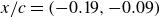
, respectively) are extracted. The premultiplied spectra of both original and IMFs of streamwise velocity fluctuations (
$^p$
, respectively) are extracted. The premultiplied spectra of both original and IMFs of streamwise velocity fluctuations (
 $\varPhi ^+_{uu}/\lambda ^+_x$
, where
$\varPhi ^+_{uu}/\lambda ^+_x$
, where
 $\lambda ^+_x$
is the inner-scaled streamwise wavelength) and wall-pressure fluctuations (
$\lambda ^+_x$
is the inner-scaled streamwise wavelength) and wall-pressure fluctuations (
 $\varPhi ^+_{pp}/\lambda ^+_x$
) are estimated at
$\varPhi ^+_{pp}/\lambda ^+_x$
) are estimated at
 $x/c = -0.15$
. The streamwise wavelength is converted from the frequency by considering the Taylor hypothesis (Gibeau & Ghaemi Reference Gibeau and Ghaemi2021; Baars, Dacome & Lee Reference Baars, Dacome and Lee2024), and scaled with inner viscous scales. The
$x/c = -0.15$
. The streamwise wavelength is converted from the frequency by considering the Taylor hypothesis (Gibeau & Ghaemi Reference Gibeau and Ghaemi2021; Baars, Dacome & Lee Reference Baars, Dacome and Lee2024), and scaled with inner viscous scales. The
 $\varPhi ^+_{uu}$
and
$\varPhi ^+_{uu}$
and
 $\varPhi ^+_{pp}$
values are scaled using
$\varPhi ^+_{pp}$
values are scaled using
 $u_\tau ^2$
and
$u_\tau ^2$
and
 $\rho ^2u_\tau ^4$
(where
$\rho ^2u_\tau ^4$
(where
 $\rho$
is the fluid density), following Ghaemi & Scarano (Reference Ghaemi and Scarano2013). The results are shown in figures 7, 8 and 9. The EMD-based scale decomposition was also performed at two higher Reynolds number conditions (
$\rho$
is the fluid density), following Ghaemi & Scarano (Reference Ghaemi and Scarano2013). The results are shown in figures 7, 8 and 9. The EMD-based scale decomposition was also performed at two higher Reynolds number conditions (
 ${\textit{Re}}_c=2.03\times 10^5$
and
${\textit{Re}}_c=2.03\times 10^5$
and
 $2.70\times 10^5$
) for comparison. The detailed results are provided in Appendix B.
$2.70\times 10^5$
) for comparison. The detailed results are provided in Appendix B.
Figure 7. Premultiplied spectra of streamwise velocity fluctuations (
 $\varPhi ^+_{uu}/\lambda ^+_x$
) at
$\varPhi ^+_{uu}/\lambda ^+_x$
) at
 $x/c=-0.15$
estimated using data measured by (a) planar PIV and (b) tomo-PIV, respectively. The spectral peaks are denoted by magenta circles.
$x/c=-0.15$
estimated using data measured by (a) planar PIV and (b) tomo-PIV, respectively. The spectral peaks are denoted by magenta circles.

Figure 8. The premultiplied spectra (
 $\varPhi ^+_{uu}/\lambda ^+_x$
) of decomposed (
$\varPhi ^+_{uu}/\lambda ^+_x$
) of decomposed (
 $a$
,
$a$
,
 $c$
,
$c$
,
 $e$
,
$e$
,
 $g$
,
$g$
,
 $i$
)
$i$
)
 $\text{IMF}^u_1$
–
$\text{IMF}^u_1$
–
 $\text{IMF}^u_5$
from planar PIV and (
$\text{IMF}^u_5$
from planar PIV and (
 $b$
,
$b$
,
 $d$
,
$d$
,
 $f$
,
$f$
,
 $h$
,
$h$
,
 $j$
)
$j$
)
 $\text{IMF}^u_2$
–
$\text{IMF}^u_2$
–
 $\text{IMF}^u_6$
from tomo-PIV at
$\text{IMF}^u_6$
from tomo-PIV at
 $x/c=-0.15$
. The spectral peaks are denoted by magenta circles.
$x/c=-0.15$
. The spectral peaks are denoted by magenta circles.

Figure 9. The premultiplied spectrum of original
 $p'$
and decomposed
$p'$
and decomposed
 $\text{IMF}^p$
s obtained from the transducer at
$\text{IMF}^p$
s obtained from the transducer at
 $x/c=-0.15$
, with the maxima denoted by squares.
$x/c=-0.15$
, with the maxima denoted by squares.
The inner-scaled premultiplied spectra of original streamwise velocity fluctuations from planar PIV and tomo-PIV (figure 7) exhibit similar patterns, with high-energy inner peaks
 $\lambda _x^+ = 740$
and 720, respectively, at
$\lambda _x^+ = 740$
and 720, respectively, at
 $y^+ \lt 20$
, which are attributed to the quasi-streamwise vortices and velocity streaks (Wang, Hu & Zheng Reference Wang, Hu and Zheng2021). The spectrum from tomo-PIV (figure 7
$y^+ \lt 20$
, which are attributed to the quasi-streamwise vortices and velocity streaks (Wang, Hu & Zheng Reference Wang, Hu and Zheng2021). The spectrum from tomo-PIV (figure 7
 $b$
) exhibits high-frequency noise at
$b$
) exhibits high-frequency noise at
 $\lambda _x^+ \lt 100$
(
$\lambda _x^+ \lt 100$
(
 $f \gt 1900$
Hz) (Wernet Reference Wernet2017). The former frequency range is considered irrelevant for the present analysis.
$f \gt 1900$
Hz) (Wernet Reference Wernet2017). The former frequency range is considered irrelevant for the present analysis.
After applying EMD, the IMF
 $^u$
with increasing scales are obtained. For the IMF
$^u$
with increasing scales are obtained. For the IMF
 $^u$
from planar PIV, the inner-scaled premultiplied spectra peak at
$^u$
from planar PIV, the inner-scaled premultiplied spectra peak at
 $\lambda ^+_{peak}=310$
, 630, 1170, 2350 and 5470, as shown in figures 8(
$\lambda ^+_{peak}=310$
, 630, 1170, 2350 and 5470, as shown in figures 8(
 $a$
), 8(
$a$
), 8(
 $c$
), 8(
$c$
), 8(
 $e$
), 8(
$e$
), 8(
 $g$
), and 8(
$g$
), and 8(
 $i$
). The high-energy range of the premultiplied spectrum moves closer to the wall as the order of IMF
$i$
). The high-energy range of the premultiplied spectrum moves closer to the wall as the order of IMF
 $^u$
increases. Due to the alternating distribution of positive and negative structures, the resultant length of an individual structure is half of
$^u$
increases. Due to the alternating distribution of positive and negative structures, the resultant length of an individual structure is half of
 $\lambda ^+_{peak}$
(Gibeau & Ghaemi Reference Gibeau and Ghaemi2021). The half-lengths of the first three IMF
$\lambda ^+_{peak}$
(Gibeau & Ghaemi Reference Gibeau and Ghaemi2021). The half-lengths of the first three IMF
 $^u$
are consistent with the sizes of hairpins, hairpin packets and velocity streaks observed in figure 6, respectively. For IMF
$^u$
are consistent with the sizes of hairpins, hairpin packets and velocity streaks observed in figure 6, respectively. For IMF
 $^u_4$
and IMF
$^u_4$
and IMF
 $^u_5$
, the half of
$^u_5$
, the half of
 $\lambda ^+_{peak}$
exceeds
$\lambda ^+_{peak}$
exceeds
 $5.4\delta$
, corresponding to the elongated near-wall streaks (Jiménez et al. Reference Jiménez, Del Álamo and Flores2004). The former structures are not dominant at the present low Reynolds number condition. For IMF
$5.4\delta$
, corresponding to the elongated near-wall streaks (Jiménez et al. Reference Jiménez, Del Álamo and Flores2004). The former structures are not dominant at the present low Reynolds number condition. For IMF
 $^u_1$
from tomo-PIV, the smallest wavelength
$^u_1$
from tomo-PIV, the smallest wavelength
 $40l$
corresponds to the measurement noise of tomo-PIV, which comes from the volume reconstruction from projected particle images obtained by a finite number of cameras (Lynch & Scarano Reference Lynch and Scarano2014). Consequently, its premultiplied spectrum is not presented. For higher-order modes, the spectra of IMF
$40l$
corresponds to the measurement noise of tomo-PIV, which comes from the volume reconstruction from projected particle images obtained by a finite number of cameras (Lynch & Scarano Reference Lynch and Scarano2014). Consequently, its premultiplied spectrum is not presented. For higher-order modes, the spectra of IMF
 $^u_2$
to IMF
$^u_2$
to IMF
 $^u_5$
(figures 8
b,d, f,h) and the peak wavelength from tomo-PIV exhibit good agreement with those of IMF
$^u_5$
(figures 8
b,d, f,h) and the peak wavelength from tomo-PIV exhibit good agreement with those of IMF
 $^u_1$
to IMF
$^u_1$
to IMF
 $^u_4$
from the planar PIV result. The IMFs of wall-normal velocity fluctuations exhibit characteristic wavelengths similar to those of the streamwise component (see table 3) and are not elaborated here.
$^u_4$
from the planar PIV result. The IMFs of wall-normal velocity fluctuations exhibit characteristic wavelengths similar to those of the streamwise component (see table 3) and are not elaborated here.
Table 3. Characteristic wavelengths of the original signal and IMFs for
 $u'$
,
$u'$
,
 $v'$
and
$v'$
and
 $p'$
determined at
$p'$
determined at
 $x/c=-0.15$
.
$x/c=-0.15$
.

For the wall-pressure fluctuations, the spectrum of the original signal peaks at
 $\lambda _{peak}^+= 280$
(figure 9, black line), which is smaller than the value for the streamwise velocity fluctuations. This observation aligns with findings reported by Baars et al. (Reference Baars, Dacome and Lee2024) and Hassanein et al. (Reference Hassanein, Modesti, Scarano and Baars2024) at
$\lambda _{peak}^+= 280$
(figure 9, black line), which is smaller than the value for the streamwise velocity fluctuations. This observation aligns with findings reported by Baars et al. (Reference Baars, Dacome and Lee2024) and Hassanein et al. (Reference Hassanein, Modesti, Scarano and Baars2024) at
 ${\textit{Re}}_{\tau }= 550{-}5200$
. The same trend is also evident for the
${\textit{Re}}_{\tau }= 550{-}5200$
. The same trend is also evident for the
 $\text{IMF}^p$
and
$\text{IMF}^p$
and
 $\text{IMF}^u$
with the same orders, as shown in table 3.
$\text{IMF}^u$
with the same orders, as shown in table 3.
The energy content (
 $k$
) of each IMF
$k$
) of each IMF
 $^u$
or IMF
$^u$
or IMF
 $^p$
is defined following Sun & Yan (Reference Sun and Yan2017) as
$^p$
is defined following Sun & Yan (Reference Sun and Yan2017) as
 \begin{equation} k=\frac {\int {(\text{IMF}_i})^2\,{\rm d}t}{\sum _{i=1}^N\int {(\text{IMF}_i})^2\,{\rm d}t+\int {r^2\,{\rm d}t}}. \end{equation}
The energy contents of the IMF
 $^p$
are estimated at
$^p$
are estimated at
 $x/c=-0.15$
. Those of the IMF
$x/c=-0.15$
. Those of the IMF
 $^u$
are estimated at selected wall-normal locations
$^u$
are estimated at selected wall-normal locations
 $y^+=25$
, 41, 72 and 134 above the former transducer measured by planar PIV. The results are shown in figure 10. For the IMF
$y^+=25$
, 41, 72 and 134 above the former transducer measured by planar PIV. The results are shown in figure 10. For the IMF
 $^u$
(figure 10
$^u$
(figure 10
 $a$
), IMF
$a$
), IMF
 $^u_2$
exhibits the highest energy level of over 30 %. Considering the wavelength, this indicates the energy dominance of hairpin packets. The first three IMF
$^u_2$
exhibits the highest energy level of over 30 %. Considering the wavelength, this indicates the energy dominance of hairpin packets. The first three IMF
 $^u$
occupy energy more than 78.4 % in total. The high-order IMF
$^u$
occupy energy more than 78.4 % in total. The high-order IMF
 $^u$
are considered insignificant in the present analysis. For the IMF
$^u$
are considered insignificant in the present analysis. For the IMF
 $^p$
(figure 10
$^p$
(figure 10
 $b$
), the IMF
$b$
), the IMF
 $^p_1$
and IMF
$^p_1$
and IMF
 $^p_2$
with smaller wavelengths show substantial energy contributions, accounting for 41.0 % and 34.3 % in the total. This is attributed to the intense burst–sweep events in the high-frequency component of wall-pressure fluctuations (Thomas & Bull Reference Thomas and Bull1983). The cumulative energy of the first four
$^p_2$
with smaller wavelengths show substantial energy contributions, accounting for 41.0 % and 34.3 % in the total. This is attributed to the intense burst–sweep events in the high-frequency component of wall-pressure fluctuations (Thomas & Bull Reference Thomas and Bull1983). The cumulative energy of the first four
 $\text{IMF}^p$
occupies 94.5 % in total, indicating their dominance.
$\text{IMF}^p$
occupies 94.5 % in total, indicating their dominance.

Figure 10. The energy content of each
 $\text{IMF}$
at
$\text{IMF}$
at
 $x/c = -0.15$
: (
$x/c = -0.15$
: (
 $a$
) streamwise velocity fluctuations from planar PIV at
$a$
) streamwise velocity fluctuations from planar PIV at
 $y^+=25$
, 41, 72 and 134; (
$y^+=25$
, 41, 72 and 134; (
 $b$
) wall-pressure fluctuations.
$b$
) wall-pressure fluctuations.
6. Scale-dependent pressure–velocity correlation
The correlation (
 $R_{p_mu_n}$
) between the streamwise velocity and wall-pressure fluctuations at different scales is estimated using
$R_{p_mu_n}$
) between the streamwise velocity and wall-pressure fluctuations at different scales is estimated using
 $\text{IMF}^p_m$
and
$\text{IMF}^p_m$
and
 $\text{IMF}^u_n$
at the streamwise location of the reference pressure transducer (
$\text{IMF}^u_n$
at the streamwise location of the reference pressure transducer (
 $x/c=-0.15$
):
$x/c=-0.15$
):
 \begin{equation} R_{p_mu_n} = \frac {1}{\rho u_\infty ^3} \left \langle \text{IMF}^p_m(t) \times\text{IMF}^u_n(y^+, t) \right \rangle. \end{equation}
Accounting for the wavelengths of coherent structures and the energy contributions of corresponding IMFs (see figure 10), the first five IMF
 $^p$
and IMF
$^p$
and IMF
 $^u$
(
$^u$
(
 $1\leqslant m, n \leqslant 5$
) are selected for estimating
$1\leqslant m, n \leqslant 5$
) are selected for estimating
 $R_{p_mu_n}$
. The
$R_{p_mu_n}$
. The
 $R_{p_mu_n}$
values at
$R_{p_mu_n}$
values at
 $y^+=25$
,
$y^+=25$
,
 $41$
,
$41$
,
 $72$
and
$72$
and
 $134$
estimated using planar PIV data are shown in figure 11. (Results for higher
$134$
estimated using planar PIV data are shown in figure 11. (Results for higher
 ${\textit{Re}}_c$
are available in Appendix C.) Significant correlations arise in the buffer layer (
${\textit{Re}}_c$
are available in Appendix C.) Significant correlations arise in the buffer layer (
 $y^+= 25$
) and log layer (
$y^+= 25$
) and log layer (
 $y^+=41$
and
$y^+=41$
and
 $72$
). This is consistent with the dominant wall-pressure source identified by Garcia-Sagrado & Hynes (Reference Garcia-Sagrado and Hynes2012) for the same aerofoil model. As shown in figures 11(a–c), significant correlations appear at both the diagonal and the off-diagonal condition when
$72$
). This is consistent with the dominant wall-pressure source identified by Garcia-Sagrado & Hynes (Reference Garcia-Sagrado and Hynes2012) for the same aerofoil model. As shown in figures 11(a–c), significant correlations appear at both the diagonal and the off-diagonal condition when
 $m = n+1$
. The latter exhibits higher
$m = n+1$
. The latter exhibits higher
 $R_{p_mu_n}$
. Since characteristic wavelengths of
$R_{p_mu_n}$
. Since characteristic wavelengths of
 $\text{IMF}^p_{n+1}$
and
$\text{IMF}^p_{n+1}$
and
 $\text{IMF}^u_n$
share the closest similarity (see table 3), it suggests that wall-pressure fluctuations originate from the turbulent structure with a similar scale (Gibeau & Ghaemi Reference Gibeau and Ghaemi2021). This suggests that wall-pressure fluctuations exhibit a linear superposition behaviour with the field coherent structures, analogous to the superposition effect between the inner and outer turbulent motions (Marusic et al. Reference Marusic, Mathis and Hutchins2010a
; Mathis, Hutchins & Marusic Reference Mathis, Hutchins and Marusic2011; Baars, Hutchins & Marusic Reference Baars, Hutchins and Marusic2016). Recent studies of Baars et al. (Reference Baars, Dacome and Lee2024) observed the significant linear frequency coherence between wall-pressure and streamwise velocity fluctuations in the frequency domain for TBL,
$\text{IMF}^u_n$
share the closest similarity (see table 3), it suggests that wall-pressure fluctuations originate from the turbulent structure with a similar scale (Gibeau & Ghaemi Reference Gibeau and Ghaemi2021). This suggests that wall-pressure fluctuations exhibit a linear superposition behaviour with the field coherent structures, analogous to the superposition effect between the inner and outer turbulent motions (Marusic et al. Reference Marusic, Mathis and Hutchins2010a
; Mathis, Hutchins & Marusic Reference Mathis, Hutchins and Marusic2011; Baars, Hutchins & Marusic Reference Baars, Hutchins and Marusic2016). Recent studies of Baars et al. (Reference Baars, Dacome and Lee2024) observed the significant linear frequency coherence between wall-pressure and streamwise velocity fluctuations in the frequency domain for TBL,
 ${\textit{Re}}_{\tau } = 550{-}5200$
, which also indicates such a superposition effect. Moving away from the wall,
${\textit{Re}}_{\tau } = 550{-}5200$
, which also indicates such a superposition effect. Moving away from the wall,
 $R_{p_mu_n}$
becomes moderate in the wake region (
$R_{p_mu_n}$
becomes moderate in the wake region (
 $y^+ = 134$
, figure 11
$y^+ = 134$
, figure 11
 $d$
), indicating weak correlation. The
$d$
), indicating weak correlation. The
 $R_{p_mu_n}$
vakue based on tomo-PIV measurement also exhibits significant correlation when IMF
$R_{p_mu_n}$
vakue based on tomo-PIV measurement also exhibits significant correlation when IMF
 $^u_n$
and IMF
$^u_n$
and IMF
 $^p_m$
share similar scales (
$^p_m$
share similar scales (
 $m=n$
due to the existence of noise-related IMF
$m=n$
due to the existence of noise-related IMF
 $^u_1$
as shown in table 3), which is not elaborated here for brevity.
$^u_1$
as shown in table 3), which is not elaborated here for brevity.

Figure 11. Correlations between IMFs of streamwise velocity from planar PIV and wall-pressure fluctuations (
 $R_{p_mu_n}$
): (a–d)
$R_{p_mu_n}$
): (a–d)
 $y^+=25$
, 41, 72 and 134, respectively.
$y^+=25$
, 41, 72 and 134, respectively.
To figure out the spatial distribution of the pressure sources at each strongly correlated wavelength (
 $m=n+1$
and
$m=n+1$
and
 $m = n$
for two- and three-dimensional velocity fields, respectively), the spatial–temporal correlations (
$m = n$
for two- and three-dimensional velocity fields, respectively), the spatial–temporal correlations (
 $p$
–
$p$
–
 $u$
,
$u$
,
 $p$
–
$p$
–
 $v$
and
$v$
and
 $p$
–
$p$
–
 $w$
) are estimated using the extracted IMFs of the corresponding orders following
$w$
) are estimated using the extracted IMFs of the corresponding orders following
 \begin{equation} \left . \begin{array}{ll} \displaystyle R^{2\text{-}D}_{p_{n+1}U_n}(x,y) = \frac {1}{\rho u_\infty ^3} \left \langle \text{IMF}^p_{n+1}(t) \times\text{IMF}^{U}_n(t,x,y) \right \rangle ,\\[10pt] \displaystyle R^{3\text{-}D}_{p_{n}U_n}(x,y,z) = \frac {1}{\rho u_\infty ^3} \left \langle \text{IMF}^p_{n}(t) \times\text{IMF}^{U}_n(t,x,y,z) \right \rangle , \end{array}\right \} \end{equation}
where
 $U$
denotes
$U$
denotes
 $u'$
,
$u'$
,
 $v'$
and
$v'$
and
 $w'$
. The superscripts
$w'$
. The superscripts
 $2\text{-}D$
and
$2\text{-}D$
and
 $3\text{-}D$
mean that the IMF
$3\text{-}D$
mean that the IMF
 $^U$
come from planar PIV and tomo-PIV measurement, respectively. Positive and negative
$^U$
come from planar PIV and tomo-PIV measurement, respectively. Positive and negative
 $\text{IMF}^p$
are considered separately in (6.2) to isolate the related turbulent structures. The resultant scale-dependent spatial–temporal
$\text{IMF}^p$
are considered separately in (6.2) to isolate the related turbulent structures. The resultant scale-dependent spatial–temporal
 $p$
–
$p$
–
 $u$
correlations are denoted as
$u$
correlations are denoted as
 $R^{2-D+}_{p_{n+1}U_n}$
,
$R^{2-D+}_{p_{n+1}U_n}$
,
 $R^{2-D-}_{p_{n+1}U_n}$
,
$R^{2-D-}_{p_{n+1}U_n}$
,
 $R^{3-D+}_{p_nU_n}$
and
$R^{3-D+}_{p_nU_n}$
and
 $R^{3-D-}_{p_nU_n}$
, where superscript
$R^{3-D-}_{p_nU_n}$
, where superscript
 $+$
and
$+$
and
 $-$
indicate the sign of IMF
$-$
indicate the sign of IMF
 $^p$
.
$^p$
.

Figure 12. Spatial distribution of
 $R^{2D}_{p_{n+1}u_n}$
: (
$R^{2D}_{p_{n+1}u_n}$
: (
 $a, d$
)
$a, d$
)
 $n = 1$
, (
$n = 1$
, (
 $b, e$
)
$b, e$
)
 $n = 2$
, (
$n = 2$
, (
 $c, f$
)
$c, f$
)
 $n = 3$
, for (a–c)
$n = 3$
, for (a–c)
 $R^{2D+}_{p_{n+1}u_n}$
, (d–f)
$R^{2D+}_{p_{n+1}u_n}$
, (d–f)
 $-R^{2D-}_{p_{n+1}u_n}$
. The vector fields of the
$-R^{2D-}_{p_{n+1}u_n}$
. The vector fields of the
 $p$
–
$p$
–
 $u$
and
$u$
and
 $p$
–
$p$
–
 $v$
correlations are superimposed. The magenta dashed line denotes the location of the reference transducer.
$v$
correlations are superimposed. The magenta dashed line denotes the location of the reference transducer.
The contours of the
 $p$
–
$p$
–
 $u$
correlation estimated from planar PIV data (
$u$
correlation estimated from planar PIV data (
 $R^{2D}_{p_{n+1}U_n}$
) are shown in figure 12. The vector field associate with
$R^{2D}_{p_{n+1}U_n}$
) are shown in figure 12. The vector field associate with
 $R^{2D}_{p_{n+1}U_n}$
is superimposed. The correlations of negative
$R^{2D}_{p_{n+1}U_n}$
is superimposed. The correlations of negative
 $\text{IMF}^p_{n+1}$
are multiplied by
$\text{IMF}^p_{n+1}$
are multiplied by
 $-1$
to represent the exact flow direction (Gibeau & Ghaemi Reference Gibeau and Ghaemi2021). Since the first four
$-1$
to represent the exact flow direction (Gibeau & Ghaemi Reference Gibeau and Ghaemi2021). Since the first four
 $\text{IMF}^p$
occupy the dominant energy (figure 10), only
$\text{IMF}^p$
occupy the dominant energy (figure 10), only
 $R^{2D}_{p_{2}u_{1}}$
,
$R^{2D}_{p_{2}u_{1}}$
,
 $R^{2D}_{p_{3}u_{2}}$
and
$R^{2D}_{p_{3}u_{2}}$
and
 $R^{2D}_{p_{4}u_{3}}$
are discussed. The correlation pattern for
$R^{2D}_{p_{4}u_{3}}$
are discussed. The correlation pattern for
 $R^{2D}_{p_{1}u_{1}}$
is similar to that for
$R^{2D}_{p_{1}u_{1}}$
is similar to that for
 $R^{2D}_{p_{2}u_{1}}$
with a smaller length scale. The former is not discussed here for conciseness.
$R^{2D}_{p_{2}u_{1}}$
with a smaller length scale. The former is not discussed here for conciseness.
For
 $R^{2D}_{p_{2}u_{1}}$
(figures 12
a,d), alternating positive and negative correlation regions with lengths approximately
$R^{2D}_{p_{2}u_{1}}$
(figures 12
a,d), alternating positive and negative correlation regions with lengths approximately
 $200 l$
and
$200 l$
and
 $100 l$
, respectively, arise around the reference transducer. The vector field indicates that the positive wall-pressure fluctuations (
$100 l$
, respectively, arise around the reference transducer. The vector field indicates that the positive wall-pressure fluctuations (
 $R^{2D+}_{p_{2}u_{1}}$
, figure 12
$R^{2D+}_{p_{2}u_{1}}$
, figure 12
 $a$
) occur when the upstream sweep and downstream ejection motions impinge, forming a stagnated shear layer, which is related to the turbulent motions induced between two adjacent hairpin-like vortices as observed in the three-dimensional instantaneous fields (figure 6
$a$
) occur when the upstream sweep and downstream ejection motions impinge, forming a stagnated shear layer, which is related to the turbulent motions induced between two adjacent hairpin-like vortices as observed in the three-dimensional instantaneous fields (figure 6
 $b$
4). The negative wall-pressure fluctuations (
$b$
4). The negative wall-pressure fluctuations (
 $-R^{2D-}_{p_{2}u_{1}}$
, figure 12
$-R^{2D-}_{p_{2}u_{1}}$
, figure 12
 $d$
) correspond to the fluid splitting due to upstream ejection and downstream sweep motions, which occur around the spanwise component of hairpins (figure 6
$d$
) correspond to the fluid splitting due to upstream ejection and downstream sweep motions, which occur around the spanwise component of hairpins (figure 6
 $b$
1) and canes (figure 6
$b$
1) and canes (figure 6
 $b$
2). This is consistent with the findings reported by Gibeau & Ghaemi (Reference Gibeau and Ghaemi2021), who demonstrated that the sweep and ejection motions induced by hairpins contribute to the mid-frequency wall-pressure fluctuations. The intermittent large-scale sweep and ejection motions also induce positive and negative curvatures of the velocity profiles (Ghaemi & Scarano Reference Ghaemi and Scarano2013), which lead to the increase of the mean shear and drive the rapid pressure term (Kraichnan Reference Kraichnan1956). For
$b$
2). This is consistent with the findings reported by Gibeau & Ghaemi (Reference Gibeau and Ghaemi2021), who demonstrated that the sweep and ejection motions induced by hairpins contribute to the mid-frequency wall-pressure fluctuations. The intermittent large-scale sweep and ejection motions also induce positive and negative curvatures of the velocity profiles (Ghaemi & Scarano Reference Ghaemi and Scarano2013), which lead to the increase of the mean shear and drive the rapid pressure term (Kraichnan Reference Kraichnan1956). For
 $R^{2D}_{p_{3}u_{2}}$
(figures 12
b,e), the alternating correlation regions extend in the streamwise direction, yielding a larger length, approximately
$R^{2D}_{p_{3}u_{2}}$
(figures 12
b,e), the alternating correlation regions extend in the streamwise direction, yielding a larger length, approximately
 $300l$
. The organisations of correlation patterns exhibit similarity with those of
$300l$
. The organisations of correlation patterns exhibit similarity with those of
 $R^{2D}_{p_{2}u_{1}}$
, indicating the self-similarity between these two structures (Marusic & Monty Reference Marusic and Monty2019; Baars & Marusic Reference Baars and Marusic2020; Gibeau & Ghaemi Reference Gibeau and Ghaemi2021). The pressure source corresponds to the uniform momentum zones (UMZs) enclosing multiple hairpin packets (Adrian, Meinhart & Tomkins Reference Adrian, Meinhart and Tomkins2000; Adrian Reference Adrian2007). For
$R^{2D}_{p_{2}u_{1}}$
, indicating the self-similarity between these two structures (Marusic & Monty Reference Marusic and Monty2019; Baars & Marusic Reference Baars and Marusic2020; Gibeau & Ghaemi Reference Gibeau and Ghaemi2021). The pressure source corresponds to the uniform momentum zones (UMZs) enclosing multiple hairpin packets (Adrian, Meinhart & Tomkins Reference Adrian, Meinhart and Tomkins2000; Adrian Reference Adrian2007). For
 $R^{2D}_{p_{4}u_{3}}$
, a single positively correlated region with length over
$R^{2D}_{p_{4}u_{3}}$
, a single positively correlated region with length over
 $500l$
is observed upstream of the reference transducer (figures 12
c,f). The corresponding height is reduced by 50 % compared with heights of
$500l$
is observed upstream of the reference transducer (figures 12
c,f). The corresponding height is reduced by 50 % compared with heights of
 $R^{2D}_{p_{2}u_{1}}$
and
$R^{2D}_{p_{2}u_{1}}$
and
 $R^{2D}_{p_{3}u_{2}}$
, with the wall-normal component weak. As a result, the positive and negative IMF
$R^{2D}_{p_{3}u_{2}}$
, with the wall-normal component weak. As a result, the positive and negative IMF
 $^p_4$
are related to the high- and low-speed velocity streaks (figure 6
$^p_4$
are related to the high- and low-speed velocity streaks (figure 6
 $a$
), being accompanied by weak sweep and ejection motions, respectively. The contribution of elongated velocity streaks to the low-frequency wall-pressure source is also reported by Pan & Ye (Reference Pan and Ye2025) close to the trailing edge of an NACA0018 aerofoil.
$a$
), being accompanied by weak sweep and ejection motions, respectively. The contribution of elongated velocity streaks to the low-frequency wall-pressure source is also reported by Pan & Ye (Reference Pan and Ye2025) close to the trailing edge of an NACA0018 aerofoil.

Figure 13. Spatial distribution of
 $R^{3D}_{p_{n}u_n}$
: (
$R^{3D}_{p_{n}u_n}$
: (
 $a$
,
$a$
,
 $d$
,
$d$
,
 $g$
,
$g$
,
 $j$
)
$j$
)
 $n =2$
, (
$n =2$
, (
 $b$
,
$b$
,
 $e$
,
$e$
,
 $h$
,
$h$
,
 $k$
)
$k$
)
 $n =3$
, (
$n =3$
, (
 $c$
,
$c$
,
 $f$
,
$f$
,
 $i$
,
$i$
,
 $l$
)
$l$
)
 $n =4$
. The three-dimensional distributions of (
$n =4$
. The three-dimensional distributions of (
 $a$
–
$a$
–
 $c$
)
$c$
)
 $R^{3D+}_{p_{n}u_n}$
and (
$R^{3D+}_{p_{n}u_n}$
and (
 $g$
–
$g$
–
 $i$
)
$i$
)
 $-R^{3D-}_{p_{n}u_n}$
are shown by red (positive value) and blue (negative value) iso-surface, respectively. Iso-values are set to
$-R^{3D-}_{p_{n}u_n}$
are shown by red (positive value) and blue (negative value) iso-surface, respectively. Iso-values are set to
 $|R^{3D}_{p_{n}u_n}|=3.5\times 10^{-6}$
,
$|R^{3D}_{p_{n}u_n}|=3.5\times 10^{-6}$
,
 $2.5\times 10^{-6}$
and
$2.5\times 10^{-6}$
and
 $1.5\times 10^{-6}$
for
$1.5\times 10^{-6}$
for
 $n=2,3,4$
, respectively. The cross-plane (
$n=2,3,4$
, respectively. The cross-plane (
 $x{-}z$
) contours of (d–f)
$x{-}z$
) contours of (d–f)
 $R^{3D+}_{p_{n}u_n}$
and (j–l)
$R^{3D+}_{p_{n}u_n}$
and (j–l)
 $-R^{3D-}_{p_{n}u_n}$
at
$-R^{3D-}_{p_{n}u_n}$
at
 $y^+=50$
are also shown, superimposed with vector fields of (
$y^+=50$
are also shown, superimposed with vector fields of (
 $p$
–
$p$
–
 $u$
,
$u$
,
 $p$
–
$p$
–
 $w$
) correlation. The reference transducer is denoted by the black circles.
$w$
) correlation. The reference transducer is denoted by the black circles.
Similarly, the three-dimensional spatial distributions of
 $p$
–
$p$
–
 $u$
correlations (
$u$
correlations (
 $R^{3D}_{p_{n}u_n}$
) are estimated based on the velocity fields obtained from tomo-PIV measurement, as shown in figure 13. The strongly correlated modes of
$R^{3D}_{p_{n}u_n}$
) are estimated based on the velocity fields obtained from tomo-PIV measurement, as shown in figure 13. The strongly correlated modes of
 $m = n$
(
$m = n$
(
 $n=2{-}4$
) are considered. The three-dimensional correlation of
$n=2{-}4$
) are considered. The three-dimensional correlation of
 $R^{3D}_{p_2u_2}$
(figures 13
a,g) and
$R^{3D}_{p_2u_2}$
(figures 13
a,g) and
 $R^{3D}_{p_3u_3}$
(figures 13
b,h) exhibit alternating positive and negative correlation regions arise around the transducer with self-similarity. In particular, correlation vectors in the
$R^{3D}_{p_3u_3}$
(figures 13
b,h) exhibit alternating positive and negative correlation regions arise around the transducer with self-similarity. In particular, correlation vectors in the
 $x{-}z$
cross-plane at
$x{-}z$
cross-plane at
 $y^+=50$
show that low-speed motions are flanked by a pair of counter-rotating wall normal vortices (magenta arrows) for
$y^+=50$
show that low-speed motions are flanked by a pair of counter-rotating wall normal vortices (magenta arrows) for
 $R^{3D}_{p_2u_2}$
(figures 13
d,j). This corresponds to the legs of hairpins (Adrian Reference Adrian2007; Gibeau & Ghaemi Reference Gibeau and Ghaemi2021), which further proves the contribution of hairpin-related vortices to IMF
$R^{3D}_{p_2u_2}$
(figures 13
d,j). This corresponds to the legs of hairpins (Adrian Reference Adrian2007; Gibeau & Ghaemi Reference Gibeau and Ghaemi2021), which further proves the contribution of hairpin-related vortices to IMF
 $^p_2$
. Although the streamwise scale of
$^p_2$
. Although the streamwise scale of
 $R^{3D}_{p_3u_3}$
is larger than that of
$R^{3D}_{p_3u_3}$
is larger than that of
 $R^{3D}_{p_2u_2}$
, their spanwise scales are similar. For
$R^{3D}_{p_2u_2}$
, their spanwise scales are similar. For
 $R^{3D}_{p_4u_4}$
(figures 13
c,f,i,l), the elongated correlation regions are observed to appear side by side in the spanwise direction from the three-dimensional perspective. This is consistent with the spanwise distribution of the velocity streaks (Jiménez et al. Reference Jiménez, Del Álamo and Flores2004).
$R^{3D}_{p_4u_4}$
(figures 13
c,f,i,l), the elongated correlation regions are observed to appear side by side in the spanwise direction from the three-dimensional perspective. This is consistent with the spanwise distribution of the velocity streaks (Jiménez et al. Reference Jiménez, Del Álamo and Flores2004).
7. Scale-dependent conditional average
To further investigate the spatial–temporal evolution of turbulent structures modulating wall-pressure fluctuations of certain scales, the conditional average of original
 $u'$
and
$u'$
and
 $v'$
is performed based on the occurrence of zero-crossing (ZC) events (Baars et al. Reference Baars, Talluru, Hutchins and Marusic2015) of
$v'$
is performed based on the occurrence of zero-crossing (ZC) events (Baars et al. Reference Baars, Talluru, Hutchins and Marusic2015) of
 $\text{IMF}^p_2$
to
$\text{IMF}^p_2$
to
 $\text{IMF}^p_4$
. Considering the larger sampling ensemble size and higher signal-to-noise ratio, the scale-dependent conditional average is performed based on the velocity fields measured by planar PIV. The ZC events represent the change between positive and negative wall-pressure fluctuations. The criterion to detect positive (ZC
$\text{IMF}^p_4$
. Considering the larger sampling ensemble size and higher signal-to-noise ratio, the scale-dependent conditional average is performed based on the velocity fields measured by planar PIV. The ZC events represent the change between positive and negative wall-pressure fluctuations. The criterion to detect positive (ZC
 $^+$
) and negative (ZC
$^+$
) and negative (ZC
 $^-$
) zero-crossing events are given by
$^-$
) zero-crossing events are given by
 \begin{equation} \left . \begin{array}{ll} \displaystyle \text{ZC}^+ \quad \text{if } p' = 0\quad \&\quad {\rm d}p'/{\rm d}t \gt 0,\\ \displaystyle \text{ZC}^- \quad \text{if } p' = 0\quad \&\quad {\rm d}p'/{\rm d}t \lt 0. \end{array}\right \} \end{equation}
An example of the detected events is shown in figure 14(a) for the time series of
 $\text{IMF}^p_2$
. The events ZC
$\text{IMF}^p_2$
. The events ZC
 $^+$
and ZC
$^+$
and ZC
 $^-$
are marked with red upward and blue downward triangles, respectively. The adjacent positive and negative pressure peaks (PP
$^-$
are marked with red upward and blue downward triangles, respectively. The adjacent positive and negative pressure peaks (PP
 $^+$
and PP
$^+$
and PP
 $^-$
, marked with red circles and blue squares) are also selected as criteria to represent local pressure extrema. The time series resembles a sinusoid signal. The PP
$^-$
, marked with red circles and blue squares) are also selected as criteria to represent local pressure extrema. The time series resembles a sinusoid signal. The PP
 $^+$
, ZC
$^+$
, ZC
 $^-$
, PP
$^-$
, PP
 $^-$
and ZC
$^-$
and ZC
 $^+$
events correspond to phases
$^+$
events correspond to phases
 $\pi /2$
,
$\pi /2$
,
 $\pi$
,
$\pi$
,
 $3\pi /2$
and
$3\pi /2$
and
 $2\pi$
, respectively. The contours of conditional averaged streamwise velocity fluctuations (
$2\pi$
, respectively. The contours of conditional averaged streamwise velocity fluctuations (
 $\overline {u'}/u_{\infty }$
) based on aforementioned events of
$\overline {u'}/u_{\infty }$
) based on aforementioned events of
 $\text{IMF}^p_2$
to
$\text{IMF}^p_2$
to
 $\text{IMF}^p_4$
are shown in figures 14(b–d). The corresponding vector fields are superimposed to visualise the turbulent motions.
$\text{IMF}^p_4$
are shown in figures 14(b–d). The corresponding vector fields are superimposed to visualise the turbulent motions.

Figure 14. (a) Example of the time series of
 $\text{IMF}^p_2$
(black line) and detected events of PP
$\text{IMF}^p_2$
(black line) and detected events of PP
 $^+$
(
$^+$
(
 $\circ$
), ZC
$\circ$
), ZC
 $^-$
(
$^-$
(
 $\triangledown$
), PP
$\triangledown$
), PP
 $^-$
(
$^-$
(
 $\square$
) and ZC
$\square$
) and ZC
 $^+$
(
$^+$
(
 $\triangle$
). (b–d) Contours of conditional averaged streamwise velocity fluctuations (
$\triangle$
). (b–d) Contours of conditional averaged streamwise velocity fluctuations (
 $\overline {u'}/u_{\infty }$
) based on the pressure events of
$\overline {u'}/u_{\infty }$
) based on the pressure events of
 $\text{IMF}^p_2$
,
$\text{IMF}^p_2$
,
 $\text{IMF}^p_3$
and
$\text{IMF}^p_3$
and
 $\text{IMF}^p_4$
. The vector fields are superimposed. Images 1–4 are based on the PP
$\text{IMF}^p_4$
. The vector fields are superimposed. Images 1–4 are based on the PP
 $^+$
, ZC
$^+$
, ZC
 $^-$
, PP
$^-$
, PP
 $^-$
, and ZC
$^-$
, and ZC
 $^+$
events, respectively. The magenta dashed line denotes the location of the reference transducer.
$^+$
events, respectively. The magenta dashed line denotes the location of the reference transducer.
For all the IMF
 $^p$
, the convection of the dominant high- and low-speed structures is observed, following the phase evolutions of wall-pressure fluctuations. For IMF
$^p$
, the convection of the dominant high- and low-speed structures is observed, following the phase evolutions of wall-pressure fluctuations. For IMF
 $^p_2$
(figure 14
b), a high-speed structure of length
$^p_2$
(figure 14
b), a high-speed structure of length
 $200l$
initially appears upstream of the reference transducer, being followed by a weaker low-speed structure for the PP
$200l$
initially appears upstream of the reference transducer, being followed by a weaker low-speed structure for the PP
 $^+$
event (phase
$^+$
event (phase
 $\pi /2$
, figure 14
b1). The former structures are associated with upstream sweep and downstream ejection motions, forming an impinging shear layer that induces a positive pressure peak. As the phase increases, the high-speed structure evolves downstream, locating directly above the transducer for phase
$\pi /2$
, figure 14
b1). The former structures are associated with upstream sweep and downstream ejection motions, forming an impinging shear layer that induces a positive pressure peak. As the phase increases, the high-speed structure evolves downstream, locating directly above the transducer for phase
 $\pi$
(ZC
$\pi$
(ZC
 $^-$
, figure 14
b2). The associated sweep motion becomes dominant, causing a positive-to-negative shift in wall-pressure fluctuations. At phase
$^-$
, figure 14
b2). The associated sweep motion becomes dominant, causing a positive-to-negative shift in wall-pressure fluctuations. At phase
 $3\pi/2$
(figure 14
b3), a weak low-speed motion forms upstream of the high-speed one. The fluid splitting due to upstream ejection and downstream sweep is produced above the transducer, triggering a negative pressure peak (PP
$3\pi/2$
(figure 14
b3), a weak low-speed motion forms upstream of the high-speed one. The fluid splitting due to upstream ejection and downstream sweep is produced above the transducer, triggering a negative pressure peak (PP
 $^-$
). For the final phase
$^-$
). For the final phase
 $2\pi$
(figure 14
b4), the low-speed motion further intensifies, locating directly above the reference transducer. The corresponding strong ejection motion leads to the ZC
$2\pi$
(figure 14
b4), the low-speed motion further intensifies, locating directly above the reference transducer. The corresponding strong ejection motion leads to the ZC
 $^+$
event (
$^+$
event (
 ${\rm d}p'/{\rm d}t \gt 0$
). One can find that the occurrence of pressure peaks and ZC events for IMF
${\rm d}p'/{\rm d}t \gt 0$
). One can find that the occurrence of pressure peaks and ZC events for IMF
 $^p_2$
is related to the convection of the hairpin-related vortices, highlighting the modulation on wall-pressure fluctuations by the vortical structures at different relative locations.
$^p_2$
is related to the convection of the hairpin-related vortices, highlighting the modulation on wall-pressure fluctuations by the vortical structures at different relative locations.
For higher-order modes of IMF
 $^p_3$
(figure 14
c), the phase evolution of turbulent structures with larger length approximately
$^p_3$
(figure 14
c), the phase evolution of turbulent structures with larger length approximately
 $300l$
remains similar to that of IMF
$300l$
remains similar to that of IMF
 $^p_2$
. The strength of low-speed structures increases to a level similar to the high-speed ones. The former structures correspond to the convection of high-speed regions at the spanwise side of the hairpin packets (
$^p_2$
. The strength of low-speed structures increases to a level similar to the high-speed ones. The former structures correspond to the convection of high-speed regions at the spanwise side of the hairpin packets (
 $u'\gt 0$
) and low-speed regions (
$u'\gt 0$
) and low-speed regions (
 $u'\lt 0$
) within packets, respectively (Ganapathisubramani, Longmire & Marusic Reference Ganapathisubramani, Longmire and Marusic2003; Marusic & Monty Reference Marusic and Monty2019; Baars & Marusic Reference Baars and Marusic2020). For
$u'\lt 0$
) within packets, respectively (Ganapathisubramani, Longmire & Marusic Reference Ganapathisubramani, Longmire and Marusic2003; Marusic & Monty Reference Marusic and Monty2019; Baars & Marusic Reference Baars and Marusic2020). For
 $\text{IMF}^p_4$
(figure 14
d), the structures turn to elongated streaks with larger length over
$\text{IMF}^p_4$
(figure 14
d), the structures turn to elongated streaks with larger length over
 $500l$
, exhibiting much weaker wall-normal motions. The turbulent structures responsible for the positive and negative pressure peaks change into the single upstream high- and low-speed motions, respectively (phases
$500l$
, exhibiting much weaker wall-normal motions. The turbulent structures responsible for the positive and negative pressure peaks change into the single upstream high- and low-speed motions, respectively (phases
 $\pi/2$
and
$\pi/2$
and
 $3\pi/2$
, figures 14
d1,d3). When the ZC events occur (phases
$3\pi/2$
, figures 14
d1,d3). When the ZC events occur (phases
 $\pi$
and
$\pi$
and
 $2\pi$
, figures 14
d2,d4), a pair of velocity streaks emerges. The sign change of velocity streaks agrees with that of the wall-pressure fluctuations.
$2\pi$
, figures 14
d2,d4), a pair of velocity streaks emerges. The sign change of velocity streaks agrees with that of the wall-pressure fluctuations.
8. Conclusion
In the present study, we investigated the scale-dependent links between turbulent structures and wall-pressure fluctuations in the TBL near the trailing edge of an NACA0012 aerofoil. Simultaneous wall-pressure and planar/tomographic PIV measurements were performed at
 ${\textit{Re}}_\tau=216$
to identify the wall-pressure sources. The wall-pressure and velocity fluctuations are decomposed using 1-D EMD into IMFs of increasing scales,
${\textit{Re}}_\tau=216$
to identify the wall-pressure sources. The wall-pressure and velocity fluctuations are decomposed using 1-D EMD into IMFs of increasing scales,
 $\lambda _x^{+}=130{-}6320$
. The characteristic wavelength of wall-pressure fluctuations is smaller than that of velocity for both original signal and decomposed IMFs with the same order. However, the scale-dependent spatial–temporal
$\lambda _x^{+}=130{-}6320$
. The characteristic wavelength of wall-pressure fluctuations is smaller than that of velocity for both original signal and decomposed IMFs with the same order. However, the scale-dependent spatial–temporal
 $p$
–
$p$
–
 $u$
correlation reveals that wall-pressure and velocity fluctuations exhibit the strongest correlation when they share a similar length scale. The patterns of the most correlated modes (
$u$
correlation reveals that wall-pressure and velocity fluctuations exhibit the strongest correlation when they share a similar length scale. The patterns of the most correlated modes (
 $R^{2D}_{p_{n+1}u_{n}}$
for
$R^{2D}_{p_{n+1}u_{n}}$
for
 $n= 1,3$
, and
$n= 1,3$
, and
 $R^{3D}_{p_{n}u_{n}}$
for
$R^{3D}_{p_{n}u_{n}}$
for
 $n=2,4$
) are identified, corresponding to the hairpins, UMZs of hairpin packets, and velocity streaks in the instantaneous flow.
$n=2,4$
) are identified, corresponding to the hairpins, UMZs of hairpin packets, and velocity streaks in the instantaneous flow.
The conditional average of
 $u'$
and
$u'$
and
 $v'$
based on detecting the PP and ZC events of
$v'$
based on detecting the PP and ZC events of
 $\text{IMF}^p_2$
to
$\text{IMF}^p_2$
to
 $\text{IMF}^p_4$
reveals how the turbulent structures evolve and modulate the wall-pressure fluctuations. Strong scale dependence is observed. For
$\text{IMF}^p_4$
reveals how the turbulent structures evolve and modulate the wall-pressure fluctuations. Strong scale dependence is observed. For
 $\text{IMF}^p_2$
and
$\text{IMF}^p_2$
and
 $\text{IMF}^p_3$
(related to hairpins and UMZs, respectively), the positive and negative pressure peaks are induced by fluid impinging and splitting, respectively, leading to the formation of the inclined shear layer. On the other hand, the ZC
$\text{IMF}^p_3$
(related to hairpins and UMZs, respectively), the positive and negative pressure peaks are induced by fluid impinging and splitting, respectively, leading to the formation of the inclined shear layer. On the other hand, the ZC
 $^+$
and ZC
$^+$
and ZC
 $^-$
events are related to the single high- and low-speed motions located directly on top of the pressure transducer, being accompanied by strong sweep and ejection motions, respectively. For
$^-$
events are related to the single high- and low-speed motions located directly on top of the pressure transducer, being accompanied by strong sweep and ejection motions, respectively. For
 $\text{IMF}^p_4$
of larger length scale, the upstream high- and low-speed streaks are responsible for the positive and negative pressure peaks, respectively. The transition between low- and high-speed velocity streaks coincides with the shift of negative/positive wall-pressure fluctuations. For all the
$\text{IMF}^p_4$
of larger length scale, the upstream high- and low-speed streaks are responsible for the positive and negative pressure peaks, respectively. The transition between low- and high-speed velocity streaks coincides with the shift of negative/positive wall-pressure fluctuations. For all the
 $\text{IMF}^p$
, the change from inducing a local inclined shear layer to single sweep/ejection events follows the temporal evolution of the turbulent motions, leading to the phase change of the wall-pressure signal.
$\text{IMF}^p$
, the change from inducing a local inclined shear layer to single sweep/ejection events follows the temporal evolution of the turbulent motions, leading to the phase change of the wall-pressure signal.
Supplementary movie
Supplementary movie is available at https://doi.org/10.1017/jfm.2026.11285.
Funding
This research has been supported by the National Natural Science Foundation of China (grant nos 12522213, 12372280) and the National Key R&D Program of China (grant no. 2020YFA0405700).
Declaration of interests
The authors report no conflict of interest.
Appendix A. Statistical convergence of planar PIV measurement
The premultiplied spectra of streamwise velocity fluctuations at
 $x/c=-0.15$
from planar PIV are estimated using 20 000, 50 000 and 100 000 snapshots (2 s, 5 s and 10 s, respectively), as shown in figure 15. For all the ensemble sizes, good agreement on the overall distribution and peak region is obtained. As a result, for the planar PIV measurement, good statistical convergence can be obtained with 20 000 snapshots (test duration 2 s).
$x/c=-0.15$
from planar PIV are estimated using 20 000, 50 000 and 100 000 snapshots (2 s, 5 s and 10 s, respectively), as shown in figure 15. For all the ensemble sizes, good agreement on the overall distribution and peak region is obtained. As a result, for the planar PIV measurement, good statistical convergence can be obtained with 20 000 snapshots (test duration 2 s).

Figure 15. The premultiplied spectra of streamwise velocity fluctuations calculated using three ensemble sizes of snapshots: (a) 20 000, (b) 50 000 and (c) 100 000 snapshots.
Appendix B. The EMD-based scale decomposition for higher Reynolds number
To investigate the Reynolds number effects, simultaneous
 $p$
–
$p$
–
 $u$
experiments of trailing-edge TBLs at higher Reynolds numbers were performed. Two additional free-stream velocities (
$u$
experiments of trailing-edge TBLs at higher Reynolds numbers were performed. Two additional free-stream velocities (
 $u_\infty$
) of 15 and 20 m s−1 are further tested using planar PIV and pressure transducers, corresponding to
$u_\infty$
) of 15 and 20 m s−1 are further tested using planar PIV and pressure transducers, corresponding to
 ${\textit{Re}}_c=2.03\times 10^5$
and
${\textit{Re}}_c=2.03\times 10^5$
and
 $2.70\times 10^5$
. The detailed boundary layer parameters at
$2.70\times 10^5$
. The detailed boundary layer parameters at
 $x/c = -0.15$
are provided in table 4.
$x/c = -0.15$
are provided in table 4.
Table 4. Summary of the boundary layer properties at
 $x/c=-0.15$
for
$x/c=-0.15$
for
 ${\textit{Re}}_c=2.03\times 10^5$
and
${\textit{Re}}_c=2.03\times 10^5$
and
 $2.70\times 10^5$
.
$2.70\times 10^5$
.
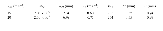
Using the EMD-based scale decomposition, the streamwise velocity and wall-pressure fluctuations are decomposed for higher Reynolds numbers (
 ${\textit{Re}}_c=2.03\times 10^5$
and
${\textit{Re}}_c=2.03\times 10^5$
and
 $2.70\times 10^5$
). The premultiplied spectra of IMF
$2.70\times 10^5$
). The premultiplied spectra of IMF
 $^u$
and IMF
$^u$
and IMF
 $^p$
are estimated, as shown in figures 16 and 17, respectively. The detailed characteristic wavelengths (
$^p$
are estimated, as shown in figures 16 and 17, respectively. The detailed characteristic wavelengths (
 $\lambda ^+_{peak}$
) determined through the spectral peaks are summarised in table 5. For the original data and decomposed IMFs, the peak wavelengths are observed to increase with the growth of the Reynolds number when compared with the results at
$\lambda ^+_{peak}$
) determined through the spectral peaks are summarised in table 5. For the original data and decomposed IMFs, the peak wavelengths are observed to increase with the growth of the Reynolds number when compared with the results at
 ${\textit{Re}}_c=1.35\times 10^5$
(table 3). This indicates the wavelength increase of corresponding turbulent structures as
${\textit{Re}}_c=1.35\times 10^5$
(table 3). This indicates the wavelength increase of corresponding turbulent structures as
 ${\textit{Re}}_c$
grows (Del Alamo et al. Reference Del Alamo, Jiménez, Zandonade and Moser2004).
${\textit{Re}}_c$
grows (Del Alamo et al. Reference Del Alamo, Jiménez, Zandonade and Moser2004).

Figure 16. The premultiplied spectra of IMF
 $^u$
at
$^u$
at
 $x/c=-0.15$
, for (a,c,e,g,i)
$x/c=-0.15$
, for (a,c,e,g,i)
 ${\textit{Re}}_c=2.03\times 10^5$
, (b,d,f,h,j)
${\textit{Re}}_c=2.03\times 10^5$
, (b,d,f,h,j)
 ${\textit{Re}}_c=2.70\times 10^5$
. The rows correspond to IMF
${\textit{Re}}_c=2.70\times 10^5$
. The rows correspond to IMF
 $^u$
of orders 1–5, respectively.
$^u$
of orders 1–5, respectively.
Table 5. Characteristic wavelengths of the original signal of
 $u'$
,
$u'$
,
 $p'$
and IMFs of different orders determined at
$p'$
and IMFs of different orders determined at
 $x/c=-0.15$
.
$x/c=-0.15$
.


Figure 17. The premultiplied spectra of wall-pressure fluctuations and corresponding IMF
 $^p$
at
$^p$
at
 $x/c=-0.15$
, for (a)
$x/c=-0.15$
, for (a)
 ${\textit{Re}}_c=2.03\times 10^5$
and (b)
${\textit{Re}}_c=2.03\times 10^5$
and (b)
 ${\textit{Re}}_c=2.70\times 10^5$
.
${\textit{Re}}_c=2.70\times 10^5$
.
The spectra of decomposed IMF
 $^u$
for
$^u$
for
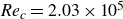 ${\textit{Re}}_c=2.03\times 10^5$
and
${\textit{Re}}_c=2.03\times 10^5$
and
 $2.70\times 10^5$
are presented in figure 16. The spectral distributions and scale increasing trend with the orders of IMFs are similar to those observed in the low Reynolds number case (figure 8). The wavelengths of
$2.70\times 10^5$
are presented in figure 16. The spectral distributions and scale increasing trend with the orders of IMFs are similar to those observed in the low Reynolds number case (figure 8). The wavelengths of
 $p'$
and IMF
$p'$
and IMF
 $^p$
are also observed to be smaller than those of
$^p$
are also observed to be smaller than those of
 $u'$
and IMF
$u'$
and IMF
 $^u$
of the same orders (Baars et al. Reference Baars, Dacome and Lee2024; Hassanein et al. Reference Hassanein, Modesti, Scarano and Baars2024).
$^u$
of the same orders (Baars et al. Reference Baars, Dacome and Lee2024; Hassanein et al. Reference Hassanein, Modesti, Scarano and Baars2024).
These results confirm the capability of EMD to separate overlapping scales of velocity and wall-pressure fluctuations in the aerofoil TBLs for all the flow conditions considered in the present study (Cheng et al. Reference Cheng, Li, Lozano-Durán and Liu2019; Mäteling & Schröder Reference Mäteling and Schröder2022).
Appendix C. Scale-dependent
$p$
–
$u$
correlation for higher Reynolds number


The
 $R_{p_mu_n}$
at higher Reynolds numbers (
$R_{p_mu_n}$
at higher Reynolds numbers (
 ${\textit{Re}}_c=2.03\times 10^5$
and
${\textit{Re}}_c=2.03\times 10^5$
and
 $2.70\times 10^5$
) are estimated using IMF
$2.70\times 10^5$
) are estimated using IMF
 $^u$
selected at buffer layer, log-layer, and wake regions. The results are shown in figure 18. The
$^u$
selected at buffer layer, log-layer, and wake regions. The results are shown in figure 18. The
 $R_{p_mu_n}$
at higher
$R_{p_mu_n}$
at higher
 ${\textit{Re}}_c$
exhibit the same trends as the significant correlations when IMF
${\textit{Re}}_c$
exhibit the same trends as the significant correlations when IMF
 $^u$
and IMF
$^u$
and IMF
 $^p$
share similar wavelengths (
$^p$
share similar wavelengths (
 $m=n+1$
). This suggests that the wall-pressure fluctuations exhibit a linear behaviour with the coherent structures, like the superposition effect between the inner and outer turbulence (Marusic et al. Reference Marusic, Mathis and Hutchins2010a
; Mathis et al. Reference Mathis, Hutchins and Marusic2011). The correlations also weaken as the IMF
$m=n+1$
). This suggests that the wall-pressure fluctuations exhibit a linear behaviour with the coherent structures, like the superposition effect between the inner and outer turbulence (Marusic et al. Reference Marusic, Mathis and Hutchins2010a
; Mathis et al. Reference Mathis, Hutchins and Marusic2011). The correlations also weaken as the IMF
 $^u$
move farther from the wall.
$^u$
move farther from the wall.
The spatial distributions of the strongly correlated
 $R_{p_mu_n}$
are also evaluated, with results shown in figure 19. For
$R_{p_mu_n}$
are also evaluated, with results shown in figure 19. For
 ${\textit{Re}}_c = 2.03\times 10^5$
and
${\textit{Re}}_c = 2.03\times 10^5$
and
 $2.70\times 10^5$
, the scale-dependent
$2.70\times 10^5$
, the scale-dependent
 $p$
–
$p$
–
 $u$
correlations exhibit distributions similar to those observed at
$u$
correlations exhibit distributions similar to those observed at
 ${\textit{Re}}_c = 1.35\times 10^5$
(figure 12). The correlation vectors and geometrical characteristics of the correlation regions for
${\textit{Re}}_c = 1.35\times 10^5$
(figure 12). The correlation vectors and geometrical characteristics of the correlation regions for
 $R_{p_2u_1}$
,
$R_{p_2u_1}$
,
 $R_{p_3u_2}$
and
$R_{p_3u_2}$
and
 $R_{p_4u_3}$
indicate that the corresponding wall-pressure sources are still hairpin, hairpin packet and velocity streaks, respectively. The inner-scaled length of
$R_{p_4u_3}$
indicate that the corresponding wall-pressure sources are still hairpin, hairpin packet and velocity streaks, respectively. The inner-scaled length of
 $p$
–
$p$
–
 $u$
correlation regions grows with increasing
$u$
correlation regions grows with increasing
 ${\textit{Re}}_c$
, indicating that the wall-pressure sources exhibit larger scales at higher Reynolds numbers.
${\textit{Re}}_c$
, indicating that the wall-pressure sources exhibit larger scales at higher Reynolds numbers.

Figure 18. Scale-dependent
 $p$
–
$p$
–
 $u$
correlation (
$u$
correlation (
 $R_{p_mu_n}$
) for higher
$R_{p_mu_n}$
) for higher
 ${\textit{Re}}_c$
at several wall-normal locations: (a–d)
${\textit{Re}}_c$
at several wall-normal locations: (a–d)
 ${\textit{Re}}_c=2.03\times 10^5$
, (e–h)
${\textit{Re}}_c=2.03\times 10^5$
, (e–h)
 ${\textit{Re}}_c=2.70\times 10^5$
.
${\textit{Re}}_c=2.70\times 10^5$
.
Figure 19. Spatial distribution of
 $R_{p_{n+1}u_n}$
of higher
$R_{p_{n+1}u_n}$
of higher
 ${\textit{Re}}_c$
: (a–f)
${\textit{Re}}_c$
: (a–f)
 ${\textit{Re}}_c = 2.03\times 10^5$
, (g–l)
${\textit{Re}}_c = 2.03\times 10^5$
, (g–l)
 ${\textit{Re}}_c = 2.70\times 10^5$
. Here, (a–c,g–i) correspond to
${\textit{Re}}_c = 2.70\times 10^5$
. Here, (a–c,g–i) correspond to
 $R^+_{p_2u_1}$
,
$R^+_{p_2u_1}$
,
 $R^+_{p_3u_2}$
and
$R^+_{p_3u_2}$
and
 $R^+_{p_4u_3}$
, and (d–f,j–l) correspond to
$R^+_{p_4u_3}$
, and (d–f,j–l) correspond to
 $-R^-_{p_2u_1}$
,
$-R^-_{p_2u_1}$
,
 $-R^-_{p_3u_2}$
and
$-R^-_{p_3u_2}$
and
 $-R^-_{p_4u_3}$
.
$-R^-_{p_4u_3}$
.


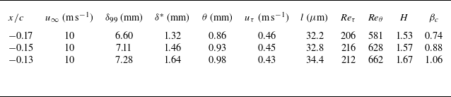


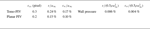


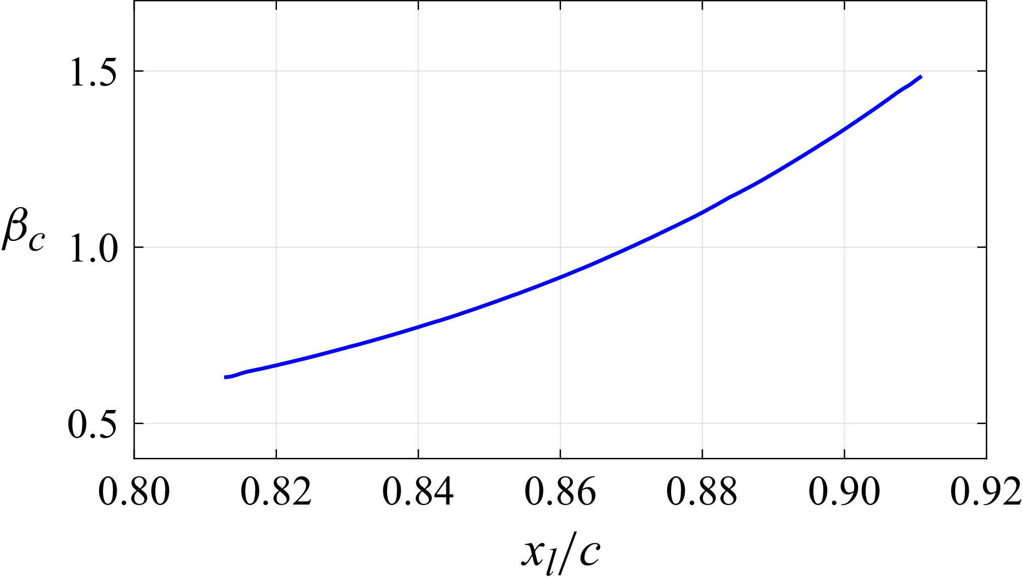

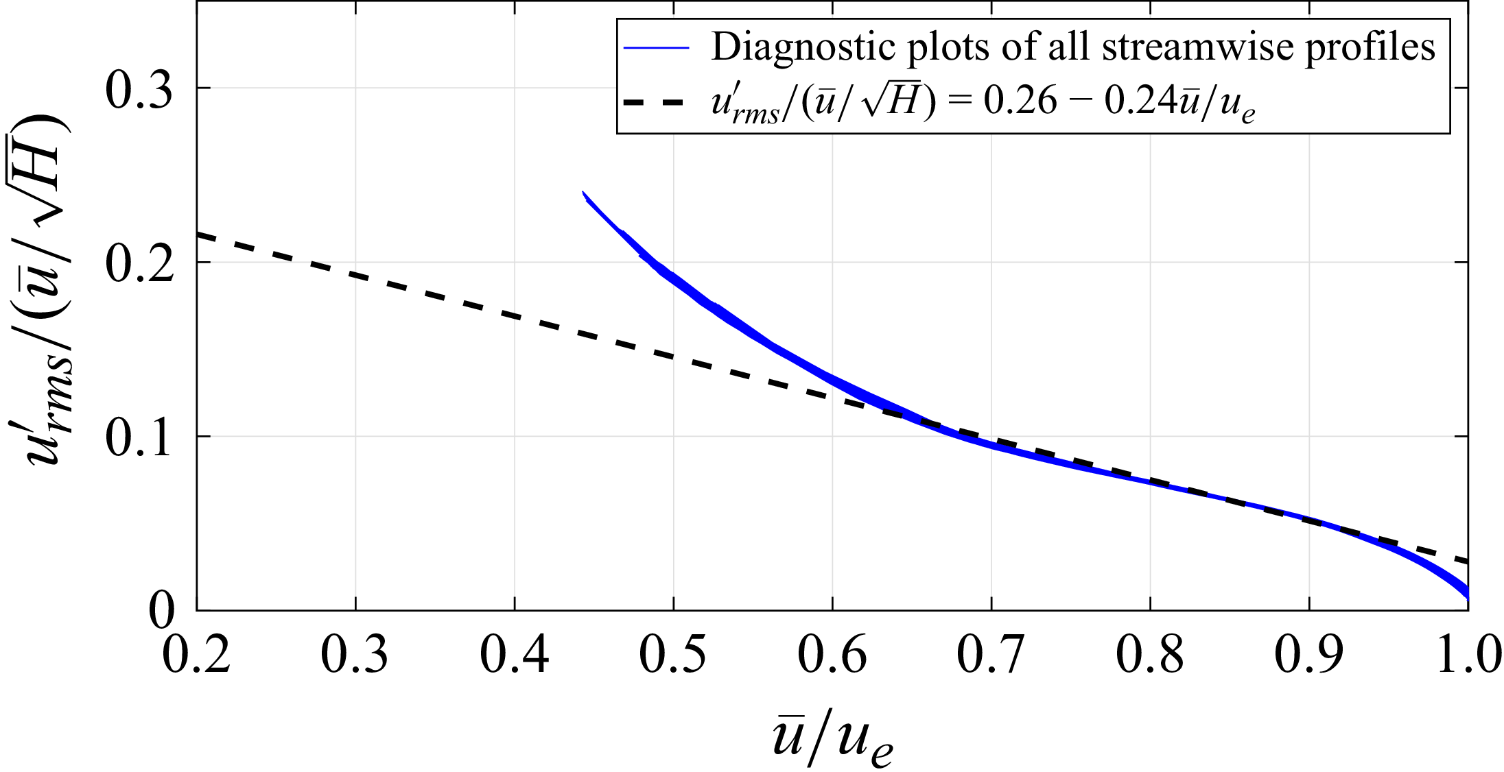

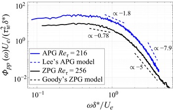
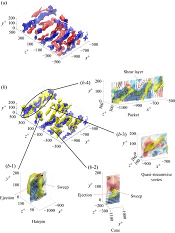


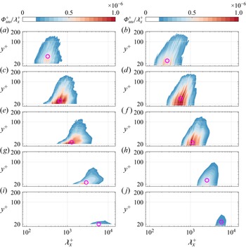


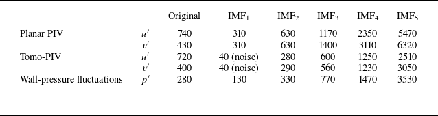


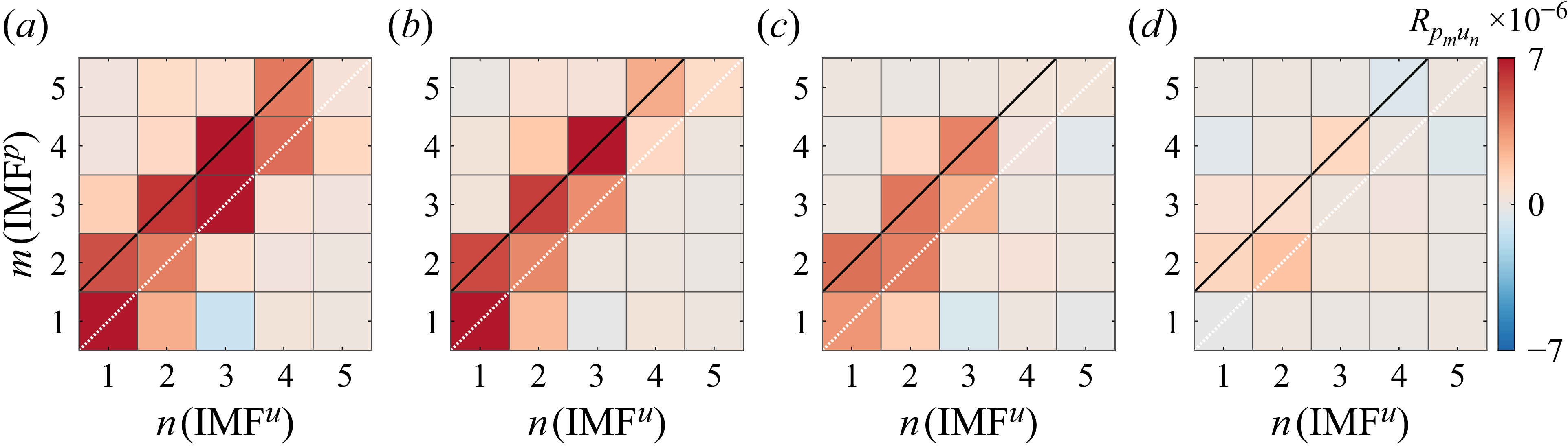


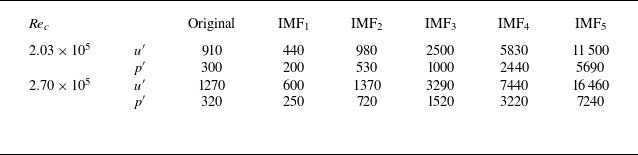


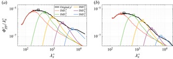


 Open access