





1. Introduction
Thin-film coatings are essential across numerous industrial applications, serving decorative, protective or functional roles. Achieving a uniform thickness distribution is often critical yet remains challenging even on simple geometries. On flat horizontal surfaces, the slightest topographical feature can deform the free surface over distances one to two orders of magnitude greater than the characteristic feature size – a classic example being comet tail defects in spin coating (Decré & Baret Reference Decré and Baret2003). Alternatively, controlled non-uniform patterns may be desired for microfabrication processes such as microarrays (McLeod, Liu & Troian Reference McLeod, Liu and Troian2011) or diffraction gratings (Brown et al. Reference Brown, Wells, Newton and McHale2009).
The mathematical modelling of thin liquid films often relies on the lubrication theory, which provides asymptotic simplifications of the Navier–Stokes equations in the thin-film limit. Comprehensive reviews of modelling and simulation approaches can be found in Craster & Matar (Reference Craster and Matar2009) and Kalliadasis et al. (Reference Kalliadasis, Ruyer-Quil, Scheid and Velarde2011), while Papageorgiou (Reference Papageorgiou2019) provides specialised coverage of electrically driven flows. For configurations where the film thickness is not small compared with the substrate curvature radius, reduced-order models extending beyond the lubrication limit have been developed for highly curved substrates (Wray, Papageorgiou & Matar Reference Wray, Papageorgiou and Matar2017; Wray & Cimpeanu Reference Wray and Cimpeanu2020; McKinlay, Wray & Wilson Reference McKinlay, Wray and Wilson2023). Various forcing mechanisms have been developed to achieve desired film-thickness distributions. The following key control strategies have received significant attention:
-
(i) Blowing/suction control: the application of blowing/suction to control the film-thickness distribution is a natural extension of Prandtl’s original idea to control boundary-layer separation on foils (Prandtl Reference Prandtl1927). Thompson, Tseluiko & Papageorgiou (Reference Thompson, Tseluiko and Papageorgiou2016b ) included the effects of blowing/suction in the long-wave thin-film approximation, and Thompson et al. (Reference Thompson, Gomes, Pavliotis and Papageorgiou2016a ) showed that the film-thickness distribution can be driven towards arbitrary steady states and travelling waves using blowing/suction. The approach was extended in Cimpeanu, Gomes & Papageorgiou (Reference Cimpeanu, Gomes and Papageorgiou2021) to control the complete nonlinear system governed by the Navier–Stokes equations using controls obtained from the lower-order, long-wave model.
-
(ii) Topographical control: the shape of the underlying substrate directly influences the free-surface shape and can therefore be used for control. In the lubrication approximation framework (low Reynolds number limit), Sellier (Reference Sellier2008) found an explicit expression predicting the required substrate shape for given plane flow conditions to generate a desired free-surface profile. This was extended to fully three-dimensional flows in Sellier & Panda (Reference Sellier and Panda2010a ). The substrate design problem was also considered in Binder, Blyth & McCue (Reference Binder, Blyth and McCue2013) and Robbins et al. (Reference Robbins, Blyth, Maclean and Binder2023) in the inviscid limit using a boundary integral approach for planar potential flows.
-
(iii) Marangoni flow control: because surface tension depends on temperature, controlling the free surface by imposing a local heat flux to prescribe the temperature distributions is a logical approach. Although thermocapillarity has been extensively studied since pioneering works by Tan, Bankoff & Davis (Reference Tan, Bankoff and Davis1990) and Burelbach, Bankoff & Davis (Reference Burelbach, Bankoff and Davis1990), the inverse problem of finding the required temperature distribution to deform the free surface in a desired way was first solved in Sellier & Panda (Reference Sellier and Panda2010b ) for plane flow and in Sellier & Panda (Reference Sellier and Panda2012) for three-dimensional flow in the long-wave approximation framework. Blyth & Bassom (Reference Blyth and Bassom2012) showed that the capillary ridge arising around substrate topographies could theoretically be removed by exploiting the thermocapillary effect. Likewise, Lunz (Reference Lunz2021) showed that free-surface deformations induced by pressure distributions could be eliminated using optimal temperature controls. The feasibility of this approach was convincingly demonstrated in Eshel et al. (Reference Eshel, Frumkin, Nice, Luria, Ferdman, Opatovski and Bercovici2022). Alternatively, surface tension can be altered by exposing photochemically active thin liquid films to light, a principle exploited in Kim et al. (Reference Kim, Janes, Zhou, Dulaney and Ellison2015) to control free-surface deformation using selective light exposure.
-
(iv) Electromagnetic control: when the free surface is subject to an electrical field, Maxwell stresses can be used to control free-surface deformation. The nonlinear dynamics of thin films subjected to mixed-frequency electrical fields was investigated in Duruk (Reference Duruk2020), demonstrating how frequency modulation can manipulate and control film behaviour. Wray, Cimpeanu & Gomes (Reference Wray, Cimpeanu and Gomes2022) showed, using optimal control of a reduced-order model, that applying a suitable potential at an electrode parallel to the substrate could control the interface shape. In magnetic wiping, Pino, Scheid & Mendez (Reference Pino, Scheid and Mendez2025) showed that the magnetic field distribution could be optimised to improve thin-film coating uniformity. Gabay et al. (Reference Gabay, Paratore, Boyko, Ramos, Gat and Bercovici2021) demonstrated in practice how the dielectrophoretic force could be used to shape thin liquid films.
-
(v) Kinematic control: using substrate motion and/or orientation to distribute the liquid film in a desired way has multiple consequences for the film-thickness distribution. The combination of external body forcing and surface geometry has been explored through high-frequency oscillation on cylindrical surfaces (Duruk & Oron Reference Duruk and Oron2014) and corrugated surfaces (Duruk & Oron Reference Duruk and Oron2016), shown to be effective for improving uniform or near-uniform coating profiles. Substrate orientation modifies the tangential and normal components of gravity, which was exploited in Boujo & Sellier (Reference Boujo and Sellier2019) to improve thin layer flow uniformity. Substrate motion also induces fictitious forces due to the non-inertial reference frame, which can be exploited to improve coating performance on curved substrates (Duruk et al. Reference Duruk, Boujo and Sellier2021, Reference Duruk, Shepherd, Boujo and Sellier2023; McIntyre et al. Reference McIntyre, Sellier, Gooch and Nock2024).
Most approaches in the thin-film control literature prescribe the geometry and/or forcing mechanisms a priori and analyse their effects on film behaviour. In all these approaches, the resulting film dynamics is analysed, optimised or stabilised with respect to a chosen objective. Recent optimal and feedback control strategies further extend this paradigm by dynamically adjusting actuation based on measured deviations from target states, typically through the minimisation of a cost functional (Thompson et al. Reference Thompson, Gomes, Pavliotis and Papageorgiou2016a ; Cimpeanu et al. Reference Cimpeanu, Gomes and Papageorgiou2021; Wray et al. Reference Wray, Cimpeanu and Gomes2022; Holroyd, Cimpeanu & Gomes Reference Holroyd, Cimpeanu and Gomes2025).
The present study takes a fundamentally different and complementary approach by addressing an inverse problem instead of an optimisation or feedback control task. Accordingly, this work does not formulate or solve a control problem: no objective functional is minimised, no robustness or optimality criteria are imposed and no feedback law is constructed. Forces or surface topography are not prescribed to study the ensuing film evolution, nor are deviations from a target state minimised. Instead, the desired outcome – uniform film thickness – is imposed directly as a steady solution of the governing lubrication model, and the corresponding body-force distributions required to admit and sustain this state are determined analytically.
The focus of this inverse formulation is on identifying forcing distributions compatible with the existence and stability of a uniform coating, rather than on optimality, robustness or dynamic feedback design. This methodology is motivated by previous investigations of the thin-film dynamics on rotating curved substrates (Duruk et al. Reference Duruk, Boujo and Sellier2021, Reference Duruk, Shepherd, Boujo and Sellier2023), which revealed fundamental limitations of intuitive forcing strategies. In particular, single-axis rotation at constant angular velocity was shown to be incapable of achieving a uniform coating on ellipsoidal geometries, highlighting the need for a systematic framework to determine the forcing distributions theoretically required to generate uniform coatings on arbitrary curved surfaces.
The novelty of this work lies in formulating and solving the inverse thin-film problem: for a prescribed uniform coating on an arbitrary curved substrate, we determine the body force required to achieve and stabilise it.
The remainder of this paper is organised as follows. Section 2 presents the mathematical model governing the thin-film dynamics on curved substrates subjected to arbitrary body forces. Section 3 derives the criterion for uniform coating by imposing a constant-thickness solution to determine the tangential forcing required for the existence of a uniform state, while the associated linear stability analysis establishes the constraints on the normal forcing components necessary to ensure coating stability. The methodology is demonstrated on constant-curvature geometries (flat plates and cylinders) and extended to surfaces with non-constant curvature (spheroids). Section 4 presents numerical experiments validating the theoretical predictions for spheroidal caps in both convex and concave configurations. Section 5 demonstrates a possible physical realisation of the required force distributions through multi-axial substrate rotation on a sphere. Concluding remarks are provided in § 6.
Schematic illustration of a thin liquid film of thickness $H$
coating a curved substrate
$H$
coating a curved substrate $\boldsymbol S$
, with outward unit normal
$\boldsymbol S$
, with outward unit normal $\boldsymbol n$
and body force
$\boldsymbol n$
and body force $\boldsymbol F$
.
$\boldsymbol F$
.

2. Mathematical model
We consider a thin liquid film deposited on the outer surface of a solid substrate. The film has a characteristic thickness $h_0$
, while the substrate is characterised by a length scale
$h_0$
, while the substrate is characterised by a length scale $R$
. The liquid is assumed to be incompressible, isothermal and Newtonian, with density
$R$
. The liquid is assumed to be incompressible, isothermal and Newtonian, with density $\rho$
, viscosity
$\rho$
, viscosity $\mu$
and surface tension
$\mu$
and surface tension $\sigma$
, while the surrounding gas phase is taken to be hydrodynamically passive, with negligible density and viscosity.
$\sigma$
, while the surrounding gas phase is taken to be hydrodynamically passive, with negligible density and viscosity.
The substrate surface is parametrised by $\boldsymbol{X} = (X_1, X_2)$
and described by the smooth mapping
$\boldsymbol{X} = (X_1, X_2)$
and described by the smooth mapping $\boldsymbol{S}(\boldsymbol{X})$
with unit outward normal
$\boldsymbol{S}(\boldsymbol{X})$
with unit outward normal $\boldsymbol{n}$
. The free surface
$\boldsymbol{n}$
. The free surface $\boldsymbol{S}_{\!f}$
is then given by
$\boldsymbol{S}_{\!f}$
is then given by
 \begin{equation} \boldsymbol{S}_{\!f}(\boldsymbol{X}, T) = \boldsymbol{S}(\boldsymbol{X}) + H(\boldsymbol{X}, T)\boldsymbol{n}, \end{equation}
where $H(\boldsymbol{X},T)\ge 0$
denotes the film thickness measured along the outward unit normal direction, and
$H(\boldsymbol{X},T)\ge 0$
denotes the film thickness measured along the outward unit normal direction, and $T$
denotes time.
$T$
denotes time.
The system is subjected to a body-force field $\boldsymbol F=(F_1,F_2,F_3)$
in Cartesian coordinates. Throughout this work, the forcing field
$\boldsymbol F=(F_1,F_2,F_3)$
in Cartesian coordinates. Throughout this work, the forcing field $\boldsymbol F$
represents any physically admissible body force, including gravitational effects and forces achievable through external actuation mechanisms. Physically admissible forces are assumed to be spatially smooth and bounded, consistent with the actuation mechanism employed; no further restriction is placed on the spatial dependence of
$\boldsymbol F$
represents any physically admissible body force, including gravitational effects and forces achievable through external actuation mechanisms. Physically admissible forces are assumed to be spatially smooth and bounded, consistent with the actuation mechanism employed; no further restriction is placed on the spatial dependence of $\boldsymbol{F}$
beyond these requirements. A schematic illustration of the geometry, shown here for a lens-like substrate, is provided in figure 1.
$\boldsymbol{F}$
beyond these requirements. A schematic illustration of the geometry, shown here for a lens-like substrate, is provided in figure 1.
The dimensionless lubrication model governing the evolution of the film thickness $h(\boldsymbol x,t)$
is derived under the standard long-wave limit: small aspect ratio (
$h(\boldsymbol x,t)$
is derived under the standard long-wave limit: small aspect ratio ( $\epsilon = h_0/R \ll 1$
) and negligible inertia (low Reynolds number). The body force
$\epsilon = h_0/R \ll 1$
) and negligible inertia (low Reynolds number). The body force $\boldsymbol F$
is taken to be steady or to vary on time scales of
$\boldsymbol F$
is taken to be steady or to vary on time scales of $O(\epsilon ^2)$
or slower, so as to remain consistent with the lubrication approximation. The film thickness and spatial coordinates are non-dimensionalised using
$O(\epsilon ^2)$
or slower, so as to remain consistent with the lubrication approximation. The film thickness and spatial coordinates are non-dimensionalised using $h_0$
and
$h_0$
and $R$
, respectively, while time is scaled by the viscocapillary time scale
$R$
, respectively, while time is scaled by the viscocapillary time scale $t_c = 3\mu R^4/(\sigma h_0^3)$
.
$t_c = 3\mu R^4/(\sigma h_0^3)$
.
Following the formulation developed in Thiffeault & Kamhawi (Reference Thiffeault and Kamhawi2006) and Duruk et al. (Reference Duruk, Shepherd, Boujo and Sellier2023), the governing equations are given by
 \begin{equation} n_h h_t + \boldsymbol{\nabla }\boldsymbol{\cdot }\left (\boldsymbol q_1 + \boldsymbol q_2\right ) = 0, \end{equation}
 \begin{equation} n_h = 1 - \epsilon \kappa h + \epsilon ^2 \mathcal{G} h^2, \end{equation}
 \begin{align} \boldsymbol q_1 = h^3 \left [\boldsymbol{\nabla }\tilde {\kappa } - h \left (\kappa I - \frac {1}{2}K\right )\boldsymbol{\nabla }\kappa \right ]\!, \quad \boldsymbol q_2 = h^3 \left [ \epsilon ^{-1} \boldsymbol f_{\!d} - h \left (\kappa I + \frac {1}{2}K\right )\boldsymbol f_{\!d} + f_3 \boldsymbol{\nabla }h \right ]\!, \\[-28pt] \nonumber \end{align}
 \begin{equation} \tilde {\kappa } = \boldsymbol{\nabla} ^2 h + \kappa _s h + \epsilon ^{-1}\kappa . \end{equation}
Equation (2.2) expresses conservation of mass and momentum for the liquid film. The depth-integrated flux $\boldsymbol q_1$
accounts for capillary-driven transport arising from gradients of the free-surface curvature, including corrections due to the substrate geometry. The flux
$\boldsymbol q_1$
accounts for capillary-driven transport arising from gradients of the free-surface curvature, including corrections due to the substrate geometry. The flux $\boldsymbol{q}_2$
represents transport induced by body forces, decomposed into tangential components
$\boldsymbol{q}_2$
represents transport induced by body forces, decomposed into tangential components $\boldsymbol{f}_{\!d} = (f_1, f_2)$
that drive direct surface flow, and a normal component
$\boldsymbol{f}_{\!d} = (f_1, f_2)$
that drive direct surface flow, and a normal component $f_3$
that couples to thickness gradients. The geometric quantities in (2.2) characterise the substrate surface through the curvature tensor
$f_3$
that couples to thickness gradients. The geometric quantities in (2.2) characterise the substrate surface through the curvature tensor $K$
and its associated scalar invariants: the mean curvature
$K$
and its associated scalar invariants: the mean curvature $\kappa = \textit{Tr}(K)$
, the Gaussian curvature
$\kappa = \textit{Tr}(K)$
, the Gaussian curvature $G = \det (K)$
and the squared curvature
$G = \det (K)$
and the squared curvature $\kappa _s = K^j_i K^i_{\!j}$
(with indices
$\kappa _s = K^j_i K^i_{\!j}$
(with indices $i, j = 1, 2$
). The quantity
$i, j = 1, 2$
). The quantity $\tilde {\kappa }$
represents the free-surface curvature approximation, while
$\tilde {\kappa }$
represents the free-surface curvature approximation, while $I$
denotes the identity tensor. No assumption of orthogonality or special coordinate structure is made in the surface parametrisation. All geometric operators are written in fully covariant/contravariant form and therefore remain valid for arbitrary smooth parametrisations of any substrate. Detailed definitions of the differential operators and tensors are provided in Appendix A.
$I$
denotes the identity tensor. No assumption of orthogonality or special coordinate structure is made in the surface parametrisation. All geometric operators are written in fully covariant/contravariant form and therefore remain valid for arbitrary smooth parametrisations of any substrate. Detailed definitions of the differential operators and tensors are provided in Appendix A.
It should be noted that the $O(\epsilon ^{-1})$
terms in (2.2) arise from a distinguished limit in which the substrate curvature radius is
$O(\epsilon ^{-1})$
terms in (2.2) arise from a distinguished limit in which the substrate curvature radius is $O(R)$
and the film thickness is
$O(R)$
and the film thickness is $O(\epsilon R)$
. In this regime, the substrate curvature
$O(\epsilon R)$
. In this regime, the substrate curvature $\kappa \sim O(1/R)$
enters the leading-order free-surface curvature as
$\kappa \sim O(1/R)$
enters the leading-order free-surface curvature as $\epsilon ^{-1}\kappa$
, ensuring that substrate geometry and film-thickness variations both influence the dynamics at the same asymptotic order. Alternative scalings that eliminate
$\epsilon ^{-1}\kappa$
, ensuring that substrate geometry and film-thickness variations both influence the dynamics at the same asymptotic order. Alternative scalings that eliminate $\epsilon ^{-1}$
terms are possible but would modify the normalisation of the equation.
$\epsilon ^{-1}$
terms are possible but would modify the normalisation of the equation.
This framework for curved substrates has been extensively developed (Roy, Roberts & Simpson Reference Roy, Roberts and Simpson2002; Thiffeault & Kamhawi Reference Thiffeault and Kamhawi2006) and validated against both full Navier–Stokes simulations (Duruk, Boujo & Sellier Reference Duruk, Boujo and Sellier2021; Ledda et al. Reference Ledda, Pezzulla, Jambon-Puillet, Brun and Gallaire2022) and experiments (Ledda et al. Reference Ledda, Pezzulla, Jambon-Puillet, Brun and Gallaire2022), demonstrating excellent quantitative agreement in the lubrication regime.
In the forward formulations, the body force and/or substrate geometry are prescribed and (2.2) is solved to predict film evolution. In the present work, we instead address the inverse problem: a desired uniform film thickness is imposed as a solution to (2.2), and the body-force distribution required to admit and sustain this state is systematically determined. This inverse perspective allows direct identification of forcing strategies compatible with uniform coating, rather than trial-and-error optimisation of prescribed forcings.
The following section is devoted to developing this inverse criterion and establishing the associated methodology. For clarity, table 1 summarises the key notations used for the body-force formulation throughout this work.
Summary of notation used throughout the manuscript for body-force formulation.

3. Criterion for uniform coating
In this section, we adopt an inverse-design approach to derive the conditions under which a uniform coating can be sustained on an arbitrary substrate. This inverse approach allows us to identify the tangential forcing required for the existence of a uniform coating, while the role of the normal forcing component emerges through the stability of this state.
For the uniform state, $h=1$
implies
$h=1$
implies $\boldsymbol{\nabla }h=\boldsymbol{0}$
and
$\boldsymbol{\nabla }h=\boldsymbol{0}$
and $\partial _t h=0$
. Substituting these conditions into the mass conservation (2.2) yields
$\partial _t h=0$
. Substituting these conditions into the mass conservation (2.2) yields
 \begin{equation} \boldsymbol{\nabla }\boldsymbol{\cdot }(\boldsymbol{q}_1 + \boldsymbol{q}_2) = 0. \end{equation}
The zero-divergence condition (3.1) requires that the total flux field $\boldsymbol{q}_1+\boldsymbol{q}_2$
be divergence free. While a divergence-free vector field need not vanish everywhere, the geometric and topological constraints of our configuration preclude non-zero constant flux solutions. For finite substrate patches with zero-flux boundary conditions
$\boldsymbol{q}_1+\boldsymbol{q}_2$
be divergence free. While a divergence-free vector field need not vanish everywhere, the geometric and topological constraints of our configuration preclude non-zero constant flux solutions. For finite substrate patches with zero-flux boundary conditions $\boldsymbol{q}\boldsymbol{\cdot }\boldsymbol{n}_{\partial D} = 0$
, any spatially constant tangential flux
$\boldsymbol{q}\boldsymbol{\cdot }\boldsymbol{n}_{\partial D} = 0$
, any spatially constant tangential flux $\boldsymbol{q} = \boldsymbol{c}$
would violate the boundary condition, since the outward normal
$\boldsymbol{q} = \boldsymbol{c}$
would violate the boundary condition, since the outward normal $\boldsymbol{n}_{\partial D}$
varies along the perimeter, making
$\boldsymbol{n}_{\partial D}$
varies along the perimeter, making $\boldsymbol{c}\boldsymbol{\cdot }\boldsymbol{n}_{\partial D} \neq 0$
at generic boundary points. For closed surfaces such as spheres and spheroids, a topological obstruction – the Poincaré–Hopf theorem (commonly known as the hairy ball theorem) – prevents the existence of a nowhere-vanishing smooth tangent vector field (in contrast to toroidal surfaces, where such fields are admissible). In physical terms, this reflects the impossibility of defining a smooth, non-vanishing tangential forcing field everywhere on a closed surface without introducing singular points. Consequently, the only admissible solution is
$\boldsymbol{c}\boldsymbol{\cdot }\boldsymbol{n}_{\partial D} \neq 0$
at generic boundary points. For closed surfaces such as spheres and spheroids, a topological obstruction – the Poincaré–Hopf theorem (commonly known as the hairy ball theorem) – prevents the existence of a nowhere-vanishing smooth tangent vector field (in contrast to toroidal surfaces, where such fields are admissible). In physical terms, this reflects the impossibility of defining a smooth, non-vanishing tangential forcing field everywhere on a closed surface without introducing singular points. Consequently, the only admissible solution is $\boldsymbol{q}_1 + \boldsymbol{q}_2 = \boldsymbol{0}$
, requiring the body-force-driven flux to exactly balance the capillary-driven flux at every point to achieve a quiescent film. We impose this pointwise balance condition to determine the uniform-coating forcing throughout this study.
$\boldsymbol{q}_1 + \boldsymbol{q}_2 = \boldsymbol{0}$
, requiring the body-force-driven flux to exactly balance the capillary-driven flux at every point to achieve a quiescent film. We impose this pointwise balance condition to determine the uniform-coating forcing throughout this study.
Evaluating the flux expressions at $h=1$
and imposing this balance condition, we obtain the following requirement on the tangential forcing:
$h=1$
and imposing this balance condition, we obtain the following requirement on the tangential forcing:
 \begin{equation} \boldsymbol{f}_{\!d} = \boldsymbol{f}_{\!0} = M_1 \boldsymbol{\nabla }\kappa _s + M_2 \boldsymbol{\nabla }\kappa , \end{equation}
where the matrices $M_1$
and
$M_1$
and $M_2$
are defined as
$M_2$
are defined as
 \begin{equation} M_1 = -A_2^{-1}, \quad M_2 = -A_2^{-1}(\epsilon ^{-1}I + A_1), \end{equation}
 \begin{equation} A_1 = -\left (\kappa I - \frac {1}{2}K\right )\!, \quad A_2 = \epsilon ^{-1}I - \left (\kappa I + \frac {1}{2}K\right )\!. \end{equation}
Equation (3.2) uniquely determines the tangential body force consistent with the lubrication approximation and constitutive assumptions required to sustain a uniform film thickness. We refer to $\boldsymbol{f}_{\!0}$
as the uniform-coating forcing. For fixed liquid properties, this forcing depends exclusively on the substrate geometry and may be used to either prescribe a forcing strategy that produces a homogeneous coating or to assess whether a given forcing configuration is capable of maintaining uniformity.
$\boldsymbol{f}_{\!0}$
as the uniform-coating forcing. For fixed liquid properties, this forcing depends exclusively on the substrate geometry and may be used to either prescribe a forcing strategy that produces a homogeneous coating or to assess whether a given forcing configuration is capable of maintaining uniformity.
3.1. Theoretical considerations
Before applying the uniform-coating forcing framework to specific geometries, we establish several general theoretical observations that clarify its structure and implications.
-
(i) Substrates of constant curvature. For substrates of constant curvature, including flat surfaces, circular cylinders and spheres, the gradients of both $\kappa$
and
$\kappa _s$
vanish identically. Equation (3.2) then immediately yields
$\boldsymbol{f}_{\!0} = 0$
, establishing that no non-trivial tangential forcing is admissible if a uniform coating is to be sustained on such geometries.
$\kappa$
and
$\kappa _s$
vanish identically. Equation (3.2) then immediately yields
$\boldsymbol{f}_{\!0} = 0$
, establishing that no non-trivial tangential forcing is admissible if a uniform coating is to be sustained on such geometries. -
(ii) Substrates of non-constant curvature. In contrast to the constant-curvature case, substrates with spatially varying curvature require non-trivial tangential forcing to maintain uniformity. For an arbitrary surface parametrisation, the explicit form of the uniform-coating forcing involves the full curvature tensor and the metric coefficients and is therefore geometrically intricate, but still computable. However, when the surface is parametrised using orthogonal coordinates, for which the metric tensor is diagonal, (3.2) simplifies considerably. Introducing the metric coefficients
$m_1,m_2$
and the principal curvatures
$k_1,k_2$
yields the closed-form expression(3.3)where
\begin{equation} f_0^i = \frac {(2 + \epsilon (4k_i - k_{\!j}))\partial _i k_i + (2 + 3\epsilon k_{\!j})\partial _i k_{\!j}} {m_i[\epsilon (3k_i + 2k_{\!j}) - 2]}, \quad i,j=1,2, \quad i \neq j, \end{equation}
$f_0^i$
denotes the tangential component of the uniform-coating forcing along the
$i$
th principal direction.


3.1.1. Role of the normal component
The normal component of the forcing plays a central and distinct role in the uniform-coating problem, governing the stability rather than the existence of the uniform state. Having determined the tangential forcing components that admit a uniform thickness solution, we now examine how the normal component governs the stability of this state through analysis of small perturbations.
The uniform-coating forcing $\boldsymbol f_0$
is a three-dimensional vector composed of two tangential components and one normal component relative to the substrate surface. The zero-divergence condition (3.1) provides only two independent equations and therefore determines only the tangential components
$\boldsymbol f_0$
is a three-dimensional vector composed of two tangential components and one normal component relative to the substrate surface. The zero-divergence condition (3.1) provides only two independent equations and therefore determines only the tangential components $f_0^1$
and
$f_0^1$
and $f_0^2$
. This may lead to the misunderstanding that the normal component can be chosen arbitrarily. However, the normal component
$f_0^2$
. This may lead to the misunderstanding that the normal component can be chosen arbitrarily. However, the normal component $f_3$
cannot be prescribed independently: all three components are coupled. This coupling arises because the induced surface velocity and its surface divergence depend on projections of the full three-dimensional forcing through geometric and curvature terms. The coupling becomes explicit through coordinate transformations, as demonstrated in subsequent examples.
$f_3$
cannot be prescribed independently: all three components are coupled. This coupling arises because the induced surface velocity and its surface divergence depend on projections of the full three-dimensional forcing through geometric and curvature terms. The coupling becomes explicit through coordinate transformations, as demonstrated in subsequent examples.
Beyond this coupling, the normal component of the forcing plays a central role in governing the stability of the uniform solution. To make this explicit, we linearise (2.2) about the uniform state by introducing a small perturbation $h = 1 + \delta Y$
, where
$h = 1 + \delta Y$
, where $\delta \ll 1$
. Substituting into (2.2), expanding in powers of
$\delta \ll 1$
. Substituting into (2.2), expanding in powers of $\delta$
, and retaining only
$\delta$
, and retaining only $O(\delta )$
terms yields
$O(\delta )$
terms yields
 \begin{equation} Y_t + \boldsymbol{\nabla }\boldsymbol{\cdot }\big [ \boldsymbol{\nabla }(\boldsymbol{\nabla} ^2 Y) + \boldsymbol{\nabla }(Y\kappa _s) + 4Y A_1 \boldsymbol{\nabla }\kappa + 3\epsilon ^{-1} Y A_2 \boldsymbol{f}_{\!0} + f_3 \boldsymbol{\nabla }Y \big] = 0, \end{equation}
where $f_3$
denotes the normal component of the forcing evaluated at the uniform state. The term
$f_3$
denotes the normal component of the forcing evaluated at the uniform state. The term $f_3\boldsymbol{\nabla }Y$
introduces a transport contribution that modifies the effective diffusion of perturbations and thus directly governs their growth or decay. Physically, the normal forcing component acts as an effective modification of the stabilising pressure, directly influencing diffusive relaxation of thickness perturbations. Consequently, while the tangential components of the uniform-coating forcing determine the existence of a uniform coating solution, the normal component must be selected to ensure its stability. For geometrically simple substrates, linear stability analysis may yield explicit bounds on admissible values of
$f_3\boldsymbol{\nabla }Y$
introduces a transport contribution that modifies the effective diffusion of perturbations and thus directly governs their growth or decay. Physically, the normal forcing component acts as an effective modification of the stabilising pressure, directly influencing diffusive relaxation of thickness perturbations. Consequently, while the tangential components of the uniform-coating forcing determine the existence of a uniform coating solution, the normal component must be selected to ensure its stability. For geometrically simple substrates, linear stability analysis may yield explicit bounds on admissible values of $f_3$
. For substrates with strong curvature variations or more intricate dynamics, nonlinear stability analysis and/or numerical simulations may be required to assess stability beyond the linear regime.
$f_3$
. For substrates with strong curvature variations or more intricate dynamics, nonlinear stability analysis and/or numerical simulations may be required to assess stability beyond the linear regime.
3.2. Constant-curvature substrates
We now apply the methodology to constant-curvature substrates – flat plates and cylinders – where the uniform-coating forcing requirement simplifies to $\boldsymbol{f}_{\!0} = \boldsymbol{0}$
. Although the sphere is also a constant-curvature substrate, we investigate it in the next subsection as a special case of spheroids. Each surface is parametrised by a natural parametrisation
$\boldsymbol{f}_{\!0} = \boldsymbol{0}$
. Although the sphere is also a constant-curvature substrate, we investigate it in the next subsection as a special case of spheroids. Each surface is parametrised by a natural parametrisation $\boldsymbol x = (x_1, x_2)$
that reflects the surface geometry and facilitates evaluation of curvature terms and differential operators.
$\boldsymbol x = (x_1, x_2)$
that reflects the surface geometry and facilitates evaluation of curvature terms and differential operators.
The stability criteria that govern the admissible normal forcing $f_3$
are examined for each case. To assess stability of the uniform solution
$f_3$
are examined for each case. To assess stability of the uniform solution $h = 1$
, we examine the temporal evolution of small-amplitude perturbations via normal mode analysis. This approach exploits the linearity of the perturbation dynamics near the uniform state, allowing systematic determination of growth rates as functions of the spatial wavenumber. We introduce normal mode perturbations of the form
$h = 1$
, we examine the temporal evolution of small-amplitude perturbations via normal mode analysis. This approach exploits the linearity of the perturbation dynamics near the uniform state, allowing systematic determination of growth rates as functions of the spatial wavenumber. We introduce normal mode perturbations of the form $Y(\boldsymbol{x},t) = y_0 \exp (i\boldsymbol{w} \boldsymbol{\cdot }\boldsymbol{x} + vt)$
, where
$Y(\boldsymbol{x},t) = y_0 \exp (i\boldsymbol{w} \boldsymbol{\cdot }\boldsymbol{x} + vt)$
, where $\boldsymbol{w} = (w_1, w_2)$
is the wave vector and
$\boldsymbol{w} = (w_1, w_2)$
is the wave vector and $v$
is the growth rate. Substituting this ansatz into the linearised (3.4) yields a dispersion relation that determines
$v$
is the growth rate. Substituting this ansatz into the linearised (3.4) yields a dispersion relation that determines $v$
as a function of the wavenumber
$v$
as a function of the wavenumber $|\boldsymbol{w}|$
, revealing the stability characteristics of each geometry.
$|\boldsymbol{w}|$
, revealing the stability characteristics of each geometry.
3.2.1. Flat plate
To clarify the methodology and its application steps, we first consider the simplest case: a thin liquid film on a flat plate. We assume that the surface is located at $z=0$
and represented in Cartesian coordinates by
$z=0$
and represented in Cartesian coordinates by $\boldsymbol{s}=(x_1,x_2,0)$
. Since the curvature is zero at every point on the flat surface, all curvature-related terms vanish, and the uniform-coating forcing in the tangential plane is identically zero,
$\boldsymbol{s}=(x_1,x_2,0)$
. Since the curvature is zero at every point on the flat surface, all curvature-related terms vanish, and the uniform-coating forcing in the tangential plane is identically zero, $\boldsymbol{f}_{\!0}=(0,0)$
. Substituting into (3.4) yields
$\boldsymbol{f}_{\!0}=(0,0)$
. Substituting into (3.4) yields
 \begin{equation} Y_t + \boldsymbol{\nabla }\boldsymbol{\cdot }[\boldsymbol{\nabla }(\boldsymbol{\nabla} ^2 Y) + f_3 \boldsymbol{\nabla }Y] = 0, \end{equation}
with growth rate
 \begin{equation} v = -(|\boldsymbol{w}|^4 - |\boldsymbol{w}|^2 f_3) + i\boldsymbol{w}\boldsymbol{\cdot }\boldsymbol{\nabla }f_3. \end{equation}
The last term is purely oscillatory and does not affect stability; decay occurs if
 \begin{equation} f_3 \leq |\boldsymbol{w}|^2. \end{equation}
Hence, the system is unconditionally stable if $f_3 \leq 0$
for all wavenumbers, and unstable for positive
$f_3 \leq 0$
for all wavenumbers, and unstable for positive $f_3$
beyond a cutoff wavenumber.
$f_3$
beyond a cutoff wavenumber.
This trivial case corresponds to a thin liquid film deposited either on the upper or the lower surface of a flat plate and subjected only to gravity and capillary forces.
The system is stable for $h=1$
when the dimensionless forcing vector in Euclidean space is
$h=1$
when the dimensionless forcing vector in Euclidean space is $\boldsymbol{g}=(0,0,-1)$
and
$\boldsymbol{g}=(0,0,-1)$
and $f_3 = \textit{Bo} = -\rho R^2 g/\sigma$
, where
$f_3 = \textit{Bo} = -\rho R^2 g/\sigma$
, where $\textit{Bo}$
denotes the Bond number. On the other hand, the system may exhibit unstable modes for
$\textit{Bo}$
denotes the Bond number. On the other hand, the system may exhibit unstable modes for $\boldsymbol{g}=(0,0,1)$
. The cutoff wavenumber for this case is
$\boldsymbol{g}=(0,0,1)$
. The cutoff wavenumber for this case is $|\boldsymbol{w}| = \sqrt {\textit{Bo}}$
, which depends on the characteristic length scale and liquid properties. However, since long wavelengths are dominant within the lubrication approximation, the coating on the lower surface of a flat plate is prone to evolve into satellite formations due to Rayleigh–Taylor instability.
$|\boldsymbol{w}| = \sqrt {\textit{Bo}}$
, which depends on the characteristic length scale and liquid properties. However, since long wavelengths are dominant within the lubrication approximation, the coating on the lower surface of a flat plate is prone to evolve into satellite formations due to Rayleigh–Taylor instability.
3.2.2. Cylinders
3.2.2.1. Vertical orientation
First, we examine a thin liquid film deposited on the outer surface of a vertically oriented cylinder. The surface is parametrised as $\boldsymbol{s}=(\cos \theta , \sin \theta , z)$
with forcing components in cylindrical coordinates
$\boldsymbol{s}=(\cos \theta , \sin \theta , z)$
with forcing components in cylindrical coordinates
 \begin{equation} f_1 = -g_1 \sin \theta + g_2 \cos \theta , \quad f_2 = g_3, \quad f_3 = g_1 \cos \theta + g_2 \sin \theta , \end{equation}
where $\boldsymbol{g}=(g_1,g_2,g_3)$
is an arbitrary body force in Cartesian coordinates. The condition to generate a uniform coating on a constant-curvature substrate is to satisfy both
$\boldsymbol{g}=(g_1,g_2,g_3)$
is an arbitrary body force in Cartesian coordinates. The condition to generate a uniform coating on a constant-curvature substrate is to satisfy both $f_1=0$
and
$f_1=0$
and $f_2=0$
. A straightforward conclusion is that, if the gravitational force is active, the vertical cylinder cannot be uniformly coated since
$f_2=0$
. A straightforward conclusion is that, if the gravitational force is active, the vertical cylinder cannot be uniformly coated since $g_3$
does not vanish. In a microgravity field, where
$g_3$
does not vanish. In a microgravity field, where $g_3$
can be neglected, the system admits a uniform coating for the trivial solution
$g_3$
can be neglected, the system admits a uniform coating for the trivial solution $\boldsymbol{g}=(0,0,0)$
and for a non-trivial solution stated as
$\boldsymbol{g}=(0,0,0)$
and for a non-trivial solution stated as $\boldsymbol{g}=(\cos \theta , \sin \theta , 0)$
. The stability of the above-defined cases is examined by substituting the curvature terms
$\boldsymbol{g}=(\cos \theta , \sin \theta , 0)$
. The stability of the above-defined cases is examined by substituting the curvature terms
 \begin{equation} \kappa _\theta = -1, \quad \kappa _z = 0, \quad \kappa = -1, \quad \kappa _s = 1, \quad \mathcal{G} = 0, \end{equation}
into the linearised (3.4)
 \begin{equation} (1+\epsilon )Y_t + \boldsymbol{\nabla }\boldsymbol{\cdot }[\boldsymbol{\nabla }(\boldsymbol{\nabla} ^2 Y) + (1+f_3)\boldsymbol{\nabla }Y] = 0, \end{equation}
where the growth rate reads
 \begin{equation} v = -\frac {\big(|\boldsymbol{k}|^4 - (1+f_3)|\boldsymbol{k}|^2\big) + i\boldsymbol{k}\boldsymbol{\cdot }\boldsymbol{\nabla }f_3}{1+\epsilon }, \end{equation}
leading to the stability condition
 \begin{equation} \frac {1+f_3}{1+\epsilon } \leq |\boldsymbol{k}|^2. \end{equation}
For both the trivial solution $\boldsymbol{g}=(0,0,0)$
and the non-trivial solution
$\boldsymbol{g}=(0,0,0)$
and the non-trivial solution $\boldsymbol{g}=(\cos \theta , \sin \theta , 0)$
, the necessary condition to secure
$\boldsymbol{g}=(\cos \theta , \sin \theta , 0)$
, the necessary condition to secure $h=1$
is to have
$h=1$
is to have $g_3=0$
, indicating that uniform coating cannot be achieved unless the gravitational force is altered or compensated in the
$g_3=0$
, indicating that uniform coating cannot be achieved unless the gravitational force is altered or compensated in the $z$
direction.
$z$
direction.
3.2.2.2. Horizontal orientation
For a horizontally oriented cylinder, $\boldsymbol{s}=(x, \cos \theta , \sin \theta )$
, the forcing components are
$\boldsymbol{s}=(x, \cos \theta , \sin \theta )$
, the forcing components are
 \begin{equation} f_1 = -g_2 \sin \theta + g_3 \cos \theta , \quad f_2 = g_1, \quad f_3 = g_2 \cos \theta + g_3 \sin \theta , \end{equation}
with curvature terms identical to the vertical case. Imposing $f_1=f_2=0$
yields the required force distribution
$f_1=f_2=0$
yields the required force distribution $(g_1,g_2,g_3)=(0,-\cot \theta ,-1)$
when gravity acts along the
$(g_1,g_2,g_3)=(0,-\cot \theta ,-1)$
when gravity acts along the $z$
direction, producing
$z$
direction, producing $(f_1,f_2)=(0,0)$
and
$(f_1,f_2)=(0,0)$
and $f_3 = -\csc \theta$
.
$f_3 = -\csc \theta$
.
Since $f_3 \lt 0$
for
$f_3 \lt 0$
for $0 \lt \theta \lt \pi$
and
$0 \lt \theta \lt \pi$
and $f_3 \gt 0$
for
$f_3 \gt 0$
for $\pi \lt \theta \lt 2\pi$
, the upper half of the coating remains locally stable (where the normal component acts to suppress perturbations), whereas the lower half may undergo Rayleigh–Taylor instability (where the destabilising normal component allows perturbation growth). The cutoff wavenumber again depends on the Bond number.
$\pi \lt \theta \lt 2\pi$
, the upper half of the coating remains locally stable (where the normal component acts to suppress perturbations), whereas the lower half may undergo Rayleigh–Taylor instability (where the destabilising normal component allows perturbation growth). The cutoff wavenumber again depends on the Bond number.
3.3. Non-constant-curvature substrates: spheroids
Spheroids provide an ideal test case for substrates with spatially varying curvature, including the sphere as a special case while introducing curvature gradients that require non-trivial uniform-coating forces. This extends the analysis from constant-curvature geometries to smooth but geometrically more complex surfaces. The surface profile of a spheroid is parametrised in dimensionless spherical polar coordinates as
 \begin{equation} \boldsymbol{s}(\theta ,\varphi ) = (\sin \theta \cos \varphi , \sin \theta \sin \varphi , \gamma \cos \theta ), \end{equation}
where $\gamma$
is the ratio of polar to equatorial radius. The surface is prolate (elongated along the poles) for
$\gamma$
is the ratio of polar to equatorial radius. The surface is prolate (elongated along the poles) for $\gamma \gt 1$
, oblate (flattened at the poles) for
$\gamma \gt 1$
, oblate (flattened at the poles) for $\gamma \lt 1$
and reduces to the unit sphere when
$\gamma \lt 1$
and reduces to the unit sphere when $\gamma = 1$
.
$\gamma = 1$
.
A right-handed orthonormal basis is constructed
 \begin{equation} \boldsymbol{e}_\theta (\theta ,\varphi ) = \frac {1}{A(\theta )}(\cos \theta \cos \varphi , \cos \theta \sin \varphi , -\gamma \sin \theta ), \end{equation}
 \begin{equation} \boldsymbol{e}_\varphi (\theta ,\varphi ) = (-\sin \varphi , \cos \varphi , 0), \end{equation}
 \begin{equation} \boldsymbol{n}(\theta ,\varphi ) = \frac {1}{A(\theta )}(\gamma \sin \theta \cos \varphi , \gamma \sin \theta \sin \varphi , \cos \theta ), \end{equation}
with
 \begin{equation} A(\theta ) = \sqrt {\cos ^2\theta + \gamma ^2\sin ^2\theta }. \end{equation}
Transforming an arbitrary body-force vector $\boldsymbol{g}=(g_1,g_2,g_3)$
in Cartesian coordinates into the given basis yields
$\boldsymbol{g}=(g_1,g_2,g_3)$
in Cartesian coordinates into the given basis yields
 \begin{equation} f_\theta = \frac {g_1\cos \theta \cos \varphi + g_2\cos \theta \sin \varphi - g_3\gamma \sin \theta }{A(\theta )}, \end{equation}
 \begin{equation} f_\varphi = -g_1\sin \varphi + g_2\cos \varphi , \end{equation}
 \begin{equation} f_n = \frac {g_1\gamma \sin \theta \cos \varphi + g_2\gamma \sin \theta \sin \varphi + g_3\cos \theta }{A(\theta )}. \end{equation}
The principal curvatures follow as
 \begin{equation} \kappa _\theta = -\frac {\gamma }{A^3(\theta )}, \quad \kappa _\varphi = -\frac {\gamma }{A(\theta )}, \end{equation}
depend only on the polar coordinate $\theta$
. Since the tangential components of the uniform-coating forcing are determined by the curvature gradients through (3.2
$\theta$
. Since the tangential components of the uniform-coating forcing are determined by the curvature gradients through (3.2 $a$
), this immediately implies that the forcing in the
$a$
), this immediately implies that the forcing in the $\varphi$
direction must vanish. Enforcing this condition by setting
$\varphi$
direction must vanish. Enforcing this condition by setting
 \begin{equation} g_1 = \alpha (\theta ,\varphi )\cos \varphi , \quad g_2 = \alpha (\theta ,\varphi )\sin \varphi , \end{equation}
reduces the system to
 \begin{equation} f_\theta (\theta ,\varphi ) = \frac {\alpha (\theta ,\varphi )\cos \theta - g_3\gamma \sin \theta }{A(\theta )} = f_0^1(\theta ), \end{equation}
 \begin{equation} f_\varphi (\theta ,\varphi ) = 0. \end{equation}
The uniform-coating forcing $f_0^1(\theta )$
varies with aspect ratio
$f_0^1(\theta )$
varies with aspect ratio $\gamma$
, and the corresponding normal component can be obtained by determining
$\gamma$
, and the corresponding normal component can be obtained by determining $\alpha (\theta ,\varphi )$
for a fixed
$\alpha (\theta ,\varphi )$
for a fixed $g_3$
. Its spatial distribution depends strongly on the aspect ratio
$g_3$
. Its spatial distribution depends strongly on the aspect ratio $\gamma$
, as illustrated in figure 2, which shows
$\gamma$
, as illustrated in figure 2, which shows $f_0^1$
as a function of
$f_0^1$
as a function of $\gamma$
and
$\gamma$
and $\theta$
. The amplitude of the uniform-coating forcing is concentrated in the equatorial neighbourhood for oblate spheroids (
$\theta$
. The amplitude of the uniform-coating forcing is concentrated in the equatorial neighbourhood for oblate spheroids ( $\gamma \lt 1$
) and shifts toward the poles for prolate spheroids (
$\gamma \lt 1$
) and shifts toward the poles for prolate spheroids ( $\gamma \gt 1$
). For
$\gamma \gt 1$
). For $\gamma = 1$
, the tangential force vanishes.
$\gamma = 1$
, the tangential force vanishes.
Balancing force $f_0^1(\theta )$
for spheroids with different
$f_0^1(\theta )$
for spheroids with different $\gamma$
. (a) The left panel shows variation along
$\gamma$
. (a) The left panel shows variation along $\theta$
, (b) the right panel presents the corresponding contour plot.
$\theta$
, (b) the right panel presents the corresponding contour plot.

Balancing force $f_0^1(\theta )$
for an oblate spheroid (
$f_0^1(\theta )$
for an oblate spheroid ( $\gamma =0.5$
) with different
$\gamma =0.5$
) with different $\epsilon$
. (a) The left panel shows variation along
$\epsilon$
. (a) The left panel shows variation along $\epsilon$
, (b) the right panel presents the corresponding contour plot.
$\epsilon$
, (b) the right panel presents the corresponding contour plot.

Balancing force $f_0^1(\theta )$
for a prolate spheroid (
$f_0^1(\theta )$
for a prolate spheroid ( $\gamma =2$
) with different
$\gamma =2$
) with different $\epsilon$
. (a) The left panel shows variation along
$\epsilon$
. (a) The left panel shows variation along $\epsilon$
, (b) the right panel presents the corresponding contour plot.
$\epsilon$
, (b) the right panel presents the corresponding contour plot.

The dependence of the uniform-coating forcing on the film parameter $\epsilon$
is examined in figures 3 and 4 for representative spheroid geometries (
$\epsilon$
is examined in figures 3 and 4 for representative spheroid geometries ( $\gamma =0.5$
and
$\gamma =0.5$
and $\gamma =2$
). As evident from (3.2), the matrices
$\gamma =2$
). As evident from (3.2), the matrices $A_1$
and
$A_1$
and $A_2$
introduce explicit
$A_2$
introduce explicit $\epsilon$
-dependence through terms of order
$\epsilon$
-dependence through terms of order $\epsilon ^{-1}$
. For thinner films, the required tangential forcing increases substantially, scaling as
$\epsilon ^{-1}$
. For thinner films, the required tangential forcing increases substantially, scaling as $\mathcal{O}(\epsilon ^{-1})$
due to the leading-order terms in (3.2). This scaling is particularly pronounced in regions of high curvature gradient. Conversely, as
$\mathcal{O}(\epsilon ^{-1})$
due to the leading-order terms in (3.2). This scaling is particularly pronounced in regions of high curvature gradient. Conversely, as $\epsilon$
increases toward the upper bound of the lubrication-regime validity, the magnitude of the uniform-coating forcing decreases, demonstrating that maintaining uniform coatings on curved substrates becomes more challenging as film thickness decreases.
$\epsilon$
increases toward the upper bound of the lubrication-regime validity, the magnitude of the uniform-coating forcing decreases, demonstrating that maintaining uniform coatings on curved substrates becomes more challenging as film thickness decreases.
The spherical case ( $\gamma = 1$
) merits special attention as a limiting case. Since the sphere has constant curvature, the tangential uniform-coating forcing vanishes identically, recovering the result from § 3.1. For spheroids with
$\gamma = 1$
) merits special attention as a limiting case. Since the sphere has constant curvature, the tangential uniform-coating forcing vanishes identically, recovering the result from § 3.1. For spheroids with $\gamma \neq 1$
, spatial curvature variations necessitate non-trivial tangential forcing to sustain uniform coating. If gravity acts as the sole body force, none of these cases admit
$\gamma \neq 1$
, spatial curvature variations necessitate non-trivial tangential forcing to sustain uniform coating. If gravity acts as the sole body force, none of these cases admit $h = 1$
as a solution.
$h = 1$
as a solution.
4. Numerical experiments and discussions
This section tests the theoretical findings via numerical experiments on spheroidal caps, illustrating the effectiveness of the analytically prescribed uniform-coating force. Spheroids possess spatially varying curvature while maintaining axial symmetry, rendering them ideal test cases for the inverse methodology: unlike constant-curvature substrates, they require non-vanishing tangential forcing to sustain uniform coatings, yet their geometric structure remains tractable for systematic validation. These geometries are also commonly encountered in optical applications, where uniform thin-film coatings enhance lens performance through reduced reflection, improved scratch resistance or hydrophobic surface properties. By varying the cap orientation, we first examine gravity-driven film evolution and then compare it with the combined effect of gravity and the analytically derived uniform-coating force.
4.1. Problem set-up and numerical implementation
The physical properties of the liquid are chosen to correspond to silicone oil (Grade 350 cSt), with density $\rho = 970\,\mathrm{kg\,m}^{-3}$
, surface tension
$\rho = 970\,\mathrm{kg\,m}^{-3}$
, surface tension $\sigma = 0.021\,\mathrm{Nm}^{-1}$
and viscosity
$\sigma = 0.021\,\mathrm{Nm}^{-1}$
and viscosity $\mu = 0.35\,\mathrm{Pa \,s}$
. The shape and position of the spheroidal caps are defined as
$\mu = 0.35\,\mathrm{Pa \,s}$
. The shape and position of the spheroidal caps are defined as
 \begin{equation} \boldsymbol{s}_{\pm }(x,y) = \Big (x, y, \pm \gamma \sqrt {a^2 - r(x,y)^2}\Big ), \end{equation}
within a circular domain $D: r(x,y) \leq d_c$
, where
$D: r(x,y) \leq d_c$
, where $r(x,y) = \sqrt {x^2 + y^2}$
. The equatorial radius of the spheroid and the radius of the computational domain are
$r(x,y) = \sqrt {x^2 + y^2}$
. The equatorial radius of the spheroid and the radius of the computational domain are $a = 0.06\,\mathrm{m}$
and
$a = 0.06\,\mathrm{m}$
and $d_c = 0.04\,\mathrm{m}$
, respectively. Concave caps correspond to
$d_c = 0.04\,\mathrm{m}$
, respectively. Concave caps correspond to $\boldsymbol{s}_+$
(upward opening) and convex caps to
$\boldsymbol{s}_+$
(upward opening) and convex caps to $\boldsymbol{s}_-$
(downward opening), with aspect ratios
$\boldsymbol{s}_-$
(downward opening), with aspect ratios $\gamma \in \{0.5, 1, 2\}$
representing oblate, spherical and prolate geometries, respectively. The thin liquid film is deposited on the outer surface with characteristic thickness
$\gamma \in \{0.5, 1, 2\}$
representing oblate, spherical and prolate geometries, respectively. The thin liquid film is deposited on the outer surface with characteristic thickness $h_0 = 4 \times 10^{-4}\,\mathrm{m}$
, yielding a film parameter
$h_0 = 4 \times 10^{-4}\,\mathrm{m}$
, yielding a film parameter $\epsilon = h_0 / d_c = 0.01$
. With these parameters, the viscocapillary time scale is
$\epsilon = h_0 / d_c = 0.01$
. With these parameters, the viscocapillary time scale is $t_c = 3\mu d_c^4/(\sigma h_0^3) \approx 2\times 10^6\,\mathrm{s}$
, and all times reported hereafter are dimensionless.
$t_c = 3\mu d_c^4/(\sigma h_0^3) \approx 2\times 10^6\,\mathrm{s}$
, and all times reported hereafter are dimensionless.
The governing (2.2) is solved numerically using COMSOL Multiphysics 6.3 via the Coefficient Form partial differential equation (PDE) interface; implementation details are provided in Appendix B. Spatial discretisation employs quadratic Lagrange elements on an unstructured triangular mesh with maximum element size $\varDelta x = d_c/80$
, yielding approximately 25 000 degrees of freedom. Time integration uses the backward differentiation formula with adaptive time stepping and a relative tolerance
$\varDelta x = d_c/80$
, yielding approximately 25 000 degrees of freedom. Time integration uses the backward differentiation formula with adaptive time stepping and a relative tolerance $10^{-5}$
.
$10^{-5}$
.
Zero normal flux boundary conditions are imposed at the domain boundary
 \begin{equation} (\boldsymbol{q}_1 + \boldsymbol{q}_2) \boldsymbol{\cdot }\boldsymbol{n}_{\partial D} = 0 \quad \text{on} \quad r = d_c, \end{equation}
where $\boldsymbol{n}_{\partial D}$
denotes the outward normal to the domain boundary. To assess stability of the uniform coating under prescribed forcing, we initialise the film with a non-axisymmetric perturbation
$\boldsymbol{n}_{\partial D}$
denotes the outward normal to the domain boundary. To assess stability of the uniform coating under prescribed forcing, we initialise the film with a non-axisymmetric perturbation
 \begin{equation} h_i(\boldsymbol{x},0) = 1 + \alpha \, \frac {J_1\!\left (\upsilon _{11} \frac {r}{d_c}\right )\cos \theta }{\max \nolimits _{r\in [0,d_c]} J_1\!\left (\upsilon _{11} \frac{r}{d_c}\right )}, \end{equation}
where $\alpha$
is the perturbation amplitude,
$\alpha$
is the perturbation amplitude, $J_1(\boldsymbol{\cdot })$
is the Bessel function of the first kind of order one,
$J_1(\boldsymbol{\cdot })$
is the Bessel function of the first kind of order one, $\theta = \arctan (y/x)$
is the azimuthal angle and
$\theta = \arctan (y/x)$
is the azimuthal angle and $\upsilon _{11} \approx 1.8412$
is the first positive zero of
$\upsilon _{11} \approx 1.8412$
is the first positive zero of $J_1'$
, satisfying
$J_1'$
, satisfying $J_1'(\upsilon _{11}) = 0$
. This mode corresponds to the lowest non-axisymmetric eigenfunction of the Laplacian operator on the circular domain with zero-flux boundary conditions, ensuring compatibility with (4.2). The normalisation ensures that
$J_1'(\upsilon _{11}) = 0$
. This mode corresponds to the lowest non-axisymmetric eigenfunction of the Laplacian operator on the circular domain with zero-flux boundary conditions, ensuring compatibility with (4.2). The normalisation ensures that $\alpha$
directly controls the perturbation magnitude:
$\alpha$
directly controls the perturbation magnitude: $h_{\textit{max}}(t=0) \approx 1 + \alpha$
and
$h_{\textit{max}}(t=0) \approx 1 + \alpha$
and $h_{\textit{min}}(t=0) \approx 1 - \alpha$
. The azimuthal dependence
$h_{\textit{min}}(t=0) \approx 1 - \alpha$
. The azimuthal dependence $\cos \theta$
introduces directional asymmetry, creating a dipole-like thickness distribution that tests the robustness of the uniform-coating force against non-axisymmetric disturbances.
$\cos \theta$
introduces directional asymmetry, creating a dipole-like thickness distribution that tests the robustness of the uniform-coating force against non-axisymmetric disturbances.
Simulations are performed with two initial conditions: a perfectly uniform film ( $\alpha = 0$
) to verify that the uniform state is maintained in the absence of perturbations, and a moderately perturbed film (
$\alpha = 0$
) to verify that the uniform state is maintained in the absence of perturbations, and a moderately perturbed film ( $\alpha = 0.1$
, representing 10 % thickness variation) to assess stability against finite-amplitude disturbances.
$\alpha = 0.1$
, representing 10 % thickness variation) to assess stability against finite-amplitude disturbances.
4.2. Uncontrolled drainage: baseline dynamics
We first examine film evolution under gravity alone (without the uniform-coating force) to establish the baseline drainage behaviour and demonstrate the necessity of active forcing.
Spheroidal caps defined by $s_-$
.
$s_-$
.

Thickness profiles on spheroidal caps ( $s_-$
) at
$s_-$
) at $t=3\times 10^{-5}$
, subjected to gravity and capillarity.
$t=3\times 10^{-5}$
, subjected to gravity and capillarity.

Figure 5 shows the convex cap geometries ( $\boldsymbol{s}_-$
), and figure 6 presents the corresponding thickness profiles at
$\boldsymbol{s}_-$
), and figure 6 presents the corresponding thickness profiles at $t= 3\times 10^{-5}$
(60 s or 1 min) under uncontrolled drainage. Gravity drives liquid radially outward toward the domain edges, where it accumulates and forms four symmetric satellite rivulets aligned with the principal axes. The satellite formation time scale decreases with increasing aspect ratio: drainage is fastest for prolate caps (
$t= 3\times 10^{-5}$
(60 s or 1 min) under uncontrolled drainage. Gravity drives liquid radially outward toward the domain edges, where it accumulates and forms four symmetric satellite rivulets aligned with the principal axes. The satellite formation time scale decreases with increasing aspect ratio: drainage is fastest for prolate caps ( $\gamma = 2$
) due to stronger curvature gradients that amplify gravitational drainage, intermediate for spheres (
$\gamma = 2$
) due to stronger curvature gradients that amplify gravitational drainage, intermediate for spheres ( $\gamma = 1$
) and slowest for oblate caps (
$\gamma = 1$
) and slowest for oblate caps ( $\gamma = 0.5$
) where curvature gradients are weakest.
$\gamma = 0.5$
) where curvature gradients are weakest.
Spheroidal caps determined by $s_+$
.
$s_+$
.

Thickness profiles on spheroidal caps ( $s_+$
) at
$s_+$
) at $t=3\times 10^{-5}$
, subjected to gravity and capillarity.
$t=3\times 10^{-5}$
, subjected to gravity and capillarity.

Typical thickness evolution of the film thickness on spheroidal caps. Decay of initial disturbance on a spherical cap subjected to the balancing force.

Figure 7 shows the concave cap geometries ( $\boldsymbol{s}_+$
), and figure 8 presents the corresponding drainage patterns at
$\boldsymbol{s}_+$
), and figure 8 presents the corresponding drainage patterns at $t=3\times 10^{-5}$
(60 s or 1 min). In contrast to the convex configuration, gravity on concave surfaces drives flow radially inward toward the centre, creating a single central accumulation surrounded by a depleted annular region. As with convex caps, the drainage rate increases with aspect ratio
$t=3\times 10^{-5}$
(60 s or 1 min). In contrast to the convex configuration, gravity on concave surfaces drives flow radially inward toward the centre, creating a single central accumulation surrounded by a depleted annular region. As with convex caps, the drainage rate increases with aspect ratio $\gamma$
, illustrating how curvature magnitude accelerates the gravitational redistribution process.
$\gamma$
, illustrating how curvature magnitude accelerates the gravitational redistribution process.
In both geometric configurations, uncontrolled drainage exhibits strong attracting behaviour: simulations initialised with either $\alpha = 0$
or
$\alpha = 0$
or $\alpha = 0.1$
rapidly converge to nearly identical drainage patterns within a few time units, indicating that the gravity-driven dynamics dominates over the initial perturbations. These results confirm the expected physics: convex surfaces produce peripheral satellite formation through outward radial drainage, while concave surfaces produce central accumulation through inward radial flow, with curvature magnitude controlling the drainage time scale. The rapid departure from uniformity in all cases demonstrates the necessity of applying the analytically determined uniform-coating force to maintain stable uniform films.
$\alpha = 0.1$
rapidly converge to nearly identical drainage patterns within a few time units, indicating that the gravity-driven dynamics dominates over the initial perturbations. These results confirm the expected physics: convex surfaces produce peripheral satellite formation through outward radial drainage, while concave surfaces produce central accumulation through inward radial flow, with curvature magnitude controlling the drainage time scale. The rapid departure from uniformity in all cases demonstrates the necessity of applying the analytically determined uniform-coating force to maintain stable uniform films.
4.3. Controlled dynamics: stabilisation via uniform-coating force
Figure 9 illustrates the stabilising effect of the prescribed uniform-coating force on a spherical cap ( $\gamma = 1$
), chosen as a representative case. To quantify convergence toward uniformity, we introduce the normalised
$\gamma = 1$
), chosen as a representative case. To quantify convergence toward uniformity, we introduce the normalised $L^2$
error norm
$L^2$
error norm
 \begin{equation} L_N(t) = \frac {\left (\displaystyle \int _{D}\big (h(\boldsymbol{x},t)-1\big )^2\,\mathrm{d}A\right )^{1/2}}{\left (\displaystyle \int _{D}\big (h(\boldsymbol{x},0)-1\big )^2\,\mathrm{d}A\right )^{1/2}}, \end{equation}
where $\mathrm{d}A$
denotes the differential area element. This metric measures the root-mean-square deviation from the target uniform state
$\mathrm{d}A$
denotes the differential area element. This metric measures the root-mean-square deviation from the target uniform state $h=1$
, normalised by the initial perturbation amplitude. By construction,
$h=1$
, normalised by the initial perturbation amplitude. By construction, $L_N(0) = 1$
, and
$L_N(0) = 1$
, and $L_N(t) \to 0$
as the film approaches perfect uniformity.
$L_N(t) \to 0$
as the film approaches perfect uniformity.
Normalised $L^2$
error norm
$L^2$
error norm $L_N(t)$
for the spherical cap case (
$L_N(t)$
for the spherical cap case ( $\gamma = 1$
,
$\gamma = 1$
, $\alpha = 0.1$
), showing the decay of the initial perturbation under the prescribed uniform-coating force. Results are shown for three spatial discretisation levels:
$\alpha = 0.1$
), showing the decay of the initial perturbation under the prescribed uniform-coating force. Results are shown for three spatial discretisation levels: $\Delta x = d_c/40$
(solid blue),
$\Delta x = d_c/40$
(solid blue), $\Delta x = d_c/80$
(dashed red) and
$\Delta x = d_c/80$
(dashed red) and $\Delta x = d_c/160$
(dotted black), confirming second-order spatial convergence, consistent with the quadratic Lagrange discretisation.
$\Delta x = d_c/160$
(dotted black), confirming second-order spatial convergence, consistent with the quadratic Lagrange discretisation.

Figure 10 shows the temporal evolution of $L_N(t)$
for the spherical cap (
$L_N(t)$
for the spherical cap ( $\gamma =1$
,
$\gamma =1$
, $\alpha =0.1$
) depicted in figure 9, at three spatial discretisation levels (
$\alpha =0.1$
) depicted in figure 9, at three spatial discretisation levels ( $\varDelta x = d_c/40$
,
$\varDelta x = d_c/40$
, $d_c/80$
and
$d_c/80$
and $d_c/160$
). The three curves are visually indistinguishable, with maximum pointwise differences of
$d_c/160$
). The three curves are visually indistinguishable, with maximum pointwise differences of $2.31\times 10^{-4}$
between the coarse and medium levels and
$2.31\times 10^{-4}$
between the coarse and medium levels and $5.61\times 10^{-5}$
between the medium and fine levels, giving a refinement ratio of approximately
$5.61\times 10^{-5}$
between the medium and fine levels, giving a refinement ratio of approximately $4.1$
, consistent with the theoretical second-order spatial convergence rate of the quadratic Lagrange discretisation employed. This confirms that the element size
$4.1$
, consistent with the theoretical second-order spatial convergence rate of the quadratic Lagrange discretisation employed. This confirms that the element size $\varDelta x = d_c/80$
yields fully converged results.
$\varDelta x = d_c/80$
yields fully converged results.
The perturbation decays approximately exponentially during the initial phase, following $L_N(t) \approx \exp (-\lambda t)$
with decay rate
$L_N(t) \approx \exp (-\lambda t)$
with decay rate $\lambda \approx 3200$
(extracted via least-squares fitting over
$\lambda \approx 3200$
(extracted via least-squares fitting over $0 \leq t \leq 0.5\times 10^{-3}$
). Starting from a moderately perturbed initial condition (
$0 \leq t \leq 0.5\times 10^{-3}$
). Starting from a moderately perturbed initial condition ( $\alpha = 0.1$
), the forcing rapidly suppresses thickness deviations. By
$\alpha = 0.1$
), the forcing rapidly suppresses thickness deviations. By $t = 0.2\times 10^{-3}$
(corresponding to 400 s or approximately 7 min), the perturbation amplitude is reduced by half. Near-perfect uniformity is achieved by
$t = 0.2\times 10^{-3}$
(corresponding to 400 s or approximately 7 min), the perturbation amplitude is reduced by half. Near-perfect uniformity is achieved by $t = 1.5\times 10^{-3}$
(3000 s or 50 min), with
$t = 1.5\times 10^{-3}$
(3000 s or 50 min), with $L_N \approx 0.02$
indicating 98 % reduction from the initial perturbation. The uniform state persists over extended time scales: at
$L_N \approx 0.02$
indicating 98 % reduction from the initial perturbation. The uniform state persists over extended time scales: at $t = 3\times 10^{-3}$
(6000 s or 100 min), the error norm reaches
$t = 3\times 10^{-3}$
(6000 s or 100 min), the error norm reaches $L_N \approx 1.5 \times 10^{-4}$
, demonstrating that the film remains essentially uniform with only negligible residual deviations of
$L_N \approx 1.5 \times 10^{-4}$
, demonstrating that the film remains essentially uniform with only negligible residual deviations of $O(10^{-4})$
confined to a narrow boundary layer near
$O(10^{-4})$
confined to a narrow boundary layer near $r = d_c$
. These boundary-layer deviations arise from the imposed zero-flux condition (4.2) and represent a finite-domain artefact rather than a physical instability.
$r = d_c$
. These boundary-layer deviations arise from the imposed zero-flux condition (4.2) and represent a finite-domain artefact rather than a physical instability.
This rapid decay confirms that the prescribed uniform-coating force not only admits the uniform solution $h=1$
as a steady state but also ensures its asymptotic stability against finite-amplitude perturbations. Similar exponential decay behaviour is observed for oblate (
$h=1$
as a steady state but also ensures its asymptotic stability against finite-amplitude perturbations. Similar exponential decay behaviour is observed for oblate ( $\gamma = 0.5$
) and prolate (
$\gamma = 0.5$
) and prolate ( $\gamma = 2$
) spheroidal caps under their respective uniform-coating forces, indicating that the stabilisation mechanism is robust across different curvature distributions.
$\gamma = 2$
) spheroidal caps under their respective uniform-coating forces, indicating that the stabilisation mechanism is robust across different curvature distributions.
The agreement between theory and simulation confirms the practical utility of the inverse-design methodology: by imposing the desired uniform state and analytically determining the required forcing, one directly identifies admissible control strategies without iterative optimisation. The numerical experiments demonstrate that the prescribed uniform-coating force successfully maintains uniform thickness on curved substrates with spatially varying curvature, suppressing both gravity-driven drainage and finite-amplitude perturbations across the range of geometries examined.
5. Physical realisation through kinematic control
Having established the theoretical framework for determining the uniform-coating forcing $\boldsymbol{f}_{\!0}$
in § 3, we now demonstrate how such forcing may be physically realised through substrate motion. This provides a direct connection between the inverse analytical determination of
$\boldsymbol{f}_{\!0}$
in § 3, we now demonstrate how such forcing may be physically realised through substrate motion. This provides a direct connection between the inverse analytical determination of $\boldsymbol{f}_{\!0}$
and physically achievable accelerations.
$\boldsymbol{f}_{\!0}$
and physically achievable accelerations.
To illustrate, we consider a spherical substrate subjected to multi-axial rigid-body rotation. A spherical substrate is invariant under the full rotation group, so prescribing multi-axial rotation is a natural choice: it respects the rotational symmetry of the surface while providing a flexible kinematic mechanism to generate the required uniform-coating forcing through the associated non-inertial accelerations. All kinematic quantities in this section are evaluated in a non-inertial reference frame attached to the rotating substrate. In this frame, the effect of substrate motion manifests as effective body forces acting on the fluid through centrifugal and Coriolis accelerations, which, combined with gravity transformed from the laboratory frame, constitute the total forcing $\boldsymbol{f}$
appearing in the lubrication model of § 2.
$\boldsymbol{f}$
appearing in the lubrication model of § 2.
For a point in three-dimensional space described in spherical coordinates, the position, velocity, and acceleration vectors are given by
 \begin{align} \boldsymbol{r} = r\,\hat {\boldsymbol{e}}_r, \\[-28pt] \nonumber \end{align}
 \begin{align} \boldsymbol{v} = \dot {r}\,\hat {\boldsymbol{e}}_r + r\,\dot {\theta }\,\hat {\boldsymbol{e}}_\theta + r\,\dot {\phi }\,\sin \theta \,\hat {\boldsymbol{e}}_\phi , \\[-28pt] \nonumber \end{align}
 \begin{align} \begin{aligned} \boldsymbol{a} &= \big(\ddot {r} - r \dot {\theta }^2 - r \dot {\phi }^2 \sin ^2\theta \big)\,\hat {\boldsymbol{e}}_r \\ &\quad + \big(r \ddot {\theta } + 2 \dot {r} \dot {\theta } - r \dot {\phi }^2 \sin \theta \cos \theta \big)\,\hat {\boldsymbol{e}}_\theta \\ &\quad + \big(r \ddot {\phi } \sin \theta + 2 \dot {r} \dot {\phi } \sin \theta + 2 r \dot {\theta } \dot {\phi } \cos \theta \big)\,\hat {\boldsymbol{e}}_\phi . \end{aligned} \\[0pt] \nonumber \end{align}
Dots denote derivatives with respect to time $t$
, and
$t$
, and $\hat {\boldsymbol{e}}_r$
,
$\hat {\boldsymbol{e}}_r$
, $\hat {\boldsymbol{e}}_\theta$
and
$\hat {\boldsymbol{e}}_\theta$
and $\hat {\boldsymbol{e}}_\phi$
are the standard spherical coordinate basis vectors. Taking gravity to act in the negative
$\hat {\boldsymbol{e}}_\phi$
are the standard spherical coordinate basis vectors. Taking gravity to act in the negative $z$
-direction, the gravitational acceleration in spherical coordinates is
$z$
-direction, the gravitational acceleration in spherical coordinates is
 \begin{equation} \boldsymbol{g} = -g \left ( \cos \theta \,\hat {\boldsymbol{e}}_r - \sin \theta \,\hat {\boldsymbol{e}}_\theta \right )\!. \end{equation}
The liquid film is distributed on a spherical substrate of constant radius $a$
and undergoes rotation characterised by a polar angle
$a$
and undergoes rotation characterised by a polar angle $\theta (t)$
and an azimuthal angle
$\theta (t)$
and an azimuthal angle $\phi (t)$
. A material point within the thin liquid film coating the sphere is located at
$\phi (t)$
. A material point within the thin liquid film coating the sphere is located at
 \begin{align} \boldsymbol{r} = (a + h_0 y)\,\hat {\boldsymbol{e}}_r, \end{align}
where $y$
is the film-thickness coordinate measured normal to the substrate surface, with
$y$
is the film-thickness coordinate measured normal to the substrate surface, with $0 \le h_0 y \le H(\theta ,\phi ,t)$
and
$0 \le h_0 y \le H(\theta ,\phi ,t)$
and $H$
denoting the local film thickness.
$H$
denoting the local film thickness.
Evaluating the dimensionless acceleration at the leading order in the lubrication limit (retaining contributions at the substrate surface $r = a$
and neglecting
$r = a$
and neglecting $O(\epsilon )$
corrections due to film thickness) and adding the gravitational contribution yields the effective forcing acting on the film in each direction
$O(\epsilon )$
corrections due to film thickness) and adding the gravitational contribution yields the effective forcing acting on the film in each direction
 \begin{align} f_r &= -\varOmega ^2\big (\dot {\theta }^2 + \dot {\phi }^2\sin ^2\theta \big ) - \textit{Bo}\cos \theta , \\[-12pt]\nonumber \end{align}
 \begin{align} f_\theta &= \varOmega ^2\big (\ddot {\theta } - \dot {\phi }^2\sin \theta \cos \theta \big ) + \textit{Bo}\sin \theta , \\[-12pt]\nonumber \end{align}
 \begin{align} f_\phi &= \varOmega ^2\big (\ddot {\phi }\sin \theta + 2\dot {\theta }\dot {\phi }\cos \theta \big ). \end{align}
Here, $\varOmega = \omega _0\sqrt {a \boldsymbol{\cdot }\textit{Bo}/g}$
denotes the dimensionless parameter characterising rotational forcing relative to gravitational effects, where
$\varOmega = \omega _0\sqrt {a \boldsymbol{\cdot }\textit{Bo}/g}$
denotes the dimensionless parameter characterising rotational forcing relative to gravitational effects, where $\omega _0$
is the characteristic angular velocity,
$\omega _0$
is the characteristic angular velocity, $\textit{Bo} = \rho g h_0^2/\sigma$
is the Bond number and
$\textit{Bo} = \rho g h_0^2/\sigma$
is the Bond number and $g$
is the gravitational acceleration.
$g$
is the gravitational acceleration.
For a constant-curvature substrate such as a sphere, the uniform-coating criterion derived in § 3 requires the tangential forcing components to vanish, $f_\theta =f_\phi =0$
. Applying this condition to (5.6) yields the coupled system
$f_\theta =f_\phi =0$
. Applying this condition to (5.6) yields the coupled system
 \begin{align} \ddot {\theta } - \dot {\phi }^2 \sin \theta \cos \theta + \frac {\textit{Bo}}{\varOmega ^2}\sin \theta &= 0, \\[-12pt]\nonumber \end{align}
 \begin{align} \ddot {\phi }\sin \theta + 2\dot {\theta }\dot {\phi }\cos \theta &= 0. \end{align}
This system is mathematically equivalent to the equations of motion of a spherical pendulum; in the present context, however, the analogy is purely kinematic: the ‘motion’ represents the substrate rotation required to generate the effective body-force distribution appearing in the lubrication model, rather than the trajectory of a mechanical pendulum. The system admits two independent first integrals – conservation of angular momentum $\dot {\phi }\sin ^2\theta = L$
and conservation of mechanical energy
$\dot {\phi }\sin ^2\theta = L$
and conservation of mechanical energy ${1}/{2}\dot {\theta }^2 + V(\theta ) = E$
, where
${1}/{2}\dot {\theta }^2 + V(\theta ) = E$
, where $V(\theta ) = L^2/(2\sin ^2\theta ) - (\textit{Bo}/\varOmega ^2)\cos \theta$
– guaranteeing that all trajectories are closed curves in phase space and that the dynamics is analytically solvable. The complete analytical solution for both the general case
$V(\theta ) = L^2/(2\sin ^2\theta ) - (\textit{Bo}/\varOmega ^2)\cos \theta$
– guaranteeing that all trajectories are closed curves in phase space and that the dynamics is analytically solvable. The complete analytical solution for both the general case $L \neq 0$
and the special case
$L \neq 0$
and the special case $L = 0$
of pure polar oscillation is derived in Appendix C.
$L = 0$
of pure polar oscillation is derived in Appendix C.
A representative solution of the coupled system (5.7) governing the rotation kinematics required to generate uniform coating via multi-axial rotation. (a) angular velocities $\dot {\theta }(t)$
and
$\dot {\theta }(t)$
and $\dot {\phi }(t)$
versus time. (b) trajectory of a reference point fixed to the rotating substrate, with its position indicated at the final time step.
$\dot {\phi }(t)$
versus time. (b) trajectory of a reference point fixed to the rotating substrate, with its position indicated at the final time step.

Figure 11 illustrates this precessional dynamics for the initial conditions $\theta (0)=\pi /8$
,
$\theta (0)=\pi /8$
, $\phi (0)=0$
,
$\phi (0)=0$
, $\dot {\theta }(0)=1$
,
$\dot {\theta }(0)=1$
, $\dot {\phi }(0)=1$
, with
$\dot {\phi }(0)=1$
, with $\textit{Bo}=1$
and
$\textit{Bo}=1$
and $\varOmega =1$
. The ordinary differential equation system (5.7) was integrated using MATLAB’s ode45 with absolute and relative tolerances of
$\varOmega =1$
. The ordinary differential equation system (5.7) was integrated using MATLAB’s ode45 with absolute and relative tolerances of $10^{-10}$
, and the trajectory in figure 11 was verified to be unchanged under tighter tolerances, confirming that the spike-like behaviour in
$10^{-10}$
, and the trajectory in figure 11 was verified to be unchanged under tighter tolerances, confirming that the spike-like behaviour in $\dot {\theta }(t)$
and
$\dot {\theta }(t)$
and $\dot {\phi }(t)$
reflects the physical near-polar passages of the integrable dynamics rather than numerical artefacts. The solution exhibits coupled oscillations in the polar and azimuthal angles consistent with the integrable structure established above. The trajectory shown corresponds to the motion of a reference point fixed to the rotating substrate; it is a geometric visualisation of the rotation kinematics and should not be interpreted as a Lagrangian fluid-particle path.
$\dot {\phi }(t)$
reflects the physical near-polar passages of the integrable dynamics rather than numerical artefacts. The solution exhibits coupled oscillations in the polar and azimuthal angles consistent with the integrable structure established above. The trajectory shown corresponds to the motion of a reference point fixed to the rotating substrate; it is a geometric visualisation of the rotation kinematics and should not be interpreted as a Lagrangian fluid-particle path.
Because the kinematic realisation involves time-dependent rotation, the normal forcing component
 \begin{equation} f_r = -\varOmega ^2\big (\dot {\theta }^2 + \dot {\phi }^2\sin ^2\theta \big) - \textit{Bo}\cos \theta \end{equation}
becomes time periodic through the angular velocities $\dot {\theta }(t)$
and
$\dot {\theta }(t)$
and $\dot {\phi }(t)$
. While the prescribed kinematics successfully generate the required tangential forcing components, verification of stability under the resulting time-periodic normal forcing would require Floquet analysis, which lies beyond the scope of this work.
$\dot {\phi }(t)$
. While the prescribed kinematics successfully generate the required tangential forcing components, verification of stability under the resulting time-periodic normal forcing would require Floquet analysis, which lies beyond the scope of this work.
In addition to demonstrating the feasibility of kinematic realisation for moderate parameter values, it is important to recognise the practical limitations of this approach. For certain geometries or parameter regimes – particularly those with steep curvature gradients or large Bond numbers – required accelerations may become unrealistic. In such cases, the present framework serves not only as a design tool but also as a diagnostic criterion to assess whether a desired uniform-coating state is physically achievable by inducing body forces alone. If the analytically prescribed force distribution requires unattainable accelerations, alternative forcing mechanisms may need to be considered.
6. Conclusions
We have demonstrated a systematic approach to determine the body force required to sustain uniform thin liquid film coatings on curved substrates. The methodology is based on an inverse-design framework, in which a constant film-thickness solution is imposed and the corresponding forcing required to maintain it is derived analytically. The resulting uniform-coating force is determined by balancing the capillary-driven flux with the body-force-induced flux in the tangential directions. While the constant solution ( $h=1$
) is independent of the normal forcing component, linear stability analysis about the uniform state reveals that the normal forcing plays a critical role in governing the growth or decay of perturbations. This distinction highlights the interplay between tangential and normal forces in achieving stable uniform coatings and emphasises the utility of the inverse-design perspective for determining forcing distributions consistent with prescribed coating states, rather than predicting film evolution for a given actuation.
$h=1$
) is independent of the normal forcing component, linear stability analysis about the uniform state reveals that the normal forcing plays a critical role in governing the growth or decay of perturbations. This distinction highlights the interplay between tangential and normal forces in achieving stable uniform coatings and emphasises the utility of the inverse-design perspective for determining forcing distributions consistent with prescribed coating states, rather than predicting film evolution for a given actuation.
For constant-curvature substrates, the tangential force must globally vanish in each tangential direction, requiring the suppression of any non-zero components. For substrates with non-constant curvature, the uniform-coating force can be determined through algebraic equations. In all cases, stability testing of the uniform solution is essential, as the forcing components are interconnected and the normal component plays a decisive role in system stability. The resulting stability criteria may vary across different regions of the definition domains and may not provide universal stabilisation. For strongly curved or highly perturbed configurations, nonlinear effects may become important and require investigation beyond the linear stability framework presented here.
The spheroidal geometries considered here illustrate how curvature variations influence the required uniform-coating forces. Oblate surfaces require forcing concentrated near the equator, while prolate surfaces demand forcing concentrated near the poles. In the limiting case of a sphere, the tangential forcing vanishes entirely. Numerical experiments on spheroidal caps corroborate the theoretical predictions. In the absence of uniform-coating forces, gravitational drainage leads to rapid film thinning and satellite or droplet formation. When the prescribed forces are applied, near-uniform coatings are maintained over extended periods, with deviations confined primarily to boundary regions, confirming the stabilising effect of the inverse-derived forcing under realistic perturbations.
Physical realisability through multi-axial substrate rotation is demonstrated for spherical substrates, where the governing equations reduce to a system of coupled ordinary differential equations analogous to a spherical pendulum. While this provides a practical pathway for implementation in moderate parameter regimes, certain geometries or parameter regimes – particularly those involving steep curvature gradients or large Bond numbers – may require accelerations that exceed practical limits. In such cases, the present framework serves not only as a design tool but also as a feasibility diagnostic: if the inverse-derived forcing is unattainable, alternative forcing mechanisms must be considered.
Practical implementation will face actuation errors and external disturbances that introduce perturbations from the target uniform state. While the present inverse framework identifies the ideal forcing required for uniformity on arbitrary substrate geometries, its integration with feedback control or estimation strategies represents a natural extension to improve robustness under non-ideal conditions.
While the present study has focused on uniform film thickness as a practically relevant target, the inverse-design framework developed here is not restricted to uniform coatings. The same methodology may be applied to prescribed, spatially varying target thickness distributions $h = h(\boldsymbol{x})$
, enabling the direct determination of body-force distributions compatible with preferred coating profiles on curved substrates. In this broader setting, questions of existence, stability and physical realisability become strongly coupled to geometry, forcing constraints and actuation limits. Addressing these issues – together with robustness to modelling uncertainty, time-dependent forcing and the integration of inverse design with feedback or optimisation strategies – constitutes a promising direction for future work.
$h = h(\boldsymbol{x})$
, enabling the direct determination of body-force distributions compatible with preferred coating profiles on curved substrates. In this broader setting, questions of existence, stability and physical realisability become strongly coupled to geometry, forcing constraints and actuation limits. Addressing these issues – together with robustness to modelling uncertainty, time-dependent forcing and the integration of inverse design with feedback or optimisation strategies – constitutes a promising direction for future work.
Acknowledgements
The authors used AI-assisted language tools (ChatGPT / OpenAI; Claude / Anthropic) solely for language editing (grammar, punctuation, style) and LaTeX formatting assistance via Overleaf. No scientific content, interpretations or analysis were generated by these tools. The authors remain fully responsible for all content.
Funding
This work is part of the project ‘Development of a multi-axis spin-coating system to coat curved surfaces’ funded by the New Zealand Ministry of Business, Innovation and Employment Endeavour fund (grant number UOCX1904). The funding is gratefully acknowledged.
Declaration of interests
The authors report no conflicts of interest.
Author contributions
S.D. developed the inverse uniform-coating framework, carried out all analytical derivations, numerical simulations and prepared the manuscript and all responses to reviewers. M.S. secured funding for this project, contributed the physical realisability concept through multi-axial kinematic control and provided supervision. Both authors contributed to the scientific discussion and approved the final manuscript.
Data availability statement
The data that support the findings of this study are available from the corresponding author upon request.
Appendix A. Differential geometry of parametrised surfaces
This appendix summarises the geometric operators and curvature tensors used throughout the manuscript for reference.
We consider a smooth surface $\mathcal{S} \subset \mathbb{R}^3$
represented by a parametrisation
$\mathcal{S} \subset \mathbb{R}^3$
represented by a parametrisation $\boldsymbol{X}(x_1,x_2)$
. The geometric properties of this surface are characterised through its tangent vectors, metric tensor and curvature properties.
$\boldsymbol{X}(x_1,x_2)$
. The geometric properties of this surface are characterised through its tangent vectors, metric tensor and curvature properties.
The covariant tangent vectors at each point on the surface are defined as the partial derivatives of the position vector with respect to the surface coordinates
 \begin{align} \boldsymbol{e}_i = \frac {\partial \boldsymbol{X}}{\partial x_i}, \quad i=1,2. \end{align}
The unit normal vector $\boldsymbol{n}$
is then constructed from the cross-product of these tangent vectors
$\boldsymbol{n}$
is then constructed from the cross-product of these tangent vectors
 \begin{align} \boldsymbol{n} = \frac {\boldsymbol{e}_1 \times \boldsymbol{e}_2}{\lVert \boldsymbol{e}_1 \times \boldsymbol{e}_2 \rVert }. \end{align}
The metric tensor $G_{\textit{ij}}$
quantifies distances and angles on the surface through the inner products of the tangent vectors
$G_{\textit{ij}}$
quantifies distances and angles on the surface through the inner products of the tangent vectors
 \begin{align} G_{\textit{ij}} = \boldsymbol{e}_i \boldsymbol{\cdot }\boldsymbol{e}_{\!j}, \quad G^{ik}G_{kj} = \delta ^i_{\!j}, \quad w = \sqrt {\det (G_{\textit{ij}})}, \end{align}
where $G^{\textit{ij}}$
represents the inverse metric tensor and
$G^{\textit{ij}}$
represents the inverse metric tensor and $w$
is the surface area element. The contravariant tangent vectors are obtained by raising indices using the inverse metric
$w$
is the surface area element. The contravariant tangent vectors are obtained by raising indices using the inverse metric
 \begin{align} \boldsymbol{e}^i = G^{\textit{ij}}\boldsymbol{e}_{\!j}. \end{align}
The curvature properties of the surface are captured by the curvature tensor
 \begin{align} K_{\textit{ij}} = \frac {\partial ^2\boldsymbol{X}}{\partial x_i\partial x_{\!j}} \boldsymbol{\cdot }\boldsymbol{n}, \quad K^i_{\!\phantom {i}j}=G^{ik}K_{kj}. \end{align}
From this tensor, we derive the mean curvature $\kappa$
and Gaussian curvature
$\kappa$
and Gaussian curvature $\mathcal{G}$
 \begin{align} \kappa = K^i_{\!\phantom {i}i}, \quad \mathcal{G} = \det (K^i_{\!\phantom {i}j}). \end{align}
The differential operators on curved surfaces require careful formulation to account for the non-Euclidean geometry. For a scalar field $\phi (x_1,x_2)$
defined on the surface, we denote partial derivatives as
$\phi (x_1,x_2)$
defined on the surface, we denote partial derivatives as $\phi _{,i} = \partial \phi /\partial x_i$
.
$\phi _{,i} = \partial \phi /\partial x_i$
.
The surface gradient is expressed in contravariant form
 \begin{align} (\boldsymbol{\nabla} _s \phi )^i = G^{\textit{ij}}\phi _{,j}. \end{align}
The Laplace–Beltrami operator, which generalises the standard Laplacian to curved surfaces, is given by
 \begin{align} \varDelta _s \phi = \frac {1}{w}\,\frac {\partial }{\partial x_i}\!\left (w\,G^{\textit{ij}}\frac {\partial \phi }{\partial x_{\!j}}\right )\!. \end{align}
This operator accounts for both the metric variation across the surface and the intrinsic curvature, making it the natural extension of the flat-space Laplacian to arbitrary geometries.
Appendix B. COMSOL implementation in generalised surface coordinates
B.1. Two-PDE formulation
The numerical implementation in COMSOL Multiphysics employs the Coefficient Form PDE interface, which requires expressing the governing equations in a specific standard form. We implement the thin-film model (2.2) in COMSOL using two dependent variables
 \begin{equation} \boldsymbol{u}=\begin{bmatrix}u_1\\u_2\end{bmatrix} =\begin{bmatrix}h\\v\end{bmatrix}\!, \quad v=\tilde {\kappa }. \end{equation}
This formulation reduces the fourth-order PDE to a coupled system of second-order equations, which is more tractable for finite element discretisation.
The surface is parametrised by two generalised coordinates $(x_1,x_2)$
, not necessarily orthogonal, with tangent vectors
$(x_1,x_2)$
, not necessarily orthogonal, with tangent vectors $\boldsymbol{e}_i=\partial _i \boldsymbol{X}$
, metric coefficients
$\boldsymbol{e}_i=\partial _i \boldsymbol{X}$
, metric coefficients
 \begin{equation} G_{\textit{ij}}=\boldsymbol{e}_i\boldsymbol{\cdot }\boldsymbol{e}_{\!j}, \quad w=\sqrt {\det (G_{\textit{ij}})}, \end{equation}
and inverse metric (contravariant tensor) $G^{\textit{ij}}$
. Following Appendix A, the raised-index derivative and the generalised operators are written as
$G^{\textit{ij}}$
. Following Appendix A, the raised-index derivative and the generalised operators are written as
 \begin{equation} \partial ^i = G^{\textit{ij}}\partial _{\!j}, \quad \boldsymbol{\nabla }\boldsymbol{\cdot }\boldsymbol{q}=\boldsymbol{\nabla} _{\!i} q^i=\frac {1}{w}\partial _i(w q^i), \quad \boldsymbol{\nabla} ^2 h=\frac {1}{w}\partial _i \big (w\,\partial ^i h\big ) =\frac {1}{w}\partial _i \big (w\,G^{\textit{ij}}\partial _{\!j} h\big ). \end{equation}
With $v=\tilde {\kappa }$
, the governing (2.2) becomes
$v=\tilde {\kappa }$
, the governing (2.2) becomes
 \begin{equation} n_h\,\partial _t h+\boldsymbol{\nabla} _{\!i} \big (q_1^i+q_2^i\big )=0, \quad n_h=1-\epsilon \kappa h+\epsilon ^2 \mathcal{G} h^2, \end{equation}
and (2.2) is enforced as the auxiliary equation
 \begin{equation} v-\boldsymbol{\nabla} ^2 h-\kappa _s h-\epsilon ^{-1}\kappa =0. \end{equation}
The fluxes in contravariant form are
 \begin{align} q_1^i &= h^3\left [ \partial ^i v -h\left (\kappa \,\delta ^i_{\!j}-\frac 12 K^i_{\!j}\right )\partial ^j\kappa \right ]\!, \\[-12pt]\nonumber \end{align}
 \begin{align} q_2^i &= h^3\left [ \epsilon ^{-1}f_d^{\,i} -h\left (\kappa \,\delta ^i_{\!j}+\frac 12 K^i_{\!j}\right )f_d^{\,j} +f_3\,\partial ^i h \right ]\!, \end{align}
where $\delta ^i_{\!j}$
is the identity tensor in the tangent plane,
$\delta ^i_{\!j}$
is the identity tensor in the tangent plane, $K^i_{\!j}$
is the curvature tensor,
$K^i_{\!j}$
is the curvature tensor, $\kappa =\mathrm{Tr}(K)$
is the mean curvature,
$\kappa =\mathrm{Tr}(K)$
is the mean curvature, $\mathcal{G}=\det (K)$
is the Gaussian curvature and
$\mathcal{G}=\det (K)$
is the Gaussian curvature and $\kappa _s=K^j_{\!i}K^i_{\!j}$
.
$\kappa _s=K^j_{\!i}K^i_{\!j}$
.
B.2. Weighted conservative form for COMSOL
COMSOL’s built-in divergence operator in the Coefficient Form PDE uses Cartesian derivatives in $(x_1,x_2)$
. To recover the generalised divergence (B3), we multiply (B4)–(B5) by the Jacobian factor
$(x_1,x_2)$
. To recover the generalised divergence (B3), we multiply (B4)–(B5) by the Jacobian factor $w$
, which yields the conservative system
$w$
, which yields the conservative system
 \begin{align} w\,n_h\,\partial _t h + \partial _i \big (w \big(q_1^i+q_2^i\big)\big ) &= 0, \\[-12pt]\nonumber \end{align}
 \begin{align} w\,v-\partial _i \big (w\,G^{\textit{ij}}\partial _{\!j} h\big )-w\,\kappa _s h &= w\,\epsilon ^{-1}\kappa . \end{align}
Equations (B8)–(B9) are directly compatible with COMSOL’s Coefficient Form PDE interface.
B.3. Coefficient Form PDE matrices
We use the COMSOL system form
 \begin{equation} \boldsymbol{d_a}\,\partial _t \boldsymbol{u} +\boldsymbol{\nabla }\boldsymbol{\cdot }\big (\!-\boldsymbol{c}\boldsymbol{\nabla }\boldsymbol{u}-\boldsymbol{\alpha }\boldsymbol{u}+\boldsymbol{\gamma }\big ) +\boldsymbol{a}\boldsymbol{u} = \boldsymbol{f}, \end{equation}
with unknown ordering $\boldsymbol{u}=[h,\ v]^T$
. Each coefficient in this equation has a specific physical interpretation related to the thin-film dynamics. The required matrices and vectors are
$\boldsymbol{u}=[h,\ v]^T$
. Each coefficient in this equation has a specific physical interpretation related to the thin-film dynamics. The required matrices and vectors are
 \begin{equation} \boldsymbol{d_a}= \begin{bmatrix} w\,n_h & 0\\[3pt] 0 & 0 \end{bmatrix}\!, \quad \boldsymbol{\alpha }=\boldsymbol{0}, \quad \boldsymbol{a}= \begin{bmatrix} 0 & 0\\[3pt] -w\,\kappa _s & w \end{bmatrix}\!, \quad \boldsymbol{f}= \begin{bmatrix} 0\\[3pt] w\,\epsilon ^{-1}\kappa \end{bmatrix}\!. \end{equation}
The time-dependent coefficient $\boldsymbol{d_a}$
accounts for the geometric corrections to the mass conservation equation. The second component is zero because the auxiliary variable
$\boldsymbol{d_a}$
accounts for the geometric corrections to the mass conservation equation. The second component is zero because the auxiliary variable $v$
is defined algebraically rather than evolving in time.
$v$
is defined algebraically rather than evolving in time.
Writing $\boldsymbol{c}$
in
$\boldsymbol{c}$
in $2\times 2$
blocks
$2\times 2$
blocks $\boldsymbol{c}^{(ab)}$
acting on
$\boldsymbol{c}^{(ab)}$
acting on $\boldsymbol{\nabla }\!u_b$
 \begin{equation} \boldsymbol{c}^{(11)}=-(w\,h^3 f_3)\,G, \quad \boldsymbol{c}^{(12)}=-(w\,h^3)\,G, \quad \boldsymbol{c}^{(21)}=w\,G, \quad \boldsymbol{c}^{(22)}=\boldsymbol{0}, \end{equation}
where $G=[G^{\textit{ij}}]$
is the inverse metric tensor matrix in the generalised coordinates. The
$G=[G^{\textit{ij}}]$
is the inverse metric tensor matrix in the generalised coordinates. The $\boldsymbol{c}^{(11)}$
block captures the combined effects of surface curvature and normal forcing on the flow, while
$\boldsymbol{c}^{(11)}$
block captures the combined effects of surface curvature and normal forcing on the flow, while $\boldsymbol{c}^{(12)}$
couples the film thickness to its Laplacian. The
$\boldsymbol{c}^{(12)}$
couples the film thickness to its Laplacian. The $\boldsymbol{c}^{(21)}$
block enforces the definition of the auxiliary variable.
$\boldsymbol{c}^{(21)}$
block enforces the definition of the auxiliary variable.
The additional flux contribution required for (B8) is
 \begin{equation} \boldsymbol{\gamma }_1=w\,h^3\,\boldsymbol{b}, \quad \boldsymbol{\gamma }_2=\boldsymbol{0}, \end{equation}
where $\boldsymbol{b}=(b^1,b^2)^T$
is defined by
$\boldsymbol{b}=(b^1,b^2)^T$
is defined by
 \begin{align} b^i= \epsilon ^{-1}f_d^{\,i} -h\left (\kappa \,\delta ^i_{\!j}+\frac 12 K^i_{\!j}\right )f_d^{\,j} -h\left (\kappa \,\delta ^i_{\!j}-\frac 12 K^i_{\!j}\right )\partial ^j\kappa , \quad \partial ^j\kappa =G^{jk}\partial _k\kappa . \end{align}
These terms represent the combined contributions from tangential forcing ( $f_d^i$
) and curvature gradients, which drive flow along the surface. The careful construction of these coefficients ensures that the numerical solution accurately captures the physics of thin-film flow on curved substrates while maintaining numerical stability and convergence properties required for reliable simulations.
$f_d^i$
) and curvature gradients, which drive flow along the surface. The careful construction of these coefficients ensures that the numerical solution accurately captures the physics of thin-film flow on curved substrates while maintaining numerical stability and convergence properties required for reliable simulations.
Appendix C. Analytical solution of the rotation kinematics
The coupled system (5.6) governing the multi-axial rotation kinematics is mathematically equivalent to the equations of motion of a spherical pendulum, a completely integrable Hamiltonian system admitting two independent first integrals. Here, we derive the exact analytical solution in both the general and special cases.
C.1. Conservation laws
From (5.6b ), the angular momentum
 \begin{equation} \dot {\phi }\sin ^2\theta = L \end{equation}
is conserved. Substituting into (5.6a ) yields the energy integral
 \begin{equation} \frac {1}{2}\dot {\theta }^2 + V(\theta ) = E, \quad V(\theta ) = \frac {L^2}{2\sin ^2\theta } - \frac {\textit{Bo}}{\varOmega ^2}\cos \theta , \end{equation}
where $E$
is the conserved total mechanical energy determined by the initial conditions.
$E$
is the conserved total mechanical energy determined by the initial conditions.
C.2. General case (
$L \neq 0$
)

For $L \neq 0$
, the solution for
$L \neq 0$
, the solution for $\theta (t)$
is obtained by quadrature from (C2)
$\theta (t)$
is obtained by quadrature from (C2)
 \begin{equation} t = \int _{\theta _0}^{\theta (t)} \frac {\mathrm{d}\theta '}{\sqrt {2\left [E - V(\theta ')\right ]}}, \end{equation}
where $\theta _0 = \theta (0)$
is the initial polar angle. This integral is expressible in terms of elliptic integrals, and the boundedness of
$\theta _0 = \theta (0)$
is the initial polar angle. This integral is expressible in terms of elliptic integrals, and the boundedness of $V(\theta )$
within the accessible angular range guarantees that
$V(\theta )$
within the accessible angular range guarantees that $\dot {\theta }(t)$
remains periodic. Once
$\dot {\theta }(t)$
remains periodic. Once $\theta (t)$
is determined from (C3), the azimuthal angle follows by a second quadrature from (C1)
$\theta (t)$
is determined from (C3), the azimuthal angle follows by a second quadrature from (C1)
 \begin{equation} \phi (t) = \phi _0 + L\int _0^{t} \frac {\mathrm{d}t'}{\sin ^2\theta (t')}, \end{equation}
where $\phi _0 = \phi (0)$
.
$\phi _0 = \phi (0)$
.
C.3. Special case (
$L = 0$
): pure polar oscillation

When $L = 0$
, the azimuthal motion is absent and system (5.6) reduces to the nonlinear pendulum equation
$L = 0$
, the azimuthal motion is absent and system (5.6) reduces to the nonlinear pendulum equation
 \begin{equation} \ddot {\theta } + \frac {\textit{Bo}}{\varOmega ^2}\sin \theta = 0, \end{equation}
with $\omega _0^2 = \textit{Bo}/\varOmega ^2$
. The exact closed-form solution is
$\omega _0^2 = \textit{Bo}/\varOmega ^2$
. The exact closed-form solution is
 \begin{equation} \theta (t) = 2\arcsin \!\left [p\boldsymbol{\cdot }\mathrm{sn}\!\left (\omega _0 t + K(p),\, p\right )\right ]\!, \end{equation}
where $\mathrm{sn}(\,\boldsymbol{\cdot }\,,p)$
is the Jacobi elliptic sine function,
$\mathrm{sn}(\,\boldsymbol{\cdot }\,,p)$
is the Jacobi elliptic sine function, $K(p)$
is the complete elliptic integral of the first kind and
$K(p)$
is the complete elliptic integral of the first kind and
 \begin{equation} p = \sin \!\left (\frac {\theta _0}{2}\right ) \end{equation}
is the elliptic modulus determined by the initial amplitude $\theta _0 = \theta (0)$
. The exact period of oscillation is
$\theta _0 = \theta (0)$
. The exact period of oscillation is
 \begin{equation} T = \frac {4K(p)}{\omega _0}, \end{equation}
recovering the result stated in § 5. In the small-amplitude limit $p \to 0$
,
$p \to 0$
, $K(p) \to \pi /2$
and the period reduces to the familiar linear result
$K(p) \to \pi /2$
and the period reduces to the familiar linear result $T \to 2\pi /\omega _0$
.
$T \to 2\pi /\omega _0$
.
The existence of closed-form solutions in the case $L = 0$
, and elliptic integral representations in the general case
$L = 0$
, and elliptic integral representations in the general case $L \neq 0$
, confirm that the time-periodic structures observed in figure 11 are intrinsic properties of the integrable dynamics rather than numerical artefacts.
$L \neq 0$
, confirm that the time-periodic structures observed in figure 11 are intrinsic properties of the integrable dynamics rather than numerical artefacts.


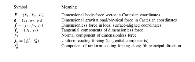


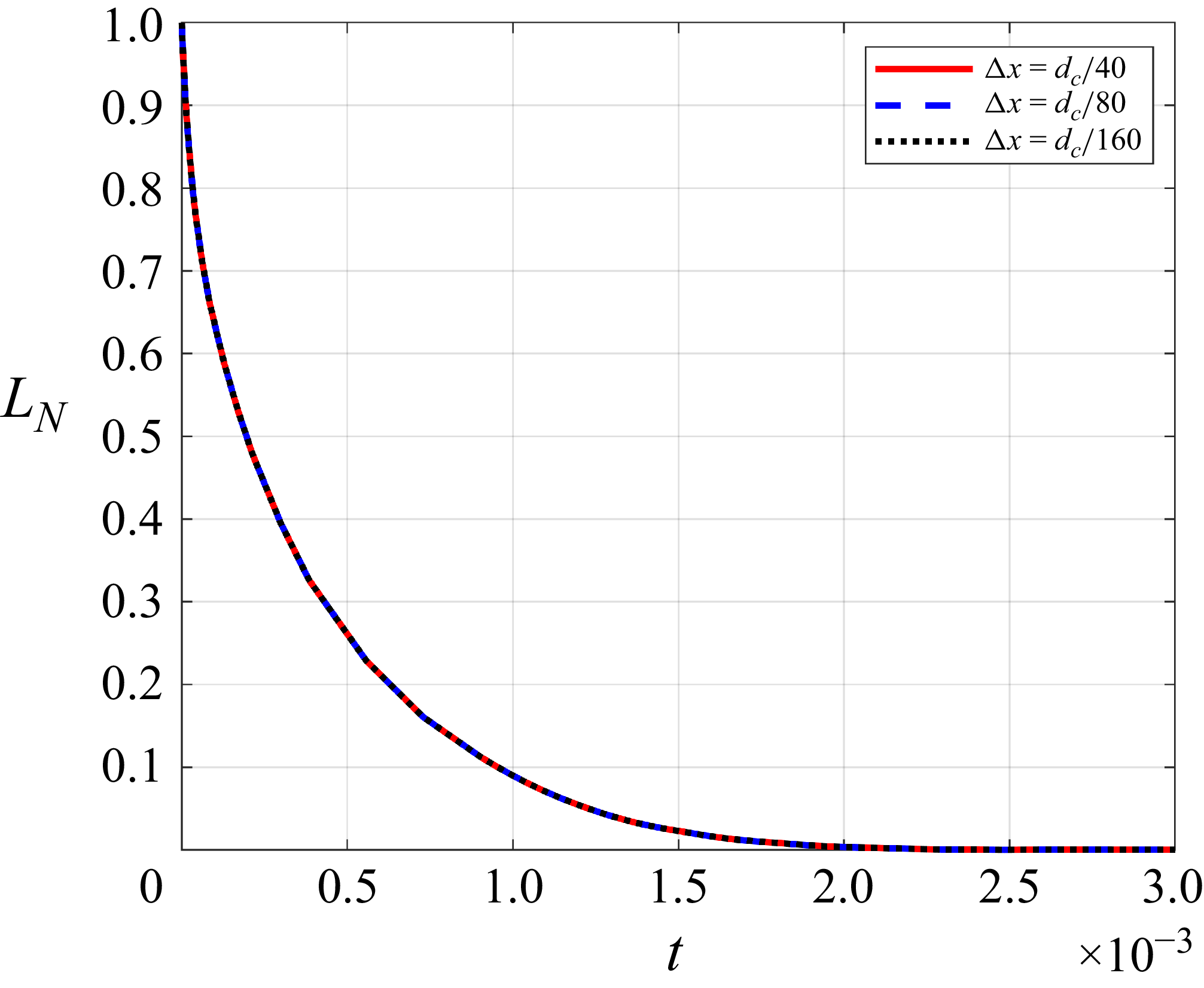


 Open access

