Refine search
Actions for selected content:
2327 results in Pattern Recognition and Machine Learning
Frontmatter
-
- Book:
- Bayesian Optimization
- Published online:
- 25 January 2023
- Print publication:
- 09 February 2023, pp i-iv
-
- Chapter
- Export citation
Preface
-
- Book:
- Bayesian Optimization
- Published online:
- 25 January 2023
- Print publication:
- 09 February 2023, pp ix-xvi
-
- Chapter
- Export citation
9 - implementation
-
- Book:
- Bayesian Optimization
- Published online:
- 25 January 2023
- Print publication:
- 09 February 2023, pp 201-212
-
- Chapter
- Export citation
B - methods for approximate bayesian inference
-
- Book:
- Bayesian Optimization
- Published online:
- 25 January 2023
- Print publication:
- 09 February 2023, pp 301-306
-
- Chapter
- Export citation
10 - theoretical analysis
-
- Book:
- Bayesian Optimization
- Published online:
- 25 January 2023
- Print publication:
- 09 February 2023, pp 213-244
-
- Chapter
- Export citation
8 - computing policies with gaussian processes
-
- Book:
- Bayesian Optimization
- Published online:
- 25 January 2023
- Print publication:
- 09 February 2023, pp 157-200
-
- Chapter
- Export citation
12 - a brief history of bayesian optimization
-
- Book:
- Bayesian Optimization
- Published online:
- 25 January 2023
- Print publication:
- 09 February 2023, pp 287-294
-
- Chapter
- Export citation
2 - gaussian processes
-
- Book:
- Bayesian Optimization
- Published online:
- 25 January 2023
- Print publication:
- 09 February 2023, pp 15-44
-
- Chapter
- Export citation
A - the gaussian distribution
-
- Book:
- Bayesian Optimization
- Published online:
- 25 January 2023
- Print publication:
- 09 February 2023, pp 295-300
-
- Chapter
- Export citation
5 - decision theory for optimization
-
- Book:
- Bayesian Optimization
- Published online:
- 25 January 2023
- Print publication:
- 09 February 2023, pp 87-108
-
- Chapter
- Export citation
6 - utility functions for optimization
-
- Book:
- Bayesian Optimization
- Published online:
- 25 January 2023
- Print publication:
- 09 February 2023, pp 109-122
-
- Chapter
- Export citation
4 - model assessment, selection, and averaging
-
- Book:
- Bayesian Optimization
- Published online:
- 25 January 2023
- Print publication:
- 09 February 2023, pp 67-86
-
- Chapter
- Export citation
7 - common bayesian optimization policies
-
- Book:
- Bayesian Optimization
- Published online:
- 25 January 2023
- Print publication:
- 09 February 2023, pp 123-156
-
- Chapter
- Export citation
Contents
-
- Book:
- Bayesian Optimization
- Published online:
- 25 January 2023
- Print publication:
- 09 February 2023, pp v-viii
-
- Chapter
- Export citation
references
-
- Book:
- Bayesian Optimization
- Published online:
- 25 January 2023
- Print publication:
- 09 February 2023, pp 331-352
-
- Chapter
- Export citation
Index
-
- Book:
- Bayesian Optimization
- Published online:
- 25 January 2023
- Print publication:
- 09 February 2023, pp 353-358
-
- Chapter
- Export citation
D - annotated bibliography of applications
-
- Book:
- Bayesian Optimization
- Published online:
- 25 January 2023
- Print publication:
- 09 February 2023, pp 313-330
-
- Chapter
- Export citation

Machine Learning for Engineers
-
- Published online:
- 25 January 2023
- Print publication:
- 03 November 2022
-
- Textbook
- Export citation

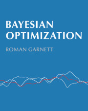
Bayesian Optimization
-
- Published online:
- 25 January 2023
- Print publication:
- 09 February 2023

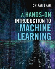
A Hands-On Introduction to Machine Learning
-
- Published online:
- 20 January 2023
- Print publication:
- 29 December 2022
-
- Textbook
- Export citation
