


1. Introduction
What’s past is prologue—unavoidably, the present is shaped by what has already occurred. The current state of the world is indebted to our history. Our actions, behaviors, and decisions are both precursory and prescriptive to those that follow, and this can be observed across a variety of different scenarios. For example, the spread of an infectious disease is accelerated as more people become sick and dampened as they recover. In finance, a flurry of recent transactions can prompt new buyers or sellers to enter a market. On social media platforms, as more and more users interact with a post it can become trending or viral and thus be broadcast to an even larger audience.
Self-exciting processes are an intriguing family of stochastic models in which the history of events influences the future. The paper [Reference Hawkes36] introduced the concept of self-excitement—defining what is now known as the Hawkes process, a model in which ‘the current intensity of events is determined by events in the past’. That is, the Hawkes process is a stochastic-intensity point process that depends on the history of the point process itself. The rate of new event occurrences increases as each event occurs. As time passes between occurrences, the intensity is governed by a deterministic excitement kernel. Most often, this kernel is specified so that the intensity jumps upward at event epochs and strictly decreases in the interim. In this way, occurrences beget occurrences; hence the term ‘self-exciting’. Unlike in the Poisson process, disjoint increments are not independent in sample paths of the Hawkes process. Instead, they are positively correlated and, by definition, the events of the former influence the events of the latter. Furthermore, the Hawkes process is known to be over-dispersed—meaning that its variance is larger than its mean—which is commonly found in real-world data, whereas the Poisson process has equal mean and variance.
Because of the practical relevance of these model features, self-exciting processes have been used in a wide variety of applications, many of which are quite recent additions to the literature. Seismology was among the first domains to incorporate these models, for example in [Reference Ogata51], as the occurrence of an earthquake increases the risk of subsequent seismic activity in the form of aftershocks. Finance has since followed as a popular application and is now perhaps the most active area of work. In these studies, self-excitement is used to capture the often contagious nature of financial activity; see e.g. [Reference At-Sahalia, Cacho-Diaz and Laeven2, Reference Azizpour, Giesecke and Schwenkler4, Reference Bacry, Delattre, Hoffmann and Muzy5, Reference Bacry and Muzy7, Reference Da Fonseca and Zaatour15, Reference Errais, Giesecke and Goldberg24, Reference Gao, Zhou and Zhu28, Reference Rambaldi, Bacry and Lillo53, Reference Wu, Rambaldi, Muzy and Bacry62]. Similarly, there have been many recent internet and social media scenarios that have been modeled using self-exciting processes, drawing upon the virality of modern web traffic. For example, see [Reference Farajtabar26, Reference Rizoiu54, Reference Rizoiu55]. Notably, this also includes use of Hawkes processes for constructing data-driven methods in the artificial intelligence and machine learning literatures, e.g. [Reference Du22, Reference Mei and Eisner50, Reference Xu, Luo and Zha63]. In an intriguing area of work, self-excitement has also been used to model interpersonal communication, for example in application to conversation audio recordings in [Reference Masuda, Takaguchi, Sato and Yano49] or in studying email correspondence in [Reference Halpin and De Boeck34, Reference Malmgren, Stouffer, Motter and Amaral47]. Hawkes processes have also recently been used to represent arrivals to service systems in queueing models, e.g. in [Reference Daw and Pender20, Reference Gao and Zhu29, Reference Gao and Zhu30, Reference Koops, Saxena, Boxma and Mandjes41]. This is of course not an exhaustive list of works in these areas, nor is it a complete account of all the modern applications of self-excitement. Examples of other notable uses include neuroscience [Reference Krumin, Reutsky and Shoham42, Reference Truccolo57], environmental management [Reference Gupta, Farajtabar, Dilkina and Zha32], public health [Reference Zino, Rizzo and Porfiri68], movie trailer generation [Reference Xu, Zhen and Zha64], energy conservation [Reference Li and Zha44], and industrial preventative maintenance [Reference Yan65].
As the variety of uses for self-excitement has continued to grow, the number of Hawkes process generalizations has kept pace. By modifying the definition of the Hawkes process in some way, the works in this generalized self-exciting process literature provide new perspectives on these concepts while also empowering and enriching applications. For example, [Reference Brémaud and Massoulié13] introduces a nonlinear Hawkes process that adapts the definition of the process intensity to feature a general, nonnegative function of the integration over the process history, as opposed to the linear form given originally. Similarly, the quadratic Hawkes process model given by [Reference Blanc, Donier and Bouchaud11] allows for excitation kernels that have quadratic dependence on the process history, rather than simply linear. This is also an example of a generalization motivated by application, as the authors seek to capture time-reversal asymmetry observed in financial data. As another finance-motivated generalization, [Reference Dassios and Zhao17] proposes the dynamic contagion process. This model can be thought of as a hybrid between a Hawkes process and a shot-noise process, as the stochastic intensity of the model features both self-excited and externally excited jumps. The authors take motivation from an application in credit risk, in which the dynamics are shaped both by the process history and by exogenous shocks. The affine point processes studied in e.g. [Reference Errais, Giesecke and Goldberg24, Reference Zhang, Blanchet, Giesecke and Glynn66, Reference Zhang, Glynn, Giesecke and Blanchet67] are also motivated by credit risk applications. The models in these works combine the self-exciting dynamics of Hawkes process with those of an affine jump-diffusion process, imbedding modeling concepts of feedback and dependency into the process intensity. An exact simulation procedure for the Hawkes process with Cox–Ingersoll–Ross (CIR) intensity, a generalization of the Hawkes process that is a special case of the affine point process, is shown in [Reference Dassios and Zhao18]. In that case, the authors discuss an application to portfolio loss processes.
There have also been several Hawkes process generalizations proposed in social media and data analytics contexts. For example, [Reference Rizoiu54] introduces a finite-population Hawkes process that couples self-excitement dynamics with those of the susceptible–infected–recovered (SIR) process. Drawing upon the use of the SIR process for the spread of both disease and ideas, the authors propose this SIR–Hawkes process as a method of studying information cascades. Similarly, [Reference Mei and Eisner50] introduces the neural Hawkes process as a new point process model in the machine learning literature. As the name suggests, this model combines self-excitement with concepts from neural networks. Specifically, a recurrent neural network effectively replaces the excitation kernel, governing the effect of the past events on the rate of future occurrences. In the literature for Bayesian nonparametric models, [Reference Du22] presents the Dirichlet–Hawkes process for topic clustering in document streams. In this case, the authors combine a Hawkes process and a Dirichlet process, so that the intensity of the stream of new documents is self-exciting while the type of each new document is determined by the Dirichlet process, leading to a preferential attachment structure among the document types.
In this paper, we propose the ephemerally self-exciting process (ESEP), a novel generalization of the Hawkes process. Rather than regulating the excitement through the gradual, deterministic decay provided by an excitation kernel function, we instead incorporate randomly timed down-jumps. We will refer to this random length of time as the arrival’s activity duration. The down-jumps are equal in size to the up-jumps, and between events the arrival rate does not change. Thus, this process increases in arrival rate upon each occurrence, and these increases are then mirrored some time later by decreases in the arrival rate once the activity duration expires. In this way, the self-excitement is ephemeral: it is only in effect as long as the excitement is active. Much of the body of this work will discuss how this ephemeral, piecewise constant self-excitement compares to the eternal but ever-decaying notion from Hawkes’s original definition. As we will see in our analysis, this new process is both a promising model of self-excitement and an explanation of its origins in natural phenomena.
1.1. Practical relevance
While this paper will not be focused on any one application, in this subsection we summarize several domain areas in which the models in this work can be applied. A natural example is in public health and the management of epidemics. For example, consider influenza. When a person becomes sick with the flu, she increases the rate of spread of the virus through her contact with others. This creates a self-exciting dynamic in the spread of the virus. However, a person only spreads a disease as long as she is contagious; once she has recovered she no longer has a direct effect on the rate of new infections. From a system-level perspective, the ESEP can thus be thought of as modeling the arrivals of new infections, capturing the self-exciting and ephemeral nature of sick patients. This motivates the use of this model as an arrival process to queueing models for healthcare, as the rate of arrivals to clinics serving patients with infectious diseases should depend on the number of people currently infected. The healthcare service can also be separately modeled, as an infinite-server queue may be a fitting representation for the number of infected individuals but the clinic itself likely has limited capacity. This concept of course extends to the modeling and management of any other viral disease, including the novel coronavirus that has caused the COVID-19 pandemic.
Of course, epidemic models need not be applied exclusively to disease spread. These same ideas can be used for information spread and product adoption, such as in the aforementioned Hawkes-infused models in [Reference Rizoiu54, Reference Zino, Rizzo and Porfiri68]. In these contexts, one can think of the duration in system as being the time a person actively promotes a concept or product. A single person only affects the self-excitement of the idea or product spread as long as she is in the system, which distinguishes this model from those in the aforementioned works. Epidemic models have also been used to study social issues, such as the contagious nature of imprisonment demonstrated by [Reference Lum, Swarup, Eubank and Hawdon46]. We discuss the relevance of ephemeral self-excitement for epidemics in detail in Subsection 3.3 by relating this model to the susceptible–infected–susceptible (SIS) process through a convergence in distribution. In fact, throughout Section 3 we establish connections from this process to other relevant stochastic models. This includes classical processes such as branching processes and random walks, as well as models popular both in Bayesian nonparametrics and in preferential attachment settings, such as the Dirichlet process and the Chinese restaurant process (CRP).
In the context of service systems, self-excitement can be motivated by the same rationale that inspires restaurants to seat customers at the tables by the windows. Potential new customers could choose to dine at the establishment because they can see others already eating there, taking an implicit recommendation from those already being served. This same example also motivates the ephemerality. After a customer seated by the window finishes her dinner and departs, any passing potential patron only sees an empty table; the implicit recommendation vanishes with the departing customer. A similar dynamic can be observed in online streaming platforms. For example, on popular music streaming services like Spotify and Apple Music, users can see what songs and albums have been recently played by their friends. If a user sees that many of her friends have listened to the same album recently, she may be more inclined to listen to it as well. However, this applies only as long as the word ‘recently’ does. If her friends don’t play the album within a certain amount of time, the platform will no longer promote the album to her in that fashion. Again, this displays the ephemerality of the underlying self-excitement: the album grows more attractive as more users listen to it, but only as long as those listens are ‘recent’ enough.
In finance, limit order books (LOBs) are among the many concepts that have been modeled using Hawkes process, for example in [Reference Bacry, Jaisson and Muzy6, Reference Rambaldi, Bacry and Lillo53]. LOBs have also been studied through queueing models, where one can model the state of the LOB (or, more specifically, the number of unresolved bids and asks) as the length of a queueing process. Moreover, there has been recent work that models this process as not just a queue, but a queue with Hawkes process arrivals; for example see [Reference Gao and Zhu29, Reference Guo, Ruan and Zhu31]. Conceptually, the self-excitement may arise from traders reacting to the activity of other traders, creating runs of transactions. However, the desire not to act on stale information may mean that this excitement lasts only as long as trades are actively being conducted. In fact, the idea of the self-excitement in LOB models being ‘queue-reactive’ has just very recently been considered by [Reference Wu, Rambaldi, Muzy and Bacry62], a work related to this one.
One can also consider failures in a mechanical system as an application of this model. For example, consider a network of water pipes. When one pipe breaks or bursts, it can place stress on the pipes connected to it. This stress may then cause further failures within the pipe network. However, once the pipe is properly repaired, it should no longer place strain on the surrounding components. Thus, the increase in pipe failure rate caused by a failure is only in effect until the repair occurs, inducing ephemeral self-excitement. The self-excitement (albeit without the ephemerality) arising in this scenario was modeled using Hawkes processes in [Reference Yan65], which includes an empirical study. A similar problem for electrical systems is considered in [Reference Ertekin, Rudin and McCormick25]. The reactive point process considered in that work is perhaps the model most similar to the ones studied herein, as the rate of new power failures both increases at the prior failure times and decreases upon inspection or repair. However, a key difference is that in [Reference Ertekin, Rudin and McCormick25], the authors treat the inspection times as controlled by management, whereas in this paper the model is fully stochastic and thus the repair durations are random. Regardless, that work is an excellent example of how generalized self-exciting processes can be used to shape practical policy. Because power outages have significant and wide-reaching consequences, it is critical to understand the interdependency between electrical grid failures and to study the ESEP that arises from them.
1.2. Organization and contributions of paper
Let us now detail the remainder of this paper’s organization, as well as the contributions therein.
-
In Section 2, we define the ephemerally self-exciting process (ESEP), a Markovian model for self-excitement that lasts for only a finite amount of time. After defining the model, we develop fundamental distributional quantities and compare the ESEP to the Hawkes process.
-
In Section 3, we relate the ESEP to many other important and well-known stochastic processes. This includes branching processes, which gives us further comparisons between the Hawkes process and the ESEP, models for preferential attachment and Bayesian statistics, and epidemic models. The lattermost of these motivates the ESEP as a representation for the times of infection within an epidemic, and this also provides a formal link between the conceptually similar concepts of epidemics and self-excitement.
-
In Section 4, we broaden our exploration of ephemeral self-excitement to non-Markovian models with general activity durations and batches of arrivals. In this general setting, we establish a limit theorem providing an alternate construction of general Hawkes processes. This batch scaling limit thus yields intuition for the observed occurrence of self-excitement in natural phenomena and stands as a fundamental cornerstone for studying such processes.
In addition to these main avenues of study, we also have extensive auxiliary analysis housed in this paper’s appendix. Appendix A contains lemmas and side results that support our analysis but are outside the main narrative. In Appendix B, we explore a model that is a hybrid between the ESEP and the Hawkes process, in that it regulates the excitement with both down-jumps and decay. Appendix C is devoted to a finite-capacity version of the ESEP, in which arrivals that would put the active number in system above the capacity are blocked from occurring. Finally, Appendix D contains an algebraically cumbersome proof of a result from Section 2.
2. Modeling ephemeral self-excitement
We begin this paper by defining our ephemerally self-exciting model and conducting an initial analysis of some fundamental quantities, including the transient moment generating function and the steady-state distribution. Before doing so, though, let us first review the Hawkes process, which is the original self-exciting probability model.
2.1. Preliminary models and concepts
Introduced and pioneered through the series of papers [Reference Hawkes35–Reference Hawkes and Oakes37], the Hawkes process is a stochastic-intensity point process in which the current rate of arrivals is dependent on the history of the arrival process itself. Formally, this is defined as follows: let $(\lambda_t, N_{t,\lambda})$
be an intensity and counting process pair such that
$(\lambda_t, N_{t,\lambda})$
be an intensity and counting process pair such that
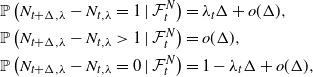 \begin{align*}\mathbb{P}\left( N_{t+\Delta,\lambda} - N_{t,\lambda} = 1 \mid \mathcal{F}^N_t \right) &= \lambda_t \Delta + o(\Delta), \\\mathbb{P}\left( N_{t+\Delta,\lambda} - N_{t,\lambda} > 1 \mid \mathcal{F}^N_t \right) &= o(\Delta), \\\mathbb{P}\left( N_{t+\Delta,\lambda} - N_{t,\lambda} = 0 \mid \mathcal{F}^N_t \right) &= 1 - \lambda_t \Delta + o(\Delta),\end{align*}
where $\mathcal{F}^N_t$
is the filtration of
$\mathcal{F}^N_t$
is the filtration of $N_{t,\lambda}$
up to time t and
$N_{t,\lambda}$
up to time t and $\lambda_t$
is given by
$\lambda_t$
is given by
 \begin{align*}\lambda_t = \lambda^* + \int_{-\infty}^t g(t-u) \textrm{d}N_{u,\lambda},\end{align*}
where $\lambda^* > 0$
and
$\lambda^* > 0$
and $g\, :\, \mathbb{R}^+ \to \mathbb{R}^+$
is such that
$g\, :\, \mathbb{R}^+ \to \mathbb{R}^+$
is such that $\int_0^\infty g(x) \textrm{d}x < 1$
. Through this definition, the intensity
$\int_0^\infty g(x) \textrm{d}x < 1$
. Through this definition, the intensity $\lambda_t$
captures the history of the arrival process up to time t. Thus,
$\lambda_t$
captures the history of the arrival process up to time t. Thus, $\lambda_t$
encapsulates the sequence of past events and uses it to determine the rate of future occurrences. We refer to
$\lambda_t$
encapsulates the sequence of past events and uses it to determine the rate of future occurrences. We refer to $\lambda^*$
as the baseline intensity and
$\lambda^*$
as the baseline intensity and $g({\cdot})$
as the excitation kernel. The baseline intensity represents an underlying stationary arrival rate, and the excitation kernel governs the effect that the history of the process has on the current intensity. A common modeling choice is to set
$g({\cdot})$
as the excitation kernel. The baseline intensity represents an underlying stationary arrival rate, and the excitation kernel governs the effect that the history of the process has on the current intensity. A common modeling choice is to set $g(x) = \alpha e^{-\beta x}$
, where
$g(x) = \alpha e^{-\beta x}$
, where $\beta > \alpha > 0$
. This is often referred to as the ‘exponential’ kernel, and it is perhaps the most widely used form of the Hawkes process. In this case,
$\beta > \alpha > 0$
. This is often referred to as the ‘exponential’ kernel, and it is perhaps the most widely used form of the Hawkes process. In this case, $(\lambda_t, N_{t,\lambda})$
is a Markov process obeying the stochastic differential equation
$(\lambda_t, N_{t,\lambda})$
is a Markov process obeying the stochastic differential equation
 \begin{align*}\textrm{d}\lambda_t = \beta(\lambda^* - \lambda_t)\textrm{d}t + \alpha \textrm{d}N_{t,\lambda}.\end{align*}
That is, at arrival epochs $\lambda_t$
jumps upward by the amount
$\lambda_t$
jumps upward by the amount $\alpha$
and the
$\alpha$
and the $N_{t,\lambda}$
increases by 1; between arrivals
$N_{t,\lambda}$
increases by 1; between arrivals $\lambda_t$
decays exponentially at rate
$\lambda_t$
decays exponentially at rate $\beta$
towards the baseline intensity
$\beta$
towards the baseline intensity $\lambda^*$
. Thus, each arrival increases the likelihood of additional arrivals occurring soon afterwards—hence, it self-excites. This form of the Hawkes process is also often alternatively stated with an initial value for
$\lambda^*$
. Thus, each arrival increases the likelihood of additional arrivals occurring soon afterwards—hence, it self-excites. This form of the Hawkes process is also often alternatively stated with an initial value for $\lambda_t$
, say
$\lambda_t$
, say $\lambda_0 \geq \lambda^*$
. In this case, the intensity can be expressed as
$\lambda_0 \geq \lambda^*$
. In this case, the intensity can be expressed as
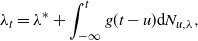
 \begin{align*}\lambda_t=\lambda^*+(\lambda_0 - \lambda^*)e^{-\beta t}+\alpha\int_{0}^t e^{-\beta (t-u)} \textrm{d}N_{u,\lambda}.\end{align*}
Additional overview of the Hawkes process with the exponential kernel can be found in Section 2 of [Reference Daw and Pender20]. Another common choice for excitation kernel is the ‘power-law’ kernel $g(x) = \frac{k}{(c+x)^p}$
, where
$g(x) = \frac{k}{(c+x)^p}$
, where $k > 0$
,
$k > 0$
, $c > 0$
, and
$c > 0$
, and $p > 0$
. This kernel was originally popularized in seismology [Reference Ogata51].
$p > 0$
. This kernel was originally popularized in seismology [Reference Ogata51].
2.2. Defining the ephemerally self-exciting process
As we have discussed in the introduction, a plethora of natural phenomena exhibit self-exciting features but only for a finite amount of time. This prompts the notion of ephemeral self-excitement. By comparison to the traditional Hawkes process we have reviewed in Subsection 2.1, we seek a model in which a new occurrence increases the arrival rate only so long as the newly entered entity remains active in the system. Thus, we now define the ephemerally self-exciting process (ESEP), which trades the Hawkes process’s eternal decay for randomly drawn expiration times. Moreover, in the following Markovian model, exponential decay is replaced with exponentially distributed durations. In Section 4, we extend these concepts to generally distributed service. As another generalization, in Appendix B we consider a Markovian model with both decay and down-jumps. For now, we explore the effects of ephemerality through the ESEP model in Definition 1.
Definition 1.
(Ephemerally self-exciting process.) For times $t \geq 0$
, a baseline intensity
$t \geq 0$
, a baseline intensity $\eta^* > 0$
, intensity jump size
$\eta^* > 0$
, intensity jump size $\alpha > 0$
, and expiration rate
$\alpha > 0$
, and expiration rate $\beta > 0$
, let
$\beta > 0$
, let $N_t$
be a counting process with stochastic intensity
$N_t$
be a counting process with stochastic intensity $\eta_t$
such that
$\eta_t$
such that
 \begin{align}\eta_t = \eta^* + \alpha Q_t,\end{align}
where $Q_t$
is incremented with
$Q_t$
is incremented with $N_t$
and then is depleted at unit down-jumps according to the rate
$N_t$
and then is depleted at unit down-jumps according to the rate $\beta Q_t$
. We say that
$\beta Q_t$
. We say that $(\eta_t, N_t)$
is an ephemerally self-exciting process (ESEP).
$(\eta_t, N_t)$
is an ephemerally self-exciting process (ESEP).
We will assume that $\eta_0$
and
$\eta_0$
and $Q_0$
are known initial values such that
$Q_0$
are known initial values such that $\eta_0 = \eta^* + \alpha Q_0$
. In addition to this definition, one could also describe the ESEP through its dynamics. In particular, the behavior of this process can be summarily cast through the life cycle of its arrivals:
$\eta_0 = \eta^* + \alpha Q_0$
. In addition to this definition, one could also describe the ESEP through its dynamics. In particular, the behavior of this process can be summarily cast through the life cycle of its arrivals:
-
i. At each arrival, the arrival rate $\eta_t$
increases by
$\alpha$
.
$\eta_t$
increases by
$\alpha$
. -
ii. Each arrival remains active for an activity duration drawn from an independent and identically distributed (i.i.d.) sequence of exponential random variables with rate
$\beta$
. -
iii. At the expiration of a given activity duration,
$\eta_t$
decreases by
$\alpha$
.


The ephemerality of the ESEP is embodied by this cycle. Because arrivals only contribute to the intensity for the length of their activity duration, their effect on the process’s excitation vanishes when this clock expires. Furthermore, there is an affine relationship between the number of active ‘exciters’—meaning unexpired arrivals still causing excitation—and the intensity, i.e. $\eta_t = \eta^* + \alpha Q_t$
. Thus, we could also track the arrival rate through
$\eta_t = \eta^* + \alpha Q_t$
. Thus, we could also track the arrival rate through $Q_t$
in place of
$Q_t$
in place of $\eta_t$
and still have full understanding of this process. This also means that results are readily transferrable between these two processes; we will often make use of this fact.
$\eta_t$
and still have full understanding of this process. This also means that results are readily transferrable between these two processes; we will often make use of this fact.
Because the ESEP is quite parsimonious, there are many alternative perspectives we could take to gain additional understanding of it. For example, one could consider $Q_t$
a Markovian queueing system with infinitely many servers and a state-dependent arrival rate. Equivalently, one could also describe the ESEP as a Markov chain on the nonnegative integers where transitions at state i are to
$Q_t$
a Markovian queueing system with infinitely many servers and a state-dependent arrival rate. Equivalently, one could also describe the ESEP as a Markov chain on the nonnegative integers where transitions at state i are to $i+1$
at rate
$i+1$
at rate $\eta^* + \alpha i$
and to
$\eta^* + \alpha i$
and to $i-1$
at rate
$i-1$
at rate $\mu i$
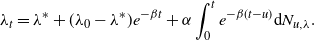
, with the counting process then defined as the epochs of the upward jumps in this chain. This Markov chain perspective certifies the existence and uniqueness of Definition 1. A visualization of this linear birth–death–immigration process is given in Figure 1. Stability for this chain occurs when
$\mu i$
, with the counting process then defined as the epochs of the upward jumps in this chain. This Markov chain perspective certifies the existence and uniqueness of Definition 1. A visualization of this linear birth–death–immigration process is given in Figure 1. Stability for this chain occurs when $\beta > \alpha$
; we will assume this henceforth, although of course it is not necessary for transient results. One could also view the ESEP as a generalization of Hawkes’s original definition where the excitation kernel function
$\beta > \alpha$
; we will assume this henceforth, although of course it is not necessary for transient results. One could also view the ESEP as a generalization of Hawkes’s original definition where the excitation kernel function $g({\cdot})$
is replaced with a randomly drawn indicator function that is different for each arrival. Each indicator function compares time to an independently drawn exponential random variable, and this perspective is closely aligned with our analysis in Section 3.
$g({\cdot})$
is replaced with a randomly drawn indicator function that is different for each arrival. Each indicator function compares time to an independently drawn exponential random variable, and this perspective is closely aligned with our analysis in Section 3.
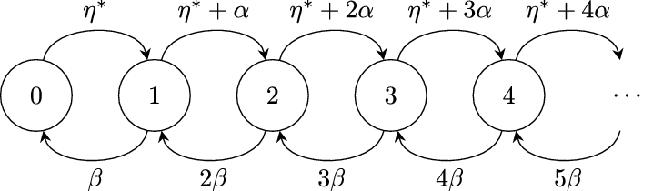
Figure 1. The transition diagram of the Markov chain for $Q_t$
.
$Q_t$
.
In the remainder of this subsection, let us now develop a few fundamental quantities for this stochastic process, particularly its intensity and active number in system, as these capture the self-exciting behavior of the process. First, in Proposition 1 we compute the transient moment generating function for the intensity $\eta_t$
. As we have noted, this can also be used to immediately derive the same transform for
$\eta_t$
. As we have noted, this can also be used to immediately derive the same transform for $Q_t$
, and the proof makes use of this fact.
$Q_t$
, and the proof makes use of this fact.
Proposition 1. Let $\eta_t = \eta^* + \alpha Q_t$
be the intensity of an ESEP with baseline intensity
$\eta_t = \eta^* + \alpha Q_t$
be the intensity of an ESEP with baseline intensity $\eta^* > 0$
, intensity jump
$\eta^* > 0$
, intensity jump $\alpha > 0$
, and expiration rate
$\alpha > 0$
, and expiration rate $\beta > \alpha$
. Then the moment generating function for
$\beta > \alpha$
. Then the moment generating function for $\eta_t$
is given by
$\eta_t$
is given by
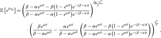 \begin{align*}{\mathbb{E}\left[e^{\theta \eta_t}\right]}&=\left(\frac{\beta - \alpha e^{\alpha\theta} - \beta \big(1-e^{\alpha\theta}\big)e^{-(\beta - \alpha)t}}{\beta - \alpha e^{\alpha\theta} - \alpha \big(1-e^{\alpha\theta}\big)e^{-(\beta - \alpha)t}}\right)^{\!\frac{\eta_0 - \eta^*}{\alpha}}\\&\qquad \cdot \left(\frac{\beta e^{\alpha \theta}}{\beta - \alpha e^{\alpha\theta}}-\frac{\alpha e^{\alpha \theta}}{\beta - \alpha e^{\alpha\theta}}\left(\frac{\beta - \alpha e^{\alpha\theta} - \beta \big(1-e^{\alpha\theta}\big)e^{-(\beta - \alpha)t}}{\beta - \alpha e^{\alpha\theta} - \alpha \big(1-e^{\alpha\theta}\big)e^{-(\beta - \alpha)t}}\right)\right)^{\!\frac{\eta^*}{\alpha}},\end{align*}
for all $t \geq 0$
and
$t \geq 0$
and $\theta < \frac{1}{\alpha}\log\left(\frac{\beta}{\alpha}\right)$
.
$\theta < \frac{1}{\alpha}\log\left(\frac{\beta}{\alpha}\right)$
.
Proof. We will approach this through the perspective of the active number in system, $Q_t$
. Using Lemma 2, we have that the probability generating function for
$Q_t$
. Using Lemma 2, we have that the probability generating function for $Q_t$
, say
$Q_t$
, say $\mathcal{P}(z,t) = {\mathbb{E}\!\left[z^{Q_t}\right]}$
for
$\mathcal{P}(z,t) = {\mathbb{E}\!\left[z^{Q_t}\right]}$
for $z \in [0,1]$
, is given by the solution to the following partial differential equation (PDE):
$z \in [0,1]$
, is given by the solution to the following partial differential equation (PDE):
 \begin{align*}\frac{\partial}{\partial t}{\mathbb{E}\big[z^{Q_t}\big]}&={\mathbb{E}\!\left[\left(\eta^* + \alpha Q_t\right)\left(z^2 - z\right)z^{Q_t - 1} + \beta Q_t \left(1 - z\right)z^{Q_t - 1}\right]},\end{align*}
which is equivalently expressed by
 \begin{align*}\frac{\partial}{\partial t}\mathcal{P}(z,t)&=\eta^* \left(z - 1\right)\mathcal{P}(z,t)+\left(\alpha \left(z^2 - z\right)+\beta\! \left(1 - z\right)\right)\frac{\partial}{\partial z}\mathcal{P}(z,t),\end{align*}
with initial condition $\mathcal{P}(z,0) = z^{Q_0}$
. The solution to this initial value problem is given by
$\mathcal{P}(z,0) = z^{Q_0}$
. The solution to this initial value problem is given by
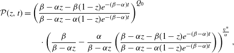 \begin{align*}\mathcal{P}(z,t)&=\left(\frac{\beta - \alpha z - \beta (1-z)e^{-(\beta - \alpha)t}}{\beta - \alpha z - \alpha (1-z)e^{-(\beta - \alpha)t}}\right)^{Q_0}\\&\qquad \cdot \left(\frac{\beta}{\beta - \alpha z}-\frac{\alpha}{\beta - \alpha z}\left(\frac{\beta - \alpha z - \beta (1-z)e^{-(\beta - \alpha)t}}{\beta - \alpha z - \alpha (1-z)e^{-(\beta - \alpha)t}}\right)\right)^{\!\frac{\eta^*}{\alpha}},\end{align*}
yielding the probability generating function for $Q_t$
. By setting
$Q_t$
. By setting $z = e^{\theta}$
we obtain the moment generating function. Finally, using the affine relationship
$z = e^{\theta}$
we obtain the moment generating function. Finally, using the affine relationship $\eta_t = \eta^* + \alpha Q_t$
, we have that
$\eta_t = \eta^* + \alpha Q_t$
, we have that
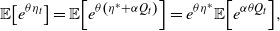 \begin{align*}{\mathbb{E}\!\left[e^{\theta \eta_t}\right]}={\mathbb{E}\!\left[e^{\theta \left(\eta^* + \alpha Q_t\right)}\right]}=e^{\theta \eta^*}{\mathbb{E}\!\left[e^{\alpha \theta Q_t}\right]},\end{align*}
with $\eta_0 = \eta^* + \alpha Q_0$
.
$\eta_0 = \eta^* + \alpha Q_0$
.
As we have mentioned, this Markov chain can be shown to be stable for $\beta > \alpha$
through standard techniques. Thus, using the moment generating function from Proposition 1, we can find the steady-state distributions of the intensity and the active number in system by taking the limit of t. We can quickly observe that this leads to a negative binomial distribution, as we state in Theorem 1. Because of the varying definitions of the negative binomial distribution, we state the probability mass function explicitly.
$\beta > \alpha$
through standard techniques. Thus, using the moment generating function from Proposition 1, we can find the steady-state distributions of the intensity and the active number in system by taking the limit of t. We can quickly observe that this leads to a negative binomial distribution, as we state in Theorem 1. Because of the varying definitions of the negative binomial distribution, we state the probability mass function explicitly.
Theorem 1. Let $\eta_t = \eta^* + \alpha Q_t$
be an ESEP with baseline intensity
$\eta_t = \eta^* + \alpha Q_t$
be an ESEP with baseline intensity $\eta^* > 0$
, intensity jump
$\eta^* > 0$
, intensity jump $\alpha > 0$
, and expiration rate
$\alpha > 0$
, and expiration rate $\beta > \alpha$
. Then the active number in system in steady state follows a negative binomial distribution with parameters
$\beta > \alpha$
. Then the active number in system in steady state follows a negative binomial distribution with parameters $\frac{\alpha}{\beta}$
and
$\frac{\alpha}{\beta}$
and $\frac{\eta^*}{\alpha}$
, which is to say that the steady-state probability mass function is
$\frac{\eta^*}{\alpha}$
, which is to say that the steady-state probability mass function is
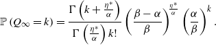 \begin{align}\mathbb{P}\left( Q_\infty = k \right)&=\frac{\Gamma\left(k + \frac{\eta^*}{\alpha}\right)}{\Gamma\left(\frac{\eta^*}{\alpha}\right) k! }\left(\frac{\beta - \alpha}{\beta}\right)^{\!\frac{\eta^*}{\alpha}}\left(\frac{\alpha}{\beta}\right)^k.\end{align}
Consequently, the steady-state distribution of the intensity is given by a shifted and scaled negative binomial with parameters $\frac{\alpha}{\beta}$
and
$\frac{\alpha}{\beta}$
and $\frac{\eta^*}{\alpha}$
, shifted by
$\frac{\eta^*}{\alpha}$
, shifted by $\eta^*$
and scaled by
$\eta^*$
and scaled by $\alpha$
.
$\alpha$
.
Proof. Using Proposition 1, we can see that the steady-state moment generating function of $Q_t$
is given by
$Q_t$
is given by
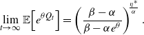 \begin{align*}\lim_{t\to\infty} {\mathbb{E}\!\left[e^{\theta Q_t}\right]}=\left(\frac{\beta-\alpha}{\beta - \alpha e^{\theta}}\right)^{\!\frac{\eta^*}{\alpha}}.\end{align*}
We can observe that this steady-state moment generating function is equivalent to that of a negative binomial. By the affine transformation $\eta_t = \eta^* + \alpha Q_t$
, we find the steady-state distribution for the intensity.
$\eta_t = \eta^* + \alpha Q_t$
, we find the steady-state distribution for the intensity.
The negative binomial distribution presented in Theorem 1 allows for $\frac{\eta^*}{\alpha}$
to take on any positive real value; integrality is not required. If
$\frac{\eta^*}{\alpha}$
to take on any positive real value; integrality is not required. If $\frac{\eta^*}{\alpha}$
is in fact an integer, then the gamma functions will match the corresponding factorial functions and this ratio of factorials will simplify to a binomial coefficient, reproducing the most familiar form of the negative binomial distribution. In this case,
$\frac{\eta^*}{\alpha}$
is in fact an integer, then the gamma functions will match the corresponding factorial functions and this ratio of factorials will simplify to a binomial coefficient, reproducing the most familiar form of the negative binomial distribution. In this case, $\frac{\eta^*}{\alpha}$
can be interpreted as the number of failures upon which an experiment is stopped, where the success probability is
$\frac{\eta^*}{\alpha}$
can be interpreted as the number of failures upon which an experiment is stopped, where the success probability is $\frac{\alpha}{\beta}$
and
$\frac{\alpha}{\beta}$
and $k + \frac{\eta^*}{\alpha}$
is the total number of trials.
$k + \frac{\eta^*}{\alpha}$
is the total number of trials.
Let us pause to note that this explicit characterization of the steady-state intensity is already an advantage of the ESEP over the traditional Markovian Hawkes process, for which there is not a closed-form intensity stationary distribution available. As a consequence of Theorem 1, we can observe that the steady-state mean of the intensity is $\eta_\infty \,:\!=\, \frac{\beta \eta^*}{\beta - \alpha}$
. Interestingly, this would also be the steady-state mean of the Hawkes process when given the same baseline intensity, the same intensity jump size, and an exponential decay rate equal to the rate of expiration. This leads us to ponder how the processes would otherwise compare when given equivalent parameters. In Proposition 2 we find that although this equivalence of means extends to transient settings, for all higher moments the ESEP dominates the Hawkes process in terms of both the intensity and the counting process.
$\eta_\infty \,:\!=\, \frac{\beta \eta^*}{\beta - \alpha}$
. Interestingly, this would also be the steady-state mean of the Hawkes process when given the same baseline intensity, the same intensity jump size, and an exponential decay rate equal to the rate of expiration. This leads us to ponder how the processes would otherwise compare when given equivalent parameters. In Proposition 2 we find that although this equivalence of means extends to transient settings, for all higher moments the ESEP dominates the Hawkes process in terms of both the intensity and the counting process.
Proposition 2. Let $(\eta_t, N_{t,\eta})$
be an ESEP intensity and counting process pair with jump size
$(\eta_t, N_{t,\eta})$
be an ESEP intensity and counting process pair with jump size $\alpha > 0$
, expiration rate
$\alpha > 0$
, expiration rate $\beta > \alpha$
, and baseline intensity
$\beta > \alpha$
, and baseline intensity $\eta^* > 0$
. Similarly, let
$\eta^* > 0$
. Similarly, let $(\lambda_t, N_{t,\lambda})$
be a Hawkes process intensity and counting process pair with jump size
$(\lambda_t, N_{t,\lambda})$
be a Hawkes process intensity and counting process pair with jump size $\alpha > 0$
, decay rate
$\alpha > 0$
, decay rate $\beta > 0$
, and baseline intensity
$\beta > 0$
, and baseline intensity $\eta^* > 0$
. Then, if the two processes have equal initial values, their means will satisfy
$\eta^* > 0$
. Then, if the two processes have equal initial values, their means will satisfy
 \begin{align}&{\mathbb{E}\!\left[\lambda_t\right]} = {\mathbb{E}\!\left[\eta_t\right]},&&{\mathbb{E}\!\left[N_{t,\lambda}\right]} = {\mathbb{E}\!\left[N_{t,\eta}\right]},\end{align}
and for $m \geq 2$
their mth moments are ordered so that
$m \geq 2$
their mth moments are ordered so that
 \begin{align}&{\mathbb{E}\!\left[\lambda_t^m\right]} \leq {\mathbb{E}\!\left[\eta_t^m\right]},&&{\mathbb{E}\!\left[N_{t,\lambda}^m\right]} \leq {\mathbb{E}\!\left[N_{t,\eta}^m\right]},\end{align}
for all time $t \geq 0$
.
$t \geq 0$
.
Proof. Let us start with the means. For the intensities, we can note that these are given by the solutions to
 \begin{align*}\frac{\textrm{d}}{\textrm{d}t}{\mathbb{E}\!\left[\lambda_t\right]}=\alpha {\mathbb{E}\!\left[\lambda_t\right]} - \beta({\mathbb{E}\!\left[\lambda_t\right]} - \eta^*)\qquad \text{and}\qquad \frac{\textrm{d}}{\textrm{d}t}{\mathbb{E}\!\left[\eta_t\right]}=\alpha{\mathbb{E}\!\left[\eta_t\right]} - \beta \alpha\left( \frac{{\mathbb{E}\!\left[\eta_t\right]} - \eta^*}{\alpha} \right),\end{align*}
and through simplification one can quickly observe that these two ordinary differential equations (ODEs) are equivalent. Thus, because we have assumed that the processes have the same initial values, we find that ${\mathbb{E}\!\left[\lambda_t\right]} = {\mathbb{E}\!\left[\eta_t\right]}$
. Since
${\mathbb{E}\!\left[\lambda_t\right]} = {\mathbb{E}\!\left[\eta_t\right]}$
. Since
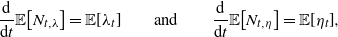 \begin{align*}\frac{\textrm{d}}{\textrm{d}t}{\mathbb{E}\!\left[N_{t,\lambda}\right]} = {\mathbb{E}\!\left[\lambda_t\right]}\qquad \text{and}\qquad \frac{\textrm{d}}{\textrm{d}t}{\mathbb{E}\!\left[N_{t,\eta}\right]} = {\mathbb{E}\!\left[\eta_t\right]},\end{align*}
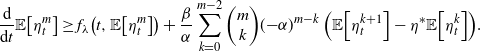
this equality immediately extends to the means of the counting processes as well. We will now use these equations for the means as the base cases for inductive arguments, beginning again with the intensities. For the inductive step, we will assume that the intensity moment ordering holds for moments 1 to $m-1$
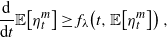
. The mth moment of the Hawkes process intensity is thus given by the solution to
$m-1$
. The mth moment of the Hawkes process intensity is thus given by the solution to
 \begin{align*}\frac{\textrm{d}}{\textrm{d}t}{\mathbb{E}\!\left[{\lambda_t}^m\right]}=\sum_{k=0}^{m-1} {\left(\begin{array}{c}m\\ k\end{array}\right)} {\mathbb{E}\!\left[{\lambda_t}^{k+1}\right]} \alpha^{m-k}-m \beta {\mathbb{E}\!\left[{\lambda_t}^m\right]}+m \beta \eta^{*} {\mathbb{E}\!\left[{\lambda_{t}}^{m-1}\right]}\,:\!=\,f_{\lambda}\left(t, {\mathbb{E}\!\left[{\lambda_t}^{m}\right]}\right),\end{align*}
where $f_\lambda\!\left(t, {\mathbb{E}\!\left[\lambda_t^{m}\right]}\right)$
is meant to capture that this ODE depends on the value of the mth moment and of the lower moments, which by the inductive hypothesis we take as known functions of the time t. Then, the mth moment of the ESEP intensity will satisfy
$f_\lambda\!\left(t, {\mathbb{E}\!\left[\lambda_t^{m}\right]}\right)$
is meant to capture that this ODE depends on the value of the mth moment and of the lower moments, which by the inductive hypothesis we take as known functions of the time t. Then, the mth moment of the ESEP intensity will satisfy
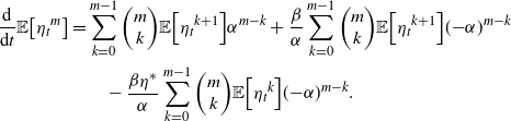 \begin{align*}\frac{\textrm{d}}{\textrm{d}t}{\mathbb{E}\!\left[{\eta_t}^m\right]}=&\sum_{k=0}^{m-1} {\left(\begin{array}{c}m\\ k\end{array}\right)} {\mathbb{E}\!\left[{\eta_t}^{k+1}\right]} \alpha^{m-k}+\frac{\beta}{\alpha}\sum_{k=0}^{m-1} {\left(\begin{array}{c}m\\ k\end{array}\right)} {\mathbb{E}\!\left[{\eta_t}^{k+1}\right]} ({-}\alpha)^{m-k}\\&\quad -\frac{\beta \eta^*}{\alpha}\sum_{k=0}^{m-1} {\left(\begin{array}{c}m\\ k\end{array}\right)} {\mathbb{E}\!\left[{\eta_t}^{k}\right]} ({-}\alpha)^{m-k}.\end{align*}
By pulling the $k = m-1$
terms off the top of each summation, we can re-express this ODE as
$k = m-1$
terms off the top of each summation, we can re-express this ODE as
 \begin{align*}\frac{\textrm{d}}{\textrm{d}t}{\mathbb{E}\!\left[\eta_t^m\right]}&=\sum_{k=0}^{m-1} {\left(\begin{array}{c}m\\ k\end{array}\right)} {\mathbb{E}\!\left[\eta_t^{k+1}\right]} \alpha^{m-k}-m\beta {\mathbb{E}\!\left[\eta_t^{m}\right]}+m\beta \eta^* {\mathbb{E}\!\left[\eta_t^{m-1}\right]}\\&\quad+\frac{\beta}{\alpha}\sum_{k=0}^{m-2} {\left(\begin{array}{c}m\\ k\end{array}\right)} ({-}\alpha)^{m-k}\left({\mathbb{E}\!\left[\eta_t^{k+1}\right]}-\eta^* {\mathbb{E}\!\left[\eta_t^{k}\right]}\right),\end{align*}
and through the definition of $f_\lambda({\cdot})$
and the inductive hypothesis, we can find the following lower bound:
$f_\lambda({\cdot})$
and the inductive hypothesis, we can find the following lower bound:
 \begin{align*}\frac{\textrm{d}}{\textrm{d}t}{\mathbb{E}\!\left[\eta_t^m\right]}&\geq f_\lambda\!\left(t, {\mathbb{E}\!\left[\eta_t^m\right]}\right)+\frac{\beta}{\alpha}\sum_{k=0}^{m-2} {\left(\begin{array}{c}m\\ k\end{array}\right)} ({-}\alpha)^{m-k}\left({\mathbb{E}\!\left[\eta_t^{k+1}\right]}-\eta^* {\mathbb{E}\!\left[\eta_t^{k}\right]}\right)\!.\end{align*}
This rightmost term can then be expressed as
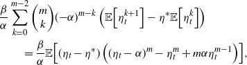 \begin{align*}&\frac{\beta}{\alpha}\sum_{k=0}^{m-2} {\left(\begin{array}{c}m\\ k\end{array}\right)} ({-}\alpha)^{m-k}\left({\mathbb{E}\!\left[\eta_t^{k+1}\right]}-\eta^* {\mathbb{E}\!\left[\eta_t^{k}\right]}\right)\\&\qquad =\frac{\beta}{\alpha}{\mathbb{E}\!\left[(\eta_t - \eta^*)\left((\eta_t - \alpha)^m-\eta_t^m+m \alpha \eta_t^{m-1}\right)\right]},\end{align*}
and we can now reason about the quantity inside the expectation. By definition, we have that $\eta_t \geq \eta^*$
with probability one, and furthermore we can observe that if
$\eta_t \geq \eta^*$
with probability one, and furthermore we can observe that if $\eta_t - \eta^* > 0$
, then
$\eta_t - \eta^* > 0$
, then $\eta_t \geq \eta^* + \alpha > \alpha$
. Thus, let us consider
$\eta_t \geq \eta^* + \alpha > \alpha$
. Thus, let us consider $(\eta_t - \alpha)^m-\eta_t^m+m \alpha \eta_t^{m-1}$
assuming
$(\eta_t - \alpha)^m-\eta_t^m+m \alpha \eta_t^{m-1}$
assuming $\eta_t > \alpha$
. Dividing through by
$\eta_t > \alpha$
. Dividing through by $\eta_t^m$
, we have the expression
$\eta_t^m$
, we have the expression
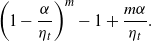 \begin{align}\left(1 - \frac{\alpha}{\eta_t}\right)^m-1+\frac{m \alpha}{ \eta_t}.\end{align}
Since $(1-x)^m - 1 + mx$
is equal to 0 at
$(1-x)^m - 1 + mx$
is equal to 0 at $x = 0$
and is non-decreasing on
$x = 0$
and is non-decreasing on $x \in [0,1)$
via a first-derivative check, we can note that (5) is nonnegative for all
$x \in [0,1)$
via a first-derivative check, we can note that (5) is nonnegative for all $\eta_t > \eta^*$
. Thus, we have that
$\eta_t > \eta^*$
. Thus, we have that
 \begin{align*}{\mathbb{E}\!\left[(\eta_t - \eta^*)\left((\eta_t - \alpha)^m-\eta_t^m+m \alpha \eta_t^{m-1}\right)\right]}\geq 0,\end{align*}
and by consequence,
 \begin{align*}\frac{\textrm{d}}{\textrm{d}t}{\mathbb{E}\!\left[\eta_t^m\right]}\geq f_\lambda\!\left(t, {\mathbb{E}\!\left[\eta_t^m\right]}\right),\end{align*}
completing the proof of the intensity moment ordering via Lemma 3. For the counting processes, let us again assume as an inductive hypothesis that the moment ordering holds for moments 1 through $m-1$
, with the mean equality serving as the base case. Then, the mth moment of the ESEP counting process will satisfy
$m-1$
, with the mean equality serving as the base case. Then, the mth moment of the ESEP counting process will satisfy
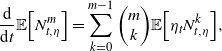 \begin{align*}\frac{\textrm{d}}{\textrm{d}t}{\mathbb{E}\!\left[N_{t,\eta}^m\right]}&=\sum_{k=0}^{m-1} {\left(\begin{array}{c}m\\ k\end{array}\right)} {\mathbb{E}\!\left[\eta_t N_{t,\eta}^k\right]},\end{align*}
and the ODE for the mth Hawkes counting process moment is analogous. By the Fortuin–Kasteleyn–Ginibre inequality, we can observe that
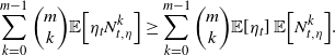 \begin{align*}\sum_{k=0}^{m-1} {\left(\begin{array}{c}m \\ k\end{array}\right)} {\mathbb{E}\!\left[\eta_t N_{t,\eta}^k\right]}\geq \sum_{k=0}^{m-1} {\left(\begin{array}{c}m \\ k\end{array}\right)} {\mathbb{E}\!\left[\eta_t\right]}\, {\mathbb{E}\!\left[N_{t,\eta}^k\right]}.\end{align*}
By the inductive hypothesis, we have that ${\mathbb{E}\!\left[N_{t,\eta}^k\right]} \geq {\mathbb{E}\!\left[N_{t,\lambda}^k\right]}$
for each
${\mathbb{E}\!\left[N_{t,\eta}^k\right]} \geq {\mathbb{E}\!\left[N_{t,\lambda}^k\right]}$
for each $k \leq m - 1$
, and thus we can observe that
$k \leq m - 1$
, and thus we can observe that
 \begin{align*}\sum_{k=0}^{m-1} {\left(\begin{array}{c}m\\ k\end{array}\right)} {\mathbb{E}\!\left[\eta_t\right]}\, {\mathbb{E}\!\left[N_{t,\eta}^k\right]}\geq \sum_{k=0}^{m-1} {\left(\begin{array}{c}m\\ k\end{array}\right)} {\mathbb{E}\!\left[\lambda_t\right]}\, {\mathbb{E}\!\left[N_{t,\lambda}^k\right]}.\end{align*}
Finally, by another application of Lemma 3, we have ${\mathbb{E}\!\left[N_{t,\lambda}^m\right]} \leq {\mathbb{E}\!\left[N_{t,\eta}^m\right]}$
.
${\mathbb{E}\!\left[N_{t,\lambda}^m\right]} \leq {\mathbb{E}\!\left[N_{t,\eta}^m\right]}$
.
The fact that the ESEP variance dominates the Hawkes variance should not be surprising, since the presence of both up- and down-jumps means that the ESEP sample paths should be subject to more abrupt changes. Nevertheless, this also shows that the ESEP is more over-dispersed than the Hawkes process is. This may be an attractive feature for data modeling. It is worth noting that matrix computations are available for all moments of these intensities via [Reference Daw and Pender21], through which one could use the method of moments to fit the processes to data.
2.3. The ephemerally self-exciting counting process
Thus far we have studied the intensity of the ESEP, as this process is by definition tracking the self-excitement. However, this excitation is manifested in the actual arrivals from the process, which are counted in $N_t$
. We now turn our attention to developing fundamental quantities for this counting process. To begin, we give the probability generating function of the counting process in closed form below in Proposition 3. One can note that by comparison, the generating functions of the Hawkes process are instead only expressible as functions of ODEs with no known closed-form solutions; see for example Subsection 3.5 of [Reference Daw and Pender20].
$N_t$
. We now turn our attention to developing fundamental quantities for this counting process. To begin, we give the probability generating function of the counting process in closed form below in Proposition 3. One can note that by comparison, the generating functions of the Hawkes process are instead only expressible as functions of ODEs with no known closed-form solutions; see for example Subsection 3.5 of [Reference Daw and Pender20].
Proposition 3. Let $N_t$
be the number of arrivals by time
$N_t$
be the number of arrivals by time $t \geq 0$
in an ESEP with baseline intensity
$t \geq 0$
in an ESEP with baseline intensity $\eta^* > 0$
, intensity jump
$\eta^* > 0$
, intensity jump $\alpha > 0$
, and expiration rate
$\alpha > 0$
, and expiration rate $\beta > \alpha$
. Then, for
$\beta > \alpha$
. Then, for $z \in [0,1]$
, the probability generating function of
$z \in [0,1]$
, the probability generating function of $N_t$
is given by
$N_t$
is given by
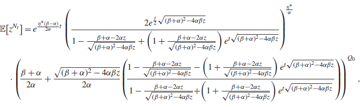 \begin{align}&{\mathbb{E}\!\left[z^{N_t}\right]}=e^{\frac{\eta^*(\beta-\alpha)}{2\alpha}t}\left(\frac{2e^{\frac{t}{2} \sqrt{(\beta+\alpha)^2 - 4\alpha\beta z}}}{1-\frac{ \beta+\alpha-2\alpha z}{\sqrt{(\beta+\alpha)^2 - 4\alpha\beta z}}+\left(1 + \frac{ \beta+\alpha-2\alpha z}{\sqrt{(\beta+\alpha)^2 - 4\alpha\beta z}}\right)e^{t \sqrt{(\beta+\alpha)^2 - 4\alpha\beta z}}}\right)^{\!\frac{\eta^*}{\alpha}}\nonumber \\&\quad\cdot \left(\!\frac{\beta + \alpha}{2\alpha}+\frac{\sqrt{(\beta+\alpha)^2 - 4\alpha\beta z}}{2\alpha}\!\left(\!\frac{1-\frac{ \beta+\alpha-2\alpha z}{\sqrt{(\beta+\alpha)^2 - 4\alpha\beta z}}-\left(1 + \frac{ \beta+\alpha-2\alpha z}{\sqrt{(\beta+\alpha)^2 - 4\alpha\beta z}}\right)e^{t \sqrt{(\beta+\alpha)^2 - 4\alpha\beta z}}}{1-\frac{ \beta+\alpha-2\alpha z}{\sqrt{(\beta+\alpha)^2 - 4\alpha\beta z}}\!+\!\left(1 + \frac{ \beta+\alpha-2\alpha z}{\sqrt{(\beta+\alpha)^2 - 4\alpha\beta z}}\right)e^{t \sqrt{(\beta+\alpha)^2 - 4\alpha\beta z}}}\right)\!\right)^{Q_0},\end{align}
where $Q_0$
is the active number in system at time 0.
$Q_0$
is the active number in system at time 0.
Proof. Because of the cumbersome length of some equations, the proof is given in Appendix D.
In addition to calculating the probability generating function, we can also find a matrix calculation for the transient probability mass function of the counting process. To do so, we recognize that the time until the next arrival occurs can be treated as the time to absorption in a continuous-time Markov chain. By building from this idea to construct a transition matrix for several successive arrivals, we find the form for the distribution given in Proposition 4.
Proposition 4. Let $N_t$
be the number of arrivals by time t in an ESEP with baseline intensity
$N_t$
be the number of arrivals by time t in an ESEP with baseline intensity $\eta^* > 0$
, intensity jump
$\eta^* > 0$
, intensity jump $\alpha > 0$
, and expiration rate
$\alpha > 0$
, and expiration rate $\beta > \alpha$
. Further, let
$\beta > \alpha$
. Further, let $Q_0 = k$
be the initial active number in system. Then for
$Q_0 = k$
be the initial active number in system. Then for $i \in \mathbb{N}$
, define the matrices
$i \in \mathbb{N}$
, define the matrices $\textbf{D}_i \in \mathbb{R}^{k + i + 1 \times k + i + 1}$
and
$\textbf{D}_i \in \mathbb{R}^{k + i + 1 \times k + i + 1}$
and $\textbf{S}_i \in \mathbb{R}^{k+i+1 \times k + i+2}$
as
$\textbf{S}_i \in \mathbb{R}^{k+i+1 \times k + i+2}$
as
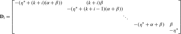 \begin{align*}\textbf{D}_i&=\begin{bmatrix}-(\eta^* + (k+i)(\alpha + \beta)) &\quad (k+i)\beta & & &\\ & \quad -(\eta^*+ (k+i-1)(\alpha + \beta)) & & &\\ & & \ddots &&\\ &&&\quad -(\eta^*+ \alpha+\beta)&\beta\\ &&&&\quad -\eta^*\end{bmatrix}\end{align*}
and
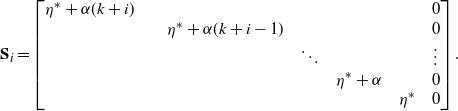 \begin{align*}\textbf{S}_i&=\begin{bmatrix}\eta^* + \alpha(k+i)\quad & & & & & \quad 0\\ & \quad\eta^* + \alpha(k+i-1) & & && \quad 0\\ & & \quad\ddots &&& \quad\vdots\\ &&&\quad\eta^* + \alpha&& \quad 0\\ &&&&\quad\eta^* &\quad 0\end{bmatrix}.\end{align*}
Further, let $\textbf{Z}_n \in \mathbb{R}^{\hat d_n \times \hat d_n}$
for
$\textbf{Z}_n \in \mathbb{R}^{\hat d_n \times \hat d_n}$
for $\hat d_n = \frac{n(n+1)}{2} + (n+1)(k+1)$
be a matrix such that
$\hat d_n = \frac{n(n+1)}{2} + (n+1)(k+1)$
be a matrix such that
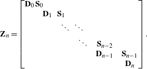 \begin{align*}\textbf{Z}_n=\begin{bmatrix}\textbf{D}_0 & \textbf{S}_0\quad &&&&\\&\quad \textbf{D}_1 & \textbf{S}_1 &&&\\&&\quad \ddots & \ddots &&\\&&& \quad\ddots & \quad \textbf{S}_{n-2} &\\&&&&\quad \textbf{D}_{n-1} & \quad \textbf{S}_{n-1}\\&&&&&\quad \textbf{D}_n\end{bmatrix}.\end{align*}
Then the probability that $N_t = n$
is given by
$N_t = n$
is given by
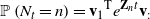 \begin{align}\mathbb{P}\left( N_t = n \right)={{\textbf{v}}_{{1}}}^{\textrm{T}} e^{\textbf{Z}_n t} {{\textbf{v}}_{{:}}}\end{align}
where ${{\textbf{v}}_{{j}}} \in \mathbb{R}^{\hat d_n}$
is the unit column vector for the jth coordinate, and
${{\textbf{v}}_{{j}}} \in \mathbb{R}^{\hat d_n}$
is the unit column vector for the jth coordinate, and ${{\textbf{v}}_{{:}}} = \sum_{j = 0}^{k+n} {{\textbf{v}}_{{\hat d_n - j}}}$
.
${{\textbf{v}}_{{:}}} = \sum_{j = 0}^{k+n} {{\textbf{v}}_{{\hat d_n - j}}}$
.
Proof. This follows directly from viewing $\textbf{Z}_n$
as a sub-matrix of the generator matrix of a continuous-time Markov chain, much as one can do to calculate probabilities of phase-type distributions. Specifically, the sub-generator matrix is defined on the state space
$\textbf{Z}_n$
as a sub-matrix of the generator matrix of a continuous-time Markov chain, much as one can do to calculate probabilities of phase-type distributions. Specifically, the sub-generator matrix is defined on the state space $\mathcal{S} = \bigcup_{i=0}^n \{(0,i), (1,i), \dots, (k+i-1,i),(k+i,i)\}$
. In this scenario, the state
$\mathcal{S} = \bigcup_{i=0}^n \{(0,i), (1,i), \dots, (k+i-1,i),(k+i,i)\}$
. In this scenario, the state $(s_1, s_2)$
represents having
$(s_1, s_2)$
represents having $s_1$
entities in system and having seen
$s_1$
entities in system and having seen $s_2$
arrivals since time 0. Then,
$s_2$
arrivals since time 0. Then, $\textbf{D}_i$
is the sub-generator matrix for transitions among the sub-state space
$\textbf{D}_i$
is the sub-generator matrix for transitions among the sub-state space $\{(k+i,i), (k+i-1,i), \dots, (1,i),(0,i)\}$
to itself (where the states are ordered in that fashion). Similarly,
$\{(k+i,i), (k+i-1,i), \dots, (1,i),(0,i)\}$
to itself (where the states are ordered in that fashion). Similarly, $\textbf{S}_i$
is for transitions from states in
$\textbf{S}_i$
is for transitions from states in $\{(k+i,i), (k+i-1,i), \dots, (1,i),(0,i)\}$
to states in
$\{(k+i,i), (k+i-1,i), \dots, (1,i),(0,i)\}$
to states in $\{(k+i+1, i+1), (k+i,i+1), \dots, (1,i+1),(0,i+1)\}$
. One can then consider this from an absorbing continuous-time Markov chain perspective, since if
$\{(k+i+1, i+1), (k+i,i+1), \dots, (1,i+1),(0,i+1)\}$
. One can then consider this from an absorbing continuous-time Markov chain perspective, since if $n+1$
arrivals occur it is not possible to transition back to any state in which n arrivals had occurred. Hence, we only need to use the matrix
$n+1$
arrivals occur it is not possible to transition back to any state in which n arrivals had occurred. Hence, we only need to use the matrix $\textbf{Z}_n$
to consider up to n arrivals. Then,
$\textbf{Z}_n$
to consider up to n arrivals. Then, $e^{\textbf{Z}_n t}$
is the sub-matrix for probabilities of transitions among states in
$e^{\textbf{Z}_n t}$
is the sub-matrix for probabilities of transitions among states in $\mathcal{S}$
, where the rows will sum to less than 1 as it is possible that the chain has experienced more than n arrivals by time t. Finally, because
$\mathcal{S}$
, where the rows will sum to less than 1 as it is possible that the chain has experienced more than n arrivals by time t. Finally, because $Q_0 = k$
we know that the chain starts in state (k,0); further, because we are seeking the probability that there have been exactly n arrivals by time t, we want the probability of transitions from (k, 0) to any of the states in
$Q_0 = k$
we know that the chain starts in state (k,0); further, because we are seeking the probability that there have been exactly n arrivals by time t, we want the probability of transitions from (k, 0) to any of the states in $\{(k+n,n), (k+n-1,n), \dots, (1,n),(0,n)\}$
.
$\{(k+n,n), (k+n-1,n), \dots, (1,n),(0,n)\}$
.
With these fundamental quantities in hand, let us now turn to explore more nuanced connections between the ESEP and other stochastic processes in the following section. Doing so will provide further comparison between the Hawkes process and the ESEP, and moreover will formally connect the notion of self-excitement to similar concepts such as contagion, virality, and rich-get-richer effects.
3. Relating ephemeral self-excitement to branching processes, random walks, and epidemics
Aside from the original definition, the most frequently utilized result for Hawkes processes is perhaps the immigration–birth representation first shown in [Reference Hawkes and Oakes37]. By viewing a portion of arrivals as immigrants—externally driven and stemming from a homogeneous Poisson process—and then viewing the remaining portion as offspring—excitation-driven descendants of the immigrants and the prior offspring—one can take new perspectives on self-exciting processes. From this position, if an arrival is a descendant then it has a unique parent, the excitement of which spurred this arrival into existence. Every entity has the potential to generate offspring. This viewpoint takes on added meaning in the context of ephemeral self-excitement, as an entity only has the opportunity to generate descendants so long as it remains in the system. In this section, we will use this idea to connect self-exciting processes to well-known stochastic models that have applications ranging from public health to Bayesian statistics. Furthermore, these connections will also help us form comparisons between the Hawkes process and the model we have introduced, the ESEP. The different dynamics are at the forefront of this process comparison, as the branching structure is dictated by the self-excitation caused by a single arrival. For the Hawkes process, this increase in the arrival rate is eternal but ever-diminishing, whereas in the ESEP the jump is ephemeral but constant when it does exist.
3.1. Discrete-time perspectives through branching processes
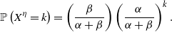
Let us first view these processes through a discrete-time lens as branching processes. In this subsection we will interpret classical branching process results in application to these self-exciting processes. Taking the immigration–birth representation as inspiration, we start by considering the distribution of the total number of offspring of a single arrival. That is, we want to calculate the probability mass function for the number of arrivals that are generated directly from the excitement caused by the initial arrival. To constitute the total number of offspring, we will consider all the children of this initial entity across all time. For the ESEP, this equals the number of arrivals generated by the entity throughout its duration in the system; in the Hawkes process this counts the number of arrivals spurred by the entity as time goes to infinity. Given that the stability conditions are satisfied throughout, in Proposition 5 we calculate these distributions by way of inhomogeneous Poisson processes, yielding a Poisson mixture form for each.
Proposition 5. Let $\beta > \alpha > 0$
. Let
$\beta > \alpha > 0$
. Let $X^\eta$
be the number of new arrivals generated by the excitement caused by an arbitrary initial arrival throughout its duration in the system in an ESEP with jump size
$X^\eta$
be the number of new arrivals generated by the excitement caused by an arbitrary initial arrival throughout its duration in the system in an ESEP with jump size $\alpha$
and expiration rate
$\alpha$
and expiration rate $\beta$
. Then this offspring distribution is geometrically distributed with probability mass function
$\beta$
. Then this offspring distribution is geometrically distributed with probability mass function
 \begin{align}\mathbb{P}\left( X^\eta = k \right) &= \left(\frac{\beta}{\alpha+\beta}\right)\left(\frac{\alpha}{\alpha+\beta}\right)^k.\end{align}
Similarly, let $X^\lambda$
be the number of new arrivals generated by the excitement caused by an arbitrary initial arrival in a Hawkes process with jump size
$X^\lambda$
be the number of new arrivals generated by the excitement caused by an arbitrary initial arrival in a Hawkes process with jump size $\alpha$
and decay rate
$\alpha$
and decay rate $\beta$
. This offspring distribution is then Poisson distributed with probability mass function
$\beta$
. This offspring distribution is then Poisson distributed with probability mass function
 \begin{align}\mathbb{P}\left( X^\lambda = k \right) &= \frac{e^{-\frac{\alpha}\beta}}{k!}\left(\frac{\alpha}\beta\right)^k,\end{align}
where all $k \in \mathbb{N}$
.
$k \in \mathbb{N}$
.
Proof. Without loss of generality, we assume that the initial arrival in each process occurred at time 0. Then, at time $t \geq 0$
, the excitement generated by these initial arrivals has intensities given by
$t \geq 0$
, the excitement generated by these initial arrivals has intensities given by $\alpha e^{-\beta t}$
and
$\alpha e^{-\beta t}$
and $\alpha \textbf{1}\{t < S\}$
for the Hawkes and ESEP processes, respectively, where
$\alpha \textbf{1}\{t < S\}$
for the Hawkes and ESEP processes, respectively, where $S \sim \textrm{Exp}(\beta)$
. Using [Reference Daley and Vere-Jones16], one can note that the offspring distributions across all time can then be expressed as
$S \sim \textrm{Exp}(\beta)$
. Using [Reference Daley and Vere-Jones16], one can note that the offspring distributions across all time can then be expressed as
 \begin{align*}X^\lambda \sim \textrm{Pois}\left(\alpha \int_0^\infty e^{-\beta t} \textrm{d}t\right)\qquad \text{and}\qquad X^\eta \sim \textrm{Pois}\left(\alpha \int_0^\infty \textbf{1}\{t < S\} \textrm{d}t\right),\end{align*}
which are equivalently stated as $X^\lambda \sim \textrm{Pois}\left(\alpha/\beta\right)$
and
$X^\lambda \sim \textrm{Pois}\left(\alpha/\beta\right)$
and $X^\eta \sim \textrm{Pois}\left(\alpha S\right)$
. This now immediately yields the stated distributions for
$X^\eta \sim \textrm{Pois}\left(\alpha S\right)$
. This now immediately yields the stated distributions for $X^\lambda$
and
$X^\lambda$
and $X^\eta$
, as the Poisson–exponential mixture is known to yield a geometric distribution; see for example the overview of Poisson mixtures in [Reference Karlis and Xekalaki39].
$X^\eta$
, as the Poisson–exponential mixture is known to yield a geometric distribution; see for example the overview of Poisson mixtures in [Reference Karlis and Xekalaki39].
We now move towards considering the total progeny of an initial arrival, meaning the total number of arrivals generated by the excitement of an initial arrival and the excitement of its offspring, and of their offspring, and so on across all time. It is important to note that in contrast to the number of offspring, the progeny includes the initial arrival itself. As we will see, the stability of the self-exciting processes implies that this total number of descendants is almost surely finite. This demonstrates the necessity of immigration for these processes to survive. From the offspring distributions in Proposition 5, the Hawkes descendant process is a Poisson branching process, and similarly the ESEP is a geometric branching process. These are well-studied models in branching processes, so we have many results available to us. In fact, we now use a result for random walks with potentially multiple simultaneous steps forward to derive the progeny distributions for these two processes. This is through the well-known hitting time theorem, stated below in Lemma 1.
Lemma 1. (Hitting time theorem.) The total progeny Z of a branching process with descendant distribution equivalent to $X_1$
is
$X_1$
is
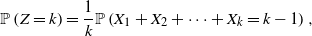 \begin{align*}\mathbb{P}\left( Z = k \right) = \frac{1}{k}\mathbb{P}\left( X_1 + X_2 + \dots + X_k = k -1 \right),\end{align*}
where $X_1, \dots, X_k$
are i.i.d. for all
$X_1, \dots, X_k$
are i.i.d. for all $k \in \mathbb{Z}^+$
.
$k \in \mathbb{Z}^+$
.
Proof. See [Reference Otter52] for the original statement and proof in terms of random walks; a review and elementary proof are given in the brief note [Reference Van der Hofstad and Keane58].
We now use the hitting time theorem to give the progeny distributions for the Hawkes process and the ESEP in Proposition 6. This is a common technique for branching processes, and it now yields valuable insight into these two self-exciting models.
Proposition 6. Let $\beta > \alpha > 0$
. Let
$\beta > \alpha > 0$
. Let $Z^\eta$
be a random variable for the total progeny of an arbitrary arrival in an ESEP with intensity jump
$Z^\eta$
be a random variable for the total progeny of an arbitrary arrival in an ESEP with intensity jump $\alpha$
and expiration rate
$\alpha$
and expiration rate $\beta$
. Likewise, let
$\beta$
. Likewise, let $Z^\lambda$
be a random variable for the total progeny of an arbitrary arrival in a Hawkes process with intensity jump
$Z^\lambda$
be a random variable for the total progeny of an arbitrary arrival in a Hawkes process with intensity jump $\alpha$
and decay rate
$\alpha$
and decay rate $\beta$
. Then the probability mass functions for
$\beta$
. Then the probability mass functions for $Z^\eta$
and
$Z^\eta$
and $Z^\lambda$
are given by
$Z^\lambda$
are given by
 \begin{align}&\mathbb{P}\left( Z^\eta = k \right)=\frac{1}{k} \left(\begin{array}{c}2k-2\\k-1\end{array}\right) \left(\frac{\beta}{\beta + \alpha}\right)^k\left(\frac{\alpha}{\beta + \alpha}\right)^{k-1}\text{and}&\mathbb{P}\left( Z^\lambda = k \right)=\frac{e^{-\frac{\alpha}{\beta} k}}{k!}\left(\frac{\alpha k}{\beta}\right)^{k-1},\end{align}
where $k \in \mathbb{Z}^+$
.
$k \in \mathbb{Z}^+$
.
Proof. This follows from applying Lemma 1 to Proposition 5. Because the sum of independent Poisson random variables is Poisson distributed with the sum of the rates, we have that
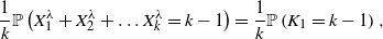 \begin{align*}\frac{1}{k}\mathbb{P}\left( X^\lambda_{1} + X^\lambda_{2} + \dots X^\lambda_{k} = k -1 \right)=\frac{1}k \mathbb{P}\left( K_1 = k -1 \right),\end{align*}
where $K_1 \sim \textrm{Pois}\left(\frac{\alpha k}{\beta}\right)$
. This now yields the expression for the probability mass function for
$K_1 \sim \textrm{Pois}\left(\frac{\alpha k}{\beta}\right)$
. This now yields the expression for the probability mass function for $Z^\lambda$
. Similarly for
$Z^\lambda$
. Similarly for $Z_\eta$
we note that the sum of independent geometric random variables has a negative binomial distribution, which implies that
$Z_\eta$
we note that the sum of independent geometric random variables has a negative binomial distribution, which implies that
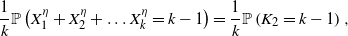 \begin{align*}\frac{1}{k}\mathbb{P}\left( X^\eta_{1} + X^\eta_{2} + \dots X^\eta_{k} = k -1 \right)=\frac{1}k \mathbb{P}\left( K_2 = k -1 \right),\end{align*}
where $K_2 \sim \textrm{NegBin}\left(k,\frac{\alpha}{\beta + \alpha}\right)$
, and this completes the proof.
$K_2 \sim \textrm{NegBin}\left(k,\frac{\alpha}{\beta + \alpha}\right)$
, and this completes the proof.
For a visual comparison of the descendants in the ESEP and the Hawkes process, we plot these two progeny distributions for equivalent parameters in Figure 2. As suggested by the variance ordering in Proposition 2, the tail of the ESEP progeny distribution is heavier than that of the Hawkes process.
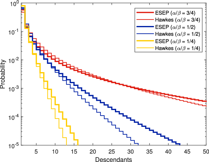
Figure 2. Progeny distributions for the ESEP and the Hawkes process with matching parameters.
We can note that while one can calculate the mean of each progeny distribution via the probability mass functions in Proposition 6, it can also easily be found using Wald’s identity. Through standard infinitesimal generator approaches, one can calculate that the expected number of arrivals (including by immigration) in the ESEP is
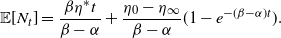 \begin{align*}{\mathbb{E}\!\left[N_t\right]} = \frac{\beta \eta^* t}{\beta - \alpha} + \frac{\eta_0 - \eta_\infty}{\beta - \alpha}(1-e^{-(\beta - \alpha)t}).\end{align*}
However, using these branching process representations, we can also express this as
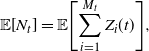 \begin{align*}{\mathbb{E}\!\left[N_t\right]} = {\mathbb{E}\!\left[\sum_{i=1}^{M_t} Z_{i}(t)\right]},\end{align*}
where $M_t$
is a Poisson process with rate
$M_t$
is a Poisson process with rate $\eta^*$
and
$\eta^*$
and $Z_i(t)$
are the total progeny up to time
$Z_i(t)$
are the total progeny up to time $t \geq 0$
that are descended from the ith immigrant arrival. Now, by applying Wald’s identity to the limit of
$t \geq 0$
that are descended from the ith immigrant arrival. Now, by applying Wald’s identity to the limit of $\frac{1}{t}{\mathbb{E}\!\left[N_t\right]}$
as
$\frac{1}{t}{\mathbb{E}\!\left[N_t\right]}$
as $t \to \infty$
, we see that
$t \to \infty$
, we see that
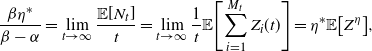 \begin{align*}\frac{\beta \eta^* }{\beta - \alpha} = \lim_{t \to \infty} \frac{{\mathbb{E}\!\left[N_t\right]}}{t} = \lim_{t\to\infty}\frac{1}{t}{\mathbb{E}\!\left[\sum_{i=1}^{M_t} Z_{i}(t)\right]} = \eta^* {\mathbb{E}\!\left[Z^\eta\right]} ,\end{align*}
and so ${\mathbb{E}\!\left[Z^\eta\right]} = \frac{\beta}{\beta - \alpha}$
. By analogous arguments for the Hawkes process, we see that
${\mathbb{E}\!\left[Z^\eta\right]} = \frac{\beta}{\beta - \alpha}$
. By analogous arguments for the Hawkes process, we see that ${\mathbb{E}\!\left[Z^\lambda\right]} = \frac{\beta}{\beta-\alpha}$
.
${\mathbb{E}\!\left[Z^\lambda\right]} = \frac{\beta}{\beta-\alpha}$
.
As a final branching process comparison between these two processes, we calculate the distribution of the total number of generations of descendants of an initial arrival in the ESEP and the Hawkes process. That is, let the first entity be the first generation, its offspring the second generation, their offspring the third, and so on. In Proposition 7 we find the probability mass function for the ESEP in closed form and a recurrence relation for the cumulative distribution function for the Hawkes process.
Proposition 7. Let $\beta > \alpha > 0$
. Let
$\beta > \alpha > 0$
. Let $\mathcal{G}^\eta$
be the number of distinct arrival generations across the full progeny of an initial arrival in an ESEP with intensity jump
$\mathcal{G}^\eta$
be the number of distinct arrival generations across the full progeny of an initial arrival in an ESEP with intensity jump $\alpha$
and service rate
$\alpha$
and service rate $\beta$
. Then the probability mass function for
$\beta$
. Then the probability mass function for $\mathcal{G}^\eta$
is given by
$\mathcal{G}^\eta$
is given by
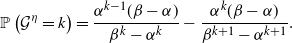 \begin{align}\mathbb{P}\left( \mathcal{G}^\eta = k \right)=\frac{\alpha^{k-1}(\beta-\alpha)}{\beta^k-\alpha^k}-\frac{\alpha^k(\beta-\alpha)}{\beta^{k+1} - \alpha^{k+1}}.\end{align}
Likewise, let $\mathcal{G}^\lambda$
be the number of distinct arrival generations in the full progeny of an initial arrival for a Hawkes process with intensity jump
$\mathcal{G}^\lambda$
be the number of distinct arrival generations in the full progeny of an initial arrival for a Hawkes process with intensity jump $\alpha > 0$
and decay rate
$\alpha > 0$
and decay rate $\beta$
. Then
$\beta$
. Then $\mathcal{G}^\lambda$
has cumulative distribution function
$\mathcal{G}^\lambda$
has cumulative distribution function $F_{\mathcal{G^\lambda}}(k) = \mathbb{P}\left( \mathcal{G}^\lambda \leq k \right)$
satisfying the recursion
$F_{\mathcal{G^\lambda}}(k) = \mathbb{P}\left( \mathcal{G}^\lambda \leq k \right)$
satisfying the recursion
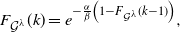 \begin{align}F_{\mathcal{G^\lambda}}(k) = e^{-\frac{\alpha}{\beta}\left(1 - F_{\mathcal{G^\lambda}}(k-1)\right)} ,\end{align}
where $F_{\mathcal{G^\lambda}}(0) = 0$
and all
$F_{\mathcal{G^\lambda}}(0) = 0$
and all $k \in \mathbb{Z}^+$
.
$k \in \mathbb{Z}^+$
.
Proof. Let $Y_k^\lambda$
and
$Y_k^\lambda$
and $Y_k^\eta$
be Galton–Watson branching processes defined as
$Y_k^\eta$
be Galton–Watson branching processes defined as
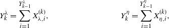 \begin{align}&Y_k^\lambda = \sum_{i=1}^{Y_{k-1}^\lambda} X_{\lambda, i}^{(k)},&Y_k^\eta = \sum_{i=1}^{Y_{k-1}^\eta} X_{\eta, i}^{(k)},\end{align}
with $X_{\lambda, i}^{(k)} \stackrel{i.i.d.}{\sim} \textrm{Pois}\left(\frac{\alpha}{\beta}\right)$
,
$X_{\lambda, i}^{(k)} \stackrel{i.i.d.}{\sim} \textrm{Pois}\left(\frac{\alpha}{\beta}\right)$
, $X_{\eta, i}^{(k)} \stackrel{i.i.d.}{\sim} \textrm{Geo}\left(\frac{\alpha}{\alpha+\beta}\right)$
, and
$X_{\eta, i}^{(k)} \stackrel{i.i.d.}{\sim} \textrm{Geo}\left(\frac{\alpha}{\alpha+\beta}\right)$
, and $Y_0^\lambda = Y_0^\eta = 1$
. These processes then have probability generating functions
$Y_0^\lambda = Y_0^\eta = 1$
. These processes then have probability generating functions
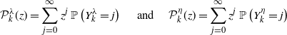 \begin{align*}\mathcal{P}_k^\lambda(z)=\sum_{j=0}^\infty z^j\, \mathbb{P}\left( Y_k^\lambda = j \right)\quad\text{ and }\quad\mathcal{P}_k^\eta(z)=\sum_{j=0}^\infty z^j\, \mathbb{P}\left( Y_k^\eta = j \right)\end{align*}
that are given by the recursions $\mathcal{P}_{k+1}^\lambda(z) = \mathcal{P}_{X^\lambda}\left(\mathcal{P}_{k}^\lambda(z)\right)$
and
$\mathcal{P}_{k+1}^\lambda(z) = \mathcal{P}_{X^\lambda}\left(\mathcal{P}_{k}^\lambda(z)\right)$
and $\mathcal{P}_{k+1}^\lambda(z) = \mathcal{P}_{X^\eta}\left(\mathcal{P}_{k}^\eta(z)\right)$
with
$\mathcal{P}_{k+1}^\lambda(z) = \mathcal{P}_{X^\eta}\left(\mathcal{P}_{k}^\eta(z)\right)$
with $\mathcal{P}_{1}^\lambda(z) = \mathcal{P}_{X^\lambda}(z)$
and
$\mathcal{P}_{1}^\lambda(z) = \mathcal{P}_{X^\lambda}(z)$
and $\mathcal{P}_{1}^\eta(z) = \mathcal{P}_{X^\eta}(z)$
, where
$\mathcal{P}_{1}^\eta(z) = \mathcal{P}_{X^\eta}(z)$
, where $\mathcal{P}_{X^\lambda}(z)$
and
$\mathcal{P}_{X^\lambda}(z)$
and $\mathcal{P}_{X^\eta}(z)$
are the probability generating functions of
$\mathcal{P}_{X^\eta}(z)$
are the probability generating functions of $X_{\lambda,1}^{(1)}$
and
$X_{\lambda,1}^{(1)}$
and $X_{\eta,1}^{(1)}$
, respectively; see e.g. Section XII.5 of [Reference Feller27]. One can then use induction to observe that
$X_{\eta,1}^{(1)}$
, respectively; see e.g. Section XII.5 of [Reference Feller27]. One can then use induction to observe that
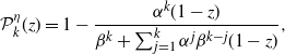 \begin{align*}\mathcal{P}_k^\eta(z)=1 - \frac{\alpha^k(1-z)}{\beta^k + \sum_{j=1}^k\alpha^j \beta^{k-j}(1-z)},\end{align*}
whereas $\mathcal{P}_k^\lambda(z) = e^{-\frac{\alpha}{\beta}\left(1 - \mathcal{P}^\lambda_{k-1}(z)\right)}$
, with
$\mathcal{P}_k^\lambda(z) = e^{-\frac{\alpha}{\beta}\left(1 - \mathcal{P}^\lambda_{k-1}(z)\right)}$
, with $\mathcal{P}^\lambda_1(z) = e^{-\frac{\alpha}{\beta}(1-z)}$
. Because of their shared offspring distribution constructions, the number of the progeny in the kth arrival generations of the Hawkes process and the ESEP are equivalent in distribution to
$\mathcal{P}^\lambda_1(z) = e^{-\frac{\alpha}{\beta}(1-z)}$
. Because of their shared offspring distribution constructions, the number of the progeny in the kth arrival generations of the Hawkes process and the ESEP are equivalent in distribution to $Y_k^\lambda$
and
$Y_k^\lambda$
and $Y_k^\eta$
, respectively. In this way, we can express
$Y_k^\eta$
, respectively. In this way, we can express $\mathcal{G}^\lambda$
and
$\mathcal{G}^\lambda$
and $\mathcal{G}^\eta$
as
$\mathcal{G}^\eta$
as
 \begin{align*}\mathcal{G}^\lambda=\inf\{ k \in \mathbb{Z}^+ \mid Y_k^\lambda = 0 \}\quad\text{ and }\quad\mathcal{G}^\eta=\inf\{ k \in \mathbb{Z}^+ \mid Y_k^\eta = 0 \}.\end{align*}
This leads us to observe that the events $\{\mathcal{G}^\lambda = j\}$
and
$\{\mathcal{G}^\lambda = j\}$
and $\{Y_j^\lambda = 0, Y_{j-1}^\lambda > 0\}$
are equivalent, as are
$\{Y_j^\lambda = 0, Y_{j-1}^\lambda > 0\}$
are equivalent, as are $\{\mathcal{G}^\eta = j\}$
and
$\{\mathcal{G}^\eta = j\}$
and $\{Y_j^\eta = 0, Y_{j-1}^\eta > 0\}$
. Focusing for now on
$\{Y_j^\eta = 0, Y_{j-1}^\eta > 0\}$
. Focusing for now on $\mathcal{G}^\lambda$
, we have that
$\mathcal{G}^\lambda$
, we have that
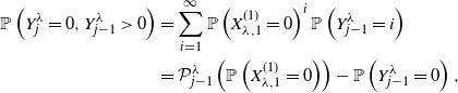 \begin{align*}\mathbb{P}\left( Y_j^\lambda = 0, Y_{j-1}^\lambda > 0 \right)&=\sum_{i=1}^\infty \mathbb{P}\left( X_{\lambda,1}^{(1)} = 0 \right)^i\mathbb{P}\left( Y_{j-1}^\lambda = i \right)\\&=\mathcal{P}^\lambda_{j-1}\left(\mathbb{P}\left( X_{\lambda,1}^{(1)} = 0 \right)\right)-\mathbb{P}\left( Y_{j-1}^\lambda = 0 \right),\end{align*}
and since $\mathbb{P}\left( K = 0 \right) = \mathcal{P}(0)$
for any nonnegative discrete random variable K with probability generating function
$\mathbb{P}\left( K = 0 \right) = \mathcal{P}(0)$
for any nonnegative discrete random variable K with probability generating function $\mathcal{P}(z)$
, this yields
$\mathcal{P}(z)$
, this yields
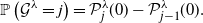 \begin{align*}\mathbb{P}\left( \mathcal{G}^\lambda = j \right) = \mathcal{P}^\lambda_{j}(0) - \mathcal{P}^\lambda_{j-1}(0) .\end{align*}
Using $\mathcal{P}^\lambda_{0}(0) = 0$
, this telescoping sum now produces the stated form of the cumulative distribution function for
$\mathcal{P}^\lambda_{0}(0) = 0$
, this telescoping sum now produces the stated form of the cumulative distribution function for $\mathcal{G}^\lambda$
. By analogous arguments for
$\mathcal{G}^\lambda$
. By analogous arguments for $\mathcal{G}^\eta$
, we complete the proof.
$\mathcal{G}^\eta$
, we complete the proof.
In the following subsection we focus on the ESEP, using the insight we have now gained from branching processes to connect this process to stochastic models for preferential attachment that are popular in the Bayesian nonparametric and machine learning literatures.
3.2. Similarities with preferential attachment and Bayesian statistics models
In the branching process perspective of the ESEP, consider the total number of active families at one point in time. That is, across all the entities present in the system at a given time, we are interested in the number of distinct families to which these entities belong. As each arrival occurs, the new entity either belongs to one of the existing families, meaning that the entity is a descendant, or it forms a new family, which is to say that it is an immigrant. If the entity is joining an existing family, it is more likely to join families that have more presently active family members.
We can note that these dynamics are quite similar to the definition of the Chinese restaurant process (CRP); see Chapter 11 in [Reference Aldous3]. The CRP models the successive arrivals of customers to a restaurant with infinitely many tables that each have infinitely many seats. Each arriving customer chooses which table to join based on the decisions of those before. Specifically, the nth customer to arrive joins table i with probability $\frac{c_i}{n-1+\lambda}$
or otherwise starts a new table with probability
$\frac{c_i}{n-1+\lambda}$
or otherwise starts a new table with probability $\frac{\lambda}{n-1+\lambda}$
, where
$\frac{\lambda}{n-1+\lambda}$
, where $c_i$
is the number of customers at table i and
$c_i$
is the number of customers at table i and $\lambda > 0$
. As the number seated at table i grows larger, it is increasingly likely that the next customer will choose to sit at table i. In the ESEP, a new arrival at time
$\lambda > 0$
. As the number seated at table i grows larger, it is increasingly likely that the next customer will choose to sit at table i. In the ESEP, a new arrival at time $t \geq 0$
is generated as part of active excitement family i with probability
$t \geq 0$
is generated as part of active excitement family i with probability $\frac{\alpha Q_{t,i}}{\alpha Q_t + \eta^*}$
and otherwise is an externally generated arrival with probability
$\frac{\alpha Q_{t,i}}{\alpha Q_t + \eta^*}$
and otherwise is an externally generated arrival with probability $\frac{\eta^*}{\alpha Q_t + \eta^*}$
, where
$\frac{\eta^*}{\alpha Q_t + \eta^*}$
, where $Q_{t,i}$
is the number of active exciters in the system at time t in the ith excitement family with
$Q_{t,i}$
is the number of active exciters in the system at time t in the ith excitement family with $Q_t = \sum_{i} Q_{t,i}$
. By normalizing the numerator and denominator of these probabilities by
$Q_t = \sum_{i} Q_{t,i}$
. By normalizing the numerator and denominator of these probabilities by $\frac{1}\alpha$
, we see that these dynamics match the CRP almost exactly. The difference is hardly a novel idea for restaurants—in the ESEP diners eventually leave. This departure then decreases the number of customers at the table, making it less attractive to the next person to arrive.
$\frac{1}\alpha$
, we see that these dynamics match the CRP almost exactly. The difference is hardly a novel idea for restaurants—in the ESEP diners eventually leave. This departure then decreases the number of customers at the table, making it less attractive to the next person to arrive.
In addition to being an intriguing stochastic model, the CRP is also of interest for Bayesian statistics and machine learning through its connection to Bayesian nonparametric mixture models, specifically Dirichlet process mixtures. By consequence, the CRP then also has commonality with urn models and models for preferential attachment; see e.g. [Reference Blackwell and MacQueen10]. The CRP is also established enough to have its own generalizations, such as the distance-dependent CRP in [Reference Blei and Frazier12], in which the probability that a customer joins a table is dependent on a distance metric, and the recurrent CRP in [Reference Ahmed and Xing1], in which the restaurant closes at the end of each day, forcing all of that day’s customers to simultaneously depart. Drawing inspiration from the CRP and from the branching process perspectives of the ESEP, we investigate the distribution of the number of active families in the ESEP. This is equivalently stated as the number of active tables in a continuous-time CRP in which customers leave after their exponentially distributed meal durations. To begin, we first find the expected amount of time until a newly formed table becomes empty.
Proposition 8. Suppose that an ESEP receives an initial arrival at time 0. Let $X_t$
be the number of entities in the system at time
$X_t$
be the number of entities in the system at time $t \geq 0$
that are progeny of the initial arrival, and let
$t \geq 0$
that are progeny of the initial arrival, and let $\tau$
be a stopping time such that
$\tau$
be a stopping time such that $\tau = \inf \{t \geq 0 \mid X_t = 0\}$
. Then the expected value of
$\tau = \inf \{t \geq 0 \mid X_t = 0\}$
. Then the expected value of $\tau$
is
$\tau$
is
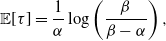 \begin{align}{\mathbb{E}\!\left[\tau\right]}=\frac{1}{\alpha}\log\left(\frac{\beta}{\beta - \alpha}\right),\end{align}
where $\alpha > 0$
is the intensity jump size and
$\alpha > 0$
is the intensity jump size and $\beta > \alpha$
is the expiration rate.
$\beta > \alpha$
is the expiration rate.
Proof. To observe this, we note that $X_t$
can be viewed as the state of an absorbing continuous-time Markov chain on the nonnegative integers. State 0 is the single absorbing state; in any other state j, the two possible transitions are to
$X_t$
can be viewed as the state of an absorbing continuous-time Markov chain on the nonnegative integers. State 0 is the single absorbing state; in any other state j, the two possible transitions are to $j+1$
at rate
$j+1$
at rate $\alpha j$
and to
$\alpha j$
and to $j-1$
at rate
$j-1$
at rate $\mu j$
, as visualized below.
$\mu j$
, as visualized below.
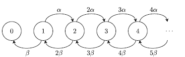
Then, $\tau$
is the time of absorption into state 0 when starting in state 1, and so
$\tau$
is the time of absorption into state 0 when starting in state 1, and so ${\mathbb{E}\!\left[\tau\right]}$
can be calculated by standard first-step analysis approaches, yielding
${\mathbb{E}\!\left[\tau\right]}$
can be calculated by standard first-step analysis approaches, yielding
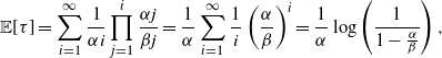 \begin{align*}{\mathbb{E}\!\left[\tau\right]}=\sum_{i=1}^\infty \frac{1}{\alpha i} \prod_{j=1}^{i} \frac{\alpha j}{\beta j} = \frac{1}{\alpha}\sum_{i=1}^\infty \frac{1}{i}\left(\frac{\alpha}{\beta}\right)^i = \frac{1}{\alpha}\log\left(\frac{1}{1-\frac{\alpha}{\beta}}\right),\end{align*}
and this simplifies to the stated result.
Proposition 8 gives the expectation of the total time an excitement family is active in the system. Using this, in Proposition 9 we now employ a classical queueing theory result to find the exact distribution of the number of active families simultaneously in the system in steady state.
Proposition 9. Let B be the number of distinct excitement families that have progeny active in the system in steady state of an ESEP with baseline intensity $\eta^* > 0$
, intensity jump
$\eta^* > 0$
, intensity jump $\alpha > 0$
, and expiration rate
$\alpha > 0$
, and expiration rate $\beta > \alpha$
. Then
$\beta > \alpha$
. Then $B \sim \textrm{Pois}\left(\frac{\eta^*}{\alpha}\log \left(\frac{\beta}{\beta - \alpha}\right)\right)$
.
$B \sim \textrm{Pois}\left(\frac{\eta^*}{\alpha}\log \left(\frac{\beta}{\beta - \alpha}\right)\right)$
.
Proof. We first note that new excitement families are started when a baseline-generated arrival occurs, which follows a Poisson process with rate $\nu^*$
. The duration of the excitement family’s time in system then has mean given by Proposition 8. Because there is no limitation on the number of possible families in the system at once, this is equivalent to an infinite-server queue with Poisson process arrivals and generally distributed service, an M/G/
$\nu^*$
. The duration of the excitement family’s time in system then has mean given by Proposition 8. Because there is no limitation on the number of possible families in the system at once, this is equivalent to an infinite-server queue with Poisson process arrivals and generally distributed service, an M/G/ $\infty$
queue in Kendall notation. This process is known to have Poisson distributed steady-state distribution (see e.g. [Reference Eick, Massey and Whitt23]), with mean given by the product of the arrival rate and the mean service duration, which yields the stated form for B.
$\infty$
queue in Kendall notation. This process is known to have Poisson distributed steady-state distribution (see e.g. [Reference Eick, Massey and Whitt23]), with mean given by the product of the arrival rate and the mean service duration, which yields the stated form for B.
An interesting consequence of the number of active families being Poisson distributed and the total number in system being negative-binomially distributed is that it suggests that the number of simultaneously active family members is logarithmically distributed. We observe this via the known compound Poisson representation of the negative binomial distribution [Reference Willmot60]. For $B \sim \textrm{Pois}\left(\frac{\eta^*}{\alpha}\log \left(\frac{\beta}{\beta - \alpha}\right)\right)$
,
$B \sim \textrm{Pois}\left(\frac{\eta^*}{\alpha}\log \left(\frac{\beta}{\beta - \alpha}\right)\right)$
, $Q \sim \textrm{NegBin}\left(\frac{\alpha}{\beta}, \frac{\eta^*}{\alpha}\right)$
, and
$Q \sim \textrm{NegBin}\left(\frac{\alpha}{\beta}, \frac{\eta^*}{\alpha}\right)$
, and $L_i \stackrel{\textrm{i.i.d.}}{\sim} \textrm{Log}\left(\frac{\alpha}{\beta} \right)$
, one can observe that
$L_i \stackrel{\textrm{i.i.d.}}{\sim} \textrm{Log}\left(\frac{\alpha}{\beta} \right)$
, one can observe that
 \begin{align*}Q \stackrel{D}{=} \sum_{i=1}^B L_i,\end{align*}
where $\mathbb{P}\left( L_1 = k \right) = \left(\frac{\alpha}{\beta}\right)^k\left(k \log\left(\frac{\beta}{\beta-\alpha}\right)\right)^{-1}$
for all
$\mathbb{P}\left( L_1 = k \right) = \left(\frac{\alpha}{\beta}\right)^k\left(k \log\left(\frac{\beta}{\beta-\alpha}\right)\right)^{-1}$
for all $k \in \mathbb{Z}^+$
. Thus, the idea that the number of active members of each family is logarithmically distributed follows from the fact that this is a sum of positive integer-valued random variables, of which there are as many as there are active families, and this sum is equal to the total number in system.
$k \in \mathbb{Z}^+$
. Thus, the idea that the number of active members of each family is logarithmically distributed follows from the fact that this is a sum of positive integer-valued random variables, of which there are as many as there are active families, and this sum is equal to the total number in system.
3.3. Connections to epidemic models
As a final observation regarding the ESEP and its connections to other stochastic models, consider disease spread. As we discussed in the introduction to this paper, when a person becomes sick with a contagious disease she increases the rate of new infections through her contact with others. Furthermore, when a person recovers from a disease such as the flu, she is no longer contagious and thus no longer contributes to the rate of disease spread. While we have discussed in the introduction that this scenario has the hallmarks of self-excitement qualitatively, a classic model for studying this phenomenon is the susceptible–infected–susceptible (SIS) process.
In the SIS model there is a finite population of $N \in \mathbb{Z}^+$
individuals. Each individual takes on one of two states, either infected or susceptible. Let
$N \in \mathbb{Z}^+$
individuals. Each individual takes on one of two states, either infected or susceptible. Let $I_t$
be the number infected at time
$I_t$
be the number infected at time $t \geq 0$
, and let
$t \geq 0$
, and let $S_t$
be the number susceptible. In the continuous-time stochastic SIS model, each infected individual recovers after an exponentially distributed duration of the illness. Once a person recovers from the disease, she becomes susceptible again. Because there is a finite population, the rate of new infections depends on both the number infected and the number susceptible; a new person falls ill at a rate proportional to
$S_t$
be the number susceptible. In the continuous-time stochastic SIS model, each infected individual recovers after an exponentially distributed duration of the illness. Once a person recovers from the disease, she becomes susceptible again. Because there is a finite population, the rate of new infections depends on both the number infected and the number susceptible; a new person falls ill at a rate proportional to $ I_t\cdot \frac{S_t}{N}$
. Because this continuous-time Markov chain would be absorbed into state
$ I_t\cdot \frac{S_t}{N}$
. Because this continuous-time Markov chain would be absorbed into state $I_t = 0$
, it is common to include an exogenous infection rate proportional to just
$I_t = 0$
, it is common to include an exogenous infection rate proportional to just $\frac{S_t}{N}$
. We will refer to this model as the stochastic SIS with exogenous infections; Figure 3 shows the rate diagram for the transitions from infected to susceptible and from susceptible to infected. For the sake of comparison, we set the exogenous infection rate as
$\frac{S_t}{N}$
. We will refer to this model as the stochastic SIS with exogenous infections; Figure 3 shows the rate diagram for the transitions from infected to susceptible and from susceptible to infected. For the sake of comparison, we set the exogenous infection rate as $\eta^*$
, the epidemic infection rate as
$\eta^*$
, the epidemic infection rate as $\alpha$
, and the recovery rate as
$\alpha$
, and the recovery rate as $\beta$
.
$\beta$
.
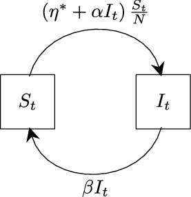
Figure 3. Stochastic SIS model with exogenous infections.
One can note that there are immediate similarities between this process and the ESEP. That is, new infections increase the infection rate while recoveries decrease it, and infections can be the result of either external or internal stimuli. However, the primary difference between these two models is that the SIS process has a finite population, whereas the ESEP does not. In Proposition 10 we find that as this population size grows large the difference between these models fades, yielding that the distribution of the number infected in the exogenously driven SIS model converges to the distribution of the queue length in the ESEP.
Proposition 10. Let $I_t$
be the number of infected individuals at time
$I_t$
be the number of infected individuals at time $t \geq 0$
in an exogenously driven stochastic SIS model with population size
$t \geq 0$
in an exogenously driven stochastic SIS model with population size $N \in \mathbb{Z}^+$
, exogenous infection rate
$N \in \mathbb{Z}^+$
, exogenous infection rate $\eta^* > 0$
, epidemic infection rate
$\eta^* > 0$
, epidemic infection rate $\alpha > 0$
, and recovery rate
$\alpha > 0$
, and recovery rate $\beta > 0$
. Then, as
$\beta > 0$
. Then, as $N \to \infty$
,
$N \to \infty$
,
 \begin{align*}I_t\stackrel{D}{\Longrightarrow}Q_t,\end{align*}
where $Q_t$
is the active number in system at time t for an ESEP with baseline intensity
$Q_t$
is the active number in system at time t for an ESEP with baseline intensity $\eta^*$
, intensity jump
$\eta^*$
, intensity jump $\alpha$
, and expiration rate
$\alpha$
, and expiration rate $\beta$
.
$\beta$
.
Proof. Because the SIS model is a Markov process, one can use the infinitesimal generator approach to find a time derivative for the moment generating function of the number of infected individuals at time $t \geq 0$
. Thus, by noting that
$t \geq 0$
. Thus, by noting that $S_t = N - I_t$
we have that
$S_t = N - I_t$
we have that
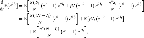 \begin{align*}\frac{\textrm{d}}{\textrm{d}t}{\mathbb{E}\!\left[e^{\theta I_t}\right]}&={\mathbb{E}\!\left[\frac{\alpha I_t S_t}{N} \left( e^{\theta}-1\right) e^{\theta I_t}+\beta I \left(e^{-\theta} - 1 \right) e^{\theta I_t}+\frac{\eta^* S_t}{N} \left(e^{\theta} - 1\right) e^{\theta I_t}\right]}\\&={\mathbb{E}\!\left[\frac{\alpha I_t (N - I_t)}{N} \left( e^{\theta}-1\right) e^{\theta I_t}\right]}+{\mathbb{E}\!\left[\beta I_t \left(e^{-\theta} - 1 \right) e^{\theta I_t}\right]}\\&\qquad +{\mathbb{E}\!\left[\frac{\eta^* (N- I_t)}{N} \left(e^{\theta} - 1\right) e^{\theta I_t}\right]},\end{align*}
which we can re-express in PDE form as
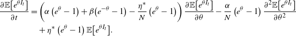 \begin{align*}\frac{\partial {\mathbb{E}\!\left[e^{\theta I_t}\right]}}{\partial t}&=\left(\alpha \left( e^{\theta}-1\right)+\beta\! \left(e^{-\theta} - 1 \right)-\frac{\eta^* }{N} \left(e^{\theta} - 1\right)\right)\frac{\partial {\mathbb{E}\!\left[e^{\theta I_t}\right]}}{\partial \theta}-\frac{\alpha }{N} \left( e^{\theta}-1\right)\frac{\partial^2 {\mathbb{E}\!\left[e^{\theta I_t}\right]}}{\partial \theta^2}\\&\quad+\eta^* \left(e^{\theta} - 1\right){\mathbb{E}\!\left[e^{\theta I_t}\right]}.\end{align*}
Now as the population size $N \to \infty$
, this converges to
$N \to \infty$
, this converges to
 \begin{align*}\frac{\partial {\mathbb{E}\!\left[e^{\theta I_t}\right]}}{\partial t}&=\left(\alpha \left( e^{\theta}-1\right)+\beta\! \left(e^{-\theta} - 1 \right)\right)\frac{\partial {\mathbb{E}\!\left[e^{\theta I_t}\right]}}{\partial \theta}+\eta^* \left(e^{\theta} - 1\right){\mathbb{E}\!\left[e^{\theta I_t}\right]},\end{align*}
which we can recognize as the PDE for the moment generating function of the ESEP through its own infinitesimal generator.
As a demonstration of this convergence, we plot the empirical steady-state distribution of the SIS process for increasing population size below in Figure 4. Note that in this example the distributions appear fairly close for populations of size $N = 1,000$
. On the scale of the populations of cities or even some larger high schools, this is quite small. At a medium university size of
$N = 1,000$
. On the scale of the populations of cities or even some larger high schools, this is quite small. At a medium university size of $N = 10,000$
, the distributions are essentially indistinguishable.
$N = 10,000$
, the distributions are essentially indistinguishable.
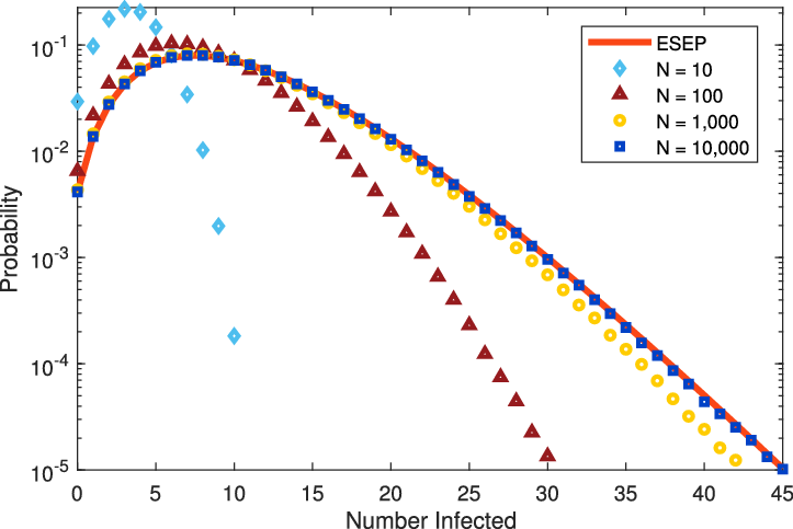
Figure 4. Steady-state distribution of the number infected in the exogenously driven SIS model for increasing population size N, where $\eta^* = 10$
,
$\eta^* = 10$
, $\alpha = 2$
, and
$\alpha = 2$
, and $\beta = 3$
.
$\beta = 3$
.
We would be remiss if we did not note that connections from epidemic models to birth–death processes are not new. For example, [Reference Ball8] demonstrated that epidemic models converge to birth–death processes, and [Reference Singh and Myers56] even noted that the exogenously driven susceptible–infected–recovered (SIR) model—in which people cannot become reinfected—converges to a linear birth–death–immigration process; however, these works did not outright form connections to self-exciting processes. In [Reference Rizoiu54], the similarities between the Hawkes process and the SIR process are shown and formal connections are made, although this is through a generalization of the Hawkes process defined on a finite population rather than through increasing the epidemic model population size. Regardless, these prior works serve to expand the practical relevance of the ESEP, as they show that such epidemic models are also of use outside of public health. For example, these models have been used to study the phenomenon of contagion in areas such as product adoption, idea spread, and social influence. These all also naturally relate to the concept of self-excitement, and in Proposition 10 we observe that this connection can be formalized.
These connections take on added importance in the contemporary context of the COVID-19 public health crisis. It is worth noting that the convergence of distributions in Proposition 10 does not require our commonly assumed stability condition $\beta > \alpha$
. Thus, this convergence also covers potential pandemic scenarios in which
$\beta > \alpha$
. Thus, this convergence also covers potential pandemic scenarios in which $\alpha \geq \beta$
. In such settings, one can quickly observe that the mean number infected by time t is such that
$\alpha \geq \beta$
. In such settings, one can quickly observe that the mean number infected by time t is such that ${\mathbb{E}\!\left[N_t\right]} \in O(e^{(\alpha - \beta)t})$
, reproducing the exponential growth exhibited by the novel coronavirus in these early stages. The ESEP arrival process then captures the times of new infections, some portion of which may then be used as the arrival process to a queueing model for the cases that require hospitalization.
${\mathbb{E}\!\left[N_t\right]} \in O(e^{(\alpha - \beta)t})$
, reproducing the exponential growth exhibited by the novel coronavirus in these early stages. The ESEP arrival process then captures the times of new infections, some portion of which may then be used as the arrival process to a queueing model for the cases that require hospitalization.
4. Constructing eternal self-excitement from ephemeral self-excitement
Thus far we have exclusively considered a Markovian model for ephemeral self-excitement. However, just as the Hawkes process need not be Markovian, we do not have to restrict ourselves to settings in which the Markov property holds. Recall from Subsection 2.1 that the general definition from [Reference Hawkes36] described the intensity as
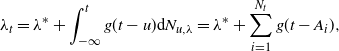 \begin{align*}\lambda_t=\lambda^* + \int_{-\infty}^t g(t-u)\textrm{d}N_{u,\lambda}=\lambda^*+\sum_{i=1}^{N_t} g(t - A_i),\end{align*}
where $g\,:\,\mathbb{R}^+ \to \mathbb{R}^+$
and
$g\,:\,\mathbb{R}^+ \to \mathbb{R}^+$
and $\int_0^\infty g(x) \textrm{d}x < 1$
for stability. One could also consider a marked Hawkes process that draws jump sizes from a sequence of i.i.d. positive random variables
$\int_0^\infty g(x) \textrm{d}x < 1$
for stability. One could also consider a marked Hawkes process that draws jump sizes from a sequence of i.i.d. positive random variables $\{M_i \mid i \in \mathbb{Z}^+\}$
, in which case the summation form of intensity would instead be expressed as
$\{M_i \mid i \in \mathbb{Z}^+\}$
, in which case the summation form of intensity would instead be expressed as
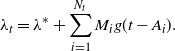 \begin{align*}\lambda_t=\lambda^*+\sum_{i=1}^{N_t} M_i g(t - A_i).\end{align*}
The ESEP model has provided us a natural comparison for the popular Markovian case where $g(x) = \alpha e^{-\beta x}$
(with no marks), but let us now consider more general excitation kernels and jump sizes. To do so, we will make two main generalizations while preserving the other key elements of the ESEP, such as the affine relationship between the intensity and the number of active exciters. First, we will change the activity duration to be a general distribution, mimicking the general excitation kernel. Second, we also change from solitary arrivals to batch arrivals, meaning groups of events that occur simultaneously at each arrival epoch. The sizes of these batches may be drawn from an i.i.d. sequence of positive integer random variables, so we will use the parameter n to represent the relative size of this batch through the mean of the batch size distribution. This leads us to the definition of the nth general ephemerally self-exciting process (n-GESEP).
$g(x) = \alpha e^{-\beta x}$
(with no marks), but let us now consider more general excitation kernels and jump sizes. To do so, we will make two main generalizations while preserving the other key elements of the ESEP, such as the affine relationship between the intensity and the number of active exciters. First, we will change the activity duration to be a general distribution, mimicking the general excitation kernel. Second, we also change from solitary arrivals to batch arrivals, meaning groups of events that occur simultaneously at each arrival epoch. The sizes of these batches may be drawn from an i.i.d. sequence of positive integer random variables, so we will use the parameter n to represent the relative size of this batch through the mean of the batch size distribution. This leads us to the definition of the nth general ephemerally self-exciting process (n-GESEP).
Definition 2. (The nth general ephemerally self-exciting process.) For times $t \geq 0$
, a baseline intensity
$t \geq 0$
, a baseline intensity $\eta^* > 0$
, a cumulative distribution function
$\eta^* > 0$
, a cumulative distribution function $\boldsymbol{G}\,:\,\mathit{\mathbb{R}^+} \rightarrow [0,1]$
, an i.i.d. sequence of positive random variables
$\boldsymbol{G}\,:\,\mathit{\mathbb{R}^+} \rightarrow [0,1]$
, an i.i.d. sequence of positive random variables $\{B_i \mid i \in \mathbb{Z}^+\}$
, and
$\{B_i \mid i \in \mathbb{Z}^+\}$
, and $n \in \mathbb{Z}^+$
such that
$n \in \mathbb{Z}^+$
such that ${\mathbb{E}\!\left[B_i\right]} \in O(n)$
, let
${\mathbb{E}\!\left[B_i\right]} \in O(n)$
, let $N_t(n)$
be a counting process for the arrival epochs occurring according to the stochastic intensity
$N_t(n)$
be a counting process for the arrival epochs occurring according to the stochastic intensity $\eta_t(n)$
, defined to be such that
$\eta_t(n)$
, defined to be such that
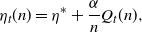 \begin{align}\eta_t(n) = \eta^* + \frac{\alpha}{n} Q_t(n),\end{align}
where $Q_t(n)$
is incremented by
$Q_t(n)$
is incremented by $B_i(n)$
at the ith arrival epoch in
$B_i(n)$
at the ith arrival epoch in $N_t(n)$
and then is depleted at unit down-jumps at the expiration times of the individual arrivals’ activity durations, which are i.i.d. draws from the distribution
$N_t(n)$
and then is depleted at unit down-jumps at the expiration times of the individual arrivals’ activity durations, which are i.i.d. draws from the distribution $G({\cdot})$
across all batches and all epochs. We say that
$G({\cdot})$
across all batches and all epochs. We say that $(\eta_t(n), N_t(n))$
is the nth general ephemerally self-exciting process (n-GESEP).
$(\eta_t(n), N_t(n))$
is the nth general ephemerally self-exciting process (n-GESEP).
It is important to note that in this definition, a batch of size n occurring at the current time would increase the present arrival rate by $\alpha$
. However, these n activity durations are mutually independent. Thus, despite the common arrival epoch, each expiration should cause an instantaneous decrease of just
$\alpha$
. However, these n activity durations are mutually independent. Thus, despite the common arrival epoch, each expiration should cause an instantaneous decrease of just ${\alpha}/{n}$
if the activity duration distribution is continuous. It is also worth noting that this n-GESEP model encapsulates the simple generalization of the ESEP with general service durations, as this is given by
${\alpha}/{n}$
if the activity duration distribution is continuous. It is also worth noting that this n-GESEP model encapsulates the simple generalization of the ESEP with general service durations, as this is given by $(\eta_t(1), N_t(1))$
with
$(\eta_t(1), N_t(1))$
with $\mathbb{P}\left( B_1(1) = 1 \right)$
. Just as the ESEP could be viewed as a Markovian infinite-server queue with a state-dependent arrival rate, the n-GESEP can be seen as an
$\mathbb{P}\left( B_1(1) = 1 \right)$
. Just as the ESEP could be viewed as a Markovian infinite-server queue with a state-dependent arrival rate, the n-GESEP can be seen as an $\textrm{M}^B$
/G/
$\textrm{M}^B$
/G/ $\infty$
queue with a state-dependent arrival rate. This perspective implies the existence and uniqueness of Definition 2.
$\infty$
queue with a state-dependent arrival rate. This perspective implies the existence and uniqueness of Definition 2.
Just as it is often beneficial to think of the length of an infinite-server queue as a sum over all customers that remain in service, it will be quite useful for us to think about the number active within the n-GESEP as the sum of all arrivals that have not yet expired. For $A_i$
as the ith arrival epoch and
$A_i$
as the ith arrival epoch and $S_{i,j}$
as the jth activity duration within the ith batch, this can be expressed as
$S_{i,j}$
as the jth activity duration within the ith batch, this can be expressed as
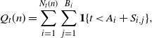 \begin{align*}Q_t(n) = \sum_{i=1}^{N_t(n)} \sum_{j=1}^{B_i} \textbf{1}\{t < A_i + S_{i,j}\},\end{align*}
or equivalently for the intensity,
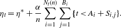 \begin{align*}\eta_t = \eta^* + \frac{\alpha}{n} \sum_{i=1}^{N_t(n)} \sum_{j=1}^{B_i} \textbf\{t < A_i + S_{i,j}\}.\end{align*}
A nice consequence of this representation is that the ephemerality is at the forefront. Because the event within the indicator is that the current time t is less than the sum of a given arrival time and activity duration, this indicator counts whether that particular excitement is currently active. Thus, this indicator will switch from 1 to 0 when the present time passes a given expiration time, causing the intensity to drop by $\alpha / n$
. From this point forward, the excitement brought by this particular arrival no longer has a direct effect on the system.
$\alpha / n$
. From this point forward, the excitement brought by this particular arrival no longer has a direct effect on the system.
We will now use the n-GESEP to establish a main result of this work, in which we connect this general form of ephemeral self-excitement to general forms of the traditional, eternal notion of self-excitement. In Theorem 2, we prove a scaling limit that incorporates random batch distributions and general service to construct marked, general decay Hawkes processes. We refer to this limit as a ‘batch scaling’, as we are letting the relative batch size n grow large, which simultaneously shrinks the size of the excitement generated by each individual entity within a batch of arrivals. Thus, while the effect of one individual exciter shrinks, the collective effect of a batch arrival remains fixed. In the limit, this provides an alternate construction of the Hawkes process.
Theorem 2. For $t \geq 0$
and
$t \geq 0$
and $n \in \mathbb{Z}^+$
, let
$n \in \mathbb{Z}^+$
, let $(\eta_t(n), N_t(n))$
be an n-GESEP with baseline intensity
$(\eta_t(n), N_t(n))$
be an n-GESEP with baseline intensity $\eta^* > 0$
, intensity jump size
$\eta^* > 0$
, intensity jump size $\alpha > 0$
, activity duration cumulative distribution function
$\alpha > 0$
, activity duration cumulative distribution function $G({\cdot})$
, and i.i.d. batch size sequence of nonnegative, discrete random variables
$G({\cdot})$
, and i.i.d. batch size sequence of nonnegative, discrete random variables $\{B_i \mid i \in \mathbb{Z}^+\}$
. Additionally, let
$\{B_i \mid i \in \mathbb{Z}^+\}$
. Additionally, let $\eta_0(n) = \eta^*$
, i.e.
$\eta_0(n) = \eta^*$
, i.e. $Q_0(n) = 0$
. Then, for all
$Q_0(n) = 0$
. Then, for all $t \geq 0$
, this n-GESEP process is such that
$t \geq 0$
, this n-GESEP process is such that
 \begin{align} \eta_t(n)\stackrel{D}{\Longrightarrow}\lambda_t\text{ and }N_t(n)\stackrel{D}{\Longrightarrow}N_{t,\lambda}\end{align}
as $n \to \infty$
, where
$n \to \infty$
, where $(\lambda_t, N_{t,\lambda})$
is the general Hawkes process intensity and counting process pair such that
$(\lambda_t, N_{t,\lambda})$
is the general Hawkes process intensity and counting process pair such that
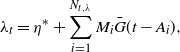 \begin{align}\lambda_t=\eta^*+\sum_{i=1}^{N_{t,\lambda}}M_i\bar G(t-A_i),\end{align}
where $\{A_i \mid i \in \mathbb{Z}^+\}$
are the Hawkes process arrival epochs,
$\{A_i \mid i \in \mathbb{Z}^+\}$
are the Hawkes process arrival epochs, $\bar G(x) = 1 - G(x)$
for all
$\bar G(x) = 1 - G(x)$
for all $x \geq 0$
, and
$x \geq 0$
, and $\{M_i \mid i \in \mathbb{Z}^+\}$
is an i.i.d. sequence of positive real random variables such that
$\{M_i \mid i \in \mathbb{Z}^+\}$
is an i.i.d. sequence of positive real random variables such that ${\alpha B_1}/{n} \stackrel{D}{\Longrightarrow} M_1$
and
${\alpha B_1}/{n} \stackrel{D}{\Longrightarrow} M_1$
and ${B_1}/{n^2} \stackrel{p}{\longrightarrow} 0$
.
${B_1}/{n^2} \stackrel{p}{\longrightarrow} 0$
.
Proof. We will organize the proof into two parts. Each part is oriented around the process arrival times, as these fully determine the sample path of the Hawkes process. We will first show through induction that the distributions of inter-arrival times converge. Then we will demonstrate that given the same arrival times, the dynamics of the processes converge.
To begin, let $A_i^\eta$
for
$A_i^\eta$
for $i \in \mathbb{Z}^+$
be the time of the ith arrival in the n-GESEP, and similarly let
$i \in \mathbb{Z}^+$
be the time of the ith arrival in the n-GESEP, and similarly let $A^\lambda_i$
be the ith arrival time for the Hawkes process. We start with the base case: for the time of the first arrival, we can note that for all n-GESEP models,
$A^\lambda_i$
be the ith arrival time for the Hawkes process. We start with the base case: for the time of the first arrival, we can note that for all n-GESEP models,
 \begin{align*}\mathbb{P}\left( A_1^\eta > x \right) = e^{-\eta^* x},\end{align*}
as $Q_0(n) = 0$
and thus the first arrival is driven by the external baseline rate. Likewise, for the Hawkes process, since (17) implies that
$Q_0(n) = 0$
and thus the first arrival is driven by the external baseline rate. Likewise, for the Hawkes process, since (17) implies that $\lambda_t = \nu^*$
for
$\lambda_t = \nu^*$
for $0 \leq t < A_1^\lambda$
, we can see that
$0 \leq t < A_1^\lambda$
, we can see that
 \begin{align*}\mathbb{P}\left( A_1^\lambda > x \right) = e^{-\eta^* x},\end{align*}
and thus $\mathbb{P}\left( A_1^\lambda > x \right) = \mathbb{P}\left( A_1^\eta > x \right)$
. As an inductive hypothesis, we now assume that
$\mathbb{P}\left( A_1^\lambda > x \right) = \mathbb{P}\left( A_1^\eta > x \right)$
. As an inductive hypothesis, we now assume that $\{A_1^\eta, \dots, A_k^\eta\}$
converge in joint and marginal distributions to
$\{A_1^\eta, \dots, A_k^\eta\}$
converge in joint and marginal distributions to $\{A_1^\lambda, \dots, A_k^\lambda\}$
where
$\{A_1^\lambda, \dots, A_k^\lambda\}$
where $k \in \mathbb{Z}^+$
. Now, for the Hawkes process we can observe that
$k \in \mathbb{Z}^+$
. Now, for the Hawkes process we can observe that
 \begin{align*}\textrm{P}_k\left(A_{k+1}^\lambda - A_{k}^\lambda > x\right)&\,:\!=\,\mathbb{P}\left( A_{k+1}^\lambda - A_{k}^\lambda > x \mid \{A_1^\lambda, \dots, A_k^\lambda\} \right)=\textrm{E}_k\left[ e^{-\int_{0}^{x} \lambda_{A_k^\lambda + t} \textrm{d}t} \right],\end{align*}
because when conditioned on the arrival history, the Hawkes process behaves like an inhomogeneous Poisson process until the next arrival occurs. Using (17), we can express this as
 \begin{align*}\textrm{E}_k\left[ e^{-\int_{0}^{x} \lambda_{A_k^\lambda + t} \textrm{d}t} \right]&=e^{-\eta^* x} \textrm{E}_k\left[ e^{-\int_{0}^{x} \sum_{i=1}^k M_i \bar G \left(A_k^\lambda - A_i^\lambda + t\right) \textrm{d}t} \right]\\&=e^{-\eta^* x} \prod_{i=1}^k \textrm{E}_k\left[ e^{- M_i \int_{0}^{x} \bar G \left(A_k^\lambda - A_i^\lambda + t\right) \textrm{d}t} \right]\!.\end{align*}
Turning to the ESEP epochs, we define $N_{i,j}^\eta\left( (t, t+s]\right)$
as the number of arrivals on the time interval
$N_{i,j}^\eta\left( (t, t+s]\right)$
as the number of arrivals on the time interval $(t, t+s]$
that are generated by the excitement caused by the jth entity within the ith batch. Furthermore, let
$(t, t+s]$
that are generated by the excitement caused by the jth entity within the ith batch. Furthermore, let $N_{*}^\eta\left( (t, t+s]\right)$
be the number of arrivals on
$N_{*}^\eta\left( (t, t+s]\right)$
be the number of arrivals on $(t, t+s]$
that are generated by the external, baseline rate
$(t, t+s]$
that are generated by the external, baseline rate $\eta^*$
. Then, using this notation, we have that
$\eta^*$
. Then, using this notation, we have that
 \begin{align*}\textrm{P}_k\left(A_{k+1}^\eta - A_{k}^\eta > x\right)&\,:\!=\,\mathbb{P}\left( A_{k+1}^\eta - A_{k}^\eta > x \mid \{A_1^\eta, \dots, A_k^\eta\} \right)\\&=\textrm{P}_k\left( \bigcap_{i=1}^k \bigcap_{j=1}^{B_i} \left\{N_{i,j}^\eta\left( (A_k^\eta, A_{k}^\eta+x]\right) = 0\right\} \cap \left\{N_{*}^\eta\left( (A_k^\eta, A_{k}^\eta+x]\right) = 0\right\} \right)\\&=\textrm{E}_k\left[ \prod_{i=1}^k \prod_{j=1}^{B_i} \textbf{1}\left\{N_{i,j}^\eta\left( (A_k^\eta, A_{k}^\eta+x]\right) = 0\right\} \textbf{1}\left\{N_{*}^\eta\left( (A_k^\eta, A_{k}^\eta+x]\right) = 0\right\} \right]\!.\end{align*}
From the independence of each of these arrival processes, we can move the probability for no arrivals in the external arrival process and the product over i outside of the expectation to obtain
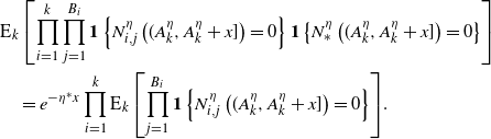 \begin{align*}&\textrm{E}_k\left[ \prod_{i=1}^k \prod_{j=1}^{B_i} \textbf{1}\left\{N_{i,j}^\eta\left( (A_k^\eta, A_{k}^\eta+x]\right) = 0\right\} \textbf{1}\left\{N_{*}^\eta\left( (A_k^\eta, A_{k}^\eta+x]\right) = 0\right\} \right]\\&\quad=e^{-\eta^* x}\prod_{i=1}^k \textrm{E}_k\left[ \prod_{j=1}^{B_i} \textbf{1}\left\{N_{i,j}^\eta\left( (A_k^\eta, A_{k}^\eta+x]\right) = 0\right\} \right]\!.\end{align*}
Consider an arbitrary entity, say the jth entity in the ith batch. Let $S_{i,j}$
be its service duration. If this entity has departed from the queue before
$S_{i,j}$
be its service duration. If this entity has departed from the queue before $A_k^\eta$
, then it cannot generate further arrivals, and thus
$A_k^\eta$
, then it cannot generate further arrivals, and thus
 \begin{align*}\textrm{P}_k\left( N_{i,j}^\eta\left( (A_k^\eta, A_{k}^\eta+x]\right) = 0 \mid S_{i,j} \leq A_k^\eta - A_i^\eta\right) = 1.\end{align*}
Likewise, if it does not depart until after $A_k^\eta + x$
, then the probability that it generates an arrival on
$A_k^\eta + x$
, then the probability that it generates an arrival on $(A_k^\eta, A_{k}^\eta+x]$
is
$(A_k^\eta, A_{k}^\eta+x]$
is
 \begin{align*}\textrm{P}_k\left( N_{i,j}^\eta\left( (A_k^\eta, A_{k}^\eta+x]\right) = 0 \mid S_{i,j} \geq A_k^\eta - A_i^\eta + x\right) = e^{-\frac{\alpha}{n}x}.\end{align*}
Finally, if the entity departs in the interval $(A_k^\eta, A_{k}^\eta+x]$
, the probability that it generates an arrival before departing is
$(A_k^\eta, A_{k}^\eta+x]$
, the probability that it generates an arrival before departing is
 \begin{align*}\textrm{P}_k\left( N_{i,j}^\eta\left( (A_k^\eta, A_{k}^\eta+x]\right) = 0 \mid S_{i,j} = A_k^\eta - A_i^\eta + z\right) = e^{-\frac{\alpha}{n}z},\end{align*}
where $0 < z < x$
. Therefore, through conditioning on each entity’s service duration, we have that
$0 < z < x$
. Therefore, through conditioning on each entity’s service duration, we have that
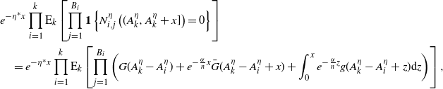 \begin{align*}&e^{-\eta^* x}\prod_{i=1}^k \textrm{E}_k\left[ \prod_{j=1}^{B_i} \textbf{1}\left\{N_{i,j}^\eta\left( (A_k^\eta, A_{k}^\eta+x]\right) = 0\right\} \right]\\&\quad=e^{-\eta^* x}\prod_{i=1}^k \textrm{E}_k\left[ \prod_{j=1}^{B_i} \left( G(A^\eta_k - A^\eta_i) + e^{-\frac{\alpha}{n}x}\bar{G}(A^\eta_k - A^\eta_i + x) + \int_0^x e^{-\frac{\alpha}{n}z}g(A_k^\eta - A_i^\eta +z)\textrm{d}z\right) \right],\end{align*}
where $g({\cdot})$
is the density corresponding to
$g({\cdot})$
is the density corresponding to $G({\cdot})$
. Since the term inside the inner product does not depend on the specific entity within a batch but only on the batch itself, we can evaluate this inside the expectation as
$G({\cdot})$
. Since the term inside the inner product does not depend on the specific entity within a batch but only on the batch itself, we can evaluate this inside the expectation as
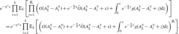 \begin{align*}&e^{-\eta^* x}\prod_{i=1}^k \textrm{E}_k\left[ \prod_{j=1}^{B_i} \left( G(A^\eta_k - A^\eta_i) + e^{-\frac{\alpha}{n}x}\bar{G}(A^\eta_k - A^\eta_i + x) + \int_0^x e^{-\frac{\alpha}{n}z}g(A_k^\eta - A_i^\eta +z)\textrm{d}z\right) \right]\\&\quad=e^{-\eta^* x}\prod_{i=1}^k \textrm{E}_k\left[ \left( G(A^\eta_k - A^\eta_i) + e^{-\frac{\alpha}{n}x}\bar{G}(A^\eta_k - A^\eta_i + x) + \int_0^x e^{-\frac{\alpha}{n}z}g(A_k^\eta - A_i^\eta +z)\textrm{d}z\right)^{B_i} \right]\!.\end{align*}
Since the base term of this exponent is deterministic, we will simplify it as follows. Using integration by parts on $\int_0^x e^{-\frac{\alpha}{n}z}g(A_k^\eta - A_i^\eta +z)\textrm{d}z$
and expanding
$\int_0^x e^{-\frac{\alpha}{n}z}g(A_k^\eta - A_i^\eta +z)\textrm{d}z$
and expanding $\bar{G}(x) = 1 - G(x)$
, we obtain
$\bar{G}(x) = 1 - G(x)$
, we obtain
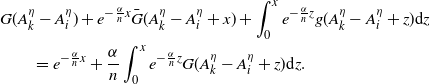 \begin{align*}&G(A^\eta_k - A^\eta_i) + e^{-\frac{\alpha}{n}x}\bar{G}(A^\eta_k - A^\eta_i + x) + \int_0^x e^{-\frac{\alpha}{n}z}g(A_k^\eta - A_i^\eta +z)\textrm{d}z\\&\qquad =e^{-\frac{\alpha}{n}x} + \frac{\alpha}{n}\int_0^x e^{-\frac{\alpha}{n}z}G(A_k^\eta - A_i^\eta +z)\textrm{d}z.\end{align*}
If we express $e^{-\frac{\alpha}{n}x}$
in integral form via
$e^{-\frac{\alpha}{n}x}$
in integral form via $e^{-\frac{\alpha}{n}x} = 1 - \frac{\alpha}{n}\int_0^x e^{-\frac{\alpha}{n}z}\textrm{d}z$
, we can further simplify this expression for the base to
$e^{-\frac{\alpha}{n}x} = 1 - \frac{\alpha}{n}\int_0^x e^{-\frac{\alpha}{n}z}\textrm{d}z$
, we can further simplify this expression for the base to
 \begin{align*}e^{-\frac{\alpha}{n}x} + \frac{\alpha}{n}\int_0^x e^{-\frac{\alpha}{n}z}G(A_k^\eta - A_i^\eta +z)\textrm{d}z&=1 - \frac{\alpha}{n}\int_0^x e^{-\frac{\alpha}{n}z} \bar{G}(A_k^\eta - A_i^\eta + z) \textrm{d}z.\end{align*}
This form makes it quick to observe that this base term is at most 1. Thus we are justified in taking the expectation of this term raised to $B_i$
, since that is equivalent to the probability generating function of the batch size, and this exists for all discrete random variables when evaluated on values less than or equal to 1 in absolute value. Returning to this expectation, we first note that for all x, rearranging the Taylor expansion of
$B_i$
, since that is equivalent to the probability generating function of the batch size, and this exists for all discrete random variables when evaluated on values less than or equal to 1 in absolute value. Returning to this expectation, we first note that for all x, rearranging the Taylor expansion of $e^x$
produces
$e^x$
produces
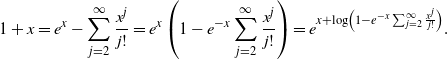 \begin{align*}1 + x&=e^{x} - \sum_{j=2}^\infty \frac{x^j}{j!}=e^x\left(1 - e^{-x} \sum_{j=2}^\infty \frac{x^j}{j!}\right)=e^{x + \log\left(1 - e^{-x} \sum_{j=2}^\infty \frac{x^j}{j!}\right)}.\end{align*}
Thus we re-express the expectation in exponential function form as
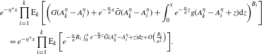 \begin{align*}&e^{-\eta^* x}\prod_{i=1}^k \textrm{E}_k\left[ \left( G(A^\eta_k - A^\eta_i) + e^{-\frac{\alpha}{n}x}\bar{G}(A^\eta_k - A^\eta_i) + \int_0^x e^{-\frac{\alpha}{n}z}g(A_k^\eta - A_i^\eta +z)\textrm{d}z\right)^{B_i} \right]\\&\quad=e^{-\eta^* x}\prod_{i=1}^k \textrm{E}_k\left[ e^{- \frac{\alpha}{n}B_i\int_0^x e^{-\frac{\alpha}{n}z} \bar{G}(A_k^\eta - A_i^\eta + z) \textrm{d}z + O\left(\frac{B_i}{n^2} \right)} \right]\!.\end{align*}
Through use of a Taylor expansion on $e^{-\frac{\alpha}{n}z}$
and absorbing higher terms into the
$e^{-\frac{\alpha}{n}z}$
and absorbing higher terms into the $O\left(\frac{B_i}{n^2} \right)$
notation, we can further simplify to
$O\left(\frac{B_i}{n^2} \right)$
notation, we can further simplify to
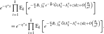 \begin{align*}&e^{-\eta^* x}\prod_{i=1}^k \textrm{E}_k\left[ e^{- \frac{\alpha}{n}B_i\int_0^x e^{-\frac{\alpha}{n}z} \bar{G}(A_k^\eta - A_i^\eta + z) \textrm{d}z + O\left(\frac{B_i}{n^2} \right)} \right]\\&\qquad =e^{-\eta^* x}\prod_{i=1}^k \textrm{E}_k\left[ e^{- \frac{\alpha}{n}B_i\int_0^x \bar{G}(A_k^\eta - A_i^\eta + z) \textrm{d}z + O\left(\frac{B_i}{n^2} \right)} \right]\!.\end{align*}
We can now take the limit as $n \to \infty$
and observe that
$n \to \infty$
and observe that
 \begin{align*}e^{-\eta^* x}\prod_{i=1}^k \textrm{E}_k\left[ e^{- \frac{\alpha}{n}B_i\int_0^x \bar{G}(A_k^\eta - A_i^\eta + z) \textrm{d}z + O\left(\frac{B_i}{n^2} \right)} \right]&\longrightarrow e^{-\eta^* x}\prod_{i=1}^k \textrm{E}_k\left[ e^{- M_i \int_0^x \bar{G}(A_k^\eta - A_i^\eta + z) \textrm{d}z } \right],\end{align*}
as we have that $\frac{\alpha}{n}B_1 \stackrel{D}{\Longrightarrow} M_1$
and
$\frac{\alpha}{n}B_1 \stackrel{D}{\Longrightarrow} M_1$
and $\frac{B_i}{n^2} \stackrel{D}{\Longrightarrow} 0$
. This is equal to the Hawkes process inter-arrival probability
$\frac{B_i}{n^2} \stackrel{D}{\Longrightarrow} 0$
. This is equal to the Hawkes process inter-arrival probability $\textrm{P}_k\left(A_{k+1}^\lambda - A_{k}^\lambda > x\right)$
. Hence by induction and total probability the arrival times converge, completing the first part of the proof.
$\textrm{P}_k\left(A_{k+1}^\lambda - A_{k}^\lambda > x\right)$
. Hence by induction and total probability the arrival times converge, completing the first part of the proof.
For the second part of the proof, we show that the dynamics of the processes converge when we condition on having the same fixed arrival times, which we now denote by $\{A_i \mid i \in \mathbb{Z}^+\}$
for both processes. Since
$\{A_i \mid i \in \mathbb{Z}^+\}$
for both processes. Since $N_t(n)$
is defined as the counting process of arrival epochs rather than total number of arrivals,
$N_t(n)$
is defined as the counting process of arrival epochs rather than total number of arrivals, $N_t(n) = N_{t,\lambda}$
for all n and all t. We now treat the intensity in two cases, the jump at arrivals and the dynamics between these times. For the first case, we take
$N_t(n) = N_{t,\lambda}$
for all n and all t. We now treat the intensity in two cases, the jump at arrivals and the dynamics between these times. For the first case, we take $k \in \mathbb{Z}^+$
and let
$k \in \mathbb{Z}^+$
and let $\lambda_{A_{k^-}} = \inf_{A_{k-1} \leq t < A_k} \lambda_t$
and
$\lambda_{A_{k^-}} = \inf_{A_{k-1} \leq t < A_k} \lambda_t$
and $\eta_{A_{k^-}}(n) = \inf_{A_{k-1} \leq t < A_k} \eta_t(n)$
for all n, where
$\eta_{A_{k^-}}(n) = \inf_{A_{k-1} \leq t < A_k} \eta_t(n)$
for all n, where $A_0 = 0$
. Then the jump in the n-GESEP intensity at the kth jump is such that
$A_0 = 0$
. Then the jump in the n-GESEP intensity at the kth jump is such that
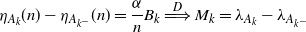 \begin{align*}\eta_{A_k}(n) - \eta_{A_{k^-}}(n)&=\frac{\alpha}{n}B_k\stackrel{D}{\Longrightarrow} M_k=\lambda_{A_k} - \lambda_{A_{k^-}}\end{align*}
as $n \to \infty$
. For the behavior between arrival times we first note that for
$n \to \infty$
. For the behavior between arrival times we first note that for $S_j$
independent and distributed with cumulative distribution function
$S_j$
independent and distributed with cumulative distribution function $G({\cdot})$
for all
$G({\cdot})$
for all $j \in \mathbb{Z}^+$
, the probability generating function of
$j \in \mathbb{Z}^+$
, the probability generating function of $\frac{1}{n}\sum_{j=1}^{B_1}\textbf{1}\{y < S_j\}$
is
$\frac{1}{n}\sum_{j=1}^{B_1}\textbf{1}\{y < S_j\}$
is
 \begin{align*}{\mathbb{E}\!\left[z^{\frac{1}{n}\sum_{j=1}^{B_1}\textbf{1}\{y < S_j\}}\right]}&={\mathbb{E}\!\left[\left(G(y) + \bar{G}(y) z^{\frac{1}{n}} \right)^{B_1}\right]}={\mathbb{E}\!\left[\left(1 - \bar{G}(y) \left(1 - e^{\frac{1}{n}\log{z}}\right) \right)^{B_1}\right]},\end{align*}
and by a Taylor expansion approach similar to what we used in the first part of the proof, we can see that
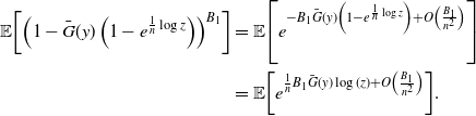 \begin{align*}{\mathbb{E}\!\left[\left(1 - \bar{G}(y) \left(1 - e^{\frac{1}{n}\log{z}}\right) \right)^{B_1}\right]}&={\mathbb{E}\!\left[e^{- B_1\bar{G}(y) \left(1 - e^{\frac{1}{n}\log{z}}\right) + O\left(\frac{B_1}{n^2}\right)}\right]}\\&={\mathbb{E}\!\left[e^{\frac{1}{n}B_1\bar{G}(y) \log(z) + O\left(\frac{B_1}{n^2}\right)}\right]}.\end{align*}
Taking the limit as $n \to \infty$
, this yields
$n \to \infty$
, this yields
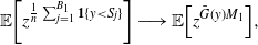 \begin{align*}{\mathbb{E}\!\left[z^{\frac{1}{n}\sum_{j=1}^{B_1}\textbf{1}\{y < S_j\}}\right]}\longrightarrow {\mathbb{E}\!\left[z^{\bar{G}(y)M_1}\right]},\end{align*}
which is to say that
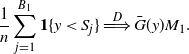 \begin{align*}\frac{1}{n}\sum_{j=1}^{B_1}\textbf{1}\{y < S_j\} \stackrel{D}{\Longrightarrow} \bar{G}(y)M_1.\end{align*}
Using this, we can now see that for $k \in \mathbb{Z}^+$
and
$k \in \mathbb{Z}^+$
and $0 \leq x < A_{k+1} - A_{k}$
, the intensity of the n-GESEP satisfies
$0 \leq x < A_{k+1} - A_{k}$
, the intensity of the n-GESEP satisfies
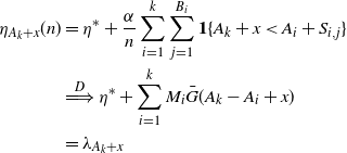 \begin{align*}\eta_{A_k + x}(n)&=\eta^* + \frac{\alpha}{n} \sum_{i=1}^k \sum_{j=1}^{B_i} \textbf{1}\{A_k + x < A_i + S_{i,j} \}\\&\stackrel{D}{\Longrightarrow}\eta^*+\sum_{i=1}^k M_i \bar{G}(A_k - A_i + x)\\&=\lambda_{A_k + x}\end{align*}
as $n \to \infty$
. Thus, both the jump sizes of
$n \to \infty$
. Thus, both the jump sizes of $\eta_t(n)$
and the behavior of
$\eta_t(n)$
and the behavior of $\eta_t(n)$
between jumps converge to those of
$\eta_t(n)$
between jumps converge to those of $\lambda_t$
, completing the proof.
$\lambda_t$
, completing the proof.
For an empirical demonstration of this convergence, in Figure 5 we plot cumulative distribution functions for the intensities and counts of the n-GESEP across increasing batch sizes and multiple expiration distributions and compare them to the empirical distributions of the corresponding general Hawkes processes. Specifically, we consider three different choices of $\bar{G}({\cdot})$
, all with a unit mean expiration time: a standard exponential
$\bar{G}({\cdot})$
, all with a unit mean expiration time: a standard exponential $\bar G(x) = e^{-x}$
, a two-phase Erlang distribution
$\bar G(x) = e^{-x}$
, a two-phase Erlang distribution $\bar G(x) = (1+2x)e^{-2x}$
, and a two-phase hyper-exponential
$\bar G(x) = (1+2x)e^{-2x}$
, and a two-phase hyper-exponential $\bar G(x) = (e^{-2x} + e^{-2/3 x})/2$
. Each experiment is conducted for deterministic batch sizes in the n-GESEP models and deterministic marks in the Hawkes processes. Similar performance was observed for other distributions such as the geometric (or exponential in limiting form) and are thus omitted for brevity. In each of the three distribution settings with batch size
$\bar G(x) = (e^{-2x} + e^{-2/3 x})/2$
. Each experiment is conducted for deterministic batch sizes in the n-GESEP models and deterministic marks in the Hawkes processes. Similar performance was observed for other distributions such as the geometric (or exponential in limiting form) and are thus omitted for brevity. In each of the three distribution settings with batch size $n = 8$
in the n-GESEP model, the distribution of the intensity is quite close to that of the Hawkes intensity, as can be seen in the left-hand column. On the right, one can note that the count distributions are quite close in all the various settings, and again the performance is particularly strong by
$n = 8$
in the n-GESEP model, the distribution of the intensity is quite close to that of the Hawkes intensity, as can be seen in the left-hand column. On the right, one can note that the count distributions are quite close in all the various settings, and again the performance is particularly strong by $n = 8$
. The visible closeness of these count distributions—indeed, they are nearly indistinguishable—lends added importance to the calculations in Proposition 4. Given these observations, it is of particular interest to study the convergence rates of these models in future work.
$n = 8$
. The visible closeness of these count distributions—indeed, they are nearly indistinguishable—lends added importance to the calculations in Proposition 4. Given these observations, it is of particular interest to study the convergence rates of these models in future work.
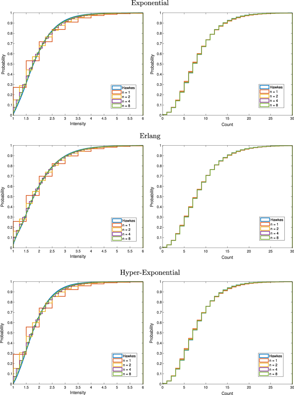
Figure 5. Empirical transient distributions of the intensities (left) and counts (right) of n-GESEP with increasing batch size and for general Hawkes process simulations with $t = 5$
,
$t = 5$
, $\eta^* = 1$
,
$\eta^* = 1$
, $\alpha = 0.5$
, and varying expiration distributions. These distributions are calculated from
$\alpha = 0.5$
, and varying expiration distributions. These distributions are calculated from $2^{22}$
replications.
$2^{22}$
replications.
As a reference, we list the components of the ephemerally self-exciting models and their corresponding limiting quantities in the general Hawkes process below in Table 1. We can note that because the limiting excitation kernel given in Theorem 2 is a complementary cumulative distribution function it is exclusively non-increasing, meaning that the excitement after each arrival immediately decays. It can be observed that this includes the two most popular excitation kernels, the exponential and power-law forms that we detailed in Subsection 2.1. However, it does not include kernels that have the ‘hump remote from the origin’ that Hawkes mentions briefly in the original paper [Reference Hawkes36]. If desired, this can be remedied through extension to multi-phase service in the n-GESEP, with the intensity defined as an affine relationship with one of the later phases.
Table 1. Overview of convergence details in the batch scaling of the ESEP.
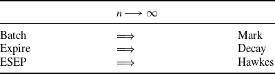
Before concluding, let us remark that in addition to providing conceptual understanding into the Hawkes process itself, the alternate construction through the batch scaling in Theorem 2 is also of practical relevance in explaining the use of the Hawkes process in many applications. For example, in biological applications such as the environmental management problem considered in [Reference Gupta, Farajtabar, Dilkina and Zha32], one of the invasive species studied may produce multiple offspring simultaneously but only for the duration of its life cycle. That is, many species give birth in litters, creating batch arrivals, but of course reproduce only during their lifetimes, yielding ephemerality. Furthermore, the numerical experiments in Figure 5 suggest that n need not be overly large for the n-GESEP and the Hawkes process to be comparable in distribution.
As another example, consider the spread of information on communication and social media platforms. This setting has recently been a popular application of Hawkes processes; see e.g. [Reference Du22, Reference Farajtabar26, Reference Halpin and De Boeck34, Reference Rizoiu54, Reference Rizoiu55]. When a user shares a post on these platforms, it is immediately and simultaneously dispatched to the real-time feeds of many other users, creating a batch increase of the response rate from the other users. The post then will typically only be seen on news feeds for a short period of time, as new content comes in to replace it. On top of this, social media administrators have been adopting a trend of intentionally introducing ephemerality into their platforms. For example, the expiration of posts and messages has been a defining feature of Snapchat since its inception. Facebook and Instagram have recently adopted the same behavior with ‘stories’, and Twitter has responded in kind with the appropriately named ‘fleets’. Just as in the case of biological offspring processes, Theorem 2 offers an explanation of why the Hawkes process has become a popular and successful model in this space. Moreover, the insights from these connections can be deepened through the additional model relationships that we have discussed in Section 3.
5. Conclusion
Time is fleeting; excitement is ephemeral. In this paper we have introduced the ephemerally self-exciting process (ESEP), a point process driven by the pieces of its history that remain presently active. That is, each arrival excites the arrival rate until the expiration of its randomly drawn activity duration, at which point its individual influence vanishes. Throughout this work we have compared ephemeral self-excitement to eternal self-excitement through contrast with the well-known Hawkes process. These comparisons include an ordering of the moments of the two processes in Proposition 2 and a study of each process’s branching structure in Subsection 3.1. We have also used the ESEP to relate ephemeral self-excitement to other well-known stochastic models, including preferential attachment, random walks, and epidemics. Finally, we have also considered a generalized model with batch arrivals and general activity duration distributions, which we refer to as the nth general ephemerally self-exciting process (n-GESEP). The n-GESEP model provides an alternate construction of general marked Hawkes processes through a batch scaling limit. ln Theorem 2 we prove that the n-GESEP model converges to a Hawkes process as its batch arrival size grows large, with the limiting Hawkes process having an excitation kernel matching the tail cumulative distribution function of the activity duration distribution, and having marks given by the scaled limit of the batch sizes. As we have discussed, this limit both provides intuition for the occurrence of self-excitement in natural phenomena and relates the Hawkes process to the other stochastic models we connected to ephemeral self-excitement.
This presents many directions for future research. First, we have frequently emphasized in this work that our results motivate the ESEP (and by extension the n-GESEP) as a promising model for self-excitement in its own right. This follows from its tractability for analysis and its amenability to connection with other models. Because of this promise, we believe that further exploration and application of the ESEP holds great potential. Another natural and relevant avenue would be to continue to explore the connection between ephemeral self-excitement and the other stochastic models we have discussed. For example, one could study the connection between ESEP and epidemic models on more complex networks or with more complex dynamics. Doing so would give a point process representation for the times of infection in a more realistic epidemic model, which could be quite useful in practice for resource allocation and policy design. Similar deepened connections could also be pursued for other models, such as preferential attachment. In general, we believe the concept of ephemeral self-excitement merits further theoretical exploration and detailed empirical application, both of which we look forward to pursuing. Finally, to empower this model for full practical use, it is of great interest to study the estimation of the ESEP and n-GESEP processes. For example, likelihood-based estimation could be pursued in a manner similar to that used for the traditional Hawkes process, since the processes are also conditionally non-stationary Poisson when given the full history. In fact, similar estimation techniques may be achievable even if the data contains only arrival epochs (and not expiration times), perhaps through missing data techniques such as expectation–maximization algorithms. These methods have been applied successfully both for Hawkes processes and generally for branching processes (see, e.g., [Reference Lewis and Mohler43, Reference Veen and Schoenberg59]), and thus also hold potential for the ephemerally self-exciting models we have studied here.
Appendix A. Lemmas and auxiliaries
In this section of the appendix we give technical lemmas to support our analysis and brief auxiliary results that are of interest but not within the narrative of the body of this report. We begin by giving the infinitesimal generator form for time derivatives of the expectations of functions of our process. This is a valuable tool available to us because the ESEP is Markov, and it supports much of our analysis throughout this work.
Lemma 2. For a sufficiently regular function $f\,:\,\left(\mathbb{R}^+ \times \mathbb{N}\right) \to \mathbb{R}$
, the generator of the ESEP is given by
$f\,:\,\left(\mathbb{R}^+ \times \mathbb{N}\right) \to \mathbb{R}$
, the generator of the ESEP is given by
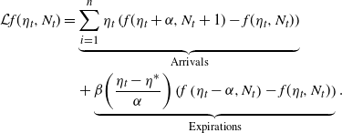 \begin{align}\mathcal{L}f(\eta_t, N_t)&=\underbrace{\sum_{i=1}^n \eta_t \left( f(\eta_t + \alpha, N_t + 1) - f(\eta_t, N_t) \right)}_{\textrm{Arrivals}}\nonumber \\&\quad +\underbrace{ \beta\! \left(\frac{\eta_t - \eta^*}{\alpha} \right)\left(f\left(\eta_t - \alpha, N_t\right) - f(\eta_t, N_t)\right)}_{\textrm{Expirations}}.\end{align}
Then, the time derivative of the expectation of $f(\eta_t, N_t)$
is given by
$f(\eta_t, N_t)$
is given by
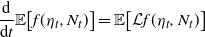 \begin{equation}\frac{\textrm{d}}{\textrm{d}t} {\mathbb{E}\!\left[f(\eta_t, N_t)\right]}={\mathbb{E}\!\left[\mathcal{L}f(\eta_t, N_t)\right]}\end{equation}
for all $t \geq 0$
.
$t \geq 0$
.
Proof. This is a direct result of the ESEP belonging to the family of piecewise deterministic Markov processes, as defined in [Reference Davis19]. Moreover, the specific regularity conditions are given in Theorem 5.5 of that work.
Note that this is also immediately applicable to the active-number-in-system process perspective on the ESEP, as $Q_t = (\eta_t - \eta^*)/\alpha$
. Thus, we leverage this infinitesimal generator to study each of
$Q_t = (\eta_t - \eta^*)/\alpha$
. Thus, we leverage this infinitesimal generator to study each of $\eta_t$
,
$\eta_t$
, $Q_t$
, and
$Q_t$
, and $N_t$
throughout both the main body of the text and these appendices.
$N_t$
throughout both the main body of the text and these appendices.
As another supporting lemma, let us summarize a result that can be used with the infinitesimal generator to relate two different Markov processes. Throughout this work we make comparisons between different processes, in particular between the ESEP and the Hawkes process. One way that we do this is by investigating the differential equations found with the use of Lemma 2. In Lemma 3 we provide the method by which we make such comparisons.
Lemma 3. (A comparison lemma.) Let $f\,:\, \mathbb{R}^2 \to \mathbb{R}$
be a continuous function in both variables. If we assume that the initial value problem
$f\,:\, \mathbb{R}^2 \to \mathbb{R}$
be a continuous function in both variables. If we assume that the initial value problem
 \begin{equation}\frac{\textrm{d}x(t)}{\textrm{d}t} = f(t, x(t)), \ x(0) = x_0\end{equation}
has a unique solution for the time interval [0, T], and
 \begin{equation}\frac{\textrm{d}y(t)}{\textrm{d}t} \leq f(t, y(t)) \quad \textrm{for} \ t \in [0,T] \ \textrm{and} \ y(0) \leq x_0,\end{equation}
then $ x(t) \geq y(t) $
for all
$ x(t) \geq y(t) $
for all $t \in [0,T]$
.
$t \in [0,T]$
.
Proof. The proof of this result is given in [Reference Hale and Lunel33].
For a result that is auxiliary on the surface but also beneficial in proofs, in Proposition 11 we give the probability generating function for the number in system and the number of departures, or expirations, in the ESEP. The departure process is largely outside of the scope of this work, but this result is instrumental in the proof (found in Appendix D) of Proposition 3, which gives the probability generating function for the counting process.
Proposition 11. Let $Q_t$
be the active number in system at time
$Q_t$
be the active number in system at time $t \geq 0$
of an ESEP with baseline intensity
$t \geq 0$
of an ESEP with baseline intensity $\eta^* > 0$
, intensity jump size
$\eta^* > 0$
, intensity jump size $\alpha > 0$
, and expiration rate
$\alpha > 0$
, and expiration rate $\beta > \alpha$
. Let
$\beta > \alpha$
. Let $D_t$
be the number of arrivals by time t that are no longer active. Then the joint probability generating function of
$D_t$
be the number of arrivals by time t that are no longer active. Then the joint probability generating function of $Q_t$
and
$Q_t$
and $D_t$
, denoted by
$D_t$
, denoted by $G(z_1, z_2, t) \equiv {\mathbb{E}\!\left[z_1^{Q_t} z_2^{D_t}\right]}$
, is given by
$G(z_1, z_2, t) \equiv {\mathbb{E}\!\left[z_1^{Q_t} z_2^{D_t}\right]}$
, is given by
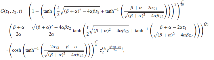 \begin{align}&G(z_1, z_2, t)=\left(1-\left(\tanh\left(\frac{t}2 \sqrt{(\beta+\alpha)^2 - 4\alpha\beta z_2}+\tanh^{-1}\left(\frac{\beta+\alpha-2\alpha z_1 }{\sqrt{(\beta+\alpha)^2 - 4\alpha\beta z_2}} \right)\right)\right)^2\right)^{\!\frac{\eta^*}{2\alpha}}\nonumber \\&\quad\cdot \left(\frac{\beta + \alpha}{2\alpha}-\frac{\sqrt{(\beta+\alpha)^2 - 4\alpha\beta z_2} }{2\alpha}\tanh \left(\frac{t}2 \sqrt{(\beta+\alpha)^2 - 4\alpha\beta z_2} + \tanh^{-1}\left(\frac{ \beta+\alpha-2\alpha z_1}{\sqrt{(\beta+\alpha)^2 - 4\alpha\beta z_2}} \right) \right)\right)^{Q_0}\nonumber \\&\quad\cdot \left(\cosh \left(\tanh^{-1}\left(\frac{2\alpha z_1 - \beta - \alpha}{\sqrt{(\beta+\alpha)^2 - 4\alpha\beta z_2}} \right)\right)\right)^{\!\frac{\eta^*}{\alpha}}z_2^{D_0} e^{\frac{\eta^*(\beta-\alpha)}{2\alpha}t},\end{align}
where $Q_0$
and
$Q_0$
and $D_0$
are the active number in the system and the count of departures at time 0, respectively.
$D_0$
are the active number in the system and the count of departures at time 0, respectively.
Proof. We will show this through the method of characteristics. We can first observe through Lemma 2 that
 \begin{align*}\frac{\textrm{d}}{\textrm{d}t}{\mathbb{E}\!\left[z_1^{Q_t} z_2^{D_t}\right]}&={\mathbb{E}\!\left[(\eta^* + \alpha Q_t)(z_1-1)z_1^{Q_t}z_2^{D_t} + \beta Q_t \left(\frac{z_2}{z_1}-1\right)z_1^{Q_t}z_2^{D_t}\right]},\end{align*}
and so $G(z_1,z_2,t)$
is given by the following PDE:
$G(z_1,z_2,t)$
is given by the following PDE:
 \begin{align*}\frac{\partial}{\partial t} G(z_1,z_2,t)+\left(\alpha (z_1-z_1^2) + \beta (z_1-z_2)\right)\frac{\partial}{\partial z_1} G(z_1,z_2,t)&=\eta^* (z_1 - 1) G(z_1,z_2,t).\end{align*}
To simplify our analysis, we will instead solve for $\log(G(z_1,z_2,t))$
, which through the chain rule will be given by the solution to the PDE expressed as
$\log(G(z_1,z_2,t))$
, which through the chain rule will be given by the solution to the PDE expressed as
 \begin{align*}\frac{\partial}{\partial t} \log(G(z_1,z_2,t))+\left(\alpha (z_1-z_1^2) + \beta (z_1-z_2)\right)\frac{\partial}{\partial z_1} \log(G(z_1,z_2,t))&=\eta^* (z_1 - 1),\end{align*}
with initial condition $\log(G(z_1,z_2,0)) = \log(z_1^{Q_0}z_2^{D_0})$
. This gives us the characteristic equations as follows:
$\log(G(z_1,z_2,0)) = \log(z_1^{Q_0}z_2^{D_0})$
. This gives us the characteristic equations as follows:
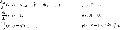 \begin{align*}\frac{\textrm{d}z_1}{\textrm{d}s}(r,s)&=\alpha (z_1-z_1^2) + \beta (z_1-z_2),&&z_1(r,0) = r,\\\frac{\textrm{d}t}{\textrm{d}s}(r,s)&=1,&&t(r,0) = 0,\\\frac{\textrm{d}g}{\textrm{d}s}(r,s)&=\eta^* ( z_1 - 1),&&g(r,0) = \log(r^{Q_0}z_2^{D_0}).\end{align*}
Solving the first two equations, we see that
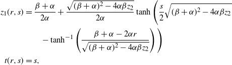 \begin{align*}z_1(r,s)&=\frac{\beta + \alpha}{2\alpha}+\frac{\sqrt{(\beta+\alpha)^2-4\alpha\beta z_2}}{2\alpha}\tanh\Bigg(\frac{s}{2} \sqrt{(\beta+\alpha)^2-4\alpha\beta z_2}\\&\qquad - \tanh^{-1}\left(\frac{\beta+\alpha-2\alpha r}{\sqrt{(\beta+\alpha)^2-4\alpha\beta z_2}}\right)\Bigg)\\t(r,s)&=s,\end{align*}
which allows us to solve for g(r, s). Using the solution to $z_1(r,s)$
, the ODE for g(r, s) is given by
$z_1(r,s)$
, the ODE for g(r, s) is given by
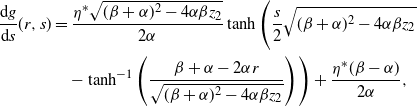 \begin{align*}\frac{\textrm{d}g}{\textrm{d}s}(r,s)&=\frac{\eta^*\sqrt{(\beta+\alpha)^2-4\alpha\beta z_2}}{2\alpha}\tanh\Bigg(\frac{s}{2} \sqrt{(\beta+\alpha)^2-4\alpha\beta z_2}\\&\quad-\tanh^{-1}\left(\frac{\beta+\alpha-2\alpha r}{\sqrt{(\beta+\alpha)^2-4\alpha\beta z_2}}\right)\Bigg)+\frac{\eta^*(\beta - \alpha)}{2\alpha},\end{align*}
which yields a solution of
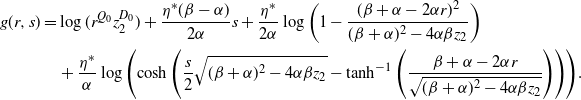 \begin{align*}g(r,s)&=\log(r^{Q_0} z_2^{D_0})+\frac{\eta^*(\beta-\alpha)}{2\alpha}s+\frac{\eta^*}{2\alpha}\log\left(1-\frac{(\beta+\alpha - 2\alpha r)^2}{(\beta+\alpha)^2-4\alpha\beta z_2}\right)\\&\quad+\frac{\eta^*}{\alpha}\log\left(\cosh\left(\frac{s}{2}\sqrt{(\beta+\alpha)^2 - 4\alpha\beta z_2}-\tanh^{-1}\left(\frac{\beta+\alpha-2\alpha r}{\sqrt{(\beta+\alpha)^2-4\alpha\beta z_2}}\right)\right)\right)\!.\end{align*}
Now, from these equations we can express the characteristic variables in terms of the original arguments as $s = t$
and
$s = t$
and
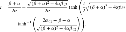 \begin{align*}r&=\frac{\beta+\alpha}{2\alpha}-\frac{\sqrt{(\beta+\alpha)^2 - 4\alpha\beta z_2} }{2\alpha}\tanh \Bigg(\frac{t}{2}\sqrt{(\beta+\alpha)^2-4\alpha\beta z_2}\\&\qquad -\tanh^{-1}\left(\frac{2\alpha z_1 -\beta-\alpha}{\sqrt{(\beta+\alpha)^2-4\alpha\beta z_2}}\right)\Bigg).\end{align*}
Then, by performing the substitution $G(z_1,z_2,t)=e^{g(r(z_1,z_2,t),s(z_1,z_2,t))}$
and simplifying, we achieve the stated result.
$G(z_1,z_2,t)=e^{g(r(z_1,z_2,t),s(z_1,z_2,t))}$
and simplifying, we achieve the stated result.
As another auxiliary result, in Proposition 12 we give the steady-state moment generating function for the 2-GESEP with exponentially distributed activity durations and deterministic batch sizes, meaning pairs of arrivals.
Proposition 12. Consider the following 2-GESEP: arrivals occur at rate $\eta_t(2) = \eta^* + \frac{\alpha}{2} Q_t(2)$
, where
$\eta_t(2) = \eta^* + \frac{\alpha}{2} Q_t(2)$
, where $Q_t(2)$
receives arrivals in batches of size 2. Each activity duration is independent and exponentially distributed with rate
$Q_t(2)$
receives arrivals in batches of size 2. Each activity duration is independent and exponentially distributed with rate $\beta > \alpha > 0$
. Then the steady-state moment generating function of
$\beta > \alpha > 0$
. Then the steady-state moment generating function of $Q_t(2)$
is given by
$Q_t(2)$
is given by
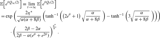 \begin{align}&{\mathbb{E}\!\left[e^{\theta Q_\infty (2)}\right]}\equiv\lim_{t\to\infty}{\mathbb{E}\!\left[e^{\theta Q_t (2)}\right]}\nonumber \\&=\exp \left(\frac{2\eta^*}{ \sqrt{\alpha (\alpha +8 \beta )}} \left( \tanh^{-1}\left(\left(2 e^\theta +1\right) \sqrt{\frac{\alpha }{\alpha +8 \beta }}\,\,\right)-\tanh ^{-1}\left(3 \sqrt{\frac{\alpha }{\alpha +8\beta }}\,\,\right)\right)\right)\nonumber \\&\qquad \cdot \left(\frac{2\beta - 2\alpha}{2\beta - \alpha (e^\theta + e^{2\theta})}\right)^{\!\frac{\eta^*}{\alpha}}.\end{align}
Proof. Using Lemma 2, we see that the moment generating function will be given by the solution to
 \begin{align*}\frac{\textrm{d}}{\textrm{d}t}{\mathbb{E}\!\left[e^{\theta Q_t (2)}\right]}&={\mathbb{E}\!\left[\left(\eta^* + \frac{\alpha Q_t (2)}{2}\right)\left(e^{\theta ( Q_t (2)+2)}-e^{\theta Q_t (2)}\right)+\beta Q_t(2)\left(e^{\theta ( Q_t (2)-1)}-e^{\theta Q_t (2)}\right)\right]},\end{align*}
which can be equivalently expressed in PDE form as
 \begin{align*}\frac{\partial}{\partial t}\mathcal{M}_2(\theta, t)&=\eta^*\left(e^{2\theta} - 1\right)\mathcal{M}_2(\theta, t)+\left(\frac{\alpha}{2}\left(e^{2\theta} - 1\right)+\beta\left(e^{-\theta} - 1\right)\right)\frac{\partial}{\partial \theta}\mathcal{M}_2(\theta, t),\end{align*}
where $\mathcal{M}_2(\theta, t) = {\mathbb{E}\!\left[e^{\theta Q_t (2)}\right]}$
. To solve for the steady-state moment generating function we consider the ODE given by
$\mathcal{M}_2(\theta, t) = {\mathbb{E}\!\left[e^{\theta Q_t (2)}\right]}$
. To solve for the steady-state moment generating function we consider the ODE given by
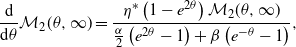 \begin{align*}\frac{\textrm{d}}{\textrm{d} \theta}\mathcal{M}_2(\theta, \infty)&=\frac{\eta^*\left(1 - e^{2\theta} \right)\mathcal{M}_2(\theta, \infty)}{\frac{\alpha}{2}\left(e^{2\theta} - 1\right)+\beta\left(e^{-\theta} - 1\right)},\end{align*}
with the initial condition that $\mathcal{M}_2(0, \infty) = 1$
. By taking the derivative of the expression in (23), we verify the result.
$\mathcal{M}_2(0, \infty) = 1$
. By taking the derivative of the expression in (23), we verify the result.
Appendix B. Exploring a hybrid self-exciting model
In the main body of the text we have defined the ESEP, a model that features arrivals that self-excite but only for a finite period of time. In contrast to the traditional Hawkes process models for self-excitement, in the ESEP the effect from one arrival does not decay through time but is fixed at a constant value for as long as it remains active. Thus, the ESEP features ephemeral but piecewise constant self-excitement, whereas the Hawkes process has eternal but ever decreasing self-excitement. One can note, though, that ephemeral self-excitement need not be piecewise constant. A model could feature both decay and down-jumps as ways of regulating its self-excitement. In this section of the appendix, we will consider such a model, specifically a Markovian one. To begin, let us now define the hybrid ephemerally self-exciting process (HESEP).
Definition 3. (Hybrid ephemerally self-exciting process.) Let $t \geq 0$
and suppose that
$t \geq 0$
and suppose that $\nu^* > 0$
,
$\nu^* > 0$
, $\alpha > 0$
,
$\alpha > 0$
, $\beta \geq 0$
, and
$\beta \geq 0$
, and $\mu \geq 0$
. Define
$\mu \geq 0$
. Define $\nu_t$
,
$\nu_t$
, $N_{t,\nu}$
, and
$N_{t,\nu}$
, and $Q_{t,\nu}$
such that the following hold:
$Q_{t,\nu}$
such that the following hold:
-
i.
$N_{t,\nu}$
is an arrival process driven by the intensity
$\nu_t$
; -
ii.
$Q_{t,\nu}$
is the number of arrivals from
$N_{t,\nu}$
that have not yet expired according to their i.i.d. Exp(
$\mu$
) activity durations; -
iii.
$\nu_t$
is governed by where
\begin{align*}\textrm{d}\nu_t=\beta(\nu^* - \nu_t)\textrm{d}t+\alpha \textrm{d}N_{t,\nu}-\frac{\nu_t - \nu^*}{Q_{t,\nu}}\textrm{d}D_{t,\nu},\end{align*}
$D_{t,\nu} = N_{t,\nu} - Q_{t,\nu}$
.


We say that the intensity–queue–counting-process triplet $(\nu_t, Q_{t,\nu}, N_{t,\nu})$
is a hybrid ephemerally self-exciting process (HESEP) with baseline intensity
$(\nu_t, Q_{t,\nu}, N_{t,\nu})$
is a hybrid ephemerally self-exciting process (HESEP) with baseline intensity $\nu^*$
, intensity jump size
$\nu^*$
, intensity jump size $\alpha$
, decay rate
$\alpha$
, decay rate $\beta$
, expiration rate
$\beta$
, expiration rate $\mu$
, and initial values
$\mu$
, and initial values $(\nu_0, Q_0^\nu, N_0^\nu)$
.
$(\nu_0, Q_0^\nu, N_0^\nu)$
.
By definition, one can view the HESEP as a hybrid between the ESEP and Hawkes process models. If $\beta = 0$
then we recover the ESEP; if
$\beta = 0$
then we recover the ESEP; if $\mu = 0$
then we recover the Hawkes process. Hence the dynamics are largely quite familiar: up-jumps of size
$\mu = 0$
then we recover the Hawkes process. Hence the dynamics are largely quite familiar: up-jumps of size $\alpha$
at each arrival, exponential decay between events at rate
$\alpha$
at each arrival, exponential decay between events at rate $\beta$
, and down-jumps upon each activity duration expiration. Perhaps the least intuitive part of this definition is the size of the down-jump, as this depends on the current levels of the intensity and the number of active exciters in the system. This draws inspiration from Markovian infinite-server queues. In an M/M/
$\beta$
, and down-jumps upon each activity duration expiration. Perhaps the least intuitive part of this definition is the size of the down-jump, as this depends on the current levels of the intensity and the number of active exciters in the system. This draws inspiration from Markovian infinite-server queues. In an M/M/ $\infty$
queue, all jobs currently in the system are equally likely to be the next to leave, regardless of the order in which they entered the system. Similarly, in the HESEP, each exciter in the system is equally likely to be the next to leave. Moreover, the down-jump size is the same regardless of which exciter is the next to leave. When the expiration of an activity duration means that there are no longer any presently active exciters, by definition the intensity will return to the baseline value. One can note that this down-jump size is actually always bounded below by 0, since the intensity decays down towards the baseline
$\infty$
queue, all jobs currently in the system are equally likely to be the next to leave, regardless of the order in which they entered the system. Similarly, in the HESEP, each exciter in the system is equally likely to be the next to leave. Moreover, the down-jump size is the same regardless of which exciter is the next to leave. When the expiration of an activity duration means that there are no longer any presently active exciters, by definition the intensity will return to the baseline value. One can note that this down-jump size is actually always bounded below by 0, since the intensity decays down towards the baseline $\nu^*$
, and is bounded above by
$\nu^*$
, and is bounded above by $\alpha$
, since
$\alpha$
, since $\nu_t - \nu^* \leq \alpha Q_{t,\nu}$
because each arrival increases
$\nu_t - \nu^* \leq \alpha Q_{t,\nu}$
because each arrival increases $\nu_t$
by
$\nu_t$
by $\alpha$
before it decays. As a quick interesting fact regarding this process, in Proposition 13 we show that the size of a down-jump,
$\alpha$
before it decays. As a quick interesting fact regarding this process, in Proposition 13 we show that the size of a down-jump, $(\nu_t - \nu^*)/Q_{t,\nu}$
, does not itself have down-jumps.
$(\nu_t - \nu^*)/Q_{t,\nu}$
, does not itself have down-jumps.
Proposition 13. Let $\phi_t = \frac{\nu_t - \nu^*}{Q_{t,\nu}}$
be the size of a down-jump occurring at time
$\phi_t = \frac{\nu_t - \nu^*}{Q_{t,\nu}}$
be the size of a down-jump occurring at time $t \geq 0$
. Suppose that
$t \geq 0$
. Suppose that $b \geq a \geq 0$
is such that
$b \geq a \geq 0$
is such that $Q_{t,\nu}$
is positive for all
$Q_{t,\nu}$
is positive for all $t \in [a,b]$
. Then
$t \in [a,b]$
. Then $\phi_t$
has no downward jumps on
$\phi_t$
has no downward jumps on $[a,b]$
.
$[a,b]$
.
Proof. Suppose that [a, b] is such an interval; then for $t \in [a,b]$
we note that
$t \in [a,b]$
we note that
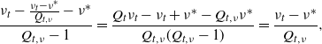 \begin{align*}\frac{\nu_t - \frac{\nu_t - \nu^*}{Q_{t,\nu}} - \nu^*}{Q_{t,\nu} - 1}=\frac{Q_t\nu_t - \nu_t + \nu^* - Q_{t,\nu}\nu^*}{Q_{t,\nu}(Q_{t,\nu} - 1)}=\frac{\nu_t - \nu^*}{Q_{t,\nu}},\end{align*}
and this is equal to $\phi_t$
.
$\phi_t$
.
B.1. Sandwiching the hybrid model
As one might expect for a so-called ‘hybrid’ model, the HESEP can be connected to the ESEP and the Hawkes process in many different ways. In Proposition 14, we show that one can actually sandwich this model between its two extremes. That is, we show that the means of the processes are equal when given the same parameters, whereas the variances are ordered with Hawkes as the smallest and ESEP as the largest.
Proposition 14. Let $\alpha > 0$
,
$\alpha > 0$
, $\beta > 0$
, and
$\beta > 0$
, and $\mu > 0$
be such that
$\mu > 0$
be such that $\mu + \beta > \alpha > 0$
. Additionally, let
$\mu + \beta > \alpha > 0$
. Additionally, let $\nu^* > 0$
. Let
$\nu^* > 0$
. Let $\nu_t$
be an HESEP with baseline intensity
$\nu_t$
be an HESEP with baseline intensity $\nu^*$
, intensity jump size
$\nu^*$
, intensity jump size $\alpha$
, decay rate
$\alpha$
, decay rate $\beta$
, and service rate
$\beta$
, and service rate $\mu$
. Similarly, let
$\mu$
. Similarly, let $\lambda_t$
be the intensity of a Hawkes process with baseline intensity
$\lambda_t$
be the intensity of a Hawkes process with baseline intensity $\nu^*$
, intensity jump
$\nu^*$
, intensity jump $\alpha$
, and decay rate
$\alpha$
, and decay rate $\mu + \beta$
. Finally, let
$\mu + \beta$
. Finally, let $\eta_t$
be the intensity of an ESEP with baseline intensity
$\eta_t$
be the intensity of an ESEP with baseline intensity $\nu^*$
, intensity jump
$\nu^*$
, intensity jump $\alpha$
, and service rate
$\alpha$
, and service rate $\mu + \beta$
. Then the means of these process intensities are all equal:
$\mu + \beta$
. Then the means of these process intensities are all equal:
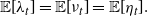 \begin{align}{\mathbb{E}\!\left[\lambda_t\right]} = {\mathbb{E}\!\left[\nu_t\right]} = {\mathbb{E}\!\left[\eta_t\right]}.\end{align}
Furthermore, the process variances are ordered as follows:
 \begin{align}{\textrm{Var}\left({\lambda_t}\right)} \leq {\textrm{Var}\left({\nu_t}\right)} \leq {\textrm{Var}\left({\eta_t}\right)}.\end{align}
Additionally, let $N_{t,\nu}$
,
$N_{t,\nu}$
, $N_{t,\lambda}$
, and
$N_{t,\lambda}$
, and $N_{t,\eta}$
be the counting processes of the HESEP, Hawkes process, and ESEP, respectively. Then the means of these counting processes are equal, i.e.
$N_{t,\eta}$
be the counting processes of the HESEP, Hawkes process, and ESEP, respectively. Then the means of these counting processes are equal, i.e.
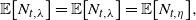 \begin{align}{\mathbb{E}\!\left[N_{t,\lambda}\right]} = {\mathbb{E}\!\left[N_{t,\lambda}\right]} = {\mathbb{E}\!\left[N_{t,\eta}\right]},\end{align}
and the variances of the counting processes are again ordered as follows:
 \begin{align}{\textrm{Var}\left({N_{t,\lambda}}\right)} \leq {\textrm{Var}\left({N_{t,\nu}}\right)} \leq {\textrm{Var}\left({N_{t,\eta}}\right)}.\end{align}
Finally, the covariances between the intensity and counting process pairs are likewise ordered as follows:
 \begin{align}{\textrm{Cov}[{\lambda_t, N_{t,\lambda}}]} \leq {\textrm{Cov}[{\nu_t, N_{t,\nu}}]} \leq {\textrm{Cov}[{\eta_t, N_{t,\eta}}]},\end{align}
where $t \geq 0$
and where all intensities have the same initial value.
$t \geq 0$
and where all intensities have the same initial value.
Proof. By a quick check of the differential equations for each mean, we can directly observe that ${\mathbb{E}\!\left[\nu_t\right]} = {\mathbb{E}\!\left[\eta_t\right]} = {\mathbb{E}\!\left[\lambda_t\right]}$
. To show the variance ordering we begin by considering the ODE for the second moment of
${\mathbb{E}\!\left[\nu_t\right]} = {\mathbb{E}\!\left[\eta_t\right]} = {\mathbb{E}\!\left[\lambda_t\right]}$
. To show the variance ordering we begin by considering the ODE for the second moment of $\nu_t$
:
$\nu_t$
:
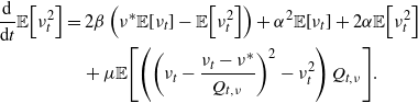 \begin{align*}\frac{\textrm{d}}{\textrm{d}t}{\mathbb{E}\!\left[\nu_t^2\right]}&=2\beta\left(\nu^* {\mathbb{E}\!\left[\nu_t\right]}-{\mathbb{E}\!\left[\nu_t^2\right]}\right)+\alpha^2 {\mathbb{E}\!\left[\nu_t\right]}+2\alpha {\mathbb{E}\!\left[\nu_t^2\right]}\\&\quad +\mu {\mathbb{E}\!\left[\left(\left(\nu_t - \frac{\nu_t - \nu^*}{Q_{t,\nu}}\right)^2 - \nu_t^2\right)Q_{t,\nu}\right]}.\end{align*}
Now, let us observe that
 \begin{align*}{\mathbb{E}\!\left[\left(\left(\nu_t - \frac{\nu_t - \nu^*}{Q_{t,\nu}}\right)^2 - \nu_t^2\right)Q_{t,\nu}\right]}&=2\left(\nu^* {\mathbb{E}\!\left[\nu_t\right]} - {\mathbb{E}\!\left[\nu_t^2\right]}\right) + {\mathbb{E}\!\left[\frac{(\nu_t - \nu^*)^2}{Q_{t,\nu}}\right]},\end{align*}
which follows from expanding the squared term. Because $\frac{(\nu_t - \nu^*)^2}{Q_{t,\nu}} \geq 0$
, this gives us that
$\frac{(\nu_t - \nu^*)^2}{Q_{t,\nu}} \geq 0$
, this gives us that
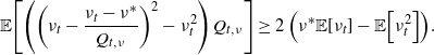 \begin{align}{\mathbb{E}\!\left[\left(\left(\nu_t - \frac{\nu_t - \nu^*}{Q_{t,\nu}}\right)^2 - \nu_t^2\right)Q_{t,\nu}\right]}&\geq 2\left(\nu^* {\mathbb{E}\!\left[\nu_t\right]} - {\mathbb{E}\!\left[\nu_t^2\right]}\right)\!.\end{align}
This inequality now allows us to directly compare $\frac{\textrm{d}}{\textrm{d}t}{\mathbb{E}\!\left[\nu_t^2\right]}$
to
$\frac{\textrm{d}}{\textrm{d}t}{\mathbb{E}\!\left[\nu_t^2\right]}$
to $\frac{\textrm{d}}{\textrm{d}t}{\mathbb{E}\!\left[\lambda_t^2\right]}$
and
$\frac{\textrm{d}}{\textrm{d}t}{\mathbb{E}\!\left[\lambda_t^2\right]}$
and $\frac{\textrm{d}}{\textrm{d}t}{\mathbb{E}\!\left[\eta_t^2\right]}$
. First, we can use (29) to see that
$\frac{\textrm{d}}{\textrm{d}t}{\mathbb{E}\!\left[\eta_t^2\right]}$
. First, we can use (29) to see that
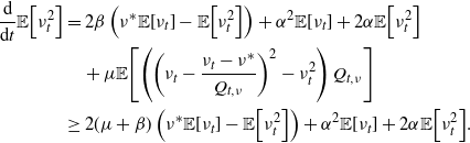 \begin{align*}\frac{\textrm{d}}{\textrm{d}t}{\mathbb{E}\!\left[\nu_t^2\right]}&=2\beta\left(\nu^* {\mathbb{E}\!\left[\nu_t\right]}-{\mathbb{E}\!\left[\nu_t^2\right]}\right)+\alpha^2 {\mathbb{E}\!\left[\nu_t\right]}+2\alpha {\mathbb{E}\!\left[\nu_t^2\right]}\\&\quad +\mu {\mathbb{E}\!\left[\left(\left(\nu_t - \frac{\nu_t - \nu^*}{Q_{t,\nu}}\right)^2 - \nu_t^2\right)Q_{t,\nu}\right]}\\&\geq 2(\mu+\beta)\left(\nu^* {\mathbb{E}\!\left[\nu_t\right]}-{\mathbb{E}\!\left[\nu_t^2\right]}\right)+\alpha^2 {\mathbb{E}\!\left[\nu_t\right]}+2\alpha {\mathbb{E}\!\left[\nu_t^2\right]}.\end{align*}
Because we have already shown that ${\mathbb{E}\!\left[\lambda_t\right]} = {\mathbb{E}\!\left[\nu_t\right]}$
, we see that
${\mathbb{E}\!\left[\lambda_t\right]} = {\mathbb{E}\!\left[\nu_t\right]}$
, we see that $\frac{\textrm{d}}{\textrm{d}t}{\mathbb{E}\!\left[\lambda_t^2\right]} \leq \frac{\textrm{d}}{\textrm{d}t}{\mathbb{E}\!\left[\nu_t^2\right]}$
when evaluated at the same point, and thus by Lemma 3,
$\frac{\textrm{d}}{\textrm{d}t}{\mathbb{E}\!\left[\lambda_t^2\right]} \leq \frac{\textrm{d}}{\textrm{d}t}{\mathbb{E}\!\left[\nu_t^2\right]}$
when evaluated at the same point, and thus by Lemma 3, ${\textrm{Var}\left({\lambda_t}\right)} \leq {\textrm{Var}\left({\nu_t}\right)}$
. By analogous arguments for
${\textrm{Var}\left({\lambda_t}\right)} \leq {\textrm{Var}\left({\nu_t}\right)}$
. By analogous arguments for $\eta_t$
, we achieve the stated result. For the counting process means, we can now observe that all the differential equations are such that
$\eta_t$
, we achieve the stated result. For the counting process means, we can now observe that all the differential equations are such that
 \begin{align*}\frac{\textrm{d}}{\textrm{d}t}{\mathbb{E}\!\left[N_{t,\lambda}\right]} = {\mathbb{E}\!\left[\lambda_t\right]}= \frac{\textrm{d}}{\textrm{d}t}{\mathbb{E}\!\left[N_{t,\nu}\right]} = {\mathbb{E}\!\left[\nu_t\right]}= \frac{\textrm{d}}{\textrm{d}t}{\mathbb{E}\!\left[N_{t,\eta}\right]} = {\mathbb{E}\!\left[\eta_t\right]}.\end{align*}
We assume that all counting processes start at 0, and thus we have that the counting process means are equal throughout time. This also implies that the products of means, ${\mathbb{E}\!\left[\lambda_t\right]}{\mathbb{E}\!\left[N_{t,\lambda}\right]}$
,
${\mathbb{E}\!\left[\lambda_t\right]}{\mathbb{E}\!\left[N_{t,\lambda}\right]}$
, ${\mathbb{E}\!\left[\nu_t\right]}{\mathbb{E}\!\left[N_{t,\nu}\right]}$
, and
${\mathbb{E}\!\left[\nu_t\right]}{\mathbb{E}\!\left[N_{t,\nu}\right]}$
, and ${\mathbb{E}\!\left[\eta_t\right]}{\mathbb{E}\!\left[N_{t,\eta}\right]}$
, are equal. Hence, to show the ordering of the covariances, we will focus solely on the expectations of the products. This differential equation is given by
${\mathbb{E}\!\left[\eta_t\right]}{\mathbb{E}\!\left[N_{t,\eta}\right]}$
, are equal. Hence, to show the ordering of the covariances, we will focus solely on the expectations of the products. This differential equation is given by
 \begin{align*}\frac{\textrm{d}}{\textrm{d}t}{\mathbb{E}\!\left[\nu_t N_{t,\nu}\right]}&=-(\mu + \beta - \alpha){\mathbb{E}\!\left[\nu_t N_{t,\nu}\right]} + (\mu+\beta)\nu^*{\mathbb{E}\!\left[N_{t,\nu}\right]} + \alpha{\mathbb{E}\!\left[\nu_t\right]} + {\mathbb{E}\!\left[\nu_t^2\right]},\end{align*}
and we can note that the coefficients are the same for each of the processes. Not including the function for which we want to solve, ${\mathbb{E}\!\left[\nu_t N_{t,\nu}\right]}$
, we can also observe that every function is equivalent across the processes, apart from the second moments of the intensities. We have shown that these second moments are in fact ordered, and therefore we arrive at the stated ordering of the covariances. Finally, we observe that the differential equation for the second moment of each counting process is of the form
${\mathbb{E}\!\left[\nu_t N_{t,\nu}\right]}$
, we can also observe that every function is equivalent across the processes, apart from the second moments of the intensities. We have shown that these second moments are in fact ordered, and therefore we arrive at the stated ordering of the covariances. Finally, we observe that the differential equation for the second moment of each counting process is of the form
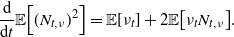 \begin{align*}\frac{\textrm{d}}{\textrm{d}t}{\mathbb{E}\!\left[(N_{t,\nu})^2\right]} = {\mathbb{E}\!\left[\nu_t\right]} + 2{\mathbb{E}\!\left[\nu_t N_{t,\nu}\right]}.\end{align*}
From the ordering of the covariances and the equivalences of the means, we can conclude the proof.
As a simple consequence of Proposition 14, we can note that because the Hawkes process is over-dispersed, i.e. its variance is larger than its mean, so too are the ESEP and HESEP. These bounds on the variance of the HESEP are not only useful for comparison but also practical for the study of the HESEP itself, as the system of differential equations for the variance obtained via the infinitesimal generator is not closed.
B.2. Strong convergence of the HESEP counting process
In the final three subsections on the analysis of the HESEP, we obtain a trio of limiting results. We begin with the almost sure convergence of the ratio of the HESEP counting process and time, which is an elementary renewal result in the style of [Reference Blackwell9] or [Reference Lindvall45], for example. However, in contrast to the context of such works, we can bound the mean and variance of the HESEP via the ESEP, and we are instead interested solely in establishing the convergence, as we will obtain additional results by consequence. Using these expressions for the first two moments, the proof of Theorem 3 follows standard approaches using the Borel–Cantelli lemma. In Corollary 1 we use this renewal result to find a strong law of large numbers for the dependent and non-identically distributed inter-arrival times of the HESEP by way of the continuous mapping theorem, which is another standard technique.
Theorem 3. Let $(\nu_t, Q_{t,\nu}, N_{t,\nu})$
be an HESEP with baseline intensity
$(\nu_t, Q_{t,\nu}, N_{t,\nu})$
be an HESEP with baseline intensity $\nu^*$
, intensity jump
$\nu^*$
, intensity jump $\alpha > 0$
, intensity decay rate
$\alpha > 0$
, intensity decay rate $\beta \geq 0$
, and rate of exponentially distributed service
$\beta \geq 0$
, and rate of exponentially distributed service $\mu \geq 0$
, where
$\mu \geq 0$
, where $\mu + \beta > \alpha$
. Then
$\mu + \beta > \alpha$
. Then
 \begin{align} \frac{N_{t,\nu}}{t}\stackrel{\textrm{a.s.}}{\longrightarrow }\nu_\infty\end{align}
as $t \to \infty$
, where
$t \to \infty$
, where $\nu_\infty = \frac{(\mu + \beta) \nu^*}{\mu + \beta - \alpha}$
.
$\nu_\infty = \frac{(\mu + \beta) \nu^*}{\mu + \beta - \alpha}$
.
Proof. We will show this through use of the Borel–Cantelli lemma. Let $\epsilon > 0$
be arbitrary, and define the event
$\epsilon > 0$
be arbitrary, and define the event $E_s$
for
$E_s$
for $s \in \mathbb{N}$
as
$s \in \mathbb{N}$
as
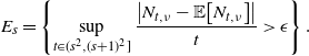 \begin{align*}E_s = \left\{\sup_{t \in (s^2, (s+1)^2]} \frac{\big|N_{t,\nu} - {\mathbb{E}\!\left[N_{t,\nu}\right]}\big|}{t} > \epsilon \right\}.\end{align*}
We now note that $N_{t,\nu} - {\mathbb{E}\!\left[N_{t,\nu}\right]}$
is a martingale by definition, and so
$N_{t,\nu} - {\mathbb{E}\!\left[N_{t,\nu}\right]}$
is a martingale by definition, and so $|N_{t,\nu} - {\mathbb{E}\!\left[N_{t,\nu}\right]}|$
is a sub-martingale. Additionally, we can observe that
$|N_{t,\nu} - {\mathbb{E}\!\left[N_{t,\nu}\right]}|$
is a sub-martingale. Additionally, we can observe that
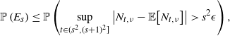 \begin{align*}\mathbb{P}\left( E_s \right)\leq \mathbb{P}\left( \sup_{t \in (s^2, (s+1)^2]} \big|N_{t,\nu} - {\mathbb{E}\!\left[N_{t,\nu}\right]}\big| > s^2 \epsilon \right),\end{align*}
because $s^2 \leq t$
for any t. By Doob’s martingale inequality, we have
$s^2 \leq t$
for any t. By Doob’s martingale inequality, we have
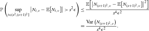 \begin{align*}\mathbb{P}\left( \sup_{t \in (s^2, (s+1)^2]} \big|N_{t,\nu} - {\mathbb{E}\!\left[N_{t,\nu}\right]}\big| > s^2 \epsilon \right)&\leq \frac{{\mathbb{E}\!\left[\big|N_{(s+1)^2,\nu} - {\mathbb{E}\!\left[N_{(s+1)^2,\nu}\right]}\big|^2\right]}}{s^4 \epsilon^2}\\&=\frac{{\textrm{Var}\left({N_{(s+1)^2,\nu}}\right)}}{s^4 \epsilon^2}.\end{align*}
From Proposition 14, we note that the variance of an HESEP counting process with baseline intensity $\nu^*$
, intensity jump size
$\nu^*$
, intensity jump size $\alpha$
, decay rate
$\alpha$
, decay rate $\beta$
, and service rate
$\beta$
, and service rate $\mu$
is bounded above by the variance of an ESEP counting process with baseline
$\mu$
is bounded above by the variance of an ESEP counting process with baseline $\nu^*$
, jump size
$\nu^*$
, jump size $\alpha$
, and service rate
$\alpha$
, and service rate $\mu + \beta$
. Using the explicit form of the ESEP counting process variance as computed through Lemma 2, we have the bound
$\mu + \beta$
. Using the explicit form of the ESEP counting process variance as computed through Lemma 2, we have the bound
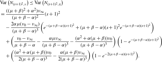 \begin{align*}&{\textrm{Var}\left({N_{(s+1)^2,\nu}}\right)}\leq {\textrm{Var}\left({N_{(s+1)^2,\eta}}\right)}\\&=\frac{((\mu+\beta)^2+ \alpha^2)\nu_\infty}{(\mu+\beta-\alpha)^2}(s+1)^2\\&\quad-\frac{2\alpha\mu(\nu_0 - \nu_\infty)}{(\mu+\beta-\alpha)^3}\bigg(e^{-(\mu+\beta - \alpha)(s+1)^2}+ (\mu+\beta-\alpha)(s+1)^2e^{-(\mu+\beta -\alpha)(s+1)^2}\bigg)\\&\quad+\left(\frac{\nu_0 - \nu_\infty}{\mu+\beta-\alpha}-\frac{\alpha\mu \nu_\infty}{(\mu+\beta-\alpha)^3}-\frac{(\alpha^2 + \alpha(\mu+\beta))\nu_0}{(\mu+\beta-\alpha)^3}\right)\bigg(1- e^{-(\mu+\beta-\alpha)(s+1)^2}\bigg)\\&\quad+\left(\frac{(\alpha^2 + \alpha(\mu+\beta))\nu_0}{2(\mu+\beta-\alpha)^3} - \frac{\alpha (\mu+\beta)\nu_\infty}{2(\mu+\beta-\alpha)^3}\right)\left(1 - e^{-2(\mu+\beta-\alpha)(s+1)^2}\right)\!.\end{align*}
Together, this implies that $\mathbb{P}\left( E_s \right) \in O\left(\frac{1}{s^2}\right)$
. Therefore
$\mathbb{P}\left( E_s \right) \in O\left(\frac{1}{s^2}\right)$
. Therefore $\sum_{s = 0}^\infty \mathbb{P}\left( E_s \right) < \infty$
, and so by the Borel–Cantelli lemma,
$\sum_{s = 0}^\infty \mathbb{P}\left( E_s \right) < \infty$
, and so by the Borel–Cantelli lemma,
 \begin{align*}\frac{\big|N_{t,\nu} - {\mathbb{E}\!\left[N_{t,\nu}\right]}\big|}{t} \stackrel{\textrm{a.s.}}{\longrightarrow } 0.\end{align*}
Since $\lim_{t \to \infty} \frac{{{\mathbb{E}}\left[N_{t,\nu}\right]}}{t} = \nu_\infty$
, this completes the proof.
$\lim_{t \to \infty} \frac{{{\mathbb{E}}\left[N_{t,\nu}\right]}}{t} = \nu_\infty$
, this completes the proof.
As an immediate consequence of this, we achieve a law of large numbers for the dependent inter-arrival times.
Corollary 1. Let $(\nu_t, Q_{t,\nu}, N_{t,\nu})$
be an HESEP counting process with baseline intensity
$(\nu_t, Q_{t,\nu}, N_{t,\nu})$
be an HESEP counting process with baseline intensity $\nu^* > 0$
, intensity jump
$\nu^* > 0$
, intensity jump $\alpha > 0$
, intensity decay rate
$\alpha > 0$
, intensity decay rate $\beta \geq 0$
, and rate of exponentially distributed service
$\beta \geq 0$
, and rate of exponentially distributed service $\mu \geq 0$
, where
$\mu \geq 0$
, where $\mu + \beta > \alpha$
. Further, let
$\mu + \beta > \alpha$
. Further, let $S_k^\nu$
denote the kth inter-arrival time for
$S_k^\nu$
denote the kth inter-arrival time for $k \in \mathbb{Z}^+$
. Then
$k \in \mathbb{Z}^+$
. Then
 \begin{align}\frac{1}{n}\sum_{k=1}^n S_k^\nu \stackrel{\textrm{a.s.}}{\longrightarrow } \frac{1}{\nu_\infty}\end{align}
as $n \to \infty$
, where
$n \to \infty$
, where $\nu_\infty = \frac{(\mu+\beta) \nu^*}{\mu+\beta - \alpha}$
.
$\nu_\infty = \frac{(\mu+\beta) \nu^*}{\mu+\beta - \alpha}$
.
Proof. Let $A_n^\nu$
denote the time of the nth arrival for each
$A_n^\nu$
denote the time of the nth arrival for each $n \in \mathbb{Z}^+$
, which is to say that
$n \in \mathbb{Z}^+$
, which is to say that $A_n^\nu = \sum_{k=1}^n S_k^\nu$
. Now, observe that the time of the most recent arrival up to time t,
$A_n^\nu = \sum_{k=1}^n S_k^\nu$
. Now, observe that the time of the most recent arrival up to time t, $A_{N_{t,\nu}}^\nu$
, can be bounded as
$A_{N_{t,\nu}}^\nu$
, can be bounded as
 \begin{align*}t - S_{N_{t,\nu} + 1}^\nu \leq A_{N_{t,\nu}}^\nu \leq t,\end{align*}
since if
 \begin{align*}t - S_{N_{t,\nu} + 1}^\nu > A_{N_{t,\nu}}^\nu,\end{align*}
then arrival $N_{t,\nu} + 1$
would have occurred before time t. We also note that because
$N_{t,\nu} + 1$
would have occurred before time t. We also note that because $\nu^* > 0$
, we have
$\nu^* > 0$
, we have $N_{t,\nu} \to \infty$
as
$N_{t,\nu} \to \infty$
as $t \to \infty$
, and this implies that
$t \to \infty$
, and this implies that
 \begin{align*}\frac{S_{N_{t,\nu} + 1}}{N_{t,\nu}} \stackrel{\textrm{a.s.}}{\longrightarrow } 0\end{align*}
as $t \to \infty$
. From Proposition 3 and the continuous mapping theorem, we know that
$t \to \infty$
. From Proposition 3 and the continuous mapping theorem, we know that
 \begin{align*}\frac{t}{N_{t,\nu}} \to \frac{1}{\nu_\infty}\end{align*}
and
 \begin{align*}\frac{t - S_{N_{t,\nu} + 1}}{N_{t,\nu}} \to \frac{1}{\nu_\infty}\end{align*}
almost surely. By the sandwiching of $A_{N_{t,\nu}}$
, this yields the stated result.
$A_{N_{t,\nu}}$
, this yields the stated result.
Because the Hawkes process and the ESEP are special cases of this hybrid model, we can note that both the renewal result and the law of large numbers apply directly to each.
Corollary 2. Let $(\lambda_t, N_{t,\lambda})$
be the intensity and count of a Hawkes process with baseline intensity
$(\lambda_t, N_{t,\lambda})$
be the intensity and count of a Hawkes process with baseline intensity $\lambda^* > 0$
, intensity jump
$\lambda^* > 0$
, intensity jump $\alpha > 0$
, and decay rate
$\alpha > 0$
, and decay rate $\beta > \alpha$
. Similarly, let
$\beta > \alpha$
. Similarly, let $(\eta_t, N_{t,\eta})$
be the intensity and counting process pair for an ESEP with baseline intensity
$(\eta_t, N_{t,\eta})$
be the intensity and counting process pair for an ESEP with baseline intensity $\nu^* > 0$
, intensity jump
$\nu^* > 0$
, intensity jump $\alpha > 0$
, and rate of exponentially distributed service
$\alpha > 0$
, and rate of exponentially distributed service $\mu > \alpha$
. Then, for
$\mu > \alpha$
. Then, for $S^\lambda_k$
and
$S^\lambda_k$
and $S^\eta_k$
as the kth inter-arrival times for the Hawkes process and the ESEP process, respectively, we have that
$S^\eta_k$
as the kth inter-arrival times for the Hawkes process and the ESEP process, respectively, we have that
 \begin{align}&\quad \frac{N_{t,\lambda}}{t}\stackrel{\textrm{a.s.}}{\longrightarrow }\lambda_\infty, \quad\frac{N_{t,\eta}}{t}\stackrel{\textrm{a.s.}}{\longrightarrow }\eta_\infty,\end{align}
and
 \begin{align}&\frac{1}{n}\sum_{k=1}^n S_k^\lambda \stackrel{\textrm{a.s.}}{\longrightarrow } \frac{1}{\lambda_\infty},&&\frac{1}{n}\sum_{k=1}^n S_k^\eta \stackrel{\textrm{a.s.}}{\longrightarrow } \frac{1}{\eta_\infty},\end{align}
where $\lambda_\infty = \frac{\beta \lambda^*}{\beta - \alpha}$
and
$\lambda_\infty = \frac{\beta \lambda^*}{\beta - \alpha}$
and $\eta_\infty = \frac{\mu \nu^*}{\mu - \alpha}$
.
$\eta_\infty = \frac{\mu \nu^*}{\mu - \alpha}$
.
B.3. Baseline fluid limit of the HESEP
In this subsection and in the sequel, we consider a baseline scaling of the HESEP. That is, we investigate limiting properties of the process as the baseline intensity grows large and the intensity and queue length are normalized in some fashion. To begin, we take the normalization as directly proportional to the baseline scaling, which is the fluid limit. The derivation of this is empowered by the following lemma, which allows us to make use of Taylor expansions.
Lemma 4. Suppose that for some $b > 0$
,
$b > 0$
, $ -b \leq z_n(t) \leq 0$
for all values of n. Then there exist constants
$ -b \leq z_n(t) \leq 0$
for all values of n. Then there exist constants $C_1$
and
$C_1$
and $C_2$
, where
$C_2$
, where $C_1 \leq C_2$
, which imply the following bounds for sufficiently large values of n:
$C_1 \leq C_2$
, which imply the following bounds for sufficiently large values of n:
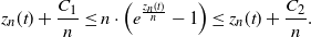 \begin{eqnarray}z_{n}(t) + \frac{C_1}{n} \leq n \cdot \left( e^{ \frac{ z_n(t) }{n} } - 1 \right) \leq z_{n}(t) + \frac{C_2}{n}.\end{eqnarray}
Proof. The proof follows from performing a second-order Taylor expansion for the exponential function and observing that since $z_n(t)$
lies in a compact interval, we can construct uniform lower and upper bounds for the exponential function.
$z_n(t)$
lies in a compact interval, we can construct uniform lower and upper bounds for the exponential function.
With this lemma in hand, we now proceed to finding the fluid limit in Theorem 4. In this case, we scale the baseline intensity by n, whereas we scale the intensity and the queue length by $\frac{1}{n}$
. As one would expect, we find that the fluid limit converges to the means of the intensity and queue.
$\frac{1}{n}$
. As one would expect, we find that the fluid limit converges to the means of the intensity and queue.
Theorem 4. For $n \in \mathbb{Z}$
, let the nth fluid-scaled HESEP
$n \in \mathbb{Z}$
, let the nth fluid-scaled HESEP $(\nu_t(n), Q_{t,\nu}(n))$
be defined so that the baseline intensity is
$(\nu_t(n), Q_{t,\nu}(n))$
be defined so that the baseline intensity is $n\nu^*$
, the intensity jump size is
$n\nu^*$
, the intensity jump size is $\alpha > 0$
, the intensity decay rate is
$\alpha > 0$
, the intensity decay rate is $\beta \geq 0$
, and the rate of exponentially distributed service is
$\beta \geq 0$
, and the rate of exponentially distributed service is $\mu > 0$
, where
$\mu > 0$
, where $\mu + \beta > \alpha$
. Then, for the scaled quantities
$\mu + \beta > \alpha$
. Then, for the scaled quantities
 \begin{align*}\left(\frac{\nu_{t,\nu}(n)}{n}, \frac{Q_{t,\nu}(n)}{n} \right),\end{align*}
the limit of the moment generating function,
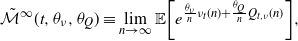 \begin{align}\tilde {\mathcal{M}}^{\infty}(t,\theta_{\nu},\theta_Q)\equiv \lim_{n \to \infty} {\mathbb{E}\!\left[e^{\frac{\theta_{\nu}}{n} \nu_t(n) + \frac{\theta_Q}{n} Q_{t,\nu}(n)} \right]} ,\end{align}
is given by
 \begin{align}\tilde {\mathcal{M}}^{\infty}(t,\theta_{\nu},\theta_Q)&=e^{\theta_\nu {\mathbb{E}\,\left[\nu_t\right]} + \theta_Q {\mathbb{E}\,\left[Q_{t,\nu}\right]}}\end{align}
for all $t \geq 0$
.
$t \geq 0$
.
Proof. The proof has two steps. The first step is to show that the limiting moment generating function converges to a PDE given by $\tilde{\mathcal{M}}^{\infty}$
using properties of the exponential function and Lemma 4. The second step is to solve this PDE using the method of characteristics. Finally, by the uniqueness of moment generating functions, we can assert that the random variables to which our limit converges are deterministic functions of time, which are also known as the fluid limit. We begin with the infinitesimal generator form, which is simplified through the linearity of expectation as
$\tilde{\mathcal{M}}^{\infty}$
using properties of the exponential function and Lemma 4. The second step is to solve this PDE using the method of characteristics. Finally, by the uniqueness of moment generating functions, we can assert that the random variables to which our limit converges are deterministic functions of time, which are also known as the fluid limit. We begin with the infinitesimal generator form, which is simplified through the linearity of expectation as
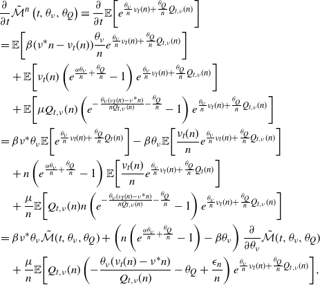 \begin{align*}&\frac{\partial}{\partial t} \tilde{\mathcal{M}}^n\left(t, \theta_\nu, \theta_Q\right)\equiv\frac{\partial }{\partial t} {\mathbb{E}\!\left[e^{\frac{\theta_{\nu}} {n} \nu_t(n) + \frac{\theta_Q }{n} Q_{t,\nu}(n) } \right]}\\&={\mathbb{E}\!\left[\beta (\nu^* n - \nu_t(n)) \frac{\theta_\nu}{n} e^{\frac{\theta_{\nu}} {n} \nu_t(n) + \frac{\theta_Q }{n} Q_{t,\nu}(n) } \right]}\\&\quad+{\mathbb{E}\!\left[\nu_t(n) \left( e^{\frac{\alpha\theta_\nu}{n} + \frac{\theta_Q}{n}} - 1\right) e^{\frac{\theta_{\nu}} {n} \nu_t(n) + \frac{\theta_Q }{n} Q_{t,\nu}(n) } \right]}\\&\quad+{\mathbb{E}\!\left[\mu Q_{t,\nu}(n) \left( e^{-\frac{\theta_\nu(\nu_t(n) - \nu^*n)}{n Q_{t,\nu}(n)} - \frac{\theta_Q }{n}} - 1 \right) e^{\frac{\theta_{\nu}} {n} \nu_t(n) + \frac{\theta_Q }{n} Q_{t,\nu}(n) } \right]}\\&=\beta \nu^* \theta_\nu {\mathbb{E}\!\left[ e^{\frac{\theta_{\nu}} {n} \nu_t(n) + \frac{\theta_Q }{n} Q_t(n) } \right]}-\beta \theta_\nu{\mathbb{E}\!\left[ \frac{\nu_t(n)}{n} e^{\frac{\theta_{\nu}} {n} \nu_t(n) + \frac{\theta_Q }{n} Q_{t,\nu}(n) } \right]}\\&\quad+n\left( e^{\frac{\alpha\theta_\nu}{n} + \frac{\theta_Q}{n}} - 1\right){\mathbb{E}\!\left[\frac{\nu_t(n)}{n} e^{\frac{\theta_{\nu}} {n} \nu_t(n) + \frac{\theta_Q }{n} Q_t(n) } \right]}\\&\quad+\frac{\mu}{n}{\mathbb{E}\!\left[ Q_{t,\nu}(n) n\left( e^{-\frac{\theta_\nu(\nu_t(n) - \nu^*n)}{n Q_{t,\nu}(n)} - \frac{\theta_Q }{n}} - 1 \right) e^{\frac{\theta_{\nu}} {n} \nu_t(n) + \frac{\theta_Q }{n} Q_{t,\nu}(n) } \right]}\\&=\beta \nu^* \theta_\nu \tilde{\mathcal{M}}(t, \theta_\nu, \theta_Q)+\left(n\left( e^{\frac{\alpha\theta_\nu}{n} + \frac{\theta_Q}{n}} - 1\right)-\beta \theta_\nu\right)\frac{\partial}{\partial \theta_\nu} \tilde{\mathcal{M}}(t, \theta_\nu, \theta_Q)\\&\quad+\frac{\mu}{n}{\mathbb{E}\!\left[ Q_{t,\nu}(n) \left( -\frac{\theta_\nu(\nu_t(n) - \nu^*n)}{ Q_{t,\nu}(n)} - \theta_Q + \frac{\epsilon_n}{n} \right) e^{\frac{\theta_{\nu}} {n} \nu_t(n) + \frac{\theta_Q }{n} Q_{t,\nu}(n) } \right]},\end{align*}
where the last equality holds for sufficiently large n, with $\epsilon_n$
in some bounded interval as according to Lemma 4. Then, by rearranging further, we can see that in the limit this becomes
$\epsilon_n$
in some bounded interval as according to Lemma 4. Then, by rearranging further, we can see that in the limit this becomes
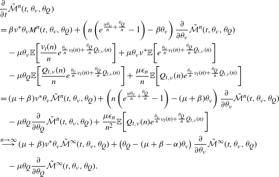 \begin{align*}&\frac{\partial}{\partial t} \tilde{\mathcal{M}}^n(t, \theta_\nu, \theta_Q)\\&=\beta \nu^* \theta_\nu M^n(t, \theta_\nu, \theta_Q)+\left(n\left( e^{\frac{\alpha\theta_\nu}{n} + \frac{\theta_Q}{n}} - 1\right)-\beta \theta_\nu\right)\frac{\partial}{\partial \theta_\nu} \tilde{\mathcal{M}}^n(t, \theta_\nu, \theta_Q)\\&\quad-\mu \theta_\nu{\mathbb{E}\!\left[ \frac{\nu_t(n)}{n} e^{\frac{\theta_{\nu}} {n} \nu_t(n) + \frac{\theta_Q }{n} Q_{t,\nu}(n) } \right]}+\mu \theta_\nu \nu^*{\mathbb{E}\!\left[ e^{\frac{\theta_{\nu}} {n} \nu_t(n) + \frac{\theta_Q }{n} Q_{t,\nu}(n) } \right]}\\&\quad-\mu \theta_Q{\mathbb{E}\!\left[ \frac{Q_{t,\nu}(n)}{n} e^{\frac{\theta_{\nu}} {n} \nu_t(n) + \frac{\theta_Q }{n} Q_{t,\nu}(n) } \right]}+\frac{\mu \epsilon_n}{n}{\mathbb{E}\!\left[ Q_{t,\nu}(n) e^{\frac{\theta_{\nu}} {n} \nu_t(n) + \frac{\theta_Q }{n} Q_{t,\nu}(n) } \right]}\\&=(\mu + \beta) \nu^* \theta_\nu \tilde{\mathcal{M}}^n(t, \theta_\nu, \theta_Q)+\left(n\left( e^{\frac{\alpha\theta_\nu}{n} + \frac{\theta_Q}{n}} - 1\right)-(\mu + \beta) \theta_\nu\right)\frac{\partial}{\partial \theta_\nu} \tilde{\mathcal{M}}^n(t, \theta_\nu, \theta_Q)\\&\quad-\mu \theta_Q\frac{\partial}{\partial \theta_Q} \tilde{\mathcal{M}}^n(t, \theta_\nu, \theta_Q)+\frac{\mu \epsilon_n}{n^2}{\mathbb{E}\!\left[ Q_{t,\nu}(n) e^{\frac{\theta_{\nu}} {n} \nu_t(n) + \frac{\theta_Q }{n} Q_{t,\nu}(n) } \right]}\\&\stackrel{n \to \infty}{\longrightarrow}(\mu + \beta) \nu^* \theta_\nu \tilde{\mathcal{M}}^\infty(t, \theta_\nu, \theta_Q)+\left(\theta_Q-(\mu + \beta - \alpha) \theta_\nu\right)\frac{\partial}{\partial \theta_\nu} \tilde{\mathcal{M}}^\infty(t, \theta_\nu, \theta_Q)\\&\quad-\mu \theta_Q\frac{\partial}{\partial \theta_Q} \tilde{\mathcal{M}}^\infty(t, \theta_\nu, \theta_Q).\end{align*}
We now solve this PDE for $\tilde{\mathcal{M}}^\infty(t, \theta_\nu, \theta_Q)$
through the method of characteristics. For simplicity’s sake we will instead use this procedure to solve for
$\tilde{\mathcal{M}}^\infty(t, \theta_\nu, \theta_Q)$
through the method of characteristics. For simplicity’s sake we will instead use this procedure to solve for $G(t,\theta_\nu,\theta_Q) = \log\left(\tilde{\mathcal{M}}^\infty(t, \theta_\nu, \theta_Q)\right)$
. This PDE is given by
$G(t,\theta_\nu,\theta_Q) = \log\left(\tilde{\mathcal{M}}^\infty(t, \theta_\nu, \theta_Q)\right)$
. This PDE is given by
 \begin{align*}(\mu + \beta) \nu^* \theta_\nu=\frac{\partial}{\partial t}G(t,\theta_\nu,\theta_Q)+\mu \theta_Q\frac{\partial}{\partial \theta_Q }G(t,\theta_\nu,\theta_Q)+\left((\mu + \beta - \alpha) \theta_\nu - \theta_Q\right)\frac{\partial}{\partial \theta_\nu }G(t,\theta_\nu,\theta_Q),\end{align*}
with boundary condition $G(0,\theta_\nu,\theta_Q) = \theta_Q Q_0 + \theta_\nu \nu_0$
. This corresponds to the following system of characteristic equations:
$G(0,\theta_\nu,\theta_Q) = \theta_Q Q_0 + \theta_\nu \nu_0$
. This corresponds to the following system of characteristic equations:
 \begin{align*}\frac{\textrm{d} \theta_Q}{\textrm{d}z}(x,y,z)&=\mu \theta_Q,&&\theta_Q(x,y,0) = x,\\\frac{\textrm{d} \theta_\nu}{\textrm{d}z}(x,y,z)&=(\mu + \beta - \alpha) \theta_\nu - \theta_Q,&&\theta_\nu(x,y,0) = y,\\\frac{\textrm{d} t}{\textrm{d}z}(x,y,z)&=1,&&t(x,y,0) = 0,\\\frac{\textrm{d} g}{\textrm{d}z}(x,y,z)&=(\mu + \beta) \nu^* \theta_\nu=(\mu+\beta-\alpha)\nu_\infty \theta_\nu,&&g(x,y,0) = x Q_0 + y \nu_0.\end{align*}
If $\beta \ne \alpha$
, the solutions to these initial value problems are given by the following:
$\beta \ne \alpha$
, the solutions to these initial value problems are given by the following:
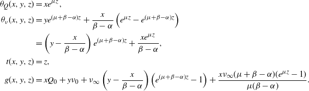 \begin{align*} \theta_Q(x,y,z)&=x e^{\mu z},\\ \theta_\nu(x,y,z)&=y e^{(\mu+\beta-\alpha)z}+\frac{x}{\beta-\alpha}\left(e^{\mu z} - e^{(\mu+\beta-\alpha)z}\right)\\&=\left( y - \frac{x}{\beta - \alpha}\right)e^{(\mu + \beta - \alpha)z}+\frac{x e^{\mu z}}{\beta-\alpha},\\ t(x,y,z)&=z,\\g(x,y,z)&=x Q_0 + y \nu_0+\nu_\infty \left( y - \frac{x}{\beta - \alpha}\right)\left( e^{(\mu + \beta - \alpha)z} - 1 \right)+\frac{x \nu_\infty (\mu+\beta -\alpha) (e^{\mu z}-1)}{\mu(\beta-\alpha)}.\end{align*}
Now we can solve for the characteristic variables in terms of the original variables and find $x=\theta_Q e^{-\mu t}$
,
$x=\theta_Q e^{-\mu t}$
,
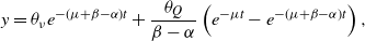 \begin{align*}y=\theta_\nu e^{-(\mu+\beta-\alpha)t}+\frac{\theta_Q}{\beta-\alpha}\left(e^{-\mu t} - e^{-(\mu+\beta-\alpha)t}\right),\end{align*}
and $z=t$
, so this gives a PDE solution of
$z=t$
, so this gives a PDE solution of
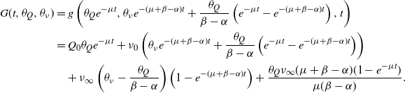 \begin{align*}G(t,\theta_Q, \theta_\nu)&=g\left(\theta_Q e^{-\mu t},\theta_\nu e^{-(\mu+\beta-\alpha)t} + \frac{\theta_Q}{\beta-\alpha}\left(e^{-\mu t} - e^{-(\mu+\beta-\alpha)t}\right),t\right)\\&=Q_0\theta_Q e^{-\mu t}+\nu_0\left(\theta_\nu e^{-(\mu+\beta-\alpha)t} + \frac{\theta_Q}{\beta-\alpha}\left(e^{-\mu t} - e^{-(\mu+\beta-\alpha)t}\right)\right)\\&\quad+\nu_\infty\left(\theta_\nu - \frac{\theta_Q}{\beta-\alpha}\right)\left( 1 - e^{-(\mu+\beta-\alpha)t} \right)+\frac{\theta_Q \nu_\infty (\mu+\beta -\alpha) (1-e^{-\mu t})}{\mu(\beta-\alpha)}.\end{align*}
If instead $\beta = \alpha$
, the solutions to the characteristic ODEs are as follows:
$\beta = \alpha$
, the solutions to the characteristic ODEs are as follows:
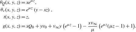 \begin{align*} \theta_Q(x,y,z)&=x e^{\mu z},\\ \theta_\nu(x,y,z)&=e^{\mu z} \left( y - x z \right),\\ t(x,y,z)&=z,\\g(x,y,z)&=x Q_0 + y \nu_0+\nu_\infty y \left( e^{\mu z} - 1 \right)-\frac{x \nu_\infty}{\mu} \left(e^{\mu z}(\mu z - 1) + 1\right)\!.\end{align*}
This makes our expressions for the characteristic variables $x=\theta_Q e^{-\mu t}$
,
$x=\theta_Q e^{-\mu t}$
, $y=\theta_\nu e^{-\mu t} + \theta_Q t e^{-\mu t}$
, and
$y=\theta_\nu e^{-\mu t} + \theta_Q t e^{-\mu t}$
, and $z=t$
. This leads to the PDE solution
$z=t$
. This leads to the PDE solution
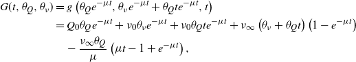 \begin{align*}G(t,\theta_Q, \theta_\nu)&=g\left(\theta_Q e^{-\mu t},\theta_\nu e^{-\mu t} + \theta_Q t e^{-\mu t},t\right)\\&=Q_0 \theta_Q e^{-\mu t}+\nu_0 \theta_\nu e^{-\mu t}+\nu_0 \theta_Q t e^{-\mu t}+\nu_\infty \left( \theta_\nu + \theta_Q t \right) \left( 1 - e^{-\mu t} \right)\\&\quad-\frac{ \nu_\infty \theta_Q }{\mu} \left(\mu t - 1 + e^{-\mu t}\right),\end{align*}
and we can observe that each of these cases simplifies to the corresponding means of the queue and the intensity, which yields the stated result.
B.4. Baseline diffusion limit of the HESEP
Now, to consider a diffusion limit, we still scale the baseline intensity by n, but we scale the process intensity and the queue length by $\frac{1}{\sqrt{n}}$
instead. More specifically, we scale the centered versions of the processes by
$\frac{1}{\sqrt{n}}$
instead. More specifically, we scale the centered versions of the processes by $\frac{1}{\sqrt{n}}$
. While we can make use of some of the techniques used for the fluid limit in Theorem 4, the diffusion scaling also involves second-order terms. It is challenging to calculate such quantities for the HESEP. Thus, we will use the same idea to bound the quantities above and below via
$\frac{1}{\sqrt{n}}$
. While we can make use of some of the techniques used for the fluid limit in Theorem 4, the diffusion scaling also involves second-order terms. It is challenging to calculate such quantities for the HESEP. Thus, we will use the same idea to bound the quantities above and below via
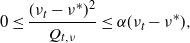 \begin{align}0 \leq \frac{(\nu_t - \nu^*)^2}{Q_{t,\nu}} \leq \alpha (\nu_t - \nu^*),\end{align}
which follows from our previously discussed bounds on the down-jump size. By doing so, we create upper and lower bounds for the true diffusion limit of the HESEP. To facilitate a variety of approximations that fit within these bounds, we introduce the parameter $\gamma \in [0,1]$
, with
$\gamma \in [0,1]$
, with $\gamma = 0$
corresponding to the lower bound and
$\gamma = 0$
corresponding to the lower bound and $\gamma = 1$
to the upper.
$\gamma = 1$
to the upper.
Theorem 5. For $n \in \mathbb{Z}$
, let the nth diffusion-scaled HESEP
$n \in \mathbb{Z}$
, let the nth diffusion-scaled HESEP $(\nu_t(n), Q_{t,\nu}(n))$
be defined so that the baseline intensity is
$(\nu_t(n), Q_{t,\nu}(n))$
be defined so that the baseline intensity is $n\nu^*$
, the intensity jump size is
$n\nu^*$
, the intensity jump size is $\alpha > 0$
, the intensity decay rate is
$\alpha > 0$
, the intensity decay rate is $\beta \geq 0$
, and the rate of exponentially distributed service is
$\beta \geq 0$
, and the rate of exponentially distributed service is $\mu > 0$
, where
$\mu > 0$
, where $\mu + \beta > \alpha$
. For the scaled quantities
$\mu + \beta > \alpha$
. For the scaled quantities $\left(\frac{\nu_t(n)}{\sqrt{n}}, \frac{Q_{t,\nu}(n)}{\sqrt{n}} \right)$
, let
$\left(\frac{\nu_t(n)}{\sqrt{n}}, \frac{Q_{t,\nu}(n)}{\sqrt{n}} \right)$
, let $\hat{\mathcal{M}}^{\infty}(t,\theta_{\nu},\theta_Q)$
be defined by
$\hat{\mathcal{M}}^{\infty}(t,\theta_{\nu},\theta_Q)$
be defined by
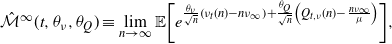 \begin{align}\hat{\mathcal{M}}^{\infty}(t,\theta_{\nu},\theta_Q)&\equiv\lim_{n \to \infty} {\mathbb{E}\!\left[e^{\frac{\theta_{\nu}} {\sqrt{n}} \left( \nu_t(n) - n\nu_\infty \right)+ \frac{\theta_Q }{\sqrt{n}} \left( Q_{t,\nu}(n) - \frac{n\nu_\infty}{\mu } \right) } \right]},\end{align}
if the limit converges. Then for $\beta \neq \alpha$
, this is bounded above and below by
$\beta \neq \alpha$
, this is bounded above and below by $\mathcal{B}_0(t,\theta_{\nu},\theta_Q) \leq \hat{\mathcal{M}}^{\infty}(t,\theta_{\nu},\theta_Q) \leq \mathcal{B}_1(t,\theta_{\nu},\theta_Q)$
, where
$\mathcal{B}_0(t,\theta_{\nu},\theta_Q) \leq \hat{\mathcal{M}}^{\infty}(t,\theta_{\nu},\theta_Q) \leq \mathcal{B}_1(t,\theta_{\nu},\theta_Q)$
, where $\mathcal{B}_\gamma(t,\theta_{\nu},\theta_Q)$
is given by
$\mathcal{B}_\gamma(t,\theta_{\nu},\theta_Q)$
is given by
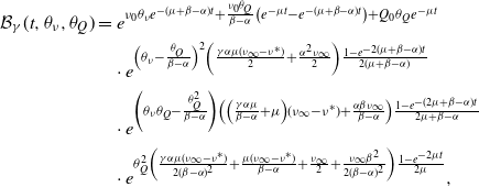 \begin{align}\mathcal{B}_\gamma(t,\theta_{\nu},\theta_Q)&=\nonumber e^{\nu_0\theta_\nu e^{-(\mu+\beta-\alpha)t} + \frac{\nu_0\theta_Q}{\beta-\alpha}\left(e^{-\mu t} - e^{-(\mu+\beta-\alpha)t}\right)+Q_0 \theta_Q e^{-\mu t}}\\\nonumber &\quad\cdot e^{\left(\theta_\nu - \frac{\theta_Q}{\beta - \alpha}\right)^2\left(\frac{\gamma \alpha \mu (\nu_\infty - \nu^*) }{2}+\frac{\alpha^2 \nu_\infty }{2 }\right)\frac{1 - e^{-2(\mu + \beta - \alpha)t}}{2(\mu + \beta - \alpha)}}\\&\quad\cdot e^{\left(\theta_\nu\theta_Q - \frac{\theta_Q^2}{\beta - \alpha}\right)\left(\left(\frac{\gamma \alpha\mu}{\beta-\alpha}+\mu\right)(\nu_\infty - \nu^*)+\frac{\alpha \beta \nu_\infty}{\beta-\alpha}\right)\frac{1-e^{-(2\mu + \beta-\alpha)t}}{2\mu+\beta-\alpha}}\nonumber \\&\quad\cdot e^{\theta_Q^2\left(\frac{\gamma \alpha \mu (\nu_\infty- \nu^*) }{2(\beta-\alpha)^2}+\frac{\mu(\nu_\infty - \nu^*) }{\beta-\alpha}+\frac{\nu_\infty }{2}+\frac{\nu_\infty \beta^2 }{2(\beta - \alpha)^2}\right)\frac{1 - e^{-2\mu t}}{2\mu}},\end{align}
whereas if $\beta = \alpha$
, it is instead
$\beta = \alpha$
, it is instead
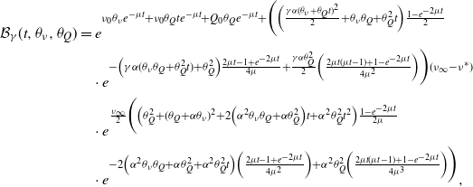 \begin{align}\mathcal{B}_\gamma(t,\theta_{\nu},\theta_Q)&=\nonumber e^{\nu_0 \theta_\nu e^{-\mu t} + \nu_0 \theta_Q t e^{- \mu t}+Q_0 \theta_Q e^{-\mu t}+\bigg(\left(\frac{\gamma \alpha (\theta_\nu + \theta_Q t)^2}{2} + \theta_\nu \theta_Q + \theta_Q^2 t\right) \frac{1 - e^{-2\mu t}}{2}}\\&\quad\cdot e^{-\left(\gamma \alpha (\theta_\nu \theta_Q + \theta_Q^2 t) + \theta_Q^2 \right) \frac{2\mu t - 1 + e^{-2\mu t} }{4 \mu}+\frac{\gamma \alpha \theta_Q^2}{2}\left(\frac{2\mu t(\mu t-1)+1 - e^{-2\mu t}}{4 \mu^2}\right)\bigg) (\nu_\infty - \nu^*)}\nonumber \\&\quad\cdot e^{\frac{\nu_\infty }{2 }\bigg(\left(\theta_Q^2 + (\theta_Q + \alpha \theta_\nu)^2+2\left(\alpha^2 \theta_\nu \theta_Q + \alpha \theta_Q^2 \right) t+\alpha^2 \theta_Q^2 t^2\right) \frac{1 - e^{-2\mu t}}{2\mu}}\nonumber \\&\quad\cdot e^{-2 \left(\alpha^2 \theta_\nu \theta_Q + \alpha \theta_Q^2 + \alpha^2 \theta_Q^2 t\right)\left(\frac{2\mu t - 1 + e^{-2\mu t} }{4 \mu^2}\right)+\alpha^2 \theta_Q^2 \left( \frac{ 2\mu t(\mu t-1) +1 - e^{-2\mu t}}{4 \mu^3} \right)\bigg)},\end{align}
for $\gamma \in [0,1]$
with
$\gamma \in [0,1]$
with $t \geq 0$
and
$t \geq 0$
and $\nu_\infty = \frac{(\mu + \beta)\nu^*}{\mu+\beta-\alpha}$
.
$\nu_\infty = \frac{(\mu + \beta)\nu^*}{\mu+\beta-\alpha}$
.
Proof. We begin by bounding the quantity $Q_{t,\nu}(n) \left(\frac{\nu_t(n) - n\nu^*}{Q_{t,\nu}(n)}\right)^2$
above and below by observing
$Q_{t,\nu}(n) \left(\frac{\nu_t(n) - n\nu^*}{Q_{t,\nu}(n)}\right)^2$
above and below by observing
 \begin{align*}0\leq Q_{t,\nu}(n) \left(\frac{\nu_t(n) - n\nu^*}{Q_{t,\nu}(n)}\right)^2=(\nu_t(n) - n\nu^*)\left(\frac{\nu_t(n) - n\nu^*}{Q_{t,\nu}(n)}\right)\leq \alpha (\nu_t(n) - n\nu^*).\end{align*}
To consolidate the development of the two bounds into one approach, we introduce the extra parameter $\gamma \in \{0,1\}$
and replace
$\gamma \in \{0,1\}$
and replace
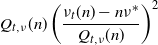 \begin{align*}Q_{t,\nu}(n) \left(\frac{\nu_t(n) - n\nu^*}{Q_{t,\nu}(n)}\right)^2\end{align*}
by $\gamma \alpha (\nu_t(n) - n\nu^*)$
in the following diffusion limit derivation. In this notation,
$\gamma \alpha (\nu_t(n) - n\nu^*)$
in the following diffusion limit derivation. In this notation, $\gamma = 0$
yields the lower bound and
$\gamma = 0$
yields the lower bound and $\gamma = 1$
the upper. These two cases share the same start—identifying the moment generating function form of the pre-limit object. By Lemma 2, this is
$\gamma = 1$
the upper. These two cases share the same start—identifying the moment generating function form of the pre-limit object. By Lemma 2, this is
 \begin{align*}&\frac{\partial}{\partial t}\hat{\mathcal{M}}^n(\theta_\nu, \theta_Q, t)=\frac{\partial}{\partial t}{\mathbb{E}\!\left[e^{\theta_\nu \left(\frac{\nu_t(n) - n \nu_\infty}{\sqrt{n}}\right) + \theta_Q \left(\frac{Q_{t,\nu}(n) - \frac{n \nu_\infty}{\mu}}{\sqrt{n}}\right)}\right]}\\&={\mathbb{E}\!\left[\nu_t(n)\left(e^{\frac{\alpha\theta_\nu + \theta_Q}{\sqrt{n}}} - 1 \right)e^{\theta_\nu \left(\frac{\nu_t(n) - n \nu_\infty}{\sqrt{n}}\right) + \theta_Q \left(\frac{Q_{t,\nu}(n) - \frac{n \nu_\infty}{\mu}}{\sqrt{n}}\right)}\right]}\\&\quad+{\mathbb{E}\!\left[\mu Q_{t,\nu}(n)\left(e^{-\frac{\theta_\nu}{\sqrt{n}}\left(\frac{\nu_t(n)-n\nu^*}{Q_{t,\nu}(n)}\right) - \frac{\theta_Q}{\sqrt{n}}} - 1 \right)e^{\theta_\nu \left(\frac{\nu_t(n) - n \nu_\infty}{\sqrt{n}}\right) + \theta_Q \left(\frac{Q_{t,\nu}(n) - \frac{n \nu_\infty}{\mu}}{\sqrt{n}}\right)}\right]}\\&\quad+{\mathbb{E}\!\left[\frac{\beta \theta_\nu}{\sqrt{n}}\left(n\nu^* - \nu_t(n)\right)e^{\theta_\nu \left(\frac{\nu_t(n) - n \nu_\infty}{\sqrt{n}}\right) + \theta_Q \left(\frac{Q_{t,\nu}(n) - \frac{n \nu_\infty}{\mu}}{\sqrt{n}}\right)}\right]}.\end{align*}
As a first step, we simplify this expression through the linearity of expectation. Moving deterministic terms outside of the expectation and rescaling, we have
 \begin{align*}&\frac{\partial}{\partial t}\hat{\mathcal{M}}^n(\theta_\nu, \theta_Q, t)=\sqrt{n}\left(e^{\frac{\alpha\theta_\nu + \theta_Q}{\sqrt{n}}} - 1 \right){\mathbb{E}\!\left[\frac{\nu_t(n)}{\sqrt{n}}e^{\theta_\nu \left(\frac{\nu_t(n) - n \nu_\infty}{\sqrt{n}}\right) + \theta_Q \left(\frac{Q_{t,\nu}(n) - \frac{n \nu_\infty}{\mu}}{\sqrt{n}}\right)}\right]}\\&\quad+{\mathbb{E}\!\left[\mu Q_{t,\nu}(n)\left(e^{-\frac{\theta_\nu}{\sqrt{n}}\left(\frac{\nu_t(n)-n\nu^*}{Q_{t,\nu}(n)}\right) - \frac{\theta_Q}{\sqrt{n}}} - 1 \right)e^{\theta_\nu \left(\frac{\nu_t(n) - n \nu_\infty}{\sqrt{n}}\right) + \theta_Q \left(\frac{Q_{t,\nu}(n) - \frac{n \nu_\infty}{\mu}}{\sqrt{n}}\right)}\right]}\\&\quad+\beta \theta_\nu \nu^* \sqrt{n} {\mathbb{E}\!\left[ e^{\theta_\nu \left(\frac{\nu_t(n) - n \nu_\infty}{\sqrt{n}}\right) + \theta_Q \left(\frac{Q_{t,\nu}(n) - \frac{n \nu_\infty}{\mu}}{\sqrt{n}}\right)}\right]}\\&\quad-\beta \theta_\nu {\mathbb{E}\!\left[\frac{\nu_t(n)}{\sqrt{n}}e^{\theta_\nu \left(\frac{\nu_t(n) - n \nu_\infty}{\sqrt{n}}\right) + \theta_Q \left(\frac{Q_{t,\nu}(n) - \frac{n \nu_\infty}{\mu}}{\sqrt{n}}\right)}\right]}.\end{align*}
For the terms on the first, third, and fourth lines in the right-hand side of the above equation, we are able to re-express the expectation in terms of the moment generating function or its derivatives. For the first and second lines, we perform Taylor expansions and truncate terms from the third order and above. This yields
 \begin{align*}&\frac{\partial}{\partial t}\hat{\mathcal{M}}^n(\theta_\nu, \theta_Q, t)=\left(\alpha\theta_\nu + \theta_Q + \frac{(\alpha\theta_\nu + \theta_Q)^2}{2 \sqrt{n}} + O\left(\frac{1}{n}\right) \right)\Bigg( \frac{\partial}{\partial \theta_\nu}\hat{\mathcal{M}}^n(\theta_\nu, \theta_Q, t)\\&\quad+ \nu_\infty\sqrt{n} \hat{\mathcal{M}}^n(\theta_\nu, \theta_Q, t) \Bigg)+\mathbb{E}\Bigg[\mu Q_{t,\nu}(n)\Bigg( -\frac{\theta_\nu}{\sqrt{n}}\left(\frac{\nu_t(n)-n\nu^*}{Q_{t,\nu}(n)}\right) - \frac{\theta_Q}{\sqrt{n}}\\&\quad+ \frac{1}{2n}\left(\theta_\nu\left(\frac{\nu_t(n)-n\nu^*}{Q_{t,\nu}(n)}\right) + \theta_Q\right)^2 + O\left(n^{-\frac{3}{2}}\right) \Bigg)e^{\theta_\nu \left(\frac{\nu_t(n) - n \nu_\infty}{\sqrt{n}}\right) + \theta_Q \left(\frac{Q_{t,\nu}(n) - \frac{n \nu_\infty}{\mu}}{\sqrt{n}}\right)}\Bigg]\\&\quad+\beta \theta_\nu \nu^* \sqrt{n} \hat{\mathcal{M}}^n(\theta_\nu, \theta_Q, t)-\beta \theta_\nu \left( \frac{\partial}{\partial \theta_\nu}\hat{\mathcal{M}}^n(\theta_\nu, \theta_Q, t) + \nu_\infty\sqrt{n} \hat{\mathcal{M}}^n(\theta_\nu, \theta_Q, t) \right)\!.\end{align*}
We now begin distributing and combining like terms through linearity of expectation. Moreover, we distribute within the expectation on the second line and cancel $Q_{t,\nu}(n)$
across the numerator and denominator where possible, obtaining
$Q_{t,\nu}(n)$
across the numerator and denominator where possible, obtaining
 \begin{align*}&\frac{\partial}{\partial t}\hat{\mathcal{M}}^n(\theta_\nu, \theta_Q, t)=\left(\alpha\theta_\nu + \theta_Q + \frac{(\alpha\theta_\nu + \theta_Q)^2}{2 \sqrt{n}} - \beta \theta_\nu + O\left(\frac{1}{n}\right) \right)\Bigg( \frac{\partial}{\partial \theta_\nu}\hat{\mathcal{M}}^n(\theta_\nu, \theta_Q, t)\\&\quad+ \nu_\infty\sqrt{n} \hat{\mathcal{M}}^n(\theta_\nu, \theta_Q, t) \Bigg)-\mu\theta_\nu {\mathbb{E}\!\left[\frac{\nu_t(n)}{\sqrt{n}}e^{\theta_\nu \left(\frac{\nu_t(n) - n \nu_\infty}{\sqrt{n}}\right) + \theta_Q \left(\frac{Q_{t,\nu}(n) - \frac{n \nu_\infty}{\mu}}{\sqrt{n}}\right)}\right]}\\&\quad+\mu \theta_\nu \nu^* \sqrt{n} {\mathbb{E}\!\left[ e^{\theta_\nu \left(\frac{\nu_t(n) - n \nu_\infty}{\sqrt{n}}\right) + \theta_Q \left(\frac{Q_{t,\nu}(n) - \frac{n \nu_\infty}{\mu}}{\sqrt{n}}\right)}\right]}\\&\quad-\mu \theta_Q {\mathbb{E}\!\left[\frac{ Q_{t,\nu}(n)}{\sqrt{n}}e^{\theta_\nu \left(\frac{\nu_t(n) - n \nu_\infty}{\sqrt{n}}\right) + \theta_Q \left(\frac{Q_{t,\nu}(n) - \frac{n \nu_\infty}{\mu}}{\sqrt{n}}\right)}\right]}\\&\quad+ \frac{\mu\theta_\nu^2}{2n}{\mathbb{E}\!\left[ Q_{t,\nu}(n) \left(\frac{\nu_t(n)-n\nu^*}{Q_{t,\nu}(n)}\right)^2 e^{\theta_\nu \left(\frac{\nu_t(n) - n \nu_\infty}{\sqrt{n}}\right) + \theta_Q \left(\frac{Q_{t,\nu}(n) - \frac{n \nu_\infty}{\mu}}{\sqrt{n}}\right)}\right]}\end{align*}
 \begin{align*}&\quad+ \frac{\mu\theta_\nu\theta_Q}{\sqrt{n}}{\mathbb{E}\!\left[ \frac{\nu_t(n)}{\sqrt{n}}e^{\theta_\nu \left(\frac{\nu_t(n) - n \nu_\infty}{\sqrt{n}}\right) + \theta_Q \left(\frac{Q_{t,\nu}(n) - \frac{n \nu_\infty}{\mu}}{\sqrt{n}}\right)}\right]} \\[3pt]&\quad- \mu\theta_\nu\theta_Q \nu^* {\mathbb{E}\!\left[e^{\theta_\nu \left(\frac{\nu_t(n) - n \nu_\infty}{\sqrt{n}}\right) + \theta_Q \left(\frac{Q_{t,\nu}(n) - \frac{n \nu_\infty}{\mu}}{\sqrt{n}}\right)}\right]}\\[3pt]&\quad+ \frac{\mu \theta_Q^2}{2\sqrt{n}}{\mathbb{E}\!\left[ \frac{Q_{t,\nu}(n)}{\sqrt{n}}e^{\theta_\nu \left(\frac{\nu_t(n) - n \nu_\infty}{\sqrt{n}}\right) + \theta_Q \left(\frac{Q_{t,\nu}(n) - \frac{n \nu_\infty}{\mu}}{\sqrt{n}}\right)}\right]} \\[3pt]&\quad+ O\left(\frac{1}{n}\right){\mathbb{E}\!\left[\frac{Q_{t,\nu}(n)}{\sqrt{n}} e^{\theta_\nu \left(\frac{\nu_t(n) - n \nu_\infty}{\sqrt{n}}\right) + \theta_Q \left(\frac{Q_{t,\nu}(n) - \frac{n \nu_\infty}{\mu}}{\sqrt{n}}\right)}\right]}\\[3pt]&\quad+\beta \theta_\nu \nu^* \sqrt{n} \hat{\mathcal{M}}^n(\theta_\nu, \theta_Q, t).\end{align*}
For all remaining components of this equation that are still expressed in terms of the expectation, we substitute equivalent forms in terms of the moment generating function or its partial derivatives. Furthermore, we will now replace
 \begin{align*}Q_{t,\nu}(n) \left(\frac{\nu_t(n) - n\nu^*}{Q_{t,\nu}(n)}\right)^2\end{align*}
by $\gamma \alpha (\nu_t(n) - n\nu^*)$
inside the expectation and re-express the expectation in terms of the moment generating function accordingly. To denote that we have now made this replacement and changed the function, we add
$\gamma \alpha (\nu_t(n) - n\nu^*)$
inside the expectation and re-express the expectation in terms of the moment generating function accordingly. To denote that we have now made this replacement and changed the function, we add $\gamma$
as a subscript to the moment generating function, i.e.
$\gamma$
as a subscript to the moment generating function, i.e. $\hat{\mathcal{M}}_\gamma^n(\theta_\nu, \theta_Q, t)$
. We now have
$\hat{\mathcal{M}}_\gamma^n(\theta_\nu, \theta_Q, t)$
. We now have
 \begin{align*}&\frac{\partial}{\partial t}\hat{\mathcal{M}}_\gamma^n(\theta_\nu, \theta_Q, t)=\left(\alpha\theta_\nu + \theta_Q + \frac{(\alpha\theta_\nu + \theta_Q)^2}{2 \sqrt{n}} - \beta \theta_\nu + O\left(\frac{1}{n}\right) \right)\Bigg( \frac{\partial}{\partial \theta_\nu}\hat{\mathcal{M}}_\gamma^n(\theta_\nu, \theta_Q, t)\\[3pt]&\quad+ \nu_\infty\sqrt{n} \hat{\mathcal{M}}_\gamma^n(\theta_\nu, \theta_Q, t) \Bigg)-\mu\theta_\nu \left( \frac{\partial}{\partial \theta_\nu}\hat{\mathcal{M}}_\gamma^n(\theta_\nu, \theta_Q, t) + \nu_\infty\sqrt{n} \hat{\mathcal{M}}_\gamma^n(\theta_\nu, \theta_Q, t) \right)\\[3pt]&\quad+\mu \theta_\nu \nu^* \sqrt{n} \hat{\mathcal{M}}_\gamma^n(\theta_\nu, \theta_Q, t)-\mu \theta_Q \left( \frac{\partial}{\partial \theta_Q}\hat{\mathcal{M}}_\gamma^n(\theta_\nu, \theta_Q, t)+\frac{\nu_\infty\sqrt{n}}{\mu} \hat{\mathcal{M}}_\gamma^n(\theta_\nu, \theta_Q, t) \right)\\[3pt]&\quad+ \frac{\gamma \alpha \mu\theta_\nu^2}{2\sqrt{n}}\left( \frac{\partial}{\partial \theta_\nu}\hat{\mathcal{M}}_\gamma^n(\theta_\nu, \theta_Q, t) + \nu_\infty\sqrt{n} \hat{\mathcal{M}}_\gamma^n(\theta_\nu, \theta_Q, t) \right)- \frac{\gamma \alpha \mu \nu^* \theta_\nu^2}{2}\hat{\mathcal{M}}_\gamma^n(\theta_\nu, \theta_Q, t)\\[3pt]&\quad+ \frac{\mu\theta_\nu\theta_Q}{\sqrt{n}}\left( \frac{\partial}{\partial \theta_\nu}\hat{\mathcal{M}}_\gamma^n(\theta_\nu, \theta_Q, t) + \nu_\infty\sqrt{n} \hat{\mathcal{M}}_\gamma^n(\theta_\nu, \theta_Q, t) \right)- \mu\theta_\nu\theta_Q \nu^* \hat{\mathcal{M}}_\gamma^n(\theta_\nu, \theta_Q, t)\\[3pt]&\quad+ \frac{\mu \theta_Q^2}{2\sqrt{n}}\left( \frac{\partial}{\partial \theta_Q}\hat{\mathcal{M}}_\gamma^n(\theta_\nu, \theta_Q, t) + \frac{\nu_\infty\sqrt{n}}{\mu} \hat{\mathcal{M}}_\gamma^n(\theta_\nu, \theta_Q, t) \right) +\beta \theta_\nu \nu^* \sqrt{n} \hat{\mathcal{M}}_\gamma^n(\theta_\nu, \theta_Q, t)\\[3pt]&\quad+ O\left(\frac{1}{n}\right) \left( \frac{\partial}{\partial \theta_Q}\hat{\mathcal{M}}_\gamma^n(\theta_\nu, \theta_Q, t) + \frac{\nu_\infty\sqrt{n}}{\mu} \hat{\mathcal{M}}_\gamma^n(\theta_\nu, \theta_Q, t) \right)\!.\end{align*}
Before we find the limiting object, we first combine like terms of the moment generating function, consolidating coefficients and absorbing into $O({\cdot})$
notation where possible:
$O({\cdot})$
notation where possible:
 \begin{align*}&\frac{\partial}{\partial t}\hat{\mathcal{M}}_\gamma^n(\theta_\nu, \theta_Q, t)=\left( \theta_Q - (\mu + \beta - \alpha)\theta_\nu + O\left(\frac{1}{\sqrt{n}}\right) \right) \frac{\partial}{\partial \theta_\nu}\hat{\mathcal{M}}_\gamma^n(\theta_\nu, \theta_Q, t)\\&\quad-\left( \mu \theta_Q - O\left(\frac{1}{\sqrt{n}}\right) \right) \frac{\partial}{\partial \theta_Q}\hat{\mathcal{M}}_\gamma^n(\theta_\nu, \theta_Q, t)\Bigg(\frac{\gamma \alpha \mu(\nu_\infty - \nu^*) \theta_\nu^2}{2}+\mu\theta_\nu\theta_Q (\nu_\infty - \nu^*)\\&\quad+\frac{\theta_Q^2 \nu_\infty}{2}+\frac{(\alpha\theta_\nu + \theta_Q)^2\nu_\infty }{2 }+O\left(\frac{1}{\sqrt{n}}\right) \Bigg) \hat{\mathcal{M}}_\gamma^n(\theta_\nu, \theta_Q, t).\end{align*}
Taking the limit as $n \to \infty$
, we get
$n \to \infty$
, we get
 \begin{align*}&\frac{\partial}{\partial t}\hat{\mathcal{M}}_\gamma^\infty(\theta_\nu, \theta_Q, t)=\left( \theta_Q - (\mu + \beta - \alpha)\theta_\nu \right) \frac{\partial}{\partial \theta_\nu}\hat{\mathcal{M}}_\gamma^\infty(\theta_\nu, \theta_Q, t)- \mu \theta_Q \frac{\partial}{\partial \theta_Q}\hat{\mathcal{M}}_\gamma^\infty(\theta_\nu, \theta_Q, t)\\&\quad+\left(\frac{\gamma \alpha \mu(\nu_\infty - \nu^*) \theta_\nu^2}{2}+\mu\theta_\nu\theta_Q (\nu_\infty - \nu^*)+\frac{\theta_Q^2 \nu_\infty}{2}+\frac{(\alpha\theta_\nu + \theta_Q)^2\nu_\infty }{2 } \right) \hat{\mathcal{M}}_\gamma^\infty(\theta_\nu, \theta_Q, t).\end{align*}
We will now solve this limiting PDE through the method of characteristics. To simplify this approach, we let $G_\gamma(\theta_\nu, \theta_Q, t) = \log\left(\hat{\mathcal{M}}_\gamma^\infty(\theta_\nu, \theta_Q, t)\right)$
, which is the cumulant generating function. The resulting PDE for the cumulant generating function is then
$G_\gamma(\theta_\nu, \theta_Q, t) = \log\left(\hat{\mathcal{M}}_\gamma^\infty(\theta_\nu, \theta_Q, t)\right)$
, which is the cumulant generating function. The resulting PDE for the cumulant generating function is then
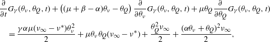 \begin{align*}&\frac{\partial}{\partial t}G_\gamma(\theta_\nu, \theta_Q, t)+\left( (\mu + \beta - \alpha)\theta_\nu - \theta_Q \right) \frac{\partial}{\partial \theta_\nu}G_\gamma(\theta_\nu, \theta_Q, t)+ \mu \theta_Q \frac{\partial}{\partial \theta_Q}G_\gamma(\theta_\nu, \theta_Q, t)\\&\quad=\frac{\gamma \alpha \mu(\nu_\infty - \nu^*) \theta_\nu^2}{2}+\mu\theta_\nu\theta_Q (\nu_\infty - \nu^*)+\frac{\theta_Q^2 \nu_\infty}{2}+\frac{(\alpha\theta_\nu + \theta_Q)^2\nu_\infty }{2 },\end{align*}
with initial condition $G_\gamma(\theta_\nu, \theta_Q, 0) = \theta_\nu \nu_0 + \theta_Q Q_0$
. Thus, the resulting system of characteristic equations is
$G_\gamma(\theta_\nu, \theta_Q, 0) = \theta_\nu \nu_0 + \theta_Q Q_0$
. Thus, the resulting system of characteristic equations is
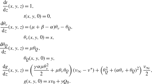 \begin{align*}\frac{\textrm{d}t}{\textrm{d}z}(x,y,z)&=1,\\&t(x,y,0) = 0,\\\frac{\textrm{d}\theta_\nu}{\textrm{d}z}(x,y,z)&=(\mu + \beta - \alpha)\theta_\nu - \theta_Q,\\&\theta_\nu(x,y,0) = x,\\\frac{\textrm{d}\theta_Q}{\textrm{d}z}(x,y,z)&=\mu \theta_Q,\\&\theta_Q(x,y,0) = y,\\\frac{\textrm{d}g}{\textrm{d}z}(x,y,z)&=\left(\frac{\gamma \alpha \mu \theta_\nu^2}{2}+\mu\theta_\nu\theta_Q \right) (\nu_\infty - \nu^*)+\left(\theta_Q^2 + (\alpha\theta_\nu + \theta_Q)^2\right) \frac{\nu_\infty }{2 },\\&g(x,y,0) = x \nu_0 + y Q_0.\end{align*}
Assuming $\beta \ne \alpha$
, we can solve these first three ODEs to find that
$\beta \ne \alpha$
, we can solve these first three ODEs to find that
 \begin{align*}t = z,\qquad \theta_Q = y e^{\mu z},\qquad \theta_\nu = \left(x - \frac{y}{\beta - \alpha}\right)e^{(\mu+\beta-\alpha)z} + \frac{y}{\beta-\alpha}e^{\mu z},\end{align*}
which we now use to solve the remaining equation. Rewriting the characteristic equation for g, we have
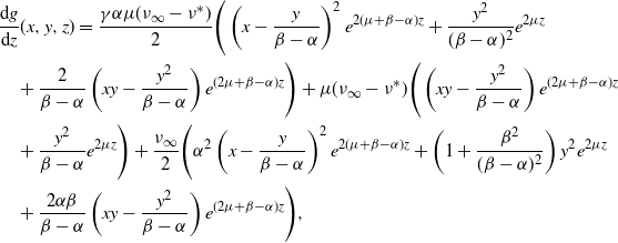 \begin{align*}&\frac{\textrm{d}g}{\textrm{d}z}(x,y,z)=\frac{\gamma \alpha \mu (\nu_\infty - \nu^*) }{2}\Bigg(\left(x - \frac{y}{\beta - \alpha}\right)^2e^{2(\mu+\beta-\alpha)z}+\frac{y^2}{(\beta-\alpha)^2}e^{2\mu z}\\&\quad+ \frac{2}{\beta-\alpha}\left( xy - \frac{y^2}{\beta - \alpha}\right)e^{(2\mu+\beta-\alpha)z}\Bigg)+\mu (\nu_\infty - \nu^*) \Bigg(\left(xy - \frac{y^2}{\beta - \alpha}\right)e^{(2\mu+\beta-\alpha)z}\\&\quad+ \frac{y^2}{\beta-\alpha}e^{2\mu z} \Bigg)+\frac{\nu_\infty }{2 }\Bigg(\alpha^2 \left(x - \frac{y}{\beta - \alpha}\right)^2 e^{2(\mu+\beta-\alpha)z}+\left(1 + \frac{\beta^2 }{(\beta-\alpha)^2} \right) y^2 e^{2\mu z}\\&\quad+\frac{2\alpha\beta}{\beta-\alpha}\left( xy-\frac{ y^2}{\beta - \alpha}\right)e^{(2\mu+\beta-\alpha)z}\Bigg),\end{align*}
and so by grouping coefficients of like exponential functions and then integrating with respect to z, we obtain the solution
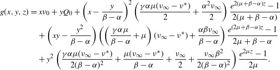 \begin{align*}g(x,y,z)&=x\nu_0 + y Q_0+\left(x - \frac{y}{\beta - \alpha}\right)^2\left(\frac{\gamma \alpha \mu (\nu_\infty - \nu^*) }{2}+\frac{\alpha^2 \nu_\infty }{2 }\right)\frac{e^{2(\mu + \beta - \alpha)z}-1}{2(\mu + \beta - \alpha)}\\&\quad+\left(xy - \frac{y^2}{\beta - \alpha}\right)\left(\left(\frac{\gamma \alpha\mu}{\beta-\alpha}+\mu\right)(\nu_\infty - \nu^*)+\frac{\alpha \beta \nu_\infty}{\beta-\alpha}\right)\frac{e^{(2\mu + \beta-\alpha)z}-1}{2\mu+\beta-\alpha}\\&\quad+y^2\left(\frac{\gamma \alpha \mu (\nu_\infty- \nu^*) }{2(\beta-\alpha)^2}+\frac{\mu(\nu_\infty - \nu^*) }{\beta-\alpha}+\frac{\nu_\infty }{2}+\frac{\nu_\infty \beta^2 }{2(\beta - \alpha)^2}\right)\frac{e^{2\mu z}-1}{2\mu}.\end{align*}
From the solutions to the characteristic equations, we can express each of x, y, and z in terms of the three cumulant generating function parameters:
 \begin{align*}z = t,\qquad y = \theta_Q e^{-\mu t},\qquad x = \theta_\nu e^{-(\mu+\beta-\alpha)t} + \frac{\theta_Q}{\beta-\alpha}\left(e^{-\mu t} - e^{-(\mu+\beta-\alpha)t}\right)\!.\end{align*}
Thus, we can solve for $G_\gamma(\theta_\nu, \theta_Q, t)$
via
$G_\gamma(\theta_\nu, \theta_Q, t)$
via
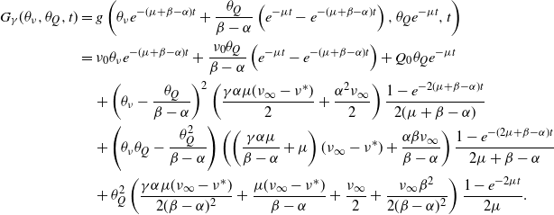 \begin{align*}G_\gamma(\theta_\nu, \theta_Q, t)&=g\left(\theta_\nu e^{-(\mu+\beta-\alpha)t} + \frac{\theta_Q}{\beta-\alpha}\left(e^{-\mu t} - e^{-(\mu+\beta-\alpha)t}\right), \theta_Q e^{-\mu t}, t \right)\\&=\nu_0\theta_\nu e^{-(\mu+\beta-\alpha)t} + \frac{\nu_0\theta_Q}{\beta-\alpha}\left(e^{-\mu t} - e^{-(\mu+\beta-\alpha)t}\right)+Q_0 \theta_Q e^{-\mu t}\\&\quad+\left(\theta_\nu - \frac{\theta_Q}{\beta - \alpha}\right)^2\left(\frac{\gamma \alpha \mu (\nu_\infty - \nu^*) }{2}+\frac{\alpha^2 \nu_\infty }{2 }\right)\frac{1 - e^{-2(\mu + \beta - \alpha)t}}{2(\mu + \beta - \alpha)}\\&\quad+\left(\theta_\nu\theta_Q - \frac{\theta_Q^2}{\beta - \alpha}\right)\left(\left(\frac{\gamma \alpha\mu}{\beta-\alpha}+\mu\right)(\nu_\infty - \nu^*)+\frac{\alpha \beta \nu_\infty}{\beta-\alpha}\right)\frac{1-e^{-(2\mu + \beta-\alpha)t}}{2\mu+\beta-\alpha}\\&\quad+\theta_Q^2\left(\frac{\gamma \alpha \mu (\nu_\infty- \nu^*) }{2(\beta-\alpha)^2}+\frac{\mu(\nu_\infty - \nu^*) }{\beta-\alpha}+\frac{\nu_\infty }{2}+\frac{\nu_\infty \beta^2 }{2(\beta - \alpha)^2}\right)\frac{1 - e^{-2\mu t}}{2\mu}.\end{align*}
By Lemma 3, we have that $\hat{\mathcal{M}}^\infty_0(\theta_\nu, \theta_Q, t) \leq \hat{\mathcal{M}}^\infty(\theta_\nu, \theta_Q, t) \leq \hat{\mathcal{M}}^\infty_1(\theta_\nu, \theta_Q, t)$
, and since
$\hat{\mathcal{M}}^\infty_0(\theta_\nu, \theta_Q, t) \leq \hat{\mathcal{M}}^\infty(\theta_\nu, \theta_Q, t) \leq \hat{\mathcal{M}}^\infty_1(\theta_\nu, \theta_Q, t)$
, and since $\hat{\mathcal{M}}^\infty_\gamma(\theta_\nu, \theta_Q, t) = e^{G_\gamma(\theta_\nu, \theta_Q, t)}$
, we have completed the proof of the joint moment generating function bounds when
$\hat{\mathcal{M}}^\infty_\gamma(\theta_\nu, \theta_Q, t) = e^{G_\gamma(\theta_\nu, \theta_Q, t)}$
, we have completed the proof of the joint moment generating function bounds when $\beta \ne \alpha$
. We now apply this to the two marginal generating functions by setting the opposite space parameter to 0. That is, for the intensity we let
$\beta \ne \alpha$
. We now apply this to the two marginal generating functions by setting the opposite space parameter to 0. That is, for the intensity we let $\theta_Q = 0$
, yielding
$\theta_Q = 0$
, yielding
 \begin{align*}\hat{\mathcal{M}}^\infty_\gamma(\theta_\nu, 0, t)&=\textrm{exp}\left(\nu_0\theta_\nu e^{-(\mu+\beta-\alpha)t}+\frac{\theta_\nu^2}2\left(\gamma \alpha \mu (\nu_\infty - \nu^*) + \alpha^2 \nu_\infty\right)\frac{1 - e^{-2(\mu + \beta - \alpha)t}}{2(\mu + \beta - \alpha)}\right),\end{align*}
whereas for the queue we take $\theta_\nu = 0$
and obtain
$\theta_\nu = 0$
and obtain
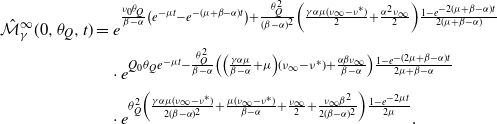 \begin{align*}{\hat{\mathcal{M}}^\infty_\gamma(0,\theta_Q, t)} & =e^{\frac{\nu_0\theta_Q}{\beta-\alpha}\left(e^{-\mu t} - e^{-(\mu+\beta-\alpha)t}\right)+\frac{\theta_Q^2}{(\beta - \alpha)^2}\left(\frac{\gamma \alpha \mu (\nu_\infty - \nu^*) }{2}+\frac{\alpha^2 \nu_\infty }{2 }\right)\frac{1 - e^{-2(\mu + \beta - \alpha)t}}{2(\mu + \beta - \alpha)}}\\&\quad\cdot e^{Q_0 \theta_Q e^{-\mu t}-\frac{\theta_Q^2}{\beta - \alpha}\left(\left(\frac{\gamma \alpha\mu}{\beta-\alpha}+\mu\right)(\nu_\infty - \nu^*)+\frac{\alpha \beta \nu_\infty}{\beta-\alpha}\right)\frac{1-e^{-(2\mu + \beta-\alpha)t}}{2\mu+\beta-\alpha}}\\&\quad\cdot e^{\theta_Q^2\left(\frac{\gamma \alpha \mu (\nu_\infty- \nu^*) }{2(\beta-\alpha)^2}+\frac{\mu(\nu_\infty - \nu^*) }{\beta-\alpha}+\frac{\nu_\infty }{2}+\frac{\nu_\infty \beta^2 }{2(\beta - \alpha)^2}\right)\frac{1 - e^{-2\mu t}}{2\mu}}.\end{align*}
Now if $\beta = \alpha$
, the solution to the characteristic ODE for
$\beta = \alpha$
, the solution to the characteristic ODE for $\theta_\nu$
is instead
$\theta_\nu$
is instead
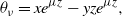 \begin{align*}\theta_\nu = x e^{\mu z} - y z e^{\mu z},\end{align*}
whereas the solutions for $\theta_Q$
and t are unchanged:
$\theta_Q$
and t are unchanged: $\theta_Q = y e^{\mu z}$
and
$\theta_Q = y e^{\mu z}$
and $t = z$
. This implies that the ODE for g is given by
$t = z$
. This implies that the ODE for g is given by
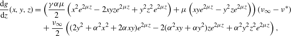 \begin{align*}\frac{\textrm{d}g}{\textrm{d}z}(x,y,z)&=\left(\frac{\gamma \alpha \mu }{2}\left( x^2 e^{2\mu z} - 2x y z e^{2\mu z} + y^2z^2 e^{2\mu z} \right)+\mu \left( x y e^{2\mu z} - y^2 z e^{2\mu z}\right)\right) (\nu_\infty - \nu^*)\\&\quad+\frac{\nu_\infty }{2 }\left((2y^2 + \alpha^2 x^2 + 2\alpha x y) e^{2\mu z}-2(\alpha^2 x y + \alpha y^2) z e^{2\mu z}+\alpha^2 y^2 z^2 e^{2\mu z}\right),\end{align*}
which yields a solution of
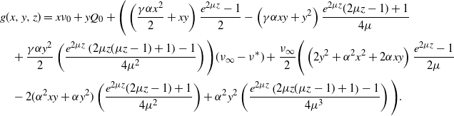 \begin{align*}&g(x,y,z)=x\nu_0+y Q_0+\Bigg(\left(\frac{\gamma \alpha x^2}{2} + x y\right) \frac{e^{2\mu z} - 1}{2}-\left(\gamma \alpha x y + y^2 \right) \frac{e^{2 \mu z}(2\mu z - 1) + 1 }{4 \mu}\\&\quad+\frac{\gamma \alpha y^2}{2}\left(\frac{e^{2\mu z}\left(2\mu z(\mu z-1)+1\right) - 1}{4 \mu^2}\right)\Bigg) (\nu_\infty - \nu^*)+\frac{\nu_\infty }{2 }\Bigg(\left(2y^2 + \alpha^2 x^2 + 2\alpha x y \right) \frac{e^{2\mu z} - 1}{2\mu}\\&\quad-2(\alpha^2 x y + \alpha y^2) \left(\frac{e^{2 \mu z}(2\mu z - 1) + 1 }{4 \mu^2}\right)+\alpha^2 y^2 \left( \frac{e^{2\mu z}\left(2\mu z(\mu z-1)+1\right) - 1}{4 \mu^3} \right)\Bigg).\end{align*}
In this case the inverse solutions are
 \begin{align*}z = t,\qquad y = \theta_Q e^{-\mu t},\qquad x = \theta_\nu e^{-\mu t} + \theta_Q t e^{- \mu t},\end{align*}
and so $G_\gamma(\theta_\nu, \theta_Q, t)$
is given by
$G_\gamma(\theta_\nu, \theta_Q, t)$
is given by
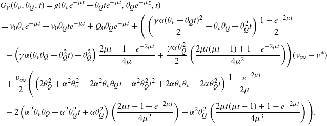 \begin{align*}&G_\gamma(\theta_\nu, \theta_Q, t)=g(\theta_\nu e^{-\mu t} + \theta_Q t e^{- \mu t}, \theta_Q e^{-\mu z}, t)\\&=\nu_0 \theta_\nu e^{-\mu t} + \nu_0 \theta_Q t e^{- \mu t}+Q_0 \theta_Q e^{-\mu t}+\Bigg(\left(\frac{\gamma \alpha (\theta_\nu + \theta_Q t)^2}{2} + \theta_\nu \theta_Q + \theta_Q^2 t\right) \frac{1 - e^{-2\mu t}}{2}\\&\ \ -\left(\gamma \alpha (\theta_\nu \theta_Q + \theta_Q^2 t) + \theta_Q^2 \right) \frac{2\mu t - 1 + e^{-2\mu t} }{4 \mu}+\frac{\gamma \alpha \theta_Q^2}{2}\left(\frac{2\mu t(\mu t-1)+1 - e^{-2\mu t}}{4 \mu^2}\right)\!\Bigg) (\nu_\infty - \nu^*)\\&\ \ +\frac{\nu_\infty }{2 }\Bigg(\left(2\theta_Q^2 + \alpha^2 \theta_\nu^2 + 2\alpha^2 \theta_\nu \theta_Q t + \alpha^2 \theta_Q^2 t^2 + 2 \alpha \theta_\nu \theta_\nu + 2\alpha \theta_Q^2 t \right) \frac{1 - e^{-2\mu t}}{2\mu}\\&\ \ -2 \left(\alpha^2 \theta_\nu \theta_Q + \alpha^2 \theta_Q^2 t + \alpha \theta_Q^2 \right) \left(\frac{2\mu t - 1 + e^{-2\mu t} }{4 \mu^2}\right)+\alpha^2 \theta_Q^2 \left( \frac{ 2\mu t(\mu t-1) +1 - e^{-2\mu t}}{4 \mu^3} \right)\Bigg).\end{align*}
By taking $\hat{\mathcal{M}}^\infty_\gamma(\theta_\nu, \theta_Q, t) = e^{G_\gamma(\theta_\nu, \theta_Q, t)}$
, we complete the proof.
$\hat{\mathcal{M}}^\infty_\gamma(\theta_\nu, \theta_Q, t) = e^{G_\gamma(\theta_\nu, \theta_Q, t)}$
, we complete the proof.
As a consequence of these diffusion approximations, we can give normally distributed approximations for the steady-state distributions of the HESEP intensity and queue length. These are stated below in Corollary 3, again in terms of $\gamma$
. One can note that the approximate intensity variance in (41) can be used to provide upper and lower bounds on the HESEP variance that may be tighter than the bounds from the ESEP and the Hawkes process in Proposition 14.
$\gamma$
. One can note that the approximate intensity variance in (41) can be used to provide upper and lower bounds on the HESEP variance that may be tighter than the bounds from the ESEP and the Hawkes process in Proposition 14.
Corollary 3. Let $(\nu_t, Q_{t,\nu})$
be an HESEP with baseline intensity
$(\nu_t, Q_{t,\nu})$
be an HESEP with baseline intensity $\nu^* > 0$
, intensity jump
$\nu^* > 0$
, intensity jump $\alpha > 0$
, decay rate
$\alpha > 0$
, decay rate $\beta > 0$
, and rate of exponential service
$\beta > 0$
, and rate of exponential service $\mu > 0$
, with
$\mu > 0$
, with $\mu + \beta > \alpha$
. Then the steady-state distributions of the processes
$\mu + \beta > \alpha$
. Then the steady-state distributions of the processes $\nu_t$
and
$\nu_t$
and $Q_{t,\nu}$
are approximated by the random variables
$Q_{t,\nu}$
are approximated by the random variables $X_\nu(\gamma) \sim N(\nu_\infty, \sigma^2_\nu(\gamma))$
and
$X_\nu(\gamma) \sim N(\nu_\infty, \sigma^2_\nu(\gamma))$
and $X_Q(\gamma) \sim N\big(\frac{\nu_\infty}{\mu}, \sigma^2_Q(\gamma)\big)$
, respectively, where
$X_Q(\gamma) \sim N\big(\frac{\nu_\infty}{\mu}, \sigma^2_Q(\gamma)\big)$
, respectively, where
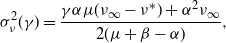 \begin{align}\sigma^2_\nu(\gamma)=\frac{\gamma \alpha \mu (\nu_\infty - \nu^*) + \alpha^2 \nu_\infty }{2(\mu+\beta-\alpha)},\end{align}
and if $\beta \ne \alpha$
then
$\beta \ne \alpha$
then
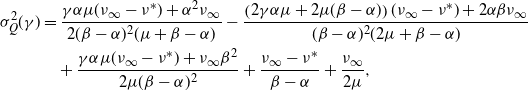 \begin{align}\sigma^2_Q(\gamma)&=\frac{\gamma \alpha \mu (\nu_\infty - \nu^*) + \alpha^2 \nu_\infty }{2(\beta-\alpha)^2(\mu+\beta-\alpha)}-\frac{\left(2\gamma \alpha\mu + 2\mu(\beta-\alpha)\right)(\nu_\infty - \nu^*) + 2\alpha \beta \nu_\infty}{(\beta-\alpha)^2(2\mu+\beta-\alpha)}\nonumber \\&\quad+\frac{\gamma \alpha \mu (\nu_\infty- \nu^*) + \nu_\infty \beta^2 }{2\mu(\beta-\alpha)^2}+\frac{\nu_\infty - \nu^* }{\beta-\alpha}+\frac{\nu_\infty }{2\mu},\end{align}
whereas if $\beta = \alpha$
then
$\beta = \alpha$
then
 \begin{align}\sigma^2_Q(\gamma)=\left(\frac{1}{2\mu} + \frac{\gamma\alpha}{4\mu^2}\right)(\nu_\infty - \nu^*)+\left(\frac{1}{\mu} + \frac{\alpha }{2 \mu^2} + \frac{\alpha^2}{4\mu^3}\right)\nu_\infty,\end{align}
with $\nu_\infty = \frac{(\mu + \beta)\nu^*}{\mu+\beta-\alpha}$
and
$\nu_\infty = \frac{(\mu + \beta)\nu^*}{\mu+\beta-\alpha}$
and $\gamma \in [0,1]$
.
$\gamma \in [0,1]$
.
In Figures 6 and 7 we plot the simulated steady-state distributions of an HESEP with large baseline intensities, as calculated from 100,000 replications. We then also plot the densities corresponding to the upper and lower approximate diffusion distributions as well as an additional candidate approximation with $\gamma = \frac{\mu}{\mu+\beta}$
. We motivate this choice by a ratio of mean approximations of the terms in (37):
$\gamma = \frac{\mu}{\mu+\beta}$
. We motivate this choice by a ratio of mean approximations of the terms in (37):
 \begin{align*}\frac{\frac{(\nu_\infty - \nu^*)^2}{\frac{\nu_\infty}\mu}}{\alpha(\nu_\infty - \nu^*)}=\frac{\mu (\nu_\infty - \nu^*)}{\alpha \nu_\infty}=\frac{\mu}{\mu+\beta}.\end{align*}
In Figure 6 the baseline intensity is equal to 100, whereas in Figure 7 it is 1,000. While there are known limitations of Gaussian approximations for queueing processes, such as those discussed in [Reference Massey and Pender48], we see that these approximations appear to be quite close, particularly for the $\nu^*\,{=}\,1{,}000$
case. The upper and lower bounds predictably over- and under-approximate the tails, while the case of
$\nu^*\,{=}\,1{,}000$
case. The upper and lower bounds predictably over- and under-approximate the tails, while the case of $\gamma = \frac{\mu}{\mu+\beta}$
closely mimics the true distribution.
$\gamma = \frac{\mu}{\mu+\beta}$
closely mimics the true distribution.
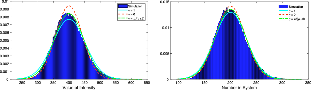
Figure 6. Histogram comparing the simulated steady-state HESEP intensity (left) and queue (right) to their diffusion approximations evaluated at multiple values of $\gamma$
, where
$\gamma$
, where $\nu^* = 100$
,
$\nu^* = 100$
, $\alpha = 3$
,
$\alpha = 3$
, $\beta = 2$
, and
$\beta = 2$
, and $\mu = 2$
.
$\mu = 2$
.
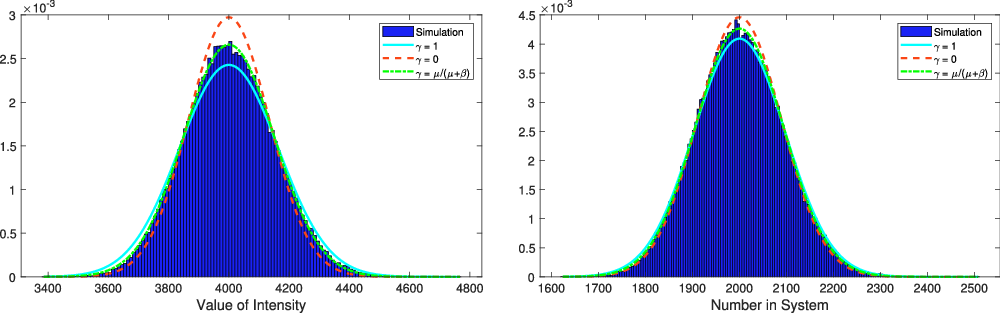
Figure 7. Histogram comparing the simulated steady-state HESEP intensity (left) and queue (right) to their diffusion approximations evaluated at multiple values of $\gamma$
, where
$\gamma$
, where $\nu^* = 1,000$
,
$\nu^* = 1,000$
, $\alpha = 3$
,
$\alpha = 3$
, $\beta = 2$
, and
$\beta = 2$
, and $\mu = 2$
.
$\mu = 2$
.
Appendix C. An ephemeral self-exciting process with finite capacity and blocking
Drawing inspiration from the works that originated queueing theory, we will now consider the change in the ESEP if there is an upper bound on the total number of active exciters. That is, we suppose that there is a finite capacity and no excess buffer beyond them, so that any entities that arrive and find the system full are blocked from entry, thus neither registering an arrival nor causing any excitement. As an employee of the Copenhagen Telephone company, A. K. Erlang developed these pioneering queueing models to determine the probability that a call would be blocked based on the capacity of the telephone network trunk line. Often referred to as the Erlang-B model, this queueing system remains relevant not just to modern telecommunication systems, but broadly across industries as varied as healthcare operations and transportation. (For English translations of the seminal Erlang papers and a biography of the author, see [Reference Brockmeyer, Halstrom and Jensen14].)
In those original works, Erlang supposed that calls arrive perfectly independently, that they have no influence on or relationship with one another. In the remainder of this subsection we investigate the scenario where the calls instead exhibit self-excitement, which is a potential explanation for the over-dispersion that has been seen in industrial call center data, as detailed in e.g. [Reference Ibrahim, Ye, L’Ecuyer and Shen38]. Another potential application for this model is a website that may receive viral traffic but is also liable to crash if there are too many simultaneous visitors. Additionally, the finite-capacity model could be used to represent a restaurant that becomes more enticing the more patrons it has in its limited seating area, as we discussed in the introduction.
To begin, we find the steady-state distribution of this process in Proposition 15. Drawing further inspiration from Erlang’s work, we will refer to this finite-capacity ESEP model as the blocking ephemerally self-exciting process (ESEP-B).
Proposition 15. Let $\eta_t^\textrm{B} = \eta^* + \alpha Q_t^\textrm{B}$
be an ESEP-B, with baseline intensity
$\eta_t^\textrm{B} = \eta^* + \alpha Q_t^\textrm{B}$
be an ESEP-B, with baseline intensity $\eta^* > 0$
, intensity jump
$\eta^* > 0$
, intensity jump $\alpha > 0$
, expiration rate
$\alpha > 0$
, expiration rate $\beta > \alpha$
, and capacity
$\beta > \alpha$
, and capacity $c \in \mathbb{Z}^+$
. That is, if
$c \in \mathbb{Z}^+$
. That is, if $Q_t^\textrm{B} = c$
, any arrivals that occur will be blocked and not recorded. Then the steady-state distribution of the active number in system is given by
$Q_t^\textrm{B} = c$
, any arrivals that occur will be blocked and not recorded. Then the steady-state distribution of the active number in system is given by
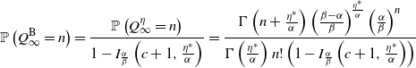 \begin{align}\mathbb{P}\left( Q_\infty^\textrm{B} = n \right)=\frac{ \mathbb{P}\left( Q_\infty^\eta = n \right) }{1 - I_{\frac{\alpha}{\beta}}\left(c+1, \frac{\eta^*}{\alpha}\right)}=\frac{\Gamma\left(n + \frac{\eta^*}{\alpha}\right)\left(\frac{\beta - \alpha}{\beta}\right)^{\!\frac{\eta^*}{\alpha}} \left(\frac{\alpha}{\beta}\right)^{n} }{\Gamma\left(\frac{\eta^*}{\alpha}\right) n!\left(1 - I_{\frac{\alpha}{\beta}}\left(c+1, \frac{\eta^*}{\alpha}\right)\right)}\end{align}
for $0 \leq n \leq c$
and 0 otherwise, where
$0 \leq n \leq c$
and 0 otherwise, where $\mathbb{P}\left( Q_\infty^\eta = n \right)$
is as stated in Theorem 1. Furthermore, the mean and variance of the number in system are given by
$\mathbb{P}\left( Q_\infty^\eta = n \right)$
is as stated in Theorem 1. Furthermore, the mean and variance of the number in system are given by
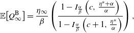 \begin{align}{\mathbb{E}\!\left[Q_\infty^\textrm{B}\right]}&= \frac{\eta_\infty}{\beta}\left(\frac{1 - I_{\frac{\alpha}{\beta}}\left(c, \frac{\eta^*+\alpha}{\alpha}\right)}{1 - I_{\frac{\alpha}{\beta}}\left(c+1, \frac{\eta^*}{\alpha}\right)}\right),\end{align}
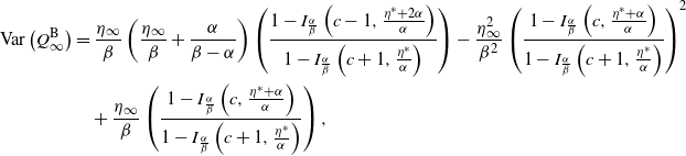 \begin{align}{\textrm{Var}\left({Q_\infty^\textrm{B}}\right)}&= \frac{\eta_\infty}{\beta} \left( \frac{\eta_\infty}{\beta} + \frac{\alpha}{\beta - \alpha} \right) \left( \frac{ 1 - I_{\frac{\alpha}{\beta}}\left(c-1, \frac{\eta^*+ 2\alpha}{\alpha}\right) } {1 - I_{\frac{\alpha}{\beta}}\left(c+1, \frac{\eta^*}{\alpha}\right) } \right)- \frac{\eta_\infty^2}{\beta^2}\left(\frac{1 - I_{\frac{\alpha}{\beta}}\left(c, \frac{\eta^*+\alpha}{\alpha}\right)}{1 - I_{\frac{\alpha}{\beta}}\left(c+1, \frac{\eta^*}{\alpha}\right)}\right)^2\nonumber \\&\quad+ \frac{\eta_\infty}{\beta}\left(\frac{1 - I_{\frac{\alpha}{\beta}}\left(c, \frac{\eta^*+\alpha}{\alpha}\right)}{1 - I_{\frac{\alpha}{\beta}}\left(c+1, \frac{\eta^*}{\alpha}\right)}\right),\end{align}
where $\eta_\infty = \frac{\beta \eta^*}{\beta - \alpha}$
and
$\eta_\infty = \frac{\beta \eta^*}{\beta - \alpha}$
and
 \begin{align*}I_z(a,b) = \frac{\Gamma (a+b)}{\Gamma (a) \Gamma (b)} \int_0^z x^{a-1}(1-x)^{b-1} \textrm{d}x\end{align*}
for $z \in [0,1]$
,
$z \in [0,1]$
, $a > 0$
, and
$a > 0$
, and $b > 0$
is the regularized incomplete beta function.
$b > 0$
is the regularized incomplete beta function.
Proof. To prove each of these statements, we first note that for $k \in \mathbb{Z}^+$
,
$k \in \mathbb{Z}^+$
, $x > 0$
, and
$x > 0$
, and $p \in (0,1)$
,
$p \in (0,1)$
,
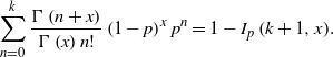 \begin{align}\sum_{n=0}^k\frac{\Gamma\left(n + x\right)}{\Gamma\left(x\right) n! }\left(1 - p\right)^{x}p^n=1 - I_{p}\left(k+1, x\right)\!.\end{align}
Hence, we can use (47) to see that
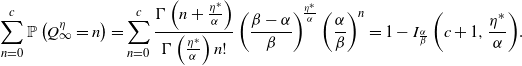 \begin{align*}\sum_{n=0}^c\mathbb{P}\left( Q_\infty^\eta = n \right)=\sum_{n=0}^c\frac{\Gamma\left(n + \frac{\eta^*}{\alpha}\right)}{\Gamma\left(\frac{\eta^*}{\alpha}\right) n! }\left(\frac{\beta - \alpha}{\beta}\right)^{\!\frac{\eta^*}{\alpha}}\left(\frac{\alpha}{\beta}\right)^n=1 - I_{\frac{\alpha}{\beta}}\left(c+1, \frac{\eta^*}{\alpha}\right)\!.\end{align*}
Because the ESEP is a birth–death process, it is reversible. Thus, by truncation we achieve the steady-state distribution; see e.g. Corollary 1.10 in [Reference Kelly40]. Then the steady-state mean of the number in system is given by
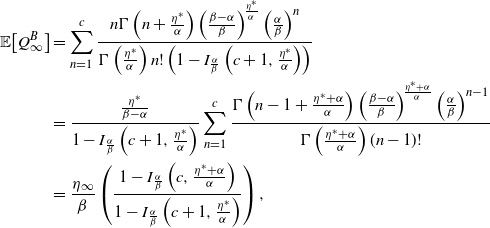 \begin{align*}{\mathbb{E}\!\left[Q_\infty^B\right]}&=\sum_{n=1}^c\frac{n\Gamma\left(n + \frac{\eta^*}{\alpha}\right)\left(\frac{\beta - \alpha}{\beta}\right)^{\!\frac{\eta^*}{\alpha}} \left(\frac{\alpha}{\beta}\right)^{n} }{\Gamma\left(\frac{\eta^*}{\alpha}\right) n!\left(1 - I_{\frac{\alpha}{\beta}}\left(c+1, \frac{\eta^*}{\alpha}\right)\right)} \\ & = \frac{ \frac{\eta^*}{\beta-\alpha} } {1 - I_{\frac{\alpha}{\beta}}\left(c+1, \frac{\eta^*}{\alpha}\right) }\sum_{n=1}^c\frac{\Gamma\left(n - 1 + \frac{\eta^* + \alpha}{\alpha}\right)\left(\frac{\beta - \alpha}{\beta}\right)^{\!\frac{\eta^* + \alpha}{\alpha}} \left(\frac{\alpha}{\beta}\right)^{n-1} }{\Gamma\left(\frac{\eta^*+\alpha}{\alpha}\right) (n-1)!} \\ & = \frac{\eta_\infty}{\beta}\left(\frac{1 - I_{\frac{\alpha}{\beta}}\left(c, \frac{\eta^*+\alpha}{\alpha}\right)}{1 - I_{\frac{\alpha}{\beta}}\left(c+1, \frac{\eta^*}{\alpha}\right)}\right),\end{align*}
where we have again used (47) to simplify the summation. Likewise, the second moment in steady state can be written as
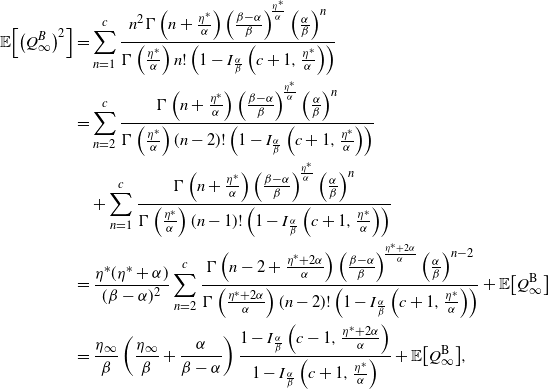 \begin{align*}{\mathbb{E}\!\left[\left(Q_\infty^B\right)^2\right]}&=\sum_{n=1}^c\frac{n^2\Gamma\left(n + \frac{\eta^*}{\alpha}\right)\left(\frac{\beta - \alpha}{\beta}\right)^{\!\frac{\eta^*}{\alpha}} \left(\frac{\alpha}{\beta}\right)^{n} }{\Gamma\left(\frac{\eta^*}{\alpha}\right) n!\left(1 - I_{\frac{\alpha}{\beta}}\left(c+1, \frac{\eta^*}{\alpha}\right)\right)} \\ & = \sum_{n=2}^c \frac{\Gamma\left(n + \frac{\eta^*}{\alpha}\right)\left(\frac{\beta - \alpha}{\beta}\right)^{\!\frac{\eta^*}{\alpha}} \left(\frac{\alpha}{\beta}\right)^{n} }{\Gamma\left(\frac{\eta^*}{\alpha}\right) (n-2)!\left(1 - I_{\frac{\alpha}{\beta}}\left(c+1, \frac{\eta^*}{\alpha}\right)\right)} \\ & \quad + \sum_{n=1}^c \frac{\Gamma\left(n + \frac{\eta^*}{\alpha}\right)\left(\frac{\beta - \alpha}{\beta}\right)^{\!\frac{\eta^*}{\alpha}} \left(\frac{\alpha}{\beta}\right)^{n} }{\Gamma\left(\frac{\eta^*}{\alpha}\right) (n-1)!\left(1 - I_{\frac{\alpha}{\beta}}\left(c+1, \frac{\eta^*}{\alpha}\right)\right)} \\ & = \frac{\eta^*(\eta^* + \alpha)}{(\beta-\alpha)^2}\sum_{n=2}^c\frac{\Gamma\left(n - 2 + \frac{\eta^*+ 2\alpha}{\alpha}\right)\left(\frac{\beta - \alpha}{\beta}\right)^{\!\frac{\eta^* + 2\alpha}{\alpha}} \left(\frac{\alpha}{\beta}\right)^{n-2} }{\Gamma\left(\frac{\eta^* + 2 \alpha}{\alpha}\right) (n-2)!\left(1 - I_{\frac{\alpha}{\beta}}\left(c+1, \frac{\eta^*}{\alpha}\right)\right)} + {\mathbb{E}\!\left[Q_\infty^\textrm{B}\right]} \\ & = \frac{\eta_\infty}{\beta} \left( \frac{\eta_\infty}{\beta} + \frac{\alpha}{\beta - \alpha} \right) \frac{ 1 - I_{\frac{\alpha}{\beta}}\left(c-1, \frac{\eta^*+2\alpha}{\alpha}\right) }{ 1 - I_{\frac{\alpha}{\beta}}\left(c+1, \frac{\eta^*}{\alpha}\right) } + {\mathbb{E}\!\left[Q_\infty^\textrm{B}\right]},\end{align*}
where once more these sums have been simplified through (47).
As an illustration of these findings, we now plot both the steady-state distribution and the mean and variance of this blocking system in Figure 8. As can be observed in the figure, the system remains over-dispersed even when truncated. We can observe further that this holds in generality as follows. For this, we state two known properties of the regularized incomplete beta function:
 \begin{align}I_z(a,b) = I_z(a+1,b) + \frac{z^a(1-z)^b}{a B(a,b)}, & & I_z(a,b+1) = I_z(a,b) + \frac{z^a(1-z)^b}{b B(a,b)} ,\end{align}
where $B(a,b) = \frac{\Gamma (a+b)}{\Gamma(a)\Gamma(b)}$
is the beta function. Using these together, we can observe that
$B(a,b) = \frac{\Gamma (a+b)}{\Gamma(a)\Gamma(b)}$
is the beta function. Using these together, we can observe that
 \begin{align*}I_z(a,b) > I_z(a+1,b-1).\end{align*}
Thus, we can see that
 \begin{align*}I_{\frac{\alpha}{\beta}}\left(c+1, \frac{\eta^*}{\alpha}\right) < I_{\frac{\alpha}{\beta}}\left(c, \frac{\eta^* + \alpha}{\alpha}\right) < I_{\frac{\alpha}{\beta}}\left(c-1, \frac{\eta^*+2\alpha}{\alpha}\right) < 1,\end{align*}
which implies
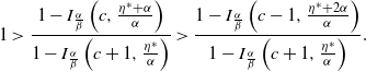 \begin{align*}1>\frac{1 - I_{\frac{\alpha}{\beta}}\left(c, \frac{\eta^*+\alpha}{\alpha}\right)}{1 - I_{\frac{\alpha}{\beta}}\left(c+1, \frac{\eta^*}{\alpha}\right)}>\frac{1 - I_{\frac{\alpha}{\beta}}\left(c-1, \frac{\eta^*+2\alpha}{\alpha}\right)}{1 - I_{\frac{\alpha}{\beta}}\left(c+1, \frac{\eta^*}{\alpha}\right)}.\end{align*}
We now note that the variance is written as the sum of the mean and a positive term and is thus over-dispersed.
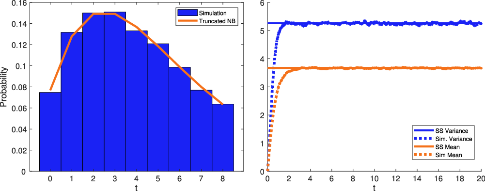
Figure 8. Steady-state distribution (left) and mean and variance (right) of the ESEP-B with $\eta^* = 5$
,
$\eta^* = 5$
, $\alpha = 2$
,
$\alpha = 2$
, $\beta = 3$
, and
$\beta = 3$
, and $c = 8$
, based on 10,000 replications.
$c = 8$
, based on 10,000 replications.
We can also note that in the classical Erlang-B model, the famous ‘Poisson arrivals see time averages’ (PASTA) result implies that the steady-state fraction of arrivals that are blocked is equal to the probability that the queue is at capacity in steady-state; see [Reference Wolff61]. This is not so for the ESEP-B, as the arrival rate is state-dependent and, more specifically, increases with the queue length. However, in Proposition 16 we find that an equivalent result holds asymptotically as the baseline intensity and the capacity grow large simultaneously. We note that large baseline intensity and capacity are realistic scenarios for many practically relevant applications, including the aforementioned website-crashing scenario.
Proposition 16. Let $\eta_t^\textrm{B} = \eta^* + \alpha Q_t^\textrm{B}$
be an ESEP-B, with baseline intensity
$\eta_t^\textrm{B} = \eta^* + \alpha Q_t^\textrm{B}$
be an ESEP-B, with baseline intensity $\eta^* > 0$
, intensity jump
$\eta^* > 0$
, intensity jump $\alpha > 0$
, exponential service rate
$\alpha > 0$
, exponential service rate $\beta > \alpha$
, and capacity
$\beta > \alpha$
, and capacity $c \in \mathbb{Z}^+$
. Then the fraction of arrivals in steady-state that are blocked,
$c \in \mathbb{Z}^+$
. Then the fraction of arrivals in steady-state that are blocked, $\pi_{\textrm{B}}$
, is given by
$\pi_{\textrm{B}}$
, is given by
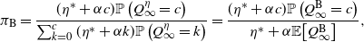 \begin{align}\pi_{\textrm{B}}&=\frac{(\eta^* + \alpha c)\mathbb{P}\left( Q_\infty^\eta = c \right)}{\sum_{k=0}^c (\eta^* + \alpha k) \mathbb{P}\left( Q_\infty^\eta = k \right)}=\frac{(\eta^* + \alpha c) \mathbb{P}\left( Q_\infty^\textrm{B} = c \right)}{\eta^* + \alpha {\mathbb{E}\!\left[Q_\infty^\textrm{B}\right]}},\end{align}
where $\mathbb{P}\left( Q_\infty^\eta = k \right)$
is as given in Theorem 1 and
$\mathbb{P}\left( Q_\infty^\eta = k \right)$
is as given in Theorem 1 and $\mathbb{P}\left( Q_\infty^\textrm{B} = c \right)$
and
$\mathbb{P}\left( Q_\infty^\textrm{B} = c \right)$
and ${\mathbb{E}\!\left[Q_\infty^\textrm{B}\right]}$
are as given in Proposition 15. Moreover, if the baseline intensity and the capacity are redefined to be
${\mathbb{E}\!\left[Q_\infty^\textrm{B}\right]}$
are as given in Proposition 15. Moreover, if the baseline intensity and the capacity are redefined to be $\eta^* n$
and c n for
$\eta^* n$
and c n for $n \in \mathbb{Z}^+$
, then
$n \in \mathbb{Z}^+$
, then
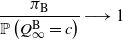 \begin{align}\frac{\pi_{\textrm{B}}}{\mathbb{P}\left( Q_\infty^\textrm{B} = c \right)}&\longrightarrow 1\end{align}
as $n \to \infty$
.
$n \to \infty$
.
Proof. The expression for the steady-state fraction of arrivals blocked, $\pi_\textrm{B}$
, in (49) follows as a direct consequence from observing that
$\pi_\textrm{B}$
, in (49) follows as a direct consequence from observing that $\eta^* + \alpha k$
is the arrival rate when the queue is in state k. We are thus left to prove (50). By use of (49), we have that the ratio of
$\eta^* + \alpha k$
is the arrival rate when the queue is in state k. We are thus left to prove (50). By use of (49), we have that the ratio of $\pi_{B}$
and
$\pi_{B}$
and $\mathbb{P}\left( Q_\infty^\textrm{B} = c \right)$
is
$\mathbb{P}\left( Q_\infty^\textrm{B} = c \right)$
is
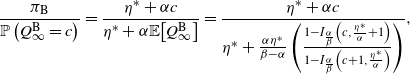 \begin{align*}\frac{\pi_\textrm{B}}{\mathbb{P}\left( Q_\infty^\textrm{B} = c \right)}&=\frac{\eta^* + \alpha c }{\eta^* + \alpha {\mathbb{E}\!\left[Q_\infty^\textrm{B}\right]}}=\frac{\eta^* + \alpha c }{\eta^* + \frac{\alpha \eta^*}{\beta - \alpha}\left(\frac{1 - I_{\frac{\alpha}{\beta}}\left(c, \frac{\eta^*}{\alpha}+1\right)}{1 - I_{\frac{\alpha}{\beta}}\left(c+1, \frac{\eta^*}{\alpha}\right)}\right)},\end{align*}
by Proposition 15. Substituting in the scaled forms of the baseline intensity and capacity, $\eta^* n$
and cn, and then dividing the numerator and denominator by cn, this is
$\eta^* n$
and cn, and then dividing the numerator and denominator by cn, this is
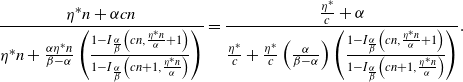 \begin{align*}\frac{\eta^*n + \alpha cn }{\eta^*n + \frac{\alpha \eta^*n}{\beta - \alpha}\left(\frac{1 - I_{\frac{\alpha}{\beta}}\left(cn, \frac{\eta^*n}{\alpha}+1\right)}{1 - I_{\frac{\alpha}{\beta}}\left(cn+1, \frac{\eta^*n}{\alpha}\right)}\right)}&=\frac{\frac{\eta^*}{c} + \alpha }{\frac{\eta^*}{c} + \frac{\eta^*}{c}\left(\frac{\alpha }{\beta - \alpha}\right)\left(\frac{1 - I_{\frac{\alpha}{\beta}}\left(cn, \frac{\eta^*n}{\alpha}+1\right)}{1 - I_{\frac{\alpha}{\beta}}\left(cn+1, \frac{\eta^*n}{\alpha}\right)}\right)}.\end{align*}
From the definition and symmetry of the regularized incomplete beta function, we can note that the ratio of these functions is such that
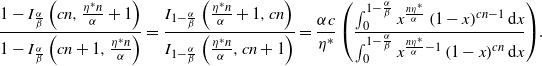 \begin{align*}\frac{1 - I_{\frac{\alpha}{\beta}}\left(cn, \frac{\eta^*n}{\alpha}+1\right)}{1 - I_{\frac{\alpha}{\beta}}\left(cn+1, \frac{\eta^*n}{\alpha}\right)}&=\frac{I_{1-\frac{\alpha}{\beta}}\left(\frac{\eta^*n}{\alpha}+1, cn\right)}{I_{1-\frac{\alpha}{\beta}}\left(\frac{\eta^*n}{\alpha}, cn + 1\right)}=\frac{\alpha c}{\eta^*}\left(\frac{ \int_0^{1-\frac{\alpha}{\beta}} x^{\frac{n\eta^*}{\alpha}}\left(1-x\right)^{cn-1}\textrm{d}x}{ \int_0^{1-\frac{\alpha}{\beta}} x^{\frac{n\eta^*}{\alpha}-1}\left(1-x\right)^{cn}\textrm{d}x}\right)\!.\end{align*}
Now, recognizing an identity for the hypergeometric function $\,_2F_1(a,b;\, c;\, z)$
, we can re-express this ratio as
$\,_2F_1(a,b;\, c;\, z)$
, we can re-express this ratio as
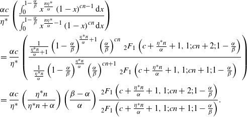 \begin{align*}&\frac{\alpha c}{\eta^*}\left(\frac{ \int_0^{1-\frac{\alpha}{\beta}} x^{\frac{n\eta^*}{\alpha}}\left(1-x\right)^{cn-1}\textrm{d}x}{ \int_0^{1-\frac{\alpha}{\beta}} x^{\frac{n\eta^*}{\alpha}-1}\left(1-x\right)^{cn}\textrm{d}x}\right)\\&=\frac{\alpha c}{\eta^*}\left(\frac{\frac{1}{\frac{\eta^* n}{\alpha} + 1} \left(1-\frac{\alpha}{\beta}\right)^{\!\frac{\eta^* n}{\alpha}+1}\left(\frac{\alpha}{\beta}\right)^{c n} \,_2F_1 \left(c+\frac{\eta^* n}{\alpha}+1,1;cn+2;1-\frac{\alpha}{\beta}\right)}{\frac{1}{\frac{\eta^* n}{\alpha}} \left(1-\frac{\alpha}{\beta}\right)^{\!\frac{\eta^* n}{\alpha}}\left(\frac{\alpha}{\beta}\right)^{c n + 1} \,_2F_1 \left(c+\frac{\eta^* n}{\alpha}+1,1;cn+1;1-\frac{\alpha}{\beta}\right)}\right)\\&=\frac{\alpha c}{\eta^*}\left(\frac{\eta^* n}{\eta^* n + \alpha}\right)\left(\frac{\beta - \alpha}{\alpha}\right)\frac{\,_2F_1 \left(c+\frac{\eta^* n}{\alpha}+1,1;cn+2;1-\frac{\alpha}{\beta}\right)}{ \,_2F_1 \left(c+\frac{\eta^* n}{\alpha}+1,1;cn+1;1-\frac{\alpha}{\beta}\right)}.\end{align*}
As $n \to \infty$
, this yields
$n \to \infty$
, this yields
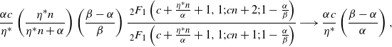 \begin{align*}\frac{\alpha c}{\eta^*}\left(\frac{\eta^* n}{\eta^* n + \alpha}\right)\left(\frac{\beta - \alpha}{\beta}\right)\frac{\,_2F_1 \left(c+\frac{\eta^* n}{\alpha}+1,1;cn+2;1-\frac{\alpha}{\beta}\right)}{ \,_2F_1 \left(c+\frac{\eta^* n}{\alpha}+1,1;cn+1;1-\frac{\alpha}{\beta}\right)}\longrightarrow \frac{\alpha c}{\eta^*}\left(\frac{\beta - \alpha}{\alpha}\right),\end{align*}
which implies that
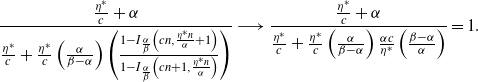 \begin{align*}\frac{\frac{\eta^*}{c} + \alpha }{\frac{\eta^*}{c} + \frac{\eta^*}{c}\left(\frac{\alpha }{\beta - \alpha}\right)\left(\frac{1 - I_{\frac{\alpha}{\beta}}\left(cn, \frac{\eta^*n}{\alpha}+1\right)}{1 - I_{\frac{\alpha}{\beta}}\left(cn+1, \frac{\eta^*n}{\alpha}\right)}\right)}\longrightarrow \frac{\frac{\eta^*}{c} + \alpha }{\frac{\eta^*}{c} + \frac{\eta^*}{c}\left(\frac{\alpha }{\beta - \alpha}\right)\frac{\alpha c}{\eta^*}\left(\frac{\beta - \alpha}{\alpha}\right)}=1.\end{align*}
This completes the proof.
As an example of the convergence stated in Proposition 16, we compare the probability of the system being at capacity and the fraction of blocked arrivals below in Figure 9. In this figure, $\eta^*$
and c are increased simultaneously according to a fixed ratio. Although at the initial values it is clear that a PASTA-esque result does not hold, as the baseline intensity and capacity both increase one can see that the two curves tend toward one another in each of the different parameter settings.
$\eta^*$
and c are increased simultaneously according to a fixed ratio. Although at the initial values it is clear that a PASTA-esque result does not hold, as the baseline intensity and capacity both increase one can see that the two curves tend toward one another in each of the different parameter settings.
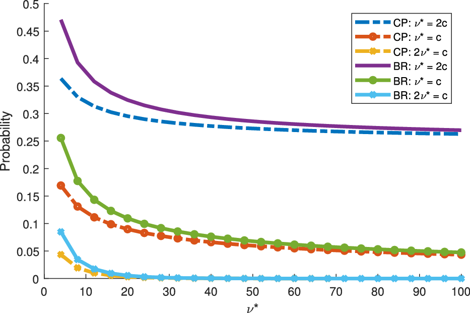
Figure 9. Comparison of the ratio of blocked arrivals (BR) and the probability of system being at capacity (CP) when $\eta^*$
and c are increased simultaneously, for
$\eta^*$
and c are increased simultaneously, for $\alpha = 2$
and
$\alpha = 2$
and $\beta = 3$
.
$\beta = 3$
.
Appendix D. Proof of Proposition 3
Proof. Using Proposition 11, we proceed through use of exponential identities for the hyperbolic functions. Specifically, we will make use of the following:
 \begin{align}\tanh(x)&=\frac{e^x - e^{-x}}{e^x + e^{-x}},\end{align}
 \begin{align}\cosh(x)&=\frac{e^x + e^{-x}}2,\end{align}
and
 \begin{align}\tanh^{-1}(x)&=\frac{1}{2}\log\left(\frac{1 + x}{1-x}\right)\!.\end{align}
Using these identities we can further observe that
 \begin{align*}\cosh\left(\tanh^{-1}(x)\right)&=\frac{e^{\tanh^{-1}(x)} + e^{-\tanh^{-1}(x)}}2=\frac{\left(\frac{1 + x}{1-x}\right)^{\!\frac{1}{2}}+\left(\frac{1 - x}{1 + x}\right)^{\!\frac{1}{2}}}2.\end{align*}
Now, for any time $t \geq 0$
we can note that
$t \geq 0$
we can note that $N_t = Q_t + D_t$
. Thus, we have that
$N_t = Q_t + D_t$
. Thus, we have that
 \begin{align*}{\mathbb{E}\!\left[z^{N_{t}}\right]} = {\mathbb{E}\!\left[z^{Q_t}z^{D_t}\right]} = G(z,z,t),\end{align*}
where $G(z_1,z_2,t)$
is as given in Proposition 11. Setting
$G(z_1,z_2,t)$
is as given in Proposition 11. Setting $z_1 = z_2 = z$
and
$z_1 = z_2 = z$
and $D_0 = N_0 - Q_0$
, this is
$D_0 = N_0 - Q_0$
, this is
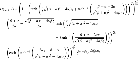 \begin{align}&G(z, z, t)=\left(1-\left(\tanh\left(\frac{t}2 \sqrt{(\beta+\alpha)^2 - 4\alpha\beta z}+\tanh^{-1}\left(\frac{\beta+\alpha-2\alpha z }{\sqrt{(\beta+\alpha)^2 - 4\alpha\beta z}} \right)\right)\right)^2\right)^{\!\frac{\eta^*}{2\alpha}}\nonumber \\&\quad\cdot \left(\frac{\beta + \alpha}{2\alpha}-\frac{\sqrt{(\beta+\alpha)^2 - 4\alpha\beta z}}{2\alpha}\tanh \left(\frac{t}2 \sqrt{(\beta+\alpha)^2 - 4\alpha\beta z} \right.\right.\nonumber\\&\quad\quad\quad\qquad\quad\quad\quad\quad\quad\quad\quad\quad\quad + \left.\left. \tanh^{-1}\left(\frac{ \beta+\alpha-2\alpha z}{\sqrt{(\beta+\alpha)^2 - 4\alpha\beta z}} \right) \right)\right)^{Q_0}\nonumber \\&\quad\cdot \left(\cosh \left(\tanh^{-1}\left(\frac{2\alpha z - \beta - \alpha}{\sqrt{(\beta+\alpha)^2 - 4\alpha\beta z}} \right)\right)\right)^{\!\frac{\eta^*}{\alpha}}z^{N_0 - Q_0} e^{\frac{\eta^*(\beta-\alpha)}{2\alpha}t}.\end{align}
Using the hyperbolic identities and simplifying, this is
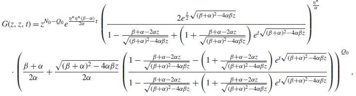 \begin{align*}&G(z, z, t)=z^{N_0 - Q_0} e^{\frac{\eta^*\eta^*(\beta-\alpha)}{2\alpha}t}\left(\frac{2e^{\frac{t}{2} \sqrt{(\beta+\alpha)^2 - 4\alpha\beta z}}}{1-\frac{ \beta+\alpha-2\alpha z}{\sqrt{(\beta+\alpha)^2 - 4\alpha\beta z}}+\left(1 + \frac{ \beta+\alpha-2\alpha z}{\sqrt{(\beta+\alpha)^2 - 4\alpha\beta z}}\right)e^{t \sqrt{(\beta+\alpha)^2 - 4\alpha\beta z}}}\right)^{\!\frac{\eta^*}{\alpha}}\nonumber \\&\quad\cdot \left(\frac{\beta + \alpha}{2\alpha}+\frac{\sqrt{(\beta+\alpha)^2 - 4\alpha\beta z}}{2\alpha}\left(\frac{1-\frac{ \beta+\alpha-2\alpha z}{\sqrt{(\beta+\alpha)^2 - 4\alpha\beta z}}-\left(1 + \frac{ \beta+\alpha-2\alpha z}{\sqrt{(\beta+\alpha)^2 - 4\alpha\beta z}}\right)e^{t \sqrt{(\beta+\alpha)^2 - 4\alpha\beta z}}}{1-\frac{ \beta+\alpha-2\alpha z}{\sqrt{(\beta+\alpha)^2 - 4\alpha\beta z}}+\left(1 + \frac{ \beta+\alpha-2\alpha z}{\sqrt{(\beta+\alpha)^2 - 4\alpha\beta z}}\right)e^{t \sqrt{(\beta+\alpha)^2 - 4\alpha\beta z}}}\right)\right)^{Q_0},\end{align*}
which is the stated result. However, the simplifications used to reach this form require several steps, which we present individually now. We start with the hyperbolic tangent function that appears on the first and second lines of (54). Using (51) and (53), this is
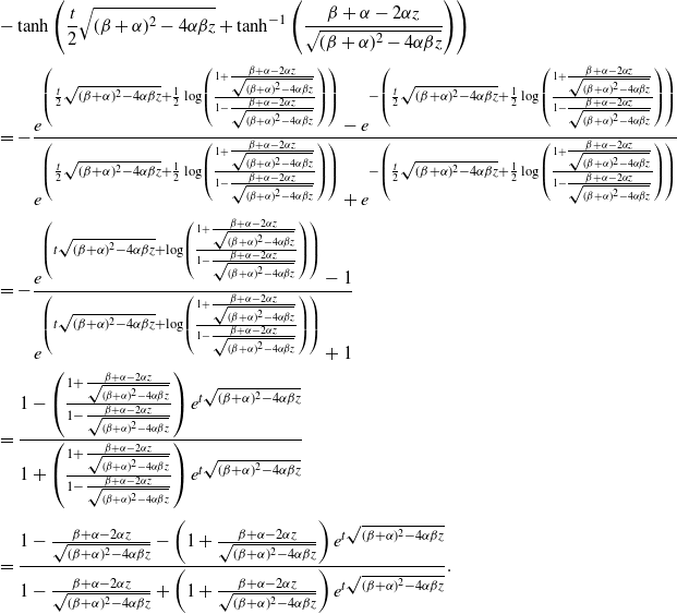 \begin{align*}&-\tanh \left(\frac{t}2 \sqrt{(\beta+\alpha)^2 - 4\alpha\beta z} + \tanh^{-1}\left(\frac{ \beta+\alpha-2\alpha z}{\sqrt{(\beta+\alpha)^2 - 4\alpha\beta z}} \right) \right)\\[3pt]&=-\frac{e^{\left(\frac{t}2 \sqrt{(\beta+\alpha)^2 - 4\alpha\beta z}+\frac{1}{2}\log\left(\frac{1 + \frac{ \beta+\alpha-2\alpha z}{\sqrt{(\beta+\alpha)^2 - 4\alpha\beta z}}}{1-\frac{ \beta+\alpha-2\alpha z}{\sqrt{(\beta+\alpha)^2 - 4\alpha\beta z}}}\right)\right)}-e^{-\left(\frac{t}2 \sqrt{(\beta+\alpha)^2 - 4\alpha\beta z}+\frac{1}{2}\log\left(\frac{1 + \frac{ \beta+\alpha-2\alpha z}{\sqrt{(\beta+\alpha)^2 - 4\alpha\beta z}}}{1-\frac{ \beta+\alpha-2\alpha z}{\sqrt{(\beta+\alpha)^2 - 4\alpha\beta z}}}\right)\right)}}{e^{\left(\frac{t}2 \sqrt{(\beta+\alpha)^2 - 4\alpha\beta z}+\frac{1}{2}\log\left(\frac{1 + \frac{ \beta+\alpha-2\alpha z}{\sqrt{(\beta+\alpha)^2 - 4\alpha\beta z}}}{1-\frac{ \beta+\alpha-2\alpha z}{\sqrt{(\beta+\alpha)^2 - 4\alpha\beta z}}}\right)\right)}+e^{-\left(\frac{t}2 \sqrt{(\beta+\alpha)^2 - 4\alpha\beta z}+\frac{1}{2}\log\left(\frac{1 + \frac{ \beta+\alpha-2\alpha z}{\sqrt{(\beta+\alpha)^2 - 4\alpha\beta z}}}{1-\frac{ \beta+\alpha-2\alpha z}{\sqrt{(\beta+\alpha)^2 - 4\alpha\beta z}}}\right)\right)}}\\[3pt]&=-\frac{e^{\left(t \sqrt{(\beta+\alpha)^2 - 4\alpha\beta z}+\log\left(\frac{1 + \frac{ \beta+\alpha-2\alpha z}{\sqrt{(\beta+\alpha)^2 - 4\alpha\beta z}}}{1-\frac{ \beta+\alpha-2\alpha z}{\sqrt{(\beta+\alpha)^2 - 4\alpha\beta z}}}\right)\right)}-1}{e^{\left(t \sqrt{(\beta+\alpha)^2 - 4\alpha\beta z}+\log\left(\frac{1 + \frac{ \beta+\alpha-2\alpha z}{\sqrt{(\beta+\alpha)^2 - 4\alpha\beta z}}}{1-\frac{ \beta+\alpha-2\alpha z}{\sqrt{(\beta+\alpha)^2 - 4\alpha\beta z}}}\right)\right)}+1}\\[3pt]&=\frac{1-\left(\frac{1 + \frac{ \beta+\alpha-2\alpha z}{\sqrt{(\beta+\alpha)^2 - 4\alpha\beta z}}}{1-\frac{ \beta+\alpha-2\alpha z}{\sqrt{(\beta+\alpha)^2 - 4\alpha\beta z}}}\right)e^{t \sqrt{(\beta+\alpha)^2 - 4\alpha\beta z}}}{1+\left(\frac{1 + \frac{ \beta+\alpha-2\alpha z}{\sqrt{(\beta+\alpha)^2 - 4\alpha\beta z}}}{1-\frac{ \beta+\alpha-2\alpha z}{\sqrt{(\beta+\alpha)^2 - 4\alpha\beta z}}}\right)e^{t \sqrt{(\beta+\alpha)^2 - 4\alpha\beta z}}}\\[3pt]&=\frac{1-\frac{ \beta+\alpha-2\alpha z}{\sqrt{(\beta+\alpha)^2 - 4\alpha\beta z}}-\left(1 + \frac{ \beta+\alpha-2\alpha z}{\sqrt{(\beta+\alpha)^2 - 4\alpha\beta z}}\right)e^{t \sqrt{(\beta+\alpha)^2 - 4\alpha\beta z}}}{1-\frac{ \beta+\alpha-2\alpha z}{\sqrt{(\beta+\alpha)^2 - 4\alpha\beta z}}+\left(1 + \frac{ \beta+\alpha-2\alpha z}{\sqrt{(\beta+\alpha)^2 - 4\alpha\beta z}}\right)e^{t \sqrt{(\beta+\alpha)^2 - 4\alpha\beta z}}}.\end{align*}
Thus, the second line of (54) can be simplified to
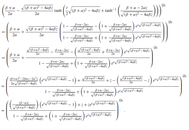 \begin{align*}&\left(\frac{\beta + \alpha}{2\alpha}-\frac{\sqrt{(\beta+\alpha)^2 - 4\alpha\beta z}}{2\alpha}\tanh \left(\frac{t}2 \sqrt{(\beta+\alpha)^2 - 4\alpha\beta z} + \tanh^{-1}\left(\frac{ \beta+\alpha-2\alpha z}{\sqrt{(\beta+\alpha)^2 - 4\alpha\beta z}} \right) \right)\right)^{Q_0}\\[3pt]&=\left(\frac{\beta + \alpha}{2\alpha}+\frac{\sqrt{(\beta+\alpha)^2 - 4\alpha\beta z}}{2\alpha}\left(\frac{1-\frac{ \beta+\alpha-2\alpha z}{\sqrt{(\beta+\alpha)^2 - 4\alpha\beta z}}-\left(1 + \frac{ \beta+\alpha-2\alpha z}{\sqrt{(\beta+\alpha)^2 - 4\alpha\beta z}}\right)e^{t \sqrt{(\beta+\alpha)^2 - 4\alpha\beta z}}}{1-\frac{ \beta+\alpha-2\alpha z}{\sqrt{(\beta+\alpha)^2 - 4\alpha\beta z}}+\left(1 + \frac{ \beta+\alpha-2\alpha z}{\sqrt{(\beta+\alpha)^2 - 4\alpha\beta z}}\right)e^{t \sqrt{(\beta+\alpha)^2 - 4\alpha\beta z}}}\right)\right)^{Q_0}\\[3pt]&=\left(\frac{\beta + \alpha}{2\alpha}+\frac{\frac{\sqrt{(\beta+\alpha)^2 - 4\alpha\beta z}}{2\alpha} - \frac{ \beta+\alpha-2\alpha z}{2\alpha}-\left(\frac{\sqrt{(\beta+\alpha)^2 - 4\alpha\beta z}}{2\alpha} + \frac{ \beta+\alpha-2\alpha z}{2\alpha}\right)e^{t \sqrt{(\beta+\alpha)^2 - 4\alpha\beta z}}}{1-\frac{ \beta+\alpha-2\alpha z}{\sqrt{(\beta+\alpha)^2 - 4\alpha\beta z}}+\left(1 + \frac{ \beta+\alpha-2\alpha z}{\sqrt{(\beta+\alpha)^2 - 4\alpha\beta z}}\right)e^{t \sqrt{(\beta+\alpha)^2 - 4\alpha\beta z}}}\right)^{Q_0}\\
&=\left(\frac{\frac{ (\beta+\alpha)^2-2\beta\alpha z-2\alpha^2z}{2\alpha\sqrt{(\beta+\alpha)^2 - 4\alpha\beta z}}\left(e^{t \sqrt{(\beta+\alpha)^2 - 4\alpha\beta z}}-1\right)+\frac{\sqrt{(\beta+\alpha)^2 - 4\alpha\beta z}}{2\alpha} + z-\left(\frac{\sqrt{(\beta+\alpha)^2 - 4\alpha\beta z}}{2\alpha} - z\right)e^{t \sqrt{(\beta+\alpha)^2 - 4\alpha\beta z}}}{1-\frac{ \beta+\alpha-2\alpha z}{\sqrt{(\beta+\alpha)^2 - 4\alpha\beta z}}+\left(1 + \frac{ \beta+\alpha-2\alpha z}{\sqrt{(\beta+\alpha)^2 - 4\alpha\beta z}}\right)e^{t \sqrt{(\beta+\alpha)^2 - 4\alpha\beta z}}}\right)^{Q_0}\\&=\left(\frac{\left(\frac{ (\beta -\alpha) z}{\sqrt{(\beta+\alpha)^2 - 4\alpha\beta z}}\right)\left(e^{t \sqrt{(\beta+\alpha)^2 - 4\alpha\beta z}}-1\right)+ z+ze^{t \sqrt{(\beta+\alpha)^2 - 4\alpha\beta z}}}{1-\frac{ \beta+\alpha-2\alpha z}{\sqrt{(\beta+\alpha)^2 - 4\alpha\beta z}}+\left(1 + \frac{ \beta+\alpha-2\alpha z}{\sqrt{(\beta+\alpha)^2 - 4\alpha\beta z}}\right)e^{t \sqrt{(\beta+\alpha)^2 - 4\alpha\beta z}}}\right)^{Q_0}.
\end{align*}
\begin{align*}&\left(\frac{\beta + \alpha}{2\alpha}-\frac{\sqrt{(\beta+\alpha)^2 - 4\alpha\beta z}}{2\alpha}\tanh \left(\frac{t}2 \sqrt{(\beta+\alpha)^2 - 4\alpha\beta z} + \tanh^{-1}\left(\frac{ \beta+\alpha-2\alpha z}{\sqrt{(\beta+\alpha)^2 - 4\alpha\beta z}} \right) \right)\right)^{Q_0}\\[3pt]&=\left(\frac{\beta + \alpha}{2\alpha}+\frac{\sqrt{(\beta+\alpha)^2 - 4\alpha\beta z}}{2\alpha}\left(\frac{1-\frac{ \beta+\alpha-2\alpha z}{\sqrt{(\beta+\alpha)^2 - 4\alpha\beta z}}-\left(1 + \frac{ \beta+\alpha-2\alpha z}{\sqrt{(\beta+\alpha)^2 - 4\alpha\beta z}}\right)e^{t \sqrt{(\beta+\alpha)^2 - 4\alpha\beta z}}}{1-\frac{ \beta+\alpha-2\alpha z}{\sqrt{(\beta+\alpha)^2 - 4\alpha\beta z}}+\left(1 + \frac{ \beta+\alpha-2\alpha z}{\sqrt{(\beta+\alpha)^2 - 4\alpha\beta z}}\right)e^{t \sqrt{(\beta+\alpha)^2 - 4\alpha\beta z}}}\right)\right)^{Q_0}\\[3pt]&=\left(\frac{\beta + \alpha}{2\alpha}+\frac{\frac{\sqrt{(\beta+\alpha)^2 - 4\alpha\beta z}}{2\alpha} - \frac{ \beta+\alpha-2\alpha z}{2\alpha}-\left(\frac{\sqrt{(\beta+\alpha)^2 - 4\alpha\beta z}}{2\alpha} + \frac{ \beta+\alpha-2\alpha z}{2\alpha}\right)e^{t \sqrt{(\beta+\alpha)^2 - 4\alpha\beta z}}}{1-\frac{ \beta+\alpha-2\alpha z}{\sqrt{(\beta+\alpha)^2 - 4\alpha\beta z}}+\left(1 + \frac{ \beta+\alpha-2\alpha z}{\sqrt{(\beta+\alpha)^2 - 4\alpha\beta z}}\right)e^{t \sqrt{(\beta+\alpha)^2 - 4\alpha\beta z}}}\right)^{Q_0}\\
&=\left(\frac{\frac{ (\beta+\alpha)^2-2\beta\alpha z-2\alpha^2z}{2\alpha\sqrt{(\beta+\alpha)^2 - 4\alpha\beta z}}\left(e^{t \sqrt{(\beta+\alpha)^2 - 4\alpha\beta z}}-1\right)+\frac{\sqrt{(\beta+\alpha)^2 - 4\alpha\beta z}}{2\alpha} + z-\left(\frac{\sqrt{(\beta+\alpha)^2 - 4\alpha\beta z}}{2\alpha} - z\right)e^{t \sqrt{(\beta+\alpha)^2 - 4\alpha\beta z}}}{1-\frac{ \beta+\alpha-2\alpha z}{\sqrt{(\beta+\alpha)^2 - 4\alpha\beta z}}+\left(1 + \frac{ \beta+\alpha-2\alpha z}{\sqrt{(\beta+\alpha)^2 - 4\alpha\beta z}}\right)e^{t \sqrt{(\beta+\alpha)^2 - 4\alpha\beta z}}}\right)^{Q_0}\\&=\left(\frac{\left(\frac{ (\beta -\alpha) z}{\sqrt{(\beta+\alpha)^2 - 4\alpha\beta z}}\right)\left(e^{t \sqrt{(\beta+\alpha)^2 - 4\alpha\beta z}}-1\right)+ z+ze^{t \sqrt{(\beta+\alpha)^2 - 4\alpha\beta z}}}{1-\frac{ \beta+\alpha-2\alpha z}{\sqrt{(\beta+\alpha)^2 - 4\alpha\beta z}}+\left(1 + \frac{ \beta+\alpha-2\alpha z}{\sqrt{(\beta+\alpha)^2 - 4\alpha\beta z}}\right)e^{t \sqrt{(\beta+\alpha)^2 - 4\alpha\beta z}}}\right)^{Q_0}.
\end{align*}
Following the same approach, the first line of (54) can be rearranged to
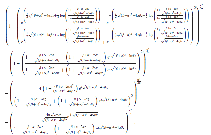 \begin{align*}&\left(1-\left(\frac{e^{\left(\frac{t}2 \sqrt{(\beta+\alpha)^2 - 4\alpha\beta z}+\frac{1}{2}\log\left(\frac{1 + \frac{ \beta+\alpha-2\alpha z}{\sqrt{(\beta+\alpha)^2 - 4\alpha\beta z}}}{1-\frac{ \beta+\alpha-2\alpha z}{\sqrt{(\beta+\alpha)^2 - 4\alpha\beta z}}}\right)\right)}-e^{-\left(\frac{t}2 \sqrt{(\beta+\alpha)^2 - 4\alpha\beta z}+\frac{1}{2}\log\left(\frac{1 + \frac{ \beta+\alpha-2\alpha z}{\sqrt{(\beta+\alpha)^2 - 4\alpha\beta z}}}{1-\frac{ \beta+\alpha-2\alpha z}{\sqrt{(\beta+\alpha)^2 - 4\alpha\beta z}}}\right)\right)}}{e^{\left(\frac{t}2 \sqrt{(\beta+\alpha)^2 - 4\alpha\beta z}+\frac{1}{2}\log\left(\frac{1 + \frac{ \beta+\alpha-2\alpha z}{\sqrt{(\beta+\alpha)^2 - 4\alpha\beta z}}}{1-\frac{ \beta+\alpha-2\alpha z}{\sqrt{(\beta+\alpha)^2 - 4\alpha\beta z}}}\right)\right)}+e^{-\left(\frac{t}2 \sqrt{(\beta+\alpha)^2 - 4\alpha\beta z}+\frac{1}{2}\log\left(\frac{1 + \frac{ \beta+\alpha-2\alpha z}{\sqrt{(\beta+\alpha)^2 - 4\alpha\beta z}}}{1-\frac{ \beta+\alpha-2\alpha z}{\sqrt{(\beta+\alpha)^2 - 4\alpha\beta z}}}\right)\right)}}\right)^2\right)^{\!\frac{\eta^*}{2\alpha}}\\&=\left(1-\left(\frac{1-\frac{ \beta+\alpha-2\alpha z}{\sqrt{(\beta+\alpha)^2 - 4\alpha\beta z}}-\left(1 + \frac{ \beta+\alpha-2\alpha z}{\sqrt{(\beta+\alpha)^2 - 4\alpha\beta z}}\right)e^{t \sqrt{(\beta+\alpha)^2 - 4\alpha\beta z}}}{1-\frac{ \beta+\alpha-2\alpha z}{\sqrt{(\beta+\alpha)^2 - 4\alpha\beta z}}+\left(1 + \frac{ \beta+\alpha-2\alpha z}{\sqrt{(\beta+\alpha)^2 - 4\alpha\beta z}}\right)e^{t \sqrt{(\beta+\alpha)^2 - 4\alpha\beta z}}}\right)^2\right)^{\!\frac{\eta^*}{2\alpha}}\\&=\left(\frac{4\left(1-\frac{ (\beta+\alpha-2\alpha z)^2}{(\beta+\alpha)^2 - 4\alpha\beta z}\right)e^{t \sqrt{(\beta+\alpha)^2 - 4\alpha\beta z}}}{\left(1-\frac{ \beta+\alpha-2\alpha z}{\sqrt{(\beta+\alpha)^2 - 4\alpha\beta z}}+\left(1 + \frac{ \beta+\alpha-2\alpha z}{\sqrt{(\beta+\alpha)^2 - 4\alpha\beta z}}\right)e^{t \sqrt{(\beta+\alpha)^2 - 4\alpha\beta z}}\right)^2}\right)^{\!\frac{\eta^*}{2\alpha}}\\&=\left(\frac{\frac{ 4\alpha \sqrt{z-z^2}}{\sqrt{(\beta+\alpha)^2 - 4\alpha\beta z}}e^{\frac{t}{2} \sqrt{(\beta+\alpha)^2 - 4\alpha\beta z}}}{1-\frac{ \beta+\alpha-2\alpha z}{\sqrt{(\beta+\alpha)^2 - 4\alpha\beta z}}+\left(1 + \frac{ \beta+\alpha-2\alpha z}{\sqrt{(\beta+\alpha)^2 - 4\alpha\beta z}}\right)e^{t \sqrt{(\beta+\alpha)^2 - 4\alpha\beta z}}}\right)^{\!\frac{\eta^*}{\alpha}}.\end{align*}
Finally, the third line of (54) is simplified through use of (52) and (53). This expression is then given by
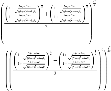 \begin{align*}&\left(\frac{\left(\frac{1 + \frac{2\alpha z - \beta - \alpha}{\sqrt{(\beta+\alpha)^2 - 4\alpha\beta z}}}{1-\frac{2\alpha z - \beta - \alpha}{\sqrt{(\beta+\alpha)^2 - 4\alpha\beta z}}}\right)^{\!\frac{1}{2}}+\left(\frac{1 - \frac{2\alpha z - \beta - \alpha}{\sqrt{(\beta+\alpha)^2 - 4\alpha\beta z}}}{1 + \frac{2\alpha z - \beta - \alpha}{\sqrt{(\beta+\alpha)^2 - 4\alpha\beta z}}}\right)^{\!\frac{1}{2}}}2\right)^{\!\frac{\eta^*}{\alpha}}\\& =\left(\left(\frac{\left(\frac{1 - \frac{\beta+\alpha-2\alpha z}{\sqrt{(\beta+\alpha)^2 - 4\alpha\beta z}}}{1+\frac{\beta+\alpha-2\alpha z}{\sqrt{(\beta+\alpha)^2 - 4\alpha\beta z}}}\right)^{\!\frac{1}{2}}+\left(\frac{1 + \frac{\beta+\alpha-2\alpha z}{\sqrt{(\beta+\alpha)^2 - 4\alpha\beta z}}}{1 - \frac{\beta+\alpha-2\alpha z}{\sqrt{(\beta+\alpha)^2 - 4\alpha\beta z}}}\right)^{\!\frac{1}{2}}}2\right)^2\right)^{\!\frac{\eta^*}{2\alpha}}\end{align*}
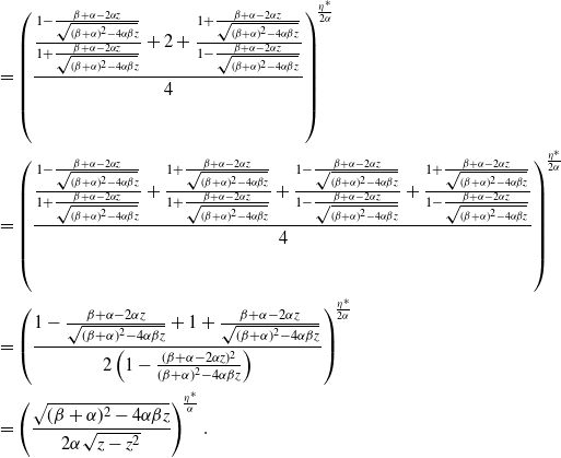 \begin{align*}&=\left(\frac{\frac{1 - \frac{\beta+\alpha-2\alpha z}{\sqrt{(\beta+\alpha)^2 - 4\alpha\beta z}}}{1+\frac{\beta+\alpha-2\alpha z}{\sqrt{(\beta+\alpha)^2 - 4\alpha\beta z}}}+2+\frac{1 + \frac{\beta+\alpha-2\alpha z}{\sqrt{(\beta+\alpha)^2 - 4\alpha\beta z}}}{1 - \frac{\beta+\alpha-2\alpha z}{\sqrt{(\beta+\alpha)^2 - 4\alpha\beta z}}}}4\right)^{\!\frac{\eta^*}{2\alpha}}\\&=\left(\frac{\frac{1 - \frac{\beta+\alpha-2\alpha z}{\sqrt{(\beta+\alpha)^2 - 4\alpha\beta z}}}{1+\frac{\beta+\alpha-2\alpha z}{\sqrt{(\beta+\alpha)^2 - 4\alpha\beta z}}}+\frac{1 + \frac{\beta+\alpha-2\alpha z}{\sqrt{(\beta+\alpha)^2 - 4\alpha\beta z}}}{1+\frac{\beta+\alpha-2\alpha z}{\sqrt{(\beta+\alpha)^2 - 4\alpha\beta z}}}+\frac{1 - \frac{\beta+\alpha-2\alpha z}{\sqrt{(\beta+\alpha)^2 - 4\alpha\beta z}}}{1-\frac{\beta+\alpha-2\alpha z}{\sqrt{(\beta+\alpha)^2 - 4\alpha\beta z}}}+\frac{1 + \frac{\beta+\alpha-2\alpha z}{\sqrt{(\beta+\alpha)^2 - 4\alpha\beta z}}}{1 - \frac{\beta+\alpha-2\alpha z}{\sqrt{(\beta+\alpha)^2 - 4\alpha\beta z}}}}4\right)^{\!\frac{\eta^*}{2\alpha}}\\&=\left(\frac{1 - \frac{\beta+\alpha-2\alpha z}{\sqrt{(\beta+\alpha)^2 - 4\alpha\beta z}}+1 + \frac{\beta+\alpha-2\alpha z}{\sqrt{(\beta+\alpha)^2 - 4\alpha\beta z}}}{2\left(1 - \frac{(\beta+\alpha-2\alpha z)^2}{(\beta+\alpha)^2 - 4\alpha\beta z}\right)}\right)^{\!\frac{\eta^*}{2\alpha}}\\&=\left(\frac{\sqrt{(\beta+\alpha)^2 - 4\alpha\beta z}}{ 2\alpha \sqrt{z-z^2}}\right)^{\!\frac{\eta^*}{\alpha}}.\end{align*}
Together these forms give the stated result.
Acknowledgements
We are grateful to Robert Hampshire, Emily Fischer, and Sam Gutekunst for helpful discussions. Publicly available drafts of this work used the moniker ‘Queue-Hawkes process’, but we have retitled to avoid confusion and ambiguity. Alas, ‘the process formerly known as the Queue-Hawkes’ is likely not an improvement in this regard.
Funding Information
We acknowledge the generous support of the National Science Foundation (NSF) through Andrew Daw’s Graduate Research Fellowship under grant DGE-1650441, received during his doctoral studies at Cornell University, when this research was initiated.
Competing Interests
There were no competing interests to declare which arose during the preparation or publication process for this article.


