

1. Introduction
Many industries face the problem of managing capacity in the face of unpredictably varying demand, e.g. adjusting the number of manufacturing lines to meet outstanding orders, determining the staffing levels at a call center, deploying webservers to handle internet traffic. To run a web site efficiently, for example, the recommended practice is to ‘match the number of servers to the current request volume’ (see the Amazon Web Services 2016 best practices available at https://docs.aws.amazon.com/opsworks/latest/userguide/best-practices-autoscale.html), but starting up and shutting down servers incurs separate costs. In this paper we study the problem of managing capacity based on the available workload. We model this as a generalization of a classic average cost Brownian control problem in which a system manager dynamically controls the drift rate of a diffusion process X. Whereas previous works constrained X to a finite interval via reflecting boundaries, the economic average cost Brownian control problem allows the controller to choose economic boundaries within a possibly infinite interval. At each instant, the system manager chooses the drift rate from a pair {u, v} of available rates and can invoke instantaneous controls either to keep X from falling or to keep it from rising. Under our model, instantaneous controls allow the controller to determine economic boundaries within the physical boundaries defining the maximum buffer size. The objective is to minimize the long-run average cost consisting of holding or delay costs proportional to X, processing costs proportional to the drift rate, costs for invoking instantaneous controls, and fixed costs for changing the drift rate. We impose no restrictions on the cost parameters.
The problem of controlling a Brownian motion by changing its drift rate has been studied at least since Bather (Reference Bather1968) cast the problem of controlling the output of a dam in terms of adjusting the drift rate of a Brownian motion. Since that time, many authors have explored the problem under a variety of cost functions and assumptions. See, for example, Ata, Harrison and Shepp (Reference Ata, Harrison and Shepp2005); Avram and Karaesmen (Reference Avram and Karaesmen1996); Chernoff and Petkau (Reference Chernoff and Petkau1978); Ghosh and Weerasinghe (Reference Ghosh and Weerasinghe2007); Perry and Bar-Lev (Reference Perry and Bar-Lev1989); Rath (Reference Rath1977); Ormeci Matoglu and Vande Vate (Reference Ormeci Matoglu and Vande Vate2011), and Wu and Chao (Reference Wu and Chao2014). Rath (Reference Rath1977) and Chernoff and Petkau (Reference Chernoff and Petkau1978) addressed a reflected Brownian motion process where the controller has a choice between two sets of drift and diffusion parameters while minimizing the long-run average cost consisting of changeover costs, processing costs, and delay or inventory holding costs. Chernoff and Petkau (Reference Chernoff and Petkau1978) encountered difficulties, due to a lack of compactness, in showing that policies satisfying the optimality conditions are optimal among all nonanticipating policies rather than just all stationary policies. They also observed that for problems involving more than two possible drift rates ‘the analytic approach becomes cumbersome’. Perry and Bar-Lev (Reference Perry and Bar-Lev1989) addressed a similar problem with two rates, but only considered a class of given policies. Subsequent investigations, including Ata et al. (Reference Ata, Harrison and Shepp2005) Harrison (Reference Harrison1985), Ghosh and Weerasinghe (Reference Ghosh and Weerasinghe2007), Liao (Reference Liao1984) and Perry and Bar-Lev (Reference Perry and Bar-Lev1989), overcome the compactness issues by requiring the controller to employ instantaneous controls to keep the process from exceeding a prescribed finite upper bound. In particular, Ata et al. (Reference Ata, Harrison and Shepp2005) solved a similar drift control problem that lives in a finite range, where the optimal negative drift rate is chosen to minimize the long-term average cost of control for drift and displacement at the upper boundary. They showed that the optimal drift rate is chosen in each state as a negative drift rate equal to the smallest minimizer of the Bellman equation they derived. A major difference between this work and our model is the lack of holding costs, changeover costs (the fixed cost for changing drift rate), and the fact that instantaneous controls are available only at the boundaries in Ata et al. (Reference Ata, Harrison and Shepp2005). Ghosh and Weerasinghe (Reference Ghosh and Weerasinghe2007) addressed the same problem, while also determining the optimal boundary (i.e. buffer size). Their model captured holding cost, but did not include changeover costs.Ghosh and Weerasinghe (Reference Ghosh and Weerasinghe2010) studied a similar problem with the added feature of impatient customers, and minimized the cost of abandonment, capacity, and rejected customers under the discounted cost criterion. Their model does not include holding and changeover costs. The changeover costs in our model, in some sense, make the controller liable for past decisions and result in an optimal policy that depends not only on the position of the process, but also on the current drift rate. Wu and Chao (Reference Wu and Chao2014) addressed a Brownian control problem under an average cost criterion with two drift rates and no instantaneous controls. Due to the lack of a finite upper bound, they focused on a class of admissible policies, and showed that the desired policy is optimal within this class of policies and that this class of policies is large enough to include most policies of practical interest. They considered a more general holding cost function, and a fixed changeover cost to turn on production, but did not include the cost of capacity. Ormeci Matoglu and Vande Vate (Reference Ormeci Matoglu and Vande Vate2011) and Ormeci Matoglu et al. (2005) developed methods for the problem with more than two drift rates that discretize the space of policies and refined the discretization to achieve ε-optimal solutions. These works allow only the controller to employ instantaneous controls at the system boundaries as required to keep the process within those boundaries.
In this paper we consider the problem with two drift rates, and adopt a slightly different cost model and available controls. Here, the controller must keep the process within prescribed, but possibly infinite boundaries, and is free to employ instantaneous controls at any time. This also allows the controller to determine economic boundaries within the physical boundaries defining the maximum buffer size. We assume linear cost functions, but impose no restrictions on the cost parameters.
We adapt the classical optimality conditions for two drift rates to the resulting drift control problem and show that a control band policy is optimal for the average cost problem under our cost model. In the process, we derive optimality conditions for the policy parameters and characterize conditions under which there is no lower bound on the average cost, a policy relying on a single drift rate is optimal or optimal policies employ both drift rates.
In Section 2 we describe the economic average cost Brownian control problem. In Section 3 we address the problem with one available drift rate. In Section 4 we extend our solution to the problem with two available drift rates. In Section 4.1 we solve the problem for the case in which there is no cost to change the drift rate and, in the process show how to solve this special case when there are more than two available drift rates. In Section 4.2 we show how to construct an optimal policy when the cost to change between two available drift rates is positive. For completeness and ease of reading, we present the main proofs in the body of the text, but relegate proofs of intermediate steps to the appendices. In Appendix D we provide expressions for computing the individual cost components and frequencies of controls under a given control band policy.
2. Brownian drift control problem
Let
 $$W(T) = W(0) + \int_0^T \mu (t) {\rm{d}}t + \sigma B(T),\quad \quad T \ge 0,$$
be a diffusion process with drift μ(t) ∈ {u,v}, variance σ2 > 0, and initial level W(0) on some filtered space
 $\{\Omega,\mathcal{F},\mathbb{P};\ \mathcal{F}_t,\,t\ge0\}$
. We assume that v > u and, to avoid tedious case analysis, we also assume that neither is 0. The process W(T) describes the difference between cumulative work to have arrived by time T and cumulative work processed by time T, i.e. the netput process. The drift rate {μ(t): t ≥ 0} is adapted to the Brownian motion {B(t): t ≥ 0}, and represents the difference between the average arrival rate and the rate at which work is completed.
$\{\Omega,\mathcal{F},\mathbb{P};\ \mathcal{F}_t,\,t\ge0\}$
. We assume that v > u and, to avoid tedious case analysis, we also assume that neither is 0. The process W(T) describes the difference between cumulative work to have arrived by time T and cumulative work processed by time T, i.e. the netput process. The drift rate {μ(t): t ≥ 0} is adapted to the Brownian motion {B(t): t ≥ 0}, and represents the difference between the average arrival rate and the rate at which work is completed.
The controller must exert the minimal instantaneous control required to keep the process within the prescribed range
 ${\mathcal{R = [0,}}\Theta ]$
if Θ > 0 is finite, or
${\mathcal{R = [0,}}\Theta ]$
if Θ > 0 is finite, or
 ${\mathcal{R = }}{{\mathbb{R}}_ + }$
if Θ is infinite, but may also invoke those controls at any time, e.g. by idling capacity or turning away work.
${\mathcal{R = }}{{\mathbb{R}}_ + }$
if Θ is infinite, but may also invoke those controls at any time, e.g. by idling capacity or turning away work.
We let A(T) denote the cumulative units of capacity lost to idling and let R(T) denote the cumulative amount of work turned away up to time T. The resulting controlled process is
 $$X(T) = X(0) + \int_0^T \mu (t) {\rm{d}}t + \sigma B(T) + A(T) - R(T),\quad \quad T \ge 0,$$
where X(0) = W(0). We assume, without loss of generality, that
 $W(0)\in \mathcal{R}$
and that μ(0) = u.
$W(0)\in \mathcal{R}$
and that μ(0) = u.
The controller incurs a cost of U per unit to idle capacity and a cost of M per unit to turn away customers, and must pay a fixed cost K(u, v) ≥ 0 to change the drift rate from u to v and a fixed cost K(v, u) ≥ 0 to change the drift rate from v to u. We let K = K(u, v)+K = (v, u).
When X(T) > 0, the backlog of work incurs a linear delay cost at rate h per unit time. The controller also incurs a cost per unit time for capacity that is linear in the drift rate. In particular, the cost for capacity when the drift rate is u is pu.
A policy defines the times at which to adjust the drift rate, idle capacity, and turn away work. We restrict attention to the space
 $\cal P$
of nonanticipating policies Φ = ({T i : i ≥ 0}, A, R), where
$\cal P$
of nonanticipating policies Φ = ({T i : i ≥ 0}, A, R), where
 $0 = T_0 \lt T_1 \lt T_2 \lt \ldots \lt T_i\lt T_{i+1} \lt \ldots $
is a sequence of stopping times, and
$0 = T_0 \lt T_1 \lt T_2 \lt \ldots \lt T_i\lt T_{i+1} \lt \ldots $
is a sequence of stopping times, andA and R are continuous, nondecreasing, adapted processes such that X as defined by (1) lies in
$\cal R$
for all T ≥ 0.


Under policy Φ = ({T i : i ≥ 0}, A, R), the drift rate μ(t) = μ i for T i ≤ t < T i+1, where μ 2i = u and μ 2i+1 = v for i ≥ 0.
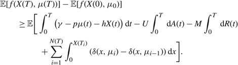
We consider the economic average cost Brownian control problem, which is to find a nonanticipating policy Φ = ({Ti : i ≥ 0}, A, R), that minimizes the long-run average cost:
 $${\rm{AC}}(\Phi ) = \mathop {\limsup }\limits_{T \to \infty } {1 \over T}\mathbb E \left[\int_0^T \left( {p\mu (t) + hX(t)} \right){\rm{d}}t + UA(T) + MR(T) + \sum\limits_{i = 1}^{N(T)} K({u_{i - 1}},{u_i}) \right].$$
Here, for each T ≥ 0, N(T) = sup{n ≥ 0: T n ≤ T} denotes the number of changes in the drift rate by time T.
We show that, when the economic average cost Brownian control problem admits an optimal policy, a control band policy is optimal. We characterize the conditions on the cost parameters under which there is no lower bound on the average cost, hence no optimal policy exists, and when an optimal policy exists, we determine optimal policy parameters.
Theorem 1
For the economic average cost Brownian control problem, the following statements hold.
(a) There is no lower bound when any of the following assertions hold.
M + U < 0,
h < 0 and Θ is infinite, or
h = 0, U < 0, and Θ is infinite.
(b) There is an optimal policy that simply exerts the minimal instantaneous control required to keep the process nonnegative when M + U ≥ 0, h = 0, U ≥ 0, and Θ is infinite. In this case an optimal policy relies on the faster drift rate v if p < U and on the slower drift rate u if p > U, and on either u or v if p = U.
(c) There is an optimal policy of the form (α, Ω), which dictates exerting minimum instantaneous control to keep the process between α and Ω, where 0 ≤ α ≤ Ω ≤ Θ, when M + U ≥ 0, Θ is finite if h ≤ 0, and either
p ≥ U, in which case the policy relies solely on the drift rate u,
–p ≥ M, in which case the policy relies solely on the drift rate v, or
- $K>\overline{K}$, a threshold defined by the problem parameters.
(d) There is an optimal policy of the form (α, s, Ω), where α and Ω with 0 ≤ α ≤ Ω ≤ Θ define the lower and upper limits on the process, and s with α ≤ s ≤ Ω defines the point at which to change the drift rate, when M > –U, Θ is finite if h ≤ 0 and K = 0. In this case, the policy relies on the slower drift rate u when the process exceeds s and on the faster drift rate v otherwise. The policy is optimal for the set {μ : u ≤ v} of available drift rates.
(e) There is an optimal policy of the form (α, S, Ω), where α and Ω with 0 ≤ α ≤ Ω ≤ Θ define the lower and upper limits on the process, and s and S with α ≤ s < S ≤ Ω define the points at which to change the drift rate, when M > –p > –U, Θ is finite if h ≤ 0 and
$\overline{K} \ge K \gt 0$. In this case, the policy maintains the slower drift rate u until the process falls below s and maintains the faster drift rate v until the process exceeds S.


In each case, an optimal policy is a control band policy.
In this context, a control band policy Φ is defined as a pair of bands, Φ = {ϕu, ϕv}, where ϕμ = (μ, sμ, βμ, Sμ, τμ). Under the control band policy Φ, the controller maintains the drift rate μ and refrains from intervention so long as X remains in the interval (sμ, Sμ). When X reaches sμ, the value β μ ∈ {u, v} indicates the appropriate action. If β μ = μ, the controller exerts instantaneous controls, i.e. idles capacity to keep X ≥ s μ. Otherwise, the controller changes the drift rate. Similarly, when X reaches Sμ, τ μ ∈ {u, v} indicates the appropriate action. If τ μ = μ, the controller exerts instantaneous controls, i.e. turns away work to keep X ≤ Sμ. Otherwise, the controller changes the drift rate. Note that, when there is only one available drift rate μ, a control band policy is equivalent to setting bounds on the buffer size. In this case, the controller may set sμ > 0 and/or Sμ < Θ for economic reasons, or set sμ = 0 and Sμ = Θ to exploit the full physical capacity available.
We prove Theorem 1(a) in Lemma 1 and Lemma 2 of Section 3. We prove Theorem 1(b) in Lemma 2 of Section 3. We prove Theorem 1(c) in Lemma 4 of Section 4 and Corollary 9 of Section 4.2. We prove Theorem 1(d) in Lemma 10 and Corollary 8 of Section 4.1. We prove Theorem 1(e) in Section 4.2. In Appendix D we provide detailed performance metrics for policies of the forms (α, Ω) (α, s, Ω), and (α, s, S, Ω).
3. The one-drift rate problem: economic bounds
We first consider the case of a single drift rate μ in which the controller can only employ instantaneous controls. In the classic setting, the only possible policy is to idle capacity when the buffer is empty and turn away work when the buffer reaches the prescribed limit Θ. The economic average cost problem modifies this classic problem in two ways. First, it allows the prescribed upper bound Θ to be infinite and, second, it allows the controller to employ instantaneous controls at any time. Harrison and Taksar (Reference Harrison and Taksar1983) addressed the problem of using instantaneous controls to manage a Brownian motion within a compact state space, under a discounted cost setting with nonnegative convex holding costs, and Dai and Yao (Reference Dai and Yao2013) studied average cost Brownian control problems with instantaneous and impulse controls under nonnegative convex holding costs on the real line. We extend Dai and Yao (Reference Dai and Yao2013) by considering possibly negative (but linear holding costs) and possibly negative costs for instantaneous controls. We identify when the problem has a solution and provide closed-form expressions for an optimal policy and its average cost when such a policy exists.
Since the actions β and τ are fully determined in the one-drift rate problem, a control band in this context reduces to a pair (α, Ω), where 0 ≤ α < Ω ≤ Θ.
Observe that, for any policy
 $\Phi_0 = \{A_0, R_0\} \in \mathcal{P}$
, the policy Φ
a
= {A a, R a}, where A a (T) = A 0 (T) + aT and R a (T) = R 0 (T) + aT, is also in
$\cal P$
and AC(Φ
a
) = AC(Φ0)+ (M + U)a. Thus, we see that if M + U < 0, there is no lower bound on the average cost of a policy.
$\Phi_0 = \{A_0, R_0\} \in \mathcal{P}$
, the policy Φ
a
= {A a, R a}, where A a (T) = A 0 (T) + aT and R a (T) = R 0 (T) + aT, is also in
$\cal P$
and AC(Φ
a
) = AC(Φ0)+ (M + U)a. Thus, we see that if M + U < 0, there is no lower bound on the average cost of a policy.
The policy Φ a involves a bit of ‘cheating’: the controller is rejecting work that has not yet arrived in order to idle additional capacity. This phenomenon highlights a strong connection between A and R that we formalize and exploit in Proposition 2.
Lemma 1
If M + U < 0, there is no lower bound on the average cost of a policy.
In the remainder of the paper we adopt the following assumption.
Assumption 1
It holds that M + U ≥ 0.
Proposition 1 provides weak lower bounds on the average cost of any nonanticipating policy.
Proposition 1
Suppose that the scalar γ and the continuous function
 $\delta\colon \mathcal{R}\to \mathbb{R}$
satisfy the following conditions:
$\delta\colon \mathcal{R}\to \mathbb{R}$
satisfy the following conditions:
 $$\delta (x) \;is\;continuously\;differentiable\;except\;at\;a\;finite\;set\;of\;points\;in\; {\cal R},$$
 $${{{\sigma ^2}} \over 2}{\delta ^{'}}(x) + \mu \delta (x) + p\mu + hx \ge \gamma \quad for\;almost\;all\; x \in {\cal R},$$
 $$ - U \le \delta (x) \le \min \{ 0,M\} \quad for\;all\; x \in \cal R.$$
Then γ ≤ AC(Φ) for each policy
 $\Phi \in \mathcal{P}$
.
$\Phi \in \mathcal{P}$
.
Proof. The proof follows from an application of Itô’s formula. (Itô’s formula for semimartingales can be found, for example, in Theorem I.4.57 of Jacod and Shiryaev (Reference Jacod and Shiryaev2003).) Suppose that f:
 $\cal R \to \mathbb R$
is continuously differentiable, has a bounded derivative, and has a continuous second derivative at all but a finite number of points. Then, for each time T > 0, initial state X(0), and policy
$\cal R \to \mathbb R$
is continuously differentiable, has a bounded derivative, and has a continuous second derivative at all but a finite number of points. Then, for each time T > 0, initial state X(0), and policy
 $\Phi=\{A,R\}\in\mathcal{P},$
we have
$\Phi=\{A,R\}\in\mathcal{P},$
we have
 $$f(X(T)) = f(X(0)) + \int_0^T {f^{'}}(X(t)) {\rm{d}}X(t) + {1 \over 2}\int_0^T {f^{''}}(X(t)) {\rm{d}}X(t) {\rm{d}}X(t),$$
where
 $${\rm{d}}X(t) = \mu {\rm{d}}t + \sigma {\rm{d}}B(t) + {\rm{d}}A(t) - {\rm{d}}R(t)\quad {\rm{and}}\quad {\rm{d}}X(t) {\rm{d}}X(t) = {\sigma ^2} {\rm{d}}t.$$
Hence,
 $$\eqalign{ {\mathbb{E}}[f(X(T))] & = {\mathbb{E}}[f(X(0))] + {\mathbb{E}}[\int_0^{T} ({{{\sigma ^{2}}} \over 2}{f^{''}}(X(t)) + \mu {f^{'}}(X(t))) {\rm{d}}t \cr & + \int_0^T {f^{'}}(X(t)) {\rm{d}}A(t) - \int_0^T {f^{'}}(X(t)) {\rm{d}}R(t)]. } $$
When
 $f(x) = \int_0^x \delta (\xi ) {\rm{d}}\xi $
so that
$f(x) = \int_0^x \delta (\xi ) {\rm{d}}\xi $
so that
 ${f^{'}}(x) = \delta (x)$
, the inequalities (3) and (4) yield
${f^{'}}(x) = \delta (x)$
, the inequalities (3) and (4) yield
 $$\eqalign{ {\mathbb{E}}[f(X(T))] & - {\mathbb{E}}[f(X(0))] \cr & {= {\mathbb{E}}[\int_0^{T} ({{{\sigma ^{2}}} \over 2}{\delta ^{'}}(X(t)) + \mu \delta (X(t))) {\rm{d}}t + \int_0^{T} \delta (X(t))dA(t) - \int_0^{T} \delta (X(t)) {\rm{d}}R(t)]} \cr & \ge {\mathbb{E}}[\int_0^T (\gamma - p\mu - hX(t)) {\rm{d}}t - U\int_0^{T} {\rm{d}}A(t) - M\int_0^{T} {\rm{d}}R(t)].} $$
Rearranging terms, dividing both sides by T, and taking the limit superior as T goes to ∞ we see that
 $$\eqalign{ & \mathop {\limsup }\limits_{T \to \infty } {1 \over T}({\mathbb{E}}[f(X(T))] - {\mathbb{E}}[f(X(0))]) \cr & + \mathop {\limsup }\limits_{T \to \infty } {1 \over T}{\mathbb{E}}[\int_0^T (p\mu + hX(t)) {\rm{d}}t + U\int_0^T {\rm{d}}A(t) + M\int_0^T {\rm{d}}R(t)] \cr & \quad \quad = \mathop {\limsup }\limits_{T \to \infty } {1 \over T}({\mathbb{E}}[f(X(T))] - {\mathbb{E}}[f(X(0))]) + {\rm{AC}}(\Phi ) \cr & \quad \quad \ge \gamma . \cr} $$
The fact that δ(x) ≤ 0 for
 $x\in\mathcal{R}$
implies that f (x) ≤ f (0) for
$x\in\mathcal{R}$
implies that f (x) ≤ f (0) for
 $x\in \mathcal{R}$
, and so
$x\in \mathcal{R}$
, and so
 $$\mathop {\limsup }\limits_{T \to \infty } {1 \over T}({\mathbb{E}}[f(X(T))] - {\mathbb{E}}[f(X(0))]) \le 0,$$
proving that γ ≤ AC(Φ).
Lemma 2 exploits the arguments of Proposition 1 to construct an optimal control band policy (α, Ω) or prove that no optimal policy exists when h ≤ 0 and Θ is infinite.
Lemma 2
Under Assumption 1, when Θ is infinite,
(a) if h < 0, limα→∞ AC(α, α + 1) = –∞ and so there is no lower bound on the average cost of a policy;
(b) if h = 0 and U ≥ 0 then
(b.1) if μ < 0 (μ < 0) is an optimal policy and AC(0, ∞) = (p – U)μ;
(b.2) if μ > 0 and M ≥ 0 (0, ∞) is an optimal policy and AC(0, ∞) = pμ;
(b.3) if μ > 0 and M < 0 (0, ∞) is an optimal policy and AC(0, ∞) = (M + p)μ;
(c) if h = 0 and U < 0 then there is no lower bound on the average cost of a policy.
Proof. Case (a): h < 0. Observe that (see Lemma 13 in Appendix D)
 $${\rm{AC}}(\alpha ,\alpha + 1) = {{(M + p)\mu + {{\mathbb{E}}^{ - 2\mu /{\sigma ^2}}}(U - p)\mu + h} \over {1 - {{\mathbb{E}}^{ - 2\mu /{\sigma ^2}}}}} - {{h{\sigma ^2}} \over {2\mu }} + h\alpha ,$$
and so, when h < 0 and Θ is infinite,
 $$\mathop {\lim }\limits_{\alpha \to \infty } {\rm{AC}}(\alpha ,\alpha + 1) = - \infty $$
and there is no lower bound on the average cost of a policy.
In the other cases, we consider
 $${\rm EA}(0,\Omega ) = {\mu \over {{{\rm e}^{2\mu \Omega /{\sigma ^2}}} - 1}}\quad {\rm{and}}\quad {\rm ER}(0,\Omega ) = {\mu \over {1 - {{\rm e}^{ - 2\mu \Omega /{\sigma ^2}}}}},$$
the average rates of instantaneous control at 0 and at Ω, respectively, under the policy (0, Ω) for Ω positive and finite. (See Lemma 13 in Appendix D.)
Case (b.1): h = 0, U ≥ 0, and μ < 0. Observe that δ(x) = –U and γ = (p – U) μ satisfy the conditions of Proposition 1, proving that (p – U) μ is a lower bound on the average cost of any nonanticipating policy. In this case, the fact that limΩ→∞ EA(0, Ω) = –μ implies that AC(0, Ω) = pμ + UEA(0, ∞) = (p – U) μ , proving that (0, ∞) is an optimal policy.
Case (b.2) h = 0, U ≥ 0, M ≥ 0, and μ > 0. Since M ≥ 0 ≥ –U, δ(x) = 0, and γ = pμ satisfy the conditions of Proposition 1, proving that pμ is a lower bound on the average cost of any nonanticipating policy. In this case, the fact that limΩ→∞ EA(0, Ω) = 0 implies that limΩ→∞ AC(0, Ω) = pμ, proving that (0, ∞) is an optimal policy.
Case (b.3) h = 0, U ≥ 0, M < 0, and μ > 0. Observe that δ(x) = M and γ = (M + p)μ satisfy the conditions of Proposition 1, proving that (M + p)μ is a lower bound on the average cost of any nonanticipating policy. In this case, the facts that limΩ→∞ EA(0, Ω) = 0 and limΩ→∞ EA(0, Ω) = –μ limΩ→∞ ER(0, Ω) = μ imply that limΩ→∞ AC(0, Ω) = (M + p)μ, proving that, as Ω goes to ∞, the policy (0, Ω) is optimal.
Case (c). h = 0 and U < 0. Consider the policy Φ = {A, R} with R(T) = 0 and A(T) = A 0(T)+ aT for each T ≥ 0, where A 0 is the minimal instantaneous control required at 0 to keep the process non-negative and a > 0 is essentially a positive drift induced by additional instantaneous controls at every point. When U < 0 and h = 0,
 $${\rm{AC}}(\Phi ) = \mathop {\limsup }\limits_{T \to \infty } {1 \over T}{\mathbb{E}} \left[\int_0^T p\mu {\rm{d}}t + U{A_0}(T) + UaT \right] \le p\mu + aU,$$
and, by making a large the controller can drive the average cost to –∞, proving that the problem has no lower bound.
Lemma 2 shows that when h ≤ 0 and Θ is infinite, the one-drift rate economic average cost problem either admits no best policy or a best policy is essentially for the controller to exert only the minimum effort required to keep the process nonnegative. To focus attention on the more interesting cases, in the remainder of the paper we adopt the following assumption.
Assumption 2
If h ≤ 0 then Θ is finite.
Under Assumption 2, Proposition 2 provides stronger lower bounds on the average cost of any nonanticipating policy for the one-drift rate economic average cost problem.
Proposition 2
Under Assumptions 1 and 2, suppose that the scalar γ and the continuous function
$\delta\colon \mathcal{R}\to \mathbb{R}$
satisfy (2)–(3) and
 $$ - U \le \delta (x) \le M\quad \;for\;all\; x \in {\cal R}.$$
Then γ ≤ AC(Φ) for each policy
 $\Phi \in \mathcal{P}$
.
$\Phi \in \mathcal{P}$
.
Corollary 1 summarizes useful bounds obtained from simple applications of Proposition 2.
Corollary 1
Under Assumptions 1 and 2,
 $${\rm{AC}}(\Phi ) \ge \left \{ \matrix{ {\max \{ (M + p)\mu , - (U - p)\mu \} } \hfill & {{if}\;h \ge 0,} \hfill \cr {\max \{ - (U - p)\mu + h\Theta ,(M + p)\mu + h\Theta \} } \hfill & {{if}\;h \lt 0,}}\right. $$
for each policy
 $\Phi\in\mathcal{P}$
.
$\Phi\in\mathcal{P}$
.
Proof. When h ≥ 0, the function δ(x) = M and the scalar γ = (M + p)μ satisfy the conditions of Proposition 2. Similarly, the function δ(x) = –U and the scalar γ = –(U – p)μ satisfy the conditions of Proposition 2. When h < 0, the function δ(x) = –U and the scalar γ = –(U – p)μ + hΘ satisfy the conditions of Proposition 2. Similarly, the function δ(x) = M and the scalar γ = (M + p)μ + hΘ satisfy the conditions of Proposition 2.
We employ Proposition 2 and Corollary 2 to construct an optimal control band policy (α, Ω) with the interpretation that the controller should idle capacity to keep X ≥ α and turn away work to keep X ≤ Ω. The proof of Proposition 2 is presented after Corollary 2.
Corollary 2
Under Assumptions 1 and 2, suppose that 0 ≤ α < Ω ≤ Θ, and that the scalar γ and the continuous function
 $\delta(x)\colon \mathcal{R}\to\mathbb{R}$
satisfy (2)–(3) and (6). If γ and δ also satisfy
$\delta(x)\colon \mathcal{R}\to\mathbb{R}$
satisfy (2)–(3) and (6). If γ and δ also satisfy
 $${{{\sigma ^2}} \over 2}{\delta ^{'}}(x) + \mu \delta (x) + p\mu + hx = \gamma \quad for\;almost\;all\; x \in [\alpha ,\Omega ],$$
 $$\delta (\alpha ) = - U,$$
 $${\rm{and}}\;\delta (\Omega ) = M\quad if\;\Omega \;is\;finite ,$$
then AC(α, Ω) = γ, and so (α, Ω) is an optimal policy.
Proof of Proposition 2. The proof is analogous to the proof of Proposition 1. Under Assumption 2, we prove that, when
 $$a = \mathop {\liminf}\limits_{T \to \infty } {1 \over T}({\mathbb{E}}[f(X(T))] - {\mathbb{E}}[f(X(0))])$$
is positive, AC(Φ) = ∞ and so AC(Φ) ≥ γ trivially.
When f (x) = x (5) becomes
 $${\mathbb{E}}[X(T)] = {\mathbb{E}}[X(0)] + \mu T + {\mathbb{E}}[A(T)] - {\mathbb{E}}[R(T)].$$
When
 $f(x) = \int_0^x \delta (\xi ) {\rm{d}}\xi $
so that
$f(x) = \int_0^x \delta (\xi ) {\rm{d}}\xi $
so that
 $f^\prime(x)=\delta(x)$
, inequalities (3) and (6) yield
$f^\prime(x)=\delta(x)$
, inequalities (3) and (6) yield
 $$\eqalign{ & {\mathbb{E}}[f(X(T))] - {\mathbb{E}}[f(X(0))] \cr & \quad \quad = {\mathbb{E}}\left[\int_0^T ({{{\sigma ^2}} \over 2}{\delta ^{'}}(X(t)) + \mu \delta (X(t))) {\rm{d}}t + \int_0^{T} \delta (X(t)) {\rm{d}}A(t) - \int_0^{T} \delta (X(t)) {\rm{d}}R(t) \right] \cr & \quad \quad \ge {\mathbb{E}} \left[\int_0^{T} (\gamma - p\mu - hX(t)) {\rm{d}}t - U\int_0^{T} {\rm{d}}A(t) - M\int_0^{T} {\rm{d}}R(t) \right].} $$
Dividing both sides by T and taking the limit inferior as T goes to ∞, using the relationship lim inf (–A) = – lim sup (A) and rearranging terms, we see that
 $$\eqalign{ & \mathop {\liminf}\limits_{T \to \infty } {1 \over T}({\mathbb{E}}[f(X(T))] - {\mathbb{E}}[f(X(0))]) \cr & + \mathop {\limsup }\limits_{T \to \infty } {1 \over T}{\mathbb{E}} \left[\int_0^T (p\mu + hX(t)) {\rm{d}}t + U\int_0^T {\rm{d}}A(t) + M\int_0^T {\rm{d}}R(t) \right] \cr & \quad \quad \ge \gamma .} $$
Let
 $$a = \mathop {\liminf}\limits_{T \to \infty } {1 \over T}({\mathbb{E}}[f(X(T))] - {\mathbb{E}}[f(X(0))]).$$
If a ≤ 0 (11) implies that AC(Φ) ≥ γ. If a > 0, observe that, since it has bounded derivative, f is Lipschitz continuous and there exists a constant r > 0 such that
 $$f(X(T)) - f(X(0)) \le |f(X(T)) - f(X(0))| \le r|(X(T) - X(0)| \le r(X(T) + X(0))$$
for all T ≥ 0 and
 $$0 \lt a = \mathop {\liminf}\limits_{T \to \infty } {1 \over T}{\mathbb{E}}[f(X(T))] \le \mathop {\liminf}\limits_{T \to \infty } {1 \over T}r{\mathbb{E}}[(X(T) + X(0))] = \mathop {\liminf}\limits_{T \to \infty } {r \over T}{\mathbb{E}}[X(T)].$$
Thus, there exists a constant b ≥ a/r such that
 $$0 \lt b = \mathop {\liminf}\limits_{T \to \infty } {1 \over T}{\mathbb{E}}[X(T)]$$
and a constant t* > 0 such that
 $${\mathbb{E}}[X(T)] \gt {b \over 2}T\quad {\rm for}\;{\rm all}\; T \gt {t^*}.$$
The fact that .
 ${\mathbb{E}}[X(T)]$
has no upper limit implies that Θ must be infinite and so, by Assumption 2, h > 0. Thus, by Tonelli’s theorem,
${\mathbb{E}}[X(T)]$
has no upper limit implies that Θ must be infinite and so, by Assumption 2, h > 0. Thus, by Tonelli’s theorem,
 $$\eqalign{ \mathop {\liminf}\limits_{T \to \infty } {1 \over T}{\mathbb{E}} [\int_0^T hX(t) {\rm{d}}t] & = \mathop {\liminf}\limits_{T \to \infty } {1 \over T}\int_0^T h{\mathbb{E}}\left[ {X(t)} \right] {\rm{d}}t \cr & \ge \mathop {\liminf}\limits_{T \to \infty } {1 \over T}\int_{{t^*}}^T h{b \over 2}t {\rm{d}}t \cr & = \mathop {\liminf}\limits_{T \to \infty } {{hb} \over 4}{{{T^2} - {t^{*2}}} \over T} \cr & = \infty .} $$
Furthermore, by (10)
 $$\eqalign{{1 \over T}\left( {U{\mathbb{E}}[A(T)] + M{\mathbb{E}}[R(T)]} \right) & = {1 \over T}U({\mathbb{E}}[X(T)] - {\mathbb{E}}[X(0)]) - U\mu + {1 \over T}\left( {M + U} \right){\mathbb{E}}[R(T)] \cr & \ge {1 \over T}U({\mathbb{E}}[X(T)] - {\mathbb{E}}[X(0)]) - U\mu ,} $$
where the last inequality follows from Assumption 1. Taking the limit inferior as T → ∞ yields
 $$\eqalign{ & \mathop {\liminf}\limits_{T \to \infty } {1 \over T}\left( {U{\mathbb{E}}[A(T)] + M{\mathbb{E}}[R(T)]} \right) \cr & \quad \quad \ge \mathop {\liminf}\limits_{T \to \infty } ({1 \over T}U({\mathbb{E}}[X(T)] - {\mathbb{E}}[X(0)]) - U\mu ) \cr & \quad \quad \ge \mathop {\liminf}\limits_{T \to \infty } {1 \over T}U{\mathbb{E}}[X(T)] + \mathop {\liminf}\limits_{T \to \infty } {1 \over T}U( - {\mathbb{E}}[X(0)]) + \mathop {\liminf}\limits_{T \to \infty } ( - U\mu ) \cr & \quad \quad = U(b - \mu ). \cr} $$
Thus,
 $${\rm{AC}}(\Phi ) \ge p\mu + U (b - \mu ) + \mathop {\liminf}\limits_{T \to \infty } {{hb} \over 4}{{{T^2} - {t^{*2}}} \over T} = p\mu + b\mathop {\liminf}\limits_{T \to \infty } ({h \over 4}T + U) = \infty .$$
Corollary 2 follows from the fact that, for a control band policy (α, Ω), with Ω finite, there is a unique smooth function g and a unique constant γ that satisfy (7)–(9) and AC(α, Ω) = γ. In particular (7) has the general solution
 $$g(x) = - p - {{hx} \over \mu } + {{h{\sigma ^2}} \over {2{\mu ^2}}} + {\gamma \over \mu } + {{\rm e}^{ - 2\mu x/{\sigma ^2}}}{C_\mu },$$
for some constant C μ, and (8) implies that
 $${C_\mu } = - {{\rm e}^{2\mu \alpha /{\sigma ^2}}}(U - p + {{h{\sigma ^2}} \over {2{\mu ^2}}} + {\gamma \over \mu } - {{h\alpha } \over \mu }).$$
When Ω is finite, (9) implies that
 $${C_\mu } = {{\mathbb{E}}^{2\mu \Omega /{\sigma ^2}}}(M + p - {{h{\sigma ^2}} \over {2{\mu ^2}}} - {\gamma \over \mu } + {h \over \mu }\Omega )$$
and (12)–(13) uniquely determine the average cost γ and the scalar Cμ as functions of the control parameters (α, Ω):
 $$\eqalign{ & {\gamma _\mu }(\alpha ,\Omega ) \cr & = {{{{\rm e}^{2\mu \Omega /{\sigma ^2}}}(h\Omega - h{\sigma ^2}/(2\mu ) + \mu (M + p)) - {{\rm e}^{2\mu \alpha /{\sigma ^2}}}(\alpha h - h{\sigma ^2}/(2\mu ) - \mu (U - p))} \over {{{\rm e}^{2\mu \Omega /{\sigma ^2}}} - {{\rm e}^{2\mu \alpha /{\sigma ^2}}}}}, \cr & \quad \quad \quad \quad \quad \quad \quad \quad \quad {C_\mu }(\alpha ,\Omega ) = {{h(\Omega - \alpha ) + (M + U)\mu } \over {({{\rm e}^{ - 2\mu \Omega /{\sigma ^2}}} - {{\rm e}^{ - 2\mu \alpha /{\sigma ^2}}})\mu }}.} $$
Lemma 3 and Lemma 4 provide explicit formulae for the parameters of an optimal control band policy under Assumptions 1 and 2. These computations rely on the Lambert-W functions Wk(⋅), where Wk(⋅) is the kth branch of the inverse relation for the function f (w) = wew defined on the complex field (see, for example, Corless et al. (Reference Corless, Gonnet, Hare and Knuth1996), Euler (Reference Euler1921) and Lambert (Reference Lambert1758, Reference Lambert1772)). For each real value w with –1/e < w < 0, there are two possible real values for W(w), one on the branch W –1(⋅)with W –1(w) < –1 and the other on the branch W0 (⋅) with W 0(w) > –1.
Given 0 ≤ α < Ω ≤ Θ, where Ω is finite, we define
 $${g_{(\alpha ,\Omega )}}(x) = - p - {{hx} \over \mu } + {{h{\sigma ^2}} \over {2{\mu ^2}}} + {{{\gamma _\mu }(\alpha ,\Omega )} \over \mu } + {{\rm e}^{ - 2\mu x/{\sigma ^2}}}{C_\mu }(\alpha ,\Omega )$$
and so
 $$g_{(\alpha ,\Omega )}^{'}(x) = - {h \over \mu } - {{2\mu } \over {{\sigma ^2}}}{{\rm e}^{ - 2\mu x/{\sigma ^2}}}{C_\mu }(\alpha ,\Omega ) = - {h \over \mu } - {2 \over {{\sigma ^2}}}{{h(\Omega - \alpha ) + (M + U)\mu } \over {{{\rm e}^{ - 2\mu (\Omega - x)/{\sigma ^2}}} - {{\rm e}^{ - 2\mu (\alpha - x)/{\sigma ^2}}}}}.$$
Lemma 3
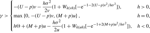
Under Assumptions 1 and 2, when h > 0, the unique nonnegative solution to the equation
 $$g_{(0,z)}^{'}(z) = 0$$
is
 $${\Omega ^*}(\mu ) = - {{(M + U)\mu } \over h} - {{{\sigma ^2}} \over {2\mu }}(1 + {W_{k(h\mu )}}( - {{\rm e}^{ - 1 - 2(M + U){\mu ^2}/h{\sigma ^2}}})),$$
where k(x) = 0 if x < 0 and k(x) = –1 if x > 0. When h < 0, the unique solution to
 $g_{(z,\Theta )}^{'}(z) = 0$
satisfying z ≤ Θ is given by
$g_{(z,\Theta )}^{'}(z) = 0$
satisfying z ≤ Θ is given by
 $${\alpha ^*}(\mu ) = \Theta + {{(M + U)\mu } \over h} - {{{\sigma ^2}} \over {2\mu }}(1 + {W_{k(h\mu )}}( - {{\rm e}^{ - 1 + 2(M + U){\mu ^2}/h{\sigma ^2}}})).$$
The proof of Lemma 3 is given in Appendix A.
Observe that, by definition,
 $$\eqalign{ & {\alpha ^*}(\mu ) = {{{\gamma _\mu }({\alpha ^*}(\mu ),\Theta ) + (U - p)\mu } \over h}\quad {\rm when}\;h \lt 0, \cr & {\Omega ^*}(\mu ) = {{{\gamma _\mu }(0,{\Omega ^*}(\mu )) - (M + p)\mu } \over h}\quad {\rm when}\; h \gt 0. \cr} $$
Lemma 4 shows how to construct an optimal policy from these points.
Lemma 4
Under Assumptions 1 and 2, the control band policy (αμ, Ωμ), where
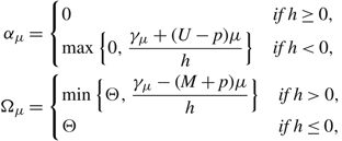
 $${\alpha _\mu } = \left\{ {\matrix{ 0 & { if\; h \ge 0,} \cr {\max \{ 0,{\alpha ^*}(\mu )\} } & { if\; h \lt 0,} \cr } } \right.$$
and
 $${\Omega _\mu } = \left\{ {\matrix{ {\min \{ \Theta ,{\Omega ^*}(\mu )\} } & { if\; h \gt 0,} \cr \Theta & { if\; h \le 0,} \cr } } \right.$$
and α* (μ) and Ω* (μ) are defined by (17) and (16), respectively, is an optimal policy.
Observe that the fact that an optimal policy prescribes setting α = 0 when h > 0 and Ω = Θ when h < 0 follows intuitively, as, when h < 0, raising the upper limit of the process increases the savings from negative holding costs and reduces the frequency of instantaneous controls. Similarly, when h < 0, reducing the lower limit reduces both the holding costs and the frequency of instantaneous controls. We provide a formal proof below.
Proof. To simplify notation, let α = αμ and Ω = Ωμ. For each finite α and Ω with 0 < Ω ≤ Θ and 0 ≤ α < Ω, define
 $${\delta _{(\alpha ,\Omega )}}(x) = \left\{ {\matrix{ { - U,} & {0 \le x \lt \alpha ,} \cr {{g_{(\alpha ,\Omega )}}(x),} & {\alpha \le x \le \Omega ,} \cr {M,} & {\Omega \lt x.} } } \right.$$
We argue that δ (α, Ω), where α and Ω are defined by (19) and (20), respectively, satisfies all the conditions of Corollary 2. We present the proof for the h > 0 case. The proof for the h ≤ 0 case is analogous, but relies on an assumption that Θ is finite in this case.
When h > 0, Ω is finite, and δ = δ (α, Ω) and γ = γμ (α, Ω) satisfy (7)–(9) by construction. It remains to show that δ and γ satisfy (2) (3), and (6) as well.
To see that (6) holds, note that
 $$g_{(0,{\Omega ^*}(\mu ))}^{''}(x) = {{4{\mu ^2}} \over {{\sigma ^4}}}{C_\mu }(0,{\Omega ^*}(\mu )){{\rm e}^{ - 2\mu x/{\sigma ^2}}},$$
 $${C_\mu }(0,{\Omega ^*}(\mu )) = - {{h{\sigma ^2}} \over {2{\mu ^2}}}{{\rm e}^{2\mu {\Omega ^*}(\mu )/{\sigma ^2}}} \lt 0,$$
proving that g = g (0,Ω*(μ)) is concave and increasing on [0, Ω*(μ)). We consider the two cases Ω*(μ) ≤ Θ and Ω*(μ) ≤ Θ separately.
Case (i): Ω*(μ) ≤ Θ. In this case the facts that g (Ω*(μ)) = M and
 ${g^{'}}({\Omega ^*}(\mu )) = 0$
ensure that δ is continuous and indeed continuously differentiable on
${g^{'}}({\Omega ^*}(\mu )) = 0$
ensure that δ is continuous and indeed continuously differentiable on
 $\mathcal{R}$
. Furthermore, since g is increasing on [0, Ω*(μ)) and satisfies g(0) = –U and g(Ω*(μ)) = M by construction, we see that δ satisfies (6).
$\mathcal{R}$
. Furthermore, since g is increasing on [0, Ω*(μ)) and satisfies g(0) = –U and g(Ω*(μ)) = M by construction, we see that δ satisfies (6).
Finally, we show that δ and γ satisfy (3). Note that, by construction, g and γ satisfy (3) with equality for 0 ≤ x ≤ Ω*(μ). By (18), (3) reduces to (M + p)μ + hx ≥ γ = (M + p)μ + Ω*(μ) for Ω*(μ) < x and, since h > 0, we see that δ and γ satisfy (3) for Ω*(μ) < x as well.
Case (ii): Ω*(μ) > Θ. In this case δ = g(0, Θ) on
 $\mathcal{R},$
and so is continuous and satisfies (2), and δ and γ satisfy (3) by construction. It remains only to show that δ satisfies (6).
$\mathcal{R},$
and so is continuous and satisfies (2), and δ and γ satisfy (3) by construction. It remains only to show that δ satisfies (6).
Observe that, since δ(0) = –U < M = δ(Θ), if
 $\delta^\prime $
has no root in
$\delta^\prime $
has no root in
 $\mathcal{R}$
then δ must be increasing on
$\mathcal{R}$
then δ must be increasing on
 $\mathcal{R}$
and so δ satisfies (6). If
$\mathcal{R}$
and so δ satisfies (6). If
 $\delta^\prime$
has a real root x
* then
$\delta^\prime$
has a real root x
* then
 $${\delta ^{'}}({x^*}) = - {h \over \mu } - {{2\mu } \over {{\sigma ^2}}}{{\rm e}^{ - 2\mu {x^*}/{\sigma ^2}}}{C_\mu }(0,\Theta ) = 0,$$
and so
 $${C_\mu }(0,\Theta ) = {{h\Theta + (M + U)\mu } \over {({{\rm e}^{ - 2\mu \Theta /{\sigma ^2}}} - 1)\mu }} = - {{h{\sigma ^2}} \over {2{\mu ^2}}}{{\rm e}^{2\mu {x^*}/{\sigma ^2}}} \lt 0$$
and δ is concave. Furthermore, since (e–2μΘ/σ2 –1)μ < 0,
 $$h\Theta + (M + U) \mu \gt 0.$$
We argue that x
* > Θ and so δ is increasing on
 $\mathcal{R}$
and satisfies (6). We consider the two cases μ > 0 and μ < 0 separately.
$\mathcal{R}$
and satisfies (6). We consider the two cases μ > 0 and μ < 0 separately.
Subcase (ii.1): Ω * (μ) > Θ and μ > 0. When μ > 0,
 $$\mathop {\lim }\limits_{z \downarrow 0} g_{(0,z)}^{'}(z) = \mathop {\lim }\limits_{z \downarrow 0} - {h \over \mu } - {2 \over {{\sigma ^2}}}{{hz + (M + U)\mu } \over {1 - {{\rm e}^{2\mu z/{\sigma ^2}}}}} = \infty .$$
Now, the facts that
 $g^\prime_{(0, z)}(z)$
has a unique positive real root Ω*(μ) and that
$g^\prime_{(0, z)}(z)$
has a unique positive real root Ω*(μ) and that
 $\lim_{z\downarrow 0}g^\prime_{(0, z)} (z)\gt0$
imply that
$\lim_{z\downarrow 0}g^\prime_{(0, z)} (z)\gt0$
imply that
 $g^\prime_{(0,z)} (z)\gt 0$
for 0 < z < Ω*(μ). Since Θ < Ω*(μ) by assumption,
$g^\prime_{(0,z)} (z)\gt 0$
for 0 < z < Ω*(μ). Since Θ < Ω*(μ) by assumption,
 $\delta '(\Theta ) = g{'_{(0,\Theta )}}(\Theta ) \gt 0$
. This, together with the fact that δ is concave, implies that x* > Θ and δ is increasing on
$\delta '(\Theta ) = g{'_{(0,\Theta )}}(\Theta ) \gt 0$
. This, together with the fact that δ is concave, implies that x* > Θ and δ is increasing on
 $\mathcal{R}$
.
$\mathcal{R}$
.
Subcase (ii.2): Ω*(μ) > Θ and μ < 0. In this case observe that
 $g^\prime_{(0,z^*)} (z^*) = -{h}/{\mu}\gt 0$
, where z* = –(M + U)μ/h > 0. Now z* < Θ < Ω*(μ) by (21), and the facts that
$g^\prime_{(0,z^*)} (z^*) = -{h}/{\mu}\gt 0$
, where z* = –(M + U)μ/h > 0. Now z* < Θ < Ω*(μ) by (21), and the facts that
 $g^\prime_{(0, z)}(z)$
has a unique positive real root Ω*(μ) and that
$g^\prime_{(0, z)}(z)$
has a unique positive real root Ω*(μ) and that
 $g_{(0,{z^*})}^{'}({z^*}) \gt 0$
imply that
${\delta ^{'}}(\Theta ) = g_{(0,\Theta )}^{'}(\Theta ) \gt 0$
,
$g_{(0,{z^*})}^{'}({z^*}) \gt 0$
imply that
${\delta ^{'}}(\Theta ) = g_{(0,\Theta )}^{'}(\Theta ) \gt 0$
,
 $x^* \gt \Theta,$
and δ is increasing on
$x^* \gt \Theta,$
and δ is increasing on
 $\mathcal{R}$
.
$\mathcal{R}$
.
Let γμ denote the optimal average cost for the one-drift rate problem with rate μ.
Corollary 3
 $$\eqalign{ & {\alpha _\mu } = \left\{ {\matrix{ 0 & {{if}\;h \ge 0,} \cr {\max \{ 0,{{{\gamma _\mu } + (U - p)\mu } \over h}\} } & {{if}\;h \lt 0,} \cr } } \right. \cr & {\Omega _\mu } = \left \{ {\matrix{ {\min \{ \Theta ,{{{\gamma _\mu } - (M + p)\mu } \over h}\} } & {{if}\;h \gt 0,} \cr \Theta & {{if}\;h \le 0,} } } \right.} $$
and
 $g_{({\alpha _\mu },{\Omega _\mu })}^{'}(x) \gt 0$
for αμ < x < Ω
μ
. Furthermore, if αμ > 0 then
$g_{({\alpha _\mu },{\Omega _\mu })}^{'}(x) \gt 0$
for αμ < x < Ω
μ
. Furthermore, if αμ > 0 then
 $g_{({\alpha _\mu },{\Omega _\mu })}^{'}(x) \lt 0$
for x < αμ and if Ω
μ
< Θ then
$g_{({\alpha _\mu },{\Omega _\mu })}^{'}(x) \lt 0$
for x < αμ and if Ω
μ
< Θ then
 $g_{({\alpha _\mu },{\Omega _\mu })}^{'}(x) \lt 0$
for x > Ω
μ
.
$g_{({\alpha _\mu },{\Omega _\mu })}^{'}(x) \lt 0$
for x > Ω
μ
.
4. The two-drift rate problem
In Section 3 we proved that, under Assumptions 1 and 2, an optimal policy for the one-drift rate problem is a control band policy and we provided formulae for computing γμ, the minimum average cost for the problem with the single drift rate μ. In this section we consider the case in which the controller has access to two drift rates u < v, show that an optimal policy can also be found among the family of control band policies, and provide tools for computing an optimal policy.
Under Assumptions 1 and 2, Proposition 3 provides a lower bound on the long-run average cost of any nonanticipating policy for the problem with two available drift rates.
Propostion 3
Under Assumptions 1 and 2, if the scalar γ and the continuous functions
 $\delta ( \cdot ,\mu ):{\cal R} \to {\cal R}$
for μ ∈ {u, v} satisfy
$\delta ( \cdot ,\mu ):{\cal R} \to {\cal R}$
for μ ∈ {u, v} satisfy
 $$\Delta \equiv \int_0^\Theta \left( {\delta (x,v) - \delta (x,u)} \right) {\rm{d}}x \le K,$$
 $$ - U \le \delta (x,u) \le \delta (x,v) \le M\quad for\;all\; x \in {\cal R},$$
and, for each μ ∈ {u, v},
 $$\delta ( \cdot ,\mu )\,is\,continuously\,differentiable\,except\,at\,a\,finite\,set\,of\,points\,on\,{\cal R,}$$
 $$and\quad {{{\sigma ^2}} \over 2}{\delta _x}(x,\mu ) + \mu \delta (x,\mu ) + p\mu + hx \ge \gamma \quad for\;almost\;all\; x \in {\cal R},$$
then γ ≤ AC(Φ) for each policy
 $\Phi \in {\cal P}$
.
$\Phi \in {\cal P}$
.
Corollary 4 provides sufficient conditions for the control band policy Φ = {ϕ u , ϕ v } to be optimal. The proof of Proposition 3 is presented after Corollary 4.
Corollary 4
Under Assumptions 1 and 2, suppose that the scalar γ and the continuous functions
 $\delta ( \cdot ,\mu ):{\cal R} \to {\mathbb R}$
for μ ∈ {u, v} satisfy (23)–(25). If γ and δ also satisfy
$\delta ( \cdot ,\mu ):{\cal R} \to {\mathbb R}$
for μ ∈ {u, v} satisfy (23)–(25). If γ and δ also satisfy
 $$\Delta \equiv \int_0^\Theta \left( {\delta (x,v) - \delta (x,u)} \right) {\rm{d}}x = K\quad if\;\;{\tau _v}\; = u\;and\;\;{\beta _u}\; = v ,$$
and, for each μ ∈ {u, v}
 $${{{\sigma ^2}} \over 2}{\delta _x}(x,\mu ) + \mu \delta (x,\mu ) + p\mu + hx = \gamma \quad for\;almost\;all\; x \in [{s_\mu },{S_\mu }],$$
 $$\delta ({s_\mu },\mu ) = - U\quad if\; {\beta _\mu } = \mu ,$$
 $$ and \quad \delta ({S_\mu },\mu ) = M\quad if\; {\tau _\mu } = \mu .$$
then the control band policy Φ = {ϕ u , ϕ v } satisfies AC(Φ) = γ and so is an optimal policy.
Proof of Proposition 3. The proof closely follows the proofs of Proposition 1 and Proposition 2. Suppose that, for each μ ∈ {u, v},
 $f( \cdot ,\mu ):{\cal R} \to {\mathbb R}$
is continuously differentiable, has a bounded derivative, and has a continuous second derivative at all but a finite number of points in
$f( \cdot ,\mu ):{\cal R} \to {\mathbb R}$
is continuously differentiable, has a bounded derivative, and has a continuous second derivative at all but a finite number of points in
 $\mathcal{R}$
. Then, for each time T > 0, initial state
$\mathcal{R}$
. Then, for each time T > 0, initial state
 $ (X(0),\mu ) \in {\cal R} \times \{ u,v\} ,$
and policy
$ (X(0),\mu ) \in {\cal R} \times \{ u,v\} ,$
and policy
 $\Phi = (\{ {T_i}:i \ge 0\} ,A,R) \in {\cal P},$
we have
$\Phi = (\{ {T_i}:i \ge 0\} ,A,R) \in {\cal P},$
we have
 $$\eqalign{ & {\mathbb{E}}[f(X(T),\mu (T))] \cr & \quad \quad = {\mathbb{E}}[f(X(0),{\mu _0})] + {\mathbb{E}}[\int_0^T ({{{\sigma ^2}} \over 2}{f_{xx}}(X(t),\mu (t)) + \mu (t){f_x}(X(t),\mu (t))) {\rm{d}}t \cr & + \int_0^T {f_x}(X(t),\mu (t))dA(t) - \int_0^T {f_x}(X(t),\mu (t)) {\rm{d}}R(t) \cr & + \sum\limits_{i = 1}^{N(T)} (f(X({T_i}),\mu ({T_i})) - f(X({T_i} - ),\mu ({T_i} - )))]. \cr} $$
When f (x, μ) = x for each μ ∈ {u, v} (30) becomes
 $${\mathbb{E}}[X(T)] = {\mathbb{E}}[X(0)] + \int_0^T \mu (t) {\rm{d}}t + {\mathbb{E}}[A(T)] - {\mathbb{E}}[R(T)],$$
and so
 $$\mathop {\limsup }\limits_{T \to \infty } {1 \over T}{\mathbb{E}}[X(T)] = \overline \mu + \mathop {\limsup }\limits_{T \to \infty } {1 \over T}({\mathbb{E}}[A(T)] - {\mathbb{E}}[R(T)]),$$
where
 $\overline \mu = \mathop {\limsup }\nolimits_{T \to \infty } (1/T){\mathbb{E}}[\int_0^T \mu (t) {\rm{d}}t]$
is the long-run average drift rate under the policy Φ.
$\overline \mu = \mathop {\limsup }\nolimits_{T \to \infty } (1/T){\mathbb{E}}[\int_0^T \mu (t) {\rm{d}}t]$
is the long-run average drift rate under the policy Φ.
Letting
 $f(x,\mu ) = \int_0^x \delta (\xi ,\mu ) {\rm{d}}\xi $
so that fx(x, μ) = δ(x, μ) for each μ ∈ {u, v}, inequalities (22) (23), and (25) yield
$f(x,\mu ) = \int_0^x \delta (\xi ,\mu ) {\rm{d}}\xi $
so that fx(x, μ) = δ(x, μ) for each μ ∈ {u, v}, inequalities (22) (23), and (25) yield
 $$\eqalign{ & {\mathbb{E}}[f(X(T),\mu (T))] - {\mathbb{E}}[f(X(0),{\mu _0})] \cr & \quad \quad \ge {\mathbb{E}}[\int_0^T (\gamma - p\mu (t) - hX(t)) {\rm{d}}t - U\int_0^T {\rm{d}}A(t) - M\int_0^T {\rm{d}}R(t) \cr & + \sum\limits_{i = 1}^{N(T)} \int_0^{X({T_i})} (\delta (x,{\mu _i}) - \delta (x,{\mu _{i - 1}})) {\rm{d}}x]. \cr} $$
Note that
 $$\mathop {\limsup }\limits_{T \to \infty } {1 \over T}{\mathbb{E}}[\int_0^T (p\mu (t) + hX(t)) {\rm{d}}t + U\int_0^T {\rm{d}}A(t) + M\int_0^T {\rm{d}}R(t)]$$
is the long-run average cost of the policy Φ without the changeover costs. Thus, if
 $${\mathbb E}[\sum\limits_{i = 1}^{N(T)} K({\mu _{i - 1}},{\mu _i})] \ge - {\mathbb E}[\sum\limits_{i = 1}^{N(T)} \int_0^{X({T_i})} (\delta (x,{\mu _i}) - \delta (x,{\mu _{i - 1}})) {\rm{d}}x],$$
then dividing both sides of (31) by T, taking the limit inferior as T goes to ∞, and rearranging terms yields
 $$\eqalign{\mathop {\lim inf}\limits_{T \to \infty } {1 \over T}E[f(X(T),\mu (T))] - E[f(X(0),{\mu _0})] + \cr & \mathop {\lim \sup }\limits_{T \to \infty } {1 \over T}E\left[ {\int_0^T E (p\mu (t) + hX(t)){\rm{d}}t + U\int_0^T {{\rm{d}}A(t)} + M\int_0^T {{\rm{d}}R(t)} } \right. \cr & \left. { + \sum\limits_{i = 1}^{N(T)} {K({\mu _{i - 1}},{\mu _i})} } \right] \cr & \ge \gamma . } $$
The proof that either
 $$\mathop {\lim \,inf}\limits_{T \to \infty } {1 \over T}{\mathbb E}[f(X(T),\mu (T))] - {\mathbb E}[f(X(0),{\mu _0})] \le 0$$
or AC(Φ) = ∞ is analogous to the arguments used in the proof of Proposition 2.
To complete the proof, we show that (32) holds and so AC(Φ) ≥ γ. Without loss of generality, assume that μ 0 = u, so that
 \[\begin{align} & \mathbb E[\sum\limits_{i=1}^{N(T)}{}\int_{0}^{X({{T}_{i}})}{}(\delta (x,{{\mu }_{i}})-\delta (x,{{\mu }_{i-1}}))\text{d}x] \\ & \quad \quad =\mathbb E[\sum\limits_{\overset{i=1}{\mathop{iodd}}\,}^{N(T)}{}\int_{0}^{X({{T}_{i}})}{}(\delta (x,v)-\delta (x,u))\text{d}x-\sum\limits_{\overset{i=1}{\mathop{ieven}}\,}^{N(T)}{}\int_{0}^{X({{T}_{i}})}{}(\delta (x,v)-\delta (x,u))\text{d}x]. \\ \end{align}\]
Note that (22) and (23) ensure that
 \[0\ge -\int_{0}^{X({{T}_{i}})}{}\left( \delta (x,v)-\delta (x,u) \right)\text{d}x\ge -\int_{0}^{\Theta }{}\left( \delta (x,v)-\delta (x,u) \right)\text{d}x\ge -K,\]
and so
 \[\begin{align} & -\text{E}[\sum\limits_{i=1}^{N(T)}{}\int_{0}^{X({{T}_{i}})}{}(\delta (x,{{\mu }_{i}})-\delta (x,{{\mu }_{i-1}}))\text{d}x]\le \text{E}[\sum\limits_{\overset{i=1}{\mathop{ieven}}\,}^{N(T)}{}K] \\ & \qquad =\text{E}[\sum\limits_{i=1}^{N(T)}{}K({{\mu }_{i-1}},{{\mu }_{i}})]. \\ \end{align}\]
Corollary 4 follows from the fact that a control band policy Φ satisfying (22)–(29) has an average cost equal to γ and, since γ = AC(Φ) is a lower bound on the average cost of any nonanticipating policy, Φ is an optimal policy for the economic average cost Brownian control problem.
In the remainder of the paper we develop an approach to construct a control band policy Φ that satisfies all the conditions of Corollary 4. We first consider the case in which M > –p > –U and show how to construct a control band policy that is optimal when K = 0. We then address the general case in which K > 0, by constructing a policy Φ together with a scalar γ and functions δ satisfying (23)–(25) and (27)–(29) and adjusting the policy, γ and δ to also satisfy (22) and (26). Indeed, when M > –p > –U, this approach yields an optimal policy that is a control band policy. If –p lies outside the range (–U, M), Proposition 4 shows that a control band policy that uses only one drift rate is an optimal policy.
Propostion 4
Under Assumptions 1 and 2, if –p ≥ M ≥ –U then a control band policy relying only on the drift rate v is optimal and if M ≥ –U ≥ –p then a control band policy relying only on the drift rate u is optimal.
The proof of Proposition 4 exploits Lemma 4 to build functions δ and a scalar γ that satisfy the conditions of Proposition 3. The details of the proof are presented in Appendix B. To focus attention on the more interesting cases, in the remainder of the paper we adopt the following assumption.
Assumption 3
It holds that M > –p –U.
Assumption 3 has practical implications. When M > –p, the cost to reject work exceeds the savings from not having to process it; when U > p, the cost of idling capacity exceeds the cost of operating it. When both are true, M + U > 0 and the controller has no incentive to ‘cheat’.
When considering the problem with two drift rates, we generalize the functions g of Section 3 to functions of the form
 \[g(x,\mu ,\gamma )=-p-\frac{hx}{\mu }+\frac{h{{\sigma }^{2}}}{2{{\mu }^{2}}}+\frac{\gamma }{\mu }+{{\text{e}}^{-2\mu x/{{\sigma }^{2}}}}{{C}_{\mu }}(\gamma )\]
for some value Cμ (γ). Note that g (⋅, μ, γ) satisfies
 \[\frac{{{\sigma }^{2}}}{2}{{g}_{x}}(x,\mu ,\gamma )+\mu g(x,\mu ,\gamma )+p\mu +hx=\gamma \quad {\rm for}\; {\rm all}\ x\in \mathbb R,\]
and that g (z, μ, γ) = V for a given point
 \[z \in {\mathbb R},\]
and value
\[z \in {\mathbb R},\]
and value
 \[v \in {\mathbb R},\]
if and only if
\[v \in {\mathbb R},\]
if and only if
 \[{{C}_{\mu }}(\gamma )={{\text{e}}^{2\mu z/{{\sigma }^{2}}}}(V+p-\frac{h{{\sigma }^{2}}}{2{{\mu }^{2}}}-\frac{\gamma }{\mu }+\frac{hz}{\mu }).\]
Thus, given a value for γ, we may uniquely determine the value of Cμ(γ) by specifying the value of g (⋅, μ, γ) at some point
 \[z\in \mathbb R\]
.
\[z\in \mathbb R\]
.
Lemma 5
The function g (⋅, μ, γ) is either convex or concave, gx (⋅, μ, γ) has at most one real root, and gx (⋅, u, γ) – g x (⋅, v, γ) has at most two real roots.
Lemmas 6 and 7 provide remarkably powerful tools in our exploration of the problem with two drift rates. The proofs of Lemmas 5–7 are given in Appendix A.
Lemma 6
If γ ≤ γμ, where γμ denotes the optimal average cost for the one drift rate problem with rate μ, and g (α, μ, γ) = = M for some point
 $\alpha \in \cal R$
, then g (x, μ, γ) ≤ M for all
$\alpha \in \cal R$
, then g (x, μ, γ) ≤ M for all
 $x \in \cal R$
such that x > α. Similarly, if g (Ω, μ, γ) = M for some point
$x \in \cal R$
such that x > α. Similarly, if g (Ω, μ, γ) = M for some point
 $\Omega \in {\cal R}$
, then g (x, μ, γ) ≥ –U for all
$\Omega \in {\cal R}$
, then g (x, μ, γ) ≥ –U for all
 $x\in \cal R$
such that x < Ω.
$x\in \cal R$
such that x < Ω.
Lemma 7
For each
 $\gamma \in \mathbb R$
,
$\gamma \in \mathbb R$
,
 \[\frac{{{\sigma }^{2}}}{2}{{g}_{x}}(x,v,\gamma )+ug(x,v,\gamma )+pu+hx-\gamma =(u-v)(g(x,v,\gamma )+p)\quad for\ all\ x\in \mathbb R.\]
Furthermore, if g (z, u, γ) = g (z, v, γ) for some point
 \[z\in \mathbb R\]
, then
\[z\in \mathbb R\]
, then
 \[(u-v)(g(z,v,\gamma )+p)=\frac{{{\sigma }^{2}}}{2}\left( {{g}_{x}}(z,v,\gamma )-{{g}_{x}}(z,u,\gamma ) \right).\]
We observe that Lemma 7 implies that the functions g (⋅, u, γ) and g (⋅, v, γ) will be tangent at z if g (z, u, γ) = g (z, μ, γ) = –p.
4.1. When K = 0
We first address the special case of the two-drift rate problem in which K, the cost to transition between the drift rates, is 0. In Lemma 8 we identify conditions under which an optimal policy is a particularly simple form of a control band policy defined by a pair (α, Ω) prescribing the minimum and maximum buffer levels, together with a point s with α ≤ s ≤ Ω at which to switch between the drift rates. In Lemma 10 we show that Assumptions 2 and 3 ensure that these conditions can be satisfied, and so there is an optimal policy of this simple form.
Lemma 8
Under Assumptions 2 and 3, when K = 0, suppose that s and γ satisfy
i. g (s, μ, γ) = –p for μ ∈ {u, v},
ii. gx (x, u, γ) ≥ 0 for s ≤ x ≤ Ω(γ),
iii. gx (x, u, γ) ≥ 0 for α(γ) ≤ x ≤ s,
where
 \[\begin{align} & \alpha (\gamma )=\left\{ \begin{matrix} \max \{0,\frac{\gamma +(U-p)v}{h}\} & h \lt 0, \\ 0 & h\ge 0, \\\end{matrix} \right. \\ & \Omega (\gamma )=\left\{ \begin{matrix} \min \{\Theta ,\frac{\gamma -(M+p)u}{h}\} & h>0, \\ \Theta & h\le 0, \\\end{matrix} \right. \\ \end{align}\]
and Cu(γ) and Cv(γ) are defined by g(Ω(γ), u, γ) = M and g(α (γ), v, γ) = –U, respectively. Then γ, the functions
 \[\delta (x,u)=\delta (x,v)=\left\{ \begin{matrix} -U, & 0\le x\le \alpha (\gamma ), \\ g(x,v,\gamma ), & \alpha (\gamma )\le x\le s, \\ g(x,u,\gamma ), & s\le x\le \Omega (\gamma ), \\ M, & \Omega (\gamma )\le x, \\\end{matrix} \right.\]
and the policy Φ = {(v, α(γ), v, s, u) (u, s, v, Ω(γ), u} satisfy (22)–(29), proving that γ is the optimal average cost for the problem and Φ is an optimal policy.
Proof of Lemma 8. To simplify notation, let α = α(γ) and Ω = Ω(γ). Since δ(x, u) = δ(x, v) (22) and (26) are satisfied trivially. The facts that g (α, v, γ) = –U and g (Ω, u, γ) = M ensure that δ satisfies (28) and (29), and, together with (i) (ii), and (iii), ensure that δ is continuous and satisfies (23) and (24). The fact that, for μ ∈ {u, v}, g (⋅, u, γ) and γ satisfy (33) ensures that δ satisfies (27). Observe that, by (i) and (iii), g (x, v, γ) ≤ –p for α ≤ x ≤ s and so δ satisfies (25) for α ≤ x ≤ s by Lemma 7. Similiarly, g (x, u, γ) ≥ –p for s ≤ x ≤ Ω by (i) and (ii), and so, by Lemma 7, δ satisfies (25) for s ≤ x ≤ Ω. It remains to show that δ satisfies (25) for 0 ≤ x ≤ α and for Ω ≤ x ≤ Θ.
When h ≥ 0, α = 0, and so we need only show that δ(x, μ), satisfies (25) for Ω ≤ x Θ. If Ω = Θ, there is nothing to show. Otherwise, Θ > Ω = (γ –(M + p)u)/h and so
 \[\frac{{{\sigma }^{2}}}{2}{{\delta }_{x}}(x,\mu )+\mu \delta (x,\mu )+p\mu +hx=\mu (M+p)+hx\ge u(M+p)+h\Omega =\gamma \]
for x ≥ Ω and μ ∈ {u, v}.
When h ≤ 0, Ω = Θ, and so we need only show that δ(x, μ) satisfies (25) for 0 ≤ x ≤ α. If α = 0, there is nothing to show. Otherwise, 0 < α = (γ + (U – p) v)/h and so
 \[\frac{{{\sigma }^{2}}}{2}{{\delta }_{x}}(x,\mu )+\mu \delta (x,\mu )+p\mu +hx=-\mu (U-p)+hx\ge -v(U-p)+h\alpha =\gamma \]
for x ≤ α and μ ∈ {u, v}.
The switching point s in the policy of Lemma 8 satisfies the two conditions: g (s, μ, γ) = –p and gx (s, μ, γ) ≥ 0. In Lemma 9 we characterize, for each value of γ above a threshold, the unique points
 $x_{\mu }^{*}(\gamma )$
for μ ∈ {u, v} satisfying these conditions. In Corollary 5 we show that this threshold is in fact a lower bound on the average cost of a policy. The proofs of Lemma 9 is in Appendix A and the proof of Corollary 5 is in the Appendix C.
$x_{\mu }^{*}(\gamma )$
for μ ∈ {u, v} satisfying these conditions. In Corollary 5 we show that this threshold is in fact a lower bound on the average cost of a policy. The proofs of Lemma 9 is in Appendix A and the proof of Corollary 5 is in the Appendix C.
Lemma 9
Under Assumptions 2 and 3, let
 \[\begin{align} & \alpha (\gamma )=\left\{ \begin{matrix} \max \{0,\frac{\gamma +(U-p)v}{h}\}, & h \lt 0, \\ 0, & h\ge 0, \\\end{matrix} \right.\quad \quad \Omega (\gamma )=\left\{ \begin{matrix} \min \{\Theta ,\frac{\gamma -(M+p)u}{h}\}, & h>0, \\ \Theta , & h\le 0, \\\end{matrix} \right. \\ & \begin{array}{*{35}{l}} x_{u}^{*}(\gamma ) & =\left\{ \begin{array}{*{35}{l}} \Theta +\frac{{{\sigma }^{2}}}{2u}\log [\frac{\gamma -(M+p)u}{\gamma }], & h=0, \\ \frac{\gamma }{h}+\frac{{{\sigma }^{2}}}{2u}\left( 1+w(u,\gamma ) \right), & h \ne 0, \\\end{array} \right. \\ x_{v}^{*}(\gamma ) & =\left\{ \begin{array}{*{35}{l}} \frac{{{\sigma }^{2}}}{2v}\log [\frac{\gamma +(U-p)v}{\gamma }], & h=0, \\ \frac{\gamma }{h}+\frac{{{\sigma }^{2}}}{2v}\left( 1+w(v,\gamma ) \right), & h \ne 0, \\\end{array} \right. \\\end{array} \\ \end{align}\]
where
 \[\begin{align} & w(u,\gamma )={{W}_{k(uh)}}\left[{{\text{e}}^{-1+2u(\Omega (\gamma )-\gamma /h)/{{\sigma }^{2}}}}\left(-1+\frac{2u}{{{\sigma }^{2}}}(\Omega (\gamma )-\frac{\gamma -(M+p)u}{h})\right) \right], \\ & w(v,\gamma )={{W}_{k(vh)}} \left[{{\text{e}}^{-1-2v(\gamma /h-\alpha (\gamma ))/{{\sigma }^{2}}}}\left(-1-\frac{2v}{{{\sigma }^{2}}}(\frac{\gamma +(U-p)v}{h}-\alpha (\gamma ))\right)\right] \\ & \,\,\,\,\,\,\,\,\,\,\,\,\,\,\,\,\,\,\,\,\,\,\,\,\,\,\,\,\,\,\,and\quad k(x)=\left\{ \begin{matrix} -1, & x>0, \\ 0, & x \lt 0. \\\end{matrix} \right. \\ \end{align}\]
Then, for
 \[\gamma >\left\{ \begin{matrix} -(U-p)v-\frac{h{{\sigma }^{2}}}{2v}(1+{{W}_{k(vh)}}[-{{\text{e}}^{-1-2(U-p){{v}^{2}}/h{{\sigma }^{2}}}}]), & h>0, \\ \max \left\{ 0,-(U-p)v,(M+p)u \right\}, & h=0, \\ h\Theta +(M+p)u-\frac{h{{\sigma }^{2}}}{2u}(1+{{W}_{k(uh)}}[-{{\text{e}}^{-1+2(M+p){{u}^{2}}/h{{\sigma }^{2}}}}]), & h \lt 0, \\\end{matrix} \right.\]
 \[x_{u}^{*}(\gamma )\]
is the unique real value for z ≤ Ω (γ) satisfying
\[x_{u}^{*}(\gamma )\]
is the unique real value for z ≤ Ω (γ) satisfying
 \[\begin{align} & \,\,\,\,\,\,\,\,\,\,\,\,\,\,\,\,\,\,\,\,\,\,\,g(z,u,\gamma )=-p, \\ & {{g}_{x}}(x,u,\gamma )>0\quad for\ all\ z\le x \lt \Omega (\gamma ), \\ \end{align}\]
where Cu(γ) is defined by g(Ω(γ), u, γ) = –U, and
\[x_{v}^{*}(\gamma )\]
is the unique real value for z ≥ α (γ) satisfying
 \[\begin{align} & \,\,\,\,\,\,\,\,\,\,\,\,\,\,\,\,\,\,\,\,\,\,g(z,v,\gamma )=-p, \\ & {{g}_{x}}(x,v,\gamma )>0\quad for\ all\ \alpha (\gamma ) \lt x\le z, \\ \end{align}\]
where Cv(γ) is defined by g(α(γ), v, γ) = M.
In Corollary 5 we show that conditions (34) of Lemma 9 strengthen the lower bounds of Corollary 1 for the problem with two drift rates.
Corollary 5
Under Assumptions 2 and 3, when K ≥ 0
 \[\text{AC}(\Phi )\ge \left\{ \begin{matrix} \max \{(M+p)u, & {} \\ \quad -(U-p)v-\frac{h{{\sigma }^{2}}}{2v}(1+{{W}_{k(vh)}}[-{{\text{e}}^{-1-2(U-p){{v}^{2}}/h{{\sigma }^{2}}}}])\}, & h>0, \\ \max \left\{ 0,-(U-p)v,(M+p)u \right\}, & h=0, \\ \max \{h\Theta -(U-p)v, & {} \\ \quad h\Theta +(M+p)u-\frac{h{{\sigma }^{2}}}{2u}(1+{{W}_{k(uh)}}[-{{\text{e}}^{-1+2(M+p){{u}^{2}}/h{{\sigma }^{2}}}}])\}, & h \lt 0, \\\end{matrix} \right.\]
for each policy
 $\Phi \in \cal P$
.
$\Phi \in \cal P$
.
We conclude this section by using the characterizations of Lemma 9 to prove the existence of the point s and value γ satisfying the conditions of Lemma 8.
Lemma 10
Under Assumptions 2 and 3, there exist s and γ satisfying the conditions of Lemma 8.
Proof. We show that these values exist and how to compute them in the three cases h = 0, h > 0, and h < 0.
We first show that, when γ = min{γu, γv}, either
 \[x_{u}^{*}(\gamma )=x_{v}^{*}(\gamma )\]
and the point
\[x_{u}^{*}(\gamma )=x_{v}^{*}(\gamma )\]
and the point
 \[s=x_{u}^{*}(\gamma )\]
and the scalar γ satisfy the conditions of Lemma 8 or
\[s=x_{u}^{*}(\gamma )\]
and the scalar γ satisfy the conditions of Lemma 8 or
 \[x_{u}^{*}(\gamma )>x_{v}^{*}(\gamma )\]
. In the latter case, we show that, as γ approaches the lower bound in (34),
\[x_{u}^{*}(\gamma )>x_{v}^{*}(\gamma )\]
. In the latter case, we show that, as γ approaches the lower bound in (34),
 \[x_{u}^{*}(\gamma )\le x_{v}^{*}(\gamma )\]
and, since
\[x_{u}^{*}(\gamma )\le x_{v}^{*}(\gamma )\]
and, since
 \[x_{\mu }^{*}(\cdot )\]
for μ ∈ {u, v} is continuous on this domain, there is a value of γ such that
\[x_{\mu }^{*}(\cdot )\]
for μ ∈ {u, v} is continuous on this domain, there is a value of γ such that
 \[x_{u}^{*}(\gamma )=x_{v}^{*}(\gamma )\]
. This value of γ and the point
\[x_{u}^{*}(\gamma )=x_{v}^{*}(\gamma )\]
. This value of γ and the point
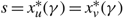 \[s=x_{u}^{*}(\gamma )=x_{v}^{*}(\gamma )\]
satisfy the conditions of Lemma 8.
\[s=x_{u}^{*}(\gamma )=x_{v}^{*}(\gamma )\]
satisfy the conditions of Lemma 8.
Let γ = min{γu, γv}, and consider the case in which γ = γu ≤ γv. The arguments for the case in which γ = γ v < γu are analogous.
When γ = γu ≤ γv, we have, by Corollary 3, αu ≤ Ωu = Ω(γ), gx(x, u γ) > 0 for αu < x < Ωu, and if 0 < αu then gx(x, u, γ) < 0 for x < αu. Furthermore, since γ = γu = γ u (αu, Ωu), g(αu, u, γ) = –U. Finally, if h ≥ 0, then α(γ) = αu = 0 and if h < 0 then α(γ) = max{0 (γ + (U – p)v)/h ≤ max {0 (γ + (U – p)u)/h} = αu. Let Ω = Ωu = Ω(γ), and consider the two cases α(γ) = αu and α(γ) < αu.
Case 1: α(γ) = αu. In this case let α = αu α(γ), and observe that g(α, v, γ) = g(α, u, γ) = –U and, by Lemma 7,
 \[\frac{{{\sigma }^{2}}}{2}({{g}_{x}}(\alpha ,v,\gamma )-{{g}_{x}}(\alpha ,u,\gamma ))=(v-u)(U-p)>0.\]
Furthermore, by Lemma 6, g(Ω, v, γ) ≤ M = g(Ω, u, γ). Thus, there is a point S ∈ (α, Ω] such that g(S, u, γ) = g(S, v, γ), g(x, v, γ) = g(x, u, γ) for α < x < S, and gx(S, v, γ) ≤ gx(S, u, γ).
If gx(S, u, γ) = gx(S, v, γ) then, by Lemma 4, g(S, u, γ) = –p and, by Corollary 3, gx(x, u, γ) > 0 for S ≤ x < Ω
u
, so
 \[S=x_{u}^{*}(\gamma )\]
. Since gx(α, v, γ) > gx(α, u, γ) > 0 and gx(S, v, γ) = gx(S, v, γ) gx(S, u, γ), and gx(x, μ, γ) is either convex or concave by Lemma 5, gx(x, v, γ) > 0 for α ≤ x ≤ S, and so
\[S=x_{u}^{*}(\gamma )\]
. Since gx(α, v, γ) > gx(α, u, γ) > 0 and gx(S, v, γ) = gx(S, v, γ) gx(S, u, γ), and gx(x, μ, γ) is either convex or concave by Lemma 5, gx(x, v, γ) > 0 for α ≤ x ≤ S, and so
 \[S=x_{v}^{*}(\gamma )\]
as well. But then S and γ satisfy the conditions of Lemma 8.
\[S=x_{v}^{*}(\gamma )\]
as well. But then S and γ satisfy the conditions of Lemma 8.
If gx(S, u, γ) > gx(S, v, γ) then, again by Lemma 7, gx(S, u, γ) > –p and, since gx(x, u, γ) > 0 for α < x < Ω, we see that
 \[\alpha \lt x_{u}^{*}(\gamma ) \lt S\]
and
\[\alpha \lt x_{u}^{*}(\gamma ) \lt S\]
and
 \[g(x_{u}^{*}(\gamma ),v,\gamma )>g(x_{u}^{*}(\gamma ),u,\gamma )=-p\]
, from which it follows that
\[g(x_{u}^{*}(\gamma ),v,\gamma )>g(x_{u}^{*}(\gamma ),u,\gamma )=-p\]
, from which it follows that
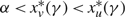 \[\alpha \lt x_{v}^{*}(\gamma ) \lt x_{u}^{*}(\gamma )\]
.
\[\alpha \lt x_{v}^{*}(\gamma ) \lt x_{u}^{*}(\gamma )\]
.
Case 2: α (γ) < α u. In this case, h < 0 and we argue that gx(x, v, γ) is positive for x > α(γ). To see this, observe that either α (γ) = 0 > (γ + U – p) v)/h, in which case
 \[{{C}_{v}}(\gamma )=-\frac{h}{v}(\frac{\gamma +(U-p)v}{h}+\frac{{{\sigma }^{2}}}{2v}),\]
and so
 \[{{g}_{x}}(x,v,\gamma )=-h(\frac{1-{{\text{e}}^{-2vx/{{\sigma }^{2}}}}}{v}-{{\text{e}}^{-2vx/{{\sigma }^{2}}}}\frac{2}{{{\sigma }^{2}}}\frac{\gamma +(U-p)v}{h}),\]
which is positive for all x ≥ 0, or α(γ) = (γ + U – p)v)/h ≥ 0, in which case
 \[{{C}_{v}}(\gamma )=-\frac{h}{v}{{\text{e}}^{2v\alpha (\gamma )/{{\sigma }^{2}}}}(\frac{\gamma +(U-p)v}{h}+\frac{{{\sigma }^{2}}}{2v}-\alpha (\gamma ))=-\frac{h{{\sigma }^{2}}}{2{{v}^{2}}}{{\text{e}}^{2v\alpha (\gamma )/{{\sigma }^{2}}}},\]
and so
 \[{{g}_{x}}(x,v,\gamma )=-\frac{h}{v}(1-{{\text{e}}^{-2v(x-\alpha (\gamma ))/{{\sigma }^{2}}}}),\]
which is positive for all x > α (γ).
Since g(α(γ), v, γ) = g(α(u), u, γ) = –U and g(⋅, v, γ) is increasing and, by Corollary 3, g(⋅, u, γ) is decreasing on (α(γ), αu), there must be a unique point s ∈ (α(γ), αu) such that g(s, v, γ) = g(s, u, γ) and, by Lemma 7, g(s, v, γ) < –p. Furthermore, by Lemma 6, g(Ω, v, γ) ≤ M = g(Ω, u, γ), and so there must be a point S ∈ (αu, Ω) such that g(S, v, γ) = g(S, u, γ), g(x, v, γ) > g(x, u, γ) for s < x < S and gx(S, v, γ) ≤ gx(S, u, γ).
If gx(S, v, γ) = gx(S, v, γ) then, by Lemma 7, g(S, v, γ) = –p, and so S and γ satisfy the conditions of Lemma 8.
If gx(S, v, γ) < gx(S, u, γ) then, by Lemma 7, g(S, v, γ) > –p. Since g(s, u, γ) = g(s, v, γ) < –p, g(x,v,y) > g(x,u,y) for s < x < S and g(s,v,y) = g(S,u,γ) > –p, it follows that
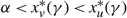 $x_v^*(\gamma ) \lt x_u^*(\gamma )$
.
$x_v^*(\gamma ) \lt x_u^*(\gamma )$
.
We now argue that, as γ reaches the lower bound in (34),
 $x_u^*(\gamma ) \le x_v^*(\gamma )$
.
$x_u^*(\gamma ) \le x_v^*(\gamma )$
.
Case (a): h = 0. We consider the case in which u < v < 0. The arguments for the other cases are analogous. In this case, min{0,–(U–p)v (M + p)u} = –(U–p)v > (M + p)u and
 $$\mathop {\lim }\limits_{\gamma \to - (U - p)v} x_v^*(\gamma ) = {{{\sigma ^2}} \over {2v}}\mathop {\lim }\limits_{\gamma \to - (U - p)v} \log [{{\gamma + (U - p)v} \over \gamma }] = \infty ,$$
while
 $$\mathop {\lim }\limits_{\gamma \to - (U - p)v} x_u^*(\gamma ) = \Theta + {{{\sigma ^2}} \over {2u}}\log [1 + {{(M + p)u} \over {(U - p)v}}] \lt \Theta .$$
Case (b): h > 0. In this case the lower bound in (34) is
 $$\gamma = - (U - p)v - {{h{\sigma ^2}} \over {2v}}(1 + {W_{k(vh)}}[ - {{\rm{e}}^{ - 1 - 2(U - p){v^2}/h{\sigma ^2}}}]),$$
and we see from (43) that w(v,γ) = –1, and so
 $x_v^*(\gamma ) = \gamma /h$
. In this case α = 0 and Ω(γ) = min{Θ (γ – (M + p)u)/h} = (γ – (M + p)u)/h – ε for some ε ≥ 0, and so, if u > 0,
$x_v^*(\gamma ) = \gamma /h$
. In this case α = 0 and Ω(γ) = min{Θ (γ – (M + p)u)/h} = (γ – (M + p)u)/h – ε for some ε ≥ 0, and so, if u > 0,
 $$w(u,\gamma ) = {W_{ - 1}}[{{\rm{e}}^{ - 2(M + p){u^2}/h{\sigma ^2}}}{{\rm{e}}^{ - 1 - 2u\varepsilon /{\sigma ^2}}}( - 1 - {{2u} \over {{\sigma ^2}}}\varepsilon )] \lt - 1 - {{2u} \over {{\sigma ^2}}}\varepsilon ,$$
where the last inequality follows from the fact that W –1 is a decreasing function, and
 $$x_u^*(\gamma ) = {\gamma \over h} + {{{\sigma ^2}} \over {2u}}(1 + w(u,\gamma )) \lt {\gamma \over h} - \varepsilon \le x_v^*(\gamma ).$$
If u < 0,
 $$w(u,\gamma ) = {W_0}[{{\rm{e}}^{ - 2(M + p){u^2}/h{\sigma ^2}}}{{\rm{e}}^{ - 1 - 2u\varepsilon /{\sigma ^2}}}( - 1 - {{2u} \over {{\sigma ^2}}}\varepsilon )],$$
and either –1–2uε/σ 2 ≥ 0, in which case w(u,γ) ≥ 0 and
 $$x_u^*(\gamma ) \lt \gamma /h = x_v^*(\gamma ),$$
or –1–2uɛ/σ 2 < 0, in which case, since W 0 is an increasing function, w(u,γ) > –1 –2uɛ/σ 2 and
$$x_u^*(\gamma ) \lt \gamma /h = x_v^*(\gamma ),$$
or –1–2uɛ/σ 2 < 0, in which case, since W 0 is an increasing function, w(u,γ) > –1 –2uɛ/σ 2 and
 $$x_u^*(\gamma ) = {\gamma \over h} + {{{\sigma ^2}} \over {2u}}(1 + w(u,\gamma )) < {\gamma \over h} - \varepsilon \le x_v^*(\gamma ).$$
The arguments for the h < 0 case are analogous.
In Figure 1 we illustrate an optimal policy and the associated functions g(·, u, γ) and g(·, v, γ) for a case in which h > 0, Θ is finite, and K = 0.
Figure 1. Optimal values for s, γ, α(γ), and Ω(γ), and the associated functions g(·, u, γ) (thin line) and g(·, v, γ) (thick line) for a problem with two drift rates where h > 0, Θ is finite, and K = 0. To explore other cases, download a Wolfram computable document format application from https://www2.isye.gatech.edu/faculty/John_VandeVate/EconomicAvgCost.html.
Let
 $\underline \gamma $
denote the the optimal average cost for the economic average cost Brownian control problem when K = 0.
$\underline \gamma $
denote the the optimal average cost for the economic average cost Brownian control problem when K = 0.
Corollary 6
 $$\eqalign{\alpha (\gamma ) & \lt x_v^*(\gamma ) \lt x_u^*(\gamma ) \lt \Omega (\gamma ), \cr g(x_v^*(\gamma ),u,\gamma ) & \lt - p\quad { and}\quad g(x_u^*(\gamma ),v,\gamma ) \gt - p } $$
for
 $\underline \gamma \lt \gamma \le \min \{ {\gamma _u},{\gamma _v}\} $
.
$\underline \gamma \lt \gamma \le \min \{ {\gamma _u},{\gamma _v}\} $
.
In Corollary 7 we provide a closed-form expression for the average cost and parameters defining an optimal policy when h > 0 and the upper limit on the buffer capacity is not constraining. Its proof is given in Appendix C.
Corollary 7
Under Assumption 3, when h > 0, let
 $$\eqalign{ w & = {W_{k(u)}}[ - {{\rm{e}}^{ - 1 - 2(M + p){u^2}/h{\sigma ^2}}}], \cr s = & \underline \gamma {1 \over h} + {{{\sigma ^2}} \over {2u}}(w + 1), \cr \underline \gamma & = - (U - p)v - {{h{\sigma ^2}} \over {2v}}\left(1 + {W_{k(v)}}({{\rm{e}}^{ - 1 - 2(U - p){v^2}/h{\sigma ^2} + v(w + 1)/u}}({v \over u}(w + 1) - 1))\right),} $$
where k(μ) = 0 if μ < 0 and –1 otherwise. If
 $$\underline \gamma \le h\Theta + (M + p)u$$
then
$$\underline \gamma \le h\Theta + (M + p)u$$
then
 $\underline \gamma $
and s satisfy the conditions of Lemma 8, proving that
$\underline \gamma $
and s satisfy the conditions of Lemma 8, proving that
 $\Phi = \{ (u,s,v,\Omega (\underline \gamma ),u),(v,0,v,s,u)\} $
is an optimal policy and
$\Phi = \{ (u,s,v,\Omega (\underline \gamma ),u),(v,0,v,s,u)\} $
is an optimal policy and
 ${\rm{AC}}(\Phi ) = \underline \gamma $
.
${\rm{AC}}(\Phi ) = \underline \gamma $
.
Corollary 8 extends Lemma 10 to the problem with more than two drift rates.
4.2 When K > 0
In Section 4.1 we addressed the problem in which the cost K to change the drift rate is 0. In this section we address the problem when K > 0. Note that
 $\overline \gamma = \min \{ {\gamma _u},{\gamma _v}\} $
provides an upper bound and
$\overline \gamma = \min \{ {\gamma _u},{\gamma _v}\} $
provides an upper bound and
 $\underline \gamma $
provides a lower bound on the average cost of a policy in this case. In Lemma 11 we show how, given an average cost γ between these bounds, to construct functions δ and a policy Φ(γ) that satisfy (23)–(25) and (27)–(29), and so prove that Φ(γ) is an optimal policy when
$\underline \gamma $
provides a lower bound on the average cost of a policy in this case. In Lemma 11 we show how, given an average cost γ between these bounds, to construct functions δ and a policy Φ(γ) that satisfy (23)–(25) and (27)–(29), and so prove that Φ(γ) is an optimal policy when
 $K = \Delta (\gamma ) \equiv \int_0^\Theta (\delta (x,v,\gamma ) - \delta (x,u,\gamma )) {\rm{d}}x$
. In Lemma 12 we argue that Δ(·) is a continuous, increasing function on
$K = \Delta (\gamma ) \equiv \int_0^\Theta (\delta (x,v,\gamma ) - \delta (x,u,\gamma )) {\rm{d}}x$
. In Lemma 12 we argue that Δ(·) is a continuous, increasing function on
 $ (\underline \gamma ,\overline \gamma ) $
and so conclude that, for
$ (\underline \gamma ,\overline \gamma ) $
and so conclude that, for
 $0 \lt K \lt \Delta (\overline \gamma )$
, we can use binary search to find the value
$0 \lt K \lt \Delta (\overline \gamma )$
, we can use binary search to find the value
 $\underline \gamma < \gamma < \overline \gamma$
such that Δ(γ) = K and so Φ(γ) is an optimal policy.
$\underline \gamma < \gamma < \overline \gamma$
such that Δ(γ) = K and so Φ(γ) is an optimal policy.
Lemma 11
Under Assumptions 2 and 3, given
 $\overline \gamma \ge \gamma \gt \underline \gamma ,$
let
$\overline \gamma \ge \gamma \gt \underline \gamma ,$
let
 $$\eqalign{ & \alpha (\gamma ) = \left\{ {\matrix{ {\max \{ 0,{{\gamma + (U - p)v} \over h}\} } & { \;if\; h \lt 0,} \cr 0 & { \;if\; h \ge 0,} \cr } } \right. \cr & \Omega (\gamma ) = \left\{ {\matrix{ {\min \{ \Theta ,{{\gamma - (M + p)u} \over h}\} } & { \;if\; h \gt 0,} \cr \Theta & { \;if\; h \le 0,} } } \right.} $$
where Cu(γ) is determined by g(Ω(γ), u, γ) = M and Cv(γ) is determined by g(α(γ), v, γ) = –U. Then there exists a unique point
 $$s(\gamma ) \in [\alpha (\gamma ),x_v^*(\gamma ))$$
such that g(s, u, γ) = g(s, v,γ) and a unique point
$$s(\gamma ) \in [\alpha (\gamma ),x_v^*(\gamma ))$$
such that g(s, u, γ) = g(s, v,γ) and a unique point
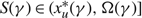 $S(\gamma ) \in (x_u^*(\gamma ),\Omega (\gamma )]$
such that g(S, u, γ) = g(S, v,γ) and γ and the functions
$S(\gamma ) \in (x_u^*(\gamma ),\Omega (\gamma )]$
such that g(S, u, γ) = g(S, v,γ) and γ and the functions
 $$\delta (x,u,\gamma ) = \left\{ {\matrix{ { - U,} & {0 \le x \lt \alpha (\gamma ),} \cr {g(x,v,\gamma ),} & {\alpha (\gamma ) \le x \lt s(\gamma ),} \cr {g(x,u,\gamma ),} & {s(\gamma ) \le x \lt \Omega (\gamma ),} \cr {M,} & {\Omega (\gamma ) \lt x \le \Theta ,} \cr } } \right.$$
and
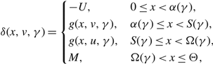 $$\delta (x,v,\gamma ) = \left\{ {\matrix{ { - U,} & {0 \le x \lt \alpha (\gamma ),} \cr {g(x,v,\gamma ),} & {\alpha (\gamma ) \le x \lt S(\gamma ),} \cr {g(x,u,\gamma ),} & {S(\gamma ) \le x \lt \Omega (\gamma ),} \cr {M,} & {\Omega (\gamma ) \lt x \le \Theta ,} \cr } } \right.$$
satisfy (23)–(25) and (27)–(29) with respect to the policy Φ( γ) = {(u, s(γ), v, Ω(γ), u) (v, α(γ), v, S(γ), u)}, proving that Φ(γ) is an optimal policy for the problem with changeover cost
 $K = \Delta (\gamma ) = \int_0^\Theta \left( {\delta (x,v,\gamma ) - \delta (x,u,\gamma )} \right) {\rm{d}}x$
.
$K = \Delta (\gamma ) = \int_0^\Theta \left( {\delta (x,v,\gamma ) - \delta (x,u,\gamma )} \right) {\rm{d}}x$
.
Proof. We first argue that there is a point
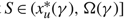 $$S \in (x_u^*(\gamma ),\Omega (\gamma )]$$
such that g(S, v, γ) = g(S, u, γ). To see this, observe that, by Corollary 6,
$$S \in (x_u^*(\gamma ),\Omega (\gamma )]$$
such that g(S, v, γ) = g(S, u, γ). To see this, observe that, by Corollary 6,
 $g(x_u^*(\gamma ),v,\gamma ) \gt g(x_u^*(\gamma ),u,\gamma ) = - p$
and, by Lemma 6, g(Ω(γ), v, γ) ≤ g(Ω(γ), u, γ) = M. Thus, there is a point
$g(x_u^*(\gamma ),v,\gamma ) \gt g(x_u^*(\gamma ),u,\gamma ) = - p$
and, by Lemma 6, g(Ω(γ), v, γ) ≤ g(Ω(γ), u, γ) = M. Thus, there is a point
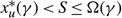 $x_u^*(\gamma ) \lt S \le \Omega (\gamma )$
such that g(S, v, γ) = g(S, u, γ). Similarly, since
$x_u^*(\gamma ) \lt S \le \Omega (\gamma )$
such that g(S, v, γ) = g(S, u, γ). Similarly, since
 $g(x_v^*(\gamma ),u,\gamma ) \lt g(x_v^*(\gamma ),v,\gamma ) = - p$
, by Corollary 6 and g(α(γ), u, γ) ≥ g(α(γ), u, γ) = –U by Lemma 6, there is a point
$g(x_v^*(\gamma ),u,\gamma ) \lt g(x_v^*(\gamma ),v,\gamma ) = - p$
, by Corollary 6 and g(α(γ), u, γ) ≥ g(α(γ), u, γ) = –U by Lemma 6, there is a point
 $\alpha (\gamma ) \le s \lt x_v^*(\gamma )$
such that g(s, v, γ) = g(s, u, γ).
$\alpha (\gamma ) \le s \lt x_v^*(\gamma )$
such that g(s, v, γ) = g(s, u, γ).
We next observe that, since g(·, u, γ) is increasing on
 $[x_u^*(\gamma ),\Omega (\gamma ))$
by Lemma 9, g(S, u, γ) > –p and so, by Lemma 7, gx(S, v, γ) < g
x
(S, u, γ). Similarly, since g(·, v, γ) is increasing in
$[x_u^*(\gamma ),\Omega (\gamma ))$
by Lemma 9, g(S, u, γ) > –p and so, by Lemma 7, gx(S, v, γ) < g
x
(S, u, γ). Similarly, since g(·, v, γ) is increasing in
 $$(\alpha (\gamma ),x_v^*(\gamma )]$$
by Lemma 9, g(s, v, γ) < –p and so, by Lemma 7, gx(s, v, γ) > gx(s, v, γ).
$$(\alpha (\gamma ),x_v^*(\gamma )]$$
by Lemma 9, g(s, v, γ) < –p and so, by Lemma 7, gx(s, v, γ) > gx(s, v, γ).
To see that s and S are unique, suppose that there are roots S < S
1 < S
2 < … ≤ Ω(γ) and s > s
1 > s
2 > … ≥ α(γ) of g(·, v, γ) – g(·, u, γ). Since gx(S, v, γ) < gx(S, u, γ), we must have gx(S
1, v, γ) ≥ gx(S
1, u, γ) and so, by Lemma 7, g(S
1, u γ) ≤ –p, which contradicts the fact that g(·, u, γ) is increasing on
 $[x_u^*(\gamma ),\Omega (\gamma ))$
. Similarly, since gx(x, v, γ) > gx(s, u, γ), we must have gx(s
1, v, γ) ≤ gx(s
1, u, γ) and so, by Lemma 7, g(s
1, v, γ) ≥ –p, which contradicts the fact the g(·, v, γ) is increasing on
$[x_u^*(\gamma ),\Omega (\gamma ))$
. Similarly, since gx(x, v, γ) > gx(s, u, γ), we must have gx(s
1, v, γ) ≤ gx(s
1, u, γ) and so, by Lemma 7, g(s
1, v, γ) ≥ –p, which contradicts the fact the g(·, v, γ) is increasing on
 $ (\alpha (\gamma ),x_v^*(\gamma )] $
.
$ (\alpha (\gamma ),x_v^*(\gamma )] $
.
We next argue that the functions δ satisfy (25). The functions g(·, u, γ) and g(·, v, γ) satisfy (25) with equality for all real x. Since g(·, v, γ) is increasing on
 $ (\alpha (\gamma ),x_v^*(\gamma )] $
, the fact that
$ (\alpha (\gamma ),x_v^*(\gamma )] $
, the fact that
 $\alpha (\gamma ) \le s < x_v^*(\gamma )$
ensures that g(x, v, γ) < –p for all x ∈ [α(γ), s] and so, by Lemma 7, δ(x, u, γ) satisfies (25) for x ∈ [α(γ), s]. Similarly, we see that g(·, u, γ) > –p for x ∈ [S, Ω(γ)] and so δ(x, v, γ) satisfies (25) for x ∈ [S, Ω(γ)]. If Ω(γ) < Θ then h > 0, Ω(γ) = (γ –(M + p)u)/h < Θ, and
$\alpha (\gamma ) \le s < x_v^*(\gamma )$
ensures that g(x, v, γ) < –p for all x ∈ [α(γ), s] and so, by Lemma 7, δ(x, u, γ) satisfies (25) for x ∈ [α(γ), s]. Similarly, we see that g(·, u, γ) > –p for x ∈ [S, Ω(γ)] and so δ(x, v, γ) satisfies (25) for x ∈ [S, Ω(γ)]. If Ω(γ) < Θ then h > 0, Ω(γ) = (γ –(M + p)u)/h < Θ, and
 $${{{\sigma ^2}} \over 2}{\delta _x}(x,\mu ,\gamma ) + \mu \delta (x,\mu ,\gamma ) + p\mu + hx = \mu (M + p) + hx \ge u(M + p) + h\Omega (\gamma ) = \gamma ,$$
proving that δ satisfies (25) on (Ω)(γ), Θ]. Similarly, if α (γ) > 0 then h < 0, α (γ) = (γ + (U – p)v)/h , and
 $${{{\sigma ^2}} \over 2}{\delta _x}(x,\mu ,\gamma ) + \mu \delta (x,\mu ,\gamma ) + p\mu + hx = \mu (M + p) + hx \ge u(M + p) + h\Omega (\gamma ) = \gamma ,$$
proving that δ satisfies (25) on [0, α (γ)).
The facts that s and S are roots of g(·, v, γ) – g(·, u, γ), g(α(γ), v, γ) = – U, and g(Ω(γ), u, γ) = M ensure that δ(·, μ, γ) is continuous for each μ ∈ {u, v} and satisfies (24).
To see that δ satisfies (23), observe that the choices of s(γ) and S(γ)ensure that δ(x, v, γ) ≥ δ(x, u, γ) for all
 $x \in {\cal R}$
.
$x \in {\cal R}$
.
Note that, by Lemma 6, g(x, v, γ) ≤ M and g(x, u, γ) ≥ –U for all x ∈ (α(γ), Ω(γ)). The facts that g(α(γ), v, γ) = –U, g(x, v, γ) is increasing on
 $ (\alpha (\gamma ),x_v^*(\gamma )],$
and g(x, v, γ) ≥ g(x, u, γ)
on (s(γ), S(γ)) ensure that g(x, v, γ) ≥ –U
for x ∈ [α(γ), S(γ)]. Similarly, the facts that g(Ω(γ), u, γ) = M, g(⋅, u, γ) is increasing in
$ (\alpha (\gamma ),x_v^*(\gamma )],$
and g(x, v, γ) ≥ g(x, u, γ)
on (s(γ), S(γ)) ensure that g(x, v, γ) ≥ –U
for x ∈ [α(γ), S(γ)]. Similarly, the facts that g(Ω(γ), u, γ) = M, g(⋅, u, γ) is increasing in
 $[x_u^*(\gamma ),\Omega (\gamma )],$
and g(x, u, γ) ≤ g(x, v, γ) for x ∈ (s(γ), S(γ)) ensure that g(x, u, γ) ≤ M for x ∈ [s(γ), Ω(γ)].
$[x_u^*(\gamma ),\Omega (\gamma )],$
and g(x, u, γ) ≤ g(x, v, γ) for x ∈ (s(γ), S(γ)) ensure that g(x, u, γ) ≤ M for x ∈ [s(γ), Ω(γ)].
Finally, by assumption, K = Δ(γ) and so δ and γ satisfy (22). Thus, we conclude that δ, γ, and Φ(γ) satisfy all the conditions of Proposition 3 and Corollary 4, proving that γ is a lower bound on the cost of any nonanticipating policy and, since AC(Φ(γ)) = γ, Φ(γ) is an optimal policy.
In Figure 2 we illustrate the policy and the functions
 $g( \cdot ,u,\overline \gamma )$
and
$g( \cdot ,u,\overline \gamma )$
and
 $g( \cdot ,v,\overline \gamma )$
constructed in Lemma 11 for a case in which h > 0, Θ is finite,
$g( \cdot ,v,\overline \gamma )$
constructed in Lemma 11 for a case in which h > 0, Θ is finite,
 $$\overline \gamma = {\gamma _v} \lt {\gamma _u},$$
and
$$\overline \gamma = {\gamma _v} \lt {\gamma _u},$$
and
 $K = \overline K $
.
$K = \overline K $
.

Figure 2. The policy and the functions
 $g( \cdot ,u,\overline \gamma )$
and
$g( \cdot ,u,\overline \gamma )$
and
 $g( \cdot ,v,\overline \gamma )$
constructed in Lemma 11 for a case in which h > 0, Θ is finite,
$g( \cdot ,v,\overline \gamma )$
constructed in Lemma 11 for a case in which h > 0, Θ is finite,
 $\overline \gamma = {\gamma _v} \lt {\gamma _u},$
and
$\overline \gamma = {\gamma _v} \lt {\gamma _u},$
and
 $K = \overline K $
. Here
$K = \overline K $
. Here
 $\Delta (\overline \gamma )$
is the highlighted area between
$\Delta (\overline \gamma )$
is the highlighted area between
 $g( \cdot ,v,\overline \gamma )$
and
$g( \cdot ,v,\overline \gamma )$
and
 $g( \cdot ,u,\overline \gamma )$
. To explore other cases, download a Wolfram computable document format application from https://www2.isye.gatech.edu/faculty/John_VandeVate/EconomicAvgCost.html.
$g( \cdot ,u,\overline \gamma )$
. To explore other cases, download a Wolfram computable document format application from https://www2.isye.gatech.edu/faculty/John_VandeVate/EconomicAvgCost.html.
Corollary 9
 $K \gt \overline K \equiv \Delta (\overline \gamma ) = \int_0^\Theta (\delta (x,v,\overline \gamma ) - \delta (x,u,\overline \gamma )) {\rm{d}}x,$
where δ is defined by (37) and (38), then
 $$\overline \gamma $$
is a lower bound on the average cost of a policy and the better of the two single-rate policies is an optimal policy.
$$\overline \gamma $$
is a lower bound on the average cost of a policy and the better of the two single-rate policies is an optimal policy.
Observe that Δ(⋅) is a continuous function of γ with
 $\Delta (\overline \gamma ) = \overline K $
and
$\Delta (\overline \gamma ) = \overline K $
and
 $\Delta (\underline \gamma ) = 0$
. Thus, for each
$\Delta (\underline \gamma ) = 0$
. Thus, for each
 $\overline K \gt K \gt 0,$
there exists
$\overline K \gt K \gt 0,$
there exists
 $\overline \gamma \gt \gamma \gt \underline \gamma $
such that Δ(γ) = K, and so γ, δ(⋅, μ, γ) for μ
∈ {u, v}, and Φ(γ) satisfy (22)–(29), proving that γ is a lower bound on the average cost of a policy and, since AC(Φ(γ)) = γ, Φ(γ) is an optimal policy. In Lemma 12 we show that Δ is increasing and so we can find γ using binary search.
$\overline \gamma \gt \gamma \gt \underline \gamma $
such that Δ(γ) = K, and so γ, δ(⋅, μ, γ) for μ
∈ {u, v}, and Φ(γ) satisfy (22)–(29), proving that γ is a lower bound on the average cost of a policy and, since AC(Φ(γ)) = γ, Φ(γ) is an optimal policy. In Lemma 12 we show that Δ is increasing and so we can find γ using binary search.
Lemma 12
The function
 $$\Delta (\gamma ) = \int_0^\Theta (\delta (x,v,\gamma ) - \delta (x,u,\gamma )) {\rm{d}}x,$$
where δ is defined by (37) and (38), is continuous and increasing on
 $ (\underline \gamma ,\overline \gamma ) $
.
$ (\underline \gamma ,\overline \gamma ) $
.
Proof. Since g(s(γ), u, γ)) = g(s(γ), v, γ) and g(S(γ), u, γ) = g(S(γ), v, γ),
 $$\eqalign{{\Delta ^{'}}(\gamma ) & = \int_{s(\gamma )}^{S(\gamma )} ({\partial _\gamma }g(x,v,\gamma ) - {\partial _\gamma }g(x,u,\gamma )) {\rm{d}}x \cr & = \int_{s(\gamma )}^{S(\gamma )} ({1 \over v} + {{\rm{e}}^{ - 2vx/{\sigma ^2}}}C_v^{'}(\gamma ) - {1 \over u} - {{\rm{e}}^{ - 2ux/{\sigma ^2}}}C_u^{'}(\gamma )) {\rm{d}}x \cr & = \int_{s(\gamma )}^{S(\gamma )} ({1 \over v}(1 - {{\rm{e}}^{2v(\alpha (\gamma ) - x)/{\sigma ^2}}}(1 + {{2v} \over {{\sigma ^2}}}(\gamma + (U - p)v - h\alpha (\gamma )){\alpha ^{'}}(\gamma ))) \cr & \quad - {1 \over u}(1 - {{\rm{e}}^{2u(\Omega (\gamma ) - x)/{\sigma ^2}}}(1 + {{2u} \over {{\sigma ^2}}}(\gamma - (M + p)u - h\Omega (\gamma )){\Omega ^{'}}(\gamma )))) {\rm{d}}x,} $$
where
 $$\eqalign{{\alpha ^{'}}(\gamma ) & = \left\{ {\matrix{ 0 & {{\rm{if}}\;h \ge 0\;{\rm{or}}(\gamma + (U - p)v)/h \lt 0,} \cr {{1 \over h}} & {{\rm{if}}\;h \lt 0\;{\rm{and}}(\gamma + (U - p)v)/h \ge 0,} \cr } } \right. \cr & {\Omega ^{'}}(\gamma ) = \left\{ {\matrix{ 0 & {{\rm{if}}\;h \le 0\;{\rm{or}}(\gamma - (M + p)u)/h \gt \Theta ,} \cr {{1 \over h}} & {{\rm{if}}\;h \gt 0\;{\rm{and}}(\gamma - (M + p)u)/h \le \Theta ,} \cr } } \right. \cr} $$
and so
 $${\Delta ^{'}}(\gamma ) = \int_{s(\gamma )}^{S(\gamma )} ({1 \over v}(1 - {{\rm{e}}^{2v(\alpha (\gamma ) - x)/{\sigma ^2}}}) - {1 \over u}(1 - {{\rm{e}}^{2u(\Omega (\gamma ) - x)/{\sigma ^2}}})) {\rm{d}}x \gt 0$$
so long as s(γ) < S(γ), i.e. so long as
 $\gamma \gt \underline \gamma $
. □
$\gamma \gt \underline \gamma $
. □
5. Conclusion
In this paper we extended a classical problem of controlling a Brownian motion by allowing the controller to employ instantaneous controls at any time. We characterized the conditions under which the resulting economic average cost Brownian control problem admits an optimal policy and showed that, when it does, a control band policy is optimal. We developed a simple method to calculate optimal policy parameters, namely economic bounds on the buffer and bands within which each drift rate should be used. This type of policy is straightforward to understand and implement, and could provide significant savings over ad-hoc methods. Furthermore, we provided explicit formulae for critical performance metrics, such as the frequencies with which the drift rate changes, work is rejected, and capacity is idled, for any control band policy, thereby helping the controller to better evaluate the impact of a chosen policy.
Our approach provides a clean and analytical solution which lends itself to further generalizations in terms of the form of the cost function. A future direction worth pursuing is to extend the method to handle the cases with more than two available rates.
Appendix A. Proof of the lemmas
Proof of Lemma 3. We present the proof for the h > 0 case, the argument for h < 0 is analogous. Note that z is a solution to (15) if and only if
 $$ - 1 - {{2(M + U){\mu ^2}} \over {h{\sigma ^2}}} = {{2\mu } \over {{\sigma ^2}}}z - {{\rm{e}}^{2\mu z/{\sigma ^2}}}.$$
By Assumption 1, the left-hand side of (39) is less than or equal to –1. The right-hand side is a decreasing function of z that is equal to –1 when z = 0 and goes to –∞ as z goes to ∞. Thus, there exists a unique nonnegative solution Ω*(μ) to (15).
To see that (16) characterizes this solution, observe that (39) can be written as –1–2(M + U)μ
2/hσ
2 = log(–w) + w, where w
= –e2μz/σ 2, and so w must be a solution to
 $w{{\rm{e}}^w} = - {{\rm{e}}^{ - 1 - 2(M + U){\mu ^2}/h{\sigma ^2}}}$
. Finally, observe that, since
$w{{\rm{e}}^w} = - {{\rm{e}}^{ - 1 - 2(M + U){\mu ^2}/h{\sigma ^2}}}$
. Finally, observe that, since
 $ - {{\rm{e}}^{ - 1}} \le - {{\rm{e}}^{ - 1 - 2(M + U){\mu ^2}/h{\sigma ^2}}} \lt 0,$
the system
$ - {{\rm{e}}^{ - 1}} \le - {{\rm{e}}^{ - 1 - 2(M + U){\mu ^2}/h{\sigma ^2}}} \lt 0,$
the system
 $w{{\rm{e}}^w} = - {{\rm{e}}^{ - 1 - 2(M + U){\mu ^2}/h{\sigma ^2}}}$
admits the real solutions
$w{{\rm{e}}^w} = - {{\rm{e}}^{ - 1 - 2(M + U){\mu ^2}/h{\sigma ^2}}}$
admits the real solutions
 ${w_{ - 1}} = {W_{ - 1}}( - {{\rm{e}}^{ - 1 - 2(M + U){\mu ^2}/h{\sigma ^2}}}) \le - 1$
and
${w_{ - 1}} = {W_{ - 1}}( - {{\rm{e}}^{ - 1 - 2(M + U){\mu ^2}/h{\sigma ^2}}}) \le - 1$
and
 ${w_0} = {W_0}( - {e^{ - 1 - 2(M + U){\mu ^2}/h{\sigma ^2}}}) \ge - 1$
. The fact that
${w_0} = {W_0}( - {e^{ - 1 - 2(M + U){\mu ^2}/h{\sigma ^2}}}) \ge - 1$
. The fact that
 $$\eqalign{{{2\mu } \over {{\sigma ^2}}}{\Omega ^*}(\mu ) & = - 1 - {{2(M + U){\mu ^2}} \over {h{\sigma ^2}}} - {W_k}( - {{\rm{e}}^{ - 1 - 2(M + U){\mu ^2}/h{\sigma ^2}}}) \cr & = \log [ - {w_k}{{\rm{e}}^{{w_k}}}] - {w_k} \cr & = \log [ - {w_k}]}$$
implies that either M + U = 0 and w –1 = w –0 = –1 and Ω*(μ) = 0 or only
 $$k = \left\{ {\matrix{{ - 1} & {{\rm{if}}\,\mu > 0} \cr 0 & {{\rm{if}}\,\mu < 0}\cr} } \right.$$
yields a positive value for Ω*(μ).
Proof of Lemma 5. Observe that
 $${g_x}(x,\mu ,\gamma ) = - {h \over \mu } - {{2\mu } \over {{\sigma ^2}}}{{\rm{e}}^{ - 2\mu x/{\sigma ^2}}}{C_\mu }(\gamma )\quad {\rm{and}}\quad {g_{x,x}}(x,\mu ,\gamma ) = {{4{\mu ^2}} \over {{\sigma ^4}}}{{\rm{e}}^{ - 2\mu x/{\sigma ^2}}}{C_\mu }(\gamma ).$$
Thus, we see that g(⋅, μ, γ) is convex if Cμ(γ) ≥ 0 and concave if Cμ(γ) ≤ 0. The unique root of gx(⋅, μ, γ) is (σ 2/2μ)log[–2μ 2 Cμ(γ)/σ 2 h], which is real only if Cμ(γ) and h have opposite signs. Finally, the fact that
 $${g_{x,x}}(x,v,\gamma ) - {g_{x,x}}(x,u,\gamma ) = {{4{v^2}} \over {{\sigma ^4}}}{{\rm{e}}^{ - 2vx/{\sigma ^2}}}{C_v}(\gamma ) - {{4{u^2}} \over {{\sigma ^4}}}{{\rm{e}}^{ - 2ux/{\sigma ^2}}}{C_u}(\gamma )$$
has the unique root x = (σ 2/2(v – u)) log[v 2 Cv (γ)/u Cu (γ)], which is only real if Cu (γ) and Cv (γ) have the same sign, implies gx(⋅, u, γ) – gx(⋅, v, γ) has at most two real roots.
Proof of Lemma 6. Consider a point
$x \in {\cal R}$
such that x > α. If
 $$\eqalign{M & \lt g(x,\mu ,\gamma ) \cr & = - p - {{hx} \over \mu } + {{h{\sigma ^2}} \over {2{\mu ^2}}} + {\gamma \over \mu } + {{\rm{e}}^{ - 2\mu x/{\sigma ^2}}}{C_\mu }(\gamma ) \cr & = - p - {{hx} \over \mu } + {{h{\sigma ^2}} \over {2{\mu ^2}}} + {\gamma \over \mu } + {{\rm{e}}^{ - 2\mu x/{\sigma ^2}}}{{\rm{e}}^{2\mu \alpha /{\sigma ^2}}}( - U + p - {{h{\sigma ^2}} \over {2{\mu ^2}}} - {\gamma \over \mu } + {{h\alpha } \over \mu }),} $$
then
 $$\eqalign{ & {\gamma \over \mu }({{\rm{e}}^{2\mu \alpha /{\sigma ^2}}} - {{\rm{e}}^{2\mu x/{\sigma ^2}}}) \cr & \quad \quad \lt {{\rm{e}}^{2\mu x/{\sigma ^2}}}( - M - p + {{h{\sigma ^2}} \over {2{\mu ^2}}} - {{hx} \over \mu }) + {{\rm{e}}^{2\mu \alpha /{\sigma ^2}}}( - U + p - {{h{\sigma ^2}} \over {2{\mu ^2}}} + {{h\alpha } \over \mu }). \cr} $$
Since
 $ ({{\rm{e}}^{2\mu \alpha /{\sigma ^2}}} - {{\rm{e}}^{2\mu x/{\sigma ^2}}})/\mu \lt 0 $
, this implies that
$ ({{\rm{e}}^{2\mu \alpha /{\sigma ^2}}} - {{\rm{e}}^{2\mu x/{\sigma ^2}}})/\mu \lt 0 $
, this implies that
 $$\gamma \gt {{{{\rm{e}}^{2\mu x/{\sigma ^2}}}(hx - h{\sigma ^2}/2\mu + \mu (M + p)) - {{\rm{e}}^{2\mu \alpha /{\sigma ^2}}} (h\alpha - h{\sigma ^2}/2\mu - \mu (U - p))} \over {{{\rm{e}}^{2\mu x/{\sigma ^2}}} - {{\rm{e}}^{2\mu \alpha /{\sigma ^2}}}}}.$$
But then, by (14), γ > γμ(α, x), the average cost of the control band policy (α, x) for the single drift rate μ, and so γμ ≤ γμ(α, x) < γ, contradicting our assumption that γ ≤ γμ.
When γ ≤ γμ and g(Ω, μ, γ) = M for some point
\[\Omega \in {\cal R}\]
, the proof that g(x, μ, γ) ≥ –U for all
$x \in {\cal R}$
such that x < Ω relies on similar arguments.
Proof of Lemma 7. Recall that g(⋅, μ, γ) satisfies (33), and so
 $$\eqalign{ & {{{\sigma ^2}} \over 2}{g_x}(x,v,\gamma ) + ug(x,v,\gamma ) + pu + hx - \gamma \cr & \quad \quad = {{{\sigma ^2}} \over 2}{g_x}(x,v,\gamma ) + ug(x,v,\gamma ) + pu + hx - {{{\sigma ^2}} \over 2}{g_x}(x,v,\gamma ) - vg(x,v,\gamma ) - pv - hx \cr & \quad \quad = (u - v)(g(x,v,\gamma ) + p). \cr} $$
If g(z, u, γ) = g(z, u, γ) for some point
\[z\in \mathbb R\]
then, since
 $${{{\sigma ^2}} \over 2}{g_x}(z,u,\gamma ) + ug(z,u,\gamma ) + pu + hz = \gamma = {{{\sigma ^2}} \over 2}{g_x}(z,v,\gamma ) + vg(z,v,\gamma ) + pv + hz,$$
we have
 $$(u - v)(g(z,v,\gamma ) + p) = {{{\sigma ^2}} \over 2}({g_x}(z,v,\gamma ) - {g_x}(z,u,\gamma )).$$
Proof of Lemma 9. We first consider the case h = 0. In this case α(γ) = 0, Ω(γ) = Θ, γ > max {0, –U – p)v (M + p)u}, and
 $${C_u}(\gamma ) = - {{\gamma - (M + p)u} \over u}{{\rm{e}}^{2u\Omega (\gamma )/{\sigma ^2}}}\quad {\rm and} \quad \quad \quad {C_v}(\gamma ) = - {{\gamma + (U - p)v} \over v}{{\rm{e}}^{2v\alpha (\gamma )/{\sigma ^2}}}.$$
Since
 $$g(x,\mu ,\gamma ) = - p + {\gamma \over \mu } + {{\rm{e}}^{ - 2\mu x/{\sigma ^2}}}{C_\mu }(\gamma ),$$
 $$x_\mu ^*(\gamma )$$
is the unique solution for z to g(z, μ, γ) = –p. Since γ > max {0 (M + p)u},
$$x_\mu ^*(\gamma )$$
is the unique solution for z to g(z, μ, γ) = –p. Since γ > max {0 (M + p)u},
 $$x_v^*(\gamma )$$
is real, and, since γ > max {0, –U –p)v},
$$x_v^*(\gamma )$$
is real, and, since γ > max {0, –U –p)v},
 $$x_v^*(\gamma )$$
is real.
$$x_v^*(\gamma )$$
is real.
To prove (35) and (36), observe that for μ ∈ {u, v},
$${g_x}(x,\mu ,\gamma ) = - {{2\mu } \over {{\sigma ^2}}}{{\rm{e}}^{ - 2\mu x/{\sigma ^2}}}{C_\mu }(\gamma ),$$
and so gx(x, u, γ) > 0 since γ > (M + p)u and gx(x, v, γ) > 0 since γ > (U + p)v.
We next consider the case in which h ≠ 0 and observe that, by Lemma 5, for each μ ∈ {u, v}, g(⋅, μ, γ) is either convex or concave, and so admits at most one point z satisfying g(z, μ, γ) = –p and gx(z, μ, γ) ≥ 0. To see that
 $$x_\mu ^*(\gamma )$$
satisfies
$$x_\mu ^*(\gamma )$$
satisfies
 $g(x_\mu ^*(\gamma ),\mu ,\gamma ) = - p$
, observe that, when h ≠ 0,
$g(x_\mu ^*(\gamma ),\mu ,\gamma ) = - p$
, observe that, when h ≠ 0,
 $$\eqalign{ & g(x_\mu ^*(\gamma ),\mu ,\gamma ) = - p + {{h{\sigma ^2}} \over {2{\mu ^2}}} - {h \over \mu }x_\mu ^*(\gamma ) + {\gamma \over \mu } + {{\rm{e}}^{ - 2\mu x_\mu ^*(\gamma )/{\sigma ^2}}}{C_\mu }(\gamma ) \cr & \,\,\,\,\,\,\,\,\,\,\,\,\,\,\,\,\,\,\,\,\,\,\,\,\,\,\,\,\,\, = - p + {{h{\sigma ^2}} \over {2{\mu ^2}}} - {h \over \mu }({\gamma \over h} + {{{\sigma ^2}} \over {2\mu }}(1 + w(\mu ,\gamma ))) + {\gamma \over \mu } \cr & \quad \,\,\,\,\,\,\,\,\,\,\,\,\,\,\,\,\,\,\,\,\,\,\, + {{\rm{e}}^{ - 2\mu (\gamma /h + {\sigma ^2}(1 + w(\mu ,\gamma ))/2\mu )/{\sigma ^2}}}{C_\mu }(\gamma ) \cr & \,\,\,\,\,\,\,\,\,\,\,\,\,\,\,\,\,\,\,\,\,\,\,\,\,\,\,\,\, = - p - {{\rm{e}}^{ - w(\mu ,\gamma )}}({{h{\sigma ^2}} \over {2{\mu ^2}}}w(\mu ,\gamma ){{\rm{e}}^{w(\mu ,\gamma )}} - {{\rm{e}}^{ - 2\mu (\gamma /h + {\sigma ^2}/2\mu )/{\sigma ^2}}}{C_\mu }(\gamma )), \cr} $$
where
 $$\eqalign{{C_u}(\gamma ) & = - {h \over u} \left({{\gamma - (M + p)u} \over h} - \Omega (\gamma ) + {{{\sigma ^2}} \over {2u}}\right){{\rm{e}}^{2u\Omega (\gamma )/\sigma }} \cr {\rm and} \quad {C_v}(\gamma ) & = - {h \over v} \left({{\gamma + (U - p)v} \over h} - \alpha (\gamma ) + {{{\sigma ^2}} \over {2v}}\right){{\rm{e}}^{2v\alpha (\gamma )/\sigma }}.} $$
Thus, we see that, for μ = u,
 $$\eqalign{ & g(x_u^*(\gamma ),u,\gamma ) \cr & \quad = - p - {{\rm{e}}^{ - w(u,\gamma )}}\left({{h{\sigma ^2}} \over {2{u^2}}}w(u,\gamma ){{\rm{e}}^{w(u,\gamma )}} - {{\rm{e}}^{ - 2u(\gamma /h + {\sigma ^2}/2u)/{\sigma ^2}}}{C_u}(\gamma )\right) \cr & \quad = - p - {{\rm{e}}^{ - w(u,\gamma )}}\left({{h{\sigma ^2}} \over {2{u^2}}}{{\rm{e}}^{ - 1 + 2u(\Omega (\gamma ) - \gamma /h)/{\sigma ^2}}}\left( - 1 + {{2u} \over {{\sigma ^2}}}(\Omega (\gamma ) - {{\gamma - (M + p)u} \over h}\right)\right) \cr & + {{\rm{e}}^{ - 2u(\gamma /h + {\sigma ^2}/2u)/{\sigma ^2}}}{h \over u}\left({{\gamma - (M + p)u} \over h} - \Omega (\gamma ) + {{{\sigma ^2}} \over {2u}}\right){{\rm{e}}^{2u\Omega (\gamma )/\sigma }}) \cr & \quad = - p, \cr} $$
and, similarly,
 $$\eqalign{& g(x_v^*(\gamma ),v,\gamma ) \cr & = - p - {{\rm{e}}^{ - w(v,\gamma )}}\left( {{{h{\sigma ^2}} \over {2{v^2}}}w(v,\gamma ){{\rm{e}}^{w(v,\gamma )}} - {{\rm{e}}^{ - 2v(\gamma /h + {\sigma ^2}/2v)/{\sigma ^2}}}{C_v}(\gamma )} \right) \cr & = - p - {{\rm{e}}^{ - w(v,\gamma )}}\left( {{{h{\sigma ^2}} \over {2{v^2}}}{{\rm{e}}^{ - 1 - 2v(\gamma /h - \alpha (\gamma ))/{\sigma ^2}}}\left( { - 1 - {{2v} \over {{\sigma ^2}}}\left( {{{\gamma + (U - p)v} \over h} - \alpha (\gamma )} \right)} \right)} \right. \cr & \left. { + {{\rm{e}}^{ - 2v(\gamma /h + {\sigma ^2}/2v)/{\sigma ^2}}}{h \over v}({{\gamma + (U - p)v} \over h} - \alpha (\gamma ) + {{{\sigma ^2}} \over {2v}}){{\rm{e}}^{2v\alpha (\gamma )/\sigma }}} \right) \cr & = - p. \cr} $$

It remains to show that
 $x_u^*(\gamma )$
is real and satisfies (35). The arguments that
$x_u^*(\gamma )$
is real and satisfies (35). The arguments that
 $$x_v^*(\gamma )$$
is real and satisfies (36) are analogous.
$$x_v^*(\gamma )$$
is real and satisfies (36) are analogous.
We first show that, when γ satisfies (34),
 $x_u^*(\gamma )$
is real and
$x_u^*(\gamma )$
is real and
 $${g_x}(x,u,\gamma ) = {h \over u}({{\rm{e}}^{2u(\Omega (\gamma ) - x)/{\sigma ^2}}} - 1) + {{2h} \over {{\sigma ^2}}}{{\rm{e}}^{2u(\Omega (\gamma ) - x)/{\sigma ^2}}}({{\gamma - (M + p)u} \over h} - \Omega (\gamma )) \gt 0$$
for
 $x_u^*(\gamma ) \le x \le \Omega (\gamma )$
. To show that
$x_u^*(\gamma ) \le x \le \Omega (\gamma )$
. To show that
 $x_u^*(\gamma )$
is real, we must show that
$x_u^*(\gamma )$
is real, we must show that
 $$ - {{\rm{e}}^{ - 1}} \lt {{\rm{e}}^{ - 1 + 2u(\Omega (\gamma ) - \gamma /h)/{\sigma ^2}}}( - 1 + {{2u} \over {{\sigma ^2}}}(\Omega (\gamma ) - {{\gamma - (M + p)u} \over h}))$$
 $${\rm and} \quad 0 \gt - 1 + {{2u} \over {{\sigma ^2}}}(\Omega (\gamma ) - {{\gamma - (M + p)u} \over h})\quad {\rm when}\; hu \gt 0.$$
We consider the h > 0 case. The arguments for the h < 0 case are analogous.
Note that, when h > 0, the definition of Ω(γ) ensures that Ω(γ) ≤ (γ –(M + p)u)/h, and so gx(x, u, γ) ≥ 0 for all x ≤ Ω(γ). We argue that
 $x_u^*(\gamma )$
is real and
$x_u^*(\gamma )$
is real and
 $x_u^*(\gamma ) \le \Omega (\gamma )$
. Observe that
$x_u^*(\gamma ) \le \Omega (\gamma )$
. Observe that
 $$ {{2(M + p){u^2}} \over {h{\sigma ^2}}} \gt 0,\quad \quad - 1 + {{2u} \over {{\sigma ^2}}}\left( {\Omega (\gamma ) - {\gamma \over h}} \right) + {{2(M + p){u^2}} \over {h{\sigma ^2}}} \gt - 1 + {{2u} \over {{\sigma ^2}}}\left( {\Omega (\gamma ) - {\gamma \over h}} \right),$$
and so
 $$\eqalign{ & {{\rm{e}}^{ - 1 + 2u(\Omega (\gamma ) - \gamma /h)/{\sigma ^2}}}( - 1 + {{2u} \over {{\sigma ^2}}}\left( {\Omega (\gamma ) - {\gamma \over h}} \right) + {{2(M + p){u^2}} \over {h{\sigma ^2}}}) \cr & \quad \quad \gt {{\rm{e}}^{ - 1 + 2u(\Omega (\gamma ) - \gamma /h)/{\sigma ^2}}}( - 1 + {{2u} \over {{\sigma ^2}}}(\Omega (\gamma ) - {\gamma \over h})) \cr & \quad \quad \gt - {{\rm{e}}^{ - 1}}, \cr} $$
where the last inequality follows from the fact that xex > –e–1 for all x ≠ –1. Thus, we see that (40) is satisfied. Furthermore, if u > 0 then the fact that Ω(γ) ≤ (γ – (M + p)u)/h ensures (41) is satisfied as well. To see that
 $$x_u^*(\gamma ) \lt \Omega (\gamma )$$
in this case, observe that k(uh) = –1 and either
$$x_u^*(\gamma ) \lt \Omega (\gamma )$$
in this case, observe that k(uh) = –1 and either
 $$ - 1 + {{2u} \over {{\sigma ^2}}}\left( {\Omega (\gamma ) - {\gamma \over h}} \right) \ge - 1 \gt w(u,\gamma ),$$
and so
 $$\Omega (\gamma ) \gt x_u^*(\gamma ) = {\gamma \over h} + {{{\sigma ^2}} \over {2u}}\left( {1 + w(u,\gamma )} \right),$$
or –1 + 2u(Ω(γ) – γ/h)/σ 2 < –1, and, since W –1(x) is decreasing for –e–1 < x < 0, we see from (42) that
 $$\eqalign{ & - 1 + {{2u} \over {{\sigma ^2}}}(\Omega (\gamma ) - {\gamma \over h}) \cr & \quad \quad \gt {W_{ - 1}}({{\rm{e}}^{ - 1 + 2u(\Omega (\gamma ) - \gamma /h)/{\sigma ^2}}}( - 1 + {{2u} \over {{\sigma ^2}}}(\Omega (\gamma ) - {\gamma \over h}) + {{2(M + p){u^2}} \over {h{\sigma ^2}}})) \cr & \quad \quad = w(u,\gamma ), \cr} $$
and so
 $$\Omega (\gamma ) \gt x_u^*(\gamma ) = {\gamma \over h} + {{{\sigma ^2}} \over {2u}}\left( {1 + w(u,\gamma )} \right).$$
Similarly, if u < 0, k(uh) = 0 and either
 $$ - 1 + {{2u} \over {{\sigma ^2}}}\left( {\Omega (\gamma ) - {\gamma \over h}} \right) \lt - 1 \lt w(u,\gamma ),$$
and so
 $$\Omega (\gamma ) \gt x_u^*(\gamma ) = {\gamma \over h} + {{{\sigma ^2}} \over {2u}}\left( {1 + w(u,\gamma )} \right),$$
or –1 + 2u(Ω(γ) – γ/h)/σ 2 > –1, and, since W 0(x) is increasing for –e–1 < x, we again find that
 $$\eqalign{ & - 1 + {{2u} \over {{\sigma ^2}}}\left( {\Omega (\gamma ) - {\gamma \over h}} \right) \cr & \quad \quad \lt {W_0}({{\rm{e}}^{ - 1 + 2u(\Omega (\gamma ) - \gamma /h)/{\sigma ^2}}}( - 1 + {{2u} \over {{\sigma ^2}}}(\Omega (\gamma ) - {\gamma \over h}) + {{2(M + p){u^2}} \over {h{\sigma ^2}}})) \cr & \quad \quad = w(u,\gamma ), \cr} $$
and so
 $$\Omega (\gamma ) \gt x_u^*(\gamma ) = {\gamma \over h} + {{{\sigma ^2}} \over {2u}}\left( {1 + w(u,\gamma )} \right).$$
Appendix B. The –p ∉ (–U, M) case
Proof of Proposition 4. We consider the case in which – p ≥ M ≥ –U. The arguments for the case in which M ≥ –U ≥ –p are analogous. Let
 $$\alpha = \left\{ {\matrix{ 0 & { \;{\rm if}\; h \ge 0,} \cr {\max \{ 0,{\alpha ^*}(v)\} } & { \;{\rm if}\; h \lt 0,} \cr } } \right.\quad {\rm{and}}\quad \Omega = \left\{ {\matrix{ {\min \{ \Theta ,{\Omega ^*}(v)\} } & { \;{\rm if}\; h \gt 0,} \cr \Theta & { \;{\rm if}\; h \le 0,} \cr } } \right.$$
where α
*(v) and Ω*(v) are defined by (17) and (16), so that, if h < 0,
 $g_{({\alpha ^{*}}(v),\Theta )}^{'}({\alpha ^{*}}(v)) = 0$
and, if h > 0,
$g_{({\alpha ^{*}}(v),\Theta )}^{'}({\alpha ^{*}}(v)) = 0$
and, if h > 0,
 $g_{(0,{\Omega ^*}(v))}^{'}({\Omega ^*}(v)) = 0$
.
$g_{(0,{\Omega ^*}(v))}^{'}({\Omega ^*}(v)) = 0$
.
By Lemma 4 (α, Ω) is an optimal policy for the single drift rate problem with drift rate v. We argue that the control band policy Φ = {(u, α, v, Ω, v) (v, α, v, Ω, v)} that relies only on the drift rate v and instantaneous controls at α and Ω is an optimal policy.
Let γ = γv(α, Ω), and define
 $\delta (x,u) = \delta (x,v) = \left\{ {\matrix{ { - U,} & {0 \le x \lt \alpha ,} \cr {{g_{(\alpha ,\Omega )}}(x,v,\gamma ),} & {\alpha \le x \le \Omega ,} \cr {M,} & {\Omega \lt x.} \cr } } \right.$
These functions clearly satisfy (22)–(24). To see that they satisfy (25), it is sufficient to show that
 $${{{\sigma ^2}} \over 2}{\delta _x}(x,u) + u\delta (x,u) + pu + hx \ge \gamma \quad {\rm for}\;{\rm almost}\;{\rm all}\; x \in \cal R.$$
For
 $$\alpha \le x \le \Omega $$
,
$$\alpha \le x \le \Omega $$
,
 $${{{\sigma ^2}} \over 2}{\delta _x}(x,u) + u\delta (x,u) + pu + hx - \gamma = (u - v)({g_{(\alpha ,\Omega )}}(x,v) + p) \ge 0,$$
where the inequality follows from the facts that u < v and –U ≤ g (α, Ω)(x, v) ≤ M ≤ –p. Similarly, if α > 0 then h < 0, α = (γ + (U – p)v)/h and, for 0 ≤ x < α,
 $${{{\sigma ^2}} \over 2}{\delta _x}(x,u) + u\delta (x,u) + pu + hx = - (U - p)u + hx \ge - (U - p)v + h\alpha \ge \gamma .$$
Likewise, if Ω < Θ then h > 0, Ω = (γ – (M + p)u)/h and, for Ω < x ≤ Θ
 $${{{\sigma ^2}} \over 2}{\delta _x}(x,u) + u\delta (x,u) + pu + hx = (M + p)u + hx \ge (M + p)v + h\Omega \ge \gamma .$$
Finally, we observe that these functions also satisfy (26)–(27), proving that Φ is an optimal policy.
Appendix C Proofs of Corollaries 5 and 7
Proof of Corollary 5. When h = 0, setting δ(x, u) = δ(x, u) and γ = (M + p)u, setting δ(x, u) = δ(x, u) = –U and γ = –(U – p)v, or setting δ(x, u) = δ(x, v) = –p and γ = 0 all satisfy (22)–(25).
When h > 0, let
 $$\gamma = - (U - p)v - {{h{\sigma ^2}} \over {2v}}(1 + {W_{k(vh)}}[ - {{\rm{e}}^{ - 1 - 2(U - p){v^2}/h{\sigma ^2}}}]),$$
and, for μ ∈ {u, v}, define
 $$\delta (x,\mu ) = \left\{ {\matrix{ {g(x,v,\gamma ),} & {x \le \gamma /h,} \cr { - p,} & {x \ge \gamma /h,} \cr } } \right.$$
where Cv(γ) is defined by the condition that g(0, v, γ) = –U. We argue that δ is continuous and γ and δ satisfy (22)–(25), proving that γ is a lower bound on the average cost of any nonanticipating policy.
Since δ(⋅, u) = δ(⋅, v), δ satisfies (22) for each K ≥ 0. We argue that
 $x_v^*(\gamma ) = \gamma /h,$
and so, by Lemma 9, δ(γ/h, v) = –p and δ x (x, v) ≥ 0 for all x ≤ γ/h, proving that δ is continuous and satisfies (24). Since δ(0, v) = –U, this implies that δ satisfies (23) as well.
$x_v^*(\gamma ) = \gamma /h,$
and so, by Lemma 9, δ(γ/h, v) = –p and δ x (x, v) ≥ 0 for all x ≤ γ/h, proving that δ is continuous and satisfies (24). Since δ(0, v) = –U, this implies that δ satisfies (23) as well.
To see that
 $x_v^*(\gamma ) = \gamma /h$
, observe that α (γ) = 0 and
$x_v^*(\gamma ) = \gamma /h$
, observe that α (γ) = 0 and
 $$\eqalign{w(v,\gamma ) & = {W_{k(v)}}\left[{{\rm{e}}^{ - 1 - 2v\gamma /{\sigma ^2}h}}( - 1 - {{2v} \over {{\sigma ^2}}}{{\gamma + (U - p)v} \over h})\right] \cr & = {W_{k(v)}}[{{\rm{e}}^{ - 1 - 2v\gamma /{\sigma ^2}h}}{W_{k(vh)}}[ - {{\rm{e}}^{ - 1 - 2(U - p){v^2}/h{\sigma ^2}}}]] \cr & = {W_{k(v)}}[{{\rm{e}}^{2(U - p){v^2}/h{\sigma ^2}}}{{\rm{e}}^{{W_{k(vh)}}[ - {{\rm{e}}^{ - 1 - 2(U - p){v^2}/h{\sigma ^2}}}]}}{W_{k(vh)}}[ - {{\rm{e}}^{ - 1 - 2(U - p){v^2}/h{\sigma ^2}}}]] \cr & = {W_{k(v)}}[ - {{\rm{e}}^{2(U - p){v^2}/h{\sigma ^2}}}{{\rm{e}}^{ - 1 - 2(U - p){v^2}/h{\sigma ^2}}}] \cr & = - 1} $$
and so
 $x_v^*(\gamma ) = \gamma /h + {\sigma ^2}(1 + w(v,\gamma ))/2v = \gamma /h$
.
$x_v^*(\gamma ) = \gamma /h + {\sigma ^2}(1 + w(v,\gamma ))/2v = \gamma /h$
.
It remains to show that δ and γ satisfy (25). Since g(⋅, v, γ) satisfies (33), δ(x, v) and γ satisfy (25) with equality for 0 ≤ x ≤ γ/h. Since g (x, v, γ) ≤ – p for 0 ≤ x ≤ γ/h, we see that δ(x, u) satisfies (25) for 0 ≤ x ≤ γ/h, by Lemma 7. Finally, for μ ∈ {u, v},
 $${{{\sigma ^2}} \over 2}{\delta _x}(x,\mu ) + \mu \delta (x,\mu ) + p\mu + hx = hx \ge h{\gamma \over h} = \gamma \quad {\rm{for}}\,{\rm{all}}\,x \ge \gamma {\rm{/h}}{\rm{.}}$$
The arguments for the h < 0 case are analogous.
Next we show that Corollary 5 provides a stronger lower bound than Corollary 1. First consider the h > 0 case. Suppose that v < 0, which implies that u < v < 0. Then, by Assumption 3, –(U – p)v > (M + p)u. Observe that – hσ 2/2v > 0 and Wk (vh) = W 0 > –1; thus a positive term is added to – (U – p)v, making the bound in Corollary 5 greater than that of Corollary 1. Now consider the v > 0 case. In this case – hσ 2/2v < 0 and Wk (vh) = W –1 < –1, yielding a positive term that is added to –(U – p)v in the bound stated in Corollary 5. Similar results can be shown analogously when h < 0.
Proof of Corollary 7. To avoid expressions like
 $\underline \gamma /h$
, we use γ
0 in place of
$\underline \gamma /h$
, we use γ
0 in place of
 $\underline \gamma $
. Since h > 0, Ω(γ) = (γ – (M + p)u) h for each γ ≤ h Θ + (M + p)u and so w(u, γ) = w and, in particular,
$\underline \gamma $
. Since h > 0, Ω(γ) = (γ – (M + p)u) h for each γ ≤ h Θ + (M + p)u and so w(u, γ) = w and, in particular,
 $x_u^*({\gamma _0}) = s$
. Furthermore, α(γ) = 0, and so
$x_u^*({\gamma _0}) = s$
. Furthermore, α(γ) = 0, and so
 $$\eqalign{w(v,{\gamma _0}) & = {W_{k(v)}}\left[{{\rm{e}}^{ - 1 - 2v{\gamma _0}/{\sigma ^2}h}}( - 1 - {{2v} \over {{\sigma ^2}}}{{{\gamma _0} + (U - p)v} \over h})\right] \cr & = {W_{k(v)}}\left[{{\rm{e}}^{ - 1 - 2v{\gamma _0}/{\sigma ^2}h}}{W_{k(v)}}\left[{{\rm{e}}^{ - 1 - 2(U - p){v^2}/h{\sigma ^2} + v(w + 1)/u}}({v \over u}(w + 1) - 1)\right]\right] \cr & = {W_{k(v)}}\left[{{\rm{e}}^{2(U - p){v^2}/h{\sigma ^2}}}{{\rm{e}}^{ - 1 - 2(U - p){v^2}/h{\sigma ^2} + v(w + 1)/u}}({v \over u}(w + 1) - 1)\right] \cr & = {W_{k(v)}}[{{\rm{e}}^{ - 1 + v(w + 1)/u}}({v \over u}(w + 1) - 1)] \cr & = {v \over u}(w + 1) - 1. \cr} $$
Thus,
 $x_v^*({\gamma _0}) = {\gamma _0}/h + {\sigma ^2}(1 + w(v,{\gamma _0}))/2v = {\gamma _0}/h + {\sigma ^2}(1 + w)/2u = s$
. Furthermore, since
$x_v^*({\gamma _0}) = {\gamma _0}/h + {\sigma ^2}(1 + w(v,{\gamma _0}))/2v = {\gamma _0}/h + {\sigma ^2}(1 + w)/2u = s$
. Furthermore, since
 $x{\rm e}^{x} > -{\rm e}^{- 1}$
for all
$x{\rm e}^{x} > -{\rm e}^{- 1}$
for all
 $x \ne -1$
,
$x \ne -1$
,
 $${{\rm{e}}^{ - 1 + v(w + 1)/u}}\left({v \over u}(w + 1) - 1\right) \gt - {{\rm{e}}^{ - 1}},$$
and so
 $${{\rm{e}}^{ - 1 - 2(U - p){v^2}/h{\sigma ^2} + v(w + 1)/u}}\left({v \over u}(w + 1) - 1\right) \gt - {{\rm{e}}^{ - 1 - 2(U - p){v^2}/h{\sigma ^2}}},$$
and, hence,
 $$\eqalign{ & - {{h{\sigma ^2}} \over {2v}}{W_{k(v)}}\left[{{\rm{e}}^{ - 1 - 2(U - p){v^2}/h{\sigma ^2} + v(w + 1)/u}}\left({v \over u}(w + 1) - 1\right)\right] \cr & \quad \quad \gt - {{h{\sigma ^2}} \over {2v}}{W_{k(v)}}[ - {{\rm{e}}^{ - 1 - 2(U - p){v^2}/h{\sigma ^2}}}],} $$
proving that
 $${\gamma _0} \gt - (U - p)v - {{h{\sigma ^2}} \over {2v}}(1 + {W_{k(v)}}[ - {{\rm{e}}^{ - 1 - 2(U - p){v^2}/h{\sigma ^2}}}]).$$
Thus, by Lemma 9, s and γ 0 satisfy the conditions of Lemma 8.
Appendix D Basic adjoint relationship
In this section we employ the basic adjoint relation (BAR) of Harrison and Williams (Reference Harrison and Williams1987a) (Reference Harrison and Williams1987b) to evaluate the performance details of the one-drift rate policy (α, Ω) and the two-drift rate control band policy Φ = {ϕu, ϕv}, where ϕu = (u, s, v, Ω, u), ϕu = (v, α, v, S, u), and –∞ < α ≤ s < S ≤ Ω < ∞.
We first consider the one-drift rate policy (α, Ω), so that
 $$X(T) = X(0) + \mu T + A(T) - R(T),$$
where A(T) is the cumulative instantaneous control required to keep the process from falling below α and R(T) is the cumulative instantaneous control required to keep the process from exceeding Ω up to time T. Let π be stationary distribution for the process X, and define
 $$\eqalign{ & {\rm{E}}{{\rm{X}}_\mu }(\alpha ,\Omega ) = \int_\alpha ^\Omega x\pi ({\rm{d}}x),\quad \quad {\rm{E}}{{\rm{R}}_\mu }(\alpha ,\Omega ) = \mathop {\lim }\limits_{T \to \infty } {{{\mathbb E}(R(T))} \over T} \cr & {\rm{and}}\quad {\rm{E}}{{\rm{A}}_\mu }(\alpha ,\Omega ) = \mathop {\lim }\limits_{T \to \infty } {{{\mathbb E}(A(T))} \over T}, \cr} $$
the average value of X, the average rate of instantaneous control at α, and the average rate of instantaneous control at Ω.
Lemma 13
For α < Ω,
 $${\rm{E}}{{\rm{A}}_\mu }(\alpha ,\Omega ) = {\mu \over {{{\rm{e}}^{2\mu (\Omega - \alpha )/{\sigma ^2}}} - 1}},$$
 $${\rm{E}}{{\rm{R}}_\mu }(\alpha ,\Omega ) = {\mu \over {1 - {{\rm{e}}^{ - 2\mu (\Omega - \alpha )/{\sigma ^2}}}}},$$
 $${\rm{E}}{{\rm{X}}_\mu }(\alpha ,\Omega ) = {{\Omega {{\rm{e}}^{2\mu \Omega /{\sigma ^2}}} - \alpha {{\rm{e}}^{2\mu \alpha /{\sigma ^2}}}} \over {{{\rm{e}}^{2\mu \Omega /{\sigma ^2}}} - {{\rm{e}}^{2\mu \alpha /{\sigma ^2}}}}} - {{{\sigma ^2}} \over {2\mu }}.$$
Proof. For each twice continuously differentiable function f : [α, Ω]→ R,
 $$0 = \int_\alpha ^\Omega ({{{\sigma ^2}} \over 2}{f^{''}}(x) + \mu {f^{'}}(x))\pi ({\rm{d}}x) + {f^{'}}(\alpha ){\rm{E}}{{\rm{A}}_\mu }(\alpha ,\Omega ) - {f^{'}}(\Omega ){\rm{E}}{{\rm{R}}_\mu }(\alpha ,\Omega ).$$
Choosing f(x) = x, x
2 and
 ${{\rm{e}}^{ - 2\mu x/{\sigma ^2}}}$
in (47) yields
${{\rm{e}}^{ - 2\mu x/{\sigma ^2}}}$
in (47) yields
 $$\eqalign{ & 0 = \mu + {\rm{E}}{{\rm{A}}_\mu }(\alpha ,\Omega ) - {\rm{E}}{{\rm{R}}_\mu }(\alpha ,\Omega ), \cr & 0 = {\sigma ^2} + 2\mu {\rm{E}}{{\rm{X}}_\mu }(\alpha ,\Omega ) + 2\alpha {\rm{E}}{{\rm{A}}_\mu }(\alpha ,\Omega ) - 2\Omega {\rm{E}}{{\rm{R}}_\mu }(\alpha ,\Omega ), \cr & 0 = - {{2\mu } \over {{\sigma ^2}}}{{\rm{e}}^{ - 2\mu \alpha /{\sigma ^2}}}{\rm{E}}{{\rm{A}}_\mu }(\alpha ,\Omega ) + {{2\mu } \over {{\sigma ^2}}}{{\rm{e}}^{ - 2\mu \Omega /{\sigma ^2}}}{\rm{E}}{{\rm{R}}_\mu }(\alpha ,\Omega ). \cr} $$
We exploit Lemma 13 to derive detailed performance metrics for two-drift rate policies of the form (α, s, Ω).
Lemma 14
A control band policy Φ = {(u, s, v, Ω, u) (v, α, v, s, u)},
• relies on drift rate u for the fraction
 $$P(u) = {{{{\rm{e}}^{2vs/{\sigma ^2}}}({{\rm{e}}^{2u\Omega /{\sigma ^2}}} - {{\rm{e}}^{2us/{\sigma ^2}}})v} \over {{{\rm{e}}^{2us/{\sigma ^2}}}({{\rm{e}}^{2vs/{\sigma ^2}}} - {{\rm{e}}^{2v\alpha /{\sigma ^2}}})u + {{\rm{e}}^{2vs/{\sigma ^2}}}({{\rm{e}}^{2u\Omega /{\sigma ^2}}} - {{\rm{e}}^{2us/{\sigma ^2}}})v}}$$
of time and rate v for the fraction
 $$P(v) = {{{{\rm{e}}^{2us/{\sigma ^2}}}({{\rm{e}}^{2vs/{\sigma ^2}}} - {{\rm{e}}^{2v\alpha /{\sigma ^2}}})u} \over {{{\rm{e}}^{2us/{\sigma ^2}}}({{\rm{e}}^{2vs/{\sigma ^2}}} - {{\rm{e}}^{2v\alpha /{\sigma ^2}}})u + {{\rm{e}}^{2vs/{\sigma ^2}}}({{\rm{e}}^{2u\Omega /{\sigma ^2}}} - {{\rm{e}}^{2us/{\sigma ^2}}})v}}$$
of time;
• idles capacity at the average rate of P(v)EA v (α, s), where EA v (α, s) is defined by (44) ;
• turns away work at the average rate of P(u) ER u (s, Ω), where ER u (s, Ω) is defined by (46);
• has the average buffer buffer level of P(u) EX u (s, Ω) + P(v) EX v (α, s), where EX u (s, Ω) and EX v (α, s) are defined by (46) and
 $$\eqalign{ & {\rm{A}}C(\Phi ) = p(P(u)u + P(v)v) + h(P(u){\rm{E}}{{\rm{X}}_u}(s,\Omega ) + P(v){\rm{E}}{{\rm{X}}_v}(\alpha ,s)) \cr & \quad + UP(v){\rm{E}}{{\rm{A}}_v}(\alpha ,s) + MP(u){\rm{E}}{{\rm{R}}_u}(s,\Omega ). \cr} $$
Proof. To derive the performance details for the s = S case, we rely on the performance details of the two one-rate policies: (α, s) with drift rate v and (s, Ω) with drift rate u. To calculate P(u) and P(v), solve
 $$P(u) + P(v) = 1,\quad \quad P(u){\rm E}{A_u} = P(v){\rm E}{R_v},$$
to ensure that the instantaneous controls at s for the two one-rate processes cancel. The resulting average cost given in (48) coincides with the expression obtained by solving g(α, v, γ) = –U, g(Ω, u, γ) = M and g(s, u, γ) – g(s, v, γ) for Cu, Cv, and γ.
We next consider the two-drift rate policies of the from (α, s, S, Ω), where α ≤ s < s ≤ Ω. Define the two processes Yu and Yv representing the evolution of X under policy Φ. The process Yu represents the evolution of X while the drift rate is u after the controller changes the drift rate to u at S, and the process Yv represents the evolution of X while the drift rate is v after the controller changes the drift rate to v at s. In particular,
 $$\eqalign{ & {Y_u}(T) = S + uT + \sigma B(T) + (S - s)I(T,u), - R(T),\quad \quad T \ge 0, \cr & {Y_v}(T) = s + vT + \sigma B(T) + A(T) - (S - s)I(T,v)\quad \quad T \ge 0, \cr} $$
so that Yu relies on impulse control (see, for example, Harrison et al.(Reference Harrison, Sellke and Taylor1983)) at the lower control point s to return it to its initial state S, I(T, u) counts the times the process reaches s by time T, and R(T) is the cumulative instantaneous control required to keep the process from exceeding Ω, while Yv relies on impulse control at S to return it to its initial state s, I(T, v), counts the times the process reaches S by time T, and A(T) is the cumulative instantaneous control required to keep the process from falling below α.
Let πμ be stationary distribution for the process Yμ ∈ {u, v}, and define
 $$\eqalign{ & {\rm EY}_u = \int_S^\Omega x{\pi _u}({\rm{d}}x),\quad \quad {\rm EY}_v = \int_\alpha ^s x {\pi _v}({\rm{d}}x), \cr & {\rm ER}_u = \mathop {\lim }\limits_{T \to \infty } {{{\mathbb E}(R(T))} \over T},\quad \quad {\rm EA}_v = \mathop {\lim }\limits_{T \to \infty } {{{\mathbb E}(A(T))} \over T}, \cr & {\rm EN}_u = \mathop {\lim }\limits_{T \to \infty } {{{\mathbb E}(I(T,u))} \over T},\quad \quad {\rm EN}_v = \mathop {\lim }\limits_{T \to \infty } {{{\mathbb E}(I(T,v))} \over T}.} $$
Lemma 15
For –∞ < α ≤ s < S ≤ Ω < ∞,
 $${\rm EN}_u = {u \over {{\sigma ^2}({{\rm{e}}^{2u(\Omega - s)/{\sigma ^2}}} - {{\rm{e}}^{2u(\Omega - S)/{\sigma ^2}}})/2u - (S - s)}},$$
 $${\rm ER}_u = {{({{\rm{e}}^{ - 2us/{\sigma ^2}}} - {{\rm{e}}^{ - 2uS/{\sigma ^2}}})u} \over {{{\rm{e}}^{ - 2us/{\sigma ^2}}} - {{\rm{e}}^{ - 2uS/{\sigma ^2}}} - 2u(S - s){{\rm{e}}^{ - 2u\Omega /{\sigma ^2}}}/{\sigma ^2}}},$$
 $${\rm EY}_u = {{({{\rm{e}}^{ - 2us/{\sigma ^2}}} - {{\rm{e}}^{ - 2uS/{\sigma ^2}}})(\Omega - {\sigma ^2}/2u) - 2u(S - s){{\rm{e}}^{ - 2u\Omega /{\sigma ^2}}}((S + s)/2 - {\sigma ^2}/2u)/{\sigma ^2}} \over {{{\rm{e}}^{ - 2us/{\sigma ^2}}} - {{\rm{e}}^{ - 2uS/{\sigma ^2}}} - 2u(S - s){{\rm{e}}^{ - 2u\Omega /{\sigma ^2}}}/{\sigma ^2}}},$$
and
 $${\rm EN}_v = {v \over {{\sigma ^2}({{\rm{e}}^{ - 2v(S - \alpha )/{\sigma ^2}}} - {{\rm{e}}^{ - 2v(s - \alpha )/{\sigma ^2}}})/2v + (S - s)}},$$
 $${\rm EA}_v = {{({{\rm{e}}^{ - 2vs/{\sigma ^2}}} - {{\rm{e}}^{ - 2vS/{\sigma ^2}}})v} \over {2v(S - s){{\rm{e}}^{ - 2v\alpha /{\sigma ^2}}}/{\sigma ^2} - ({{\rm{e}}^{ - 2vs/{\sigma ^2}}} - {{\rm{e}}^{ - 2vS/{\sigma ^2}}})}},$$
 $${\rm EY}_v = {{({{\rm{e}}^{ - 2vs/{\sigma ^2}}} - {{\rm{e}}^{ - 2vS/{\sigma ^2}}})(\alpha - {\sigma ^2}/2v) - 2v(S - s){{\rm{e}}^{ - 2v\alpha /{\sigma ^2}}}((S + s)/2 - {\sigma ^2}/2v)/{\sigma ^2}} \over {{{\rm{e}}^{ - 2vs/{\sigma ^2}}} - {{\rm{e}}^{ - 2vS/{\sigma ^2}}} - 2v(S - s){{\rm{e}}^{ - 2v\alpha /{\sigma ^2}}}/{\sigma ^2}}}.$$
Proof. For each twice continuously differentiable function f : [α, Ω] → R,,
 $$0 = \int_s^\Omega ({{{\sigma ^2}} \over 2}{f^{''}}(x) + u{f^{'}}(x)){\pi _u}({\rm{d}}x) + (f(S) - f(s)){\rm{E}}{{\rm{N}}_u} - {f^{'}}(\Omega ){\rm{E}}{{\rm{R}}_u},$$
 $$0 = \int_\alpha ^S ({{{\sigma ^2}} \over 2}{f^{''}}(x) + v{f^{'}}(x)){\pi _v}({\rm{d}}x) - (f(S) - f(s)){\rm{E}}{{\rm{N}}_v} + {f^{'}}(\alpha ){\rm{E}}{{\rm{A}}_v}.$$
Choosing f(x) = x, x
2 and
 ${{\rm{e}}^{ - 2vx/{\sigma ^2}}}$
in (55), and f(x) = x, x
2 and
${{\rm{e}}^{ - 2vx/{\sigma ^2}}}$
in (55), and f(x) = x, x
2 and
 ${{\rm{e}}^{ - 2vx/{\sigma ^2}}}$
in (56) yields
${{\rm{e}}^{ - 2vx/{\sigma ^2}}}$
in (56) yields
 $$\eqalign{ & 0 = u + (S - s){\rm{E}}{{\rm{N}}_u} - {\rm{E}}{{\rm{R}}_u}, \cr & 0 = {\sigma ^2} + 2u{\rm{E}}{{\rm{Y}}_u} + ({S^2} - {s^2}){\rm{E}}{{\rm{N}}_u} - 2\Omega {\rm{E}}{{\rm{R}}_u}, \cr & 0 = ({{\rm{e}}^{ - 2uS/{\sigma ^2}}} - {{\rm{e}}^{ - 2us/{\sigma ^2}}}){\rm{E}}{{\rm{N}}_u} + {{2u} \over {{\sigma ^2}}}{{\rm{e}}^{ - 2u\Omega /{\sigma ^2}}}{\rm{E}}{{\rm{R}}_u}, \cr & 0 = v - (S - s){\rm{E}}{{\rm{N}}_v} + {\rm{E}}{{\rm{A}}_v}, \cr & 0 = {\sigma ^2} + 2v{\rm{E}}{{\rm{Y}}_v} - ({S^2} - {s^2}){\rm{E}}{{\rm{N}}_v} + 2\alpha {\rm{E}}{{\rm{A}}_v}, \cr & 0 = - ({{\rm{e}}^{ - 2vS/{\sigma ^2}}} - {{\rm{e}}^{ - 2vs/{\sigma ^2}}}){\rm{E}}{{\rm{N}}_v} - {{2v} \over {{\sigma ^2}}}{{\rm{e}}^{ - 2v\alpha /{\sigma ^2}}}{\rm{E}}{{\rm{A}}_v}. \cr} $$
The performance details for the derived processes Yu and Yv in Lemma 15 allow us to compute the detailed performance metrics for the control band policy Φ = {ϕu, ϕv} defined by α ≤ s < S ≤ Ω. In particular, the policy
• changes the drift rate from u to v and from v to u with frequency EN u EN v /(EN u + EN v );
• relies on drift rate u for the fraction EN v /(EN u + EN v ) of time and on rate v for the fraction EN u /(EN u + EN v ) of time;
• idles capacity at the average rate of EA v EN u /(EN u +EN v ) units per unit time;
• turns away work at the average rate of ER u EN v /(EN u +EN v ) units per unit time;
• has the average buffer level of (EY u EN v + EY v EN u )/(EN u + EN v ) and
 $$\eqalign{ & {\rm{A}}C(\Phi ) = p{{u{\rm{E}}{{\rm{N}}_v} + v{\rm{E}}{{\rm{N}}_u}} \over {{\rm{E}}{{\rm{N}}_u} + {\rm{E}}{{\rm{N}}_v}}} + h{{{\rm{E}}{{\rm{Y}}_u}{\rm{E}}{{\rm{N}}_v} + {\rm{E}}{{\rm{Y}}_v}{\rm{E}}{{\rm{N}}_u}} \over {{\rm{E}}{{\rm{N}}_u} + {\rm{E}}{{\rm{N}}_v}}} + {{U{\rm{E}}{{\rm{A}}_v}{\rm{E}}{{\rm{N}}_u} + M{\rm{E}}{{\rm{R}}_u}{\rm{E}}{{\rm{N}}_v}} \over {{\rm{E}}{{\rm{N}}_u} + {\rm{E}}{{\rm{N}}_v}}} \cr & \quad + K{{{\rm{E}}{{\rm{N}}_u}{\rm{E}}{{\rm{N}}_v}} \over {{\rm{E}}{{\rm{N}}_u} + {\rm{E}}{{\rm{N}}_v}}}. \cr} $$
Acknowledgements
This work has been supported in part by the NSF grant 0825840. The authors are indebted to Jim Dai for his patient and enlightening explanations of Brownian control and Itô calculus. The authors thank the anonymous referees for their valuable comments.

