


1 Introduction
In this section, we are going to introduce some basic concepts on fractional calculus, a pair-parameter $(\beta , \gamma )$
matrix Mittag–Leffler function, Babenko’s approach dealing with a fractional differential equation with a nonlocal initial condition, as well as the current work on fractional partial differential equations.
$(\beta , \gamma )$
matrix Mittag–Leffler function, Babenko’s approach dealing with a fractional differential equation with a nonlocal initial condition, as well as the current work on fractional partial differential equations.
Let $\omega \in [0, 1]^n \subset {\mathbb R}^n$
and
$\omega \in [0, 1]^n \subset {\mathbb R}^n$
and $\chi \in [0, 1]$
. Then we define for
$\chi \in [0, 1]$
. Then we define for $\beta _1, \dots , \beta _n \geq 0$
[Reference Kilbas, Srivastava and Trujillo4],
$\beta _1, \dots , \beta _n \geq 0$
[Reference Kilbas, Srivastava and Trujillo4],
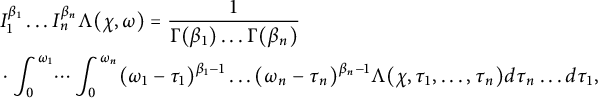 $$ \begin{align*} & I_1^{\beta_1} \dots I_n^{\beta_n} \Lambda(\chi, \omega) = \frac{1}{\Gamma(\beta_1)\dots \Gamma(\beta_n)} \\ & \cdot \int_0^{\omega_1} \dots \int_0^{\omega_n} (\omega_1- \tau_1)^{\beta_1 - 1}\dots (\omega_n- \tau_n)^{\beta_n - 1} \Lambda(\chi, \tau_1, \dots, \tau_n) d \tau_n \dots d \tau_1, \end{align*} $$
where $\Lambda $
is a continuous mapping from
$\Lambda $
is a continuous mapping from $[0, 1] \times [0, 1]^n$
to
$[0, 1] \times [0, 1]^n$
to $\mathbb R$
.
$\mathbb R$
.
In particular, we have
 $$\begin{align*}I_1^0 \dots I_n^0 \Lambda(\chi, \omega) = \Lambda(\chi, \omega) \end{align*}$$
from [Reference Li5].
The partial Liouville–Caputo fractional derivative $_c \partial ^{\alpha }/\partial \chi ^{\alpha }$
of order
$_c \partial ^{\alpha }/\partial \chi ^{\alpha }$
of order $2 < \alpha \leq 3$
with respect to
$2 < \alpha \leq 3$
with respect to $\chi $
is defined in [Reference Kilbas, Srivastava and Trujillo4] as
$\chi $
is defined in [Reference Kilbas, Srivastava and Trujillo4] as
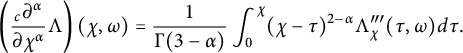 $$\begin{align*}\left(\frac{_c \partial^{\alpha}}{\partial \chi^{\alpha}} \Lambda\right)(\chi, \omega) = \frac{1}{\Gamma(3 - \alpha)} \int_0^\chi (\chi - \tau)^{2 - \alpha} \Lambda_\chi^{\prime\prime\prime}(\tau, \omega) d \tau. \end{align*}$$
One of the most essential subjects of differential equations is the stability theory of Hyers–Ulam [Reference Mohanapriya, Park, Ganesh and Govindan9]. The idea of such stability for differential equations is the substitution of the equation with a given inequality that acts as a perturbation of the equation.
In this paper, we study the uniqueness and Hyers–Ulam stability for the following new fractional nonlinear partial integro-differential equation (FNPIDE) for ${\alpha _{i j} \geq 0\; (i = 1, 2, \dots , n, j = 1, 2, \dots , l \in \mathbb N)}$
:
${\alpha _{i j} \geq 0\; (i = 1, 2, \dots , n, j = 1, 2, \dots , l \in \mathbb N)}$
:
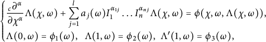 $$ \begin{align} \begin{cases} \displaystyle \frac{ _c \partial^{\alpha}}{\partial \chi^{\alpha}} \Lambda(\chi, \omega) + \sum_{j = 1}^l a_j(\omega) I_1^{\alpha_{1 j}}\dots I_n^{\alpha_{n j}} \Lambda(\chi, \omega) = \phi(\chi, \omega, \Lambda(\chi, \omega)), \\ \Lambda(0, \omega) = \phi_1(\omega), \;\; \Lambda(1, \omega) = \phi_2(\omega), \,\, \Lambda'(1, \omega) = \phi_3(\omega), \end{cases} \end{align} $$
where $(\chi , \omega ) \in [0, 1] \times [0, 1]^n$
,
$(\chi , \omega ) \in [0, 1] \times [0, 1]^n$
, $a_j, \phi _k \in C([0, 1]^n)$
for
$a_j, \phi _k \in C([0, 1]^n)$
for $k = 1, 2, 3$
, and
$k = 1, 2, 3$
, and $\phi : [0, 1] \times [0, 1]^n \times \mathbb R \rightarrow \mathbb R$
satisfies certain conditions to be given later.
$\phi : [0, 1] \times [0, 1]^n \times \mathbb R \rightarrow \mathbb R$
satisfies certain conditions to be given later.
In addition, the operator $I_\chi ^{\alpha }$
is the partial Riemann–Liouville fractional integral of order
$I_\chi ^{\alpha }$
is the partial Riemann–Liouville fractional integral of order $\alpha $
with respect to
$\alpha $
with respect to $\chi $
, given by
$\chi $
, given by
 $$\begin{align*}(I_\chi^{\alpha} \Lambda) (\chi, \omega) = \frac{1}{\Gamma(\alpha)} \int_0^\chi (\chi - \tau)^{\alpha - 1} \Lambda(\tau, \omega) d \tau, \;\; \chi \in [0, 1]. \end{align*}$$
Our main techniques are to derive an equivalent integral equation of equation (1.1) by Babenko’s approach and then to obtain the uniqueness and Hyers–Ulam stability using Banach’s contractive principle and newly established pair-parameter Mittag–Leffler functions below.
Assume $\alpha _{ij} \geq 0, \alpha _i> 0$
for all
$\alpha _{ij} \geq 0, \alpha _i> 0$
for all $i = 1, \dots , n, \, j = 1, \dots , l$
, and there is
$i = 1, \dots , n, \, j = 1, \dots , l$
, and there is $1 \leq i_0 \leq n$
such that
$1 \leq i_0 \leq n$
such that $\alpha _{i_0 j}> 0$
for all
$\alpha _{i_0 j}> 0$
for all $j = 1, \dots , l$
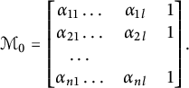
. We define
$j = 1, \dots , l$
. We define
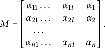 $$ \begin{align} M = \begin{bmatrix} \alpha_{11} \dots & \alpha_{1l} & \alpha_1 \\ \alpha_{21} \dots & \alpha_{2l} & \alpha_2 \\ \dots & & \\ \alpha_{n1} \dots & \alpha_{n l} & \alpha_n \\ \end{bmatrix}. \end{align} $$
Definition 1.1 Let $\beta \geq 0, \; \gamma> 0$
. A pair-parameter
$\beta \geq 0, \; \gamma> 0$
. A pair-parameter $(\beta , \gamma )$
matrix Mittag–Leffler function is defined by
$(\beta , \gamma )$
matrix Mittag–Leffler function is defined by
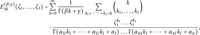 $$ \begin{align*} E_M^{(\beta, \gamma)}(\zeta_1, \dots, \zeta_l) = & \sum_{\mathit{k} = 0}^\infty \frac{1}{\Gamma(\beta k + \gamma)}\sum_{\mathit{k}_1 + \cdots + \mathit{k}_l = \mathit{k} } \binom{\mathit{k}}{\mathit{k}_1, \dots, \mathit{k}_l} \\ & \cdot \frac{\zeta_1^{\mathit{k}_1} \dots \zeta_l^{\mathit{k}_l} }{\Gamma(\alpha_{11} \mathit{k}_1 + \cdots + \alpha_{1 l} \mathit{k}_{l} + \alpha_1) \dots \Gamma(\alpha_{n1} \mathit{k}_1 + \cdots + \alpha_{n l} \mathit{k}_{l} + \alpha_n)}, \end{align*} $$
where $ \zeta _i \in \mathbb {C} $
for
$ \zeta _i \in \mathbb {C} $
for $i = 1, 2, \dots , l$
, and
$i = 1, 2, \dots , l$
, and
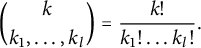 $$\begin{align*}\binom{\mathit{k}}{\mathit{k}_1, \dots, \mathit{k}_l} = \frac{\mathit{k}!}{\mathit{k}_1 ! \dots \mathit{k}_l !}. \end{align*}$$
It follows that
 $$\begin{align*}E_M^{(0, 1)}(\zeta_1, \dots, \zeta_l) = E_M^{(0, 2)}(\zeta_1, \dots, \zeta_l) = E_M(\zeta_1, \dots, \zeta_l), \end{align*}$$
where $E_M$
is a matrix Mittag–Leffler function given in [Reference Li, Beaudin, Rahmoune and Remili6].
$E_M$
is a matrix Mittag–Leffler function given in [Reference Li, Beaudin, Rahmoune and Remili6].
Since there exists a positive constant $\theta $
such that
$\theta $
such that
 $$ \begin{align*} & \Gamma(\beta k + \gamma) \geq \theta, \\ & \Gamma(\alpha_{11} \mathit{k}_1 + \cdots + \alpha_{1 l} \mathit{k}_{l} + \alpha_1) \geq \theta, \\ & \dots, \\ & \Gamma(\alpha_{n1} \mathit{k}_1 + \cdots + \alpha_{n l} \mathit{k}_{l} + \alpha_n) \geq \theta, \end{align*} $$
we claim
 $$ \begin{align*} & \left|E_M^{(\beta, \gamma)}(\zeta_1, \dots, \zeta_l) \right| \\& \quad \leq \frac{1}{\theta^n} \sum_{\mathit{k} = 0}^\infty \sum_{\mathit{k}_1 + \cdots + \mathit{k}_l = \mathit{k} } \binom{\mathit{k}}{\mathit{k}_1, \dots, \mathit{k}_l} \frac{|\zeta_1|^{\mathit{k}_1} \dots |\zeta_l|^{\mathit{k}_l}}{\Gamma(\alpha_{i_0 1} k_1 + \cdots + \alpha_{i_0 l} k_l + \alpha_{i_0})} \\& \quad = \frac{1}{\theta^n} E_{ (\alpha_{i_0 1}, \dots, \alpha_{i_0 l}), \alpha_{i_0}}( |\zeta_l|, \dots, |\zeta_l|) < + \infty, \end{align*} $$
which implies that $E_M^{(\beta , \gamma )}(\zeta _1, \dots , \zeta _l) $
is well defined as the multivariate Mittag–Leffler function
$E_M^{(\beta , \gamma )}(\zeta _1, \dots , \zeta _l) $
is well defined as the multivariate Mittag–Leffler function $E_{ (\alpha _{i_0 1}, \dots , \alpha _{i_0 l}), \alpha _{i_0}}( |\zeta _l|, \dots , |\zeta _l|)$
converges [Reference Hadid and Luchko3]. Obviously,
$E_{ (\alpha _{i_0 1}, \dots , \alpha _{i_0 l}), \alpha _{i_0}}( |\zeta _l|, \dots , |\zeta _l|)$
converges [Reference Hadid and Luchko3]. Obviously,
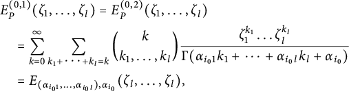 $$ \begin{align*} & E_P^{(0, 1)}(\zeta_1, \dots, \zeta_l) = E_P^{(0, 2)}(\zeta_1, \dots, \zeta_l) \\& \quad = \sum_{\mathit{k} = 0}^\infty \sum_{\mathit{k}_1 + \cdots + \mathit{k}_l = \mathit{k} } \binom{\mathit{k}}{\mathit{k}_1, \dots, \mathit{k}_l} \frac{\zeta_1^{\mathit{k}_1} \dots \zeta_l^{\mathit{k}_l}}{\Gamma(\alpha_{i_0 1} k_1 + \cdots + \alpha_{i_0 l} k_l + \alpha_{i_0})} \\& \quad = E_{ (\alpha_{i_0 1}, \dots, \alpha_{i_0 l}), \alpha_{i_0}}( \zeta_l, \dots, \zeta_l), \end{align*} $$
where
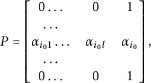 $$\begin{align*}P = \begin{bmatrix} 0 \dots & 0 & 1 \\ \dots & & \\ \alpha_{i_0 1} \dots & \alpha_{i_0 l} & \alpha_{i_0} \\ \dots & & \\ 0 \dots & 0 & 1 \\ \end{bmatrix}, \end{align*}$$
and
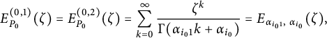 $$\begin{align*}E_{P_0}^{(0, 1)} (\zeta) = E_{P_0}^{(0, 2)} (\zeta) = \sum_{k = 0}^\infty \frac{\zeta^k}{\Gamma(\alpha_{i_0 1} k + \alpha_{i_0})} = E_{\alpha_{i_0 1}, \; \alpha_{i_0} } (\zeta), \end{align*}$$
which is the well-known two-parameter Mittag–Leffler function, and
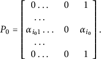 $$\begin{align*}P_0 = \begin{bmatrix} 0 \dots & 0 & 1 \\ \dots & & \\ \alpha_{i_0 1} \dots & 0 & \alpha_{i_0} \\ \dots & & \\ 0 \dots & 0 & 1 \\ \end{bmatrix}. \end{align*}$$
Babenko’s approach (BA) [Reference Babenko1] is a useful tool for dealing with various integral or differential equations (including PDEs) with initial or boundary problems. Let f be a continuous function on $[0, 1] \times \mathbb R$
with
$[0, 1] \times \mathbb R$
with
 $$\begin{align*}{\left\lVert{f}\right\rVert} = \sup_{(x, y) \in [0, 1] \times \mathbb R} |f(x, y)| < + \infty. \end{align*}$$
To demonstrate this method in detail, we convert the following fractional differential equation with a nonlocal initial condition into an equivalent implicit integral equation:
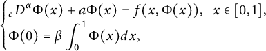 $$ \begin{align} \begin{cases} \displaystyle _c D^{\alpha} \Phi (x) + a \Phi(x) = f(x, \Phi(x)), \;\; x \in [0, 1], \\\Phi(0) = \displaystyle \beta \int_0^1 \Phi(x) d x, \end{cases} \end{align} $$
where $ 0 < \alpha \leq 1$
, a and
$ 0 < \alpha \leq 1$
, a and $ \beta $
are constants.
$ \beta $
are constants.
Evidently, we get by applying the operator $I^{\alpha }$
to equation (1.3)
$I^{\alpha }$
to equation (1.3)
 $$\begin{align*}I^{\alpha} ( _c D^{\alpha} \Phi (x) ) + a I^{\alpha} \Phi(x) = I^{\alpha} f(x, \Phi(x)), \end{align*}$$
which infers that
 $$\begin{align*}\Phi(x) - \Phi(0) + a I^{\alpha} \Phi(x) = I^{\alpha} f(x, \Phi(x)), \end{align*}$$
and
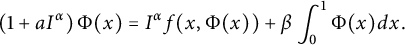 $$ \begin{align*} & \left(1 + a I^{\alpha}\right) \Phi(x) = I^{\alpha} f(x, \Phi(x)) + \beta \int_0^1 \Phi(x) d x. \end{align*} $$
Treating the factor $\left (1 + a I^{\alpha }\right )$
as a variable and using BA, we come to
$\left (1 + a I^{\alpha }\right )$
as a variable and using BA, we come to
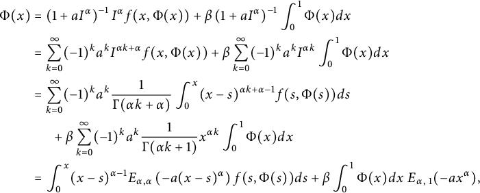 $$ \begin{align*} \Phi(x) & = \left(1 + a I^{\alpha}\right)^{-1} I^{\alpha} f(x, \Phi(x)) + \beta \left(1 + a I^{\alpha}\right)^{-1} \int_0^1 \Phi(x) d x \\ & = \sum_{k = 0}^\infty (-1)^k a^k I^{\alpha k + \alpha} f(x, \Phi(x)) + \beta \sum_{k = 0}^\infty (-1)^k a^k I^{\alpha k } \int_0^1 \Phi(x) d x \\ & = \sum_{k = 0}^\infty (-1)^k a^k \frac{1}{\Gamma(\alpha k + \alpha)} \int_0^x (x - s)^{\alpha k + \alpha - 1} f(s, \Phi(s)) ds \\ & \hspace{0.5cm} + \beta \sum_{k = 0}^\infty (-1)^k a^k \frac{1}{\Gamma(\alpha k + 1)} x^{\alpha k} \int_0^1 \Phi(x) d x \\ & = \int_0^x (x - s)^{\alpha - 1} E_{\alpha, \alpha} \left(- a (x - s)^{\alpha}\right) f(s, \Phi(s)) ds + \beta \int_0^1 \Phi(x) d x \; E_{\alpha, \; 1} ( - a x^{\alpha}), \end{align*} $$
by noting that
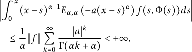 $$ \begin{align*} & \left| \int_0^x (x - s)^{\alpha - 1} E_{\alpha, \alpha} \left(- a (x - s)^{\alpha}\right) f(s, \Phi(s)) ds \right| \\ & \quad \leq \frac{1}{\alpha} {\left\lVert{f}\right\rVert} \sum_{k = 0}^\infty \frac{|a|^k}{\Gamma(\alpha k + \alpha)} < + \infty, \end{align*} $$
and
 $$\begin{align*}\Phi(0) = \beta \int_0^1 \Phi(x) d x. \end{align*}$$
In summary, equation (1.3) is equivalent to the following integral equation:
 $$ \begin{align} \Phi(x) = \int_0^x (x - s)^{\alpha - 1} E_{\alpha, \alpha} \left(- a (x - s)^{\alpha}\right) f(s, \Phi(s)) ds + \beta \int_0^1 \Phi(x) d x \; E_{\alpha, \; 1} ( - a x^{\alpha}). \end{align} $$
The above integral equation, in fact, plays an important role in studying the uniqueness of equation (1.3) in the Banach space $C[0, 1]$
with the norm
$C[0, 1]$
with the norm
 $$\begin{align*}{\left\lVert{\Phi}\right\rVert} = \max_{x \in [0, 1]}|\Phi(x) | < + \infty. \end{align*}$$
We further assume there is a constant $\mathcal L> 0$
such that f satisfies the following Lipschitz condition:
$\mathcal L> 0$
such that f satisfies the following Lipschitz condition:
 $$\begin{align*}| f(x, y_1) - f(x, y_2) | \leq \mathcal L |y_1 - y_2|, \end{align*}$$
and
 $$\begin{align*}\mathcal B = \frac{\mathcal L}{\alpha } E_{\alpha, \alpha }(|a|) + |\beta| E_{\alpha, 1}(|a|) < 1. \end{align*}$$
Then equation (1.3) has a unique solution in $C[0, 1]$
.
$C[0, 1]$
.
To prove this, we define a nonlinear mapping M over $C[0, 1]$
as
$C[0, 1]$
as
 $$ \begin{align*} & (M \Phi) (x) \\ & \quad = \int_0^x (x - s)^{\alpha - 1} E_{\alpha, \alpha} \left(- a (x - s)^{\alpha}\right) f(s, \Phi(s)) ds + \beta \int_0^1 \Phi(x) d x \; E_{\alpha, \; 1} ( - a x^{\alpha}). \end{align*} $$
It follows from the above that $ (M \Phi ) (x) \in C[0, 1]$
. We are going to show that M is contractive. For
$ (M \Phi ) (x) \in C[0, 1]$
. We are going to show that M is contractive. For $\Phi _1, \Phi _2 \in C[0, 1]$
, we have
$\Phi _1, \Phi _2 \in C[0, 1]$
, we have
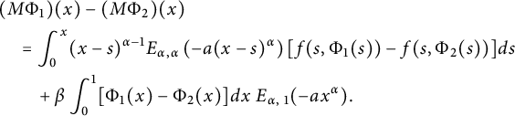 $$ \begin{align*} & (M \Phi_1) (x) - (M \Phi_2) (x) \\ & \quad = \int_0^x (x - s)^{\alpha - 1} E_{\alpha, \alpha} \left(- a (x - s)^{\alpha}\right) [ f(s, \Phi_1(s)) - f(s, \Phi_2(s))] ds \\ & \qquad + \beta \int_0^1 [\Phi_1(x) - \Phi_2(x)] d x \; E_{\alpha, \; 1} ( - a x^{\alpha}). \end{align*} $$
Hence,
 $$\begin{align*}{\left\lVert{M\Phi_1 - M \Phi_2}\right\rVert} \leq \left(\frac{\mathcal L}{\alpha } E_{\alpha, \alpha }(|a|) + |\beta| E_{\alpha, 1}(|a|)\right) {\left\lVert{\Phi_1 - \Phi_2}\right\rVert} = \mathcal B {\left\lVert{\Phi_1 - \Phi_2}\right\rVert}. \end{align*}$$
Since $\mathcal B < 1$
, we claim that equation (1.3) has a unique solution in
$\mathcal B < 1$
, we claim that equation (1.3) has a unique solution in $C[0, 1]$
by Banach’s contractive principle (BCP).
$C[0, 1]$
by Banach’s contractive principle (BCP).
We define $S([0, 1] \times [0, 1]^n)$
as the Banach space of all continuous mappings from
$S([0, 1] \times [0, 1]^n)$
as the Banach space of all continuous mappings from $[0, 1] \times [0, 1]^n$
to
$[0, 1] \times [0, 1]^n$
to $\mathbb R$
with the norm
$\mathbb R$
with the norm
 $$\begin{align*}{\left\lVert{\Lambda}\right\rVert} = \sup_{(\chi, \, \omega) \in [0, 1] \times [0, 1]^n} |\Lambda(\chi, \omega)|, \, \quad \mbox{for}\;\; \Lambda \in S([0, 1] \times [0, 1]^n). \end{align*}$$
Fractional partial differential equations (a generalization of classical PDEs of integer order) are used to model various phenomena in physics, engineering, and other fields. There are intensive studies on fractional PDEs using various approaches, such as integral transforms [Reference Mahor, Mishra and Jain8], analytical and numerical solutions [Reference Momani and Odibat10], homotopy analysis technique [Reference Dehghan and Shakeri2, Reference Singh, Kumar and Swroop11], variational iteration method [Reference Xu, Ling, Zhao and Jassim12] and so on. Very recently, Li et al. [Reference Li, Saadati, O’Regan, Mesiar and Hrytsenko7] investigated the uniqueness of solutions for the following fractional PDE with nonlocal initial value conditions for $2 < \alpha \leq 3$
,
$2 < \alpha \leq 3$
, $0 < \alpha _1 \leq 1$
and
$0 < \alpha _1 \leq 1$
and $ \alpha _2> 0$
based on BCP, BA and the multivariate Mittag–Leffler function for a constant
$ \alpha _2> 0$
based on BCP, BA and the multivariate Mittag–Leffler function for a constant $\eta $
:
$\eta $
:
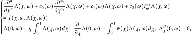 $$ \begin{align*} \begin{cases} \displaystyle \frac{ _c \partial^{\alpha}}{\partial \chi^{\alpha}} \Lambda(\chi, \omega) + c_0(\omega) \frac{ _c \partial^{\alpha_1}}{\partial \chi^{\alpha_1}} \Lambda(\chi, \omega) + c_1 (\omega) \Lambda(\chi, \omega) + c_2(\omega) I_\omega^{\alpha_2} \Lambda(\chi, \omega) \\= f(\chi, \omega, \Lambda(\chi, \omega)), \\ \Lambda(0, \omega) = \displaystyle \eta \int_0^1 \Lambda(\chi, \omega) d \chi, \;\; \displaystyle \frac{ \partial}{\partial \chi} \Lambda(0, \omega) = \int_0^1 \psi(\chi) \Lambda(\chi, \omega) d\chi, \,\, \Lambda^{\prime\prime}_\chi(0, \omega ) = 0, \end{cases} \end{align*} $$
where $(\chi , \omega ) \in [0, 1] \times [0, b]$
,
$(\chi , \omega ) \in [0, 1] \times [0, b]$
, $\psi \in C[0, 1]$
and
$\psi \in C[0, 1]$
and $f: [0, 1] \times [0, b] \times \mathbb R \rightarrow \mathbb R$
satisfies certain conditions.
$f: [0, 1] \times [0, b] \times \mathbb R \rightarrow \mathbb R$
satisfies certain conditions.
We will first convert equation (1.1) into an equivalent implicit integral equation in a series by BA in Section 2, and then further study the uniqueness of solutions via BCP in the space $S([0, 1] \times [0, 1]^n)$
. In Section 3, we derive the Hyers–Ulam stability based on the implicit integral equation and present several examples demonstrating applications of the key results obtained in Section 4. Finally, we summarize the entire work in Section 5.
$S([0, 1] \times [0, 1]^n)$
. In Section 3, we derive the Hyers–Ulam stability based on the implicit integral equation and present several examples demonstrating applications of the key results obtained in Section 4. Finally, we summarize the entire work in Section 5.
2 Uniqueness
We begin converting equation (1.1) to an implicit integral equation then derive sufficient conditions for the uniqueness based on Banach’s contractive principle.
Theorem 2.1 Suppose $a_j, \phi _1, \phi _2, \phi _3 \in C([0, 1]^n)$
for
$a_j, \phi _1, \phi _2, \phi _3 \in C([0, 1]^n)$
for $j = 1, 2, \dots , j$
,
$j = 1, 2, \dots , j$
, $\phi $
is a continuous function on
$\phi $
is a continuous function on $[0, 1] \times [0, 1]^n \times \mathbb R$
with
$[0, 1] \times [0, 1]^n \times \mathbb R$
with
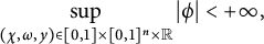 $$\begin{align*}\sup_{(\chi, \omega, y) \in [0, 1] \times [0, 1]^n \times \mathbb R} |\phi| < + \infty, \end{align*}$$ $\alpha _{ij} \geq 0 $
for all
$\alpha _{ij} \geq 0 $
for all $i = 1, \dots , n, \, j = 1, \dots , l$
, and there is
$i = 1, \dots , n, \, j = 1, \dots , l$
, and there is $1 \leq i_0 \leq n$
such that
$1 \leq i_0 \leq n$
such that $\alpha _{i_0 j}> 0$
for all
$\alpha _{i_0 j}> 0$
for all $j = 1, \dots , l$
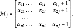
. Furthermore, we assume that
$j = 1, \dots , l$
. Furthermore, we assume that
 $$ \begin{align*} \mathcal M_j = \begin{bmatrix} \alpha_{11} \dots & \alpha_{1l} & \alpha_{1 j}+ 1 \\ \alpha_{21} \dots & \alpha_{2l} & \alpha_{2 j} + 1\\ \dots & & \\ \alpha_{n1} \dots & \alpha_{n l} & \alpha_{n j } + 1 \\ \end{bmatrix}, \end{align*} $$
and
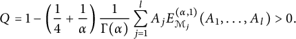 $$\begin{align*}Q = 1 - \left(\frac{1}{4} + \frac{1}{\alpha} \right) \frac{1}{\Gamma(\alpha)}\sum_{j = 1}^l A_j E_{\mathcal M_j}^{(\alpha, 1 )}(A_1, \dots, A_l)> 0. \end{align*}$$
Then equation (1.1) is equivalent to the following implicit integral equation:
 $$ \begin{align} \Lambda & = \sum_{k = 1}^\infty (-1)^k \sum_{k_1 + \cdots + k_l = k} \binom{k}{k_1, \dots, k_l}\left(a_1 (\omega) I_\chi^{\alpha} I_1^{\alpha_{1 1}}\dots I_n^{\alpha_{n 1}}\right)^{k_1}\cdots \left( a_l (\omega) I_\chi^{\alpha} I_1^{\alpha_{1 l}}\dots I_n^{\alpha_{n l}}\right)^{k_l} \nonumber \\& \quad \cdot ( \phi_1 (\omega) (1- 2 \chi + \chi^2) + \phi_2 (\omega) (2 \chi - \chi^2 ) + \phi_3 (\omega) (\chi^2 - \chi) + I_{\chi = 1}^{\alpha - 1} (\chi \phi - \chi^2 \phi) \nonumber \\& \quad + I_{\chi = 1}^{\alpha} (\chi^2 \phi - 2 \chi \phi) + I_\chi^{\alpha} \phi + \sum_{j = 1}^l a_j(\omega) I_1^{\alpha_{1 j}}\dots I_n^{\alpha_{n j}} I_{\chi = 1}^{\alpha - 1} (\chi \Lambda - \chi^2 \Lambda) \nonumber \\& \quad + \sum_{j = 1}^l a_j(\omega) I_1^{\alpha_{1 j}}\dots I_n^{\alpha_{n j}} I_{\chi = 1}^{\alpha } (\chi^2 \Lambda - 2 \chi \Lambda) ).\nonumber \\ \end{align} $$
In addition, $\Lambda $
is a uniformly bounded function satisfying
$\Lambda $
is a uniformly bounded function satisfying
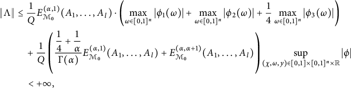
 $$ \begin{align*} {\left\lVert{\Lambda}\right\rVert} &\leq \frac{1}{Q} E_{\mathcal M_0}^{(\alpha, 1 )}(A_1, \dots, A_l) \cdot \left (\max_{\omega \in [0, 1]^n} |\phi_1 (\omega)| + \max_{\omega \in [0, 1]^n} |\phi_2 (\omega)| + \frac{1}{4} \max_{\omega \in [0, 1]^n} |\phi_3 (\omega)|\right) \\& \quad + \frac{1}{Q} \left(\frac{\displaystyle \frac{1}{4} + \frac{1}{\alpha}}{\Gamma(\alpha)} E_{\mathcal M_0}^{(\alpha, 1 )}(A_1, \dots, A_l) + E_{\mathcal M_0}^{(\alpha, \alpha + 1 )}(A_1, \dots, A_l)\right) \sup_{(\chi, \omega, y) \in [0, 1] \times [0, 1]^n \times \mathbb R} |\phi| \\& \quad < + \infty, \end{align*} $$
where
 $$ \begin{align*} \mathcal M_0 = \begin{bmatrix} \alpha_{11} \dots & \alpha_{1l} & 1 \\ \alpha_{21} \dots & \alpha_{2l} & 1\\ \dots & & \\ \alpha_{n1} \dots & \alpha_{n l} & 1 \\ \end{bmatrix}. \end{align*} $$
Proof It follows from [Reference Li, Saadati, O’Regan, Mesiar and Hrytsenko7] that
 $$ \begin{align*} I_\chi^{\alpha} \left(\displaystyle \frac{ _c \partial^{\alpha}}{\partial \chi^{\alpha}} \Lambda \right) (\chi, \omega) = \Lambda(\chi, \omega) - \Lambda(0, \omega) -\Lambda^{\prime}_\chi(0, \omega) \chi - \Lambda_\chi^{"}(0, \omega) \frac{\chi^2}{2}, \end{align*} $$
where $0 < \alpha \leq 3$
.
$0 < \alpha \leq 3$
.
Applying the integral operator $ I_\chi ^{\alpha } $
to equation (1.1) and using the condition
$ I_\chi ^{\alpha } $
to equation (1.1) and using the condition $\Lambda (0, \omega ) = \phi _1(\omega )$
, we get
$\Lambda (0, \omega ) = \phi _1(\omega )$
, we get
 $$ \begin{align} & \Lambda(\chi, \omega) - \phi_1(\omega) -\Lambda^{\prime}_\chi(0, \omega) \chi - \Lambda_\chi^{"}(0, \omega) \frac{\chi^2}{2} \nonumber \\ & \quad + \sum_{j = 1}^l a_j(\omega) I_\chi^{\alpha} I_1^{\alpha_{1 j}}\dots I_n^{\alpha_{n j}} \Lambda(\chi, \omega) = I_\chi^{\alpha} \phi(\chi, \omega, \Lambda(\chi, \omega)). \end{align} $$
Setting $\chi = 1$
, we come to
$\chi = 1$
, we come to
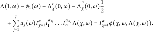 $$ \begin{align} & \Lambda(1, \omega) - \phi_1(\omega) -\Lambda^{\prime}_\chi(0, \omega) - \Lambda_\chi^{"}(0, \omega) \frac{1}{2} \nonumber \\ & \quad + \sum_{j = 1}^l a_j(\omega) I_{\chi = 1}^{\alpha} I_1^{\alpha_{1 j}}\dots I_n^{\alpha_{n j}} \Lambda(\chi, \omega) = I_{\chi = 1}^{\alpha} \phi(\chi, \omega, \Lambda(\chi, \omega)). \end{align} $$
Differentiating equation (2.2) with respect to $\chi $
, we deduce that for
$\chi $
, we deduce that for $\chi = 1$
,
$\chi = 1$
,
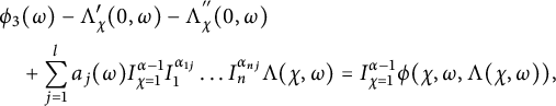 $$ \begin{align} & \phi_3(\omega) -\Lambda^{\prime}_\chi(0, \omega) - \Lambda_\chi^{"}(0, \omega) \nonumber \\ & \quad + \sum_{j = 1}^l a_j(\omega) I_{\chi = 1}^{\alpha -1} I_1^{\alpha_{1 j}}\dots I_n^{\alpha_{n j}} \Lambda(\chi, \omega) = I_{\chi = 1}^{\alpha -1} \phi(\chi, \omega, \Lambda(\chi, \omega)), \end{align} $$
by the given initial condition.
From equations (2.3) and (2.4), we derive that
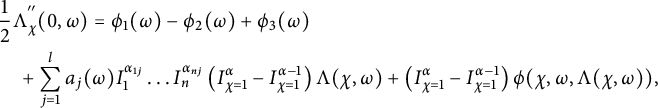 $$ \begin{align*} & \frac{1}{2} \Lambda_\chi^{"}(0, \omega) = \phi_1(\omega) - \phi_2(\omega) + \phi_3(\omega) \\ & \quad + \sum_{j = 1}^l a_j(\omega) I_1^{\alpha_{1 j}}\dots I_n^{\alpha_{n j}} \left(I_{\chi = 1}^{\alpha} - I_{\chi = 1}^{\alpha - 1} \right)\Lambda(\chi, \omega) + \left(I_{\chi = 1}^{\alpha} - I_{\chi = 1}^{\alpha - 1} \right)\phi(\chi, \omega, \Lambda(\chi, \omega)), \end{align*} $$
and
 $$ \begin{align*} & \Lambda^{\prime}_\chi (0, \omega) = 2 \phi_2(\omega) - 2 \phi_1(\omega) - \phi_3(\omega) \\ & \quad + \sum_{j = 1}^l a_j(\omega) I_1^{\alpha_{1 j}}\dots I_n^{\alpha_{n j}} \left(I_{\chi = 1}^{\alpha - 1} - 2 I_{\chi = 1}^{\alpha } \right)\Lambda(\chi, \omega) + \left(I_{\chi = 1}^{\alpha - 1} - 2 I_{\chi = 1}^{\alpha } \right)\phi(\chi, \omega, \Lambda(\chi, \omega)). \end{align*} $$
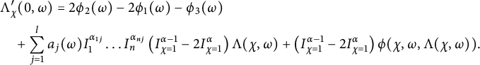
Hence,
 $$ \begin{align*} & \left(1 + \sum_{j = 1}^l a_j(\omega) I_\chi^{\alpha} I_1^{\alpha_{1 j}}\dots I_n^{\alpha_{n j}} \right)\Lambda(\chi, \omega) \\ & \quad = \phi_1 (\omega) (1- 2 \chi + \chi^2) + \phi_2 (\omega) (2 \chi - \chi^2 ) + \phi_3 (\omega) (\chi^2 - \chi) + I_{\chi = 1}^{\alpha - 1} (\chi \phi - \chi^2 \phi) \\ & \qquad + I_{\chi = 1}^{\alpha} (\chi^2 \phi - 2 \chi \phi) + I_\chi^{\alpha} \phi + \sum_{j = 1}^l a_j(\omega) I_1^{\alpha_{1 j}}\dots I_n^{\alpha_{n j}} I_{\chi = 1}^{\alpha - 1} (\chi \Lambda - \chi^2 \Lambda) \\ & \qquad + \sum_{j = 1}^l a_j(\omega) I_1^{\alpha_{1 j}}\dots I_n^{\alpha_{n j}} I_{\chi = 1}^{\alpha } (\chi^2 \Lambda - 2 \chi \Lambda). \end{align*} $$
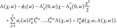
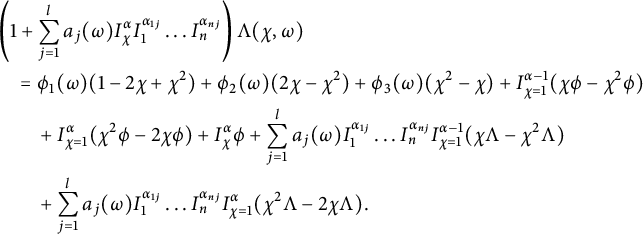
Using BA, we deduce that
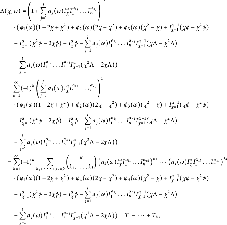 $$ \begin{align*} & \Lambda(\chi, \omega) = \left(1 + \sum_{j = 1}^l a_j(\omega) I_\chi^{\alpha} I_1^{\alpha_{1 j}}\dots I_n^{\alpha_{n j}} \right)^{-1} \\& \qquad \cdot ( \phi_1 (\omega) (1- 2 \chi + \chi^2) + \phi_2 (\omega) (2 \chi - \chi^2 ) + \phi_3 (\omega) (\chi^2 - \chi) + I_{\chi = 1}^{\alpha - 1} (\chi \phi - \chi^2 \phi) \\& \qquad + I_{\chi = 1}^{\alpha} (\chi^2 \phi - 2 \chi \phi) + I_\chi^{\alpha} \phi + \sum_{j = 1}^l a_j(\omega) I_1^{\alpha_{1 j}}\dots I_n^{\alpha_{n j}} I_{\chi = 1}^{\alpha - 1} (\chi \Lambda - \chi^2 \Lambda) \\& \qquad + \sum_{j = 1}^l a_j(\omega) I_1^{\alpha_{1 j}}\dots I_n^{\alpha_{n j}} I_{\chi = 1}^{\alpha } (\chi^2 \Lambda - 2 \chi \Lambda) ) \\& \quad = \sum_{k = 1}^\infty (-1)^k \left(\sum_{j = 1}^l a_j(\omega) I_\chi^{\alpha} I_1^{\alpha_{1 j}}\dots I_n^{\alpha_{n j}} \right)^k \\& \qquad \cdot ( \phi_1 (\omega) (1- 2 \chi + \chi^2) + \phi_2 (\omega) (2 \chi - \chi^2 ) + \phi_3 (\omega) (\chi^2 - \chi) + I_{\chi = 1}^{\alpha - 1} (\chi \phi - \chi^2 \phi) \\& \qquad + I_{\chi = 1}^{\alpha} (\chi^2 \phi - 2 \chi \phi) + I_\chi^{\alpha} \phi + \sum_{j = 1}^l a_j(\omega) I_1^{\alpha_{1 j}}\dots I_n^{\alpha_{n j}} I_{\chi = 1}^{\alpha - 1} (\chi \Lambda - \chi^2 \Lambda) \\& \qquad + \sum_{j = 1}^l a_j(\omega) I_1^{\alpha_{1 j}}\dots I_n^{\alpha_{n j}} I_{\chi = 1}^{\alpha } (\chi^2 \Lambda - 2 \chi \Lambda) ) \\& \quad = \sum_{k = 1}^\infty (-1)^k \sum_{k_1 + \cdots + k_l = k} \binom{k}{k_1, \dots, k_l}\left(a_1 (\omega) I_\chi^{\alpha} I_1^{\alpha_{1 1}}\dots I_n^{\alpha_{n 1}}\right)^{k_1}\cdots \left( a_l (\omega) I_\chi^{\alpha} I_1^{\alpha_{1 l}}\dots I_n^{\alpha_{n l}}\right)^{k_l} \\& \qquad \cdot ( \phi_1 (\omega) (1- 2 \chi + \chi^2) + \phi_2 (\omega) (2 \chi - \chi^2 ) + \phi_3 (\omega) (\chi^2 - \chi) + I_{\chi = 1}^{\alpha - 1} (\chi \phi - \chi^2 \phi) \\& \qquad + I_{\chi = 1}^{\alpha} (\chi^2 \phi - 2 \chi \phi) + I_\chi^{\alpha} \phi + \sum_{j = 1}^l a_j(\omega) I_1^{\alpha_{1 j}}\dots I_n^{\alpha_{n j}} I_{\chi = 1}^{\alpha - 1} (\chi \Lambda - \chi^2 \Lambda) \\& \qquad + \sum_{j = 1}^l a_j(\omega) I_1^{\alpha_{1 j}}\dots I_n^{\alpha_{n j}} I_{\chi = 1}^{\alpha } (\chi^2 \Lambda - 2 \chi \Lambda) ) = T_1 + \cdots + T_8, \end{align*} $$
where
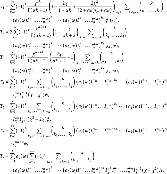 $$ \begin{align*} T_1 &= \sum_{k = 1}^\infty (-1)^k \frac{\chi^{\alpha k}}{\Gamma(\alpha k + 1)} \left(1 - \frac{2 \chi}{1 + \alpha k} + \frac{2 \chi^2}{(2 + \alpha k)(1 + \alpha k)} \right) \sum_{k_1 + \cdots + k_l = k} \binom{k}{k_1, \dots, k_l} \\& \quad \cdot \left(a_1 (\omega) I_1^{\alpha_{1 1}}\dots I_n^{\alpha_{n 1}}\right)^{k_1} \cdots \left(a_l (\omega) I_1^{\alpha_{1 l}}\dots I_n^{\alpha_{n l}}\right)^{k_l} \phi_1 (\omega), \\T_2 &= 2 \sum_{k = 1}^\infty (-1)^k \frac{\chi^{\alpha k + 1}}{\Gamma(\alpha k + 2)} \left(1 - \frac{\chi}{\alpha k + 2} \right) \sum_{k_1 + \cdots + k_l = k} \binom{k}{k_1, \dots, k_l} \\& \quad \cdot \left(a_1 (\omega) I_1^{\alpha_{1 1}}\dots I_n^{\alpha_{n 1}}\right)^{k_1} \cdots \left(a_l (\omega) I_1^{\alpha_{1 l}}\dots I_n^{\alpha_{n l}}\right)^{k_l} \phi_2 (\omega),\\T_3 &= \sum_{k = 1}^\infty (-1)^k \frac{\chi^{\alpha k + 1}}{\Gamma(\alpha k + 2)} \left( \frac{2 \chi}{\alpha k + 2} - 1 \right) \sum_{k_1 + \cdots + k_l = k} \binom{k}{k_1, \dots, k_l} \\& \quad \cdot \left(a_1 (\omega) I_1^{\alpha_{1 1}}\dots I_n^{\alpha_{n 1}}\right)^{k_1} \cdots \left(a_l (\omega) I_1^{\alpha_{1 l}}\dots I_n^{\alpha_{n l}}\right)^{k_l} \phi_3 (\omega),\\T_4 &= \sum_{k = 1}^\infty (-1)^k \sum_{k_1 + \cdots + k_l = k} \binom{k}{k_1, \dots, k_l} \left(a_1 (\omega) I_1^{\alpha_{1 1}}\dots I_n^{\alpha_{n 1}}\right)^{k_1} \cdots \left(a_l (\omega) I_1^{\alpha_{1 l}}\dots I_n^{\alpha_{n l}}\right)^{k_l} \\& \quad \cdot I_\chi^{\alpha k }I_{\chi = 1}^{\alpha -1} (\chi - \chi^2 ) \phi,\\T_5 &= \sum_{k = 1}^\infty (-1)^k \sum_{k_1 + \cdots + k_l = k} \binom{k}{k_1, \dots, k_l} \left(a_1 (\omega) I_1^{\alpha_{1 1}}\dots I_n^{\alpha_{n 1}}\right)^{k_1} \cdots \left(a_l (\omega) I_1^{\alpha_{1 l}}\dots I_n^{\alpha_{n l}}\right)^{k_l} \\& \quad \cdot I_\chi^{\alpha k }I_{\chi = 1}^{\alpha} (\chi^2 - 2 \chi ) \phi,\\T_6 &= \sum_{k = 1}^\infty (-1)^k \sum_{k_1 + \cdots + k_l = k} \binom{k}{k_1, \dots, k_l} \left(a_1 (\omega) I_1^{\alpha_{1 1}}\dots I_n^{\alpha_{n 1}}\right)^{k_1} \cdots \left(a_l (\omega) I_1^{\alpha_{1 l}}\dots I_n^{\alpha_{n l}}\right)^{k_l} \\& \quad \cdot I_\chi^{\alpha k + \alpha} \phi,\\T_7 &= \sum_{j = 1}^l a_j(\omega) \sum_{k = 1}^\infty (-1)^k \sum_{k_1 + \cdots + k_l = k} \binom{k}{k_1, \dots, k_l} \\& \quad \cdot \left(a_1 (\omega) I_1^{\alpha_{1 1}}\dots I_n^{\alpha_{n 1}}\right)^{k_1} \cdots \left(a_l (\omega) I_l^{\alpha_{1 l}}\dots I_n^{\alpha_{n l}}\right)^{k_l} I_\chi^{\alpha k} I_1^{\alpha_{1 j}} \dots I_n^{\alpha_{n j}} I_\chi^{ \alpha - 1} (\chi - \chi^2)\Lambda,\end{align*} $$
and finally,
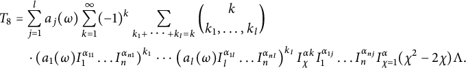 $$ \begin{align*}T_8 &= \sum_{j = 1}^l a_j(\omega) \sum_{k = 1}^\infty (-1)^k \sum_{k_1 + \cdots + k_l = k} \binom{k}{k_1, \dots, k_l} \\& \quad \cdot \left(a_1 (\omega) I_1^{\alpha_{1 1}}\dots I_n^{\alpha_{n 1}}\right)^{k_1} \cdots \left(a_l (\omega) I_l^{\alpha_{1 l}}\dots I_n^{\alpha_{n l}}\right)^{k_l} I_\chi^{\alpha k} I_1^{\alpha_{1 j}} \dots I_n^{\alpha_{n j}} I_{\chi = 1}^{ \alpha } (\chi^2 - 2 \chi)\Lambda.\end{align*} $$
Let
 $$ \begin{align*} & \max_{\omega \in [0, 1]^n} | a_j (\omega)| = A_j, \, \, j = 1, 2, \dots, l, \\ & \max_{\chi \in [0, 1]} | 1 - 2 \chi + \chi^2| = 1, \;\; \max_{\chi \in [0, 1]} | 2 \chi - \chi^2| = 1, \,\, \max_{\chi \in [0, 1]} | \chi^2 - \chi| = \frac{1}{4}. \end{align*} $$
Thus,
 $$ \begin{align*} {\left\lVert{\Lambda}\right\rVert} & \leq \sum_{\mathit{k} = 0}^\infty \frac{1}{\Gamma(\alpha k + 1)}\sum_{\mathit{k}_1 + \cdots + \mathit{k}_l = \mathit{k} } \binom{\mathit{k}}{\mathit{k}_1, \dots, \mathit{k}_l} \\& \quad \cdot \frac{A_1^{\mathit{k}_1} \dots A_l^{\mathit{k}_l} }{\Gamma(\alpha_{11} \mathit{k}_1 + \cdots + \alpha_{1 l} \mathit{k}_{l} + 1) \dots \Gamma(\alpha_{n1} \mathit{k}_1 + \cdots + \alpha_{n l} \mathit{k}_{l} + 1)} \\& \quad \cdot \left (\max_{\omega \in [0, 1]^n} |\phi_1 (\omega)| + \max_{\omega \in [0, 1]^n} |\phi_2 (\omega)| + \frac{1}{4} \max_{\omega \in [0, 1]^n} |\phi_3 (\omega)|\right) + T_{21} + T_{22} + T_{23}, \end{align*} $$
where
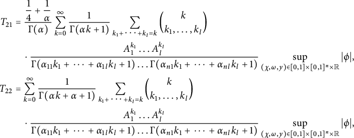 $$ \begin{align*} T_{21} &= \frac{\displaystyle \frac{1}{4} + \frac{1}{\alpha}}{\Gamma(\alpha)} \sum_{\mathit{k} = 0}^\infty \frac{1}{\Gamma(\alpha k + 1)}\sum_{\mathit{k}_1 + \cdots + \mathit{k}_l = \mathit{k} } \binom{\mathit{k}}{\mathit{k}_1, \dots, \mathit{k}_l} \\& \quad \cdot \frac{A_1^{\mathit{k}_1} \dots A_l^{\mathit{k}_l} }{\Gamma(\alpha_{11} \mathit{k}_1 + \cdots + \alpha_{1 l} \mathit{k}_{l} + 1) \dots \Gamma(\alpha_{n1} \mathit{k}_1 + \cdots + \alpha_{n l} \mathit{k}_{l} + 1)} \sup_{(\chi, \omega, y) \in [0, 1] \times [0, 1]^n \times \mathbb R} |\phi|,\\T_{22} &= \sum_{\mathit{k} = 0}^\infty \frac{1}{\Gamma(\alpha k + \alpha + 1)}\sum_{\mathit{k}_1 + \cdots + \mathit{k}_l = \mathit{k} } \binom{\mathit{k}}{\mathit{k}_1, \dots, \mathit{k}_l} \\& \quad \cdot \frac{A_1^{\mathit{k}_1} \dots A_l^{\mathit{k}_l} }{\Gamma(\alpha_{11} \mathit{k}_1 + \cdots + \alpha_{1 l} \mathit{k}_{l} + 1) \dots \Gamma(\alpha_{n1} \mathit{k}_1 + \cdots + \alpha_{n l} \mathit{k}_{l} + 1)} \sup_{(\chi, \omega, y) \in [0, 1] \times [0, 1]^n \times \mathbb R} |\phi|, \end{align*} $$
and
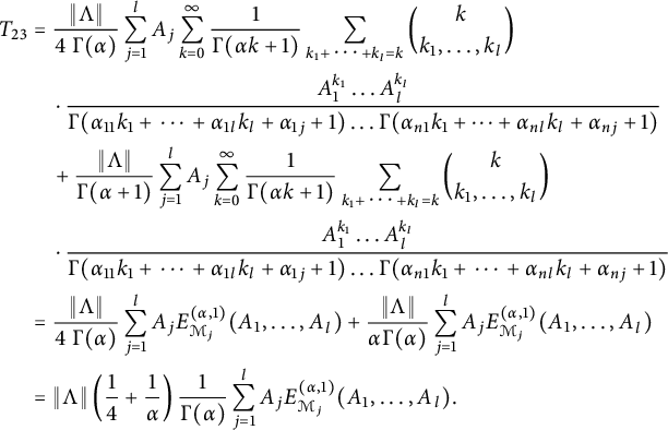 $$ \begin{align*} T_{23} & = \frac{{\left\lVert{\Lambda}\right\rVert}}{4 \; \Gamma(\alpha)} \sum_{j = 1}^l A_j \sum_{\mathit{k} = 0}^\infty \frac{1}{\Gamma(\alpha k + 1)}\sum_{\mathit{k}_1 + \cdots + \mathit{k}_l = \mathit{k} } \binom{\mathit{k}}{\mathit{k}_1, \dots, \mathit{k}_l} \\& \quad \cdot \frac{A_1^{\mathit{k}_1} \dots A_l^{\mathit{k}_l} }{\Gamma(\alpha_{11} \mathit{k}_1 + \cdots + \alpha_{1 l} \mathit{k}_{l} + \alpha_{1 j}+ 1) \dots \Gamma(\alpha_{n1} \mathit{k}_1 + \dots + \alpha_{n l} \mathit{k}_{l} + \alpha_{n j } + 1)} \\& \quad + \frac{{\left\lVert{\Lambda}\right\rVert}}{ \Gamma(\alpha + 1)} \sum_{j = 1}^l A_j \sum_{\mathit{k} = 0}^\infty \frac{1}{\Gamma(\alpha k + 1)}\sum_{\mathit{k}_1 + \cdots + \mathit{k}_l = \mathit{k} } \binom{\mathit{k}}{\mathit{k}_1, \dots, \mathit{k}_l} \\& \quad \cdot \frac{A_1^{\mathit{k}_1} \dots A_l^{\mathit{k}_l} }{\Gamma(\alpha_{11} \mathit{k}_1 + \cdots + \alpha_{1 l} \mathit{k}_{l} + \alpha_{1 j}+ 1) \dots \Gamma(\alpha_{n1} \mathit{k}_1 + \cdots + \alpha_{n l} \mathit{k}_{l} + \alpha_{n j } + 1)} \\& = \frac{{\left\lVert{\Lambda}\right\rVert}}{4 \; \Gamma(\alpha)} \sum_{j = 1}^l A_j E_{\mathcal M_j}^{(\alpha, 1 )}(A_1, \dots, A_l) + \frac{{\left\lVert{\Lambda}\right\rVert}}{\alpha \Gamma(\alpha)} \sum_{j = 1}^l A_j E_{\mathcal M_j}^{(\alpha, 1 )}(A_1, \dots, A_l) \\& = {\left\lVert{\Lambda}\right\rVert} \left(\frac{1}{4} + \frac{1}{\alpha} \right) \frac{1}{\Gamma(\alpha)}\sum_{j = 1}^l A_j E_{\mathcal M_j}^{(\alpha, 1 )}(A_1, \dots, A_l). \end{align*} $$
Using our assumption
 $$\begin{align*}Q = 1 - \left(\frac{1}{4} + \frac{1}{\alpha} \right) \frac{1}{\Gamma(\alpha)}\sum_{j = 1}^l A_j E_{\mathcal M_j}^{(\alpha, 1 )}(A_1, \dots, A_l)> 0, \end{align*}$$
we claim that
 $$ \begin{align*} {\left\lVert{\Lambda}\right\rVert} &\leq \frac{1}{Q} E_{\mathcal M_0}^{(\alpha, 1 )}(A_1, \dots, A_l) \cdot \left (\max_{\omega \in [0, 1]^n} |\phi_1 (\omega)| + \max_{\omega \in [0, 1]^n} |\phi_2 (\omega)| + \frac{1}{4} \max_{\omega \in [0, 1]^n} |\phi_3 (\omega)|\right) \\& \quad + \frac{1}{Q} \left(\frac{\displaystyle \frac{1}{4} + \frac{1}{\alpha}}{\Gamma(\alpha)} E_{\mathcal M_0}^{(\alpha, 1 )}(A_1, \dots, A_l) + E_{\mathcal M_0}^{(\alpha, \alpha + 1 )}(A_1, \dots, A_l)\right) \sup_{(\chi, \omega, y) \in [0, 1] \times [0, 1]^n \times \mathbb R} |\phi| \\& \quad < + \infty, \end{align*} $$
which indicates that $\Lambda $
is a uniformly bounded function. This completes the proof of Theorem 2.1.
$\Lambda $
is a uniformly bounded function. This completes the proof of Theorem 2.1.
Theorem 2.2 Suppose $a_j, \phi _1, \phi _2, \phi _3 \in C([0, 1]^n)$
for
$a_j, \phi _1, \phi _2, \phi _3 \in C([0, 1]^n)$
for $j = 1, 2, \dots , j$
,
$j = 1, 2, \dots , j$
, $\phi $
is a continuous and bounded function on
$\phi $
is a continuous and bounded function on $[0, 1] \times [0, 1]^n \times \mathbb R$
, satisfying the Lipschitz condition for a positive constant
$[0, 1] \times [0, 1]^n \times \mathbb R$
, satisfying the Lipschitz condition for a positive constant $\mathcal C$
 $$\begin{align*}| \phi (\chi, \omega, y_1) - \phi (\chi, \omega, y_2) | \leq \mathcal C |y_1 - y_2|, \;\; y_1, y_2 \in \mathbb R, \end{align*}$$ $\alpha _{ij} \geq 0 $
for all
$\alpha _{ij} \geq 0 $
for all $i = 1, \dots , n, \, j = 1, \dots , l$
, and there is
$i = 1, \dots , n, \, j = 1, \dots , l$
, and there is $1 \leq i_0 \leq n$
such that
$1 \leq i_0 \leq n$
such that $\alpha _{i_0 j}> 0$
for all
$\alpha _{i_0 j}> 0$
for all $j = 1, \dots , l$
. Furthermore, we assume that
$j = 1, \dots , l$
. Furthermore, we assume that
 $$ \begin{align*} \mathcal M_j = \begin{bmatrix} \alpha_{11} \dots & \alpha_{1l} & \alpha_{1 j}+ 1 \\ \alpha_{21} \dots & \alpha_{2l} & \alpha_{2 j} + 1\\ \dots & & \\ \alpha_{n1} \dots & \alpha_{n l} & \alpha_{n j } + 1 \\ \end{bmatrix}, \end{align*} $$
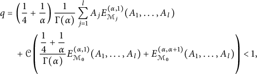
and
 $$ \begin{align*} q &= \left(\frac{1}{4} + \frac{1}{\alpha} \right) \frac{1}{\Gamma(\alpha)}\sum_{j = 1}^l A_j E_{\mathcal M_j}^{(\alpha, 1 )}(A_1, \dots, A_l) \\ & \quad + \mathcal C \left(\frac{\displaystyle \frac{1}{4} + \frac{1}{\alpha}}{\Gamma(\alpha)} E_{\mathcal M_0}^{(\alpha, 1 )}(A_1, \dots, A_l) + E_{\mathcal M_0}^{(\alpha, \alpha + 1 )}(A_1, \dots, A_l)\right) < 1, \end{align*} $$
where
 $$ \begin{align*} \mathcal M_0 = \begin{bmatrix} \alpha_{11} \dots & \alpha_{1l} & 1 \\ \alpha_{21} \dots & \alpha_{2l} & 1\\ \dots & & \\ \alpha_{n1} \dots & \alpha_{n l} & 1 \\ \end{bmatrix}. \end{align*} $$
Then equation (1.1) has a unique uniformly bounded solution in the space $S([0, 1] \times [0, 1]^n).$
Proof We define a nonlinear mapping $\mathcal F$
over
$\mathcal F$
over $S([0, 1] \times [0, 1]^n)$
as
$S([0, 1] \times [0, 1]^n)$
as
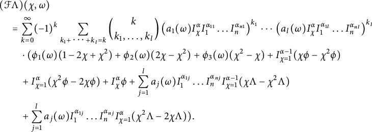 $$ \begin{align*} & (\mathcal F \Lambda)(\chi, \omega) \\& \quad = \sum_{k = 0}^\infty (-1)^k \sum_{k_1 + \cdots + k_l = k} \binom{k}{k_1, \dots, k_l}\left(a_1 (\omega) I_\chi^{\alpha} I_1^{\alpha_{1 1}}\dots I_n^{\alpha_{n 1}}\right)^{k_1}\cdots \left( a_l (\omega) I_\chi^{\alpha} I_1^{\alpha_{1 l}}\dots I_n^{\alpha_{n l}}\right)^{k_l} \nonumber \\& \qquad \cdot ( \phi_1 (\omega) (1- 2 \chi + \chi^2) + \phi_2 (\omega) (2 \chi - \chi^2 ) + \phi_3 (\omega) (\chi^2 - \chi) + I_{\chi = 1}^{\alpha - 1} (\chi \phi - \chi^2 \phi) \nonumber \\& \qquad + I_{\chi = 1}^{\alpha} (\chi^2 \phi - 2 \chi \phi) + I_\chi^{\alpha} \phi + \sum_{j = 1}^l a_j(\omega) I_1^{\alpha_{1 j}}\dots I_n^{\alpha_{n j}} I_{\chi = 1}^{\alpha - 1} (\chi \Lambda - \chi^2 \Lambda) \nonumber \\& \qquad + \sum_{j = 1}^l a_j(\omega) I_1^{\alpha_{1 j}}\dots I_n^{\alpha_{n j}} I_{\chi = 1}^{\alpha } (\chi^2 \Lambda - 2 \chi \Lambda) ). \end{align*} $$
It follows from the proof of Theorem 2.1 that $(\mathcal F \Lambda ) \in S([0, 1] \times [0, 1]^n)$
. We shall show that
$(\mathcal F \Lambda ) \in S([0, 1] \times [0, 1]^n)$
. We shall show that $\mathcal F$
is contractive. Indeed, for
$\mathcal F$
is contractive. Indeed, for $\Lambda _1, \, \Lambda _2 \in S([0, 1] \times [0, 1]^n)$
, we have
$\Lambda _1, \, \Lambda _2 \in S([0, 1] \times [0, 1]^n)$
, we have
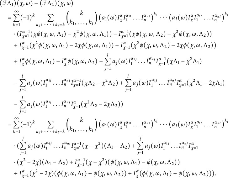 $$ \begin{align*} & (\mathcal F \Lambda_1)(\chi, \omega) - (\mathcal F \Lambda_2)(\chi, \omega) \\& \quad = \sum_{k = 1}^\infty (-1)^k \sum_{k_1 + \cdots + k_l = k} \binom{k}{k_1, \dots, k_l}\left(a_1 (\omega) I_\chi^{\alpha} I_1^{\alpha_{1 1}}\dots I_n^{\alpha_{n 1}}\right)^{k_1}\cdots \left( a_l (\omega) I_\chi^{\alpha} I_1^{\alpha_{1 l}}\dots I_n^{\alpha_{n l}}\right)^{k_l} \nonumber \\& \qquad \cdot ( I_{\chi = 1}^{\alpha - 1} (\chi \phi (\chi, \omega, \Lambda_1) - \chi^2 \phi(\chi, \omega, \Lambda_1 )) - I_{\chi = 1}^{\alpha - 1} (\chi \phi (\chi, \omega, \Lambda_2) - \chi^2 \phi(\chi, \omega, \Lambda_2 )) \\& \qquad + I_{\chi = 1}^{\alpha} (\chi^2 \phi (\chi, \omega, \Lambda_1) - 2 \chi \phi (\chi, \omega, \Lambda_1)) - I_{\chi = 1}^{\alpha} (\chi^2 \phi (\chi, \omega, \Lambda_2) - 2 \chi \phi (\chi, \omega, \Lambda_2)) \\& \qquad + I_\chi^{\alpha} \phi (\chi, \omega, \Lambda_1) - I_\chi^{\alpha} \phi (\chi, \omega, \Lambda_2 ) + \sum_{j = 1}^l a_j(\omega) I_1^{\alpha_{1 j}}\dots I_n^{\alpha_{n j}} I_{\chi = 1}^{\alpha - 1} (\chi \Lambda_1 - \chi^2 \Lambda_1) \\& \qquad - \sum_{j = 1}^l a_j(\omega) I_1^{\alpha_{1 j}}\dots I_n^{\alpha_{n j}} I_{\chi = 1}^{\alpha - 1} (\chi \Lambda_2 - \chi^2 \Lambda_2) + \sum_{j = 1}^l a_j(\omega) I_1^{\alpha_{1 j}}\dots I_n^{\alpha_{n j}} I_{\chi = 1}^{\alpha } (\chi^2 \Lambda_1 - 2 \chi \Lambda_1) \\& \qquad - \sum_{j = 1}^l a_j(\omega) I_1^{\alpha_{1 j}}\dots I_n^{\alpha_{n j}} I_{\chi = 1}^{\alpha } (\chi^2 \Lambda_2 - 2 \chi \Lambda_2) ) \\& \quad = \sum_{k = 1}^\infty (-1)^k \sum_{k_1 + \cdots + k_l = k} \binom{k}{k_1, \dots, k_l}\left(a_1 (\omega) I_\chi^{\alpha} I_1^{\alpha_{1 1}}\dots I_n^{\alpha_{n 1}}\right)^{k_1}\cdots \left( a_l (\omega) I_\chi^{\alpha} I_1^{\alpha_{1 l}}\dots I_n^{\alpha_{n l}}\right)^{k_l} \nonumber \\& \qquad \cdot ( \sum_{j = 1}^l a_j(\omega) I_1^{\alpha_{1 j}}\dots I_n^{\alpha_{n j}} I_{\chi = 1}^{\alpha - 1} (\chi - \chi^2 )(\Lambda_1 - \Lambda_2) + \sum_{j = 1}^l a_j(\omega) I_1^{\alpha_{1 j}}\dots I_n^{\alpha_{n j}} I_{\chi = 1}^{\alpha } \\& \qquad \cdot (\chi^2 - 2 \chi)(\Lambda_1 - \Lambda_2) + I_{\chi = 1}^{\alpha - 1}(\chi - \chi^2)(\phi(\chi, \omega, \Lambda_1) - \phi(\chi, \omega, \Lambda_2)) \\& \qquad + I_{\chi = 1}^{\alpha} (\chi^2 - 2 \chi)(\phi(\chi, \omega, \Lambda_1) - \phi(\chi, \omega, \Lambda_2)) + I_\chi^{\alpha} (\phi (\chi, \omega, \Lambda_1) - \phi (\chi, \omega, \Lambda_2 )) ). \end{align*} $$
Therefore,
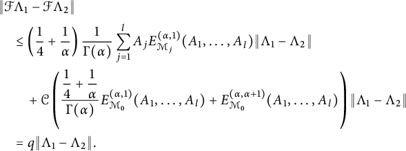 $$ \begin{align*} & {\left\lVert{\mathcal F \Lambda_1 - \mathcal F \Lambda_2}\right\rVert} \\& \quad \leq \left(\frac{1}{4} + \frac{1}{\alpha} \right) \frac{1}{\Gamma(\alpha)}\sum_{j = 1}^l A_j E_{\mathcal M_j}^{(\alpha, 1 )}(A_1, \dots, A_l) {\left\lVert{\Lambda_1 - \Lambda_2}\right\rVert} \\& \qquad + \mathcal C \left(\frac{\displaystyle \frac{1}{4} + \frac{1}{\alpha}}{\Gamma(\alpha)} E_{\mathcal M_0}^{(\alpha, 1 )}(A_1, \dots, A_l) + E_{\mathcal M_0}^{(\alpha, \alpha + 1 )}(A_1, \dots, A_l)\right) {\left\lVert{\Lambda_1 - \Lambda_2}\right\rVert} \\& \quad = q {\left\lVert{\Lambda_1 - \Lambda_2}\right\rVert}. \end{align*} $$
Since $q < 1$
, equation (1.1) has a unique uniformly bounded solution in
$q < 1$
, equation (1.1) has a unique uniformly bounded solution in $S([0, 1] \times [0, 1]^n)$
by BCP. The proof is completed.
$S([0, 1] \times [0, 1]^n)$
by BCP. The proof is completed.
3 The Hyers–Ulam stability
In this section, we are going to derive the Hyers–Ulam stability of equation (1.1) using the implicit integral equation from Section 2.
Definition 3.1 We say that the FNPIDE (1.1) is Hyers–Ulam stable if there exists a constant $\mathcal K> 0$
such that for all
$\mathcal K> 0$
such that for all $\epsilon> 0$
and a continuously differentiable function
$\epsilon> 0$
and a continuously differentiable function $\Lambda $
satisfying the three boundary conditions and the inequality
$\Lambda $
satisfying the three boundary conditions and the inequality
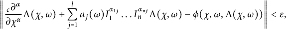 $$\begin{align*}{\left\lVert{\displaystyle \frac{ _c \partial^{\alpha}}{\partial \chi^{\alpha}} \Lambda(\chi, \omega) + \sum_{j = 1}^l a_j(\omega) I_1^{\alpha_{1 j}}\dots I_n^{\alpha_{n j}} \Lambda(\chi, \omega) - \phi(\chi, \omega, \Lambda(\chi, \omega))}\right\rVert} < \epsilon, \end{align*}$$
then there exists a solution $\Lambda _0$
of equation (1.1) such that
$\Lambda _0$
of equation (1.1) such that
 $$\begin{align*}{\left\lVert{\Lambda(\chi, \omega) - \Lambda_0(\chi, \omega) }\right\rVert} < \mathcal K \epsilon, \end{align*}$$
where $\mathcal K$
is a Hyers–Ulam stability constant.
$\mathcal K$
is a Hyers–Ulam stability constant.
Theorem 3.1 Suppose $a_j, \phi _1, \phi _2, \phi _3 \in C([0, 1]^n)$
for
$a_j, \phi _1, \phi _2, \phi _3 \in C([0, 1]^n)$
for $j = 1, 2, \dots , j$
,
$j = 1, 2, \dots , j$
, $\phi $
is a continuous function on
$\phi $
is a continuous function on $[0, 1] \times [0, 1]^n \times \mathbb R$
satisfying the Lipschitz condition for a positive constant
$[0, 1] \times [0, 1]^n \times \mathbb R$
satisfying the Lipschitz condition for a positive constant $\mathcal C$
 $$\begin{align*}| \phi (\chi, \omega, y_1) - \phi (\chi, \omega, y_2) | \leq \mathcal C |y_1 - y_2|, \;\; y_1, y_2 \in \mathbb R, \end{align*}$$ $\alpha _{ij} \geq 0 $
for all
$\alpha _{ij} \geq 0 $
for all $i = 1, \dots , n, \, j = 1, \dots , l$
, and there is
$i = 1, \dots , n, \, j = 1, \dots , l$
, and there is $1 \leq i_0 \leq n$
such that
$1 \leq i_0 \leq n$
such that $\alpha _{i_0 j}> 0$
for all
$\alpha _{i_0 j}> 0$
for all $j = 1, \dots , l$
. Furthermore, we assume that
$j = 1, \dots , l$
. Furthermore, we assume that
 $$ \begin{align*} \mathcal M_j = \begin{bmatrix} \alpha_{11} \dots & \alpha_{1l} & \alpha_{1 j}+ 1 \\ \alpha_{21} \dots & \alpha_{2l} & \alpha_{2 j} + 1\\ \dots & & \\ \alpha_{n1} \dots & \alpha_{n l} & \alpha_{n j } + 1 \\ \end{bmatrix}, \end{align*} $$
and
 $$ \begin{align*} q &= \left(\frac{1}{4} + \frac{1}{\alpha} \right) \frac{1}{\Gamma(\alpha)}\sum_{j = 1}^l A_j E_{\mathcal M_j}^{(\alpha, 1 )}(A_1, \dots, A_l) \\ & \quad + \mathcal C \left(\frac{\displaystyle \frac{1}{4} + \frac{1}{\alpha}}{\Gamma(\alpha)} E_{\mathcal M_0}^{(\alpha, 1 )}(A_1, \dots, A_l) + E_{\mathcal M_0}^{(\alpha, \alpha + 1 )}(A_1, \dots, A_l)\right) < 1, \end{align*} $$
where
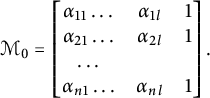 $$ \begin{align*} \mathcal M_0 = \begin{bmatrix} \alpha_{11} \dots & \alpha_{1l} & 1 \\ \alpha_{21} \dots & \alpha_{2l} & 1\\ \dots & & \\ \alpha_{n1} \dots & \alpha_{n l} & 1 \\ \end{bmatrix}. \end{align*} $$
Then equation (1.1) is Hyers–Ulam stable in the space $S([0, 1] \times [0, 1]^n).$
Proof Let
 $$\begin{align*}\Lambda_1(\chi, \omega) = \frac{ _c \partial^{\alpha}}{\partial \chi^{\alpha}} \Lambda(\chi, \omega) + \sum_{j = 1}^l a_j(\omega) I_1^{\alpha_{1 j}}\dots I_n^{\alpha_{n j}} \Lambda(\chi, \omega) - \phi(\chi, \omega, \Lambda(\chi, \omega)). \end{align*}$$
Then
 $$\begin{align*}\frac{ _c \partial^{\alpha}}{\partial \chi^{\alpha}} \Lambda(\chi, \omega) + \sum_{j = 1}^l a_j(\omega) I_1^{\alpha_{1 j}}\dots I_n^{\alpha_{n j}} \Lambda(\chi, \omega) = \phi(\chi, \omega, \Lambda(\chi, \omega)) + \Lambda_1(\chi, \omega), \end{align*}$$
and from our assumption
 $$\begin{align*}{\left\lVert{\Lambda_1}\right\rVert} < \epsilon. \end{align*}$$
It follows from the proof of Theorem 2.1 that
 $$ \begin{align*} & \Lambda(\chi, \omega) \\& \quad = \sum_{k = 0}^\infty (-1)^k \sum_{k_1 + \cdots + k_l = k} \binom{k}{k_1, \dots, k_l}\left(a_1 (\omega) I_\chi^{\alpha} I_1^{\alpha_{1 1}}\dots I_n^{\alpha_{n 1}}\right)^{k_1}\cdots \left( a_l (\omega) I_\chi^{\alpha} I_1^{\alpha_{1 l}}\dots I_n^{\alpha_{n l}}\right)^{k_l} \nonumber \\& \qquad \cdot ( \phi_1 (\omega) (1- 2 \chi + \chi^2) + \phi_2 (\omega) (2 \chi - \chi^2 ) + \phi_3 (\omega) (\chi^2 - \chi) + I_{\chi = 1}^{\alpha - 1} (\chi \phi - \chi^2 \phi) \nonumber \\& \qquad + I_{\chi = 1}^{\alpha} (\chi^2 \phi - 2 \chi \phi) + I_\chi^{\alpha} \phi + \sum_{j = 1}^l a_j(\omega) I_1^{\alpha_{1 j}}\dots I_n^{\alpha_{n j}} I_{\chi = 1}^{\alpha - 1} (\chi \Lambda - \chi^2 \Lambda) \nonumber \\& \qquad + \sum_{j = 1}^l a_j(\omega) I_1^{\alpha_{1 j}}\dots I_n^{\alpha_{n j}} I_{\chi = 1}^{\alpha } (\chi^2 \Lambda - 2 \chi \Lambda) \\& \qquad + I_{\chi = 1}^{\alpha - 1} (\chi \Lambda_1 - \chi^2 \Lambda_1) + I_{\chi = 1}^{\alpha} (\chi^2 \Lambda_1 - 2 \chi \Lambda_1) + I_\chi^{\alpha} \Lambda_1 ), \end{align*} $$
and
 $$ \begin{align*} & \Lambda_0(\chi, \omega) \\& \quad = \sum_{k = 0}^\infty (-1)^k \sum_{k_1 + \cdots + k_l = k} \binom{k}{k_1, \dots, k_l}\left(a_1 (\omega) I_\chi^{\alpha} I_1^{\alpha_{1 1}}\dots I_n^{\alpha_{n 1}}\right)^{k_1}\cdots \left( a_l (\omega) I_\chi^{\alpha} I_1^{\alpha_{1 l}}\dots I_n^{\alpha_{n l}}\right)^{k_l} \nonumber \\& \qquad \cdot ( \phi_1 (\omega) (1- 2 \chi + \chi^2) + \phi_2 (\omega) (2 \chi - \chi^2 ) + \phi_3 (\omega) (\chi^2 - \chi) + I_{\chi = 1}^{\alpha - 1} (\chi \phi - \chi^2 \phi) \nonumber \\& \qquad + I_{\chi = 1}^{\alpha} (\chi^2 \phi - 2 \chi \phi) + I_\chi^{\alpha} \phi + \sum_{j = 1}^l a_j(\omega) I_1^{\alpha_{1 j}}\dots I_n^{\alpha_{n j}} I_{\chi = 1}^{\alpha - 1} (\chi \Lambda_0 - \chi^2 \Lambda_0) \nonumber \\& \qquad + \sum_{j = 1}^l a_j(\omega) I_1^{\alpha_{1 j}}\dots I_n^{\alpha_{n j}} I_{\chi = 1}^{\alpha } (\chi^2 \Lambda_0 - 2 \chi \Lambda_0)), \end{align*} $$
by noting that $\phi $
is a continuous and
$\phi $
is a continuous and
 $$ \begin{align*} &\quad\kern1pt \sup_{(\chi, \omega) \in [0, 1] \times [0, 1]^n} |\phi(\chi, \omega, \Lambda(\chi, \omega))| \\ & \quad = \sup_{(\chi, \omega) \in [0, 1] \times [0, 1]^n} |\phi(\chi, \omega, \Lambda(\chi, \omega)) - \phi(\chi, \omega, 0) + \phi(\chi, \omega, 0) | \\ & \quad \leq \mathcal C {\left\lVert{\Lambda}\right\rVert} + \sup_{(\chi, \omega) \in [0, 1] \times [0, 1]^n} |\phi(\chi, \omega, 0)| < + \infty, \end{align*} $$
if $\Lambda \in S([0, 1] \times [0, 1]^n).$
Hence,
 $$ \begin{align*} & | \Lambda(\chi, \omega) - \Lambda_0 (\chi, \omega) | \\& \quad \leq \sum_{k = 0}^\infty \sum_{k_1 + \cdots + k_l = k} \binom{k}{k_1, \dots, k_l} A_1^{k_1} \dots A_l^{k_l} I_\chi^{\alpha k } I_1^{\alpha_{11} k_1 + \cdots + \alpha_{1 l} k_l} \\& \qquad \dots I_n^{\alpha_{n 1} k_1 + \cdots + \alpha_{nl} k_l} \cdot ( I_{\chi = 1}^{\alpha - 1} |(\chi - \chi^2)(\phi(\chi, \omega, \Lambda) - \phi(\chi, \omega, \Lambda_0))| \\& \qquad + I_{\chi = 1}^{\alpha} |(\chi^2 - 2 \chi ) (\phi(\chi, \omega, \Lambda) - \phi(\chi, \omega, \Lambda_0))| + I_\chi^{\alpha} |( \phi(\chi, \omega, \Lambda) - \phi(\chi, \omega, \Lambda_0) )| \\& \qquad+ \sum_{j = 1}^l a_j(\omega) I_1^{\alpha_{1 j}}\dots I_n^{\alpha_{n j}} I_{\chi = 1}^{\alpha - 1} |(\chi - \chi^2 ) (\Lambda - \Lambda_0 )| \\& \qquad + \sum_{j = 1}^l a_j(\omega) I_1^{\alpha_{1 j}}\dots I_n^{\alpha_{n j}} I_{\chi = 1}^{\alpha } | (\chi^2 - 2 \chi ) (\Lambda - \Lambda_0 ) | \\& \qquad + I_{\chi = 1}^{\alpha - 1} |(\chi \Lambda_1 - \chi^2 \Lambda_1)| + I_{\chi = 1}^{\alpha} |(\chi^2 \Lambda_1 - 2 \chi \Lambda_1)| + I_\chi^{\alpha} | \Lambda_1 | ), \end{align*} $$
which implies that
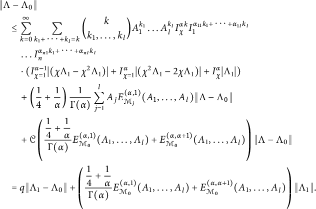 $$ \begin{align*} & {\left\lVert{ \Lambda - \Lambda_0 }\right\rVert} \\& \quad \leq \sum_{k = 0}^\infty \sum_{k_1 + \cdots + k_l = k} \binom{k}{k_1, \dots, k_l} A_1^{k_1} \dots A_l^{k_l} I_\chi^{\alpha k } I_1^{\alpha_{11} k_1 + \cdots + \alpha_{1 l} k_l} \\& \qquad \dots I_n^{\alpha_{n 1} k_1 + \cdots + \alpha_{nl} k_l} \\& \qquad \cdot ( I_{\chi = 1}^{\alpha - 1} |(\chi \Lambda_1 - \chi^2 \Lambda_1)| + I_{\chi = 1}^{\alpha} |(\chi^2 \Lambda_1 - 2 \chi \Lambda_1)| + I_\chi^{\alpha} | \Lambda_1 | ) \\& \qquad + \left(\frac{1}{4} + \frac{1}{\alpha} \right) \frac{1}{\Gamma(\alpha)}\sum_{j = 1}^l A_j E_{\mathcal M_j}^{(\alpha, 1 )}(A_1, \dots, A_l) {\left\lVert{\Lambda - \Lambda_0}\right\rVert} \\& \qquad + \mathcal C \left(\frac{\displaystyle \frac{1}{4} + \frac{1}{\alpha}}{\Gamma(\alpha)} E_{\mathcal M_0}^{(\alpha, 1 )}(A_1, \dots, A_l) + E_{\mathcal M_0}^{(\alpha, \alpha + 1 )}(A_1, \dots, A_l)\right) {\left\lVert{\Lambda - \Lambda_0}\right\rVert} \\& \quad = q {\left\lVert{\Lambda_1 - \Lambda_0}\right\rVert} + \left(\frac{\displaystyle \frac{1}{4} + \frac{1}{\alpha}}{\Gamma(\alpha)} E_{\mathcal M_0}^{(\alpha, 1 )}(A_1, \dots, A_l) + E_{\mathcal M_0}^{(\alpha, \alpha + 1 )}(A_1, \dots, A_l)\right) {\left\lVert{\Lambda_1}\right\rVert}. \end{align*} $$
Finally, we have
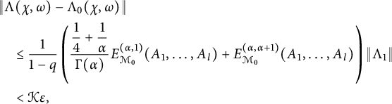 $$ \begin{align*} & {\left\lVert{ \Lambda(\chi, \omega) - \Lambda_0 (\chi, \omega) }\right\rVert} \\& \quad \leq \frac{1}{1 - q } \left(\frac{\displaystyle \frac{1}{4} + \frac{1}{\alpha}}{\Gamma(\alpha)} E_{\mathcal M_0}^{(\alpha, 1 )}(A_1, \dots, A_l) + E_{\mathcal M_0}^{(\alpha, \alpha + 1 )}(A_1, \dots, A_l)\right) {\left\lVert{\Lambda_1}\right\rVert} \\& \quad < \mathcal K \epsilon, \end{align*} $$
where
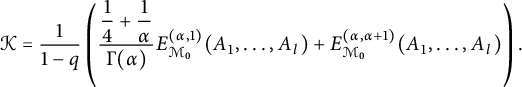 $$\begin{align*}\mathcal K = \frac{1}{1 - q } \left(\frac{\displaystyle \frac{1}{4} + \frac{1}{\alpha}}{\Gamma(\alpha)} E_{\mathcal M_0}^{(\alpha, 1 )}(A_1, \dots, A_l) + E_{\mathcal M_0}^{(\alpha, \alpha + 1 )}(A_1, \dots, A_l)\right). \end{align*}$$
This completes the proof.
Remark 3.2 We should point out that Theorem 3.1 does not require the condition that $\phi $
is a bounded function. Moreover,
$\phi $
is a bounded function. Moreover, $\Lambda _0$
is not a uniformly bounded function in general, which is different from Theorem 2.2. Since
$\Lambda _0$
is not a uniformly bounded function in general, which is different from Theorem 2.2. Since $\Omega = [0, 1] \times [0, 1]^n$
is bounded and closed (compact) the Hyers–Ulam stability is guaranteed by noting the fact that all continuous functions reach their maximum and minimum over
$\Omega = [0, 1] \times [0, 1]^n$
is bounded and closed (compact) the Hyers–Ulam stability is guaranteed by noting the fact that all continuous functions reach their maximum and minimum over $\Omega $
. The Hyers–Ulam stability constant
$\Omega $
. The Hyers–Ulam stability constant $\mathcal K$
obtained above is the best possible in our approach. There is a possible lower bound on the Hyers–Ulam stability constant but it would be tough and difficult to find it.
$\mathcal K$
obtained above is the best possible in our approach. There is a possible lower bound on the Hyers–Ulam stability constant but it would be tough and difficult to find it.
4 Examples
We will present two examples demonstrating applications of key theorems obtained from previous sections.
Example 4.1 The following fractional differential equation with a nonlocal initial condition:
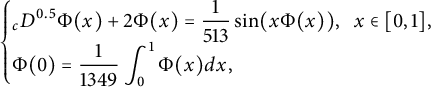 $$ \begin{align} \begin{cases} \displaystyle _c D^{0.5} \Phi (x) + 2 \Phi(x) = \frac{1}{513} \sin (x \Phi(x)), \;\; x \in [0, 1], \\ \Phi(0) = \displaystyle \frac{1}{1349} \int_0^1 \Phi(x) d x, \end{cases} \end{align} $$
has a unique solution in $C[0, 1]$
.
$C[0, 1]$
.
Proof Clearly,
 $$\begin{align*}f(x, y) = \frac{1}{513} \sin (x y) \end{align*}$$
is bounded and
 $$\begin{align*}| f(x, y_1) - f(x, y_2) | \leq \frac{1}{513} | x y_1 - x y_2| \leq \frac{1}{513} |y_1 - y_2|, \end{align*}$$
if $x \in [0, 1]$
. It remains to find the value
$x \in [0, 1]$
. It remains to find the value
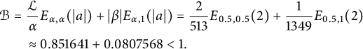 $$ \begin{align*} \mathcal B &= \frac{\mathcal L}{\alpha } E_{\alpha, \alpha }(|a|) + |\beta| E_{\alpha, 1}(|a|) = \frac{2}{513} E_{0.5, 0.5} (2) + \frac{1}{1349} E_{0.5, 1} (2) \\& \quad \approx 0.851641 + 0.0807568 < 1. \end{align*} $$
Hence, equation (4.1) has a unique solution in the Banach space $C[0, 1]$
.
$C[0, 1]$
.
Example 4.2 The following FNPIDE with a mixed boundary condition:
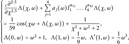 $$ \begin{align} \begin{cases} \displaystyle \frac{ _c \partial^{2.5}}{\partial \chi^{2.5}} \Lambda(\chi, \omega) + \sum_{j = 1}^4 a_j(\omega) I_1^{\alpha_{1 j}}\dots I_4^{\alpha_{4 j}} \Lambda(\chi, \omega) \\= \displaystyle \frac{1}{59} \cos(\chi \omega + \Lambda(\chi, \omega)) + \displaystyle \frac{1}{\chi^2 + \omega^2 + 2}, \\ \Lambda(0, \omega) = \omega^2 + 1, \;\; \Lambda(1, \omega) = \displaystyle \frac{1}{9} \omega, \,\, \Lambda'(1, \omega) = \displaystyle \frac{1}{6} \omega^3, \end{cases} \end{align} $$
where
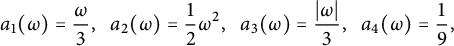 $$\begin{align*}a_1(\omega) = \frac{\omega}{3}, \;\; a_2(\omega) = \frac{1}{2} \omega^2, \;\; a_3(\omega) = \frac{|\omega|}{3}, \;\; a_4(\omega) = \frac{1}{9}, \end{align*}$$
and
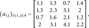 $$ \begin{align*} \mathcal (\alpha_{ij})_{1 \leq i, j \leq 4} = \begin{bmatrix} 1.1 & 1.3 & 0.7 & 1.4 \\ 1.3 & 2.3 & 3.1 & 2 \\ 0.7 & 1.6 & 2.1 & 1.2 \\ 2 & 3.1 & 4.1 & 2.2 \\ \end{bmatrix}, \end{align*} $$
has a unique uniformly bounded solution and the Hyers–Ulam stability in the space $S([0, 1] \times [0, 1]^4)$
.
$S([0, 1] \times [0, 1]^4)$
.
Proof Clearly, $a_j$
for
$a_j$
for $j = 1, 2, 3, 4$
,
$j = 1, 2, 3, 4$
, $\phi _1, \, \phi _2, \, \phi _3 \in C([0, 1]^4)$
and
$\phi _1, \, \phi _2, \, \phi _3 \in C([0, 1]^4)$
and
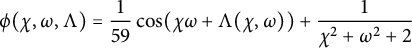 $$\begin{align*}\phi(\chi, \omega, \Lambda) = \frac{1}{59} \cos(\chi \omega + \Lambda(\chi, \omega)) + \displaystyle \frac{1}{\chi^2 + \omega^2 + 2} \end{align*}$$
is a continuous and bounded function on $[0, 1] \times [0, 1]^4 \times \mathbb R$
, satisfying the Lipschitz condition with
$[0, 1] \times [0, 1]^4 \times \mathbb R$
, satisfying the Lipschitz condition with $\mathcal C = 1/59$
:
$\mathcal C = 1/59$
:
 $$\begin{align*}| \phi(\chi, \omega, y_1) -\phi(\chi, \omega, y_2) | \leq \frac{1}{59} |\cos (\chi \omega + y_1) - \cos (\chi \omega + y_2) | \leq \frac{1}{59} |y_1 - y_2|. \end{align*}$$
Furthermore,
 $$\begin{align*}A_1 = 1/3, \;\; A_2 = 1/2, \;\; A_3 = 1/3, \;\; A_4 = 1/9. \end{align*}$$
We need to compute the value
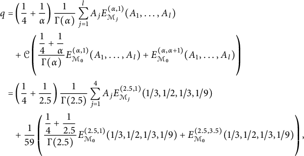 $$ \begin{align*} q = & \left(\frac{1}{4} + \frac{1}{\alpha} \right) \frac{1}{\Gamma(\alpha)}\sum_{j = 1}^l A_j E_{\mathcal M_j}^{(\alpha, 1 )}(A_1, \dots, A_l) \\ & + \mathcal C \left(\frac{\displaystyle \frac{1}{4} + \frac{1}{\alpha}}{\Gamma(\alpha)} E_{\mathcal M_0}^{(\alpha, 1 )}(A_1, \dots, A_l) + E_{\mathcal M_0}^{(\alpha, \alpha + 1 )}(A_1, \dots, A_l)\right) \\ = & \left(\frac{1}{4} + \frac{1}{2.5} \right) \frac{1}{\Gamma(2.5)}\sum_{j = 1}^4 A_j E_{\mathcal M_j}^{(2.5, 1 )}(1/3, 1/2, 1/3, 1/9) \\ & + \frac{1}{59} \left(\frac{\displaystyle \frac{1}{4} + \frac{1}{2.5}}{\Gamma(2.5)} E_{\mathcal M_0}^{(2.5, 1 )}(1/3, 1/2, 1/3, 1/9) + E_{\mathcal M_0}^{(2.5, 3.5 )}(1/3, 1/2, 1/3, 1/9)\right), \end{align*} $$
where
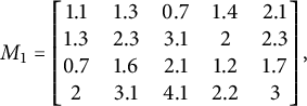 $$\begin{align*}M_1 = \begin{bmatrix} 1.1 & 1.3 & 0.7 & 1.4 & 2.1 \\ 1.3 & 2.3 & 3.1 & 2 & 2.3 \\ 0.7 & 1.6 & 2.1 & 1.2 & 1.7 \\ 2 & 3.1 & 4.1 & 2.2 & 3 \\ \end{bmatrix}, \end{align*}$$
 $$\begin{align*}M_2 = \begin{bmatrix} 1.1 & 1.3 & 0.7 & 1.4 & 2.3 \\ 1.3 & 2.3 & 3.1 & 2 & 3.3 \\ 0.7 & 1.6 & 2.1 & 1.2 & 2.6 \\ 2 & 3.1 & 4.1 & 2.2 & 4.1 \\ \end{bmatrix}, \end{align*}$$
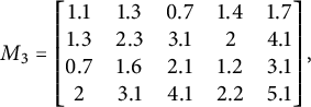 $$ \begin{align*} M_3 = \begin{bmatrix} 1.1 & 1.3 & 0.7 & 1.4 & 1.7 \\ 1.3 & 2.3 & 3.1 & 2 & 4.1 \\ 0.7 & 1.6 & 2.1 & 1.2 & 3.1 \\ 2 & 3.1 & 4.1 & 2.2 & 5.1 \\ \end{bmatrix}, \end{align*} $$
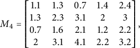 $$ \begin{align*} M_4 = \begin{bmatrix} 1.1 & 1.3 & 0.7 & 1.4 & 2.4\\ 1.3 & 2.3 & 3.1 & 2 & 3 \\ 0.7 & 1.6 & 2.1 & 1.2 & 2.2 \\ 2 & 3.1 & 4.1 & 2.2 & 3.2 \\ \end{bmatrix}, \end{align*} $$
and finally
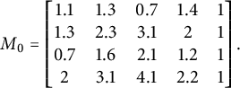 $$ \begin{align*} M_0 = \begin{bmatrix} 1.1 & 1.3 & 0.7 & 1.4 & 1 \\ 1.3 & 2.3 & 3.1 & 2 & 1 \\ 0.7 & 1.6 & 2.1 & 1.2 & 1 \\ 2 & 3.1 & 4.1 & 2.2 & 1 \\ \end{bmatrix}. \end{align*} $$
Using the following Python codes to get
 $$\begin{align*}q = 6.49406088226196* 10^{-293} < 1. \end{align*}$$
Hence, equation (4.2) has a unique uniformly bounded solution in the space $S([0, 1] \times [0, 1]^4)$
by Theorem 2.2, and it is Hyers–Ulam stable by Theorem 3.1.
$S([0, 1] \times [0, 1]^4)$
by Theorem 2.2, and it is Hyers–Ulam stable by Theorem 3.1.
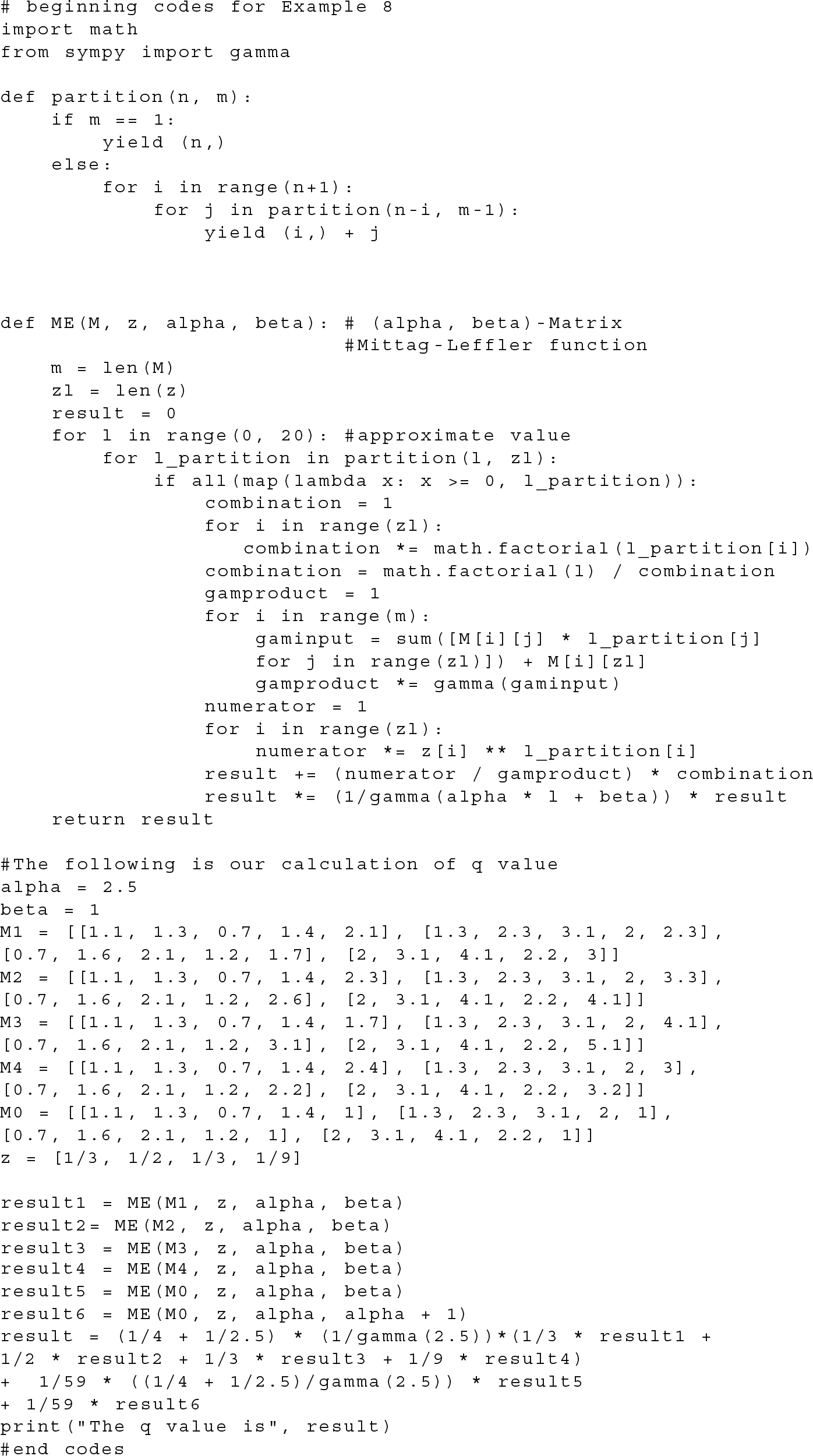
Remark 4.3 We have used the Python language to find approximates values of our newly established pair-parameter matrix Mittag–Leffler functions to study the uniqueness of solutions to equation (1.1). Slightly changing the codes we can compute values of the multivariate Mittag–Leffler functions. As far as we know from current research related to computation of the Mittag–Leffler functions, this approach is efficient and simple.
5 Conclusion
We have studied the uniqueness and Hyers–Ulam stability to the new equation (1.1) based on the pair-parameter matrix Mittag–Leffler functions, Banach’s contractive principle as well as Babenko’s approach. A few examples were provided to demonstrate applications of main results derived. The methods used in the current work are also suitable for different types of differential equations with various initial or boundary conditions, as well as integral equations with variable coefficients, which cannot be handled by any existing integral transforms.
Acknowledgments
The author is thankful to the reviewers and editor for giving valuable comments and suggestions.
Competing interests
The author declares no competing interests.
Data availability statement
No data were used to support this study.


 Open access