


1. Introduction
The Potts model, originally invented to study ferromagnetism [Reference Potts18], is a model from statistical physics; it also plays a central role in probability theory, combinatorics and computer science.
Let $G = (V,E)$
be a finite graph. The Potts model on the graph
$G = (V,E)$
be a finite graph. The Potts model on the graph $G$
has two parameters, a number of states
$G$
has two parameters, a number of states $q \in \mathbb{Z}_{\geq 2}$
and an interaction parameter
$q \in \mathbb{Z}_{\geq 2}$
and an interaction parameter $w\geq 0$
. The case
$w\geq 0$
. The case $q=2$
is known as the Ising model. A configuration is a map
$q=2$
is known as the Ising model. A configuration is a map $\sigma\;:\;V \to [q]\;:\!=\;\{1,\ldots,q\}$
. Associated with such a configuration is a weight
Footnote
1
$\sigma\;:\;V \to [q]\;:\!=\;\{1,\ldots,q\}$
. Associated with such a configuration is a weight
Footnote
1 $w^{m(\sigma )}$
, where
$w^{m(\sigma )}$
, where $m(\sigma )$
is the number of monochromatic edges in the configuration
$m(\sigma )$
is the number of monochromatic edges in the configuration $\sigma$
. The
$\sigma$
. The $q$
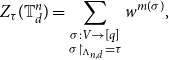
-state partition function of the Potts model is the sum of the weights over all configurations; we denote it as
$q$
-state partition function of the Potts model is the sum of the weights over all configurations; we denote it as $ Z(G, q, w) = \sum _{ \sigma:V \rightarrow [q]}\!w^{m(\sigma )}.$
In statistical physics one has
$ Z(G, q, w) = \sum _{ \sigma:V \rightarrow [q]}\!w^{m(\sigma )}.$
In statistical physics one has $w=e^{kJ/T}$
, with
$w=e^{kJ/T}$
, with $J$
being an interaction parameter,
$J$
being an interaction parameter, $k$
the Boltzmann constant and
$k$
the Boltzmann constant and $T$
the temperature. We write
$T$
the temperature. We write $Z(G)$
to keep notation short.
$Z(G)$
to keep notation short.
The Gibbs measure is the probability measure $\mathbb{P}_G[\cdot]$
on the set of configurations of
$\mathbb{P}_G[\cdot]$
on the set of configurations of $G=(V,E)$
, where the probability of a random configurationFootnote
2
$G=(V,E)$
, where the probability of a random configurationFootnote
2 $\boldsymbol{\Phi }$
being equal to a given configuration
$\boldsymbol{\Phi }$
being equal to a given configuration $\phi\;:\;V\to [q]$
is proportional to the weight of
$\phi\;:\;V\to [q]$
is proportional to the weight of $\phi$
:
$\phi$
:
 \begin{equation} \mathbb{P}_{G}[{\boldsymbol \Phi }=\phi ] = \frac{w^{m(\sigma )}}{Z(G)}. \end{equation}
The Potts model is said to be ferromagnetic if $w \gt 1$
and anti-ferromagnetic if
$w \gt 1$
and anti-ferromagnetic if $w \lt 1$
. The ferromagnetic Potts model favours configurations with a large number of monochromatic edges, while the anti-ferromagnetic Potts model favours configurations with a small number of monochromatic edges, i.e., configurations that are ‘close’ to proper colourings.
$w \lt 1$
. The ferromagnetic Potts model favours configurations with a large number of monochromatic edges, while the anti-ferromagnetic Potts model favours configurations with a small number of monochromatic edges, i.e., configurations that are ‘close’ to proper colourings.
In statistical physics, models like the Potts model are typically considered on infinite graphs such as $\mathbb{Z}^d$
or the Bethe lattice
$\mathbb{Z}^d$
or the Bethe lattice $\mathbb{T}_d$
, also known as the infinite
$\mathbb{T}_d$
, also known as the infinite $(d+1)$
-regular tree. One can extend the notion of Gibbs measures for finite graphs to this infinite setting (see below for more details). The Gibbs measure on a finite graph is clearly unique. For infinite graphs, depending on the underlying parameter
$(d+1)$
-regular tree. One can extend the notion of Gibbs measures for finite graphs to this infinite setting (see below for more details). The Gibbs measure on a finite graph is clearly unique. For infinite graphs, depending on the underlying parameter $w$
, there may however be multiple Gibbs measures. The transition from having a unique Gibbs measure to multiple Gibbs measures is referred to as a phase transition in statistical physics [Reference Friedli and Velenik10] and it is an important problem to determine when this happens in terms of the underlying parameters of the model. Moreover, for several
$w$
, there may however be multiple Gibbs measures. The transition from having a unique Gibbs measure to multiple Gibbs measures is referred to as a phase transition in statistical physics [Reference Friedli and Velenik10] and it is an important problem to determine when this happens in terms of the underlying parameters of the model. Moreover, for several $2$
-state models, the uniqueness region and the transition from uniqueness to non-uniqueness of the Gibbs measure on
$2$
-state models, the uniqueness region and the transition from uniqueness to non-uniqueness of the Gibbs measure on $\mathbb{T}_d$
have been connected to the tractability of approximately computing partition functions of these models. See e.g. [Reference Weitz24, Reference Sly21, Reference Sly and Sun22, Reference Galanis, Štefankovič and Vigoda13, Reference Sinclair, Srivastava and Thurley23, Reference Li, Lu and Yin15]. In the case of the anti-ferromagnetic Potts model it is known that in the uniqueness regime on
$\mathbb{T}_d$
have been connected to the tractability of approximately computing partition functions of these models. See e.g. [Reference Weitz24, Reference Sly21, Reference Sly and Sun22, Reference Galanis, Štefankovič and Vigoda13, Reference Sinclair, Srivastava and Thurley23, Reference Li, Lu and Yin15]. In the case of the anti-ferromagnetic Potts model it is known that in the uniqueness regime on $\mathbb{T}_d$
there is an efficient algorithm to approximately compute the partition function and sample from the Gibbs measure on random
$\mathbb{T}_d$
there is an efficient algorithm to approximately compute the partition function and sample from the Gibbs measure on random $(d+1)$
-regular graphs [Reference Blanca, Galanis, Goldberg, Štefankovič, Vigoda and Yang4]. See also [Reference Efthymiou9] for related results on Erdős-Rényi random graphs without any assumption on uniqueness. It is moreover expected that the uniqueness to non-uniqueness transition for the anti-ferromagnetic Potts model says something about the tractability of approximating the partition function for the entire class of bounded degree graphs. In particular, approximating the partition function of the Potts model is NP-hard on graphs of maximum degree
$(d+1)$
-regular graphs [Reference Blanca, Galanis, Goldberg, Štefankovič, Vigoda and Yang4]. See also [Reference Efthymiou9] for related results on Erdős-Rényi random graphs without any assumption on uniqueness. It is moreover expected that the uniqueness to non-uniqueness transition for the anti-ferromagnetic Potts model says something about the tractability of approximating the partition function for the entire class of bounded degree graphs. In particular, approximating the partition function of the Potts model is NP-hard on graphs of maximum degree $d+1$
when
$d+1$
when $0\lt w\lt 1 - \frac{q}{d+1}$
[Reference Galanis, Štefankovič and Vigoda12] (for even
$0\lt w\lt 1 - \frac{q}{d+1}$
[Reference Galanis, Štefankovič and Vigoda12] (for even $q$
). It is a major open problem to determine whether there exist efficient algorithms for all
$q$
). It is a major open problem to determine whether there exist efficient algorithms for all $w\in (1-\frac{q}{d+1},1]$
.
$w\in (1-\frac{q}{d+1},1]$
.
In the present paper we consider the problem of determining when the anti-ferromagnetic Potts model on the infinite $(d+1)$
-regular tree has a unique Gibbs measure. Before stating our main result, we first give a formal definition of Gibbs measures on the
$(d+1)$
-regular tree has a unique Gibbs measure. Before stating our main result, we first give a formal definition of Gibbs measures on the $(d+1)$
-regular tree.
$(d+1)$
-regular tree.
Gibbs measures, uniqueness and main result
We follow Brightwell and Winkler [Reference Brightwell and Winkler7, Reference Brightwell and Winkler8] to introduce the notion of Gibbs measures on $\mathbb{T}_d$
, see also [Reference Rozikov20, Reference Friedli and Velenik10] for more details and background.
$\mathbb{T}_d$
, see also [Reference Rozikov20, Reference Friedli and Velenik10] for more details and background.
Throughout we fix a degree $d\geq 2$
and an integer
$d\geq 2$
and an integer $q\geq 2$
. We denote the vertex set of
$q\geq 2$
. We denote the vertex set of $\mathbb{T}_d$
by
$\mathbb{T}_d$
by $V_d$
and we denote the space of all configurations
$V_d$
and we denote the space of all configurations $\{\psi\;:\;V_d\to [q]\}$
by
$\{\psi\;:\;V_d\to [q]\}$
by $\Omega _{q,d}$
. For a set
$\Omega _{q,d}$
. For a set $U\subset V_d$
we denote by
$U\subset V_d$
we denote by $\partial U$
the set of vertices in
$\partial U$
the set of vertices in $U$
that are adjacent to some vertex in
$U$
that are adjacent to some vertex in $V_d\setminus U$
. We refer to
$V_d\setminus U$
. We refer to $\partial U$
as the boundary of
$\partial U$
as the boundary of $U$
. We denote by
$U$
. We denote by $U^{\circ }\;:\!=\;U\setminus \partial U$
the interior of
$U^{\circ }\;:\!=\;U\setminus \partial U$
the interior of $U$
. For
$U$
. For $\psi \in \Omega _{q,d}$
and
$\psi \in \Omega _{q,d}$
and $U\subset V_d$
we denote the restriction of
$U\subset V_d$
we denote the restriction of $\psi$
to
$\psi$
to $U$
by
$U$
by $\psi \!\restriction _U$
.
$\psi \!\restriction _U$
.
Definition 1.1. (Gibbs measure) We equip $\Omega _{q,d}$
with the sigma algebra generated by sets of the form
$\Omega _{q,d}$
with the sigma algebra generated by sets of the form $\{\psi \in \Omega _{q,d}\mid \psi \!\restriction _U=\phi \}$
where
$\{\psi \in \Omega _{q,d}\mid \psi \!\restriction _U=\phi \}$
where $U\subset V_d$
is a finite set and
$U\subset V_d$
is a finite set and $\phi\;:\;U\to [q]$
a fixed colouring of
$\phi\;:\;U\to [q]$
a fixed colouring of $U$
. A probability measure
$U$
. A probability measure $\mu$
on
$\mu$
on $\Omega _{q,d}$
is called a Gibbs measure if for any finite set
$\Omega _{q,d}$
is called a Gibbs measure if for any finite set $U\subset V_d$
and
$U\subset V_d$
and $\mu$
-almost every
$\mu$
-almost every $\phi \in \Omega _{q,d}$
, we have
$\phi \in \Omega _{q,d}$
, we have
 \begin{equation} \mathbb{P}_{{\boldsymbol \Phi }\sim \mu }[{\boldsymbol \Phi }\!\restriction _{U}=\phi \!\restriction _{U} \mid{{\boldsymbol \Phi }}\!\restriction _{V_d\setminus U^{\circ }} = \phi \!\restriction _{V_d\setminus U^\circ }\!]= \mathbb{P}_{U}[{\boldsymbol \Phi }\!\restriction _{U} = \phi \!\restriction _U \big |{\boldsymbol \Phi }\!\restriction _{\partial U} = \phi \!\restriction _{\partial U}\!], \end{equation}
where the second probability $\mathbb{P}_{U}$
denotes the probability of seeing configuration
$\mathbb{P}_{U}$
denotes the probability of seeing configuration $\phi$
on the finite graph
$\phi$
on the finite graph $\mathbb{T}_d[U]$
induced by
$\mathbb{T}_d[U]$
induced by $U$
conditioned on the event of being equal to
$U$
conditioned on the event of being equal to $\phi$
on
$\phi$
on $\partial U$
. This latter probability is obtained by dividing the weight of
$\partial U$
. This latter probability is obtained by dividing the weight of ${\boldsymbol \Phi }\!\restriction _U$
by the sum of the weights of all colourings of
${\boldsymbol \Phi }\!\restriction _U$
by the sum of the weights of all colourings of $U$
that agree with
$U$
that agree with $\phi$
on
$\phi$
on $\partial U$
, cf. (1).
$\partial U$
, cf. (1).
Remark 1.2. Note that the conditional probability on the left-hand side of (2) cannot be computed using the standard formula for conditional probabilities, as we in general condition on an event of measure zero. Therefore, the formalism of conditional expectations should be used to evaluate this conditional probability. See [Reference Friedli and Velenik10] for more details.
By a compactness argument one can show that there always is at least one Gibbs measure on $\Omega _{q,d}$
cf. [Reference Friedli and Velenik10, Reference Brightwell and Winkler7]. The question of whether there is a unique Gibbs measure can be reformulated in terms of a certain decay of correlations. To do so we require some definitions. We denote by
$\Omega _{q,d}$
cf. [Reference Friedli and Velenik10, Reference Brightwell and Winkler7]. The question of whether there is a unique Gibbs measure can be reformulated in terms of a certain decay of correlations. To do so we require some definitions. We denote by $\mathbb{T}^n_{d}$
the finite tree obtained from
$\mathbb{T}^n_{d}$
the finite tree obtained from $\mathbb{T}_d$
by fixing a root vertex
$\mathbb{T}_d$
by fixing a root vertex $r_d$
, deleting all vertices at distance more than
$r_d$
, deleting all vertices at distance more than $n$
from the root, deleting one of the neighbours of
$n$
from the root, deleting one of the neighbours of $r_d$
and keeping the connected component containing
$r_d$
and keeping the connected component containing $r_d$
. We denote the set of leaves of
$r_d$
. We denote the set of leaves of $\mathbb{T}^n_{d}$
by
$\mathbb{T}^n_{d}$
by $\Lambda _{n,d}$
, except when
$\Lambda _{n,d}$
, except when $n=0$
, in which case we let
$n=0$
, in which case we let $\Lambda _{d,0}=\{r_d\}$
. We omit the reference to
$\Lambda _{d,0}=\{r_d\}$
. We omit the reference to $d$
when this is clear from the context. The next lemma reformulates uniqueness of the Gibbs measure in terms of the dependence on the distribution of the colours of the root vertex on the colouring of the leaves.
$d$
when this is clear from the context. The next lemma reformulates uniqueness of the Gibbs measure in terms of the dependence on the distribution of the colours of the root vertex on the colouring of the leaves.
Lemma 1.3.
The $q$
-state Potts model with parameter
$q$
-state Potts model with parameter $w\geq 0$
on the infinite
$w\geq 0$
on the infinite $(d+1)$
-regular tree has a unique Gibbs measure if and only if for all colours
$(d+1)$
-regular tree has a unique Gibbs measure if and only if for all colours $c \in [q]$
it holds that
$c \in [q]$
it holds that
 \begin{equation} \limsup _{n \to \infty } \max _{\tau:\Lambda _{n,d} \to [q]} \bigg \vert \mathbb{P}_{\mathbb{T}^n_{d}} [{\boldsymbol \Phi }(r_d) = c \vert{\boldsymbol \Phi }\!\restriction _{ \Lambda _{n,d}} = \tau ] - \frac{1}{q}\bigg \vert = 0. \end{equation}
While this result is well known we will provide a proof for convenience of the reader in Appendix A based on Brightwel and Winkler’s proof [Reference Brightwell and Winkler8, Theorem 3.3] for the case $w=0$
. We moreover note that (3) is the property of uniqueness used in algorithmic applications [Reference Blanca, Galanis, Goldberg, Štefankovič, Vigoda and Yang4].
$w=0$
. We moreover note that (3) is the property of uniqueness used in algorithmic applications [Reference Blanca, Galanis, Goldberg, Štefankovič, Vigoda and Yang4].
Define $w_c\;:\!=\;\max \{0,1-\frac{q}{d+1}\}$
. It is a folklore conjecture that this Gibbs measure is unique if and only if
$w_c\;:\!=\;\max \{0,1-\frac{q}{d+1}\}$
. It is a folklore conjecture that this Gibbs measure is unique if and only if $w\geq w_c$
(if
$w\geq w_c$
(if $q=d+1$
, the inequality should be read as a strict inequality). Non-uniqueness for
$q=d+1$
, the inequality should be read as a strict inequality). Non-uniqueness for $w\lt w_c$
has been known for a long time [Reference Peruggi, di Liberto and Monroy17, Reference Peruggi, di Liberto and Monroy16]
$w\lt w_c$
has been known for a long time [Reference Peruggi, di Liberto and Monroy17, Reference Peruggi, di Liberto and Monroy16]
For $q\gt d+1$
and thus
$q\gt d+1$
and thus $w_c=0$
, a Gibbs measure is supported on proper
$w_c=0$
, a Gibbs measure is supported on proper $q$
-colourings and in this case the conjecture has been shown to be true by Jonasson [Reference Jonasson14]. For the case
$q$
-colourings and in this case the conjecture has been shown to be true by Jonasson [Reference Jonasson14]. For the case $q=3$
and
$q=3$
and $d\geq 2$
and the case
$d\geq 2$
and the case $q=4$
and
$q=4$
and $d=4$
this has recently been proved by Galanis, Goldberg and Yang [Reference Galanis, Goldberg and Yang11]. Our main result confirms this conjecture for
$d=4$
this has recently been proved by Galanis, Goldberg and Yang [Reference Galanis, Goldberg and Yang11]. Our main result confirms this conjecture for $q=4$
and
$q=4$
and $d\geq 4$
. Very recently Bencs together with the authors of the present paper [Reference Bencs, de Boer, Buys and Regts2] have confirmed this conjecture for all
$d\geq 4$
. Very recently Bencs together with the authors of the present paper [Reference Bencs, de Boer, Buys and Regts2] have confirmed this conjecture for all $q\geq 5$
provided
$q\geq 5$
provided $d$
is large enough.
$d$
is large enough.
Main Theorem.
Let $d\in \mathbb{N}_{\geq 4}$
. Then the
$d\in \mathbb{N}_{\geq 4}$
. Then the $4$
-state anti-ferromagnetic Potts model on
$4$
-state anti-ferromagnetic Potts model on $\mathbb{T}_d$
has a unique Gibbs measure if and only if
$\mathbb{T}_d$
has a unique Gibbs measure if and only if $w\geq 1-\frac{4}{d+1}$
.
$w\geq 1-\frac{4}{d+1}$
.
Our proof of this result follows a different approach than the one taken in [Reference Galanis, Goldberg and Yang11], which heavily relies on rigorous (but not easily verifiable) computer calculations. In particular, our approach allows us to recover the results from [Reference Galanis, Goldberg and Yang11], thereby removing the need for these computer calculations. See Theorem 3.8 below for the full statement of what we prove with our approach.
Organization. In the next section we discuss our approach towards proving our main theorem arriving at a geometric condition for uniqueness that we check in Section 3 to prove our main theorem, deferring the verification of a crucial inequality to Section 4. Finally, in Section 5 we finish with some concluding remarks and open questions.
2. Approach and setup
Our main goal in this section is to derive a geometric condition for ratios of probabilities that implies uniqueness of the Gibbs measure on the $(d+1)$
-regular tree. This condition will then be verified in the following sections. Along the way we will comment on how our approach relates to the approach of Galanis, Goldberg and Yang [Reference Galanis, Goldberg and Yang11].
$(d+1)$
-regular tree. This condition will then be verified in the following sections. Along the way we will comment on how our approach relates to the approach of Galanis, Goldberg and Yang [Reference Galanis, Goldberg and Yang11].
2.1 Ratios of probabilities and the tree recursion
Instead of working directly with the probabilities we work with ratios of probabilities just as in [Reference Galanis, Goldberg and Yang11].
Let us introduce a few concepts to facilitate the discussion. Fix $n,d\in \mathbb{N}$
and write
$n,d\in \mathbb{N}$
and write $\mathbb{T}^n_{d}=(V,E)$
. Let
$\mathbb{T}^n_{d}=(V,E)$
. Let $\tau\;:\;\Lambda _{n,d}\to [q]$
. This will be called a boundary condition. We denote by
$\tau\;:\;\Lambda _{n,d}\to [q]$
. This will be called a boundary condition. We denote by
 \begin{equation} Z_{\tau }(\mathbb{T}^n_{d}) = \sum _{\substack{ \sigma:V \rightarrow [q]\\ \sigma \restriction _{\!\Lambda _{n,d}} = \tau }} w^{m(\sigma )}, \end{equation}
the restricted partition function. For $i \in [q]$
we denote by
$i \in [q]$
we denote by $Z_{i,\tau }(\mathbb{T}^n_{d})$
the sum (4) restricted to those
$Z_{i,\tau }(\mathbb{T}^n_{d})$
the sum (4) restricted to those $\sigma$
that associate colour
$\sigma$
that associate colour $i$
to the root vertex. We define the ratio
$i$
to the root vertex. We define the ratio
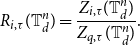 \begin{equation} R_{i,\tau }(\mathbb{T}^n_{d}) = \frac{Z_{i,\tau }(\mathbb{T}^n_{d})}{Z_{q,\tau }(\mathbb{T}^n_{d})}. \end{equation}
Note that $R_{q,\tau }(\mathbb{T}^n_{d})=1$
. We moreover remark that
$R_{q,\tau }(\mathbb{T}^n_{d})=1$
. We moreover remark that $R_{i,\tau }(\mathbb{T}^n_{d})$
can be interpreted as the ratio of the probabilities that the root gets colour
$R_{i,\tau }(\mathbb{T}^n_{d})$
can be interpreted as the ratio of the probabilities that the root gets colour $i$
(resp.
$i$
(resp. $q$
) given the boundary condition
$q$
) given the boundary condition $\tau$
.
$\tau$
.
We define for $n \geq 0$
,
$n \geq 0$
, $\widehat{\mathbb{T}}^n_{d}$
to be the rooted tree obtained from
$\widehat{\mathbb{T}}^n_{d}$
to be the rooted tree obtained from $\mathbb{T}^n_{d}$
by adding a new root
$\mathbb{T}^n_{d}$
by adding a new root $\hat r_d$
connecting it to the original root
$\hat r_d$
connecting it to the original root $r_d$
with a single edge. Note that the set of non-root leaves of
$r_d$
with a single edge. Note that the set of non-root leaves of $\widehat{\mathbb{T}}^n_{d}$
is just
$\widehat{\mathbb{T}}^n_{d}$
is just $\Lambda _{n,d}$
. For any boundary condition on
$\Lambda _{n,d}$
. For any boundary condition on $\tau\;:\;\Lambda _{n,d}\to [q]$
we define the restricted partition function,
$\tau\;:\;\Lambda _{n,d}\to [q]$
we define the restricted partition function, $Z_{i,\tau }(\widehat{\mathbb{T}}^n_{d})$
and ratio
$Z_{i,\tau }(\widehat{\mathbb{T}}^n_{d})$
and ratio $R_{i,\tau }(\widehat{\mathbb{T}}^n_{d})$
analogously as for
$R_{i,\tau }(\widehat{\mathbb{T}}^n_{d})$
analogously as for ${\mathbb{T}}^n_{d}$
.
${\mathbb{T}}^n_{d}$
.
The next lemma provides a sufficient condition for ${\mathbb{T}}_{d}$
to have a unique Gibbs measure in terms of these ratios, which we prove at the end of this section.
${\mathbb{T}}_{d}$
to have a unique Gibbs measure in terms of these ratios, which we prove at the end of this section.
Lemma 2.1.
Let $q,d \in \mathbb{N}$
and
$q,d \in \mathbb{N}$
and $w\in (0,1)$
. Suppose that for all
$w\in (0,1)$
. Suppose that for all $i \in [q-1]$
and for all
$i \in [q-1]$
and for all $\delta \gt 0$
there exists
$\delta \gt 0$
there exists $N \gt 0$
such that for all
$N \gt 0$
such that for all $n \geq N$
and for all boundary conditions
$n \geq N$
and for all boundary conditions $\tau\;:\;\Lambda _{n,d} \to [q]$
we have
$\tau\;:\;\Lambda _{n,d} \to [q]$
we have
 \begin{equation*} |R_{i,\tau }(\widehat {\mathbb {T}}^n_{d})-1| \lt \delta, \end{equation*}
then the tree ${\mathbb{T}}_{d}$
has a unique Gibbs measure.
${\mathbb{T}}_{d}$
has a unique Gibbs measure.
An advantage of working with the ratios of probabilities is that the well known tree recursion for the Potts model takes a convenient form.
Lemma 2.2.
Let $n,d\in \mathbb{N}$
and let
$n,d\in \mathbb{N}$
and let $\tau\;:\;\Lambda _{n,d}\to [q]$
be a boundary condition. Let for
$\tau\;:\;\Lambda _{n,d}\to [q]$
be a boundary condition. Let for $i=1,\ldots,d$
,
$i=1,\ldots,d$
, $T_i=\widehat{\mathbb{T}}^{n-1}_{d}$
be the components of
$T_i=\widehat{\mathbb{T}}^{n-1}_{d}$
be the components of $\mathbb{T}^n_d-r_d$
where we attach a new root vertex to
$\mathbb{T}^n_d-r_d$
where we attach a new root vertex to $r_{d-1}$
. Let
$r_{d-1}$
. Let $\tau _i$
be the restriction of
$\tau _i$
be the restriction of $\tau$
to
$\tau$
to $\Lambda _{n-1,d}\to [q]$
viewed as a subset of the vertices of
$\Lambda _{n-1,d}\to [q]$
viewed as a subset of the vertices of $T_i$
. Then we have for each
$T_i$
. Then we have for each $i \in [q-1],$
 \begin{equation} R_{i,\tau }(\widehat{\mathbb{T}}^{n}_{d}) = \frac{1++ w \prod _{s=1}^{d} R_{l,\tau _s}(\widehat{\mathbb{T}}^{n-1}_{d})+\sum _{l \in [q-1] \setminus \{i\}} \prod _{s=1}^{d} R_{l,\tau _s}(\widehat{\mathbb{T}}^{n-1}_{d}) }{w+\sum _{l \in [q-1] } \prod _{s=1}^{d} R_{l,\tau _s}(\widehat{\mathbb{T}}^{n-1}_{d})}. \end{equation}
For completeness we provide a proof for this lemma at the end of this section.
A direct analysis of the recursion in Lemma 2.2 is not straightforward, as it does not contract uniformly on a symmetric domain. In [Reference Galanis, Goldberg and Yang11] this is remedied by looking at the two-step recursion, that is they analyze the behaviour of the ratio at depth $n$
as a function of the ratios at depth
$n$
as a function of the ratios at depth $n+2$
. They show with substantial, yet rigorous, aid of a computer algebra package that this two-step recursion does contract on a symmetric domain (when
$n+2$
. They show with substantial, yet rigorous, aid of a computer algebra package that this two-step recursion does contract on a symmetric domain (when $q=3$
and
$q=3$
and $w$
and
$w$
and $d$
are as they should be). We however take a different, more geometric approach and work instead with the one-step recursion, as described in the next subsection.
$d$
are as they should be). We however take a different, more geometric approach and work instead with the one-step recursion, as described in the next subsection.
2.2 A geometric condition for uniqueness
To state a geometric condition, we first introduce some functions that allow us to treat the tree recursion from Lemma 2.2 more concisely. Let $q \in \mathbb{Z}_{\geq 2},d \in \mathbb{Z}_{\geq 1}$
and
$q \in \mathbb{Z}_{\geq 2},d \in \mathbb{Z}_{\geq 1}$
and $w \in [0,1)$
. For
$w \in [0,1)$
. For $i \in [q]$
let
$i \in [q]$
let $\mu _i$
be the map from
$\mu _i$
be the map from $\mathbb{R}_{\gt 0}^{q}$
to
$\mathbb{R}_{\gt 0}^{q}$
to $\mathbb{R}_{\gt 0}$
given by
$\mathbb{R}_{\gt 0}$
given by
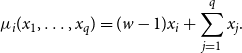 \begin{equation*} \mu _{i}(x_1,\ldots,x_q) = (w -1)x_i + \sum _{\substack {j=1}}^{q} x_j. \end{equation*}
Furthermore, we define
 \begin{equation*} \tilde {G}(x_1,\ldots, x_q) = \left (\mu _1(x_1,\ldots,x_{q}),\ldots,\mu _{q}(x_1,\ldots,x_{q}) \right ) \end{equation*}
and
 \begin{equation*} \tilde {F}(x_1,\ldots, x_q) = \tilde {G}(x_1^d,\ldots,x_{q}^d). \end{equation*}
Both $\tilde{F}$
and
$\tilde{F}$
and $\tilde{G}$
are homogeneous maps from
$\tilde{G}$
are homogeneous maps from $\mathbb{R}^{q}_{\gt 0}$
to itself. For
$\mathbb{R}^{q}_{\gt 0}$
to itself. For $x,y \in \mathbb{R}_{\gt 0}^{q}$
we define an equivalence relation
$x,y \in \mathbb{R}_{\gt 0}^{q}$
we define an equivalence relation $x\sim y$
if and only if
$x\sim y$
if and only if $x = \lambda y$
for some
$x = \lambda y$
for some $\lambda \gt 0$
. We define
$\lambda \gt 0$
. We define $\mathbb{P}^{q-1}_{\gt 0}= \mathbb{R}_{\gt 0}^{q}/ \sim$
and denote elements of
$\mathbb{P}^{q-1}_{\gt 0}= \mathbb{R}_{\gt 0}^{q}/ \sim$
and denote elements of $\mathbb{P}^{q-1}_{\gt 0}$
as
$\mathbb{P}^{q-1}_{\gt 0}$
as $[x_1\;:\;\ldots\;:\;x_q]$
. We note that since
$[x_1\;:\;\ldots\;:\;x_q]$
. We note that since $\tilde{F}$
and
$\tilde{F}$
and $\tilde{G}$
are homogeneous they are also well defined as maps from
$\tilde{G}$
are homogeneous they are also well defined as maps from $\mathbb{P}^{q-1}_{\gt 0}$
to itself and from now on we consider them as such.
$\mathbb{P}^{q-1}_{\gt 0}$
to itself and from now on we consider them as such.
Let $\pi\;:\;\mathbb{P}_{\gt 0}^{q-1} \to \mathbb{R}_{\gt 0}^{q-1}$
be the projection map defined by
$\pi\;:\;\mathbb{P}_{\gt 0}^{q-1} \to \mathbb{R}_{\gt 0}^{q-1}$
be the projection map defined by $\pi ([x_1\;:\ldots:\,\,x_q]) = (x_1/x_{q}, \ldots, x_{q-1}/x_{q})$
with inverse
$\pi ([x_1\;:\ldots:\,\,x_q]) = (x_1/x_{q}, \ldots, x_{q-1}/x_{q})$
with inverse $\iota\;:\;\mathbb{R}_{\gt 0}^{q-1} \to \mathbb{P}_{\gt 0}^{q-1}$
defined by
$\iota\;:\;\mathbb{R}_{\gt 0}^{q-1} \to \mathbb{P}_{\gt 0}^{q-1}$
defined by $\iota (x_1, \ldots, x_{q-1})=[x_1\;:\;\ldots\;:\;x_{q-1}\;:\;1]$
. Note that
$\iota (x_1, \ldots, x_{q-1})=[x_1\;:\;\ldots\;:\;x_{q-1}\;:\;1]$
. Note that $\pi$
and
$\pi$
and $\iota$
are continuous. We define the maps
$\iota$
are continuous. We define the maps $G,F$
from
$G,F$
from $\mathbb{R}_{\gt 0}^{q-1}$
to itself by
$\mathbb{R}_{\gt 0}^{q-1}$
to itself by $\pi \circ \tilde{G} \circ \iota$
and
$\pi \circ \tilde{G} \circ \iota$
and $\pi \circ \tilde{F} \circ \iota$
. Explicitly we have
$\pi \circ \tilde{F} \circ \iota$
. Explicitly we have
 \begin{equation*} G(x_1,x_2) = \left (\frac {w x_1 + x_2 + 1}{x_1+x_2+w},\frac {x_1 + w x_2 + 1}{x_1+x_2+w}\right )\ \text { and } \ F(x_1,x_2) = G(x_1^d,x_2^d) \end{equation*}
for $q=3$
. For
$q=3$
. For $q=4$
we have
$q=4$
we have
 \begin{equation*} G(x_1,x_2,x_3) = \left (\frac {w x_1 + x_2 + x_3 + 1}{x_1+x_2 + x_3 +w},\frac {x_1 + w x_2 + x_3 + 1}{x_1+x_2 + x_3 +w},\frac {x_1 + x_2 + w x_3 + 1}{x_1+x_2 + x_3 +w}\right ) \end{equation*}
and $F(x_1,x_2,x_3) = G(x_1^d,x_2^d,x_3^d)$
.
$F(x_1,x_2,x_3) = G(x_1^d,x_2^d,x_3^d)$
.
With this definition the recursion from Lemma 2.2 can now be stated as follows. Following the notation of the lemma, denote by $x_l$
the following log convex combination of the ratios
$x_l$
the following log convex combination of the ratios $R_{l,\tau _s}(\widehat{\mathbb{T}}^{n-1}_{d})$
,
$R_{l,\tau _s}(\widehat{\mathbb{T}}^{n-1}_{d})$
,
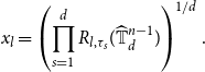 \begin{equation} x_l=\left (\prod _{s=1}^d R_{l,\tau _s}(\widehat{\mathbb{T}}^{n-1}_{d})\right )^{1/d}. \end{equation}
Then
 \begin{equation} \left (R_{1,\tau }(\widehat{\mathbb{T}}^{n}_{d}),\ldots,R_{q-1,\tau }(\widehat{\mathbb{T}}^{n}_{d})\right )=F(x_1,\ldots,x_{q-1}). \end{equation}
We say that a subset $\mathcal{T} \subseteq \mathbb{R}_{\gt 0}^n$
is log convex if
$\mathcal{T} \subseteq \mathbb{R}_{\gt 0}^n$
is log convex if $\log \!\left (\mathcal{T}\right )$
is a convex subset of
$\log \!\left (\mathcal{T}\right )$
is a convex subset of $\mathbb{R}^n$
, where
$\mathbb{R}^n$
, where $\log \!\left (\mathcal{T}\right )$
denotes the set consisting of elements of
$\log \!\left (\mathcal{T}\right )$
denotes the set consisting of elements of $\mathcal{T}$
with the logarithm applied to their individual entries. The next lemma gives sufficient conditions for uniqueness on the infinite regular tree.
$\mathcal{T}$
with the logarithm applied to their individual entries. The next lemma gives sufficient conditions for uniqueness on the infinite regular tree.
Lemma 2.3.
Suppose that $q\geq 2$
,
$q\geq 2$
, $d\geq 2$
and
$d\geq 2$
and $w\gt 0$
are such that there exists a sequence
$w\gt 0$
are such that there exists a sequence $\{\mathcal{T}_n\}_{n\geq 0}$
of log convex subsets of
$\{\mathcal{T}_n\}_{n\geq 0}$
of log convex subsets of $\mathbb{R}^{q-1}_{\gt 0}$
with the following properties.
$\mathbb{R}^{q-1}_{\gt 0}$
with the following properties.
-
(1) Both the vector with every entry equal to $1/w$
and the vectors obtained from the all-ones vector with a single entry changed to
$w$
are elements of
$\mathcal{T}_0$
.
$1/w$
and the vectors obtained from the all-ones vector with a single entry changed to
$w$
are elements of
$\mathcal{T}_0$
. -
(2) For every
$m$
we have
$F(\mathcal{T}_m) \subseteq \mathcal{T}_{m+1}$
. -
(3) For every
$\epsilon \gt 0$
there is an
$M$
such that for all
$m\geq M$
every element of
$\mathcal{T}_m$
has at most distance
$\epsilon$
to the all-ones vector.


Then the anti-ferromagnetic Potts model with parameter $w$
has has a unique Gibbs measure on
$w$
has has a unique Gibbs measure on $\mathbb{T}_{d}$
.
$\mathbb{T}_{d}$
.
Proof. By Lemma 2.1, it suffices to show that regardless of the boundary condition $\tau$
on
$\tau$
on $\Lambda _{n,d}$
,
$\Lambda _{n,d}$
, $R_{i,\tau }(\widehat{\mathbb{T}}_d^n)\to 1$
as
$R_{i,\tau }(\widehat{\mathbb{T}}_d^n)\to 1$
as $n\to \infty$
.
$n\to \infty$
.
First of all we claim that for all $n \geq 0$
and all boundary conditions
$n \geq 0$
and all boundary conditions $\tau\;:\;\Lambda _{n,d} \to [q]$
we have
$\tau\;:\;\Lambda _{n,d} \to [q]$
we have $(R_{1,\tau }(\widehat{\mathbb{T}}^{n}_{d}),\ldots,R_{q-1,\tau }(\widehat{\mathbb{T}}^{n}_{d})) \in \mathcal{T}_n$
. We prove this by induction on
$(R_{1,\tau }(\widehat{\mathbb{T}}^{n}_{d}),\ldots,R_{q-1,\tau }(\widehat{\mathbb{T}}^{n}_{d})) \in \mathcal{T}_n$
. We prove this by induction on $n$
. For the base case,
$n$
. For the base case, $n=0$
, we note that
$n=0$
, we note that $\widehat{\mathbb{T}}^0_{d}$
consists of one free root
$\widehat{\mathbb{T}}^0_{d}$
consists of one free root $\hat r_{d}$
, connected to a coloured vertex
$\hat r_{d}$
, connected to a coloured vertex $v$
. If
$v$
. If $v$
is coloured
$v$
is coloured $i \in [q-1]$
, then
$i \in [q-1]$
, then $(R_{1,\tau }(\widehat{\mathbb{T}}^{0}_{d}),\ldots,R_{q-1,\tau }(\widehat{\mathbb{T}}^{0}_{d}))$
consists of a
$(R_{1,\tau }(\widehat{\mathbb{T}}^{0}_{d}),\ldots,R_{q-1,\tau }(\widehat{\mathbb{T}}^{0}_{d}))$
consists of a $w$
on position
$w$
on position $i$
and ones everywhere else. If
$i$
and ones everywhere else. If $v$
is coloured
$v$
is coloured $q$
, then
$q$
, then $(R_{1,\tau }(\widehat{\mathbb{T}}^{0}_{d}),\ldots,R_{q-1,\tau }(\widehat{\mathbb{T}}^{0}_{d})) = (1/w, \ldots, 1/w)$
. So the base case follows from item (1).
$(R_{1,\tau }(\widehat{\mathbb{T}}^{0}_{d}),\ldots,R_{q-1,\tau }(\widehat{\mathbb{T}}^{0}_{d})) = (1/w, \ldots, 1/w)$
. So the base case follows from item (1).
Suppose next that for some $n \geq 0$
the claim holds. Let
$n \geq 0$
the claim holds. Let $\tau\;:\;\Lambda _{d,n+1} \to [q]$
be any boundary condition. It then follows from (7), (8) and the assumptions that
$\tau\;:\;\Lambda _{d,n+1} \to [q]$
be any boundary condition. It then follows from (7), (8) and the assumptions that $\mathcal{T}_n$
is log convex and
$\mathcal{T}_n$
is log convex and $F(\mathcal{T}_n)\subseteq (\mathcal{T}_{n+1})$
that
$F(\mathcal{T}_n)\subseteq (\mathcal{T}_{n+1})$
that
 \begin{equation*} \left (R_{1,\tau }(\widehat {\mathbb {T}}^{n}_{d}),\ldots,R_{q-1,\tau }(\widehat {\mathbb {T}}^{n}_{d})\right ) \in \mathcal {T}_{n+1}, \end{equation*}
completing the induction.
From the claim we just proved and item (3) it then follows that given $\varepsilon \gt 0$
there exists
$\varepsilon \gt 0$
there exists $N\gt 0$
such that for all
$N\gt 0$
such that for all $n\geq N$
, any boundary condition
$n\geq N$
, any boundary condition $\tau$
and color
$\tau$
and color $i$
,
$i$
, $|R_{i,\tau }(\widehat{\mathbb{T}}_d^n)- 1|\lt \varepsilon$
. This concludes the proof.
$|R_{i,\tau }(\widehat{\mathbb{T}}_d^n)- 1|\lt \varepsilon$
. This concludes the proof.
In the next section we will construct a sequence of regions $\{\mathcal{T}_n\}_{n \geq 0}$
satisfying the conditions of the lemma. In Subsection 3.1 we describe a certain symmetry that the map
$\{\mathcal{T}_n\}_{n \geq 0}$
satisfying the conditions of the lemma. In Subsection 3.1 we describe a certain symmetry that the map $F$
exhibits, corresponding to the symmetry of the colours in the Potts model. When a region
$F$
exhibits, corresponding to the symmetry of the colours in the Potts model. When a region $\mathcal{T}$
has a corresponding symmetry it is easier to understand the image
$\mathcal{T}$
has a corresponding symmetry it is easier to understand the image $F(\mathcal{T})$
. This is explained in Lemma 3.2. In Subsection 3.2 we define a two parameter family of sets
$F(\mathcal{T})$
. This is explained in Lemma 3.2. In Subsection 3.2 we define a two parameter family of sets $\mathcal{T}_{a,b}$
that display the required symmetry. In Lemma 3.4 we prove that if simple analytic conditions in
$\mathcal{T}_{a,b}$
that display the required symmetry. In Lemma 3.4 we prove that if simple analytic conditions in $a$
and
$a$
and $b$
are satisfied the sets
$b$
are satisfied the sets $\mathcal{T}_{a,b}$
are log-convex. In Lemma 3.6 we give inner and outer approximations of the sets
$\mathcal{T}_{a,b}$
are log-convex. In Lemma 3.6 we give inner and outer approximations of the sets $\mathcal{T}_{a,b}$
with simple polytopes. This is convenient since the map
$\mathcal{T}_{a,b}$
with simple polytopes. This is convenient since the map $G$
is a fractional linear transformation and therefore preserves convex sets. These are used in Lemma 3.7 in Subsection 3.3 where we show that if more involved analytical conditions are satisfied
$G$
is a fractional linear transformation and therefore preserves convex sets. These are used in Lemma 3.7 in Subsection 3.3 where we show that if more involved analytical conditions are satisfied $\mathcal{T}_{a,b}$
gets mapped strictly inside itself by
$\mathcal{T}_{a,b}$
gets mapped strictly inside itself by $F$
. We then combine all ingredients to prove the Main Theorem as Theorem 3.8. In the proof of Theorem 3.8 we show that we can construct a sequence
$F$
. We then combine all ingredients to prove the Main Theorem as Theorem 3.8. In the proof of Theorem 3.8 we show that we can construct a sequence $\mathcal{T}_n = \mathcal{T}_{a_n,b_n}$
that satisfies the conditions of Lemma 2.3 using the fact that we can keep satisfying the analytic conditions on
$\mathcal{T}_n = \mathcal{T}_{a_n,b_n}$
that satisfies the conditions of Lemma 2.3 using the fact that we can keep satisfying the analytic conditions on $a_n$
and
$a_n$
and $b_n$
. This uses a number of technical inequalities whose verification we have moved to Section 4 to preserve the flow of the text.
$b_n$
. This uses a number of technical inequalities whose verification we have moved to Section 4 to preserve the flow of the text.
We finish this section be providing proofs of Lemmas 2.1 and 2.2.
2.3 Proofs of Lemmas 2.1 and 2.2
Proof of Lemma
2.1
. The ratios for $\widehat{\mathbb{T}}^n_{d}$
and
$\widehat{\mathbb{T}}^n_{d}$
and $\mathbb{T}^n_{d}$
can easily be expressed in terms of each other. Fix any
$\mathbb{T}^n_{d}$
can easily be expressed in terms of each other. Fix any $\tau\;:\;\Lambda _{n,d}\to [q]$
. Then for any
$\tau\;:\;\Lambda _{n,d}\to [q]$
. Then for any $i=1,\ldots,q-1$
,
$i=1,\ldots,q-1$
,
 \begin{equation} R_{i,\tau }(\widehat{\mathbb{T}}_d^n)=\frac{(w-1) R_{i,\tau }(\mathbb{T}_d^n)+\sum _{j=1}^{q-1} R_{j,\tau }(\mathbb{T}_d^n)+1}{\sum _{j=1}^{q-1}R_{j,\tau }(\mathbb{T}_d^n)+w}\quad \text{ and } \quad R_{i,\tau }(\mathbb{T}_d^n)=(R_{i,\tau }(\widehat{\mathbb{T}}_d^{n-1}))^d. \end{equation}
We may thus assume that for each $\delta \gt 0$
there exist
$\delta \gt 0$
there exist $N'$
such that for all
$N'$
such that for all $n\geq N'$
,
$n\geq N'$
, $|R_{i,\tau }(\mathbb{T}_d^n)-1|\lt \delta$
for all
$|R_{i,\tau }(\mathbb{T}_d^n)-1|\lt \delta$
for all $\tau\;:\;\Lambda _{n,d}\to [q].$
For readability, we omit the reference to the subscript $d$
in what follows. For any
$d$
in what follows. For any $i=1,\ldots,q$
we have
$i=1,\ldots,q$
we have
 \begin{equation*} \mathbb {P}_{{\mathbb {T}}^{n}} [ {\boldsymbol \Phi }(r) = i \vert {\boldsymbol \Phi }\!\restriction _{\Lambda _n} = \tau ] = \frac {Z_{i,\tau }({\mathbb {T}}^{n})}{Z_{\tau }{(\mathbb {T}}^{n})} = \frac {Z_{i,\tau }({\mathbb {T}}^{n})}{\sum _{j=1}^q Z_{j,\tau }({\mathbb {T}}^{n})}. \end{equation*}
Hence for any $i \in [q]$
, upon dividing both the numerator and denominator by
$i \in [q]$
, upon dividing both the numerator and denominator by $Z_{q,\tau }({\mathbb{T}}^{n})$
, we obtain
$Z_{q,\tau }({\mathbb{T}}^{n})$
, we obtain
 \begin{equation*} \mathbb {P}_{{\mathbb {T}}^{n}} [ {\boldsymbol \Phi }(r) = i \vert {\boldsymbol \Phi }\!\restriction _{ \Lambda _n} = \tau ] = \frac {R_{i,\tau }(\mathbb {T}^{n})}{\sum _{i=1}^{q-1} R_{i,\tau }(\mathbb {T}^{n}) +1}. \end{equation*}
Now since the map
 \begin{equation*} (x_1, \ldots, x_{q-1}) \mapsto \max _{i \in [q-1]} \bigg ( \bigg \vert \frac {x_i}{\sum _{j=1}^{q-1} x_j +1} - \frac {1}{q}\bigg \vert, \bigg \vert \frac {1}{\sum _{j=1}^{q-1} x_j +1} - \frac {1}{q}\bigg \vert \bigg ) \end{equation*}
is continuous and maps $(1, \ldots, 1)$
to
$(1, \ldots, 1)$
to $0$
, it follows that for every
$0$
, it follows that for every $\epsilon \gt 0$
there is a
$\epsilon \gt 0$
there is a $\delta \gt 0$
such that
$\delta \gt 0$
such that $|R_{i,\tau }(\mathbb{T}_{n})-1| \lt \delta$
for all boundary conditions
$|R_{i,\tau }(\mathbb{T}_{n})-1| \lt \delta$
for all boundary conditions $\tau$
and
$\tau$
and $i=1.\ldots,q-1$
, implies that
$i=1.\ldots,q-1$
, implies that
 \begin{equation*} \max _{\tau:\Lambda _{n} \to [q]} \bigg \vert \mathbb {P}_{{\mathbb {T}}^{n}} [ {\boldsymbol \Phi }(r) = i \vert {\boldsymbol \Phi }\!\restriction _{\Lambda _n} = \tau ] - \frac {1}{q}\bigg \vert \lt \epsilon . \end{equation*}
We conclude that the conditions of Lemma 1.3 are satisfied and hence $\mathbb{T}_d$
has a unique Gibbs measure.
$\mathbb{T}_d$
has a unique Gibbs measure.
We next provide a proof for the tree recursion.
Proof of Lemma
2.2
. For readability we omit $d$
from the notation. We have
$d$
from the notation. We have
 \begin{equation} R_{i,\tau }(\widehat{\mathbb{T}}^{n}) = \frac{Z_{i,\tau }(\widehat{\mathbb{T}}^{n})}{Z_{q,\tau }(\widehat{\mathbb{T}}^{n})} = \frac{\sum _{l \in [q] \setminus \{i\}} Z_{l,\tau }({\mathbb{T}}^{n}) + w Z_{i,\tau }({\mathbb{T}}^{n})}{\sum _{l \in [q-1] } Z_{l,\tau }({\mathbb{T}}^{n}) + w Z_{q,\tau }({\mathbb{T}}^{n})}, \end{equation}
as a factor $w$
is picked up when the unique neighbour of the root vertex is assigned the same colour as the root vertex,
$w$
is picked up when the unique neighbour of the root vertex is assigned the same colour as the root vertex, $\hat{r}_d$
, of
$\hat{r}_d$
, of $\widehat{\mathbb{T}}^{n}$
. Note that for any color
$\widehat{\mathbb{T}}^{n}$
. Note that for any color $c \in [q]$
we have
$c \in [q]$
we have $Z_{c,\tau }({\mathbb{T}}^{n}) = \prod _{s=1}^{d} Z_{c,\tau _s}(\widehat{\mathbb{T}}^{n-1})$
. Plugging this in into (10) and dividing the numerator and denominator by
$Z_{c,\tau }({\mathbb{T}}^{n}) = \prod _{s=1}^{d} Z_{c,\tau _s}(\widehat{\mathbb{T}}^{n-1})$
. Plugging this in into (10) and dividing the numerator and denominator by $\prod _{s=1}^{d} Z_{q,\tau _s}(\widehat{\mathbb{T}}^{n-1})$
, we arrive at the desired expression.
$\prod _{s=1}^{d} Z_{q,\tau _s}(\widehat{\mathbb{T}}^{n-1})$
, we arrive at the desired expression.
3. Proof of the main theorem
In this section we use Lemma 2.3 to prove the Main Theorem.
3.1 Symmetry of the map
$\textbf{F}$

In order to find suitable sets $\mathcal{T}$
such that
$\mathcal{T}$
such that $F(\mathcal{T}) \subseteq \mathcal{T}$
we will exploit a symmetry that the map
$F(\mathcal{T}) \subseteq \mathcal{T}$
we will exploit a symmetry that the map $F$
exhibits, due to the inherent symmetry of permuting the colours
$F$
exhibits, due to the inherent symmetry of permuting the colours $[q]$
in the Potts model. To make this formal we will define a few self-maps on, and regions of, the spaces
$[q]$
in the Potts model. To make this formal we will define a few self-maps on, and regions of, the spaces $\mathbb{P}^{q-1}_{\gt 0}, \mathbb{R}^{q-1}_{\gt 0}$
and
$\mathbb{P}^{q-1}_{\gt 0}, \mathbb{R}^{q-1}_{\gt 0}$
and $\mathbb{R}^{q-1}$
. To avoid confusion, we will denote self-maps on and subsets of
$\mathbb{R}^{q-1}$
. To avoid confusion, we will denote self-maps on and subsets of $\mathbb{P}^{q-1}_{\gt 0}$
with a tilde, self-maps on and subsets of
$\mathbb{P}^{q-1}_{\gt 0}$
with a tilde, self-maps on and subsets of $\mathbb{R}^{q-1}_{\gt 0}$
without additional notation and self-maps on and subsets of
$\mathbb{R}^{q-1}_{\gt 0}$
without additional notation and self-maps on and subsets of $\mathbb{R}^{q-1}$
with a hat. When a self-map or subset is used as an index, we will drop the hat or tilde in the index.
$\mathbb{R}^{q-1}$
with a hat. When a self-map or subset is used as an index, we will drop the hat or tilde in the index.
The three spaces $\mathbb{P}^{q-1}_{\gt 0}, \mathbb{R}^{q-1}_{\gt 0}$
and
$\mathbb{P}^{q-1}_{\gt 0}, \mathbb{R}^{q-1}_{\gt 0}$
and $\mathbb{R}^{q-1}$
are homeomorphic, with homeomorphisms
$\mathbb{R}^{q-1}$
are homeomorphic, with homeomorphisms $\pi\;:\;\mathbb{P}_{\gt 0}^{q-1} \to \mathbb{R}_{\gt 0}^{q-1}$
with inverse
$\pi\;:\;\mathbb{P}_{\gt 0}^{q-1} \to \mathbb{R}_{\gt 0}^{q-1}$
with inverse $\iota$
and
$\iota$
and $\log\;:\;\mathbb{R}_{\gt 0}^{q-1} \to \mathbb{R}^{q-1}$
with inverse
$\log\;:\;\mathbb{R}_{\gt 0}^{q-1} \to \mathbb{R}^{q-1}$
with inverse $\exp$
. We define the self-maps
$\exp$
. We define the self-maps $\hat{G},\hat{F}$
on
$\hat{G},\hat{F}$
on $\mathbb{R}^{q-1}$
by
$\mathbb{R}^{q-1}$
by $\hat{G} = \log \circ{G} \circ \exp$
and
$\hat{G} = \log \circ{G} \circ \exp$
and $\hat{F} = \log \circ{F} \circ \exp$
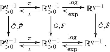
. To summarise, we have the following diagram of continuous maps
$\hat{F} = \log \circ{F} \circ \exp$
. To summarise, we have the following diagram of continuous maps
Let $S_q$
denote the symmetric group on
$S_q$
denote the symmetric group on $q$
elements. This group acts on
$q$
elements. This group acts on $\mathbb{P}^{q-1}_{\gt 0}$
be permuting the entries, which corresponds to permuting the colours in the Potts model. For
$\mathbb{P}^{q-1}_{\gt 0}$
be permuting the entries, which corresponds to permuting the colours in the Potts model. For $\sigma \in S_q$
we denote the map from
$\sigma \in S_q$
we denote the map from $\mathbb{P}^{q-1}_{\gt 0}$
to itself corresponding to this action by
$\mathbb{P}^{q-1}_{\gt 0}$
to itself corresponding to this action by $\tilde{M}_\sigma$
. We use this action to also define an action on
$\tilde{M}_\sigma$
. We use this action to also define an action on $\mathbb{R}_{\gt 0}^{q-1}$
by letting
$\mathbb{R}_{\gt 0}^{q-1}$
by letting $M_\sigma (x) = (\pi \circ \tilde{M}_\sigma \circ \iota )(x)$
. It is easy to see that the action of
$M_\sigma (x) = (\pi \circ \tilde{M}_\sigma \circ \iota )(x)$
. It is easy to see that the action of $S_q$
on
$S_q$
on $\mathbb{P}_{\gt 0}^{q-1}$
commutes with
$\mathbb{P}_{\gt 0}^{q-1}$
commutes with $\tilde{G}$
and
$\tilde{G}$
and $\tilde{F}$
. It follows that the action of
$\tilde{F}$
. It follows that the action of $S_q$
on
$S_q$
on $\mathbb{R}_{\gt 0}^{q-1}$
also commutes with
$\mathbb{R}_{\gt 0}^{q-1}$
also commutes with $F$
and
$F$
and $G$
. Similarly, we define the map
$G$
. Similarly, we define the map $\hat{M}_\sigma$
on
$\hat{M}_\sigma$
on $x \in \mathbb{R}^{q-1}$
by
$x \in \mathbb{R}^{q-1}$
by $\hat{M}_\sigma (x) = \left (\log \circ M_\sigma \circ \exp \right )\!(x)$
and we note that this action commutes with
$\hat{M}_\sigma (x) = \left (\log \circ M_\sigma \circ \exp \right )\!(x)$
and we note that this action commutes with $\hat{G}$
and
$\hat{G}$
and $\hat{F}$
.
$\hat{F}$
.
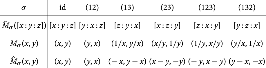
Example 3.1. As an example we present the table of the action of $S_q$
for
$S_q$
for $q=3$
on a point in all the three coordinates.
$q=3$
on a point in all the three coordinates.
The three spaces $\mathbb{P}^{q-1}_{\gt 0}, \mathbb{R}^{q-1}_{\gt 0}$
and
$\mathbb{P}^{q-1}_{\gt 0}, \mathbb{R}^{q-1}_{\gt 0}$
and $\mathbb{R}^{q-1}$
are homeomorphic, with homeomorphisms
$\mathbb{R}^{q-1}$
are homeomorphic, with homeomorphisms $\pi\;:\;\mathbb{P}_{\gt 0}^{q-1} \to \mathbb{R}_{\gt 0}^{q-1}$
with inverse
$\pi\;:\;\mathbb{P}_{\gt 0}^{q-1} \to \mathbb{R}_{\gt 0}^{q-1}$
with inverse $\iota$
and
$\iota$
and $\log\;:\;\mathbb{R}_{\gt 0}^{q-1} \to \mathbb{R}^{q-1}$
with inverse
$\log\;:\;\mathbb{R}_{\gt 0}^{q-1} \to \mathbb{R}^{q-1}$
with inverse $\exp$
. We define the self-maps
$\exp$
. We define the self-maps $\hat{G},\hat{F}$
on
$\hat{G},\hat{F}$
on $\mathbb{R}^{q-1}$
by
$\mathbb{R}^{q-1}$
by $\hat{G} = \log \circ{G} \circ \exp$
and
$\hat{G} = \log \circ{G} \circ \exp$
and $\hat{F} = \log \circ{F} \circ \exp$
. To summarise, we have the following diagram of continuous maps
$\hat{F} = \log \circ{F} \circ \exp$
. To summarise, we have the following diagram of continuous maps
Note that in general $\hat{M}_\sigma$
is a linear map for all
$\hat{M}_\sigma$
is a linear map for all $\sigma \in S_q$
. In fact, the map
$\sigma \in S_q$
. In fact, the map $\sigma \mapsto \hat{M}_\sigma$
is an irreducible representation of
$\sigma \mapsto \hat{M}_\sigma$
is an irreducible representation of $S_q$
called the standard representation, but we will not use this.
$S_q$
called the standard representation, but we will not use this.
For any permutation $\tau \in S_q$
we define the following subset of
$\tau \in S_q$
we define the following subset of $\mathbb{P}_{\gt 0}^{q-1}$
 \begin{equation*} \tilde {\mathcal {R}}_{\tau } = \left \{[x_1\;:\;\ldots\;:\;x_q] \in \mathbb {P}_{\gt 0}^{q-1}\;:\;x_{\tau (1)} \leq x_{\tau (2)} \leq \cdots \leq x_{\tau (k)} \right \}. \end{equation*}
Furthermore, we let $\mathcal{R}_\tau = \pi (\tilde{\mathcal{R}}_{\tau })$
and
$\mathcal{R}_\tau = \pi (\tilde{\mathcal{R}}_{\tau })$
and $\hat{\mathcal{R}}_\tau = \log\!(\mathcal{R}_\tau )$
. Note that if
$\hat{\mathcal{R}}_\tau = \log\!(\mathcal{R}_\tau )$
. Note that if $x\in \mathbb{P}_{\gt 0}^{q-1}$
has the property that
$x\in \mathbb{P}_{\gt 0}^{q-1}$
has the property that $x_i \geq x_j$
then
$x_i \geq x_j$
then $\mu _{i}(x) \leq \mu _{j}(x)$
, recalling that
$\mu _{i}(x) \leq \mu _{j}(x)$
, recalling that
 \begin{equation*} \mu _{i}(x_1,\ldots,x_q) = (w -1)x_i + \sum _{\substack {j=1}}^{q} x_j. \end{equation*}
It follows that the map $\tilde{G}$
maps
$\tilde{G}$
maps $\tilde{\mathcal{R}}_\tau$
into
$\tilde{\mathcal{R}}_\tau$
into $\tilde{\mathcal{R}}_{\tau \circ m}$
, where
$\tilde{\mathcal{R}}_{\tau \circ m}$
, where $m \in S_q$
denotes the permutation with
$m \in S_q$
denotes the permutation with $m(l) = k+1-l$
for
$m(l) = k+1-l$
for $l \in [q]$
. The same is true for
$l \in [q]$
. The same is true for $\tilde{F}$
because
$\tilde{F}$
because $x \mapsto x^d$
maps any
$x \mapsto x^d$
maps any $\tilde{\mathcal{R}}_\tau$
to itself. It follows that
$\tilde{\mathcal{R}}_\tau$
to itself. It follows that $G$
and
$G$
and $F$
map
$F$
map $\mathcal{R}_\tau$
into
$\mathcal{R}_\tau$
into $\mathcal{R}_{\tau \circ m}$
and that
$\mathcal{R}_{\tau \circ m}$
and that $\hat{G}$
and
$\hat{G}$
and $\hat{F}$
map
$\hat{F}$
map $\hat{\mathcal{R}}_\tau$
into
$\hat{\mathcal{R}}_\tau$
into $\hat{\mathcal{R}}_{\tau \circ m}$
. In Figure 1 the regions
$\hat{\mathcal{R}}_{\tau \circ m}$
. In Figure 1 the regions $\mathcal{R}_\tau$
and
$\mathcal{R}_\tau$
and $\hat{\mathcal{R}}_\tau$
are depicted when
$\hat{\mathcal{R}}_\tau$
are depicted when $q =3$
.
$q =3$
.
The main purpose of the considerations of this section up until this point is to state and prove the following simple lemma.
Lemma 3.2.
Suppose $\mathcal{T} \subseteq \mathbb{R}_{\gt 0}^{q-1}$
is a set such that
$\mathcal{T} \subseteq \mathbb{R}_{\gt 0}^{q-1}$
is a set such that $M_\sigma (\mathcal{T}) = \mathcal{T}$
for all
$M_\sigma (\mathcal{T}) = \mathcal{T}$
for all $\sigma \in S_q$
. Suppose also that there is a permutation
$\sigma \in S_q$
. Suppose also that there is a permutation $\tau \in S_q$
such that
$\tau \in S_q$
such that
 \begin{equation*} F\!\left (\mathcal {T} \cap \mathcal {R}_{\tau } \right ) \subseteq \text {int}(\mathcal {T}). \end{equation*}
Then $F(\mathcal{T}) \subseteq \text{int}(\mathcal{T})$
.
$F(\mathcal{T}) \subseteq \text{int}(\mathcal{T})$
.
Proof. Let $x \in \mathcal{T}$
. There is a
$x \in \mathcal{T}$
. There is a $\sigma \in S_q$
such that
$\sigma \in S_q$
such that $M_\sigma (x) \in \mathcal{R}_{\tau }$
and thus
$M_\sigma (x) \in \mathcal{R}_{\tau }$
and thus $M_\sigma (x) \in \mathcal{T} \cap \mathcal{R}_{\tau }$
. It follows from the assumption that
$M_\sigma (x) \in \mathcal{T} \cap \mathcal{R}_{\tau }$
. It follows from the assumption that $(F\circ M_\sigma )(x) \in \text{int}(\mathcal{T})$
. Because
$(F\circ M_\sigma )(x) \in \text{int}(\mathcal{T})$
. Because $M_\sigma$
commutes with
$M_\sigma$
commutes with $F$
we find that
$F$
we find that $(M_\sigma \circ F)(x) \in \text{int}(\mathcal{T})$
. We conclude that
$(M_\sigma \circ F)(x) \in \text{int}(\mathcal{T})$
. We conclude that $F(x) \in M_\sigma ^{-1}(\text{int}(\mathcal{T}))=M_{\sigma ^{-1}}(\text{int}(\mathcal{T}))\subseteq \mathcal{T}$
. Because
$F(x) \in M_\sigma ^{-1}(\text{int}(\mathcal{T}))=M_{\sigma ^{-1}}(\text{int}(\mathcal{T}))\subseteq \mathcal{T}$
. Because $M_\sigma$
is continuous it follows that
$M_\sigma$
is continuous it follows that $M_\sigma ^{-1}(\text{int}(\mathcal{T}))$
is an open subset of
$M_\sigma ^{-1}(\text{int}(\mathcal{T}))$
is an open subset of $\mathcal{T}$
and hence
$\mathcal{T}$
and hence $F(x) \in \text{int}(\mathcal{T})$
.
$F(x) \in \text{int}(\mathcal{T})$
.
In the next section we will define a family of regions $\mathcal{T}_{a,b}$
for
$\mathcal{T}_{a,b}$
for $a,b\gt 1$
with the property
$a,b\gt 1$
with the property $M_\sigma (\mathcal{T}_{a,b})=\mathcal{T}_{a,b}$
for all
$M_\sigma (\mathcal{T}_{a,b})=\mathcal{T}_{a,b}$
for all $\sigma \in S_q$
. Our goal will be to show that for certain choices of parameters
$\sigma \in S_q$
. Our goal will be to show that for certain choices of parameters $(a,b)$
we have
$(a,b)$
we have $F(\mathcal{T}_{a,b}) \subseteq \text{int}(T_{a,b})$
. Because of Lemma 3.2 it will be enough to restrict ourselves to one well chosen region
$F(\mathcal{T}_{a,b}) \subseteq \text{int}(T_{a,b})$
. Because of Lemma 3.2 it will be enough to restrict ourselves to one well chosen region $\mathcal{R}_{\tau }$
.
$\mathcal{R}_{\tau }$
.
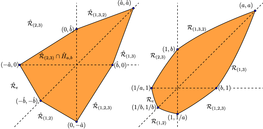
Figure 1. Images for $q=3$
of
$q=3$
of $\hat{\mathcal{T}}_{a,b}$
on the left and
$\hat{\mathcal{T}}_{a,b}$
on the left and $\mathcal{T}_{a,b}$
on the right. The boundaries of the regions
$\mathcal{T}_{a,b}$
on the right. The boundaries of the regions $\hat{\mathcal{R}}_\tau$
and
$\hat{\mathcal{R}}_\tau$
and $\mathcal{R}_\tau$
are drawn with dashed lines.
$\mathcal{R}_\tau$
are drawn with dashed lines.
3.2 Definition and properties of the sets
$\boldsymbol{\mathcal{T}\!}_{\textbf{a,b}}$

For $q=3$
and
$q=3$
and $q=4$
we will define a family of log convex sets
$q=4$
we will define a family of log convex sets $\mathcal{T}_{a,b}\subseteq \mathbb{R}_{\gt 0}^{q-1}$
with the property that
$\mathcal{T}_{a,b}\subseteq \mathbb{R}_{\gt 0}^{q-1}$
with the property that $M_\sigma (\mathcal{T}_{a,b}) = \mathcal{T}_{a,b}$
for all
$M_\sigma (\mathcal{T}_{a,b}) = \mathcal{T}_{a,b}$
for all $\sigma \in S_q$
. We will do this by defining the convex sets
$\sigma \in S_q$
. We will do this by defining the convex sets $\hat{\mathcal{T}}_{a,b} \subseteq \mathbb{R}^{q-1}$
and then letting
$\hat{\mathcal{T}}_{a,b} \subseteq \mathbb{R}^{q-1}$
and then letting $\mathcal{T}_{a,b} = \exp\!(\hat{\mathcal{T}}_{a,b})$
.
$\mathcal{T}_{a,b} = \exp\!(\hat{\mathcal{T}}_{a,b})$
.
Let $a,b\gt 1$
. To avoid having to write too many logarithms we let
$a,b\gt 1$
. To avoid having to write too many logarithms we let $\hat{a} = \log\!(a)$
and
$\hat{a} = \log\!(a)$
and $\hat{b} = \log\!(b)$
. For
$\hat{b} = \log\!(b)$
. For $q=3$
we define the following half-space of
$q=3$
we define the following half-space of $\mathbb{R}^2$
 \begin{equation*} \hat {H}_{a,b} = \{(x,y) \in \mathbb {R}^2\;:-\hat {b}\cdot x + \hat {a}\cdot y \leq \hat {a}\hat {b}\}. \end{equation*}
Subsequently, we define
 \begin{equation*} \hat {\mathcal {T}}_{a,b} = \bigcup _{\sigma \in S_3}\hat {M}_\sigma \!\left (\hat {\mathcal {R}}_{(23)} \cap \hat {H}_{a,b}\right ). \end{equation*}
Similarly, for $q=4$
, we define the half-space
$q=4$
, we define the half-space
 \begin{equation*} \hat {H}_{a,b} = \{(x,y,z) \in \mathbb {R}^3\;:-\hat {b}\cdot x + \hat {a}\cdot z \leq \hat {a}\hat {b}\} \end{equation*}
and the region
 \begin{equation*} \hat {\mathcal {T}}_{a,b} = \bigcup _{\sigma \in S_4}\hat {M}_\sigma \!\left (\hat {\mathcal {R}}_{(243)} \cap \hat {H}_{a,b}\right ). \end{equation*}
For both $q=3$
and
$q=3$
and $q=4$
we let
$q=4$
we let $\mathcal{T}_{a,b} = \exp\!(\hat{\mathcal{T}}_{a,b})$
. Figure 1 contains an image of
$\mathcal{T}_{a,b} = \exp\!(\hat{\mathcal{T}}_{a,b})$
. Figure 1 contains an image of $\hat{\mathcal{T}}_{a,b}$
and
$\hat{\mathcal{T}}_{a,b}$
and $\mathcal{T}_{a,b}$
for
$\mathcal{T}_{a,b}$
for $q=3$
. Figure 2 contains an image of
$q=3$
. Figure 2 contains an image of $\hat{\mathcal{T}}_{a,b}$
for
$\hat{\mathcal{T}}_{a,b}$
for $q=4$
; we highlighted the region
$q=4$
; we highlighted the region $\hat{\mathcal{R}}_{(243)} \cap \hat{H}_{a,b}$
in orange. We have chosen to give the sets
$\hat{\mathcal{R}}_{(243)} \cap \hat{H}_{a,b}$
in orange. We have chosen to give the sets $\hat{\mathcal{T}}_{a,b}$
the same name for
$\hat{\mathcal{T}}_{a,b}$
the same name for $q=3$
and
$q=3$
and $q=4$
. This is because many of the properties of
$q=4$
. This is because many of the properties of $\hat{\mathcal{T}}_{a,b}$
that we will prove hold for both cases and are proved in a similar way. Unless otherwise stated one should assume that any statement involving
$\hat{\mathcal{T}}_{a,b}$
that we will prove hold for both cases and are proved in a similar way. Unless otherwise stated one should assume that any statement involving $\hat{\mathcal{T}}_{a,b}$
refers to the corresponding statement for both
$\hat{\mathcal{T}}_{a,b}$
refers to the corresponding statement for both $q=3$
and
$q=3$
and $q=4$
.
$q=4$
.
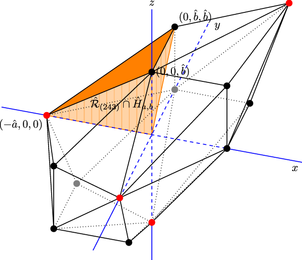
Figure 2. Image for $q=4$
of
$q=4$
of $\hat{\mathcal{T}}_{a,b}$
. The red dots depend on
$\hat{\mathcal{T}}_{a,b}$
. The red dots depend on $\hat{a}$
while the black dots depend on
$\hat{a}$
while the black dots depend on $\hat{b}$
. In orange the region
$\hat{b}$
. In orange the region $\hat{\mathcal{R}}_{(243)} \cap \hat{H}_{a,b}$
is depicted.
$\hat{\mathcal{R}}_{(243)} \cap \hat{H}_{a,b}$
is depicted.
We first state a basic lemma relating the half-space representation and the vertex representation of a polytope. This lemma will be used a number of times in the remainder of the section to derive useful properties of the sets $\mathcal{T}_{a,b}$
.
$\mathcal{T}_{a,b}$
.
Lemma 3.3.
Let $H_1, \ldots, H_n$
be closed half-spaces in
$H_1, \ldots, H_n$
be closed half-spaces in $\mathbb{R}^{n-1}$
. Furthermore, let
$\mathbb{R}^{n-1}$
. Furthermore, let $p_1, \ldots, p_n \in \mathbb{R}^{n-1}$
with the property that for all
$p_1, \ldots, p_n \in \mathbb{R}^{n-1}$
with the property that for all $i \in [n]$
we have
$i \in [n]$
we have $p_i \in \text{int}(H_i)$
and
$p_i \in \text{int}(H_i)$
and $p_i \in \partial H_j$
for
$p_i \in \partial H_j$
for $j \neq i$
. Then
$j \neq i$
. Then
 \begin{equation*} \bigcap _{i=1}^n H_i = \text{Conv}\!\left (\{p_1,\ldots, p_n\}\right ), \end{equation*}
where $\text{Conv}(S)$
denotes the convex hull of the set
$\text{Conv}(S)$
denotes the convex hull of the set $S$
.
$S$
.
Proof. We give a sketch of the proof. The conditions on the $p_i$
imply that the set
$p_i$
imply that the set $\{p_1, \ldots, p_n\}$
is affinely independent, i.e. the set
$\{p_1, \ldots, p_n\}$
is affinely independent, i.e. the set $\{p_1-p_n, \ldots, p_{n-1}-p_n\}$
is linearly independent. Therefore there exists an invertible affine transformation
$\{p_1-p_n, \ldots, p_{n-1}-p_n\}$
is linearly independent. Therefore there exists an invertible affine transformation $T$
with
$T$
with $T(v) = M(v-p_n)$
for some invertible linear transformation
$T(v) = M(v-p_n)$
for some invertible linear transformation $M$
, such that
$M$
, such that $T(p_i) = e_i$
for
$T(p_i) = e_i$
for $i \in [n-1]$
, where
$i \in [n-1]$
, where $e_i$
denotes a standard basis vector. From the conditions on the
$e_i$
denotes a standard basis vector. From the conditions on the $p_i$
it follows that
$p_i$
it follows that $T(H_i) = \{x \in \mathbb{R}^{n-1}\;:\;x_i \geq 0 \}$
for
$T(H_i) = \{x \in \mathbb{R}^{n-1}\;:\;x_i \geq 0 \}$
for $i \in [n-1]$
and
$i \in [n-1]$
and $T(H_n) = \{x \in \mathbb{R}^{n-1}\;:\;\sum _{i=1}^{n-1} x_i \leq 1\}$
. As affine transformations preserve convexity, we see
$T(H_n) = \{x \in \mathbb{R}^{n-1}\;:\;\sum _{i=1}^{n-1} x_i \leq 1\}$
. As affine transformations preserve convexity, we see
 \begin{align*} T\left (\bigcap _{i=1}^n H_i\right ) &= \bigcap _{i=1}^n T(H_i) = \bigcap _{i=1}^{n-1} \{x \in \mathbb{R}^{n-1}\;:\;x_i \geq 0 \} \cap \{x \in \mathbb{R}^{n-1}\;:\;\sum _{i=1}^{n-1} x_i \leq 1\}\\[5pt] &= \text{Conv}\!\left (\{e_1,\ldots, e_{n-1},0\}\right ) = \text{Conv}\!\left (\{T(p_1), \ldots, T(p_n)\}\right ) = T\!\left (\text{Conv}\!\left (\{p_1,\ldots, p_n\} \right )\right ). \end{align*}
The lemma now follows from the fact that $T$
is invertible.
$T$
is invertible.
Lemma 3.4.
For $a,b \in \mathbb{R}_{\gt 1}$
with
$a,b \in \mathbb{R}_{\gt 1}$
with $b\leq a \leq b^2$
we have that
$b\leq a \leq b^2$
we have that $\hat{\mathcal{T}}_{a,b}$
is convex, or equivalently, that
$\hat{\mathcal{T}}_{a,b}$
is convex, or equivalently, that $\mathcal{T}_{a,b}$
is log convex.
$\mathcal{T}_{a,b}$
is log convex.
Proof. Recall that we let $\hat{a} = \log\!(a)$
and
$\hat{a} = \log\!(a)$
and $\hat{b} = \log\!(b)$
and observe that these are two positive real numbers. Also recall that the action of
$\hat{b} = \log\!(b)$
and observe that these are two positive real numbers. Also recall that the action of $S_q$
on
$S_q$
on $\mathbb{R}^{q-1}$
is given by linear maps. It follows that the half-space
$\mathbb{R}^{q-1}$
is given by linear maps. It follows that the half-space $\hat{H}_{a,b}$
gets mapped to a half-space by
$\hat{H}_{a,b}$
gets mapped to a half-space by $\hat{M}_\sigma$
for any
$\hat{M}_\sigma$
for any $\sigma \in S_q$
. We will show that for the choices of parameters stated in the lemma we have
$\sigma \in S_q$
. We will show that for the choices of parameters stated in the lemma we have
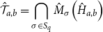 \begin{equation} \hat{\mathcal{T}}_{a,b} = \bigcap _{\sigma \in S_q}\hat{M}_\sigma \!\left (\hat{H}_{a,b}\right ) \end{equation}
for both $q=3$
and
$q=3$
and $q=4$
. This equality implies that
$q=4$
. This equality implies that $\hat{\mathcal{T}}_{a,b}$
is convex because an intersection of half-spaces is convex. In fact, it implies that
$\hat{\mathcal{T}}_{a,b}$
is convex because an intersection of half-spaces is convex. In fact, it implies that $\hat{\mathcal{T}}_{a,b}$
is a convex polytope.
$\hat{\mathcal{T}}_{a,b}$
is a convex polytope.
We will first prove that the right-hand side of (10) is contained in the left-hand side. To that effect take an element $x \in \bigcap _{\sigma \in S_q}\hat{M}_\sigma \!\left (\hat{H}_{a,b}\right )$
. Because the collection
$x \in \bigcap _{\sigma \in S_q}\hat{M}_\sigma \!\left (\hat{H}_{a,b}\right )$
. Because the collection $\{\hat{\mathcal{R}}_{\sigma }\}_{\sigma \in S_q}$
covers
$\{\hat{\mathcal{R}}_{\sigma }\}_{\sigma \in S_q}$
covers $\mathbb{R}^{q-1}$
, there is a
$\mathbb{R}^{q-1}$
, there is a $\tau \in S_q$
such that
$\tau \in S_q$
such that $x \in \hat{\mathcal{R}}_{\tau }$
. For
$x \in \hat{\mathcal{R}}_{\tau }$
. For $q = 3$
let
$q = 3$
let $\sigma \in S_3$
such that
$\sigma \in S_3$
such that $\sigma \cdot (23) = \tau$
. We see that
$\sigma \cdot (23) = \tau$
. We see that $x \in \hat{\mathcal{R}}_{\tau }\cap \hat{M}_\sigma (\hat{H}_{a,b})$
and thus
$x \in \hat{\mathcal{R}}_{\tau }\cap \hat{M}_\sigma (\hat{H}_{a,b})$
and thus $x \in \hat{M}_\sigma \left (\hat{\mathcal{R}}_{(23)}\cap \hat{H}_{a,b}\right )$
, from which it follows
$x \in \hat{M}_\sigma \left (\hat{\mathcal{R}}_{(23)}\cap \hat{H}_{a,b}\right )$
, from which it follows $x \in \hat{\mathcal{T}}_{a,b}$
. Similarly, for
$x \in \hat{\mathcal{T}}_{a,b}$
. Similarly, for $q=4$
we let
$q=4$
we let $\sigma \in S_4$
such that
$\sigma \in S_4$
such that $\sigma \cdot (243) = \tau$
. It follows in exactly the same way that
$\sigma \cdot (243) = \tau$
. It follows in exactly the same way that $x \in \hat{\mathcal{T}}_{a,b}$
.
$x \in \hat{\mathcal{T}}_{a,b}$
.
The proof that the left-hand side of (10) is contained in the right-hand side is slightly more involved. Assume that $q=3$
. We first show that
$q=3$
. We first show that
 \begin{equation} \hat{\mathcal{R}}_{(23)} \cap \hat{H}_{a,b} = \text{Conv}\!\left (\{(0,0),(\!-\hat{a},0),(0,\hat{b})\}\right ), \end{equation}
While this is easily seen to be true from Figure 1, we provide a formal proof. Note that $\hat{\mathcal{R}}_{(23)}$
is the intersection of
$\hat{\mathcal{R}}_{(23)}$
is the intersection of $\hat{H}_{x\leq 0} = \{(x,y) \in \mathbb{R}^2\;:\;x \leq 0\}$
and
$\hat{H}_{x\leq 0} = \{(x,y) \in \mathbb{R}^2\;:\;x \leq 0\}$
and $\hat{H}_{y \geq 0} = \{(x,y) \in \mathbb{R}^2\;:\;y \geq 0\}$
. One can check that
$\hat{H}_{y \geq 0} = \{(x,y) \in \mathbb{R}^2\;:\;y \geq 0\}$
. One can check that $(0,0) \in \partial \hat{H}_{x\leq 0} \cap \partial \hat{H}_{y\geq 0}\cap \text{int}(\hat{H}_{a,b})$
,
$(0,0) \in \partial \hat{H}_{x\leq 0} \cap \partial \hat{H}_{y\geq 0}\cap \text{int}(\hat{H}_{a,b})$
, $(\!-\hat{a},0) \in \partial \hat{H}_{a,b} \cap \partial \hat{H}_{y\geq 0}\cap \text{int}(\hat{H}_{x\leq 0} )$
and
$(\!-\hat{a},0) \in \partial \hat{H}_{a,b} \cap \partial \hat{H}_{y\geq 0}\cap \text{int}(\hat{H}_{x\leq 0} )$
and $(0,\hat{b}) \in \partial \hat{H}_{a,b} \cap \partial \hat{H}_{x\leq 0}\cap \text{int}(\hat{H}_{y\geq 0} )$
. Equation (12) then follows from Lemma 3.3.
$(0,\hat{b}) \in \partial \hat{H}_{a,b} \cap \partial \hat{H}_{x\leq 0}\cap \text{int}(\hat{H}_{y\geq 0} )$
. Equation (12) then follows from Lemma 3.3.
We obtain
 \begin{equation*} \hat {\mathcal {T}}_{a,b} = \bigcup _{\sigma \in S_3}\hat {M}_\sigma \!\left (\text {Conv}\!\left (\{(0,0),(\!-\hat {a},0),(0,\hat {b})\}\right )\right ) = \bigcup _{\sigma \in S_3}\text {Conv}\!\left (\{(0,0),\hat {M}_\sigma (\!-\hat {a},0),\hat {M}_\sigma (0,\hat {b})\}\right ). \end{equation*}
We want to show that this is a subset of $\bigcap _{\sigma \in S_3}\hat{M}_\sigma \left (\hat{H}_{a,b}\right )$
. Because all these half-spaces are convex, it is enough to show that the set
$\bigcap _{\sigma \in S_3}\hat{M}_\sigma \left (\hat{H}_{a,b}\right )$
. Because all these half-spaces are convex, it is enough to show that the set $P = \{(0,0)\} \cup \bigcup _{\sigma \in S_3} \{\hat{M}_\sigma (\!-\hat{a},0),\hat{M}_\sigma (0,\hat{b})\}$
is a subset of
$P = \{(0,0)\} \cup \bigcup _{\sigma \in S_3} \{\hat{M}_\sigma (\!-\hat{a},0),\hat{M}_\sigma (0,\hat{b})\}$
is a subset of $\hat{M}_\tau (H_{a,b})$
for all
$\hat{M}_\tau (H_{a,b})$
for all $\tau \in S_3$
. Because the set
$\tau \in S_3$
. Because the set $P$
is invariant under the action of
$P$
is invariant under the action of $S_3$
it is sufficient to show that
$S_3$
it is sufficient to show that $P \subseteq \hat{H}_{a,b}$
. We can calculate
$P \subseteq \hat{H}_{a,b}$
. We can calculate $P$
explicitly to obtain
$P$
explicitly to obtain
 \begin{equation*} P = \{(0,0),(0, -\hat {a}), (\!-\hat {a}, 0), (\hat {a}, \hat {a}),(0, \hat {b}), (\hat {b}, 0),(\!-\hat {b}, -\hat {b})\}. \end{equation*}
To check that these points lie in $\hat{H}_{a,b}$
we have to check that for each
$\hat{H}_{a,b}$
we have to check that for each $(x,y) \in P$
we have
$(x,y) \in P$
we have $-\hat{b}\cdot x + \hat{a}\cdot y \leq \hat{a}\hat{b}$
. The inequality is trivially true for all but the points
$-\hat{b}\cdot x + \hat{a}\cdot y \leq \hat{a}\hat{b}$
. The inequality is trivially true for all but the points $(\hat{a}, \hat{a})$
and
$(\hat{a}, \hat{a})$
and $(\!-\hat{b}, -\hat{b})$
. One can confirm that the inequalities obtained by filling in these two points are simultaneously satisfied if and only if
$(\!-\hat{b}, -\hat{b})$
. One can confirm that the inequalities obtained by filling in these two points are simultaneously satisfied if and only if $\hat{b}/2 \leq \hat{a} \leq 2\hat{b}$
. Because
$\hat{b}/2 \leq \hat{a} \leq 2\hat{b}$
. Because $\hat{a} = \log\!(a)$
and
$\hat{a} = \log\!(a)$
and $\hat{b}= \log\!(b)$
this is equivalent to
$\hat{b}= \log\!(b)$
this is equivalent to $\sqrt{b} \leq a \leq b^2$
. This shows that for these choices of
$\sqrt{b} \leq a \leq b^2$
. This shows that for these choices of $a$
and
$a$
and $b$
the left-hand side of (11) is contained in the right-hand side, which concludes the proof for
$b$
the left-hand side of (11) is contained in the right-hand side, which concludes the proof for $q=3$
.
$q=3$
.
The proof for $q=4$
follows the same path. One can show in very similar way to the
$q=4$
follows the same path. One can show in very similar way to the $q=3$
case that
$q=3$
case that
 \begin{equation*} \hat {\mathcal {R}}_{(243)} \cap \hat {H}_{a,b} = \text {Conv}\!\left (\{(0,0,0),(\!-\hat {a},0,0),(0,0,\hat {b}),(0,\hat {b},\hat {b})\}\right ) \end{equation*}
and thus that
 \begin{equation*} \hat {\mathcal {T}}_{a,b} = \bigcup _{\sigma \in S_4}\text {Conv}\!\left (\{(0,0,0),\hat {M}_\sigma (\!-\hat {a},0,0),\hat {M}_\sigma (0,0,\hat {b}),\hat {M}_\sigma (0,\hat {b},\hat {b})\}\right ). \end{equation*}
It is again sufficient to show that $P = \{(0,0,0)\} \cup \bigcup _{\sigma \in S_4} \{\hat{M}_\sigma (\!-\hat{a},0,0),\hat{M}_\sigma (0,0,\hat{b}),\hat{M}_\sigma (0,\hat{b},\hat{b})\}$
is a subset of
$P = \{(0,0,0)\} \cup \bigcup _{\sigma \in S_4} \{\hat{M}_\sigma (\!-\hat{a},0,0),\hat{M}_\sigma (0,0,\hat{b}),\hat{M}_\sigma (0,\hat{b},\hat{b})\}$
is a subset of $\hat{H}_{a,b}$
. Explicitly we have
$\hat{H}_{a,b}$
. Explicitly we have
 \begin{align*} P = \{&(0,0,0),(\!-\hat{a}, 0, 0), (0, -\hat{a}, 0), (0, 0, -\hat{a}), (\hat{a}, \hat{a}, \hat{a}), (\hat{b}, 0, 0),(0, \hat{b}, 0), (0, 0, \hat{b}),\\[5pt] &(0, \hat{b}, \hat{b}),(\hat{b}, 0, \hat{b}),(\hat{b}, \hat{b}, 0), (0, -\hat{b}, -\hat{b}),(\!-\hat{b}, 0, -\hat{b}), (\!-\hat{b}, -\hat{b}, 0), (\!-\hat{b}, -\hat{b}, -\hat{b})\}. \end{align*}
We need to check that for $(x,y,z) \in P$
we have
$(x,y,z) \in P$
we have $(x,y,z) \in \hat{H}_{a,b}$
, that is, we have
$(x,y,z) \in \hat{H}_{a,b}$
, that is, we have $-\hat{b}\cdot x + \hat{a}\cdot z \leq \hat{a}\hat{b}$
. This inequality holds simultaneously for the points
$-\hat{b}\cdot x + \hat{a}\cdot z \leq \hat{a}\hat{b}$
. This inequality holds simultaneously for the points $(\!-\hat{b},-\hat{b},0)$
and
$(\!-\hat{b},-\hat{b},0)$
and $(\hat{a},\hat{a},\hat{a})$
if and only
$(\hat{a},\hat{a},\hat{a})$
if and only $\hat{b} \leq \hat{a} \leq 2\hat{b}$
. It can be seen that the inequalities obtained from the other points also hold for this regime of parameters. This concludes the proof that the left-hand side of (11) is contained in the right-hand side for
$\hat{b} \leq \hat{a} \leq 2\hat{b}$
. It can be seen that the inequalities obtained from the other points also hold for this regime of parameters. This concludes the proof that the left-hand side of (11) is contained in the right-hand side for $q=4$
, which is the final thing that we needed to show to prove the lemma.
$q=4$
, which is the final thing that we needed to show to prove the lemma.
Lemma 3.2 states that it is enough to understand $F(\mathcal{T}_{a,b} \cap \mathcal{R}_\sigma )$
for a specific
$F(\mathcal{T}_{a,b} \cap \mathcal{R}_\sigma )$
for a specific $\sigma$
to understand the whole image
$\sigma$
to understand the whole image $F(\mathcal{T}_{a,b})$
. In the following two lemmas we calculate
$F(\mathcal{T}_{a,b})$
. In the following two lemmas we calculate $\mathcal{T}_{a,b} \cap \mathcal{R}_\sigma$
more explicitly for
$\mathcal{T}_{a,b} \cap \mathcal{R}_\sigma$
more explicitly for $\sigma = (123)$
and
$\sigma = (123)$
and $\sigma =(134)$
for
$\sigma =(134)$
for $q=3$
and
$q=3$
and $q=4$
respectively. Because
$q=4$
respectively. Because $F$
maps
$F$
maps $\mathcal{R}_{(123)}$
into
$\mathcal{R}_{(123)}$
into $\mathcal{R}_{(23)}$
for
$\mathcal{R}_{(23)}$
for $q=3$
and
$q=3$
and $\mathcal{R}_{(134)}$
into
$\mathcal{R}_{(134)}$
into $\mathcal{R}_{(243)}$
for
$\mathcal{R}_{(243)}$
for $q=4$
, we describe
$q=4$
, we describe $\mathcal{T}_{a,b} \cap \mathcal{R}_\sigma$
for these instances of
$\mathcal{T}_{a,b} \cap \mathcal{R}_\sigma$
for these instances of $\sigma$
too. The choice for these specific permutations
$\sigma$
too. The choice for these specific permutations $\sigma$
is arbitrary, but does seem to make the upcoming analysis more pleasant than for some other choices.
$\sigma$
is arbitrary, but does seem to make the upcoming analysis more pleasant than for some other choices.
Lemma 3.5.
Let $a,b \in \mathbb{R}_{\gt 1}$
and define
$a,b \in \mathbb{R}_{\gt 1}$
and define
 \begin{equation*} l_{a,b}(x) = b\cdot x^{\log\!(b)/\log\!(a)} \end{equation*}
For $q = 3$
we have
$q = 3$
we have
 \begin{equation*} \mathcal {T}_{a,b} \cap \mathcal {R}_{(23)} = \{(x,y) \in \mathbb {R}_{\gt 0}^2\;:\;x \leq 1\leq y \leq l_{a,b}(x)\} \end{equation*}
and
 \begin{equation*} \mathcal {T}_{a,b} \cap \mathcal {R}_{(123)} = \{(x,y) \in \mathbb {R}_{\gt 0}^2\;:\;y \leq 1 \leq x \leq l_{a,b}(y)\}. \end{equation*}
For $q=4$
we have
$q=4$
we have
 \begin{equation*} \mathcal {T}_{a,b} \cap \mathcal {R}_{(243)} = \{(x,y,z) \in \mathbb {R}_{\gt 0}^3\;:\;x \leq 1 \leq y \leq z \leq l_{a,b}(x)\}. \end{equation*}
and
 \begin{equation*} \mathcal {T}_{a,b} \cap \mathcal {R}_{(134)} = \{(x,y,z) \in \mathbb {R}_{\gt 0}^3\;:\;z \leq y \leq 1 \leq x \leq y \cdot l_{a,b}(z/y)\}. \end{equation*}
Proof. We will first prove the statement for $q=3$
. Recall that
$q=3$
. Recall that $\hat{\mathcal{T}}_{a,b} \cap \hat{\mathcal{R}}_{(23)} = \hat{\mathcal{H}}_{a,b}\cap \hat{\mathcal{R}}_{(23)}$
, where
$\hat{\mathcal{T}}_{a,b} \cap \hat{\mathcal{R}}_{(23)} = \hat{\mathcal{H}}_{a,b}\cap \hat{\mathcal{R}}_{(23)}$
, where $\hat{\mathcal{H}}_{a,b} = \{(x,y) \in \mathbb{R}^2\;:-\hat{b}\cdot x + \hat{a}\cdot y \leq \hat{a}\hat{b}\}$
and
$\hat{\mathcal{H}}_{a,b} = \{(x,y) \in \mathbb{R}^2\;:-\hat{b}\cdot x + \hat{a}\cdot y \leq \hat{a}\hat{b}\}$
and $\hat{\mathcal{R}}_{(23)} = \{(x,y) \in \mathbb{R}^2\;:\;x \leq 0 \leq y\}$
. Therefore, we can write
$\hat{\mathcal{R}}_{(23)} = \{(x,y) \in \mathbb{R}^2\;:\;x \leq 0 \leq y\}$
. Therefore, we can write
 \begin{equation*} \hat {\mathcal {H}}_{a,b}\cap \hat {\mathcal {R}}_{(23)} = \{(\hat {x},\hat {y})\in \mathbb {R}^2\;:\;\hat {x} \leq 0\leq \hat {y} \leq \frac {\hat {b}}{\hat {a}} \cdot \hat {x} + \hat {b}\}. \end{equation*}
If we replace $\hat{a}$
by
$\hat{a}$
by $\log\!(a)$
and
$\log\!(a)$
and $\hat{b}$
by
$\hat{b}$
by $\log\!(b)$
we find that
$\log\!(b)$
we find that
 \begin{equation*} \mathcal {T}_{a,b} \cap \mathcal {R}_{(23)} = \exp\!(\hat {\mathcal {H}}_{a,b}\cap \hat {\mathcal {R}}_{(23)}) = \{(e^{\hat {x}},e^{\hat {y}})\in \mathbb {R}_{\gt 0}^2\;:\;\hat {x} \leq 0\leq \hat {y} \leq \frac {\log\!(b)}{\log\!(a)} \cdot \hat {x} + \log\!(b)\}. \end{equation*}
By applying $\exp$
to the individual components of the inequalities and replacing
$\exp$
to the individual components of the inequalities and replacing $x = e^{\hat{x}}$
and
$x = e^{\hat{x}}$
and $y = e^{\hat{y}}$
, we obtain the equality stated in the lemma. To prove the other equality for
$y = e^{\hat{y}}$
, we obtain the equality stated in the lemma. To prove the other equality for $q=3$
we note that for
$q=3$
we note that for $\sigma = (12)$
we have
$\sigma = (12)$
we have $\sigma (23) = (123)$
and thus
$\sigma (23) = (123)$
and thus $M_\sigma (\mathcal{T}_{a,b} \cap \mathcal{R}_{(23)}) = \mathcal{T}_{a,b} \cap \mathcal{R}_{(123)}$
. For
$M_\sigma (\mathcal{T}_{a,b} \cap \mathcal{R}_{(23)}) = \mathcal{T}_{a,b} \cap \mathcal{R}_{(123)}$
. For $(x,y) \in \mathbb{R}_{\gt 0}^2$
we have
$(x,y) \in \mathbb{R}_{\gt 0}^2$
we have $M_{(12)}(x,y) = (y,x)$
and thus
$M_{(12)}(x,y) = (y,x)$
and thus
 \begin{align*} \mathcal{T}_{a,b} \cap \mathcal{R}_{(123)} = \{(y,x) \in \mathbb{R}_{\gt 0}^2\;:\;x \leq 1\leq y \leq l_{a,b}(x)\} = \{(x,y) \in \mathbb{R}_{\gt 0}^2\;:\;y \leq 1 \leq x \leq l_{a,b}(y)\}. \end{align*}
To prove the statements given for $q=4$
we recall that in that case
$q=4$
we recall that in that case $ \hat{H}_{a,b} = \{(x,y,z) \in \mathbb{R}^3\;:-\;\hat{b}\cdot x + \hat{a}\cdot z \leq \hat{a}\hat{b}\}$
and
$ \hat{H}_{a,b} = \{(x,y,z) \in \mathbb{R}^3\;:-\;\hat{b}\cdot x + \hat{a}\cdot z \leq \hat{a}\hat{b}\}$
and $\hat{\mathcal{R}}_{(243)} = \{(x,y,z) \in \mathcal{R}^3\;:\;x \leq 0\leq y \leq z\}$
. Therefore,
$\hat{\mathcal{R}}_{(243)} = \{(x,y,z) \in \mathcal{R}^3\;:\;x \leq 0\leq y \leq z\}$
. Therefore,
 \begin{equation*} \hat {\mathcal {T}}_{a,b} \cap \hat {\mathcal {R}}_{(243)} = \hat {\mathcal {H}}_{a,b}\cap \hat {\mathcal {R}}_{(243)} = \{(\hat {x},\hat {y},\hat {z})\in \mathbb {R}^3\;:\;\hat {x} \leq 0 \leq \hat {y} \leq \hat {z} \leq \frac {\hat {b}}{\hat {a}} \cdot \hat {x} + \hat {b}\}. \end{equation*}
Similarly, as in the $q=3$
case, it follows that
$q=3$
case, it follows that
 \begin{equation*} \mathcal {T}_{a,b} \cap \mathcal {R}_{(243)} = \exp\!(\hat {\mathcal {T}}_{a,b} \cap \hat {\mathcal {R}}_{(243)}) = \{(x,y,z) \in \mathbb {R}_{\gt 0}^3\;:\;x \leq 1 \leq y \leq z \leq l_{a,b}(x)\}. \end{equation*}
If we let $\sigma = (13)(24)$
we have
$\sigma = (13)(24)$
we have $\sigma \cdot (243) = (134)$
. For this
$\sigma \cdot (243) = (134)$
. For this $\sigma$
and
$\sigma$
and $(x,y,z) \in \mathbb{R}_{\gt 0}^{3}$
we have
$(x,y,z) \in \mathbb{R}_{\gt 0}^{3}$
we have $M_\sigma (x,y,z) = (z/y,1/y,x/y)$
. We find that
$M_\sigma (x,y,z) = (z/y,1/y,x/y)$
. We find that
 \begin{align*} \mathcal{T}_{a,b} \cap \mathcal{R}_{(134)} &= M_\sigma (\mathcal{T}_{a,b} \cap \mathcal{R}_{(243)} )\\[5pt] &= \{(z/y,1/y,x/y) \in \mathbb{R}_{\gt 0}^3\;:\;x \leq 1 \leq y \leq z \leq l_{a,b}(x)\}\\[5pt] &= \{(x,y,z) \in \mathbb{R}_{\gt 0}^3\;:\;z/y \leq 1 \leq 1/y \leq x/y \leq l_{a,b}(z/y)\}\\[5pt] &= \{(x,y,z) \in \mathbb{R}_{\gt 0}^3\;:\;z \leq y \leq 1 \leq x \leq y\cdot l_{a,b}(z/y)\}. \end{align*}
The next lemma provides inner and outer approximations of the sets $\mathcal{T}_{a,b}$
with simple polytopes.
$\mathcal{T}_{a,b}$
with simple polytopes.
Lemma 3.6.
Let $a,b \in \mathbb{R}_{\gt 1}$
with
$a,b \in \mathbb{R}_{\gt 1}$
with $a \geq b$
. Then for q = 3 we have
$a \geq b$
. Then for q = 3 we have
 \begin{equation*} \text{Conv}(\{(1,1),(1/a,1),(1,b)\}) \subseteq \mathcal {T}_{a,b} \cap \mathcal {R}_{(23)} \end{equation*}
and
 \begin{equation*} \mathcal {T}_{a,b} \cap \mathcal {R}_{(123)} \subseteq \text{Conv}(\{(1,1),(b,1),(1,1-\frac {(b-1)\log\!(a)}{b\log\!(b)})\}). \end{equation*}
For q = 4 we have
 \begin{equation*} \text{Conv}(\{(1,1,1),(1/a,1,1),(1,b,b),(1,1,b)\}) \subseteq \mathcal {T}_{a,b} \cap \mathcal {R}_{(243)} \end{equation*}
and
 \begin{equation*} \mathcal {T}_{a,b} \cap \mathcal {R}_{(134)} \subseteq \text {Conv}(\{(1,1,1),(b,1,1),(1,1/b,1/b),(1,1,1-\frac {(b-1)\log\!(a)}{b\log\!(b)})\}). \end{equation*}
Proof. Let $l_{a,b}$
be as in Lemma 3.5. We define
$l_{a,b}$
be as in Lemma 3.5. We define $c = \log\!(b)/\log\!(a)$
so that we can write
$c = \log\!(b)/\log\!(a)$
so that we can write $l_{a,b}(x) = b \cdot x^c$
. By assumption
$l_{a,b}(x) = b \cdot x^c$
. By assumption $c\leq 1$
, therefore the function
$c\leq 1$
, therefore the function $l_{a,b}$
is concave and thus the sets
$l_{a,b}$
is concave and thus the sets
 \begin{align*} \{(x,y) \in \mathbb{R}_{\gt 0}^2\;:\;y \leq l_{a,b}(x)\} \quad \text{ and } \quad \{(x,y,z) \in \mathbb{R}_{\gt 0}^3\;:\;z \leq l_{a,b}(x)\} \end{align*}
are convex. It follows now from Lemma 3.5 that the sets $\mathcal{T}_{a,b} \cap \mathcal{R}_{(23)}$
for
$\mathcal{T}_{a,b} \cap \mathcal{R}_{(23)}$
for $q=3$
and
$q=3$
and $\mathcal{T}_{a,b} \cap \mathcal{R}_{(243)}$
for
$\mathcal{T}_{a,b} \cap \mathcal{R}_{(243)}$
for $q=4$
are convex. It is easy to see that the former set contains the points
$q=4$
are convex. It is easy to see that the former set contains the points $(1,1),(1/a,1)$
and
$(1,1),(1/a,1)$
and $(1,b)$
and that the latter set contains the points
$(1,b)$
and that the latter set contains the points $(1,1,1),(1/a,1,1),(1,b,b)$
and
$(1,1,1),(1/a,1,1),(1,b,b)$
and $(1,1,b)$
. This is enough to conclude that the first stated inclusions for
$(1,1,b)$
. This is enough to conclude that the first stated inclusions for $q=3$
and
$q=3$
and $q=4$
hold.
$q=4$
hold.
Because $l_{a,b}$
is concave we find that for all
$l_{a,b}$
is concave we find that for all $x\gt 0$
 \begin{equation} l_{a,b}(x) \leq l'_{\!\!a,b}(1)(x-1) + l_{a,b}(1) = bc(x-1) + b. \end{equation}
Therefore, using Lemma 3.5, we have the following inclusion for $q=3$
$q=3$
 \begin{equation*} \mathcal {T}_{a,b} \cap \mathcal {R}_{(123)} = \{(x,y) \in \mathbb {R}_{\gt 0}^2\;:\;y \leq 1 \leq x \leq l_{a,b}(y)\} \subseteq \{(x,y) \in \mathbb {R}^2\;:\;y \leq 1 \leq x \leq bc(y-1)+b\}. \end{equation*}
Note that in the latter set we do not require $x$
and
$x$
and $y$
to be positive. This set can also be written as the intersection of the following three half-spaces
$y$
to be positive. This set can also be written as the intersection of the following three half-spaces
 \begin{equation*} H_1 = \{(x,y) \in \mathbb {R}^2\;:\;y \leq 1\},\ H_2 = \{(x,y) \in \mathbb {R}^2\;:\;1 \leq x\} \text { and } H_3 = \{(x,y) \in \mathbb {R}^2\;:\;x \leq bc(y-1)+b\}. \end{equation*}
Note that $(1,1) \in \partial H_1 \cap \partial H_2 \cap \text{int}(H_3)$
,
$(1,1) \in \partial H_1 \cap \partial H_2 \cap \text{int}(H_3)$
, $(b,1) \in \partial H_1 \cap \text{int}(H_2) \cap \partial H_3$
and
$(b,1) \in \partial H_1 \cap \text{int}(H_2) \cap \partial H_3$
and $(1,1-\frac{b-1}{bc}) \in \text{int}(H_1) \cap \partial H_2 \cap \partial H_3$
. The second inclusion for
$(1,1-\frac{b-1}{bc}) \in \text{int}(H_1) \cap \partial H_2 \cap \partial H_3$
. The second inclusion for $q=3$
stated in the lemma follows from Lemma 3.3.
$q=3$
stated in the lemma follows from Lemma 3.3.
From Lemma 3.5 and equation (13) we deduce that for q = 4
 \begin{equation*} \mathcal {T}_{a,b} \cap \mathcal {R}_{(134)} \subseteq \{(x,y,z) \in \mathbb {R}^3\;:\;z \leq y \leq 1 \leq x \leq y \cdot \left (bc(z/y-1) + b\right )\}. \end{equation*}
So $\mathcal{T}_{a,b} \cap \mathcal{R}_{(134)}$
is contained in the intersection of the following half-spaces
$\mathcal{T}_{a,b} \cap \mathcal{R}_{(134)}$
is contained in the intersection of the following half-spaces
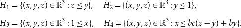 \begin{align*} H_1 &= \{(x,y,z) \in \mathbb{R}^3\;:\;z \leq y\}, \quad H_2 =\{(x,y,z) \in \mathbb{R}^3\;:\;y \leq 1\},\\[5pt] H_3 &= \{(x,y,z) \in \mathbb{R}^3\;:\;1 \leq x\}, \quad H_4 =\{(x,y,z) \in \mathbb{R}^3\;:\;x \leq bc(z-y)+by\}. \end{align*}
We see that
 \begin{align*} (1,1,1)&\in \partial H_1\cap \partial H_2 \cap \partial H_3 \cap \text{int}(H_4), \quad &&(b,1,1)\in \partial H_1\cap \partial H_2 \cap \text{int}(H_3) \cap \partial H_4\\[5pt] (1,1/b,1/b)&\in \partial H_1 \cap \text{int}(H_2) \cap \partial H_3 \cap \partial H_4, \quad &&(1,1,1-\frac{b-1}{bc})\in \text{int}(H_1)\cap \partial H_2 \cap \partial H_3 \cap \partial H_4. \end{align*}
Using Lemma 3.3 we can conclude that the last stated inclusion in the lemma indeed holds.
3.3 Proof of the Main Theorem
In this section we prove the Main Theorem. We utilize a number of inequalities for which the proofs can be found in the next section.
Lemma 3.7.
Let $q \in \{3,4\}$
,
$q \in \{3,4\}$
, $d \in \mathbb{Z}_{\geq 2}$
for
$d \in \mathbb{Z}_{\geq 2}$
for $q=3$
and
$q=3$
and $d \in \mathbb{Z}_{\geq 4}$
for
$d \in \mathbb{Z}_{\geq 4}$
for $q =4$
and let
$q =4$
and let $1- q/(d+1) \leq w \lt 1$
. Let
$1- q/(d+1) \leq w \lt 1$
. Let $a,b \in \mathbb{R}_{\gt 1}$
such that
$a,b \in \mathbb{R}_{\gt 1}$
such that
 \begin{equation} \max \!\left \{ b, \frac{b^d + w + k-2}{w b^d + (q-1)}\right \} \lt a \lt b^{\frac{b^d(q-1+w)(b-1)}{(b^d-1)(b-w)}}. \end{equation}
Then $F(\mathcal{T}_{a,b}) \subseteq \text{int}(\mathcal{T}_{a,b})$
.
$F(\mathcal{T}_{a,b}) \subseteq \text{int}(\mathcal{T}_{a,b})$
.
Proof. Recall from Section 2.2 that we can write $F$
as the composition
$F$
as the composition $G \circ P$
, where
$G \circ P$
, where $P(x_1,\ldots, x_{q-1}) = (x_1^d, \ldots, x_{q-1}^d)$
. In logarithmic coordinates the map
$P(x_1,\ldots, x_{q-1}) = (x_1^d, \ldots, x_{q-1}^d)$
. In logarithmic coordinates the map $\hat{P} = \log \circ P\circ \exp$
acts as multiplication by
$\hat{P} = \log \circ P\circ \exp$
acts as multiplication by $d$
. In the proof of Lemma 3.4 we showed that
$d$
. In the proof of Lemma 3.4 we showed that $\hat{\mathcal{T}}_{a,b}$
is a polytope whose vertices have entries
$\hat{\mathcal{T}}_{a,b}$
is a polytope whose vertices have entries $0$
,
$0$
, $\pm \hat{a}$
or
$\pm \hat{a}$
or $\pm \hat{b}$
. It follows that
$\pm \hat{b}$
. It follows that $\hat{P}(\hat{\mathcal{T}}_{a,b})$
is the same polytope where
$\hat{P}(\hat{\mathcal{T}}_{a,b})$
is the same polytope where $\hat{a}$
and
$\hat{a}$
and $\hat{b}$
are replaced by
$\hat{b}$
are replaced by $d\cdot \hat{a}$
and
$d\cdot \hat{a}$
and $d\cdot \hat{b}$
respectively. Because
$d\cdot \hat{b}$
respectively. Because $\hat{a} = \log\!(a)$
and
$\hat{a} = \log\!(a)$
and $\hat{b} = \log\!(b)$
, we can conclude that
$\hat{b} = \log\!(b)$
, we can conclude that $P(\mathcal{T}_{a,b}) = \mathcal{T}_{a^d,b^d}$
. It follows from Lemma 3.2 that it is enough to show that
$P(\mathcal{T}_{a,b}) = \mathcal{T}_{a^d,b^d}$
. It follows from Lemma 3.2 that it is enough to show that $G (\mathcal{T}_{a^d,b^d} \cap \mathcal{R}_{(123)}) = F(\mathcal{T}_{a,b} \cap \mathcal{R}_{(123)}) \subseteq \text{int}(\mathcal{T}_{a,b})$
for
$G (\mathcal{T}_{a^d,b^d} \cap \mathcal{R}_{(123)}) = F(\mathcal{T}_{a,b} \cap \mathcal{R}_{(123)}) \subseteq \text{int}(\mathcal{T}_{a,b})$
for $q=3$
and
$q=3$
and $G (\mathcal{T}_{a^d,b^d} \cap \mathcal{R}_{(134)}) = F(\mathcal{T}_{a,b} \cap \mathcal{R}_{(134)}) \subseteq \text{int}(\mathcal{T}_{a,b})$
for
$G (\mathcal{T}_{a^d,b^d} \cap \mathcal{R}_{(134)}) = F(\mathcal{T}_{a,b} \cap \mathcal{R}_{(134)}) \subseteq \text{int}(\mathcal{T}_{a,b})$
for $q=4$
.
$q=4$
.
We use Lemma 3.6 to conclude that it is enough to show that
 \begin{equation} G\big (\text{Conv}(\{(1,1),(b^d,1),(1,1-\frac{(b^d-1)\log\!(a)}{b^d\log\!(b)})\})\big ) \subseteq \text{int}(\mathcal{T}_{a,b}) \end{equation}
for $q=3$
and
$q=3$
and
 \begin{equation} G\big (\text{Conv}(\{(1,1,1),(b^d,1,1),(1,1/b^d,1/b^d),(1,1,1-\frac{(b^d-1)\log\!(a)}{b^d\log\!(b)})\})\big ) \subseteq \text{int}(\mathcal{T}_{a,b}) \end{equation}
for $q=4$
. We have to be careful here because initially we defined
$q=4$
. We have to be careful here because initially we defined $G$
as a map on
$G$
as a map on $\mathbb{R}_{\gt 0}^{q-1}$
. We can extend
$\mathbb{R}_{\gt 0}^{q-1}$
. We can extend $G$
to the half-space
$G$
to the half-space $H = \{(x_1, \ldots, x_{q-1})\;:\;x_1 + \cdots + x_{q-1} + w \gt 0\}$
. To show that the sets in equations (3.5) and (3.6) are contained in
$H = \{(x_1, \ldots, x_{q-1})\;:\;x_1 + \cdots + x_{q-1} + w \gt 0\}$
. To show that the sets in equations (3.5) and (3.6) are contained in $H$
it is enough to show that the vertices of these convex hulls are contained in
$H$
it is enough to show that the vertices of these convex hulls are contained in $H$
. This is clear for all but the last written vertex in either case. We will show that the equation
$H$
. This is clear for all but the last written vertex in either case. We will show that the equation $x_1 + \cdots + x_{q-1} + w \gt 0$
does indeed hold for these two points. Namely, by (3.4) we have
$x_1 + \cdots + x_{q-1} + w \gt 0$
does indeed hold for these two points. Namely, by (3.4) we have
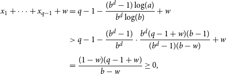 \begin{align*} x_1 + \cdots + x_{q-1} + w &= q-1 - \frac{(b^d-1)\log\!(a)}{b^d\log\!(b)} + w \\[5pt] & \gt q-1 - \frac{(b^d-1)}{b^d}\cdot \frac{b^d(q-1+w)(b-1)}{(b^d-1)(b-w)} + w\\[5pt] &= \frac{(1-w)(q-1+w)}{b-w} \geq 0, \end{align*}
as desired.
The map $G$
is a linear-fractional function, which means that
$G$
is a linear-fractional function, which means that $G$
sends line segments to line segments (see e.g. Section 2.3.3 of [Reference Boyd and Vandenberghe6]). Thus, for any set of points
$G$
sends line segments to line segments (see e.g. Section 2.3.3 of [Reference Boyd and Vandenberghe6]). Thus, for any set of points $p_1, \ldots, p_n$
we have
$p_1, \ldots, p_n$
we have $G(\text{Conv}(\{p_1,\ldots, p_n\})) = \text{Conv}{(\{G(p_1),\ldots,G(p_n)\})}$
. Let
$G(\text{Conv}(\{p_1,\ldots, p_n\})) = \text{Conv}{(\{G(p_1),\ldots,G(p_n)\})}$
. Let
 \begin{equation*} f_{q}(x) = \frac {w x + q-1}{x + k-2 + w} \quad \text { and }\quad g(x) = \frac {(1+w)x+2}{2x+1+w}. \end{equation*}
The left-hand side of (15) is equal to
 \begin{equation*} \text {Conv}\!\left (\{(1,1),(f_3(b^d),1),(1,f_{3}\left (1-\frac {(b^d-1)\log\!(a)}{b^d\log\!(b)}\right ))\}\right ) \end{equation*}
and the left-hand side of (16) is equal to
 \begin{equation*} \text {Conv}(\{(1,1,1),(f_4(b^d),1,1),(1,g(1/b^d),g(1/b^d)),(1,1,f_4\left (1-\frac {(b^d-1)\log\!(a)}{b^d\log\!(b)}\right )). \end{equation*}
We can use Lemma 3.6 to see that it is enough to show that
 \begin{equation} f_q(b^d) \gt 1/a, \quad g(1/b^d) \lt b \quad \text{ and } \quad f_q\left (1-\frac{(b^d-1)\log\!(a)}{b^d\log\!(b)}\right ) \lt b \end{equation}
to conclude that these sets are contained in $\mathcal{T}_{a,b} \cap \mathcal{R}_{(23)}$
and
$\mathcal{T}_{a,b} \cap \mathcal{R}_{(23)}$
and $\mathcal{T}_{a,b} \cap \mathcal{R}_{(243)}$
respectively. The first inequality follows directly from the assumptions. The second inequality follows from item (4) of Theorem 4.1 below. For the last inequality we note that
$\mathcal{T}_{a,b} \cap \mathcal{R}_{(243)}$
respectively. The first inequality follows directly from the assumptions. The second inequality follows from item (4) of Theorem 4.1 below. For the last inequality we note that $f_q$
is strictly decreasing and
$f_q$
is strictly decreasing and $1-\frac{(b^d-1)\log\!(a)}{b^d\log\!(b)}$
is also strictly decreasing in
$1-\frac{(b^d-1)\log\!(a)}{b^d\log\!(b)}$
is also strictly decreasing in $a$
. Therefore, it is enough to show the inequality for
$a$
. Therefore, it is enough to show the inequality for $a= b^{\frac{b^d(q-1+w)(b-1)}{(b^d-1)(b-w)}}$
. We obtain
$a= b^{\frac{b^d(q-1+w)(b-1)}{(b^d-1)(b-w)}}$
. We obtain
 \begin{equation*} f_q\left (1-\frac {(b^d-1)\log\!(a)}{b^d\log\!(b)}\right ) \lt f_q\left (1-\frac {(q-1+w)(b-1)}{b-w}\right ) = b. \end{equation*}
Because the inequalities in (17) are strict we can even conclude that $\mathcal{T}_{a,b}$
gets mapped strictly inside itself by
$\mathcal{T}_{a,b}$
gets mapped strictly inside itself by $F$
, i.e.
$F$
, i.e. $F(\mathcal{T}_{a,b}) \subseteq \text{int}(\mathcal{T}_{a,b})$
.
$F(\mathcal{T}_{a,b}) \subseteq \text{int}(\mathcal{T}_{a,b})$
.
Theorem 3.8.
Let $q \in \{3,4\}$
,
$q \in \{3,4\}$
, $d \in \mathbb{Z}_{\geq 2}$
for
$d \in \mathbb{Z}_{\geq 2}$
for $q=3$
and
$q=3$
and $d \in \mathbb{Z}_{\geq 4}$
for
$d \in \mathbb{Z}_{\geq 4}$
for $q =4$
and let
$q =4$
and let $1- q/(d+1) \leq w \lt 1$
with
$1- q/(d+1) \leq w \lt 1$
with $w\gt 0$
. Then the
$w\gt 0$
. Then the $q$
-state Potts model with weight
$q$
-state Potts model with weight $w$
on the infinite
$w$
on the infinite $(d+1)$
-regular tree,
$(d+1)$
-regular tree, $\mathbb{T}_d$
, has a unique Gibbs measure.
$\mathbb{T}_d$
, has a unique Gibbs measure.
Proof. We will construct a sequence of subsets $\{\mathcal{T}_n\}_{n\geq 0}$
as is described in Lemma 2.3. Define the functions
$\{\mathcal{T}_n\}_{n\geq 0}$
as is described in Lemma 2.3. Define the functions
 \begin{equation*} L(b) = \max \!\left \{b, \frac {b^d + w + k-2}{w b^d + (q-1)}\right \} \quad \text { and }\quad U(b) = \min \!\left \{b^2,b^{\frac {b^d(q-1+w)(b-1)}{(b^d-1)(b-w)}}\right \}. \end{equation*}
It follows from items (1), (2) and (3) of Theorem 4.1 that $L(b) \lt U(b)$
for
$L(b) \lt U(b)$
for $b \gt 1$
. We define
$b \gt 1$
. We define $M(b) = (L(b)+U(b))/2$
and note that
$M(b) = (L(b)+U(b))/2$
and note that $L(b) \lt M(b) \lt U(b)$
for
$L(b) \lt M(b) \lt U(b)$
for $b\gt 1$
. Any element of
$b\gt 1$
. Any element of $\mathbb{R}_{\gt 0}^{q-1}$
is contained in
$\mathbb{R}_{\gt 0}^{q-1}$
is contained in $\mathcal{T}_{b,b}$
for a large enough value of
$\mathcal{T}_{b,b}$
for a large enough value of $b$
. It follows that we can choose
$b$
. It follows that we can choose $b_0\gt 1$
such that
$b_0\gt 1$
such that $\mathcal{T}_{b_0,b_0}$
contains both the vector with every entry equal to
$\mathcal{T}_{b_0,b_0}$
contains both the vector with every entry equal to $1/w$
and the vectors obtained from the all-ones vector with a single entry changed to
$1/w$
and the vectors obtained from the all-ones vector with a single entry changed to $w$
. Because
$w$
. Because $M(b_0)\gt b_0$
we have
$M(b_0)\gt b_0$
we have $\mathcal{T}_{b_0,b_0} \subset \mathcal{T}_{M(b_0),b_0}$
and thus
$\mathcal{T}_{b_0,b_0} \subset \mathcal{T}_{M(b_0),b_0}$
and thus $\mathcal{T}_{M(b_0),b_0}$
contains these vectors too. Inductively we now define
$\mathcal{T}_{M(b_0),b_0}$
contains these vectors too. Inductively we now define $b_n$
for
$b_n$
for $n\geq 1$
by
$n\geq 1$
by
 \begin{equation*} b_n = \inf \left \{b\;:\;F(\mathcal {T}_{M(b_{n-1}),b_{n-1}}) \subseteq \mathcal {T}_{M(b),b}\right \}. \end{equation*}
Because $\mathcal{T}_{M(b),b}$
moves continuously with
$\mathcal{T}_{M(b),b}$
moves continuously with $b$
it follows from Lemma 3.7 that
$b$
it follows from Lemma 3.7 that $\{b_n\}_{n \geq 1}$
is a strictly decreasing sequence. The sequence is clearly bounded below by
$\{b_n\}_{n \geq 1}$
is a strictly decreasing sequence. The sequence is clearly bounded below by $1$
and thus it must have a limit. We claim that this limit is
$1$
and thus it must have a limit. We claim that this limit is $1$
. For the sake of contradiction assume that it has a limit
$1$
. For the sake of contradiction assume that it has a limit $b_\infty \gt 1$
. The set
$b_\infty \gt 1$
. The set $\mathcal{T}_{M(b_\infty ),b_\infty }$
gets mapped strictly inside itself by
$\mathcal{T}_{M(b_\infty ),b_\infty }$
gets mapped strictly inside itself by $F$
and thus there is a
$F$
and thus there is a $b'\lt b_\infty$
such that
$b'\lt b_\infty$
such that $\mathcal{T}_{M(b_\infty ),b_\infty }$
also gets mapped strictly inside
$\mathcal{T}_{M(b_\infty ),b_\infty }$
also gets mapped strictly inside $\mathcal{T}_{M(b'),b'}$
. This is an open condition, so there is an
$\mathcal{T}_{M(b'),b'}$
. This is an open condition, so there is an $\epsilon \gt 0$
such that
$\epsilon \gt 0$
such that $\mathcal{T}_{M(b),b}$
gets mapped strictly inside
$\mathcal{T}_{M(b),b}$
gets mapped strictly inside $\mathcal{T}_{M(b'),b'}$
for all
$\mathcal{T}_{M(b'),b'}$
for all $b \in [b_\infty,b_\infty + \epsilon )$
. There must be an integer
$b \in [b_\infty,b_\infty + \epsilon )$
. There must be an integer $N$
such that
$N$
such that $b_N \in [b_\infty,b_\infty + \epsilon )$
, but then
$b_N \in [b_\infty,b_\infty + \epsilon )$
, but then $b_{N+1} \lt b' \lt b_\infty$
, so
$b_{N+1} \lt b' \lt b_\infty$
, so $b_\infty$
cannot be the limit of the decreasing sequence
$b_\infty$
cannot be the limit of the decreasing sequence $\{b_n\}_{n \geq 0}$
.
$\{b_n\}_{n \geq 0}$
.
We define $\mathcal{T}_n = \mathcal{T}_{M(b_n),b_n}$
. We have
$\mathcal{T}_n = \mathcal{T}_{M(b_n),b_n}$
. We have $b \lt M(b) \lt b^2$
, so it follows from Lemma 3.4 that every
$b \lt M(b) \lt b^2$
, so it follows from Lemma 3.4 that every $\mathcal{T}_n$
is log-convex. We have chosen
$\mathcal{T}_n$
is log-convex. We have chosen $\mathcal{T}_0$
such that condition (1) of Lemma 2.3 is satisfied. By construction
$\mathcal{T}_0$
such that condition (1) of Lemma 2.3 is satisfied. By construction $F(\mathcal{T}_{m}) \subseteq \mathcal{T}_{m+1}$
for all
$F(\mathcal{T}_{m}) \subseteq \mathcal{T}_{m+1}$
for all $m$
and thus condition (2) of Lemma 2.3 is satisfied. Finally, because both
$m$
and thus condition (2) of Lemma 2.3 is satisfied. Finally, because both $b_n$
and
$b_n$
and $M(b_n)$
converge to
$M(b_n)$
converge to $1$
, it follows that the sequence of sets
$1$
, it follows that the sequence of sets $\mathcal{T}_n$
converges to the set consisting of just the all-ones vector. This means that condition (3) of Lemma 2.3 is satisfied. We can conclude that
$\mathcal{T}_n$
converges to the set consisting of just the all-ones vector. This means that condition (3) of Lemma 2.3 is satisfied. We can conclude that $\mathbb{T}_d$
has a unique Gibbs measure.
$\mathbb{T}_d$
has a unique Gibbs measure.
Remark 3.9. The assumption $w\gt 0$
is critical in the case
$w\gt 0$
is critical in the case $q=3$
and
$q=3$
and $d=2$
, as it is well known there are multiple Gibbs measures at
$d=2$
, as it is well known there are multiple Gibbs measures at $w_c=0$
when
$w_c=0$
when $q=d+1$
. One sees this in our argument as well. For the base case of the induction, condition (1) of Lemma 2.3, we need
$q=d+1$
. One sees this in our argument as well. For the base case of the induction, condition (1) of Lemma 2.3, we need $\mathcal{T}_0$
to contain the vectors
$\mathcal{T}_0$
to contain the vectors $(1,w) =(1,0)$
,
$(1,w) =(1,0)$
, $(w,1)=(0,1)$
and
$(w,1)=(0,1)$
and $(1/w,1/w) = (\infty,\infty )$
. If we take the log convex hull of these vectors and apply
$(1/w,1/w) = (\infty,\infty )$
. If we take the log convex hull of these vectors and apply $F$
, we obtain a region that again contains the vectors
$F$
, we obtain a region that again contains the vectors $(1,w) =(1,0)$
,
$(1,w) =(1,0)$
, $(w,1)=(0,1)$
and
$(w,1)=(0,1)$
and $(1/w,1/w) = (\infty,\infty )$
. It is thus possible to choose boundary conditions that yield unbounded ratios at an arbitrary distance from the leaves. This observation is closely related to the existence of so-called frozen colourings [Reference Brightwell and Winkler5]. These give distinct trivial Gibbs measures, each supported on a single colouring of
$(1/w,1/w) = (\infty,\infty )$
. It is thus possible to choose boundary conditions that yield unbounded ratios at an arbitrary distance from the leaves. This observation is closely related to the existence of so-called frozen colourings [Reference Brightwell and Winkler5]. These give distinct trivial Gibbs measures, each supported on a single colouring of $\mathbb{T}_2$
.
$\mathbb{T}_2$
.
4. Proof of the inequalities
This section is dedicated to showing all the inequalities from the previous section are satisfied. We define the following functions
 \begin{align*} l(q,d,w,b) &= \frac{ b^d+q-2+w}{w b^d + q-1}, \quad &&g(d,w,b) = \frac{2b^d+1+w}{(1+w)b^d+2},\\[5pt] h(q,d,w,b) &=\frac{ b^d (b-1)(q-1+w)}{\!\left (b^d-1\right ) (b - w)}, \quad \quad &&u(q,d,w,b) = b^{h(q,d,w,b)}. \end{align*}
We mostly consider these as functions in $b$
and consider only
$b$
and consider only $b \geq 1$
. Note that
$b \geq 1$
. Note that $h(q,d,w,b)$
has a removable singularity in
$h(q,d,w,b)$
has a removable singularity in $b=1$
with
$b=1$
with $h(q,d,w,1) = \frac{q-1+w}{d(1-w)}$
. The main theorem we prove in this section is the following.
$h(q,d,w,1) = \frac{q-1+w}{d(1-w)}$
. The main theorem we prove in this section is the following.
Theorem 4.1.
For $q=3, d \geq 2$
and
$q=3, d \geq 2$
and $w \in [1 - \frac{3}{d+1}, 1)$
or for
$w \in [1 - \frac{3}{d+1}, 1)$
or for $q=4, d \geq 4$
and
$q=4, d \geq 4$
and $w \in [1 - \frac{4}{d+1}, 1)$
we have for each
$w \in [1 - \frac{4}{d+1}, 1)$
we have for each $b \gt 1$
-
(1)
$u(q,d,w,b) \gt l(q,d,w,b)$
, -
(2)
$u(q,d,w,b) \gt b$
, -
(3)
$b^2\gt l(q,d,w,b)$
.


And for all $b \gt 1$
and
$b \gt 1$
and $d \geq 3$
and
$d \geq 3$
and $w \in [1 - \frac{4}{d+1}, 1)$
we have
$w \in [1 - \frac{4}{d+1}, 1)$
we have
-
(4)
$g(d,w,b) \lt b$
.

In the next section we show it is enough to prove Theorem 4.1 holds for $w = w_c = 1 - \frac{q}{d+1}$
where we take
$w = w_c = 1 - \frac{q}{d+1}$
where we take $q=4$
in inequality (4). Subsequently, inequality (2) is proved in Corollary 4.5, inequality (3) is proved in Lemma 4.6 and inequality (4) is proved in Lemma 4.3. The proof of inequality (1) is the most involved and is the result of Lemmas 4.7 and 4.8.
$q=4$
in inequality (4). Subsequently, inequality (2) is proved in Corollary 4.5, inequality (3) is proved in Lemma 4.6 and inequality (4) is proved in Lemma 4.3. The proof of inequality (1) is the most involved and is the result of Lemmas 4.7 and 4.8.
4.1 Reduction to
$w = w_c$

Lemma 4.2.
Let $q \geq 2, d \geq 1$
and
$q \geq 2, d \geq 1$
and $w \in [0,1)$
. For
$w \in [0,1)$
. For $b\gt 1$
we have
$b\gt 1$
we have $l(q,d,w,b)$
and
$l(q,d,w,b)$
and $g(d,w,b)$
are decreasing in
$g(d,w,b)$
are decreasing in $w$
, while
$w$
, while $u(q,d,w,b)$
is increasing in
$u(q,d,w,b)$
is increasing in $w$
.
$w$
.
Proof. We compute
 \begin{align*} \frac{\partial }{\partial w} l(q,d,w,b)&= - \frac{(b^d-1)(b^d+q-1)}{(wb^d+q-1)^2},\\[5pt] \frac{\partial }{\partial w} g(d,w,b) &= -\frac{2(b^{2d}-1)}{((1+w)b^d+2)^2},\\[5pt] \frac{\partial }{\partial w} u(q,d,w,b) &=u(q,d,w,b) \cdot \frac{b^d(b-1)(b+q-1)\log{b}}{(b^d-1)(b-w)^2}. \end{align*}
We see that for $b\gt 1$
we have
$b\gt 1$
we have $\frac{\partial }{\partial w} l(q,d,w,b)\lt 0$
,
$\frac{\partial }{\partial w} l(q,d,w,b)\lt 0$
, $\frac{\partial }{\partial w} g(d,w,b) \lt 0$
and
$\frac{\partial }{\partial w} g(d,w,b) \lt 0$
and $\frac{\partial }{\partial w} u(q,d,w,b)\gt 0$
, so the lemma follows.
$\frac{\partial }{\partial w} u(q,d,w,b)\gt 0$
, so the lemma follows.
From Lemma 4.2 it follows that if we can show Theorem 4.1 holds for $w = w_c$
, then it also holds for all
$w = w_c$
, then it also holds for all $ w\in [w_c,1)$
. So from now on we will work with
$ w\in [w_c,1)$
. So from now on we will work with $l(b,w_c,d,q)$
,
$l(b,w_c,d,q)$
, $u(b,w_c,d,q)$
and
$u(b,w_c,d,q)$
and $h(b,w_c,d)$
. To shorten notation we write
$h(b,w_c,d)$
. To shorten notation we write
 \begin{align*} l(b) &= \frac{(d+1) b^d+d(q-1)-1}{(d-q+1) b^d+(d+1) (q-1)}, \quad &&g(b) = \frac{(d+1)b^d + d-1}{(d-1)b^d+d+1},\\[5pt] h(b) &=\frac{d q b^d (b-1)}{\left (b^d-1\right ) ((d+1)(b-1)+q)},\quad &&u(b) = b^{h(b)}. \end{align*}
We note that the function $h$
has a removable singularity in
$h$
has a removable singularity in $1$
with
$1$
with $h(1)=1$
.
$h(1)=1$
.
4.2 Inequalities
$g(b) \lt b$
,
$u(b) \gt b$
and
$b^2 \gt l(b)$


We will start by showing $g(b) \lt b$
holds for
$g(b) \lt b$
holds for $b \gt 1$
and
$b \gt 1$
and $d \geq 2$
.
$d \geq 2$
.
Lemma 4.3.
Let $d \geq 2$
and
$d \geq 2$
and $b\gt 1$
. Then we have
$b\gt 1$
. Then we have $ g(b) \lt b.$
Proof. We have $g(1) = 1$
and
$g(1) = 1$
and $g'(1) = 1$
. Furthermore, one can see
$g'(1) = 1$
. Furthermore, one can see
 \begin{equation*} g''(b) = -\frac {4 d^2 \!\left (d^2-1\right )\! \left (b^d-1\right ) b^{d-2}}{\!\left ((d-1) b^d+d+1\right )^3} \lt 0 \end{equation*}
for $d \geq 2$
and
$d \geq 2$
and $b \gt 1$
. This implies
$b \gt 1$
. This implies $g(b) \lt b$
for
$g(b) \lt b$
for $d \geq 2$
and
$d \geq 2$
and $b \gt 1$
.
$b \gt 1$
.
Next we show that $h$
is increasing in
$h$
is increasing in $b$
. This fact will immediately give us inequality (2). Furthermore, it is also helpful in proving a sufficient condition for inequality (1) to hold, see Lemma 4.7 below.
$b$
. This fact will immediately give us inequality (2). Furthermore, it is also helpful in proving a sufficient condition for inequality (1) to hold, see Lemma 4.7 below.
Lemma 4.4.
For all $b \gt 1,d\geq 2$
and
$b \gt 1,d\geq 2$
and $q \geq 2$
we have
$q \geq 2$
we have $h'(b)\gt 0$
.
$h'(b)\gt 0$
.
Proof. We compute
 \begin{equation*} h'(b)= \frac {k d b^{d-1} \!\left (q b^{d+1}- d\!\left (d+1\right )\!b^2+ \left (2 d^2-d q+2 d-q\right )\!b-d^2+d q-d\right )}{\left (b^d-1\right )^2 \!((d+1)(b-1)+q)^2}. \end{equation*}
It suffices to show that
 \begin{equation*} m(b) \;:\!=\; q b^{d+1}- d\!\left (d+1\right )\!b^2+ \left (2 d^2-d q+2 d-q\right )\!b-d^2+d q-d \end{equation*}
is positive for $b\gt 1$
. We compute
$b\gt 1$
. We compute
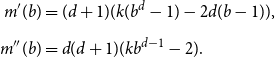 \begin{align*} m'(b) &= (d+1)(k(b^d-1)-2d(b-1)),\\[5pt] m''(b) &= d(d+1)(kb^{d-1}-2). \end{align*}
We see $m''(b) \gt 0$
for
$m''(b) \gt 0$
for $b \gt 1,d\geq 2$
and
$b \gt 1,d\geq 2$
and $q \geq 2$
. Noting that
$q \geq 2$
. Noting that $m'(1) = 0$
and
$m'(1) = 0$
and $m(1) = 0$
, it follows that
$m(1) = 0$
, it follows that $m'(b)$
and
$m'(b)$
and $m(b)$
are strictly positive for
$m(b)$
are strictly positive for $b\gt 1$
.
$b\gt 1$
.
This immediately implies inequality (2).
Corollary 4.5.
For $b\gt 1$
we have
$b\gt 1$
we have $u(b) \gt b$
.
$u(b) \gt b$
.
Proof. Recall $u(b) = b^{h(b)}$
. As
$u(b) = b^{h(b)}$
. As $h(1) = 1$
and
$h(1) = 1$
and $h'(b)\gt 0$
for
$h'(b)\gt 0$
for $b \gt 1$
by Lemma 4.4, we see
$b \gt 1$
by Lemma 4.4, we see $u(b) \gt b$
for
$u(b) \gt b$
for $b \gt 1$
follows.
$b \gt 1$
follows.
Until this point, we did not need to assume $q=3$
or
$q=3$
or $q=4$
for the computations to work, but for inequality (3) to hold we do need some restrictions on
$q=4$
for the computations to work, but for inequality (3) to hold we do need some restrictions on $q$
and
$q$
and $d$
.
$d$
.
Lemma 4.6.
For $q=3$
and
$q=3$
and $d \geq 2$
and for
$d \geq 2$
and for $q = 4$
and
$q = 4$
and $d \geq 4$
we have
$d \geq 4$
we have $ l(b) \lt b^2,$
for all
$ l(b) \lt b^2,$
for all $b\gt 1$
.
$b\gt 1$
.
Proof. Multiplying both sides of the inequality with the positive factor $(d-q+1)b^d+(d+1) (q-1)$
we obtain the equivalent inequality
$(d-q+1)b^d+(d+1) (q-1)$
we obtain the equivalent inequality
 \begin{equation*} (d+1) b^d+d(q-1)-1 \lt (d-q+1)b^{d+2} +(d+1) (q-1)b^2. \end{equation*}
To show that this inequality holds we show that the polynomial
 \begin{equation*} Q(b) = (d-q+1)b^{d+2} - (d+1)b^d +(d+1) (q-1)b^2- d(q-1) + 1 \end{equation*}
is strictly positive for $b\gt 1$
. For
$b\gt 1$
. For $d\geq 2$
we compute
$d\geq 2$
we compute
 \begin{align*} Q'(b) &= (d+2)(d-q+1)b^{d+1} - (d+1)db^{d-1} +2(d+1)(q-1)b,\\[5pt] Q''(b) &= (d+2)(d+1)(d-q+1)b^{d} - (d+1)d(d-1)b^{d-2} +2(d+1)(q-1),\\[5pt] Q'''(b) &=d(d+1)b^{d-3} \left ((d+2)(d-q+1)b^2 - (d-1)(d-2) \right ), \end{align*}
Because $d+1 \geq k$
we find that for all
$d+1 \geq k$
we find that for all $b \geq 1$
 \begin{equation*} (d+2)(d-q+1)b^2 - (d-1)(d-2) \geq (d+2)(d-q+1) - (d-1)(d-2) = (6-q)d - 2q. \end{equation*}
For $q=3$
this quantity is nonnegative for
$q=3$
this quantity is nonnegative for $d \geq 2$
and for
$d \geq 2$
and for $q=4$
this quantity is nonnegative for
$q=4$
this quantity is nonnegative for $d \geq 4$
. So in our case we can conclude that
$d \geq 4$
. So in our case we can conclude that $Q'''(b) \geq 0$
for all
$Q'''(b) \geq 0$
for all $b \geq 1$
. As we have
$b \geq 1$
. As we have $Q''(1) = d(d+1) \gt 0$
,
$Q''(1) = d(d+1) \gt 0$
, $Q'(1) = 3d\gt 0$
and
$Q'(1) = 3d\gt 0$
and $Q(1) = 0$
, it follows that
$Q(1) = 0$
, it follows that $Q''(b),Q'(b)$
and
$Q''(b),Q'(b)$
and $Q(b)$
are strictly positive for
$Q(b)$
are strictly positive for $b\gt 1$
.
$b\gt 1$
.
4.3 The inequality
$u(b) \gt l(b)$

The following lemma contains a sufficient condition to prove this inequality. In the remainder of the section we prove that this condition is satisfied.
Lemma 4.7.
Suppose for all $b\gt 1$
we have
$b\gt 1$
we have
 \begin{equation} \frac{l'(b)}{l(b)} \lt \frac{h(b)}{b} + 2\frac{b-1}{b+1}g'(b). \end{equation}
Then $u(b) \gt l(b)$
for all
$u(b) \gt l(b)$
for all $b \gt 1$
.
$b \gt 1$
.
Proof. As $l(b)$
and
$l(b)$
and $u(b)$
are strictly positive for
$u(b)$
are strictly positive for $b \geq 1$
, we can define
$b \geq 1$
, we can define
 \begin{equation*} F(b) = \log\!(u(b))-\log\!(l(b)) \end{equation*}
for $b \geq 1$
. Then we have
$b \geq 1$
. Then we have
 \begin{equation*} F'(b) = \frac {u'(b)}{u(b)} - \frac {l'(b)}{l(b)} = \frac {h(b)}{b} + \log\!(b) h'(b) - \frac {l'(b)}{l(b)}. \end{equation*}
For $b\gt 1$
we have that
$b\gt 1$
we have that $h'(b)\gt 0$
by Lemma 4.4 and
$h'(b)\gt 0$
by Lemma 4.4 and $\log\!(b) \gt 2(b-1)/(b+1)$
, therefore
$\log\!(b) \gt 2(b-1)/(b+1)$
, therefore
 \begin{equation*} F'(b) \gt \frac {h(b)}{b} + 2\frac {b-1}{b+1} h'(b) - \frac {l'(b)}{l(b)}, \end{equation*}
which is positive by (18). It is easy to see $F'(1) = 0$
. Hence
$F'(1) = 0$
. Hence $F$
has a global minimum in
$F$
has a global minimum in $b=1$
. As
$b=1$
. As $F(1) = 0$
, it follows that
$F(1) = 0$
, it follows that $u(b) \gt l(b)$
for all
$u(b) \gt l(b)$
for all $b \gt 1$
, which is what we wanted to show.
$b \gt 1$
, which is what we wanted to show.
This lemma is useful because proving the inequality $u(b) \gt l(b)$
for all
$u(b) \gt l(b)$
for all $b \gt 1$
can now be reduced to proving inequalities involving rational functions and with some work to inequalities involving only polynomials. The next lemma shows that (18) holds. For this to work we do need to restrict to
$b \gt 1$
can now be reduced to proving inequalities involving rational functions and with some work to inequalities involving only polynomials. The next lemma shows that (18) holds. For this to work we do need to restrict to $q=3$
and
$q=3$
and $d \geq 2$
or
$d \geq 2$
or $q=4$
and
$q=4$
and $d \geq 4$
.
$d \geq 4$
.
Lemma 4.8.
For $q=3$
and
$q=3$
and $d\geq 2$
and for
$d\geq 2$
and for $q=4$
and
$q=4$
and $d\geq 4$
and any
$d\geq 4$
and any $b\gt 1$
we have
$b\gt 1$
we have
 \begin{equation*} \frac {l'(b)}{l(b)} \lt \frac {h(b)}{b} + 2\frac {b-1}{b+1}h'(b). \end{equation*}
Proof. We introduce the following polynomials
 \begin{align*} p(b) &= (d+1) b^d+d(q-1)-1, \quad &&q(b) = (d-q+1) b^d+(d+1) (q-1),\\[5pt] s(b) &= d q b^d (b-1), \quad &&t(b) = \left (b^d-1\right ) ((d+1)(b-1)+q). \end{align*}
Thus, $l(b) = p(b)/q(b)$
and
$l(b) = p(b)/q(b)$
and $h(b)=s(b)/t(b)$
. Furthermore, we define
$h(b)=s(b)/t(b)$
. Furthermore, we define $r(b) = q(b)p'(b) - p(b)q'(b)$
and
$r(b) = q(b)p'(b) - p(b)q'(b)$
and $v(b) = t(b)s'(b)-s(b)t'(b)$
. It is worth noting that
$v(b) = t(b)s'(b)-s(b)t'(b)$
. It is worth noting that $r(b)$
simplifies to
$r(b)$
simplifies to $q^2 d^2 b^{d-1}$
. The inequality we want to prove can now be written as
$q^2 d^2 b^{d-1}$
. The inequality we want to prove can now be written as
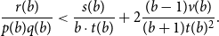 \begin{equation*} \frac {r(b)}{p(b)q(b)} \lt \frac {s(b)}{b \cdot t(b)} + 2 \frac {(b-1)v(b)}{(b+1)t(b)^2}. \end{equation*}
For $b \gt 1$
the quantity
$b \gt 1$
the quantity $b(b+1)p(b)q(b)t(b)^2$
is strictly positive and thus it is equivalent to prove the inequality, where we have multiplied both sides by this term. We see that it is enough to prove that the following polynomial is strictly positive for all
$b(b+1)p(b)q(b)t(b)^2$
is strictly positive and thus it is equivalent to prove the inequality, where we have multiplied both sides by this term. We see that it is enough to prove that the following polynomial is strictly positive for all $b\gt 1$
 \begin{equation} P(b) = (b+1)s(b)p(b)q(b)t(b) + 2b(b-1)v(b)p(b)q(b) - b(b+1)r(b)t(b)^2. \end{equation}
It can be checked that the terms $s(b)$
,
$s(b)$
, $b\cdot v(b)$
and
$b\cdot v(b)$
and $b\cdot r(b)$
all contain a factor
$b\cdot r(b)$
all contain a factor $qdb^d$
and thus
$qdb^d$
and thus $P_0(b) = P(b)/(kdb^d)$
is a polynomial in
$P_0(b) = P(b)/(kdb^d)$
is a polynomial in $b$
whose coefficients are polynomials in
$b$
whose coefficients are polynomials in $d$
. The remainder of the proof will be dedicated to showing that
$d$
. The remainder of the proof will be dedicated to showing that $P_0(b)$
is strictly positive for
$P_0(b)$
is strictly positive for $b\gt 1$
.
$b\gt 1$
.
To avoid ambiguity later, we prove this for $q=3$
in the two cases
$q=3$
in the two cases $d=2$
and
$d=2$
and $d=3$
separately. For
$d=3$
separately. For $d=2$
we have
$d=2$
we have
 \begin{equation*} P_0(b) = 54 (b-1)^6+54 (b-1)^5 \end{equation*}
and for $d=3$
we have
$d=3$
we have
 \begin{align*} P_0(b) =& 16 (b-1)^{12}+212 (b-1)^{11}+1236 (b-1)^{10}+4116 (b-1)^9+8793 (b-1)^8 \\[5pt] &\quad +12789 (b-1)^7+12123 (b-1)^6+6318 (b-1)^5+1458 (b-1)^4. \end{align*}
In both cases all the coefficients of $P_0(b)$
are strictly positive when written as a polynomial in
$P_0(b)$
are strictly positive when written as a polynomial in $b-1$
and thus the polynomials are strictly positive for
$b-1$
and thus the polynomials are strictly positive for $b\gt 1$
.
$b\gt 1$
.
We will now assume that $d \geq 4$
. It can be seen by cross-multiplying the terms in the individual polynomials in (19) that the only coefficients of
$d \geq 4$
. It can be seen by cross-multiplying the terms in the individual polynomials in (19) that the only coefficients of $P_0(b)$
that can be non-zero appear in the
$P_0(b)$
that can be non-zero appear in the $b^{i\cdot d+j}$
terms where
$b^{i\cdot d+j}$
terms where $i,j \in \{0,1,2,3\}$
. The exact coefficients are recorded in Table 1. For
$i,j \in \{0,1,2,3\}$
. The exact coefficients are recorded in Table 1. For $n \in \{1,2,3\}$
we inductively define the polynomials
$n \in \{1,2,3\}$
we inductively define the polynomials $P_n(b) = P_{n-1}^{(4)}(b)/b^{d-4}$
. Note that in this way
$P_n(b) = P_{n-1}^{(4)}(b)/b^{d-4}$
. Note that in this way $P_n(b)$
is a polynomial whose only non-zero coefficients appear in the
$P_n(b)$
is a polynomial whose only non-zero coefficients appear in the $b^{i\cdot d + j}$
term, where
$b^{i\cdot d + j}$
term, where $0\leq i \leq 3-n$
and
$0\leq i \leq 3-n$
and $j \in \{0,1,2,3\}$
.
$j \in \{0,1,2,3\}$
.
Table 1 The coefficients of $P_0(b)$
for
$P_0(b)$
for $d\geq 4$
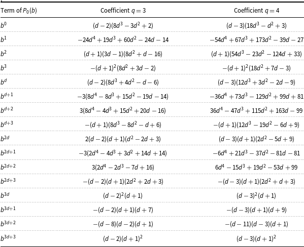
Table 2 The values of $P_j^{(i)}(1)$
for
$P_j^{(i)}(1)$
for $q=3$
in the variable
$q=3$
in the variable $x=d-4$
divided by
$x=d-4$
divided by $6 (x+4)^3 (x+5)$
for
$6 (x+4)^3 (x+5)$
for $i,j \in \{0,1,2,3\}$
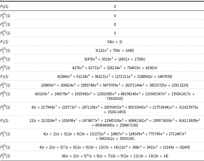
Table 3 The values of $P_j^{(i)}(1)$
for
$P_j^{(i)}(1)$
for $q=4$
in the variable
$q=4$
in the variable $x=d-4$
divided by
$x=d-4$
divided by $8 (x+4)^3 (x+5)$
for
$8 (x+4)^3 (x+5)$
for $i,j \in \{0,1,2,3\}$
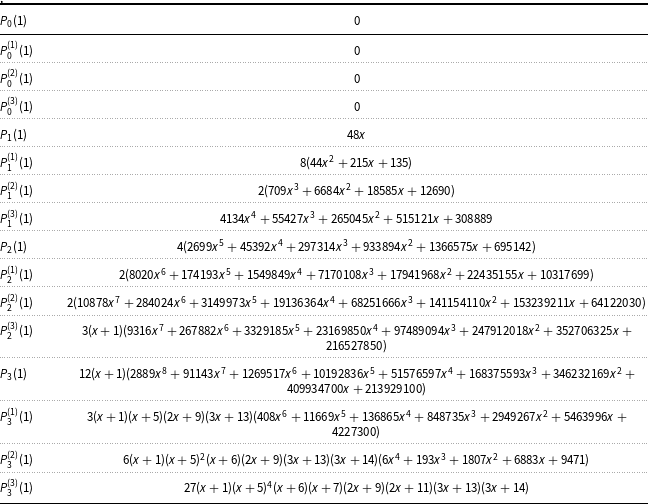
The values of $P_{j}^{(i)}(1)$
as a polynomial in
$P_{j}^{(i)}(1)$
as a polynomial in $x = d-4$
, up to a common positive multiplicative factor, for
$x = d-4$
, up to a common positive multiplicative factor, for $q=3$
and
$q=3$
and $q=4$
are contained in Tables 2 and 3 respectively. These polynomials have only nonnegative coefficients, from which it follows that their values are nonnegative for all
$q=4$
are contained in Tables 2 and 3 respectively. These polynomials have only nonnegative coefficients, from which it follows that their values are nonnegative for all $d\geq 4$
.
$d\geq 4$
.
The polynomial $P_3(b)$
is a cubic polynomial and thus its third derivative
$P_3(b)$
is a cubic polynomial and thus its third derivative $P_3^{(3)}(b)$
is constant. Its exact value, which is recorded in Table 2 for
$P_3^{(3)}(b)$
is constant. Its exact value, which is recorded in Table 2 for $q=3$
and in Table 3 for
$q=3$
and in Table 3 for $q=4$
, is strictly positive for all
$q=4$
, is strictly positive for all $x \geq 0$
, i.e. for all
$x \geq 0$
, i.e. for all $d \geq 4$
. We claim that it now follows inductively that
$d \geq 4$
. We claim that it now follows inductively that $P_j^{(i)}(b)$
is strictly positive for all
$P_j^{(i)}(b)$
is strictly positive for all $b \gt 1$
. Namely, suppose that for
$b \gt 1$
. Namely, suppose that for $i\in \{0,1,2,3\}$
we have shown that
$i\in \{0,1,2,3\}$
we have shown that $P_{j}^{(i+1)}(b)$
is strictly positive for
$P_{j}^{(i+1)}(b)$
is strictly positive for $b\gt 1$
. Then it follows that
$b\gt 1$
. Then it follows that $P_{j}^{(i)}(b)$
is strictly increasing. Because
$P_{j}^{(i)}(b)$
is strictly increasing. Because $P_{j}^{(i)}(1) \geq 0$
(cf. Tables 2 and 3), we can conclude from this that
$P_{j}^{(i)}(1) \geq 0$
(cf. Tables 2 and 3), we can conclude from this that $P_{j}^{(i)}(b)$
is also strictly positive for
$P_{j}^{(i)}(b)$
is also strictly positive for $b\gt 1$
. Furthermore, if
$b\gt 1$
. Furthermore, if $P_{j+1}(b) \gt 0$
for
$P_{j+1}(b) \gt 0$
for $b\gt 1$
then the same follows for
$b\gt 1$
then the same follows for $P_{j}^{(4)}$
because
$P_{j}^{(4)}$
because $b^{d-4}\cdot P_{j+1}(b) = P_{j}^{(4)}(b)$
. In conclusion, it follows that
$b^{d-4}\cdot P_{j+1}(b) = P_{j}^{(4)}(b)$
. In conclusion, it follows that $P_0(b)\gt 0$
for
$P_0(b)\gt 0$
for $b\gt 1$
, which is what we set out to prove.
$b\gt 1$
, which is what we set out to prove.
We have shown the inequalities (1), (2), (3) all hold, thus the conditions in Lemmas 3.7 and 3.4 are satisfied.
5. Concluding remarks
We conclude with some remarks concerning the possibility of expanding our approach and with some questions.
Generalisation
The biggest challenge to generalising our method to other values of $(q,d)$
comes from the fact that inequality (3) from Theorem 4.1 is not necessarily true for all
$(q,d)$
comes from the fact that inequality (3) from Theorem 4.1 is not necessarily true for all $b\gt 1$
. This suggests that it might not be possible in all cases to find arbitrarily large log convex regions that get mapped into themselves. We suspect that in general this is indeed impossible when one requires the regions to have the symmetry that we use in this paper, that is regions
$b\gt 1$
. This suggests that it might not be possible in all cases to find arbitrarily large log convex regions that get mapped into themselves. We suspect that in general this is indeed impossible when one requires the regions to have the symmetry that we use in this paper, that is regions $\mathcal{T} \subset \mathbb{R}^{q-1}_{\gt 0}$
with
$\mathcal{T} \subset \mathbb{R}^{q-1}_{\gt 0}$
with $M_\sigma \!(\mathcal{T}) = \mathcal{T}$
for all
$M_\sigma \!(\mathcal{T}) = \mathcal{T}$
for all $\sigma \in S_q$
. A consequence is that in some cases we cannot make the region large enough to start the induction laid out in Lemma 2.3. Fortunately, inequality (3) does hold near
$\sigma \in S_q$
. A consequence is that in some cases we cannot make the region large enough to start the induction laid out in Lemma 2.3. Fortunately, inequality (3) does hold near $b\gt 1$
for all
$b\gt 1$
for all $(q,d)$
with
$(q,d)$
with $d \geq q-1$
and
$d \geq q-1$
and $w \geq w_c$
. This suggests that, at least when
$w \geq w_c$
. This suggests that, at least when $w_c$
is close to
$w_c$
is close to $1$
, i.e. when
$1$
, i.e. when $d$
is large enough compared to
$d$
is large enough compared to $q$
, our methods could still be applied. Moreover, it might be possible to find a separate argument to show that the ratios of
$q$
, our methods could still be applied. Moreover, it might be possible to find a separate argument to show that the ratios of $\hat{\mathbb{T}}_d^n$
get at least moderately close to
$\hat{\mathbb{T}}_d^n$
get at least moderately close to $1$
for some
$1$
for some $n$
. This could then be used to bootstrap the induction in Lemma 2.3.
$n$
. This could then be used to bootstrap the induction in Lemma 2.3.
There are two more complications that prevent us from applying our method directly to other values of $(q,d)$
. We suspect that these can be overcome with more thorough analysis. The first one comes from the fact that inequality (1) from Theorem 4.1 is no longer satisfied for most values of
$(q,d)$
. We suspect that these can be overcome with more thorough analysis. The first one comes from the fact that inequality (1) from Theorem 4.1 is no longer satisfied for most values of $(q,d)$
and
$(q,d)$
and $w_c$
. The precise form of this inequality highly depends on our method of proof and specifically on our choice of upper bound for
$w_c$
. The precise form of this inequality highly depends on our method of proof and specifically on our choice of upper bound for $l_{a,b}$
in equation (3.3). Computer analysis suggests that by taking different upper bounds for
$l_{a,b}$
in equation (3.3). Computer analysis suggests that by taking different upper bounds for $l_{a,b}$
, specifically taking tangent lines at different points, the proof that
$l_{a,b}$
, specifically taking tangent lines at different points, the proof that $\mathcal{T}_{a,b}$
gets mapped into itself for
$\mathcal{T}_{a,b}$
gets mapped into itself for $a$
and
$a$
and $b$
near
$b$
near $1$
can be salvaged. The other complication appears when
$1$
can be salvaged. The other complication appears when $q\geq 5$
. In this case one obtains more inequalities analogous to inequality (4) from Theorem 4.1. These are not all satisfied when we take a naive generalisation of the region
$q\geq 5$
. In this case one obtains more inequalities analogous to inequality (4) from Theorem 4.1. These are not all satisfied when we take a naive generalisation of the region $\mathcal{T}_{a,b}$
. We suspect that this can be remedied by letting the regions depend on more than just two parameters. This leads to the analysis specifically of the log convexity of the regions becoming more involved.
$\mathcal{T}_{a,b}$
. We suspect that this can be remedied by letting the regions depend on more than just two parameters. This leads to the analysis specifically of the log convexity of the regions becoming more involved.
The case
$(q,d)=(4,3)$

Unfortunately, our approach does not allows us to handle the case $(q,d)=(4,3)$
. We briefly explain the complications. In inequality (3.3) we use the tangent line of
$(q,d)=(4,3)$
. We briefly explain the complications. In inequality (3.3) we use the tangent line of $l_{a,b}(x)$
at
$l_{a,b}(x)$
at $x=1$
to upper bound
$x=1$
to upper bound $l_{a,b}(x)$
; this makes the calculus easier and this choice works for
$l_{a,b}(x)$
; this makes the calculus easier and this choice works for $q=4$
and
$q=4$
and $d\geq 4$
. We have evidence that by using the tangent line at a different point in inequality (3.3) the calculations that follow from this upper bound also work for the case
$d\geq 4$
. We have evidence that by using the tangent line at a different point in inequality (3.3) the calculations that follow from this upper bound also work for the case $q=4$
and
$q=4$
and $d=3$
. However, we can show that inequality (3) in Theorem 4.1 fails when
$d=3$
. However, we can show that inequality (3) in Theorem 4.1 fails when $(q,d)=(4,3)$
and
$(q,d)=(4,3)$
and $b \gt 1$
is large enough, meaning that in that case the set
$b \gt 1$
is large enough, meaning that in that case the set $\mathcal{T}_{a,b}$
cannot both be log convex and satisfy
$\mathcal{T}_{a,b}$
cannot both be log convex and satisfy $F(\mathcal{T}_{a,b})\subset \mathcal{T}_{a,b}$
. For
$F(\mathcal{T}_{a,b})\subset \mathcal{T}_{a,b}$
. For $b\gt 1$
close enough to
$b\gt 1$
close enough to $1$
inequality (3) in Theorem 4.1 does hold. We suspect that our approach can be tweaked to show uniqueness for all
$1$
inequality (3) in Theorem 4.1 does hold. We suspect that our approach can be tweaked to show uniqueness for all $w \in (0,1)$
when
$w \in (0,1)$
when $q=4$
and
$q=4$
and $d=3$
, possibly by finding a separate argument to show that the ratios of
$d=3$
, possibly by finding a separate argument to show that the ratios of $\hat{\mathbb{T}}_3^n$
get at least moderately close to
$\hat{\mathbb{T}}_3^n$
get at least moderately close to $1$
for some
$1$
for some $n$
, bootstrapping the induction in Lemma 2.3.
$n$
, bootstrapping the induction in Lemma 2.3.
Zero-free region
Our final comment is related to the following question. Given $q\in \mathbb{N}$
and
$q\in \mathbb{N}$
and $d\geq q-1$
. Does there exist a region
$d\geq q-1$
. Does there exist a region $U$
in
$U$
in $\mathbb{C}$
containing the interval
$\mathbb{C}$
containing the interval $(1-\frac{q}{d+1},1]$
such that for any
$(1-\frac{q}{d+1},1]$
such that for any $w\in U$
and any graph
$w\in U$
and any graph $G$
of maximum degree
$G$
of maximum degree $d+1$
the partition function
$d+1$
the partition function $Z(G,q,w)\neq 0$
? (If so this would yield an efficient algorithm for approximately computing
$Z(G,q,w)\neq 0$
? (If so this would yield an efficient algorithm for approximately computing $Z(G,q,w)$
in this region by Barvinok’s method [Reference Barvinok1] combined with [Reference Patel and Regts19].)
$Z(G,q,w)$
in this region by Barvinok’s method [Reference Barvinok1] combined with [Reference Patel and Regts19].)
Following [Reference Bencs, Davies, Patel and Regts3], to prove this, for say $q=3$
, we would essentially need to find a log convex set
$q=3$
, we would essentially need to find a log convex set $S\subsetneq \mathbb{C}^2$
such that the map
$S\subsetneq \mathbb{C}^2$
such that the map $F$
maps
$F$
maps $S$
into
$S$
into $S$
and such that
$S$
and such that $S$
satisfies some additional properties that we will not discuss here. We suspect that the sets
$S$
satisfies some additional properties that we will not discuss here. We suspect that the sets $\mathcal{T}_{a,b}$
we have constructed may be helpful in determining whether such a set
$\mathcal{T}_{a,b}$
we have constructed may be helpful in determining whether such a set $S$
can be constructed.
$S$
can be constructed.
Acknowledgement
The authors would like to thank Han Peters for stimulating discussions. The authors are moreover grateful for constructive comments from the referees.
A. Proof of Lemma 1.3
We provide a proof of Lemma 1.3 here closely following Brightwell and Winkler’s proof for the case $w=0$
modifying it where appropriate.
$w=0$
modifying it where appropriate.
We start with the ‘if’ part. Fix $d$
and
$d$
and $w\geq 0$
and let
$w\geq 0$
and let $\mu$
be any Gibbs measure on
$\mu$
be any Gibbs measure on $\mathbb{T}=\mathbb{T}_d$
. Let
$\mathbb{T}=\mathbb{T}_d$
. Let $U\subset V=V(\mathbb{T})$
be a finite set. We aim to show that for any configuration
$U\subset V=V(\mathbb{T})$
be a finite set. We aim to show that for any configuration $\psi\;:\;U\to [q]$
, the probability
$\psi\;:\;U\to [q]$
, the probability
 \begin{equation} \mathbb{P}_\mu [{\boldsymbol \Phi }\!\restriction _U=\psi ] \end{equation}
does not depend on $\mu$
.
$\mu$
.
We may assume that $U$
induces a tree with each vertex of degree
$U$
induces a tree with each vertex of degree $d+1$
or
$d+1$
or $1$
by taking a larger finite set if needed. Suppose that
$1$
by taking a larger finite set if needed. Suppose that $U$
has
$U$
has $\ell$
leaves; denote the set of leaves by
$\ell$
leaves; denote the set of leaves by $L$
. Choose
$L$
. Choose $n$
large enough, to be specified later, and let
$n$
large enough, to be specified later, and let $W$
denote the collection of all vertices of
$W$
denote the collection of all vertices of $\mathbb{T}$
at distance at most
$\mathbb{T}$
at distance at most $n$
from
$n$
from $U$
. The graph induced by
$U$
. The graph induced by $(W\setminus U)\cup L$
is the disjoint union of
$(W\setminus U)\cup L$
is the disjoint union of $\ell$
copies of
$\ell$
copies of $\mathbb{T}^n$
each rooted at a leaf of
$\mathbb{T}^n$
each rooted at a leaf of $U$
.
$U$
.
Now generate a random sample from the Gibbs measure $\mu$
as follows: first take a random sample
$\mu$
as follows: first take a random sample $\boldsymbol \Phi$
from
$\boldsymbol \Phi$
from $\mu$
, uncolor all vertices in
$\mu$
, uncolor all vertices in $W\setminus \partial W$
and then choose a random coloring of
$W\setminus \partial W$
and then choose a random coloring of $W\setminus \partial W$
consistent with the coloring of
$W\setminus \partial W$
consistent with the coloring of $\partial W$
from
$\partial W$
from $\mathbb{P}_{W}$
. This yields a valid way of generating a sample
$\mathbb{P}_{W}$
. This yields a valid way of generating a sample $\boldsymbol \Phi '$
by the Gibbs property.
$\boldsymbol \Phi '$
by the Gibbs property.
The probability that ${\boldsymbol \Phi '}\!\restriction _U$
is equal to
${\boldsymbol \Phi '}\!\restriction _U$
is equal to $\psi$
is then given by
$\psi$
is then given by
 \begin{equation} \sum _{\rho:\partial W\to [q]} \mathbb{P}[{\boldsymbol \Phi '}\!\restriction _{\partial W}=\rho ]\cdot \mathbb{P}[{\boldsymbol \Phi '}\!\restriction _{U}=\psi \, \big |\,{\boldsymbol \Phi '}\!\restriction _{\partial W}=\rho ]. \end{equation}
The second probability can be rewritten as
 \begin{equation} \mathbb{P}[{\boldsymbol \Phi '}\!\restriction _{U}=\psi \, \big |\,{\boldsymbol \Phi '}\!\restriction _{\partial W}=\rho ]=\mathbb{P}[{\boldsymbol \Phi '}\!\restriction _U=\psi \,\big | \,{\boldsymbol \Phi '}\!\restriction _{\partial U}=\psi \!\restriction _{\partial U}\!]\cdot \mathbb{P}[{\boldsymbol \Phi '}\!\restriction _{\partial U}=\psi \!\restriction _{\partial U} \,\big | \,{\boldsymbol \Phi '}\!\restriction _{\partial W}=\rho ]. \end{equation}
Now $\mathbb{P}[{\boldsymbol \Phi '}\!\restriction _{\partial U}=\psi \!\restriction _{\partial U} \,\big | \,{\boldsymbol \Phi '}\!\restriction _{\partial W}=\rho ]$
is the product over the elements of
$\mathbb{P}[{\boldsymbol \Phi '}\!\restriction _{\partial U}=\psi \!\restriction _{\partial U} \,\big | \,{\boldsymbol \Phi '}\!\restriction _{\partial W}=\rho ]$
is the product over the elements of $\partial U=L$
of the probability that the root vertex of a copy of
$\partial U=L$
of the probability that the root vertex of a copy of $\mathbb{T}^n$
gets a particular color conditioned on the leaves having their colors specified by
$\mathbb{T}^n$
gets a particular color conditioned on the leaves having their colors specified by $\rho$
. By assumption, for
$\rho$
. By assumption, for $n$
large enough this probability gets arbitrarily close to
$n$
large enough this probability gets arbitrarily close to $1/q$
. Therefore (A.3) gets arbitrarily close to
$1/q$
. Therefore (A.3) gets arbitrarily close to $\mathbb{P}[{\boldsymbol \Phi '}\!\restriction _U=\psi \big | \,{\boldsymbol \Phi '}\!\restriction _{\partial U}=\psi \!\restriction _{\partial U}\!]q^{-\ell }$
as
$\mathbb{P}[{\boldsymbol \Phi '}\!\restriction _U=\psi \big | \,{\boldsymbol \Phi '}\!\restriction _{\partial U}=\psi \!\restriction _{\partial U}\!]q^{-\ell }$
as $n\to \infty$
. Plugging this back into (A.2) we obtain that as
$n\to \infty$
. Plugging this back into (A.2) we obtain that as $n\to \infty$
,
$n\to \infty$
,
 \begin{align*} \mathbb{P}[{\boldsymbol \Phi '}\!\restriction _U=\psi ]&\to \sum _{\rho:\partial W\to [q]} \mathbb{P}[{\boldsymbol \Phi '}\!\restriction _{\partial W}=\rho ]\cdot \mathbb{P}[{\boldsymbol \Phi '}\!\restriction _U=\psi \big | \,{\boldsymbol \Phi '}\!\restriction _{\partial U}=\psi \!\restriction _{\partial U}\!]q^{-\ell } \\[5pt] &=\mathbb{P}[{\boldsymbol \Phi '}\!\restriction _U=\psi \big | \,{\boldsymbol \Phi '}\!\restriction _{\partial U}=\psi \!\restriction _{\partial U}\!]q^{-\ell }. \end{align*}
The latter probability is independent of $\mu$
. So this concludes the proof.
$\mu$
. So this concludes the proof.
For the ‘only if’ part we merely sketch the argument. Suppose the limsup is not equal to $0$
for some color
$0$
for some color $c\in [q]$
. Then there must be distinct colors
$c\in [q]$
. Then there must be distinct colors $c$
and
$c$
and $c'$
, a number
$c'$
, a number $\varepsilon \gt 0$
, a sequence
$\varepsilon \gt 0$
, a sequence $\{n_i\}$
of natural numbers and boundary conditions
$\{n_i\}$
of natural numbers and boundary conditions $\tau _i$
on the leaves of
$\tau _i$
on the leaves of $\mathbb{T}^{n_i}_d$
such that the associated probabilities of the roots getting color
$\mathbb{T}^{n_i}_d$
such that the associated probabilities of the roots getting color $c$
(resp.
$c$
(resp. $c'$
) are at least
$c'$
) are at least $1/q+\varepsilon$
(resp. at most
$1/q+\varepsilon$
(resp. at most $1/q-\varepsilon$
). Let
$1/q-\varepsilon$
). Let $\tau '_{\!\!i}$
be the boundary condition on the leaves of
$\tau '_{\!\!i}$
be the boundary condition on the leaves of $\mathbb{T}^{n_i}_d$
obtained from
$\mathbb{T}^{n_i}_d$
obtained from $\tau _i$
by flipping the colors
$\tau _i$
by flipping the colors $c$
and
$c$
and $c'$
. By symmetry, these respective probabilities are then reversed. We can then create two distinct Gibbs measures with a limiting process using the boundary conditions
$c'$
. By symmetry, these respective probabilities are then reversed. We can then create two distinct Gibbs measures with a limiting process using the boundary conditions $\tau _i$
and
$\tau _i$
and $\tau'_{\!\!i}$
respectively.
$\tau'_{\!\!i}$
respectively.


 Open access