


Impact Statement
Recently, quantum computing has been making rapid progress, with the first demonstrations of quantum advantage for selected problems. At the same time, climate change is becoming increasingly severe, and robust local information provided by climate models becomes more crucial. In this position paper, we explore how quantum computing methods could potentially help improve and accelerate climate models, and which obstacles remain.
1. Introduction
According to the Intergovernmental Panel on Climate Change (IPCC) Sixth Assessment Report (Masson-Delmotte et al., Reference Masson-Delmotte, Zhai, Pirani, Connors, Péan, Berger, Caud, Chen, Goldfarb, Gomis, Huang, Leitzell, Lonnoy, Matthews, Maycock, Waterfield, Yelekçi and Zhou2021), the effects of human-induced climate change are already felt in every region across the globe (Eyring et al., Reference Eyring, Gillett, Rao, Barimalala, Parrillo, Bellouin, Cassou, Durack, Kosaka, McGregor, Min, Morgenstern, Sun, Masson-Delmotte, Zhai, Pirani, Connors, Péan, Berger, Caud, Chen, Goldfarb, Gomis, Huang, Leitzell, Lonnoy, Matthews, Maycock, Waterfield, Yelekçi, Yu and Zhou2021a). There is an urgent need for better climate models that make regional projections possible and thus allow for more precise efforts at mitigation and adaptation (Shokri et al., Reference Shokri, Stevens, Madani, Grabe, Schlüter and Smirnova2022). Climate models do improve with each generation (Bock et al., Reference Bock, Lauer, Schlund, Barreiro, Bellouin, Jones, Meehl, Predoi, Roberts and Eyring2020), however, systematic biases compared with observations still remain due to the limited horizontal resolution of the models, typically of the order of tens of kilometres (Eyring et al., Reference Eyring, Mishra, Griffith, Chen, Keenan, Turetsky, Brown, Jotzo, Moore and van der Linden2021b). Models with a horizontal resolution of a few kilometres can explicitly represent deep convection and other dynamical effects (Hohenegger et al., Reference Hohenegger, Kornblueh, Klocke, Becker, Cioni, Engels, Schulzweida and Stevens2020) and thus alleviate a number of biases (Sherwood et al., Reference Sherwood, Bony and Dufresne2014), but have high computational costs. Even considering the expected increase in computing power (Ferreira da Silva et al., Reference Ferreira da Silva, Badia, Bard, Foster, Jha and Suter2024; Stevens et al., Reference Stevens, Adami, Ali, Anzt, Aslan, Attinger, Bäck, Baehr, Bauer, Bernier, Bishop, Bockelmann, Bony, Brasseur, Bresch, Breyer, Brunet, Buttigieg, Cao, Castet, Cheng, Dey Choudhury, Coen, Crewell, Dabholkar, Dai, Doblas-Reyes, Durran, El Gaidi, Ewen, Exarchou, Eyring, Falkinhoff, Farrell, Forster, Frassoni, Frauen, Fuhrer, Gani, Gerber, Goldfarb, Grieger, Gruber, Hazeleger, Herken, Hewitt, Hoefler, Hsu, Jacob, Jahn, Jakob, Jung, Kadow, Kang, Kang, Kashinath, Kleinen-von Königslöw, Klocke, Kloenne, Klöwer, Kodama, Kollet, Kölling, Kontkanen, Kopp, Koran, Kulmala, Lappalainen, Latifi, Lawrence, Lee, Lejeun, Lessig, Li, Lippert, Luterbacher, Manninen, Marotzke, Matsouoka, Merchant, Messmer, Michel, Michielsen, Miyakawa, Müller, Munir, Narayanasetti, Ndiaye, Nobre, Oberg, Oki, Özkan Haller, Palmer, Posey, Prein, Primus, Pritchard, Pullen, Putrasahan, Quaas, Raghavan, Ramaswamy, Rapp, Rauser, Reichstein, Revi, Saluja, Satoh, Schemann, Schemm, Schnadt Poberaj, Schulthess, Senior, Shukla, Singh, Slingo, Sobel, Solman, Spitzer, Stier, Stocker, Strock, Su, Taalas, Taylor, Tegtmeier, Teutsch, Tompkins, Ulbrich, Vidale, Wu, Xu, Zaki, Zanna, Zhou and Ziemen2024), a hierarchy of ideally hybrid ESMs, incorporating machine learning (ML) methods and physical modelling, will continue to be required (Eyring et al., Reference Eyring, Gentine, Camps-Valls, Lawrence and Reichstein2024b). It is thus imperative to take advantage of novel technologies to both improve and accelerate climate models.
Quantum computers provide alternative computing paradigms, and have seen tremendous progress in the last years, see Figure 1. Size and quality of quantum hardware are steadily increasing, as well as the number of proposed quantum algorithms (Sevilla and Riedel, Reference Sevilla and Riedel2020), and a few experiments have claimed to have achieved quantum advantage (Arute et al., Reference Arute, Arya, Babbush, Bacon, Bardin, Barends, Biswas, Boixo, Brandao, Buell, Burkett, Chen, Chen, Chiaro, Collins, Courtney, Dunsworth, Farhi, Foxen, Fowler, Gidney, Giustina, Graff, Guerin, Habegger, Harrigan, Hartmann, Ho, Hoffmann, Huang, Humble, Isakov, Jeffrey, Jiang, Kafri, Kechedzhi, Kelly, Klimov, Knysh, Korotkov, Kostritsa, Landhuis, Lindmark, Lucero, Lyakh, Mandrà, McClean, McEwen, Megrant, Mi, Michielsen, Mohseni, Mutus, Naaman, Neeley, Neill, Niu, Ostby, Petukhov, Platt, Quintana, Rieffel, Roushan, Rubin, Sank, Satzinger, Smelyanskiy, Sung, Trevithick, Vainsencher, Villalonga, White, Yao, Yeh, Zalcman, Neven and Martinis2019; Lau et al., Reference Lau, Lim, Shrotriya and Kwek2022; Madsen et al., Reference Madsen, Laudenbach, Askarani, Rortais, Vincent, Bulmer, Miatto, Neuhaus, Helt, Collins, Lita, Gerrits, Nam, Vaidya, Menotti, Dhand, Vernon, Quesada and Lavoie2022; Zhu et al., Reference Zhu, Cao, Chen, Chen, Chen, Chung, Deng, Du, Fan, Gong, Guo, Guo, Guo, Han, Hong, Huang, Huo, Li, Li, Li, Li, Liang, Lin, Lin, Qian, Qiao, Rong, Su, Sun, Wang, Wang, Wu, Wu, Xu, Yan, Yang, Yang, Ye, Yin, Ying, Yu, Zha, Zhang, Zhang, Zhang, Zhang, Zhao, Zhao, Zhou, Lu, Peng, Zhu and Pan2022; King et al., Reference King, Nocera, Rams, Dziarmaga, Wiersema, Bernoudy, Raymond, Kaushal, Heinsdorf, Harris, Boothby, Altomare, Berkley, Boschnak, Chern, Christiani, Cibere, Connor, Dehn, Deshpande, Ejtemaee, Farré, Hamer, Hoskinson, Huang, Johnson, Kortas, Ladizinsky, Lai, Lanting, Li, MacDonald, Marsden, McGeoch, Molavi, Neufeld, Norouzpour, Oh, Pasvolsky, Poitras, Poulin-Lamarre, Prescott, Reis, Rich, Samani, Sheldan, Smirnov, Sterpka, Clavera, Tsai, Volkmann, Whiticar, Whittaker, Wilkinson, Yao, Yi, Sandvik, Alvarez, Melko, Carrasquilla, Franz and Amin2024). On the algorithmic side, a growing number of methods targeted to current devices are being developed and implemented, and new applications are envisioned.
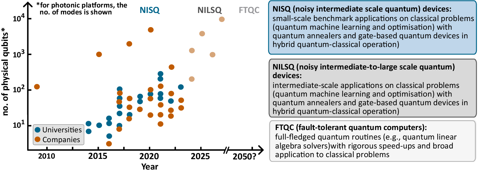
Figure 1. Evolution of the number of physical qubits of quantum computing and quantum simulation platforms by several companies and university research groups. The underlying data was collected from online sources and journal publications(D:Wave, 2023; IBM, 2023; PASQAL, 2023; rigetti, 2023; Google QAI, 2023; AQT, 2023; Quantinuum, 2023; Zhong et al., Reference Zhong, Wang, Deng, Chen, Peng, Luo, Qin, Wu, Ding, Hu, Hu, Yang, Zhang, Li, Li, Jiang, Gan, Yang, You, Wang, Li, Liu, Lu and Pan2020; Scholl et al., Reference Scholl, Schuler, Williams, Eberharter, Barredo, Schymik, Lienhard, Henry, Lang, Lahaye, Läuchli and Browaeys2021; Wu et al., Reference Wu, Bao, Cao, Chen, Chen, Chen, Chung, Deng, Du, Fan, Gong, Guo, Guo, Guo, Han, Hong, Huang, Huo, Li, Li, Li, Li, Liang, Lin, Lin, Qian, Qiao, Rong, Su, Sun, Wang, Wang, Wu, Xu, Yan, Yang, Yang, Ye, Yin, Ying, Yu, Zha, Zhang, Zhang, Zhang, Zhang, Zhao, Zhao, Zhou, Zhu, Lu, Peng, Zhu and Pan2021; Semeghini et al., Reference Semeghini, Levine, Keesling, Ebadi, Wang, Bluvstein, Verresen, Pichler, Kalinowski, Samajdar, Omran, Sachdev, Vishwanath, Greiner, Vuletić and Lukin2021; Joshi et al., Reference Joshi, Kranzl, Schuckert, Lovas, Maier, Blatt, Knap and Roos2022; Ebadi et al., Reference Ebadi, Keesling, Cain, Wang, Levine, Bluvstein, Semeghini, Omran, Liu, Samajdar, Luo, Nash, Gao, Barak, Farhi, Sachdev, Gemelke, Zhou, Choi, Pichler, Wang, Greiner, Vuletić and Lukin2022). The shaded data points for future years were collected from the companies’ roadmaps (D:Wave, 2023; PASQAL, 2023; IBM, 2023; IonQ, 2023).
Box 1. Fundamental equations of earth system models (ESMs)
ESMs describe the evolution of the Earth system with time, given external forcings such as solar radiation and anthropogenic influences. They consist of coupled models of, e.g., the atmosphere, ocean, and land, Figure 2. For example, the state of the atmosphere is described by the equation of state
 $$ p=\rho RT $$
with pressure
 $ p $
, density
$ p $
, density
 $ \rho $
, the gas constant
$ \rho $
, the gas constant
 $ R $
, and temperature
$ R $
, and temperature
 $ T $
. The barometric law describes the variation of pressure with altitude
$ T $
. The barometric law describes the variation of pressure with altitude
 $ z $
$ z $
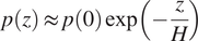 $$ p(z)\approx p(0)\exp \left(-\frac{z}{H}\right) $$
with the atmospheric scale height
 $ H $
.
$ H $
.
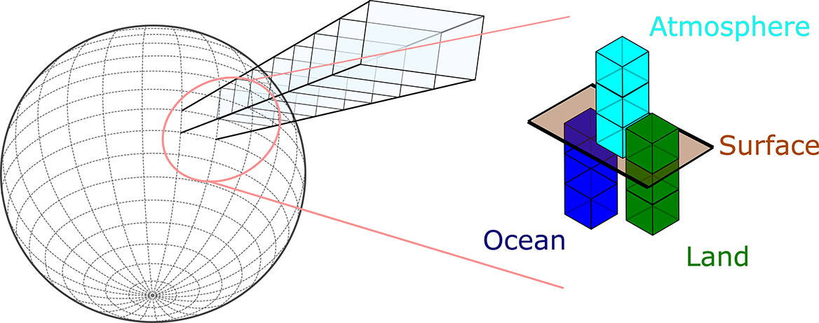
Figure 2. Schematic of an Earth system model (ESM). The ESM represents the state of the atmosphere, ocean and sea ice, and land using a grid covering the globe. For each component, physical properties such as water content in the atmosphere and soil or salinity of the ocean, the kinetic energy contained in the wind and currents, and the thermal energy contained in the temperature are represented. Following Gettelman and Rood (Reference Gettelman and Rood2016).
The dynamical properties of the atmosphere determine the evolution of mass, momentum, and energy. Mass conservation is expressed as the continuity equation
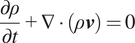 $$ \frac{\partial \rho }{\partial t}+\nabla \cdot \left(\rho \boldsymbol{v}\right)=0 $$
with the three-dimensional wind
 $ \boldsymbol{v} $
. The conservation of momentum in the system rotating with angular velocity
$ \boldsymbol{v} $
. The conservation of momentum in the system rotating with angular velocity
 $ \Omega $
is described by the Navier–Stokes equation
$ \Omega $
is described by the Navier–Stokes equation
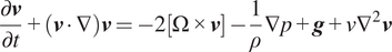 $$ \frac{\partial \boldsymbol{v}}{\partial t}+\left(\boldsymbol{v}\cdot \nabla \right)\boldsymbol{v}=-2\left[\Omega \times \boldsymbol{v}\right]-\frac{1}{\rho}\nabla p+\boldsymbol{g}+\nu {\nabla}^2\boldsymbol{v} $$
with apparent gravitational acceleration
 $ \boldsymbol{g} $
and kinematic viscosity
$ \boldsymbol{g} $
and kinematic viscosity
 $ \nu $
. Finally, the first law of thermodynamics results in the conservation of energy
$ \nu $
. Finally, the first law of thermodynamics results in the conservation of energy
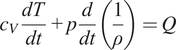 $$ {c}_V\frac{dT}{dt}+p\frac{d}{dt}\left(\frac{1}{\rho}\right)=Q $$
with the specific heat at constant volume
 $ {c}_V $
and the diabatic heating term
$ {c}_V $
and the diabatic heating term
 $ Q $
, which can be driven by absorption and emission of radiative energy or condensation and evaporation of water.
$ Q $
, which can be driven by absorption and emission of radiative energy or condensation and evaporation of water.
In this perspective, we discuss how we foresee leveraging the potential of quantum computing in the context of climate modeling. First, we give an introduction to data-driven, ML-based climate modeling and to quantum computing. Then, we discuss the potential of quantum computers for climate modeling, especially pointing out algorithms available for current noisy intermediate-scale quantum (NISQ) devices. Finally, we discuss the next steps towards developing a climate model improved with quantum computing.
2. Climate modeling
Climate models are three-dimensional models based on fundamental laws of physics (Jacobson, Reference Jacobson2005), see Box 1. The atmosphere is discretized over a horizontal grid covering the surface of the Earth, and vertical columns above each grid cell. In each grid box, state variables describe the physical properties, see Box 1. During a time step of the simulation, the evolution of energy and mass and the motions of air and tracers are solved. Earth system models (ESMs) simulate the interactive carbon and other biogeochemical cycles in addition to the atmosphere, land, ocean, and sea ice physical states (Eyring et al., Reference Eyring, Mishra, Griffith, Chen, Keenan, Turetsky, Brown, Jotzo, Moore and van der Linden2021b). Climate models and ESMs can simulate the mean state of the system, as well as natural variability, and how it may change given an external forcing (e.g., increasing the concentration of greenhouse gases). Not all relevant processes can be described by solving the fundamental equations, either because the resolution is not high enough (e.g., for shallow convection) or because the processes are not described by the equations (e.g., the formation of clouds and their influence on radiation transfer). Parameterizations represent the effects on the grid scale of the unresolved (subgrid-scale) processes as a function of the coarse-scale state variables. There have been many attempts to develop kilometre-resolution models that require fewer parameterizations and produce better input states for the remaining ones (Neumann et al., Reference Neumann, Düben, Adamidis, Bauer, Brück, Kornblueh, Klocke, Stevens, Wedi and Biercamp2019; Stevens et al., Reference Stevens, Satoh, Auger, Biercamp, Bretherton, Chen, Düben, Judt, Khairoutdinov, Klocke, Kodama, Kornblueh, Lin, Neumann, Putman, Röber, Shibuya, Vanniere, Vidale, Wedi and Zhou2019, Reference Stevens, Adami, Ali, Anzt, Aslan, Attinger, Bäck, Baehr, Bauer, Bernier, Bishop, Bockelmann, Bony, Brasseur, Bresch, Breyer, Brunet, Buttigieg, Cao, Castet, Cheng, Dey Choudhury, Coen, Crewell, Dabholkar, Dai, Doblas-Reyes, Durran, El Gaidi, Ewen, Exarchou, Eyring, Falkinhoff, Farrell, Forster, Frassoni, Frauen, Fuhrer, Gani, Gerber, Goldfarb, Grieger, Gruber, Hazeleger, Herken, Hewitt, Hoefler, Hsu, Jacob, Jahn, Jakob, Jung, Kadow, Kang, Kang, Kashinath, Kleinen-von Königslöw, Klocke, Kloenne, Klöwer, Kodama, Kollet, Kölling, Kontkanen, Kopp, Koran, Kulmala, Lappalainen, Latifi, Lawrence, Lee, Lejeun, Lessig, Li, Lippert, Luterbacher, Manninen, Marotzke, Matsouoka, Merchant, Messmer, Michel, Michielsen, Miyakawa, Müller, Munir, Narayanasetti, Ndiaye, Nobre, Oberg, Oki, Özkan Haller, Palmer, Posey, Prein, Primus, Pritchard, Pullen, Putrasahan, Quaas, Raghavan, Ramaswamy, Rapp, Rauser, Reichstein, Revi, Saluja, Satoh, Schemann, Schemm, Schnadt Poberaj, Schulthess, Senior, Shukla, Singh, Slingo, Sobel, Solman, Spitzer, Stier, Stocker, Strock, Su, Taalas, Taylor, Tegtmeier, Teutsch, Tompkins, Ulbrich, Vidale, Wu, Xu, Zaki, Zanna, Zhou and Ziemen2024), yet even these do not eliminate the need for running ensembles of climate models nor can they completely resolve all key processes (e.g., shallow clouds). Besides the large computational costs, storing the output of high-resolution models is problematic. Even today, the cost and bandwidth of storage systems do not keep up with the available computing power (Schär et al., Reference Schär, Fuhrer, Arteaga, Ban, Charpilloz, Girolamo, Hentgen, Hoefler, Lapillonne, Leutwyler, Osterried, Panosetti, Rüdisühli, Schlemmer, Schulthess, Sprenger, Ubbiali and Wernli2020). Especially the output of large ensembles of high-resolution climate models is impossible to store in its entirety, so that data needs to be coarse-grained or directly analysed while the simulations are running, and simulations need to be rerun when a specific analysis is required, trading storage for computation (Schär et al., Reference Schär, Fuhrer, Arteaga, Ban, Charpilloz, Girolamo, Hentgen, Hoefler, Lapillonne, Leutwyler, Osterried, Panosetti, Rüdisühli, Schlemmer, Schulthess, Sprenger, Ubbiali and Wernli2020). Therefore, to enable high-resolution ensemble runs, there is an urgent need to accelerate climate models.
Box 2. Qubits, quantum gates, and entanglement
The fundamental quantum information unit is the qubit. The state
 $ \mid \psi \Big\rangle $
of a qubit is a vector in a two-dimensional complex vector space, written as a superposition
$ \mid \psi \Big\rangle $
of a qubit is a vector in a two-dimensional complex vector space, written as a superposition
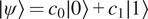 $ \mid \psi \left\rangle ={c}_0\mid 0\right\rangle +{c}_1\mid 1\Big\rangle $
of the two computational basis states
$ \mid \psi \left\rangle ={c}_0\mid 0\right\rangle +{c}_1\mid 1\Big\rangle $
of the two computational basis states
 $ \mid 0\Big\rangle $
and
$ \mid 0\Big\rangle $
and
 $ \mid 1\Big\rangle $
(Figure 3). Measuring the qubit in this basis yields
$ \mid 1\Big\rangle $
(Figure 3). Measuring the qubit in this basis yields
 $ 0 $
or
$ 0 $
or
 $ 1 $
with probability
$ 1 $
with probability
 $ {\left|{c}_0\right|}^2 $
or
$ {\left|{c}_0\right|}^2 $
or
 $ {\left|{c}_1\right|}^2 $
, respectively, with subsequent collapse of
$ {\left|{c}_1\right|}^2 $
, respectively, with subsequent collapse of
 $ \mid \psi \Big\rangle $
in the associated basis state. Qubits can be manipulated by means of quantum gates, which are unitary operators acting on the state vectors.
$ \mid \psi \Big\rangle $
in the associated basis state. Qubits can be manipulated by means of quantum gates, which are unitary operators acting on the state vectors.
The superposition principle extends to the case of many qubits. The state of
 $ N $
qubits has the form
$ N $
qubits has the form
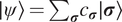 $ \mid \psi \left\rangle ={\sum}_{\boldsymbol{\sigma}}{c}_{\boldsymbol{\sigma}}\mid \boldsymbol{\sigma} \right\rangle $
, where
$ \mid \psi \left\rangle ={\sum}_{\boldsymbol{\sigma}}{c}_{\boldsymbol{\sigma}}\mid \boldsymbol{\sigma} \right\rangle $
, where
 $ \boldsymbol{\sigma} $
denotes one of the
$ \boldsymbol{\sigma} $
denotes one of the
 $ {2}^N $
possible bitstrings indexing the computational basis states, and
$ {2}^N $
possible bitstrings indexing the computational basis states, and
 $ {\left|{c}_{\sigma}\right|}^2 $
the probability of obtaining
$ {\left|{c}_{\sigma}\right|}^2 $
the probability of obtaining
 $ \boldsymbol{\sigma} $
as the outcome of a measurement in the same basis. An example of a two-qubit state has the form
$ \boldsymbol{\sigma} $
as the outcome of a measurement in the same basis. An example of a two-qubit state has the form
 $ \mid \psi \Big\rangle =\left(|01\Big\rangle +|10\Big\rangle \right)/\sqrt{2} $
. This is an example of an entangled state, where the qubits share non-local quantum correlations which result in correlated outcomes once they are measured (Nielsen and Chuang, Reference Nielsen and Chuang2010). Entanglement is generated using quantum gates that make selected qubits interact, and is a key ingredient for quantum computational advantage. The entanglement content of a quantum state is related to the computational complexity of representing it by classical means (Eisert et al., Reference Eisert, Cramer and Plenio2010), which generally requires computational resources scaling exponentially with the number of qubits
$ \mid \psi \Big\rangle =\left(|01\Big\rangle +|10\Big\rangle \right)/\sqrt{2} $
. This is an example of an entangled state, where the qubits share non-local quantum correlations which result in correlated outcomes once they are measured (Nielsen and Chuang, Reference Nielsen and Chuang2010). Entanglement is generated using quantum gates that make selected qubits interact, and is a key ingredient for quantum computational advantage. The entanglement content of a quantum state is related to the computational complexity of representing it by classical means (Eisert et al., Reference Eisert, Cramer and Plenio2010), which generally requires computational resources scaling exponentially with the number of qubits
 $ N $
. Classically intractable quantum states can be prepared on quantum computers, and their properties can be measured. This translates to the ability of preparing and sampling from otherwise intractable probability distributions
$ N $
. Classically intractable quantum states can be prepared on quantum computers, and their properties can be measured. This translates to the ability of preparing and sampling from otherwise intractable probability distributions
 $ {\left|{c}_{\boldsymbol{\sigma}}\right|}^2 $
, which can encode the solution to given problems.
$ {\left|{c}_{\boldsymbol{\sigma}}\right|}^2 $
, which can encode the solution to given problems.
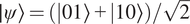
Figure 3. Representation of a qubit state as a vector on the Bloch sphere. The poles correspond to the basis states
 $ \mid 0\Big\rangle $
and
$ \mid 0\Big\rangle $
and
 $ \mid 1\Big\rangle $
.
$ \mid 1\Big\rangle $
.
Even high-resolution simulations require the use of some parameterizations, such as for microphysics and turbulence, and these still cause biases (Stevens et al., Reference Stevens, Satoh, Auger, Biercamp, Bretherton, Chen, Düben, Judt, Khairoutdinov, Klocke, Kodama, Kornblueh, Lin, Neumann, Putman, Röber, Shibuya, Vanniere, Vidale, Wedi and Zhou2019; Eyring et al., Reference Eyring, Gentine, Camps-Valls, Lawrence and Reichstein2024b). These, as well as the parameterizations used in coarser-scale climate models, could be improved with ML methods (Bracco et al., Reference Bracco, Brajard, Dijkstra, Hassanzadeh, Lessig and Monteleoni2025; Eyring et al., Reference Eyring, Gentine, Camps-Valls, Lawrence and Reichstein2024b) that learn from short high-resolution model simulations or observations to represent processes that are unresolved by coarse climate models. Challenges remain (Eyring et al., Reference Eyring, Collins, Gentine, Barnes, Barreiro, Beucler, Bocquet, Bretherton, Christensen, Dagon, Gagne, Hall, Hammerling, Hoyer, Iglesias-Suarez, Lopez-Gomez, McGraw, Meehl, Molina, Monteleoni, Mueller, Pritchard, Rolnick, Runge, Stier, Watt-Meyer, Weigel, Yu and Zanna2024a) among which: 1) instabilities when ML-based parameterizations are coupled to the climate model, often due to the models learning spurious causal relationships (Brenowitz et al., Reference Brenowitz, Beucler, Pritchard and Bretherton2020); 2) difficulty in generalizing beyond the training regime (Rasp et al., Reference Rasp, Pritchard and Gentine2018), which is highly relevant in a changing climate, where the mean and extremes of climate variable distributions are shifting (Gentine et al., Reference Gentine, Eyring, Beucler, Camps-Valls, Tuia, Zhu and Reichstein2021). These challenges demonstrate the need for more expressive models (i.e., models that can learn a large variety of functions) that can be trained efficiently using potentially limited datasets.
All classical parameterizations as well as some data-driven ones (Grundner et al., Reference Grundner, Beucler, Gentine and Eyring2024; Pahlavan et al., Reference Pahlavan, Hassanzadeh and Alexander2024), have parameters that need to be estimated to reduce the mismatch between observations and model results (Hourdin et al., Reference Hourdin, Mauritsen, Gettelman, Golaz, Balaji, Duan, Folini, Ji, Klocke, Qian, Rauser, Rio, Tomassini, Watanabe and Williamson2017). This tuning is a very time-consuming process requiring considerable expert knowledge and computing time, which motivates the development of automatic algorithms to improve its efficiency and reproducibility (Hourdin et al., Reference Hourdin, Mauritsen, Gettelman, Golaz, Balaji, Duan, Folini, Ji, Klocke, Qian, Rauser, Rio, Tomassini, Watanabe and Williamson2017; Bonnet et al., Reference Bonnet, Pastori, Schwabe, Giorgetta, Iglesias-Suarez and Eyring2024). The tuned model should be evaluated against other climate models and against observations, in which novel techniques can be used to classify data sets and develop better-suited products (Kaps et al., Reference Kaps, Lauer, Camps-Valls, Gentine, Gomez-Chova and Eyring2023).
Summing up, there is an urgent need for faster and better climate models capable of running at high resolution, for more accurate and generalizable parameterizations, and for fast, reliable tuning and evaluation methods, also beyond classical ML algorithms.
3. Quantum computing: current status and challenges
The field of quantum computation deals with developing and controlling quantum systems to store and process information in ways that go beyond the capabilities of standard (classical) computers (Nielsen and Chuang, Reference Nielsen and Chuang2010), see Box 2. Quantum computers hold the promise of efficiently executing tasks intractable even for the largest supercomputer, including simulations of complex materials and chemicals, and solving optimization problems (Grumbling and Horowitz, Reference Grumbling and Horowitz2019). Despite extraordinary theoretical and experimental developments in the last decades, we are still in the era of NISQ devices—– noisy intermediate-scale quantum devices counting up to few hundreds qubits, with several limitations caused by noise (Preskill, Reference Preskill2018). Despite these limitations, NISQ devices can already be used to tackle problems of academic interest, and it is foreseeable that quantum error correction methods will bring us fault-tolerant quantum computers in the future (Devitt et al., Reference Devitt, Munro and Nemoto2013; Campbell et al., Reference Campbell, Terhal and Vuillot2017), see Figure 1. It is thus important to ask now whether the algorithms developed for quantum computers could help address the challenges faced by climate modelling (Singh et al., Reference Singh, Dhara, Kumar, Gill and Uhlig2022; Nivelkar et al., Reference Nivelkar, Bhirud, Singh, Ranjan and Kumar2023; Otgonbaatar et al., Reference Otgonbaatar, Nurmi, Johansson, Mäkelä, Kocman, Gawron, Puchała, Mielzcarek, Miroszewski and Dumitru2023; Rahman et al., Reference Rahman, Alkhalaf, Alam, Tiwari, Shafiullah, Al-Judaibi and Al-Ismail2024; Bazgir and Zhang, Reference Bazgir and Zhang2024). In the following, we review several relevant quantum computing paradigms and algorithms.
3.1. Quantum linear algebra solvers
Quantum linear algebra solvers make use of the fact that quantum computation using
 $ N $
qubits is mathematically described by linear operators in vector spaces of (large) dimension
$ N $
qubits is mathematically described by linear operators in vector spaces of (large) dimension
 $ {2}^N $
. Linear problems of size
$ {2}^N $
. Linear problems of size
 $ M $
can be encoded in quantum states and operators using only logarithmically many qubits (in
$ M $
can be encoded in quantum states and operators using only logarithmically many qubits (in
 $ M $
). Provided this encoding, quantum solvers offer exponential improvements in terms of resources needed to solve a problem, requiring only
$ M $
). Provided this encoding, quantum solvers offer exponential improvements in terms of resources needed to solve a problem, requiring only
 $ \mathcal{O}\left(\mathrm{poly}\log M\right) $
qubits and gates compared to the
$ \mathcal{O}\left(\mathrm{poly}\log M\right) $
qubits and gates compared to the
 $ \mathcal{O}\left(\mathrm{poly}M\right) $
operations required for classical algorithms (Harrow et al., Reference Harrow, Hassidim and Lloyd2009). They can therefore significantly speed up large matrix operations, e.g., in the resolution of (partial) differential equations using finite difference/elements methods (Berry, Reference Berry2014; Lloyd et al., Reference Lloyd, Palma, Gokler, Kiani, Liu, Marvian, Tennie and Palmer2020; Li et al., Reference Li, Yin, Wiebe, Chun, Schenter, Cheung and Mülmenstädt2023). This exponential speedup depends on the ability of efficiently (i.e., with costs scaling polynomially in the number of qubits) encoding the problem data in the states and operators on the quantum device, and on the efficient readout of the properties of interest from the quantum state encoding the solution. These challenges, together with the limitations due to noise, restrict the current applicability of these routines to small-scale problems (Cai et al., Reference Cai, Weedbrook, Su, Chen, Gu, Zhu, Li, Liu, Lu and Pan2013; Barz et al., Reference Barz, Kassal, Ringbauer, Lipp, Dakić, Aspuru-Guzik and Walther2014; Zheng et al., Reference Zheng, Song, Chen, Xia, Liu, Guo, Zhang, Xu, Deng, Huang, Wu, Yan, Zheng, Lu, Pan, Wang, Lu and Zhu2017).
$ \mathcal{O}\left(\mathrm{poly}M\right) $
operations required for classical algorithms (Harrow et al., Reference Harrow, Hassidim and Lloyd2009). They can therefore significantly speed up large matrix operations, e.g., in the resolution of (partial) differential equations using finite difference/elements methods (Berry, Reference Berry2014; Lloyd et al., Reference Lloyd, Palma, Gokler, Kiani, Liu, Marvian, Tennie and Palmer2020; Li et al., Reference Li, Yin, Wiebe, Chun, Schenter, Cheung and Mülmenstädt2023). This exponential speedup depends on the ability of efficiently (i.e., with costs scaling polynomially in the number of qubits) encoding the problem data in the states and operators on the quantum device, and on the efficient readout of the properties of interest from the quantum state encoding the solution. These challenges, together with the limitations due to noise, restrict the current applicability of these routines to small-scale problems (Cai et al., Reference Cai, Weedbrook, Su, Chen, Gu, Zhu, Li, Liu, Lu and Pan2013; Barz et al., Reference Barz, Kassal, Ringbauer, Lipp, Dakić, Aspuru-Guzik and Walther2014; Zheng et al., Reference Zheng, Song, Chen, Xia, Liu, Guo, Zhang, Xu, Deng, Huang, Wu, Yan, Zheng, Lu, Pan, Wang, Lu and Zhu2017).
3.2. Quantum annealing for optimization problems
Quantum annealing offers a way of solving optimization problems on quantum devices (Das and Chakrabarti, Reference Das and Chakrabarti2008; Albash and Lidar, Reference Albash and Lidar2018). Quantum annealers address combinatorial problems with a discrete solution space. The solution to a given problem is encoded in the ground state of an Ising Hamiltonian (Das and Chakrabarti, Reference Das and Chakrabarti2008). This Hamiltonian is then realized on a quantum device, the annealer, and its ground state prepared by slowly steering an initial state towards it. In this way, the implemented quantum state globally explores the optimization landscape before tunnelling towards the optimal solution. Quantum annealers consisting of thousands of qubits are already available for use in academic and industrial applications (Yarkoni et al., Reference Yarkoni, Raponi, Bäck and Schmitt2022). This approach is potentially scalable to large problems, and the first claims of quantum advantage with quantum annealers have been made (King et al., Reference King, Nocera, Rams, Dziarmaga, Wiersema, Bernoudy, Raymond, Kaushal, Heinsdorf, Harris, Boothby, Altomare, Berkley, Boschnak, Chern, Christiani, Cibere, Connor, Dehn, Deshpande, Ejtemaee, Farré, Hamer, Hoskinson, Huang, Johnson, Kortas, Ladizinsky, Lai, Lanting, Li, MacDonald, Marsden, McGeoch, Molavi, Neufeld, Norouzpour, Oh, Pasvolsky, Poitras, Poulin-Lamarre, Prescott, Reis, Rich, Samani, Sheldan, Smirnov, Sterpka, Clavera, Tsai, Volkmann, Whiticar, Whittaker, Wilkinson, Yao, Yi, Sandvik, Alvarez, Melko, Carrasquilla, Franz and Amin2024). However, noise is an open problem for quantum annealers (also due to the lack of fully fault-tolerant quantum annealing schemes (Pudenz et al., Reference Pudenz, Albash and Lidar2014)).
3.3. Parameterized quantum circuit models
Parameterized quantum circuits (PQCs) are sequences of quantum gates depending on tunable parameters
 $ \boldsymbol{\theta} $
that are optimized for the quantum device to solve a given problem. Applications include variational quantum eigensolvers (Peruzzo et al., Reference Peruzzo, McClean, Shadbolt, Yung, Zhou, Love, Aspuru-Guzik and O’Brien2014), quantum approximate optimization algorithms (Farhi et al., Reference Farhi, Goldstone and Gutmann2014), and quantum machine learning (QML) (Schuld and Petruccione, Reference Schuld and Petruccione2018; Schuld et al., Reference Schuld, Sinayskiy and Petruccione2015; Biamonte et al., Reference Biamonte, Wittek, Pancotti, Rebentrost, Wiebe and Lloyd2017; Dunjko and Briegel, Reference Dunjko and Briegel2018; Schuld and Petruccione, Reference Schuld and Petruccione2018; Cerezo et al., Reference Cerezo, Verdon, Huang, Cincio and Coles2022). PQCs are NISQ-friendly due to their limited depth, supplemented by the optimization of the parameters
$ \boldsymbol{\theta} $
that are optimized for the quantum device to solve a given problem. Applications include variational quantum eigensolvers (Peruzzo et al., Reference Peruzzo, McClean, Shadbolt, Yung, Zhou, Love, Aspuru-Guzik and O’Brien2014), quantum approximate optimization algorithms (Farhi et al., Reference Farhi, Goldstone and Gutmann2014), and quantum machine learning (QML) (Schuld and Petruccione, Reference Schuld and Petruccione2018; Schuld et al., Reference Schuld, Sinayskiy and Petruccione2015; Biamonte et al., Reference Biamonte, Wittek, Pancotti, Rebentrost, Wiebe and Lloyd2017; Dunjko and Briegel, Reference Dunjko and Briegel2018; Schuld and Petruccione, Reference Schuld and Petruccione2018; Cerezo et al., Reference Cerezo, Verdon, Huang, Cincio and Coles2022). PQCs are NISQ-friendly due to their limited depth, supplemented by the optimization of the parameters
 $ \boldsymbol{\theta} $
that is achieved iteratively in a hybrid quantum-classical manner (Cerezo et al., Reference Cerezo, Arrasmith, Babbush, Benjamin, Endo, Fujii, McClean, Mitarai, Yuan, Cincio and Coles2021; Bharti et al., Reference Bharti, Cervera-Lierta, Kyaw, Haug, Alperin-Lea, Anand, Degroote, Heimonen, Kottmann, Menke, Mok, Sim, Kwek and Aspuru-Guzik2022): a cost function is measured on the quantum device and fed to a classical routine that proposes new
$ \boldsymbol{\theta} $
that is achieved iteratively in a hybrid quantum-classical manner (Cerezo et al., Reference Cerezo, Arrasmith, Babbush, Benjamin, Endo, Fujii, McClean, Mitarai, Yuan, Cincio and Coles2021; Bharti et al., Reference Bharti, Cervera-Lierta, Kyaw, Haug, Alperin-Lea, Anand, Degroote, Heimonen, Kottmann, Menke, Mok, Sim, Kwek and Aspuru-Guzik2022): a cost function is measured on the quantum device and fed to a classical routine that proposes new
 $ \boldsymbol{\theta} $
for the next iteration. This results in shorter and classically optimized circuits that can run within the coherence time of NISQ devices.
$ \boldsymbol{\theta} $
for the next iteration. This results in shorter and classically optimized circuits that can run within the coherence time of NISQ devices.
In the context of QML, PQCs find applications in regression, classification, and generative modeling tasks (Cerezo et al., Reference Cerezo, Verdon, Huang, Cincio and Coles2022). In regression and classification, PQCs are used as function approximators and are often referred to as quantum neural networks (QNNs) (Farhi and Neven, Reference Farhi and Neven2018). Classical input data
 $ \boldsymbol{x} $
first is encoded in a quantum state
$ \boldsymbol{x} $
first is encoded in a quantum state
 $ \mid \phi \left(\boldsymbol{x}\right)\Big\rangle $
. Then the output is calculated as the expectation value of an observable in the output state
$ \mid \phi \left(\boldsymbol{x}\right)\Big\rangle $
. Then the output is calculated as the expectation value of an observable in the output state
 $ \mid \psi \left(\boldsymbol{x};\boldsymbol{\theta} \right)\left\rangle ={\hat{U}}_{\boldsymbol{\theta}}\mid \phi \left(\boldsymbol{x}\right)\right\rangle $
, where
$ \mid \psi \left(\boldsymbol{x};\boldsymbol{\theta} \right)\left\rangle ={\hat{U}}_{\boldsymbol{\theta}}\mid \phi \left(\boldsymbol{x}\right)\right\rangle $
, where
 $ {\hat{U}}_{\boldsymbol{\theta}} $
denotes the action of the PQC. The embedding
$ {\hat{U}}_{\boldsymbol{\theta}} $
denotes the action of the PQC. The embedding
 $ \boldsymbol{x}\to \mid \phi \left(\boldsymbol{x}\right)\Big\rangle $
needs to be carefully chosen as it strongly influences the model performance (Schuld and Petruccione, Reference Schuld and Petruccione2018; Pérez-Salinas et al., Reference Pérez-Salinas, Cervera-Lierta, Gil-Fuster and Latorre2020; Schuld et al., Reference Schuld, Sweke and Meyer2021), and potentially requires compression strategies (Dilip et al., Reference Dilip, Liu, Smith and Pollmann2022). The higher expressivity of QNNs (Du et al., Reference Du, Hsieh, Liu and Tao2020, Reference Du, Hsieh, Liu, You and Tao2021; Yu et al., Reference Yu, Chen, Jiao, Li, Lu, Wang and Yang2023b), makes them interesting ansatzes for ML tasks. Furthermore, several works have investigated their generalization properties, with promising results (Cong et al., Reference Cong, Choi and Lukin2019; Abbas et al., Reference Abbas, Sutter, Zoufal, Lucchi, Figalli and Woerner2021; Caro et al., Reference Caro, Huang, Cerezo, Sharma, Sornborger, Cincio and Coles2022, Reference Caro, Huang, Ezzell, Gibbs, Sornborger, Cincio, Coles and Holmes2023). Regarding their trainability, while suitably designed QNNs show desirable geometrical properties that may lead to faster training (Abbas et al., Reference Abbas, Sutter, Zoufal, Lucchi, Figalli and Woerner2021), in general, the training of PQCs can be hindered by the presence of barren plateaus (Ragone et al., Reference Ragone, Bakalov, Sauvage, Kemper, Marrero, Larocca and Cerezo2024) and potentially requires advanced initialization strategies (Zhang et al., Reference Zhang, Liu, Hsieh, Tao, Koyejo, Mohamed, Agarwal, Belgrave, Cho and Oh2022). However, in quantum convolutional neural networks (QCNNs), barren plateaus do not seem to be a problem (Pesah et al., Reference Pesah, Cerezo, Wang, Volkoff, Sornborger and Coles2021).
$ \boldsymbol{x}\to \mid \phi \left(\boldsymbol{x}\right)\Big\rangle $
needs to be carefully chosen as it strongly influences the model performance (Schuld and Petruccione, Reference Schuld and Petruccione2018; Pérez-Salinas et al., Reference Pérez-Salinas, Cervera-Lierta, Gil-Fuster and Latorre2020; Schuld et al., Reference Schuld, Sweke and Meyer2021), and potentially requires compression strategies (Dilip et al., Reference Dilip, Liu, Smith and Pollmann2022). The higher expressivity of QNNs (Du et al., Reference Du, Hsieh, Liu and Tao2020, Reference Du, Hsieh, Liu, You and Tao2021; Yu et al., Reference Yu, Chen, Jiao, Li, Lu, Wang and Yang2023b), makes them interesting ansatzes for ML tasks. Furthermore, several works have investigated their generalization properties, with promising results (Cong et al., Reference Cong, Choi and Lukin2019; Abbas et al., Reference Abbas, Sutter, Zoufal, Lucchi, Figalli and Woerner2021; Caro et al., Reference Caro, Huang, Cerezo, Sharma, Sornborger, Cincio and Coles2022, Reference Caro, Huang, Ezzell, Gibbs, Sornborger, Cincio, Coles and Holmes2023). Regarding their trainability, while suitably designed QNNs show desirable geometrical properties that may lead to faster training (Abbas et al., Reference Abbas, Sutter, Zoufal, Lucchi, Figalli and Woerner2021), in general, the training of PQCs can be hindered by the presence of barren plateaus (Ragone et al., Reference Ragone, Bakalov, Sauvage, Kemper, Marrero, Larocca and Cerezo2024) and potentially requires advanced initialization strategies (Zhang et al., Reference Zhang, Liu, Hsieh, Tao, Koyejo, Mohamed, Agarwal, Belgrave, Cho and Oh2022). However, in quantum convolutional neural networks (QCNNs), barren plateaus do not seem to be a problem (Pesah et al., Reference Pesah, Cerezo, Wang, Volkoff, Sornborger and Coles2021).
The embedding
 $ \boldsymbol{x}\to \mid \phi \left(\boldsymbol{x}\right)\Big\rangle $
can be thought of as a feature map from the input
$ \boldsymbol{x}\to \mid \phi \left(\boldsymbol{x}\right)\Big\rangle $
can be thought of as a feature map from the input
 $ \boldsymbol{x} $
to the (large) Hilbert space of quantum states (Schuld and Killoran, Reference Schuld and Killoran2019; Havlíček et al., Reference Havlíček, Córcoles, Temme, Harrow, Kandala, Chow and Gambetta2019). This observation constitutes the basis of quantum kernel methods (Schuld and Killoran, Reference Schuld and Killoran2019; Havlíček et al., Reference Havlíček, Córcoles, Temme, Harrow, Kandala, Chow and Gambetta2019), where quantum kernels are constructed from inner products
$ \boldsymbol{x} $
to the (large) Hilbert space of quantum states (Schuld and Killoran, Reference Schuld and Killoran2019; Havlíček et al., Reference Havlíček, Córcoles, Temme, Harrow, Kandala, Chow and Gambetta2019). This observation constitutes the basis of quantum kernel methods (Schuld and Killoran, Reference Schuld and Killoran2019; Havlíček et al., Reference Havlíček, Córcoles, Temme, Harrow, Kandala, Chow and Gambetta2019), where quantum kernels are constructed from inner products
 $ \left\langle \phi \left(\boldsymbol{x}\right)|\phi \left({\boldsymbol{x}}^{\prime}\right)\right\rangle $
measured on the quantum device. The constructed kernels are then used in subsequent tasks, e.g., in data classification (Havlíček et al., Reference Havlíček, Córcoles, Temme, Harrow, Kandala, Chow and Gambetta2019), or Gaussian process regression (Otten et al., Reference Otten, Goumiri, Priest, Chapline and Schneider2020; Rapp and Roth, Reference Rapp and Roth2024). Despite their advantage on specific datasets (Huang et al., Reference Huang, Broughton, Mohseni, Babbush, Boixo, Neven and McClean2021), quantum kernel methods may also suffer from trainability issues analogous to barren plateaus in QNNs (Thanasilp et al., Reference Thanasilp, Wang, Cerezo and Holmes2022), which highlights the requirement of a careful design.
$ \left\langle \phi \left(\boldsymbol{x}\right)|\phi \left({\boldsymbol{x}}^{\prime}\right)\right\rangle $
measured on the quantum device. The constructed kernels are then used in subsequent tasks, e.g., in data classification (Havlíček et al., Reference Havlíček, Córcoles, Temme, Harrow, Kandala, Chow and Gambetta2019), or Gaussian process regression (Otten et al., Reference Otten, Goumiri, Priest, Chapline and Schneider2020; Rapp and Roth, Reference Rapp and Roth2024). Despite their advantage on specific datasets (Huang et al., Reference Huang, Broughton, Mohseni, Babbush, Boixo, Neven and McClean2021), quantum kernel methods may also suffer from trainability issues analogous to barren plateaus in QNNs (Thanasilp et al., Reference Thanasilp, Wang, Cerezo and Holmes2022), which highlights the requirement of a careful design.
PQCs also find a natural application as generative models (Amin et al., Reference Amin, Andriyash, Rolfe, Kulchytskyy and Melko2018; Dallaire-Demers and Killoran, Reference Dallaire-Demers and Killoran2018; Coyle et al., Reference Coyle, Mills, Danos and Kashefi2020). The output state of a PQC indeed corresponds to a probability distribution over an exponentially large computational basis, via the relation
 $ {P}_{\boldsymbol{\theta}}\left(\boldsymbol{\sigma} \right)=\mid \Big\langle \boldsymbol{\sigma} \mid {\hat{U}}_{\boldsymbol{\theta}}{\left|{\phi}_0\Big\rangle \right|}^2 $
, with
$ {P}_{\boldsymbol{\theta}}\left(\boldsymbol{\sigma} \right)=\mid \Big\langle \boldsymbol{\sigma} \mid {\hat{U}}_{\boldsymbol{\theta}}{\left|{\phi}_0\Big\rangle \right|}^2 $
, with
 $ \boldsymbol{\sigma} $
indexing the computational basis states, and
$ \boldsymbol{\sigma} $
indexing the computational basis states, and
 $ \mid {\phi}_0\Big\rangle $
a predefined reference state. For generative tasks, the parameters
$ \mid {\phi}_0\Big\rangle $
a predefined reference state. For generative tasks, the parameters
 $ \boldsymbol{\theta} $
are optimized for
$ \boldsymbol{\theta} $
are optimized for
 $ {P}_{\boldsymbol{\theta}} $
to approximate the probability distribution underlying a set of training data. The PQC is then used to sample the distribution
$ {P}_{\boldsymbol{\theta}} $
to approximate the probability distribution underlying a set of training data. The PQC is then used to sample the distribution
 $ {P}_{\boldsymbol{\theta}} $
. These models have improved representational power over standard generative models (Du et al., Reference Du, Hsieh, Liu and Tao2020), but also require careful design to avoid trainability issues (Rudolph et al., Reference Rudolph, Lerch, Thanasilp, Kiss, Vallecorsa, Grossi and Holmes2023).
$ {P}_{\boldsymbol{\theta}} $
. These models have improved representational power over standard generative models (Du et al., Reference Du, Hsieh, Liu and Tao2020), but also require careful design to avoid trainability issues (Rudolph et al., Reference Rudolph, Lerch, Thanasilp, Kiss, Vallecorsa, Grossi and Holmes2023).
We finally remark that despite the several hints to potential advantages on specific tasks, it is not yet clear whether a practical advantage of QML on real-world classical datasets can be demonstrated. Among the practical hurdles are the aforementioned trainability issues, as well as the necessity of efficient coupling with HPC and the inevitable presence of noise.
3.4. Integrated high-performance quantum computing
PQCs are based on the interplay between a quantum and a classical component within a hybrid algorithm. NISQ systems thus need to be integrated with classical computing resources at the hardware level. As quantum circuits become more complex, the classical component in PQCs and thus the required computing resources will grow as well, to the scale of an HPC problem. Given the trend towards heterogeneous development of modern HPC systems, e.g., increasingly using hardware accelerators like graphics processing units (Schulz et al., Reference Schulz, Kranzlmüller, Schulz, Trinitis and Weidendorfer2021), this leads to consider quantum hardware as a new class of accelerators for dedicated tasks within HPC workflows (Humble et al., Reference Humble, McCaskey, Lyakh, Gowrishankar, Frisch and Monz2021; Rüfenacht et al., Reference Rüfenacht, Taketani, Lähteenmäki, Bergholm, Kranzlmüller, Schulz and Schulz2022). The high performance computing—quantum computing (HPCQC) integration is an interdisciplinary challenge with aspects at the hardware, software, programming, and algorithmic level. The hardware integration is crucial to reduce latencies, especially in iterative variational algorithms (Rüfenacht et al., Reference Rüfenacht, Taketani, Lähteenmäki, Bergholm, Kranzlmüller, Schulz and Schulz2022). Moreover, the development of a single software stack for integrated systems, including the offloading of tasks to quantum accelerators and the scheduling of those resources, is necessary for ensuring operation and a smooth user experience (Schulz et al., Reference Schulz, Ruefenacht, Kranzlmuller and Schulz2022).
The HPCQC integration is not a concept limited to the NISQ development phase of quantum hardware, but is also relevant for future, fault-tolerant systems. At that point, we expect that the HPC computational resources will have to take over further tasks related to the operation of the quantum hardware, like circuit compilation and error control (Davenport et al., Reference Davenport, Jones and Thomason2023; Maronese et al., Reference Maronese, Moro, Rocutto and Prati2022).
3.5. Error correction and mitigation
Current NISQ devices are still modest in qubit counts (tens to hundreds), circuit depths (accommodating up to a thousand gate operations), and coherence times (from microseconds to seconds, depending on the platform (Byrd and Ding, Reference Byrd and Ding2023)). The achievable circuit depth and the repetition rate influence the complexity and the practical applicability of QML models, respectively. Hardware noise may negatively impact QML trainability and is also one of the main limiting factors for quantum annealing and for fault-tolerant applications.
Achieving fault-tolerance is the goal of quantum error correction methods, in which one logical qubit is represented using several physical ones, to detect and correct errors at runtime (Devitt et al., Reference Devitt, Munro and Nemoto2013). This is a crucial requirement for quantum algorithms relying on extensive numbers of quantum operations, such as quantum linear algebra subroutines. Given the substantial resource overhead needed for quantum error correction (Davenport et al., Reference Davenport, Jones and Thomason2023), its practical implementation can be considered in its infancy despite recent rapid advances (Google Quantum AI and Collaborators, 2025).
Other techniques to reduce noise-induced biases, without correcting for faulty qubits or operations, go under the name of error mitigation and are based on post-processing measurements collected from a suitably defined ensemble of quantum computation runs (Cai et al., Reference Cai, Babbush, Benjamin, Endo, Huggins, Li, McClean and O’Brien2023). Many mitigation techniques are currently being researched, such as zero-noise extrapolation and probabilistic error cancellation (Cai et al., Reference Cai, Babbush, Benjamin, Endo, Huggins, Li, McClean and O’Brien2023). These are particularly relevant for NISQ-targeted applications, as they can be implemented with little overhead in the number of gates and qubits. Hence, they are promising for “de-noising” the predictions from PQC-based methods.
4. Quantum computing for climate modeling
We now move on to considering the potential that the quantum algorithms presented in the previous sections can have for climate modelling. We discuss potential applications in solving the underlying differential equations, in model tuning, analysis, and evaluation, and in improving subgrid-scale parameterizations (Figure 4).
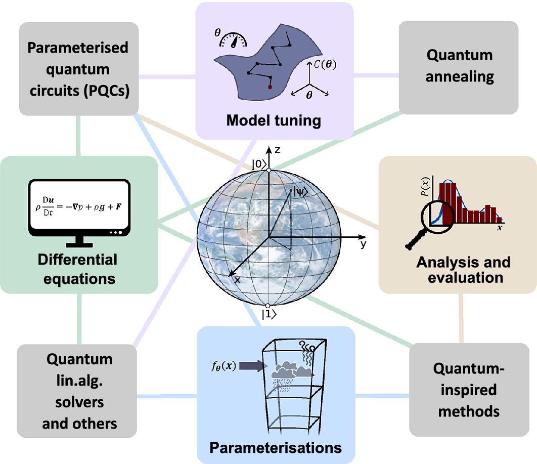
Figure 4. Overview of the climate modeling tasks and the category of matching quantum computing algorithms. (Image of the Earth by NASA/Apollo 17).
4.1. Accelerating the resolution of high-dimensional differential equations
Solving differential equations is at the root of climate modelling, especially in the atmosphere and ocean components. Dynamical conservation laws are represented by PDEs, and chemical reactions are described by ordinary differential equations (ODEs) (Alvanos and Christoudias, Reference Alvanos and Christoudias2019; Sander et al., Reference Sander, Kerkweg, Jöckel and Lelieveld2005; Zlatev et al., Reference Zlatev, Dimov, Faragó, Georgiev, Havasi, Lirkov and Margenov2022). The resources needed for solving them grow rapidly with increasing resolution of the models. This calls for methods for efficiently encoding and processing the climate state variables in all the model cells. Several quantum algorithms seeking an exponential reduction of the needed resources have been recently proposed in the context of computational fluid dynamics (Gaitan, Reference Gaitan2020; Steijl and Barakos, Reference Steijl and Barakos2018).
Methods for time-dependent fluid-flow problems have been developed in the framework of gate-based quantum computing (Steijl and Barakos, Reference Steijl and Barakos2018; Mezzacapo et al., Reference Mezzacapo, Sanz, Lamata, Egusquiza, Succi and Solano2015; Gaitan, Reference Gaitan2020) and quantum annealers (Ray et al., Reference Ray, Banerjee, Nadiga and Karra2019). For example, using spatial discretization of the PDEs, Gaitan (Reference Gaitan2020) reduces the one-dimensional Navier–Stokes equations to a system of ODEs
 $$ \frac{d\boldsymbol{U}}{dt}=f\left(\boldsymbol{U}\right), $$
with
 $ \boldsymbol{U} $
being a vector depending on
$ \boldsymbol{U} $
being a vector depending on
 $ \rho $
,
$ \rho $
,
 $ v $
, and
$ v $
, and
 $ T $
, and the driver function
$ T $
, and the driver function
 $ f\left(\boldsymbol{U}\right) $
depending on the discretization procedure. Kacewicz (Reference Kacewicz2006) showed that an almost optimal quantum algorithm exists for finding an approximate solution to a set of nonlinear ODEs. As shown by Gaitan (Reference Gaitan2020), the solution of Eq. (6) is approximated by discretizing it in both the spatial and time domains, and then determining the approximate solution using quantum amplitude estimation (QAEA) (Brassard et al., Reference Brassard, Høyer, Mosca, Tapp, Lomonaco and Brandt2002). These hybrid approaches for Navier–Stokes equations (Gaitan, Reference Gaitan2020) could thus potentially achieve up to exponential speed-up compared to deterministic classical algorithms, due to the quantum subroutine (Brassard et al., Reference Brassard, Høyer, Mosca, Tapp, Lomonaco and Brandt2002). However, the stability of such algorithms with respect to the spatial discretization still remains an open issue, and these methods inherit the challenges that quantum linear solvers may face, related to the data encoding and readout, and to the implementation of the linear operator defining the problem (Aaronson, Reference Aaronson2015).
$ f\left(\boldsymbol{U}\right) $
depending on the discretization procedure. Kacewicz (Reference Kacewicz2006) showed that an almost optimal quantum algorithm exists for finding an approximate solution to a set of nonlinear ODEs. As shown by Gaitan (Reference Gaitan2020), the solution of Eq. (6) is approximated by discretizing it in both the spatial and time domains, and then determining the approximate solution using quantum amplitude estimation (QAEA) (Brassard et al., Reference Brassard, Høyer, Mosca, Tapp, Lomonaco and Brandt2002). These hybrid approaches for Navier–Stokes equations (Gaitan, Reference Gaitan2020) could thus potentially achieve up to exponential speed-up compared to deterministic classical algorithms, due to the quantum subroutine (Brassard et al., Reference Brassard, Høyer, Mosca, Tapp, Lomonaco and Brandt2002). However, the stability of such algorithms with respect to the spatial discretization still remains an open issue, and these methods inherit the challenges that quantum linear solvers may face, related to the data encoding and readout, and to the implementation of the linear operator defining the problem (Aaronson, Reference Aaronson2015).
Quantum lattice–Boltzmann methods (QLBM) offer alternatives to quantum linear solvers, circumventing solving linear systems directly (Budinski, Reference Budinski2021, Reference Budinski2022; Schalkers and Möller, Reference Schalkers and Möller2022). The lattice–Boltzmann method, a mesoscopic stream-and-collide method for probability densities of fluid particles, lends itself to quantum solution natively and efficiently (Budinski et al., Reference Budinski, Niemimäki, Zamora-Zamora and Lahtinen2023; Li et al., Reference Li, Yin, Wiebe, Chun, Schenter, Cheung and Mülmenstädt2023). QLBM algorithms can be fully quantum (Budinski, Reference Budinski2021), or hybrid, such as Budinski’s Navier–Stokes algorithm (Budinski, Reference Budinski2022), where quantum-classical communication is needed to incorporate non-linearities. Other approaches for non-linearities in QLBM exist, e.g., by using Carleman linearization (Itani and Succi, Reference Itani and Succi2022). Koopman operators can also be used to induce linearity (Bondar et al., Reference Bondar, Gay-Balmaz and Tronci2019). Also, QLBM faces the challenge related to data readout and encoding: for some QLBM models, this must be repeated at all time steps, which makes efficient time-marching a problem of prime importance for QLBM.
Data-driven quantum-assisted approaches are also a possibility to predict the evolution of climate systems, as demonstrated by Jaderberg et al. (Reference Jaderberg, Gentile, Ghosh, Elfving, Jones, Vodola, Manobianco and Weiss2024) in the context of weather models.
In summary, the encoding and readout of classical variables is one of the primary limitations that need to be addressed for applying the aforementioned routines to problems on scales of a climate model. Even though 30 logical qubits could be sufficient to store one billion climate variables (Tennie and Palmer, Reference Tennie and Palmer2023) and to implement their time evolution using quantum circuits of polynomial depth, it is still unclear what type of climate states can be efficiently encoded in quantum states, and which properties of the climate can be efficiently measured. Although full quantum state reconstruction is not experimentally feasible for large quantum systems (it requires a number of measurements growing exponentially in the number of qubits (Struchalin et al., Reference Struchalin, Zagorovskii, Kovlakov, Straupe and Kulik2021)), fundamental insights on the properties that can be efficiently read out from quantum states exist in the framework of shadow tomography (Huang et al., Reference Huang, Kueng and Preskill2020): these results will need to be adapted to the specific use-case of climate simulation and subsequent evaluation.
4.2. QML-based parameterizations
QML models, such as QNNs, can be used to develop data-driven parameterizations by training them with data from short high-resolution simulations, as shown in Figure 5, in analogy to what is currently done with classical machine learning (Gentine et al., Reference Gentine, Eyring, Beucler, Camps-Valls, Tuia, Zhu and Reichstein2021; Eyring et al., Reference Eyring, Collins, Gentine, Barnes, Barreiro, Beucler, Bocquet, Bretherton, Christensen, Dagon, Gagne, Hall, Hammerling, Hoyer, Iglesias-Suarez, Lopez-Gomez, McGraw, Meehl, Molina, Monteleoni, Mueller, Pritchard, Rolnick, Runge, Stier, Watt-Meyer, Weigel, Yu and Zanna2024a). The properties of QML models (Yu et al., Reference Yu, Chen, Jiao, Li, Lu, Wang and Yang2023b; Abbas et al., Reference Abbas, Sutter, Zoufal, Lucchi, Figalli and Woerner2021; Caro et al., Reference Caro, Huang, Cerezo, Sharma, Sornborger, Cincio and Coles2022; Huang et al., Reference Huang, Broughton, Mohseni, Babbush, Boixo, Neven and McClean2021) may lead to highly expressive parameterization models requiring less parameters, hence potentially requiring less training data if matched by good generalization capabilities. These attributes would be crucial for developing stable and reliable long-term climate projections. First quantum-enhanced ML algorithms for the emulation of climate model data have recently been demonstrated by Bazgir and Zhang (Reference Bazgir and Zhang2024) using the ClimSim dataset (Yu et al., Reference Yu, Hannah, Peng, Lin, Bhouri, Gupta, Lütjens, Will, Behrens, Busecke, Loose, Stern, Beucler, Harrop, Hillman, Jenney, Ferretti, Liu, Anandkumar, Brenowitz, Eyring, Geneva, Gentine, Mandt, Pathak, Subramaniam, Vondrick, Yu, Zanna, Zheng, Abernathey, Ahmed, Bader, Baldi, Barnes, Bretherton, Caldwell, Chuang, Han, Huang, Iglesias-Suarez, Jantre, Kashinath, Khairoutdinov, Kurth, Lutsko, Ma, Mooers, Neelin, Randall, Shamekh, Taylor, Urban, Yuval, Zhang, Pritchard, Oh, Naumann, Globerson, Saenko, Hardt and Levine2023a): Using a subset of the dataset, they used three different quantum models to predict target values such as snow and rain rates and various solar fluxes using surface pressure, insolation, and the surface latent and sensible heat fluxes as input. The quantum models they tested were a QCNN, a quantum multilayer perceptron (QMP), and a quantum encoder–decoder (QED), each compared to their classical counterparts. The quantum models typically outperformed the classical models. In another work (Pastori et al., Reference Pastori, Grundner, Eyring and Schwabe2025), some of the authors of the present manuscript recently demonstrated a QML-based parameterization of cloud cover for a climate model. The practical assessment of QML advantages in such tasks requires, however, addressing several open points. Encoding climate variables in quantum states constitutes a critical step, given the efficiency requirements in the NISQ era and the absence of quantum random access memory. Specifically tailored classical data-compression routines before the encoding stage in a QNN could include techniques based on feature selection (Mücke et al., Reference Mücke, Heese, Müller, Wolter and Piatkowski2023), variational encoding sequences (Behrens et al., Reference Behrens, Beucler, Gentine, Iglesias-Suarez, Pritchard and Eyring2022), or tensor networks, which can be naturally translated to quantum circuits (Dilip et al., Reference Dilip, Liu, Smith and Pollmann2022; Cichocki et al., Reference Cichocki, Lee, Oseledets, Phan, Zhao and Mandic2016).
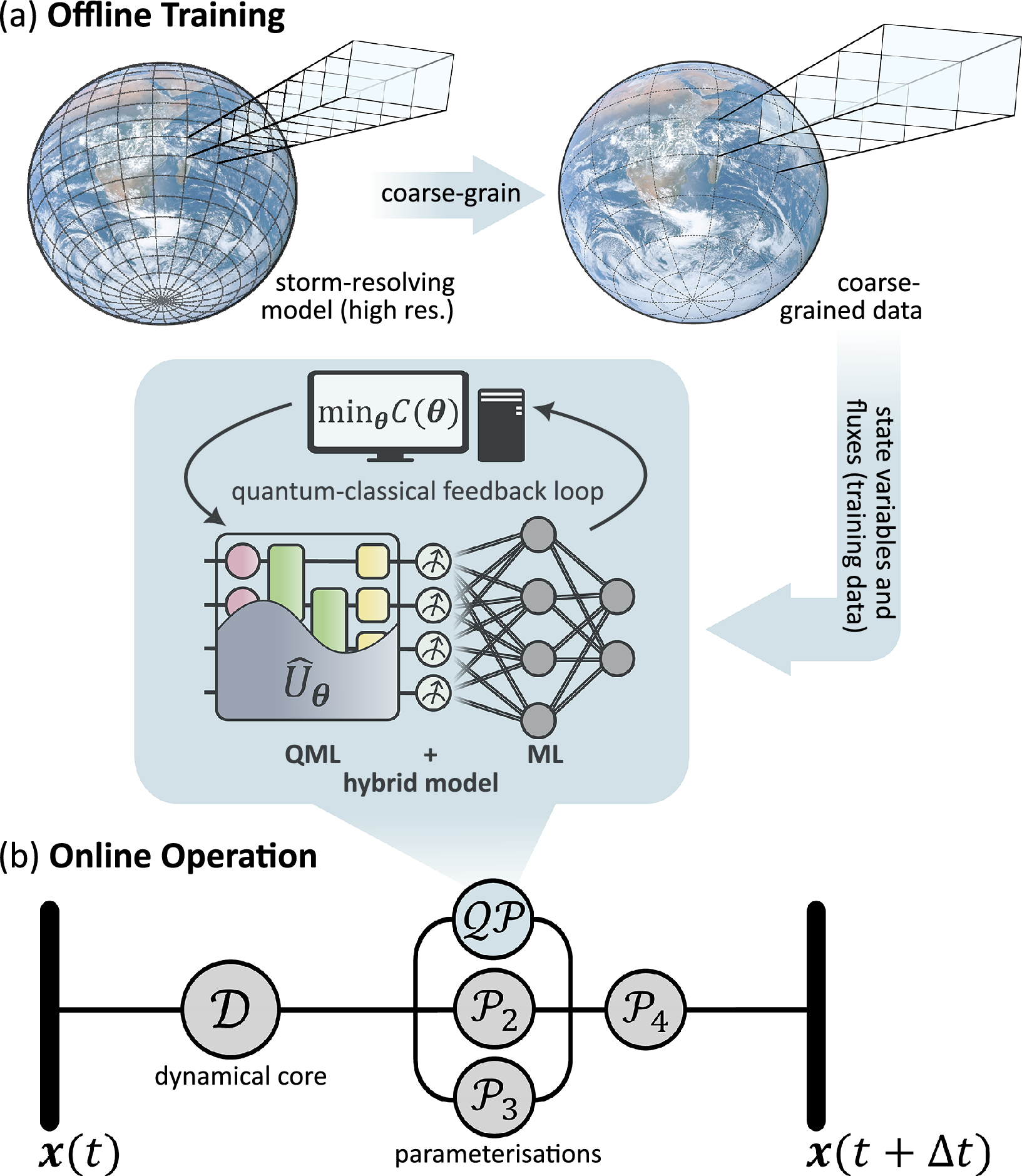
Figure 5. Hybrid quantum-classical approach for QML-based parameterizations. (a) Offline training: variables from cloud-resolving models are coarse-grained to the scale of the target climate model. The subgrid part of the variables of interest (e.g., fluxes) is calculated and used as a target for training QML-based parameterizations, possibly complemented with ML-based pre- and post-processing steps. The training of the QML model is typically assisted by a classical computer. The result is a replacement for a conventional parameterization and is coupled to the target climate model. (b) Processes occurring while the coarse-scale climate model (summarized by variables
 $ \boldsymbol{x} $
) is advanced from time step
$ \boldsymbol{x} $
) is advanced from time step
 $ t $
to
$ t $
to
 $ t+\Delta t $
. First, the dynamical core
$ t+\Delta t $
. First, the dynamical core
 $ \mathcal{D} $
is run, followed in parallel or sequentially by the various parameterizations, denoted here with
$ \mathcal{D} $
is run, followed in parallel or sequentially by the various parameterizations, denoted here with
 $ {\mathcal{P}}_2 $
to
$ {\mathcal{P}}_2 $
to
 $ {\mathcal{P}}_4 $
. The QML-parameterization
$ {\mathcal{P}}_4 $
. The QML-parameterization
 $ \mathcal{QP} $
is run online, replacing the corresponding traditional parameterization
$ \mathcal{QP} $
is run online, replacing the corresponding traditional parameterization
 $ {\mathcal{P}}_1 $
.
$ {\mathcal{P}}_1 $
.
The choice of the QNN structure is problem dependent and needs to match the hardware constraints. Also, it is desirable to encode conservation laws and physical constraints at the level of the underlying PQC, e.g., via the use of equivariant gate sets (Meyer et al., Reference Meyer, Mularski, Gil-Fuster, Mele, Arzani, Wilms and Eisert2023), or by directly encoding the physical laws into the model (Markidis, Reference Markidis2022).
Another point to consider is the probabilistic nature of the measurement outcomes. While the inherent quantum noise could prove to have some benefits for climate simulations (Tennie and Palmer, Reference Tennie and Palmer2023), the accuracy of the model prediction depends on the number of circuit evaluations, thus influencing the runtime. For nowadays’ implementations, the runtime of such QNN parameterizations constitutes a limiting factor in their usages when coupled with the climate model, since they need to be run at each time-step for all model cells. Considering a time requirement of
 $ 10\;\unicode{x03BC} \mathrm{s} $
per QNN run, and approximately
$ 10\;\unicode{x03BC} \mathrm{s} $
per QNN run, and approximately
 $ 100 $
required measurement runs (Pastori et al., Reference Pastori, Grundner, Eyring and Schwabe2025), the evaluation of a QNN parameterization for a climate model with 1 million grid cells would take
$ 100 $
required measurement runs (Pastori et al., Reference Pastori, Grundner, Eyring and Schwabe2025), the evaluation of a QNN parameterization for a climate model with 1 million grid cells would take
 $ 1000 $
s per model time-step, which is clearly prohibitive. Expected advances in quantum hardware and its coupling with HPC will also increase the potential for integrating QML routines in climate models.
$ 1000 $
s per model time-step, which is clearly prohibitive. Expected advances in quantum hardware and its coupling with HPC will also increase the potential for integrating QML routines in climate models.
4.3. Improving climate model tuning
QML models and quantum optimization routines could also be used to improve the accuracy and speed of climate model tuning following an automatic tuning procedure (Figure 6). First, the tuning goals and parameters are chosen. Then, emulators are constructed to approximate the model output and to speed up the calibration process (Bellprat et al., Reference Bellprat, Kotlarski, Lüthi and Schär2012; Watson-Parris et al., Reference Watson-Parris, Williams, Deaconu and Stier2021). Potentially optimal parameter regimes are inferred (Couvreux et al., Reference Couvreux, Hourdin, Williamson, Roehrig, Volodina, Villefranque, Rio, Audouin, Salter, Bazile, Brient, Favot, Honnert, Lefebvre, Madeleine, Rodier and Xu2021; Watson-Parris et al., Reference Watson-Parris, Williams, Deaconu and Stier2021; Allen et al., Reference Allen, Hoppel, Nedoluha, Eckermann and Barton2022; Zhang et al., Reference Zhang, Li, Lin, Xue, Xie, Xu and Huang2015; Cinquegrana et al., Reference Cinquegrana, Zollo, Montesarchio and Bucchignani2023; Bonnet et al., Reference Bonnet, Pastori, Schwabe, Giorgetta, Iglesias-Suarez and Eyring2024), and new climate model outputs are evaluated in the proposed parameter regime. The procedure is iterated until the tuning goals are achieved.
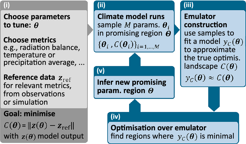
Figure 6. General steps of an automatic tuning protocol for climate models. In Step (i), the tuning goals and parameters are chosen. Then, in Step (ii) and (iii), emulators are constructed to approximate the model output and to speed up the calibration process. Potentially optimal parameter regimes are inferred in steps (iv) and (v), and new climate model outputs are evaluated in the proposed parameter regime. The procedure is iterated until the tuning goals are achieved.
The main quantum computing applications that we envision here concern the emulator construction and its optimization. Typical choices of emulators in automatic tuning schemes are neural networks and Gaussian processes (Watson-Parris et al., Reference Watson-Parris, Williams, Deaconu and Stier2021). The former choice suggests the use of QNN emulators, while the latter option implies the choice of an underlying kernel function, suggesting the use of quantum kernels in Gaussian process regression (Otten et al., Reference Otten, Goumiri, Priest, Chapline and Schneider2020). For example, Rapp and Roth (Reference Rapp and Roth2024) develop a quantum Bayesian optimization algorithm based on quantum Gaussian processes. They construct a kernel by embedding data into the Hilbert space of a quantum system
 $$ \mid \phi \left(\boldsymbol{x};\boldsymbol{\theta} \right)\left\rangle =U\left(\boldsymbol{x};\boldsymbol{\theta} \right)\mid 0\right\rangle . $$
The unitary operator
 $ U\left(\boldsymbol{x};\boldsymbol{\theta} \right) $
encodes the classical data
$ U\left(\boldsymbol{x};\boldsymbol{\theta} \right) $
encodes the classical data
 $ \boldsymbol{x} $
into a quantum state and can depend on trainable parameters
$ \boldsymbol{x} $
into a quantum state and can depend on trainable parameters
 $ \boldsymbol{\theta} $
. It implements the quantum feature map
$ \boldsymbol{\theta} $
. It implements the quantum feature map
 $ \phi $
and defines the density matrix
$ \phi $
and defines the density matrix
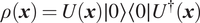 $ \rho \left(\boldsymbol{x}\right)=U\left(\boldsymbol{x}\right)\mid 0\left\rangle \right\langle 0\mid {U}^{\dagger}\left(\boldsymbol{x}\right) $
. The quantum kernel then, is given by
$ \rho \left(\boldsymbol{x}\right)=U\left(\boldsymbol{x}\right)\mid 0\left\rangle \right\langle 0\mid {U}^{\dagger}\left(\boldsymbol{x}\right) $
. The quantum kernel then, is given by
 $$ k\left(\boldsymbol{x},{\boldsymbol{x}}^{\prime}\right)=\mathrm{Tr}\left[\rho \left(\boldsymbol{x}\right)\rho \left({\boldsymbol{x}}^{\prime}\right)\right]. $$
The corresponding Gram matrix is then substituted as a covariance matrix into a classical Gaussian process, and the feature map is optimized using maximum likelihood estimation. The resulting algorithm is used for a hyperparameter optimization of a machine learning model.
Exploring the potential of QML for constructing emulators is of great interest since highly expressive models, if matched by good generalization properties, could benefit from fewer trainable parameters and training data, and hence fewer climate model simulations. The optimization of the acquisition function resulting from the emulator yields potentially optimal parameter sets and can be tackled with quantum heuristics such as quantum annealing, quantum-approximate optimization algorithms, or variational quantum eigensolvers, upon suitable discretization of the function to be optimized. Several works have recently explored the performance of these methods on continuous variable optimization problems (Izawa et al., Reference Izawa, Kitai, Tanaka, Tamura and Tsuda2022; Koh and Nishimori, Reference Koh and Nishimori2022; Abel et al., Reference Abel, Blance and Spannowsky2022). Furthermore, continuous variable quantum computers, e.g., photonic platforms, could offer alternatives to avoid parameter space discretization (Enomoto et al., Reference Enomoto, Anai, Udagawa and Takeda2023).
4.4. Assisting model analysis and evaluation
Improved climate model analysis and evaluation routines lead to better identification of climate model biases. An important task towards these goals involves learning the probability distributions underlying the models’ outputs. Classical generative methods are able to produce high-fidelity, realistic examples of climate data, e.g., with dynamics consistent with diurnal cycles (Besombes et al., Reference Besombes, Pannekoucke, Lapeyre, Sanderson and Thual2021; Behrens et al., Reference Behrens, Beucler, Gentine, Iglesias-Suarez, Pritchard and Eyring2022). Given the ability of quantum systems to efficiently, i.e., with few parameters, describe complex probability distributions (Du et al., Reference Du, Hsieh, Liu and Tao2020; Wu et al., Reference Wu, Bao, Cao, Chen, Chen, Chen, Chung, Deng, Du, Fan, Gong, Guo, Guo, Guo, Han, Hong, Huang, Huo, Li, Li, Li, Li, Liang, Lin, Lin, Qian, Qiao, Rong, Su, Sun, Wang, Wang, Wu, Xu, Yan, Yang, Yang, Ye, Yin, Ying, Yu, Zha, Zhang, Zhang, Zhang, Zhang, Zhao, Zhao, Zhou, Zhu, Lu, Peng, Zhu and Pan2021; Hangleiter and Eisert, Reference Hangleiter and Eisert2023), quantum generative models are natural candidates for achieving good extrapolating abilities using a small amount of training data. Quantum generative models can be built using PQCs, and trained either by minimizing the divergence between the target and the PQC distribution (Coyle et al., Reference Coyle, Mills, Danos and Kashefi2020) or in an adversarial manner (Dallaire-Demers and Killoran, Reference Dallaire-Demers and Killoran2018). Once trained, new samples following climate variable distributions can be efficiently generated and used for further analysis.
QML could also offer improvements in the classification of climate data, which is useful for improving and complementing observational products to subsequently use them for model evaluation (Kaps et al., Reference Kaps, Lauer, Camps-Valls, Gentine, Gomez-Chova and Eyring2023). PQCs again offer alternative ansatzes to classical ML with potential benefits (Du et al., Reference Du, Hsieh, Liu and Tao2020, Reference Du, Hsieh, Liu, You and Tao2021; Abbas et al., Reference Abbas, Sutter, Zoufal, Lucchi, Figalli and Woerner2021; Caro et al., Reference Caro, Huang, Cerezo, Sharma, Sornborger, Cincio and Coles2022). Existing QML methods for classification include quantum kernels and variants thereof (Schuld and Killoran, Reference Schuld and Killoran2019; Havlíček et al., Reference Havlíček, Córcoles, Temme, Harrow, Kandala, Chow and Gambetta2019; Huang et al., Reference Huang, Broughton, Mohseni, Babbush, Boixo, Neven and McClean2021), and QNNs (Farhi and Neven, Reference Farhi and Neven2018; Abbas et al., Reference Abbas, Sutter, Zoufal, Lucchi, Figalli and Woerner2021; Hur et al., Reference Hur, Kim and Park2022). Among these, quantum convolutional neural networks (Cong et al., Reference Cong, Choi and Lukin2019) have shown remarkable trainability and generalization capabilities when used on quantum data (Cong et al., Reference Cong, Choi and Lukin2019; Pesah et al., Reference Pesah, Cerezo, Wang, Volkoff, Sornborger and Coles2021; Du et al., Reference Du, Hsieh, Liu, You and Tao2021), although recent works have suggested the possibility of their classical simulability (Cerezo et al., Reference Cerezo, Larocca, García-Martín, Diaz, Braccia, Fontana, Rudolph, Bermejo, Ijaz, Thanasilp, Anschuetz and Holmes2023).
5. Ways ahead
Building on ML-hybrid modeling, in this perspective, we highlight the potential of quantum computing and QML to address challenges in climate modeling. The potential benefits of these applications currently come with limitations that need to be overcome, particularly concerning the short coherence times in NISQ devices, the need for an efficient coupling to HPC facilities, the large amount of data needed for typical climate applications, and the limited capacity for read-out. Nevertheless, it is crucial to start exploring the applications proposed here, to timely adapt them to future quantum devices, and to enable co-design approaches bringing together hardware engineers, software developers, and potential users in the climate modelling community. In the following, we outline some possible first steps. For each task, the role of the climate modeling community is to provide simplified problem instances and models on which routines and solvers can be tested. From the quantum side, it is crucial to identify which problems most naturally lend themselves to quantum solutions and to critically assess the potential advantages of suitable quantum algorithms. Furthermore, a task for both communities, involving also the computer science community, is to efficiently couple quantum computers and HPC facilities.
Quantum algorithms for solving partial differential equations could be applied to speed up the dynamical core of climate models. However, due to the limited read-out capacities, only few variables could be extracted from these runs. Already, with current HPC systems, it is cheaper to rerun the model if additional analyses are needed instead of storing the entire output. Quantum computers might follow this trend to an extreme degree, resulting in only a very limited output for each run, but repeating the runs a large number of times. In the near future, work could be started by solving simple equations such as the 1D shallow water equations, followed by adapting simplified climate models for quantum computers using only a few grid points, vertical levels, and prognostic variables.
Another, potentially near-term, use of quantum computers is to improve subgrid-scale parameterizations. Running QML-based parameterizations coupled to the climate model requires considerable quantum and classical runtime with overheads due to the quantum-classical coupling, since the quantum computer needs to run the QML parameterization. Recently proposed options that could help circumvent this challenge are surrogates or shadows of QML models (Schreiber et al., Reference Schreiber, Eisert and Meyer2023; Jerbi et al., Reference Jerbi, Gyurik, Marshall, Molteni and Dunjko2024). These are classical models emulating the outputs of previously trained QML models, thus potentially retaining some of the potential benefits while requiring a quantum device only during the training stage.
Tuning the free parameters of a climate model is a very time-consuming process that could be improved using quantum-assisted automatic routines. A first step towards developing an automatic calibration method could be tuning the Lorenz-96 model (Lorenz, Reference Lorenz, Palmer and Hagedorn2006), which resembles the non-linear behavior of the climate system (Mouatadid et al., Reference Mouatadid, Gentine, Yu and Easterbrook2019).
Finally, for the analysis and evaluation of the resulting models, QML methods could provide potentially better classification of climate data, and alternative generative models efficiently reproduce realistic distributions of climate variables. The first steps for this would be to adapt the existing small-scale applications of quantum classifiers (Schuld and Killoran, Reference Schuld and Killoran2019; Havlíček et al., Reference Havlíček, Córcoles, Temme, Harrow, Kandala, Chow and Gambetta2019; Huang et al., Reference Huang, Broughton, Mohseni, Babbush, Boixo, Neven and McClean2021; Farhi and Neven, Reference Farhi and Neven2018; Abbas et al., Reference Abbas, Sutter, Zoufal, Lucchi, Figalli and Woerner2021; Hur et al., Reference Hur, Kim and Park2022) and quantum generative models (Coyle et al., Reference Coyle, Mills, Danos and Kashefi2020; Dallaire-Demers and Killoran, Reference Dallaire-Demers and Killoran2018; Zoufal et al., Reference Zoufal, Lucchi and Woerner2019) to climate data, e.g., to simplified cloud classification problems.
All these research efforts are still in their infancy and face numerous challenges. Nevertheless, they offer exciting potential to significantly boost climate modelling to allow more robust regional climate projections and thus help manage the challenge posed by climate change, in addition to current efforts on hybrid ESMs (Eyring et al., Reference Eyring, Gentine, Camps-Valls, Lawrence and Reichstein2024b) and high resolution modelling (Stevens et al., Reference Stevens, Adami, Ali, Anzt, Aslan, Attinger, Bäck, Baehr, Bauer, Bernier, Bishop, Bockelmann, Bony, Brasseur, Bresch, Breyer, Brunet, Buttigieg, Cao, Castet, Cheng, Dey Choudhury, Coen, Crewell, Dabholkar, Dai, Doblas-Reyes, Durran, El Gaidi, Ewen, Exarchou, Eyring, Falkinhoff, Farrell, Forster, Frassoni, Frauen, Fuhrer, Gani, Gerber, Goldfarb, Grieger, Gruber, Hazeleger, Herken, Hewitt, Hoefler, Hsu, Jacob, Jahn, Jakob, Jung, Kadow, Kang, Kang, Kashinath, Kleinen-von Königslöw, Klocke, Kloenne, Klöwer, Kodama, Kollet, Kölling, Kontkanen, Kopp, Koran, Kulmala, Lappalainen, Latifi, Lawrence, Lee, Lejeun, Lessig, Li, Lippert, Luterbacher, Manninen, Marotzke, Matsouoka, Merchant, Messmer, Michel, Michielsen, Miyakawa, Müller, Munir, Narayanasetti, Ndiaye, Nobre, Oberg, Oki, Özkan Haller, Palmer, Posey, Prein, Primus, Pritchard, Pullen, Putrasahan, Quaas, Raghavan, Ramaswamy, Rapp, Rauser, Reichstein, Revi, Saluja, Satoh, Schemann, Schemm, Schnadt Poberaj, Schulthess, Senior, Shukla, Singh, Slingo, Sobel, Solman, Spitzer, Stier, Stocker, Strock, Su, Taalas, Taylor, Tegtmeier, Teutsch, Tompkins, Ulbrich, Vidale, Wu, Xu, Zaki, Zanna, Zhou and Ziemen2024).
Open peer review
To view the open peer review materials for this article, please visit http://doi.org/10.1017/eds.2025.10010.
Author contribution
Conceptualization: M.S., V.E., L.P. Visualization: L.P., M.S. Writing original draft: M.S., L.P., I.d.V., P.G., L.I., V.L., M.L., J.M.L., V.E. All authors approved the final submitted draft.
Competing interests
None.
Data availability statement
No data were used in this position paper.
Ethics statement
The research meets all ethical guidelines, including adherence to the legal requirements of the study country.
Funding statement
This project was made possible by the DLR Quantum Computing Initiative and the Federal Ministry for Economic Affairs and Climate Action; qci.dlr.de/projects/klim-qml. Funding for this study was also provided by the European Research Council (ERC) Synergy Grant “Understanding and Modelling the Earth System with Machine Learning (USMILE)” under the Horizon 2020 research and innovation programme (Grant agreement No. 855187). V.E. was additionally supported by the Deutsche Forschungsgemeinschaft (DFG, German Research Foundation) through the Gottfried Wilhelm Leibniz Prize awarded to Veronika Eyring (Reference No. EY 22/2-1). The research by L.I. and J.M.L. is partially funded in the context of the Munich Quantum Valley, which is supported by the Bavarian state government with funds from the Hightech Agenda Bayern Plus.


 Open access
Comments
Dear Environmental Data Science editors,
thank you for accepting my proposal to submit a Position Paper on Quantum computing to improve
and accelerate climate models (email from 14 October). I hereby submit the paper entitled “Opportunities and challenges of quantum computing for climate modelling” for your consideration. In this paper, we discuss potential applications of quantum computing for climate models, e.g., to improve parameterizations with QML, accelerate the solution of the underlying differential equations, and help with tuning climate models. We include an introduction to the methods and a discussion of challenges.
We believe that this paper fits very well within the scope of Environmental Data Science and will serve to stimulate the research in the intersection of the two areas of quantum computing and climate science.
We look forward to hearing from you.
Best regards,
On behalf of the authors,
Mierk Schwabe