


1 Introduction
In [Reference Furstenberg and WeissFW03] Furstenberg and Weiss initiated the use of dynamical methods in the study of Ramsey theoretic questions for trees. They proved a Szemerédi-type theorem using a multiple recurrence result for a class of Markov processes (a purely combinatorial proof was later given by Pach, Solymosi and Tardos [Reference Pach, Solymosi and TardosPST12]). More precisely, they showed that finite replicas of the full binary tree could always be found in (infinite) trees of positive growth rate. It is then a natural question to quantify the abundance of finite configurations in a tree in relation to its size as measured by its upper Minkowski and Hausdorff dimensions.
To begin, we review the analogous question in the integer setting. Specifically, we consider the abundance of configurations in a subset
 $E \subset \mathbb {N}$
. Recall that the upper density and upper Banach density of E are
$E \subset \mathbb {N}$
. Recall that the upper density and upper Banach density of E are
 $$ \begin{align*} \overline{d}(E) = \limsup_{N \to \infty} \frac{|E \cap \{0,\ldots,N\}|}{N+1}, \quad d^{\ast}(E) = \limsup_{N-M \to \infty} \frac{|E \cap \{M,\ldots,N\}|}{N-M+1}. \end{align*} $$
The abundance of
 $2$
-term arithmetic progressions (2-APs) in E can be related to the density of E in the following way. Consider the sets of popular differences of E with respect to
$2$
-term arithmetic progressions (2-APs) in E can be related to the density of E in the following way. Consider the sets of popular differences of E with respect to
 $\overline {d}$
and
$\overline {d}$
and
 $d^{\ast }$
defined by
$d^{\ast }$
defined by
 $$ \begin{align*} \overline{\Delta}_0(E) = \{n \in \mathbb{N} \colon \overline{d}(E \cap (E-n))>0\}, \quad \Delta_0^{\ast}(E) = \{n \in \mathbb{N} \colon d^{\ast}(E \cap (E-n))>0\}. \end{align*} $$
Furstenberg’s correspondence principle [Reference FurstenbergFur77] states that there exists a measure- preserving system
 $(X,\mathscr {B},\nu ,S)$
and
$(X,\mathscr {B},\nu ,S)$
and
 $A \in \mathscr {B}$
with
$A \in \mathscr {B}$
with
 $\nu (A) = \overline {d}(E)$
such that for all integers
$\nu (A) = \overline {d}(E)$
such that for all integers
 $k \geqslant 1$
and
$k \geqslant 1$
and
 $0=n_1,\ldots ,n_k \in \mathbb {N}$
,
$0=n_1,\ldots ,n_k \in \mathbb {N}$
,
 $$ \begin{align*} \overline{d}((E-n_1) \cap \cdots \cap (E-n_k)) \geqslant \nu(S^{-n_1}A \cap \cdots \cap S^{-n_k}A). \end{align*} $$
Taking
 $k=2$
, it follows that
$k=2$
, it follows that
 $\overline {\Delta }_0(E)$
contains
$\overline {\Delta }_0(E)$
contains
 $$ \begin{align*} \mathcal{R}=\mathcal{R}(A) = \{n \in \mathbb{N} \colon \nu(A \cap S^{-n}A)>0\}, \end{align*} $$
the set of return times of A. Applying the mean ergodic theorem then gives
 $$ \begin{align} \underline{d}(\overline{\Delta}_0(E)) \geqslant \underline{d}(\mathcal{R}) \geqslant \lim_{N \to \infty} \frac{1}{N+1} \sum_{n=0}^{N}\frac{\nu(A \cap S^{-n}A)}{\nu(A)} \geqslant \nu(A) = \overline{d}(E), \end{align} $$
where the lower density
 $\underline {d}$
is defined for
$\underline {d}$
is defined for
 $E \subset \mathbb {N}$
by
$E \subset \mathbb {N}$
by
 $$ \begin{align*} \underline{d}(E) = \liminf_{N \to \infty} \frac{|E \cap \{0,\ldots,N\}|}{N+1}. \end{align*} $$
If in the above the upper density is replaced by the upper Banach density, then
 $\nu $
can further be chosen to be ergodic [Reference FurstenbergFur81, Proposition 3.9] (see [Reference Bergelson, Host and KraBHK05, Proposition 3.1] for an explicit proof).
$\nu $
can further be chosen to be ergodic [Reference FurstenbergFur81, Proposition 3.9] (see [Reference Bergelson, Host and KraBHK05, Proposition 3.1] for an explicit proof).
Following Furstenberg and Weiss [Reference Furstenberg and WeissFW03], we formulate a correspondence principle for arbitrary finite configurations in a tree and use it to obtain analogues of the inequality (1). We then analyze the case of equality in (1) and its analogues for trees using inverse theorems for the set of return times. In the ergodic situation we use a result of Björklund, the first author and Shkredov [Reference Björklund, Fish and ShkredovBFS21] and a stability-type extension proved jointly with Shkredov in Appendix A, whereas in the general case we prove a slightly weaker statement (Theorem 5.1). Using these, we obtain inverse theorems for inequality (1): a tree for which equality holds must contain arbitrarily long ‘arithmetic progressions’ with a fixed common difference.
1.1 Main results
To describe our results, we first summarize the necessary definitions (see §2 for precise formulations). For clarity of exposition, in this introduction we restrict our attention to the case
 $r=2$
of our results and make corresponding simplifications to the notation.
$r=2$
of our results and make corresponding simplifications to the notation.
Fix an integer
 $q \geqslant 2$
. In this paper, a tree can be visualized as a directed graph T with a distinguished vertex (the root) having no incoming edges, such that each vertex has between
$q \geqslant 2$
. In this paper, a tree can be visualized as a directed graph T with a distinguished vertex (the root) having no incoming edges, such that each vertex has between
 $1$
and q outgoing edges and each non-root vertex has exactly one incoming edge. (Technically, we work with the vertices of the graph with the partial order induced by directed paths.) The ‘size’ of T can be quantified by its upper Minkowski and Hausdorff dimensions
$1$
and q outgoing edges and each non-root vertex has exactly one incoming edge. (Technically, we work with the vertices of the graph with the partial order induced by directed paths.) The ‘size’ of T can be quantified by its upper Minkowski and Hausdorff dimensions
 $\overline {\dim }_MT$
and
$\overline {\dim }_MT$
and
 $\dim T$
, which are defined by an identification of such trees with closed subsets of
$\dim T$
, which are defined by an identification of such trees with closed subsets of
 $[0,1]$
.
$[0,1]$
.
1.1.1 Tree analogues of popular difference sets
A k-term arithmetic progression (k-AP) in
 $E \subset \mathbb {N}$
can be viewed as an affine map
$E \subset \mathbb {N}$
can be viewed as an affine map
 $\{0,\ldots ,k-1\} \to E$
. We consider ‘affine’ maps satisfying certain branching conditions from configurations C (‘finite trees’) to trees T. If there exists such a map with ‘common difference’ n taking the root of the configuration to
$\{0,\ldots ,k-1\} \to E$
. We consider ‘affine’ maps satisfying certain branching conditions from configurations C (‘finite trees’) to trees T. If there exists such a map with ‘common difference’ n taking the root of the configuration to
 $v \in T$
, we say that
$v \in T$
, we say that
 $v \in C_n = C_n(T)$
. The set
$v \in C_n = C_n(T)$
. The set
 $C_n$
corresponds to the set
$C_n$
corresponds to the set
 $E \cap (E-n) \cap \cdots \cap (E-(k-1)n)$
for k-APs in
$E \cap (E-n) \cap \cdots \cap (E-(k-1)n)$
for k-APs in
 $E \subset \mathbb {N}$
. Using extensions of upper density and upper Banach density to subsets of trees, we define sets of ‘generic parameters’
$E \subset \mathbb {N}$
. Using extensions of upper density and upper Banach density to subsets of trees, we define sets of ‘generic parameters’
 $$ \begin{align*} \overline{G}(C) = \{n \in \mathbb{N} \colon \overline{d}(C_n)> 0 \}, \quad G^{\ast}(C) = \{n \in \mathbb{N} \colon d^{\ast}(C_n) > 0 \}. \end{align*} $$
We also introduce certain configurations F and D which are analogues of
 $2$
-APs, and their generic parameters can be interpreted as popular differences for trees. In particular, our first result is a version of (1).
$2$
-APs, and their generic parameters can be interpreted as popular differences for trees. In particular, our first result is a version of (1).
Theorem A. (= Theorems 4.1 and 4.2 for
 $r=2$
)
$r=2$
)

For any tree T we have
 $$ \begin{align*}\underline{d}(\overline{G}(F)) \geqslant \underline{d}(\overline{G}(D)) \geqslant \overline{\dim}_M T \quad \text{and} \quad \underline{d}(G^{\ast}(F)) \geqslant \underline{d}(G^{\ast}(D)) \geqslant \dim T.\end{align*} $$
1.1.2 Inverse theorems for sets of return times
Given the direct result Theorem A, we are interested in characterizing trees such that equality holds (or almost holds). To illustrate the ideas, we consider here the situation when equality is (almost) achieved in (1), which is the analogous question for subsets of
 $\mathbb {N}$
. Observe that the density of the set of return times of A is then close to the measure of A. It is natural to expect in this situation that the dynamics of A under S is rigid in some way, and this is indeed the case.
$\mathbb {N}$
. Observe that the density of the set of return times of A is then close to the measure of A. It is natural to expect in this situation that the dynamics of A under S is rigid in some way, and this is indeed the case.
Let
 $(X,\mathscr {B},\nu ,S)$
be a measure-preserving system, and let A be a measurable set with
$(X,\mathscr {B},\nu ,S)$
be a measure-preserving system, and let A be a measurable set with
 $\nu (A)> 0$
and set of return times
$\nu (A)> 0$
and set of return times
 $\mathcal {R}$
. Using a theorem of Kneser we prove the following result.
$\mathcal {R}$
. Using a theorem of Kneser we prove the following result.
Theorem B. (= Theorem 5.1)
If
 $\overline {d}(\mathcal {R}) = \nu (A)> 0$
, then there exists an integer
$\overline {d}(\mathcal {R}) = \nu (A)> 0$
, then there exists an integer
 $m \geqslant 1$
such that up to
$m \geqslant 1$
such that up to
 $\nu $
-null sets
$\nu $
-null sets
 $$ \begin{align*}X = \bigsqcup_{i=0}^{m-1} S^{-i} A. \end{align*} $$
Question 1.1. Does the assumption
 $\underline {d}(\mathcal {R}) = \nu (A)$
suffice to prove the conclusion of Theorem B?
$\underline {d}(\mathcal {R}) = \nu (A)$
suffice to prove the conclusion of Theorem B?
If
 $\nu $
is ergodic, then Question 1.1 has an affirmative answer, and further there is an inverse result for cases of almost equality. The following theorem is an easy corollary of results by Björklund, the first author and Shkredov in [Reference Björklund, Fish and ShkredovBFS21].
$\nu $
is ergodic, then Question 1.1 has an affirmative answer, and further there is an inverse result for cases of almost equality. The following theorem is an easy corollary of results by Björklund, the first author and Shkredov in [Reference Björklund, Fish and ShkredovBFS21].
Theorem 1.2. (= Theorem 5.4)
If
 $(X,\mathscr {B},\nu ,S)$
is ergodic and
$(X,\mathscr {B},\nu ,S)$
is ergodic and
 $$ \begin{align*} 0 < \underline{d}(\mathcal{R}) < \tfrac{3}{2} \nu(A), \end{align*} $$
then there exists an integer
 $m \geqslant 1$
such that
$m \geqslant 1$
such that
 $\mathcal {R} = m \mathbb {N}$
and
$\mathcal {R} = m \mathbb {N}$
and
 $X = \bigsqcup _{i=0}^{m-1} S^{-i}( \bigcup _{j=0}^{\infty }S^{-jm} A )$
up to
$X = \bigsqcup _{i=0}^{m-1} S^{-i}( \bigcup _{j=0}^{\infty }S^{-jm} A )$
up to
 $\nu $
-null sets.
$\nu $
-null sets.
Remark 1.3. Example 1.2 in [Reference Björklund, Fish and ShkredovBFS21] shows that for every
 $\beta> 1$
, there exists a non-ergodic measure-preserving system
$\beta> 1$
, there exists a non-ergodic measure-preserving system
 $(X,\mathscr {B},\nu ,S)$
and
$(X,\mathscr {B},\nu ,S)$
and
 $A \in \mathscr {B}$
of arbitrarily small measure such that
$A \in \mathscr {B}$
of arbitrarily small measure such that
 $\overline {d}(\mathcal {R}) \leqslant \beta \nu (A)$
and there is no
$\overline {d}(\mathcal {R}) \leqslant \beta \nu (A)$
and there is no
 $m \geqslant 1$
such that
$m \geqslant 1$
such that
 $\mathcal {R} = m\mathbb {N}$
.
$\mathcal {R} = m\mathbb {N}$
.
1.1.3 Inverse results for popular difference sets
As a corollary of Theorem B and Furstenberg’s correspondence principle, we immediately obtain the following inverse-type result for (1).
Proposition 1.4. Assume that
 $E \subset \mathbb {N}$
satisfies
$E \subset \mathbb {N}$
satisfies
 $\overline {d}(\overline {\Delta }_0(E)) = \overline {d}(E)>0$
. Then there exists
$\overline {d}(\overline {\Delta }_0(E)) = \overline {d}(E)>0$
. Then there exists
 $m \geqslant 1$
such that
$m \geqslant 1$
such that
 $m \mathbb {N} \subset \overline {\Delta }_0(E)$
and
$m \mathbb {N} \subset \overline {\Delta }_0(E)$
and
 $\overline {d}(\overline {\Delta }_0(E)) = \overline {d}(E) = m^{-1}$
. Moreover, for every
$\overline {d}(\overline {\Delta }_0(E)) = \overline {d}(E) = m^{-1}$
. Moreover, for every
 $k \geqslant 2$
 $$ \begin{align*} \overline{d}( E \cap (E-m) \cap \cdots \cap (E- (k-1)m) ) = \overline{d}(E). \end{align*} $$
If we consider
 $\Delta ^{\ast }_0(E)$
and
$\Delta ^{\ast }_0(E)$
and
 $d^{\ast }(E)$
in place of
$d^{\ast }(E)$
in place of
 $\overline {\Delta }_0(E)$
and
$\overline {\Delta }_0(E)$
and
 $\overline {d}(E)$
, we can apply Theorem 1.2 to obtain the following inverse result.
$\overline {d}(E)$
, we can apply Theorem 1.2 to obtain the following inverse result.
Proposition 1.5. Let
 $1 \leqslant \beta < 3/2$
. Assume that
$1 \leqslant \beta < 3/2$
. Assume that
 $E \subset \mathbb {N}$
satisfies
$E \subset \mathbb {N}$
satisfies
 $$ \begin{align*}0 < \underline{d}(\Delta^{\ast}_0(E)) = \beta \cdot d^{\ast}(E). \end{align*} $$
Then there exists
 $m \geqslant 1$
such that
$m \geqslant 1$
such that
 $m \mathbb {N} \subset \Delta ^{\ast }_0(E)$
. Moreover, for every
$m \mathbb {N} \subset \Delta ^{\ast }_0(E)$
. Moreover, for every
 $k \geqslant 2$
that satisfies
$k \geqslant 2$
that satisfies
 $(1 - \beta ^{-1})k < 1$
, we have
$(1 - \beta ^{-1})k < 1$
, we have
 $$ \begin{align*} d^{\ast}(E \cap (E-m) \cap \cdots \cap (E- (k-1)m))> 0. \end{align*} $$
1.1.4 Inverse results for
$\overline {G}(F)$
and
$G^{\ast }(F)$


Propositions 1.4 and 1.5 can be interpreted as saying that (almost) equality holds in (1) for a subset
 $E \subset \mathbb {N}$
only if E is ‘similar’ to the periodic set
$E \subset \mathbb {N}$
only if E is ‘similar’ to the periodic set
 $m\mathbb {N}$
. In the tree setting, we prove analogous results.
$m\mathbb {N}$
. In the tree setting, we prove analogous results.
For every
 $m \geqslant 1$
, define
$m \geqslant 1$
, define
 $T_{m\mathbb {N}}$
to be the tree such that
$T_{m\mathbb {N}}$
to be the tree such that
 $v \in T_{m\mathbb {N}}$
has q outgoing edges if the directed path from the root to v has length a multiple of m and one outgoing edge otherwise. The inequalities in Theorem A are equalities for
$v \in T_{m\mathbb {N}}$
has q outgoing edges if the directed path from the root to v has length a multiple of m and one outgoing edge otherwise. The inequalities in Theorem A are equalities for
 $T_{m\mathbb {N}}$
(see §2.1.1).
$T_{m\mathbb {N}}$
(see §2.1.1).
For every
 $k \geqslant 1$
, define the configuration
$k \geqslant 1$
, define the configuration
 $V^{m,k}$
to be the first k levels of
$V^{m,k}$
to be the first k levels of
 $T_{m\mathbb {N}}$
. The following two theorems are analogues of Propositions 1.4 and 1.5, respectively.
$T_{m\mathbb {N}}$
. The following two theorems are analogues of Propositions 1.4 and 1.5, respectively.
Theorem C. (= Theorem 6.1 for
$r=2$
)

Let T be a tree. Assume that
 $$ \begin{align*}\overline{d}(\overline{G}(F)) = \overline{\dim}_M T> 0. \end{align*} $$
Then there exists an integer
 $m \geqslant 1$
such that
$m \geqslant 1$
such that
 $\overline {\dim }_M T = m^{-1}$
, and
$\overline {\dim }_M T = m^{-1}$
, and
 $\overline {d}(V^{m,k})> 0$
for every
$\overline {d}(V^{m,k})> 0$
for every
 $k \geqslant 1$
.
$k \geqslant 1$
.
Theorem D. (= Theorem 6.2 for
$r=2$
)

Let T be a tree. Assume that
 $$ \begin{align*} \underline{d}(G^{\ast}(F)) = \dim T> 0 \quad \text{or} \quad \overline{d}(G^{\ast}(D)) = \dim T > 0. \end{align*} $$
Then there exists an integer
 $m \geqslant 1$
such that
$m \geqslant 1$
such that
 $\dim T = m^{-1}$
, and
$\dim T = m^{-1}$
, and
 $d^{\ast }(V^{m,k})> 0$
for every
$d^{\ast }(V^{m,k})> 0$
for every
 $k \geqslant 1$
.
$k \geqslant 1$
.
Remark 1.6. We show in §2.1.2 that Theorem D cannot be improved. Indeed, for every
 $\varepsilon> 0$
there exists a tree
$\varepsilon> 0$
there exists a tree
 $T_{\varepsilon }$
such that
$T_{\varepsilon }$
such that
 $$ \begin{align*} 0 < \dim T_{\varepsilon} \leqslant \underline{d}(G^{\ast}(F)) < (1+\varepsilon) \dim T_{\varepsilon} \end{align*} $$
and the configuration
 $V^{m,k}$
does not appear at all in
$V^{m,k}$
does not appear at all in
 $T_{\varepsilon }$
for some large k.
$T_{\varepsilon }$
for some large k.
Our final result is another partial analogue of Proposition 1.5.
Theorem 1.7. (= Theorem 6.4 for
$r=2$
)

Let T be a tree. Assume that there exists
 ${\beta < 3/2}$
such that
${\beta < 3/2}$
such that
 $$ \begin{align*} 0 < \underline{d}(G^{\ast}(F)) = \beta \cdot \dim T. \end{align*} $$
Then there exists
 $m \geqslant 1$
with
$m \geqslant 1$
with
 $m \mathbb {N} \subset G^{\ast }(F)$
.
$m \mathbb {N} \subset G^{\ast }(F)$
.
1.2 Organization of the paper
After describing the combinatorial and dynamical background (§2) and establishing Furstenberg–Weiss correspondence principles (§3), in §4 we prove lower bounds for the densities of popular differences for trees. We then use inverse theorems for sets of return times in measure-preserving systems (§5 and Appendix A) to prove inverse theorems for these lower bounds (§6).
2 Trees and Markov processes
Fix an integer
 $q \geqslant 2$
, and for
$q \geqslant 2$
, and for
 $2 \leqslant r \leqslant q$
define
$2 \leqslant r \leqslant q$
define
 $\Lambda _r = \{0,\ldots ,r-1\}$
and
$\Lambda _r = \{0,\ldots ,r-1\}$
and
 $\Lambda = \Lambda _q$
. We set
$\Lambda = \Lambda _q$
. We set
 $\mathbb {N} = \{0,1,\ldots \}$
.
$\mathbb {N} = \{0,1,\ldots \}$
.
2.1 Combinatorial setup
Let
 $\Lambda ^{\ast } = \bigcup _{n=0}^{\infty } \Lambda ^n$
be the set of finite words over
$\Lambda ^{\ast } = \bigcup _{n=0}^{\infty } \Lambda ^n$
be the set of finite words over
 $\Lambda $
, where
$\Lambda $
, where
 $\Lambda ^0$
is the singleton comprising the empty word
$\Lambda ^0$
is the singleton comprising the empty word
 $\emptyset $
. Consider the partial order
$\emptyset $
. Consider the partial order
 $\leqslant $
on
$\leqslant $
on
 $\Lambda ^{\ast }$
defined by
$\Lambda ^{\ast }$
defined by
 $v \leqslant w$
if w is the concatenation
$v \leqslant w$
if w is the concatenation
 $vu$
of v and some
$vu$
of v and some
 $u \in \Lambda ^{\ast }$
. A tree is then a non-empty subset
$u \in \Lambda ^{\ast }$
. A tree is then a non-empty subset
 $T \subset \Lambda ^{\ast }$
closed under predecessors and having no maximal elements with respect to
$T \subset \Lambda ^{\ast }$
closed under predecessors and having no maximal elements with respect to
 $\leqslant $
. We refer to elements of T as vertices (using the natural graph-theoretic terminology), and write
$\leqslant $
. We refer to elements of T as vertices (using the natural graph-theoretic terminology), and write
 $l(v)=n$
if
$l(v)=n$
if
 $v \in T(n) = T \cap \Lambda ^n$
. Every tree contains
$v \in T(n) = T \cap \Lambda ^n$
. Every tree contains
 $\emptyset $
(the root), and for every
$\emptyset $
(the root), and for every
 $v \in T$
there is a tree
$v \in T$
there is a tree
 $T^v = \{w \in \Lambda ^{\ast } \colon vw \in T\}$
.
$T^v = \{w \in \Lambda ^{\ast } \colon vw \in T\}$
.
Remark 2.1. Trees are combinatorial realizations of closed sets in
 $\Lambda ^{\mathbb {N}}$
, a symbolic analogue of
$\Lambda ^{\mathbb {N}}$
, a symbolic analogue of
 $[0,1]$
. Given a tree T, the set
$[0,1]$
. Given a tree T, the set
 $$ \begin{align*}\{(a_i)_{i\geqslant 0} \in \Lambda^{\mathbb{N}} \colon (a_0,\ldots,a_n) \in T \text{ for all }n \in \mathbb{N}\}\end{align*} $$
is closed in
 $\Lambda ^{\mathbb {N}}$
(with the product of discrete topologies on
$\Lambda ^{\mathbb {N}}$
(with the product of discrete topologies on
 $\Lambda $
), and there is an inverse map sending a closed subset
$\Lambda $
), and there is an inverse map sending a closed subset
 $A \subset \Lambda ^{\mathbb {N}}$
to the tree
$A \subset \Lambda ^{\mathbb {N}}$
to the tree
 $$ \begin{align*} \{v \in \Lambda^{\ast} \colon vw \in A \text{ for some }w \in \Lambda^{\mathbb{N}}\}. \end{align*} $$
This motivates several definitions we give in the following.
The (upper) Minkowski dimension of T is
 $$ \begin{align*} \overline{\dim}_M T = \limsup_{N \to \infty} \frac{\log_q|T(N)|}{N}. \end{align*} $$
To define the Hausdorff dimension of a tree, we first define the analogue of an irredundant open cover for trees. A section of a tree T is a finite subset
 $\Pi \subset T$
such that
$\Pi \subset T$
such that
 $|\Pi \cap \{w \in T \colon w \leqslant v\}|=1$
for all but finitely many
$|\Pi \cap \{w \in T \colon w \leqslant v\}|=1$
for all but finitely many
 $v \in T$
. Define also
$v \in T$
. Define also
 $l(\Pi ) = \min \{l(v) \colon v \in \Pi \}$
. Then the Hausdorff dimension of T is
$l(\Pi ) = \min \{l(v) \colon v \in \Pi \}$
. Then the Hausdorff dimension of T is
 $$ \begin{align*} \dim T = \inf \bigg\{ \unicode{x3bb}>0 \colon \liminf_{N \to \infty} \inf_{\substack{l(\Pi)=N \\ \Pi \text{ section of } T}} \sum_{v \in \Pi} q^{-\unicode{x3bb} l(v)} < 1\bigg\}. \end{align*} $$
Example 2.2. Given
 $E \subset \mathbb {N}$
and
$E \subset \mathbb {N}$
and
 $2 \leqslant r \leqslant q$
, define the tree
$2 \leqslant r \leqslant q$
, define the tree
 $$ \begin{align*} T_E^r = \{\emptyset\} \cup \bigcup_{i=0}^{\infty} \prod_{0 \leqslant j \leqslant i} \Gamma_j \quad \text{ where } \Gamma_j = \begin{cases} \Lambda & \text{ if } j \in E, \\ \Lambda_{r-1} & \text{ otherwise.} \end{cases} \end{align*} $$
A straightforward calculation shows that
 $$ \begin{align*} \overline{\dim}_M T_E^r &= \limsup_{N \to \infty} \frac{\log_q { q^{|E \cap \{0,\ldots,N-1\}|} (r-1)^{|E^c \cap \{0,\ldots,N -1\}|}}}{N} \\ &= \overline{d}(E) + \log_q (r-1) (1 - \overline{d}(E)). \end{align*} $$
If E is a ‘periodic’ set (such as
 $m\mathbb {N}$
), then
$m\mathbb {N}$
), then
 $T_E^r$
is ‘self-similar’ and
$T_E^r$
is ‘self-similar’ and
 $\overline {\dim }_M T_E^r = \dim T_E^r$
.
$\overline {\dim }_M T_E^r = \dim T_E^r$
.
Elements of
 $\Lambda ^{\ast }$
correspond to cylinder sets of
$\Lambda ^{\ast }$
correspond to cylinder sets of
 $\Lambda ^{\mathbb {N}}$
. By the Carathéodory extension theorem, Borel probability measures on
$\Lambda ^{\mathbb {N}}$
. By the Carathéodory extension theorem, Borel probability measures on
 $\Lambda ^{\mathbb {N}}$
are in bijection with functions
$\Lambda ^{\mathbb {N}}$
are in bijection with functions
 $\tau \colon \Lambda ^{\ast } \to [0,1]$
such that
$\tau \colon \Lambda ^{\ast } \to [0,1]$
such that
 $\tau (\emptyset ) = 1$
and
$\tau (\emptyset ) = 1$
and
 $\tau (v) = \sum _{a \in \Lambda } \tau (va)$
for all
$\tau (v) = \sum _{a \in \Lambda } \tau (va)$
for all
 $v \in \Lambda ^{\ast }$
. We call such functions Markov trees, because the support
$v \in \Lambda ^{\ast }$
. We call such functions Markov trees, because the support
 $|\tau | = \{v \in \Lambda ^{\ast } \colon \tau (v)>0\}$
of such a function is a tree. The set of Markov trees is a closed subspace of the compact space
$|\tau | = \{v \in \Lambda ^{\ast } \colon \tau (v)>0\}$
of such a function is a tree. The set of Markov trees is a closed subspace of the compact space
 $[0,1]^{\Lambda ^{\ast }}$
with metric
$[0,1]^{\Lambda ^{\ast }}$
with metric
 $d(\tau _1,\tau _2) = \sum _{v \in \Lambda ^{\ast }} q^{-l(v)}|\tau _1(v)-\tau _2(v)|$
. By abuse of notation we denote it by
$d(\tau _1,\tau _2) = \sum _{v \in \Lambda ^{\ast }} q^{-l(v)}|\tau _1(v)-\tau _2(v)|$
. By abuse of notation we denote it by
 $\mathcal {P}(\Lambda ^{\mathbb {N}})$
, because it is homeomorphic to the space of Borel probability measures on
$\mathcal {P}(\Lambda ^{\mathbb {N}})$
, because it is homeomorphic to the space of Borel probability measures on
 $\Lambda ^{\mathbb {N}}$
with the weak-
$\Lambda ^{\mathbb {N}}$
with the weak-
 ${}^{\ast }$
topology.
${}^{\ast }$
topology.
The dimension of a Markov tree [Reference FurstenbergFur70, Definition 7] is
 $$ \begin{align*}\dim \tau = \liminf_{\substack{l(\Pi)\to\infty \\ \Pi \text{ section of } |\tau|}} \frac{-\sum_{v \in \Pi} \tau(v)\log_q \tau(v)}{\sum_{v \in \Pi}l(v)\tau(v)}.\end{align*} $$
Given a subset
 $V \subset T$
, we define its upper density
$V \subset T$
, we define its upper density
 $$ \begin{align*} \overline{d}(V) = \limsup_{N \to \infty} \frac{1}{|T(N)|} \sum_{v \in T(N)} \frac{|V \cap \{w \in T \colon w \leqslant v\}|}{N+1} \end{align*} $$
and its upper Banach density
 $$ \begin{align*}d^{\ast}(V) = \limsup_{N \to \infty} \sup_{\substack{|\tau| \subset T \\ v \in |\tau|}} \frac{1}{N+1} \sum_{l(w) \leqslant N} \frac{\tau(vw)}{\tau(v)}1_V(vw). \end{align*} $$
Remark 2.3. These definitions specialize to their integer counterparts in the degenerate case
 $q=1$
, justifying the notation. The inequality
$q=1$
, justifying the notation. The inequality
 $d^{\ast }(V) \geqslant \overline {d}(V)$
also holds for our more general definition. To see this, observe that it is enough to construct Markov trees
$d^{\ast }(V) \geqslant \overline {d}(V)$
also holds for our more general definition. To see this, observe that it is enough to construct Markov trees
 $\pi _N$
supported on T such that
$\pi _N$
supported on T such that
 $$ \begin{align*}\sum_{l(w) \leqslant N} \pi_N(w)1_V(w) &= \sum_{v \in T(N)} \frac{|V \cap \{w \in T \colon w \leqslant v\}|}{|T(N)|}\\ &= \sum_{l(w) \leqslant N} \frac{|\{v \in T(N) \colon w \leqslant v\}|}{|T(N)|}1_V(w)\end{align*} $$
(the last equality follows from reindexing the sum). However, this formula defines such a Markov tree on vertices w with
 $l(w) \leqslant N$
, and we can choose
$l(w) \leqslant N$
, and we can choose
 $\pi _N$
to be any consistent extension to the remaining vertices (cf. the proof of Theorem 3.4).
$\pi _N$
to be any consistent extension to the remaining vertices (cf. the proof of Theorem 3.4).
Example 2.4. If
 $V = V(E) = \{v \in T \colon l(v) \in E\}$
for
$V = V(E) = \{v \in T \colon l(v) \in E\}$
for
 $E \subset \mathbb {N}$
and T a tree, then
$E \subset \mathbb {N}$
and T a tree, then
 ${\overline {d}(V) = \overline {d}(E)}$
and
${\overline {d}(V) = \overline {d}(E)}$
and
 $d^{\ast }(V) = d^{\ast }(E)$
. Both equalities follow directly from the definitions. For example, for the second equality we observe that for any
$d^{\ast }(V) = d^{\ast }(E)$
. Both equalities follow directly from the definitions. For example, for the second equality we observe that for any
 $\tau $
with
$\tau $
with
 $|\tau | \subset T$
and any
$|\tau | \subset T$
and any
 $v \in |\tau |$
we have
$v \in |\tau |$
we have
 $$ \begin{align*}\frac{1}{N+1}\sum_{l(w) \leqslant N} \frac{\tau(vw)}{\tau(v)}1_V(vw) = \frac{|E \cap \{l(v),\ldots, l(v)+N\}|}{N+1}.\end{align*} $$
We use the term configuration to refer to a non-empty finite subset
 $C \subset \Lambda ^{\ast }$
closed under predecessors (a finite tree). Terminology and notation defined previously for trees are used for configurations as appropriate without comment. A configuration C is non-branching if
$C \subset \Lambda ^{\ast }$
closed under predecessors (a finite tree). Terminology and notation defined previously for trees are used for configurations as appropriate without comment. A configuration C is non-branching if
 $|C(n)| \leqslant 1$
for all
$|C(n)| \leqslant 1$
for all
 $n \in \mathbb {N}$
and branching otherwise.
$n \in \mathbb {N}$
and branching otherwise.
By analogy with arithmetic progressions in
 $\mathbb {N}$
, we consider ‘affine embeddings’ of C in a tree T. More precisely, for a vertex
$\mathbb {N}$
, we consider ‘affine embeddings’ of C in a tree T. More precisely, for a vertex
 $v \in T$
and
$v \in T$
and
 $n \in \mathbb {N}$
we say
$n \in \mathbb {N}$
we say
 $v \in C_n = C_n(T)$
if there exists a map
$v \in C_n = C_n(T)$
if there exists a map
 $\iota \colon C \to T$
such that:
$\iota \colon C \to T$
such that:
-
•
$\iota (\emptyset )=v$
; -
•
$\iota (w_1) \leqslant \iota (w_2)$
if
$w_1 \leqslant w_2$
(
$\iota $
is a map of posets); -
• if w is the longest initial subword common to
$w_1$
and
$w_2$
, then
$\iota (w)$
is the longest initial subword common to
$\iota (w_1)$
and
$\iota (w_2)$
(
$\iota $
is infimum-preserving); -
•
$l(\iota (w)) = l(v)+nl(w)$
for all
$w \in C$
(
$\iota $
is ‘affine’).


Equivalently, we say the configuration C appears at v (with parameter n). Observe that trivially every configuration appears at every vertex with parameter
 $0$
.
$0$
.
We are concerned with the following configurations (see Figure 1):
 $$ \begin{align*}F^r = \{\emptyset\} \cup \Lambda_r \cup 0\Lambda_r, \quad D^{r,k} = \bigcup_{n=0}^k \Lambda_r^n, \quad V^{r,m,k} = \{v \in T_{m\mathbb{N}}^r \colon l(v) \leqslant k+1\}.\end{align*} $$

Figure 1 The configuration
 $F^2$
appears at the root of
$F^2$
appears at the root of
 $T^2_{3\mathbb {N}}$
with parameter
$T^2_{3\mathbb {N}}$
with parameter
 $n=3$
, whereas
$n=3$
, whereas
 $v \notin F^2_n$
for any
$v \notin F^2_n$
for any
 $n \geqslant 1$
.
$n \geqslant 1$
.
For every configuration C and tree T we define the sets of generic parameters
 $$ \begin{align*}\overline{G}(C) =\overline{G}(C,T) = \{n \in \mathbb{N} \colon \overline{d}(C_n)>0\}, \end{align*} $$
 $$ \begin{align*} G^{\ast}(C) = G^{\ast}(C,T) = \{n \in \mathbb{N} \colon d^{\ast}(C_n)>0\}. \end{align*} $$
Remark 2.5. Note that
 $F^r$
appears at
$F^r$
appears at
 $v \in T_E^r$
with parameter n if and only if
$v \in T_E^r$
with parameter n if and only if
 $D^{r,2}$
appears at v with parameter n if and only if
$D^{r,2}$
appears at v with parameter n if and only if
 $l(v), l(v)+n \in E$
. Therefore,
$l(v), l(v)+n \in E$
. Therefore,
 ${\overline {G}(F^r,T^r_E) = \overline {G}(D^{r,2},T^r_E) = \overline {\Delta _0}(E)}$
and
${\overline {G}(F^r,T^r_E) = \overline {G}(D^{r,2},T^r_E) = \overline {\Delta _0}(E)}$
and
 $G^{\ast }(F^r,T^r_E)= G^{\ast }(D^{r,2},T^r_E) = \Delta ^{\ast }_0(E)$
by Example 2.4. This is why the generic parameters of
$G^{\ast }(F^r,T^r_E)= G^{\ast }(D^{r,2},T^r_E) = \Delta ^{\ast }_0(E)$
by Example 2.4. This is why the generic parameters of
 $F^r$
and
$F^r$
and
 $D^{r,2}$
are analogues of popular differences for trees.
$D^{r,2}$
are analogues of popular differences for trees.
2.1.1 Equality in Theorems 4.1 and 4.2
The tree
 $T^r_{m\mathbb {N}}$
achieves equality in Theorems 4.1 and 4.2. Indeed, by Example 2.2,
$T^r_{m\mathbb {N}}$
achieves equality in Theorems 4.1 and 4.2. Indeed, by Example 2.2,
 $$ \begin{align*} \overline{\dim}_M T_{m\mathbb{N}}^r = \frac{1}{m} + \log_q (r-1) \bigg(1 - \frac{1}{m}\bigg). \end{align*} $$
The self-similarity of
 $T_{m\mathbb {N}}^r$
implies that
$T_{m\mathbb {N}}^r$
implies that
 $\dim T_{m\mathbb {N}}^r = \overline {\dim }_M T_{m\mathbb {N}}^r$
. In addition, by Remark 2.5 it follows that
$\dim T_{m\mathbb {N}}^r = \overline {\dim }_M T_{m\mathbb {N}}^r$
. In addition, by Remark 2.5 it follows that
 $$ \begin{align*} \overline{G}(F^r, T^r_{m\mathbb{N}}) = G^{\ast}(F^r,T_{m\mathbb{N}}^r) = m \mathbb{N} \quad \text{and} \quad \underline{d}(\overline{G}(F^r,T^r_{m\mathbb{N}})) = \underline{d}(G^{\ast}(F^r,T_{m\mathbb{N}}^r)) = m^{-1}. \end{align*} $$
Hence,
 $$ \begin{align*} \underline{d}(\overline{G}(F^r,T_{m\mathbb{N}}^r)) = \frac{\overline{\dim}_M T_{m\mathbb{N}}^r - \log_q (r-1)}{1 - \log_q(r-1)}, \end{align*} $$
and
 $$ \begin{align*} \underline{d}(G^{\ast}(F^r,T_{m\mathbb{N}}^r) ) = \frac{\dim T_{m\mathbb{N}}^r - \log_q (r-1)}{1 - \log_q(r-1)}. \end{align*} $$
2.1.2 Sharpness of Theorem 6.2
Next, we modify the construction of
 $T_{m\mathbb {N}}^r$
to obtain for every
$T_{m\mathbb {N}}^r$
to obtain for every
 $\varepsilon> 0$
a tree
$\varepsilon> 0$
a tree
 $T_{\varepsilon }$
with
$T_{\varepsilon }$
with
 $$ \begin{align*} 0 < \underline{d}(G^{\ast}(F^r,T_{\varepsilon}) ) = \overline{d}(G^{\ast}(D^{r,2}, T_{\varepsilon})) < (1+\varepsilon) \frac{\dim T_{\varepsilon} - \log_q (r-1)}{1 - \log_q(r-1)} \end{align*} $$
such that there exists
 $k \geqslant 1$
with
$k \geqslant 1$
with
 $V^{r,m,k}_1$
not appearing in
$V^{r,m,k}_1$
not appearing in
 $T_{\varepsilon }$
.
$T_{\varepsilon }$
.
Let
 $T_{\varepsilon } = T_E^r$
, where
$T_{\varepsilon } = T_E^r$
, where
 $E = m \mathbb {N} \setminus mM \mathbb {N}$
for some positive integer
$E = m \mathbb {N} \setminus mM \mathbb {N}$
for some positive integer
 $M> 1+\varepsilon ^{-1}$
. Then
$M> 1+\varepsilon ^{-1}$
. Then
 $$ \begin{align*} \overline{d}(E) = \frac{1}{m}\bigg(1-\frac{1}{M}\bigg)\end{align*} $$
and
 $V^{r,m,mM+1}_1$
does not appear in
$V^{r,m,mM+1}_1$
does not appear in
 $T_{\varepsilon }$
. By the self-similarity of
$T_{\varepsilon }$
. By the self-similarity of
 $T_{\varepsilon }$
and Example 2.2, we have
$T_{\varepsilon }$
and Example 2.2, we have
 $$ \begin{align*} \dim T_{\varepsilon} = \overline{\dim}_M T_{\varepsilon} = \frac{1}{m}\bigg(1-\frac{1}{M}\bigg)+ \log_q (r-1) \bigg(1 - \frac{1}{m}\bigg(1-\frac{1}{M}\bigg)\bigg) \end{align*} $$
and, hence,
 $$ \begin{align*}\frac{\dim T_{\varepsilon} - \log_q(r-1)}{1-\log_q(r-1)} = \frac{1}{m} \bigg(1-\frac{1}{M} \bigg).\end{align*} $$
As
 $\Delta _0^{\ast }(E) = m\mathbb {N}$
, observe that by Remark 2.5 we have
$\Delta _0^{\ast }(E) = m\mathbb {N}$
, observe that by Remark 2.5 we have
 $\underline {d}(G^{\ast }(F^r, T_{\varepsilon })) = \overline {d}(G^{\ast }(D^{r,2}, T_{\varepsilon })) = m^{-1}$
. Therefore,
$\underline {d}(G^{\ast }(F^r, T_{\varepsilon })) = \overline {d}(G^{\ast }(D^{r,2}, T_{\varepsilon })) = m^{-1}$
. Therefore,
 $$ \begin{align*} \underline{d}(G^{\ast}(F^r, T_{\varepsilon})) = \overline{d}(G^{\ast}(D^{r,2},T_{\varepsilon})) &= \frac{1}{1 - M^{-1}} \cdot \frac{\dim T_{\varepsilon} - \log_q (r-1)}{1 - \log_q(r-1)}\\ &< (1+ \varepsilon) \frac{\dim T_{\varepsilon} - \log_q (r-1)}{1 - \log_q(r-1)}. \end{align*} $$
2.2 Dynamical setup
Given a Markov tree
 $\tau $
and
$\tau $
and
 $v \in |\tau |$
, define the Markov tree
$v \in |\tau |$
, define the Markov tree
 $\tau ^v$
by
$\tau ^v$
by
 $\tau ^v(w) = \tau (vw)/\tau (v)$
for every
$\tau ^v(w) = \tau (vw)/\tau (v)$
for every
 $w \in \Lambda ^{\ast }$
. Using this we define a Markov process
$w \in \Lambda ^{\ast }$
. Using this we define a Markov process
 $p \colon M \to \mathcal {P}(M)$
on the space
$p \colon M \to \mathcal {P}(M)$
on the space
 $M = \Lambda \times \mathcal {P}(\Lambda ^{\mathbb {N}})$
by
$M = \Lambda \times \mathcal {P}(\Lambda ^{\mathbb {N}})$
by
 $p(a,\tau ) = \sum _{i \in \Lambda } \tau (i) \delta _{(i,\tau ^i)} \in \mathcal {P}(M)$
. Here
$p(a,\tau ) = \sum _{i \in \Lambda } \tau (i) \delta _{(i,\tau ^i)} \in \mathcal {P}(M)$
. Here
 $a \in \Lambda $
can be interpreted as labelling the root of
$a \in \Lambda $
can be interpreted as labelling the root of
 $\tau \in \mathcal {P}(\Lambda ^{\mathbb {N}})$
with information about the past under the dynamics
$\tau \in \mathcal {P}(\Lambda ^{\mathbb {N}})$
with information about the past under the dynamics
 $\tau \mapsto \tau ^a$
. As p is continuous, it induces a Markov operator P on
$\tau \mapsto \tau ^a$
. As p is continuous, it induces a Markov operator P on
 $C(M)$
(a positive contraction satisfying
$C(M)$
(a positive contraction satisfying
 $P1=1$
) defined by the formula
$P1=1$
) defined by the formula
 $Pf(a, \tau ) = \sum _{i \in \Lambda } \tau (i)f(i, \tau ^i)$
. The pair
$Pf(a, \tau ) = \sum _{i \in \Lambda } \tau (i)f(i, \tau ^i)$
. The pair
 $(M,p)$
is a CP-process.
$(M,p)$
is a CP-process.
Remark 2.6. For simplicity of notation, frequently we denote a labelled Markov tree by its underlying Markov tree. Similarly, we write
 $p_{\tau } = p(a,\tau )$
because the latter is independent of a. Further, a labelled Markov tree denoted by
$p_{\tau } = p(a,\tau )$
because the latter is independent of a. Further, a labelled Markov tree denoted by
 $\tau ^a$
is always assumed to have label a.
$\tau ^a$
is always assumed to have label a.
By a distribution we mean a Borel probability measure. A distribution
 $\nu $
on M is stationary for
$\nu $
on M is stationary for
 $(M,p)$
if
$(M,p)$
if
 $\int _M Pf \,d\nu = \int _M f\,d\nu $
for all continuous f. Note that if
$\int _M Pf \,d\nu = \int _M f\,d\nu $
for all continuous f. Note that if
 $\nu $
is stationary, then the above formula for P extends to a well-defined operator on
$\nu $
is stationary, then the above formula for P extends to a well-defined operator on
 $L^p(M,\nu )$
for
$L^p(M,\nu )$
for
 $1 \leqslant p \leqslant \infty $
, and by Jensen’s inequality this extension is a Markov operator. The set of stationary distributions for
$1 \leqslant p \leqslant \infty $
, and by Jensen’s inequality this extension is a Markov operator. The set of stationary distributions for
 $(M,p)$
is a non-empty compact convex subset of
$(M,p)$
is a non-empty compact convex subset of
 $\mathcal{P}(M)$
, and its extremal points are called ergodic distributions.
$\mathcal{P}(M)$
, and its extremal points are called ergodic distributions.
For
 $i \in \Lambda $
, define the set
$i \in \Lambda $
, define the set
 $B_i = \{(a,\tau ) \in M \colon a = i\}$
of Markov trees labelled by i. The sets
$B_i = \{(a,\tau ) \in M \colon a = i\}$
of Markov trees labelled by i. The sets
 $B_i$
are clopen and partition M. Define also for
$B_i$
are clopen and partition M. Define also for
 $2 \leqslant r \leqslant q$
the set
$2 \leqslant r \leqslant q$
the set
 $A_r = \{\tau \in M \colon |\{i \colon p_{\tau }(B_i)>0\}| \geqslant r\}$
of Markov trees
$A_r = \{\tau \in M \colon |\{i \colon p_{\tau }(B_i)>0\}| \geqslant r\}$
of Markov trees
 $\tau $
such that there are at least r vertices in
$\tau $
such that there are at least r vertices in
 $|\tau |(1)$
. Observe that
$|\tau |(1)$
. Observe that
 $A_r$
is open and dense in M and, hence, is not closed for
$A_r$
is open and dense in M and, hence, is not closed for
 $r>1$
.
$r>1$
.
Define on M the information function
 $$ \begin{align*}H(\tau) = -\sum_{i \in \Lambda} p_{\tau}(B_i) \log_q p_{\tau}(B_i) = -\sum_{i \in \Lambda} \tau(i)\log_q \tau(i),\end{align*} $$
where
 $0 \log _q 0 = 0$
by convention. The entropy of a stationary distribution
$0 \log _q 0 = 0$
by convention. The entropy of a stationary distribution
 $\nu $
is then
$\nu $
is then
 $H(\nu ) = \int _M H\,d\nu $
. Note that
$H(\nu ) = \int _M H\,d\nu $
. Note that
 $0 \leqslant H(\tau ) \leqslant \log _q | |\tau |(1)|$
.
$0 \leqslant H(\tau ) \leqslant \log _q | |\tau |(1)|$
.
Proposition 2.7. If
 $\nu $
is a stationary distribution for
$\nu $
is a stationary distribution for
 $(M,p)$
, then
$(M,p)$
, then
 $$ \begin{align*} \nu(A_r) \geqslant \frac{H(\nu)-\log_q(r-1)}{1-\log_q(r-1)}. \end{align*} $$
Proof. Using the above bounds on
 $H(\tau )$
and the definition of
$H(\tau )$
and the definition of
 $A_r$
,
$A_r$
,
 $$ \begin{align*} H(\nu) = \int_{A_r} H\,d\nu + \int_{M \setminus A_r} H\,d\nu \leqslant \nu(A_r)+(1-\nu(A_r))\log_q(r-1). \end{align*} $$
Rearranging gives the proposition.
2.3 Endomorphic extension
It will be necessary to work with an extension of the CP-process
 $(M,p)$
, following [Reference Furstenberg and WeissFW03].
$(M,p)$
, following [Reference Furstenberg and WeissFW03].
Let
 $\widetilde {M} = \{\widetilde {\tau }=(\tau _i)_{i \leqslant 0} \in M^{\mathbb {Z}^{\leqslant 0}} \colon p_{\tau _i}(\{\tau _{i+1}\})>0 \text { for all }i<0\}$
. By abuse of notation, we denote by p the natural lift of
$\widetilde {M} = \{\widetilde {\tau }=(\tau _i)_{i \leqslant 0} \in M^{\mathbb {Z}^{\leqslant 0}} \colon p_{\tau _i}(\{\tau _{i+1}\})>0 \text { for all }i<0\}$
. By abuse of notation, we denote by p the natural lift of
 $p \colon M \to \mathcal {P}(M)$
to a continuous function
$p \colon M \to \mathcal {P}(M)$
to a continuous function
 $\widetilde {M} \to \mathcal {P}(\widetilde {M})$
. Explicitly,
$\widetilde {M} \to \mathcal {P}(\widetilde {M})$
. Explicitly,
 $p_{\tilde {\tau }} = \sum _{a \in \Lambda } \tau _0(a) \delta _{\tilde {\tau }^{a}}$
, where
$p_{\tilde {\tau }} = \sum _{a \in \Lambda } \tau _0(a) \delta _{\tilde {\tau }^{a}}$
, where
 $(\tilde {\tau }^a)_i = \tau _{i+1}$
for
$(\tilde {\tau }^a)_i = \tau _{i+1}$
for
 $i < 0$
and
$i < 0$
and
 $(\tilde {\tau }^a)_0 = \tau _0^a$
. We also denote by P the corresponding Markov operator on
$(\tilde {\tau }^a)_0 = \tau _0^a$
. We also denote by P the corresponding Markov operator on
 $C(\widetilde {M})$
. The pair
$C(\widetilde {M})$
. The pair
 $(\widetilde {M},p)$
is said to be an endomorphic extension of
$(\widetilde {M},p)$
is said to be an endomorphic extension of
 $(M,p)$
.
$(M,p)$
.
A stationary distribution
 $\nu $
on M induces a stationary distribution
$\nu $
on M induces a stationary distribution
 $\widetilde {\nu }$
on
$\widetilde {\nu }$
on
 $\widetilde {M}$
, and
$\widetilde {M}$
, and
 $\tilde{\nu} $
is invariant under the right shift
$\tilde{\nu} $
is invariant under the right shift
 $S \colon (\tau _i)_{i \leqslant 0} \mapsto (\tau _{i-1})_{i \leqslant 0}$
by construction [Reference HochmanHo14, Definition 6.3, Remark 6.4, and Lemma 6.8]. The Koopman operator of S therefore acts on
$S \colon (\tau _i)_{i \leqslant 0} \mapsto (\tau _{i-1})_{i \leqslant 0}$
by construction [Reference HochmanHo14, Definition 6.3, Remark 6.4, and Lemma 6.8]. The Koopman operator of S therefore acts on
 ${\mathscr {H} = L^2(\widetilde {M},\mathscr {B},\widetilde {\nu })}$
, where
${\mathscr {H} = L^2(\widetilde {M},\mathscr {B},\widetilde {\nu })}$
, where
 $\mathscr {B}$
is the Borel
$\mathscr {B}$
is the Borel
 $\sigma $
-algebra on
$\sigma $
-algebra on
 $\widetilde {M}$
. As
$\widetilde {M}$
. As
 $p_{\widetilde {\tau }}(\{\widetilde {\omega }\})>0$
implies
$p_{\widetilde {\tau }}(\{\widetilde {\omega }\})>0$
implies
 $S(\widetilde {\omega })=\widetilde {\tau }$
, a straightforward calculation gives the following result.
$S(\widetilde {\omega })=\widetilde {\tau }$
, a straightforward calculation gives the following result.
Lemma 2.8. For any
 $f,g \in \mathscr {H}$
we have
$f,g \in \mathscr {H}$
we have
 $P(f Sg) = g Pf$
.
$P(f Sg) = g Pf$
.
Integrating with respect to
 $\widetilde {\nu }$
shows that P and S are adjoint operators on
$\widetilde {\nu }$
shows that P and S are adjoint operators on
 $\mathscr {H}$
, and taking
$\mathscr {H}$
, and taking
 $f=1$
gives the formula
$f=1$
gives the formula
 $PS=I$
. It follows that
$PS=I$
. It follows that
 $S^nP^n$
is the orthogonal projection from
$S^nP^n$
is the orthogonal projection from
 $\mathscr {H}$
onto the closed subspace
$\mathscr {H}$
onto the closed subspace
 $S^n\mathscr {H} = L^2(\widetilde {M},S^{-n}\mathscr {B},\nu )$
.
$S^n\mathscr {H} = L^2(\widetilde {M},S^{-n}\mathscr {B},\nu )$
.
If
 $f =Sf' \in S\mathscr {H}$
, then
$f =Sf' \in S\mathscr {H}$
, then
 $SPf=SPSf'=Sf'=f$
, so
$SPf=SPSf'=Sf'=f$
, so
 $SP=I$
on
$SP=I$
on
 $S\mathscr {H}$
. Define
$S\mathscr {H}$
. Define
 $\mathscr {H}_{\infty } = \bigcap _{n \geqslant 1} S^n\mathscr {H} = L^2(\widetilde {M}, \mathscr {B}_{\infty },\nu )$
, where
$\mathscr {H}_{\infty } = \bigcap _{n \geqslant 1} S^n\mathscr {H} = L^2(\widetilde {M}, \mathscr {B}_{\infty },\nu )$
, where
 $\mathscr {B}_{\infty } = \bigcap _{n \geqslant 1} S^{-n}\mathscr {B}$
. For
$\mathscr {B}_{\infty } = \bigcap _{n \geqslant 1} S^{-n}\mathscr {B}$
. For
 $f \in \mathscr {H}_{\infty }$
we have
$f \in \mathscr {H}_{\infty }$
we have
 $Sf \in \mathscr {H}_{\infty }$
and
$Sf \in \mathscr {H}_{\infty }$
and
 $Pf \in \mathscr {H}_{\infty }$
(using
$Pf \in \mathscr {H}_{\infty }$
(using
 $PS=I$
), giving the following result.
$PS=I$
), giving the following result.
Lemma 2.9. The operators P and S restrict to mutually inverse operators
 $\mathscr {H}_{\infty } \to \mathscr {H}_{\infty }$
.
$\mathscr {H}_{\infty } \to \mathscr {H}_{\infty }$
.
Denote the orthogonal projection of
 $f \in \mathscr {H}$
onto
$f \in \mathscr {H}$
onto
 $\mathscr {H}_{\infty }$
by
$\mathscr {H}_{\infty }$
by
 $\overline {f}$
.
$\overline {f}$
.
Proposition 2.10. For
 $f \in \mathscr {H}$
,
$f \in \mathscr {H}$
,
 $\|P^nf - P^n\overline {f}\|_2 \to 0$
.
$\|P^nf - P^n\overline {f}\|_2 \to 0$
.
Proof. As
 $\widetilde {\nu }$
is S-invariant, it follows from Lemma 2.9 that
$\widetilde {\nu }$
is S-invariant, it follows from Lemma 2.9 that
 $$ \begin{align*} \|P^nf - P^n\overline{f}\|_2 = \|S^nP^nf-S^nP^n\overline{f}\|_2 =\|S^nP^nf - \overline{f}\|_2 \to 0 \end{align*} $$
because
 $\|E(f \mid S^{-n}\mathscr {B} ) - E(f \mid \bigcap _{i \geqslant 1} S^{-i}\mathscr {B})\|_2 \to 0$
[Reference Einsiedler and WardEW11, Theorem 5.8].
$\|E(f \mid S^{-n}\mathscr {B} ) - E(f \mid \bigcap _{i \geqslant 1} S^{-i}\mathscr {B})\|_2 \to 0$
[Reference Einsiedler and WardEW11, Theorem 5.8].
By composing H with the projection
 $\widetilde {M}\to M$
onto the zeroth coordinate, the information function H is defined on
$\widetilde {M}\to M$
onto the zeroth coordinate, the information function H is defined on
 $\widetilde {M}$
and, hence, the entropy of a stationary distribution for
$\widetilde {M}$
and, hence, the entropy of a stationary distribution for
 $(\widetilde {M},p)$
is defined as for
$(\widetilde {M},p)$
is defined as for
 $(M,p)$
.
$(M,p)$
.
3 The Furstenberg–Weiss correspondence principle
In [Reference Furstenberg and WeissFW03] Furstenberg and Weiss associated to a tree of positive upper Minkowski dimension a stationary distribution for the CP-process
 $(M,p)$
, and showed that the appearance of
$(M,p)$
, and showed that the appearance of
 $D^{2,k}_n$
could be deduced from the positivity of quantities defined on the dynamical system. In this section, we extend their construction to arbitrary configurations, and prove an analogous correspondence principle based on [Reference FurstenbergFur70] for trees of positive Hausdorff dimension.
$D^{2,k}_n$
could be deduced from the positivity of quantities defined on the dynamical system. In this section, we extend their construction to arbitrary configurations, and prove an analogous correspondence principle based on [Reference FurstenbergFur70] for trees of positive Hausdorff dimension.
3.1 Construction of configuration-detecting functions
Given a configuration C and an integer
 $n \geqslant 1$
, we say that a function
$n \geqslant 1$
, we say that a function
 $f \colon M \to [0,1]$
is
$f \colon M \to [0,1]$
is
 $C_n$
-detecting if
$C_n$
-detecting if
 $f(\tau )>0$
if and only if C appears at the root of
$f(\tau )>0$
if and only if C appears at the root of
 $|\tau |$
with parameter n. In preparation for proving correspondence principles, we construct recursively several families of configuration-detecting functions.
$|\tau |$
with parameter n. In preparation for proving correspondence principles, we construct recursively several families of configuration-detecting functions.
We first construct a set of configuration-detecting functions
 $\varphi _{C_n}$
. For the simplest configuration
$\varphi _{C_n}$
. For the simplest configuration
 $\{\emptyset \}$
, we can take
$\{\emptyset \}$
, we can take
 $\varphi _{\{\emptyset \}_n}=1$
for all
$\varphi _{\{\emptyset \}_n}=1$
for all
 $n \geqslant 1$
. Given
$n \geqslant 1$
. Given
 $I \subset \Lambda $
such that
$I \subset \Lambda $
such that
 $|I|=|C(1)|$
and a bijection
$|I|=|C(1)|$
and a bijection
 $\beta \colon I \to C(1)$
, the positivity of
$\beta \colon I \to C(1)$
, the positivity of
 $\prod _{i \in I} P(1_{B_i}P^{n-1}\varphi _{C_n^{\beta (i)}})$
at
$\prod _{i \in I} P(1_{B_i}P^{n-1}\varphi _{C_n^{\beta (i)}})$
at
 $\tau \in M$
is equivalent to the appearance of C at the root of
$\tau \in M$
is equivalent to the appearance of C at the root of
 $|\tau |$
with parameter n such that
$|\tau |$
with parameter n such that
 $\beta (i) \in C(1)$
is mapped to
$\beta (i) \in C(1)$
is mapped to
 $iv \in |\tau |$
for some
$iv \in |\tau |$
for some
 $v \in \Lambda ^{n-1}$
. Summing over all choices of I and
$v \in \Lambda ^{n-1}$
. Summing over all choices of I and
 $\beta $
, we define
$\beta $
, we define
 $\varphi _{C_n}$
by the recursive formula
$\varphi _{C_n}$
by the recursive formula
 $$ \begin{align*} \varphi_{C_n} = \sum_{\substack{I \subset \Lambda \\ |I|=|C(1)|}} \sum_{\beta \colon I \xrightarrow{\sim} C(1)} \prod_{i \in I} P(1_{B_i}P^{n-1}\varphi_{C_n^{\beta(i)}}). \end{align*} $$
Remark 3.1. Alternatively we could sum over all injections
 $\gamma :C(1) \to \Lambda $
and define
$\gamma :C(1) \to \Lambda $
and define
 $\varphi _{C_n}$
by
$\varphi _{C_n}$
by
 $$ \begin{align*} \varphi_{C_n} = \sum_{\gamma} \prod_{i \in C(1)} P(1_{B_{\gamma(i)}}P^{n-1}\varphi_{C_n^{i}}). \end{align*} $$
We also have
 $0 \leqslant \varphi _{C_n} \leqslant 1$
. Indeed, because
$0 \leqslant \varphi _{C_n} \leqslant 1$
. Indeed, because
 $\varphi _{\{\emptyset \}_n}=1$
and P is positive
$\varphi _{\{\emptyset \}_n}=1$
and P is positive
 $$ \begin{align*} 0 \leqslant \varphi_{C_n} \leqslant \sum_{\substack{I \subset \Lambda \\ |I|=|C(1)|}} \sum_{\beta \colon I \xrightarrow{\sim} C(1)} \prod_{i \in I} P1_{B_i} \leqslant \bigg(\sum_{i \in \Lambda}P1_{B_i}\bigg)^{|C(1)|} = 1. \end{align*} $$
Starting instead with
 $\phi _{D_n^{r,1}} = 1_{A_r}$
and
$\phi _{D_n^{r,1}} = 1_{A_r}$
and
 $\phi _{C_n} = 1$
for non-branching configurations C, we can adapt the above recursion to construct an alternative family of configuration-detecting functions
$\phi _{C_n} = 1$
for non-branching configurations C, we can adapt the above recursion to construct an alternative family of configuration-detecting functions
 $\phi _{C_n} \geqslant \varphi _{C_n}$
more suitable for computations. Let
$\phi _{C_n} \geqslant \varphi _{C_n}$
more suitable for computations. Let
 $C(1)' = \{v \in C(1) \colon C^v \text { is} \text {branching}\}$
. We define
$C(1)' = \{v \in C(1) \colon C^v \text { is} \text {branching}\}$
. We define
 $\phi _{C_n}$
recursively by the formula
$\phi _{C_n}$
recursively by the formula
 $$ \begin{align*}\phi_{C_n} = 1_{A_{|C(1)|}} \sum_{\substack{I \subset \Lambda \\ |I|=|C(1)'|}} \sum_{\beta \colon I \xrightarrow{\sim} C(1)'} \prod_{i \in I} P(1_{B_i}P^{n-1}\phi_{C_n^{\beta(i)}}).\end{align*} $$
Note that
 $\varphi _{D_n^{r,1}} \leqslant 1_{A_r} = \phi _{D_n^{r,1}}$
. Similarly, we have
$\varphi _{D_n^{r,1}} \leqslant 1_{A_r} = \phi _{D_n^{r,1}}$
. Similarly, we have
 $0 \leqslant \phi _{C_n} \leqslant 1$
.
$0 \leqslant \phi _{C_n} \leqslant 1$
.
As the
 $B_i$
are clopen and P takes continuous functions to continuous functions, the
$B_i$
are clopen and P takes continuous functions to continuous functions, the
 $\varphi _{C_n}$
are continuous. However, in general the
$\varphi _{C_n}$
are continuous. However, in general the
 $\phi _{C_n}$
are not continuous because
$\phi _{C_n}$
are not continuous because
 $A_r$
is not clopen for
$A_r$
is not clopen for
 $r>1$
.
$r>1$
.
If C is a configuration such that the configurations
 $C^v$
are all ‘isomorphic’ for
$C^v$
are all ‘isomorphic’ for
 $v \in C(1)$
, the above recursion can be simplified by omitting the sum over bijections
$v \in C(1)$
, the above recursion can be simplified by omitting the sum over bijections
 $\beta $
. For integers
$\beta $
. For integers
 $2 \leqslant r \leqslant q$
and
$2 \leqslant r \leqslant q$
and
 $n \geqslant 1$
, define (nonlinear) operators
$n \geqslant 1$
, define (nonlinear) operators
 $R_{r,n}$
on
$R_{r,n}$
on
 $L^{\infty }(M)$
by
$L^{\infty }(M)$
by
 $$ \begin{align*}R_{r,n}f = \sum_{\substack{I \subset \Lambda \\ |I|=r}} \prod_{i \in I} P(1_{B_i}P^{n-1}f).\end{align*} $$
If f detects
 $C^v_n$
for (all)
$C^v_n$
for (all)
 $v \in C(1)$
and
$v \in C(1)$
and
 $|C(1)|=r$
, then
$|C(1)|=r$
, then
 $R_{r,n}f$
detects
$R_{r,n}f$
detects
 $C_n$
. Denote by
$C_n$
. Denote by
 $\phi _{C_n}'$
the
$\phi _{C_n}'$
the
 $C_n$
-detecting function obtained by applying a sequence of the above operators to the appropriate
$C_n$
-detecting function obtained by applying a sequence of the above operators to the appropriate
 $1_{A_r}$
, and observe that
$1_{A_r}$
, and observe that
 $\phi _{C_n}=c\phi _{C_n}'$
for some integer
$\phi _{C_n}=c\phi _{C_n}'$
for some integer
 $c \geqslant 1$
.
$c \geqslant 1$
.
Example 3.2. For the configuration
 $F^r$
, we have
$F^r$
, we have
 $|C(1)|=r$
and
$|C(1)|=r$
and
 $|C(1)'|=1$
. There is always a unique bijection
$|C(1)'|=1$
. There is always a unique bijection
 $I \to C(1)'$
, so linearity of P gives
$I \to C(1)'$
, so linearity of P gives
 $$ \begin{align*} \phi_{F^r_n} = 1_{A_r} \sum_{i \in \Lambda} P(1_{B_i}P^{n-1}1_{A_r}) = 1_{A_r}P^n1_{A_r}\end{align*} $$
because
 $1=\sum _{i \in \Lambda }1_{B_i}$
.
$1=\sum _{i \in \Lambda }1_{B_i}$
.
If
 $C(1)=C(1)'$
, the factor
$C(1)=C(1)'$
, the factor
 $1_{A_{|C(1)|}}$
is redundant in the definition of
$1_{A_{|C(1)|}}$
is redundant in the definition of
 $\phi _{C_n}$
as the function in the sum is already supported on a subset of
$\phi _{C_n}$
as the function in the sum is already supported on a subset of
 $A_{|C(1)|}$
. For example,
$A_{|C(1)|}$
. For example,
 $$ \begin{align*}\phi_{D^{r,2}_n} = \sum_{\substack{I \subset \Lambda \\ |I|=r}} \sum_{\beta \colon I \xrightarrow{\sim} \Lambda_r} \prod_{i \in I} P(1_{B_i}P^{n-1}1_{A_r}) = r! \sum_{\substack{I \subset \Lambda \\ |I|=r}} \prod_{i \in I} P(1_{B_i}P^{n-1}1_{A_r} ) = r!\phi_{D^{r,2}_n}'.\end{align*} $$
The following lemma is used in the proofs of the correspondence principles to account for the lack of continuity of
 $\phi _{C_n}$
.
$\phi _{C_n}$
.
Lemma 3.3. If
 $(\nu _k)_{k \geqslant 1}$
is a sequence of distributions on M converging to
$(\nu _k)_{k \geqslant 1}$
is a sequence of distributions on M converging to
 $\nu $
in the weak-
$\nu $
in the weak-
 ${}^{\ast }$
topology, then for every configuration C and integer
${}^{\ast }$
topology, then for every configuration C and integer
 $n \geqslant 1$
 $$ \begin{align*}\limsup_{k \to \infty} \int_M\phi_{C_n}\,d\nu_k \geqslant \int_M \phi_{C_n}\,d\nu.\end{align*} $$
Proof. Define for
 $\delta \in [0,1]$
open sets
$\delta \in [0,1]$
open sets
 $A_r^{\delta } = \{\tau \in M \colon |\{i \colon p_{\tau }(B_i)>\delta \}|\geqslant r\} \subset A_r$
, and let
$A_r^{\delta } = \{\tau \in M \colon |\{i \colon p_{\tau }(B_i)>\delta \}|\geqslant r\} \subset A_r$
, and let
 $\phi _{C_n}^{\delta }$
be the function obtained by replacing
$\phi _{C_n}^{\delta }$
be the function obtained by replacing
 $1_{A_r}$
with
$1_{A_r}$
with
 $1_{A_r^{\delta }}$
in the recursive construction of
$1_{A_r^{\delta }}$
in the recursive construction of
 $\phi _{C_n}$
. Observe that
$\phi _{C_n}$
. Observe that
 $\delta \leqslant \delta '$
implies
$\delta \leqslant \delta '$
implies
 $\phi _{C_n}^{\delta } \geqslant \phi _{C_n}^{\delta '}$
by the positivity of P. Then the monotone function
$\phi _{C_n}^{\delta } \geqslant \phi _{C_n}^{\delta '}$
by the positivity of P. Then the monotone function
 $\alpha \colon \delta \mapsto \int _M \phi _{C_n}^{\delta }\,d\nu $
has countably many discontinuities, so we can choose a sequence
$\alpha \colon \delta \mapsto \int _M \phi _{C_n}^{\delta }\,d\nu $
has countably many discontinuities, so we can choose a sequence
 $\delta _j \to 0$
such that
$\delta _j \to 0$
such that
 $\alpha $
is continuous at
$\alpha $
is continuous at
 $\delta _j$
for all j.
$\delta _j$
for all j.
We claim
 $\int _M \phi _{C_n}^{\delta }\,d\nu _k \to \int _M \phi _{C_n}^{\delta }\,d\nu = \alpha (\delta )$
if
$\int _M \phi _{C_n}^{\delta }\,d\nu _k \to \int _M \phi _{C_n}^{\delta }\,d\nu = \alpha (\delta )$
if
 $\alpha $
is continuous at
$\alpha $
is continuous at
 $\delta $
. If
$\delta $
. If
 $\delta < \delta '$
, the closed sets
$\delta < \delta '$
, the closed sets
 $(A_r^{\delta })^c$
and
$(A_r^{\delta })^c$
and
 $\overline {A_r^{\delta '}} = \{\tau \in M \colon |\{i \colon p_{\tau }(B_i) \geqslant \delta '\}| \geqslant r\}$
are disjoint since
$\overline {A_r^{\delta '}} = \{\tau \in M \colon |\{i \colon p_{\tau }(B_i) \geqslant \delta '\}| \geqslant r\}$
are disjoint since
 ${\overline {A_r^{\delta '}} \subset A_r^{\delta }}$
. By Urysohn’s lemma, there are continuous functions
${\overline {A_r^{\delta '}} \subset A_r^{\delta }}$
. By Urysohn’s lemma, there are continuous functions
 $h_r$
such that
$h_r$
such that
 $1_{A_r^{\delta '}} \leqslant h_r \leqslant 1_{A_r^{\delta }}$
. Defining
$1_{A_r^{\delta '}} \leqslant h_r \leqslant 1_{A_r^{\delta }}$
. Defining
 $h_{C_n}$
to be the function obtained by repeating the construction of
$h_{C_n}$
to be the function obtained by repeating the construction of
 $\phi _{C_n}$
with
$\phi _{C_n}$
with
 $h_r$
in place of
$h_r$
in place of
 $1_{A_r}$
, it follows that
$1_{A_r}$
, it follows that
 $\phi _{C_n}^{\delta '} \leqslant h_{C_n} \leqslant \phi _{C_n}^{\delta }$
. As
$\phi _{C_n}^{\delta '} \leqslant h_{C_n} \leqslant \phi _{C_n}^{\delta }$
. As
 $h_{C_n}$
is continuous,
$h_{C_n}$
is continuous,
 $$ \begin{align*} \liminf_{k \to \infty} \int_M \phi_{C_n}^{\delta} \,d\nu_k & \geqslant \liminf_{k \to \infty} \int_M h_{C_n}\,d\nu_k = \int_M h_{C_n}\,d\nu \geqslant \int_M \phi_{C_n}^{\delta'}\,d\nu = \alpha(\delta'). \end{align*} $$
Continuity of
 $\alpha $
at
$\alpha $
at
 $\delta $
implies
$\delta $
implies
 $\liminf _{k \to \infty } \int _M \phi _{C_n}^{\delta } \,d\nu _k \geqslant \alpha (\delta )$
, and a similar argument with
$\liminf _{k \to \infty } \int _M \phi _{C_n}^{\delta } \,d\nu _k \geqslant \alpha (\delta )$
, and a similar argument with
 $\delta '<\delta $
proves the claim. Hence,
$\delta '<\delta $
proves the claim. Hence,
 $$ \begin{align*} \limsup_{k \to \infty} \int_M \phi_{C_n} \,d\nu_k &\geqslant \lim_{k \to \infty} \int_M \phi_{C_n}^{\delta_j}\,d\nu_k = \int_M \phi_{C_n}^{\delta_j}\,d\nu \xrightarrow{j \to \infty} \int_M \phi_{C_n}\,d\nu \end{align*} $$
by the monotone convergence theorem.
3.2 Correspondence principle for upper density
Theorem 3.4. For every tree T with
 $\overline {\dim }_M T>0$
, the CP-process
$\overline {\dim }_M T>0$
, the CP-process
 $(M,p)$
has a stationary distribution
$(M,p)$
has a stationary distribution
 $\mu $
such that
$\mu $
such that
 $H(\mu )=\overline {\dim }_M T$
,
$H(\mu )=\overline {\dim }_M T$
,
 $$ \begin{align} \mu(A_r) \geqslant \frac{\overline{\dim}_MT - \log_q(r-1)}{1-\log_q(r-1)}, \end{align} $$
and for every configuration C and every integer
 $n \geqslant 1$
,
$n \geqslant 1$
,
 $$ \begin{align} \overline{d}(C_n) \geqslant \int_M \phi_{C_n} \,d \mu. \end{align} $$
Proof. Let
 $(L_k)_{k\geqslant 1}$
be an increasing sequence such that
$(L_k)_{k\geqslant 1}$
be an increasing sequence such that
 $$ \begin{align*}\overline{\dim}_M T = \lim_{k \to \infty} \frac{\log_q |T(L_k+1)|}{L_k+1}.\end{align*} $$
Fix an arbitrary label
 $a \in \Lambda $
, and for each
$a \in \Lambda $
, and for each
 $k \geqslant 1$
let
$k \geqslant 1$
let
 $\pi _k$
be any Markov tree labelled by a such that
$\pi _k$
be any Markov tree labelled by a such that
 $\pi _k(v) = |T(L_k)|^{-1}$
for all
$\pi _k(v) = |T(L_k)|^{-1}$
for all
 $v \in T(L_k)$
(note that this condition determines
$v \in T(L_k)$
(note that this condition determines
 $\pi _k$
on vertices of level at most
$\pi _k$
on vertices of level at most
 $L_k$
). Then any weak-
$L_k$
). Then any weak-
 ${}^{\ast }$
limit of the distributions
${}^{\ast }$
limit of the distributions
 $$ \begin{align*}\mu_k = \frac{1}{L_k+1} \sum_{i=0}^{L_k} P^i\delta_{\pi_k} = \frac{1}{L_k+1} \sum_{l(v)\leqslant L_k} \pi_k(v) \delta_{\pi^v_k}\end{align*} $$
is stationary, and we choose
 $\mu $
to be such a limit.
$\mu $
to be such a limit.
As
 $H(x)$
is continuous and
$H(x)$
is continuous and
 $\pi _k(v) = \sum _{a \in \Lambda } \pi _k(va)$
,
$\pi _k(v) = \sum _{a \in \Lambda } \pi _k(va)$
,
 $$ \begin{align} H(\mu) &= \lim_{k \to \infty} \int_M H \,d\mu_{k} \nonumber \\ \nonumber &= -\lim_{k \to \infty} \frac{1}{L_k+1} \sum_{l(v) \leqslant L_k} \pi_k(v) \sum_{a \in \Lambda} \frac{\pi_k(va)}{\pi_k(v)} \log_q \frac{\pi_k(va)}{\pi_k(v)} \\ \nonumber &= -\lim_{k \to \infty} \frac{1}{L_k+1} \sum_{l(v) \leqslant L_k} \sum_{a \in \Lambda} \pi_k(va)\log_q \pi_k(va) - \pi_k(va)\log_q \pi_k(v) \\ &= -\lim_{k \to \infty} \frac{1}{L_k+1} \sum_{l(v)=L_k} \sum_{a \in \Lambda} \pi_k(va)\log_q \pi_k(va). \end{align} $$
Recall that for every
 $v \in |\pi _k|$
we have the bounds
$v \in |\pi _k|$
we have the bounds
 $$ \begin{align} -\pi_k(v)\log_q\pi_k(v) \leqslant -\sum_{a \in \Lambda} \pi_k(va)\log_q\pi_k(va) \leqslant -\pi_k(v) \log_q \frac{\pi_k(v)}{q}. \end{align} $$
As
 $-\sum _{l(v)=L_k} \pi _k(v) \log _q \pi _k(v) = \log _q|T(L_k)|$
by the definition of
$-\sum _{l(v)=L_k} \pi _k(v) \log _q \pi _k(v) = \log _q|T(L_k)|$
by the definition of
 $\pi _k$
, summing the inequalities (5) over
$\pi _k$
, summing the inequalities (5) over
 $v \in L_k$
and noting
$v \in L_k$
and noting
 $\sum _{l(v)=L_k}\pi _k(v)=1$
gives
$\sum _{l(v)=L_k}\pi _k(v)=1$
gives
 $$ \begin{align*}H(\mu)=\int_X H\,d\mu = \lim_{k \to \infty} \frac{\log_q|T(L_k)|}{L_k+1} = \lim_{k \to \infty} \frac{\log_q|T(L_k+1)|}{L_k+1} = \overline{\dim}_MT, \end{align*} $$
where the third equality follows from the bounds
 $$ \begin{align*}q^{-1}|T(L_k+1)| \leqslant |T(L_k)| \leqslant |T(L_k+1)|.\end{align*} $$
Proposition 2.7 immediately gives the inequality (2).
To prove the inequality (3), applying a change of summation variable and using the definitions of
 $\pi _k$
and
$\pi _k$
and
 $\phi _{C_n}$
gives
$\phi _{C_n}$
gives
 $$ \begin{align*} \overline{d}(C_n) &\geqslant \limsup_{k \to \infty} \frac{1}{|T(L_k)|}\sum_{v \in T(L_k)} \frac{|C_n \cap \{w \in T \colon w \leqslant v\}|}{L_k+1} \\&= \limsup_{k \to \infty} \frac{1}{L_k+1} \sum_{l(w) \leqslant L_k} \pi_k(w) 1_{C_n}(w) \\&\geqslant \limsup_{k \to \infty} \frac{1}{L_k+1} \sum_{l(w) \leqslant L_k} \pi_k(w) \phi_{C_n}(\pi_k^w) \\&= \limsup_{k \to \infty} \int_M \phi_{C_n}\,d\mu_k. \end{align*} $$
The conclusion follows from Lemma 3.3.
3.3 Correspondence principle for upper Banach density
Theorem 3.5. If
 $\dim T>0$
, for every
$\dim T>0$
, for every
 $\epsilon>0$
there exists an ergodic stationary distribution
$\epsilon>0$
there exists an ergodic stationary distribution
 $\eta = \eta _{\epsilon }$
for the CP-process
$\eta = \eta _{\epsilon }$
for the CP-process
 $(M,p)$
such that
$(M,p)$
such that
 $H(\eta ) \geqslant \dim T-\epsilon $
,
$H(\eta ) \geqslant \dim T-\epsilon $
,
 $$ \begin{align} \eta(A_r) \geqslant \frac{\dim T-\epsilon-\log_q(r-1)}{1-\log_q(r-1)}, \end{align} $$
and for every configuration C and integer
 $n \geqslant 1$
,
$n \geqslant 1$
,
 $$ \begin{align} d^{\ast}(C_n) \geqslant \int_M \phi_{C_n}\,d\eta. \end{align} $$
Proof. For any
 $\epsilon>0$
, by Frostman’s lemma (see [Reference MattilaMa95, Theorem 8.8] and [Reference HochmanHo14, Theorem 3.12]) there exists
$\epsilon>0$
, by Frostman’s lemma (see [Reference MattilaMa95, Theorem 8.8] and [Reference HochmanHo14, Theorem 3.12]) there exists
 $\theta \in M$
such that
$\theta \in M$
such that
 $|\theta | \subset T$
and
$|\theta | \subset T$
and
 $\dim \theta \geqslant \dim T - \epsilon $
. Let
$\dim \theta \geqslant \dim T - \epsilon $
. Let
 $(M_k)_{k\geqslant 1}$
be an increasing sequence such that the distributions
$(M_k)_{k\geqslant 1}$
be an increasing sequence such that the distributions
 $$ \begin{align*}\eta^{\prime}_k = \frac{1}{M_k+1} \sum_{i=0}^{M_k} P^i\delta_{\theta} = \frac{1}{M_k+1}\sum_{l(v) \leqslant M_k} \theta(v)\delta_{\theta^v} \end{align*} $$
converge to a distribution
 $\eta '$
in the weak-
$\eta '$
in the weak-
 ${}^{\ast }$
topology.
${}^{\ast }$
topology.
Lemma 3.6. [Reference FurstenbergFur70, Lemma 4]
We have
 $H(\eta ') \geqslant \dim \theta $
.
$H(\eta ') \geqslant \dim \theta $
.
Proof. As in the calculation (4) we have
 $$ \begin{align*} H(\eta') &= -\lim_{k \to \infty} \frac{1}{M_k+1}\sum_{l(v)=M_k+1} \theta(v)\log_q\theta(v) \\&= \lim_{k \to \infty}\frac{-\!\sum_{v \in \Pi_k}\theta(v)\log_q \theta(v)}{\sum_{v \in \Pi_k} l(v)\theta(v)} \geqslant \dim \theta , \end{align*} $$
where
 $\Pi _k$
is the section
$\Pi _k$
is the section
 $|\theta |(M_k+1) = \{v \in |\theta | \colon l(v)=M_k+1\}$
.
$|\theta |(M_k+1) = \{v \in |\theta | \colon l(v)=M_k+1\}$
.
The support of
 $\eta '$
is contained in the compact set
$\eta '$
is contained in the compact set
 $D(\theta ) = \overline {\{\theta ^v \colon v \in |\theta |\}}$
, and by Choquet’s theorem [Reference PhelpsPh01, Ch. 3] there exists an ergodic distribution
$D(\theta ) = \overline {\{\theta ^v \colon v \in |\theta |\}}$
, and by Choquet’s theorem [Reference PhelpsPh01, Ch. 3] there exists an ergodic distribution
 $\eta $
supported on
$\eta $
supported on
 $D(\theta )$
such that
$D(\theta )$
such that
 $H(\eta ) \geqslant H(\eta ') \geqslant \dim \theta \geqslant \dim T - \epsilon $
. The inequality (6) immediately follows from Proposition 2.7.
$H(\eta ) \geqslant H(\eta ') \geqslant \dim \theta \geqslant \dim T - \epsilon $
. The inequality (6) immediately follows from Proposition 2.7.
As
 $\eta $
is ergodic, the mean ergodic theorem for contractions [Reference Eisner, Farkas, Haase and NagelEFHN15, Theorem 8.6] implies
$\eta $
is ergodic, the mean ergodic theorem for contractions [Reference Eisner, Farkas, Haase and NagelEFHN15, Theorem 8.6] implies
 $$ \begin{align*}\frac{1}{N+1} \sum_{i=0}^N P^if \to \int_M f\,d\eta\end{align*} $$
in
 $L^2(M,\eta )$
for
$L^2(M,\eta )$
for
 $f \in L^2(M,\eta )$
. By diagonalization there exists an increasing sequence
$f \in L^2(M,\eta )$
. By diagonalization there exists an increasing sequence
 $(N_k)_{k\geqslant 1}$
and
$(N_k)_{k\geqslant 1}$
and
 $\tau \in D(\theta )$
such that
$\tau \in D(\theta )$
such that
 $$ \begin{align} \frac{1}{N_k+1} \sum_{i=0}^{N_k} P^if(\tau) \to \int_M f\,d\eta \end{align} $$
for all f in a countable set of continuous functions. Taking this set to be dense in
 $C(M)$
under the uniform norm, the limit (8) holds for all continuous functions. Letting
$C(M)$
under the uniform norm, the limit (8) holds for all continuous functions. Letting
 $v_k \in |\theta |$
be a sequence of vertices such that
$v_k \in |\theta |$
be a sequence of vertices such that
 $\theta ^{v_k} \to \tau $
, and passing to a subsequence of
$\theta ^{v_k} \to \tau $
, and passing to a subsequence of
 $(v_k)$
if necessary, it follows that the sequence of measures
$(v_k)$
if necessary, it follows that the sequence of measures
 $\eta _k$
defined by
$\eta _k$
defined by
 $$ \begin{align*}\eta_k = \frac{1}{N_k+1}\sum_{i=0}^{N_k}P^i\delta_{\theta^{v_k}} = \frac{1}{N_k+1}\sum_{l(w)\leqslant N_k}\theta^{v_k}(w)\delta_{\theta^{v_kw}}\end{align*} $$
converges weakly to
 $\eta $
. For
$\eta $
. For
 $\epsilon <\dim T$
it follows that
$\epsilon <\dim T$
it follows that
 $$ \begin{align*} d^{\ast}(C_n) &\geqslant \limsup_{k \to \infty} \frac{1}{N_k+1} \sum_{l(w) \leqslant N_k} \theta^{v_k}(w)1_{C_n}(v_k w) \\ &\geqslant \limsup_{k \to \infty} \frac{1}{N_k+1} \sum_{l(w) \leqslant N_k} \theta^{v_k}(w)\phi_{C_n}(\theta^{v_kw}) \\ &= \limsup_{k \to \infty} \int_M \phi_{C_n} \,d\eta_k \end{align*} $$
Remark 3.7. Composing the projection
 $(\tau _i)_{i \leqslant 0} \mapsto \tau _0$
with a
$(\tau _i)_{i \leqslant 0} \mapsto \tau _0$
with a
 $C_n$
-detecting function gives a map
$C_n$
-detecting function gives a map
 $\widetilde {M} \to [0,1]$
which is positive at
$\widetilde {M} \to [0,1]$
which is positive at
 $(\tau _i)_{i \leqslant 0}$
if and only if C appears at the root of
$(\tau _i)_{i \leqslant 0}$
if and only if C appears at the root of
 $|\tau _0|$
with parameter n. The recursive constructions of configuration-detecting functions in §3.1 can be used to construct their lifts using the abuses of notation
$|\tau _0|$
with parameter n. The recursive constructions of configuration-detecting functions in §3.1 can be used to construct their lifts using the abuses of notation
 $B_i = \{\widetilde {\tau } \in M \colon \tau _0 \in B_i\}$
and
$B_i = \{\widetilde {\tau } \in M \colon \tau _0 \in B_i\}$
and
 $A_r = \{\widetilde {\tau } \in \widetilde {M} \colon |\{i \colon p_{\widetilde {\tau }}(B_i)>0\}| \geqslant r\}$
. Observe that the inequalities (2), (3), (6) and (7) are still valid when the distributions
$A_r = \{\widetilde {\tau } \in \widetilde {M} \colon |\{i \colon p_{\widetilde {\tau }}(B_i)>0\}| \geqslant r\}$
. Observe that the inequalities (2), (3), (6) and (7) are still valid when the distributions
 $\mu $
and
$\mu $
and
 $\eta _{\epsilon }$
and the configuration detecting functions
$\eta _{\epsilon }$
and the configuration detecting functions
 $\phi _{C_n}$
are replaced with their lifts on
$\phi _{C_n}$
are replaced with their lifts on
 $\widetilde {M}$
. In the remainder of the paper, we work only with
$\widetilde {M}$
. In the remainder of the paper, we work only with
 $(\widetilde {M},p)$
and use Theorems 3.4 and 3.5 for the endomorphic extension without comment.
$(\widetilde {M},p)$
and use Theorems 3.4 and 3.5 for the endomorphic extension without comment.
4 Proof of direct theorems
Using the correspondence principles of §3, we bound from below the densities of the sets of popular differences for trees. We first prove such a result for the generic parameters of the configuration
 $F^r$
, because the proof is relatively simple but contains the main ideas.
$F^r$
, because the proof is relatively simple but contains the main ideas.
Theorem 4.1. Let T be a tree. For
 $2 \leqslant r \leqslant q$
we have
$2 \leqslant r \leqslant q$
we have
 $$ \begin{align*}\underline{d}(\overline{G}(F^r)) \geqslant \frac{\overline{\dim}_MT - \log_q(r-1)}{1-\log_q(r-1)} \quad\mbox{and}\quad \underline{d}(G^*(F^r)) \geqslant \frac{\dim T - \log_q(r-1)}{1-\log_q(r-1)}.\end{align*} $$
Proof. As P and S are adjoint, Theorem 3.4 gives
 $$ \begin{align*}\overline{d}(F_n^r) \geqslant \int_{\widetilde{M}} \phi_{F_n^r}\,d\widetilde{\mu} = \int_{\widetilde{M}} 1_{A_r} P^n 1_{A_r} \,d \widetilde{\mu} = \int_{\widetilde{M}} 1_{A_r}S^n1_{A_r}\,d\widetilde{\mu} = \widetilde{\mu}(A_r \cap S^{-n}A_r). \end{align*} $$
Hence,
 $\overline {G}(F^r) \supset \mathcal {R} = \{n \in \mathbb {N} \colon \widetilde {\mu }(A_r \cap S^{-n}A_r)>0\}$
, so
$\overline {G}(F^r) \supset \mathcal {R} = \{n \in \mathbb {N} \colon \widetilde {\mu }(A_r \cap S^{-n}A_r)>0\}$
, so
 $\underline {d}(\overline {G}(F^r)) \geqslant \underline {d}(\mathcal {R})$
. By the mean ergodic theorem
$\underline {d}(\overline {G}(F^r)) \geqslant \underline {d}(\mathcal {R})$
. By the mean ergodic theorem
 $$ \begin{align*}\underline{d}(\mathcal{R}) = \liminf_{N \to \infty} \frac{1}{N+1} \sum_{n=0}^N 1_{\mathcal{R}}(n) \geqslant \liminf_{N \to \infty}\frac{1}{N+1} \sum_{n=0}^N \frac{\widetilde{\mu}(A_r \cap S^{-n}A_r)}{\widetilde{\mu}(A_r)} \geqslant \widetilde{\mu}(A_r),\end{align*} $$
and the theorem follows from inequality (2) of Theorem 3.4.
Using Theorem 3.5 in place of Theorem 3.4 in the above argument, we obtain the second inequality after taking
 $\epsilon \to 0$
.
$\epsilon \to 0$
.
Theorem 4.1 is also immediate from the corresponding result for
 $D^{r,2}$
, which we now prove.
$D^{r,2}$
, which we now prove.
Theorem 4.2. Let T be a tree. For
 $2 \leqslant r \leqslant q$
we have
$2 \leqslant r \leqslant q$
we have
 $$ \begin{align*}\underline{d}(\overline{G}(D^{r,2})) \geqslant \frac{\overline{\dim}_MT - \log_q(r-1)}{1-\log_q(r-1)} \quad\mbox{and}\quad \underline{d}(G^*(D^{r,2})) \geqslant \frac{\dim T - \log_q(r-1)}{1-\log_q(r-1)}.\end{align*} $$
Proof. We start with the proof of the first inequality. The idea is to show that
 $\overline {G}(D^{r,2})$
essentially contains the set of return times of
$\overline {G}(D^{r,2})$
essentially contains the set of return times of
 $A_r$
, the density of which we can bound from below by the mean ergodic theorem. First observe that, by Proposition 2.10,
$A_r$
, the density of which we can bound from below by the mean ergodic theorem. First observe that, by Proposition 2.10,
 $$ \begin{align*} &\bigg| \int_{\widetilde{M}} \phi_{D_n^{r,2}}\,d\widetilde{\mu}-r!\int_{\widetilde{M}} \sum_{\substack{I \subset \Lambda \\ |I|=r}} \prod_{i \in I} \kern-1ptP(1_{B_i}P^{n-1}\overline{1_{A_r}} ) \,d \widetilde{\mu} \bigg| \\ &\quad=\bigg|r!\int_{\widetilde{M}}\kern-1pt \sum_{\substack{I \subset \Lambda \\ |I|=r}} \kern-1pt\prod_{i \in I} P(1_{B_i}P^{n-1}1_{A_r} ) \,d \widetilde{\mu} -r!\!\int_{\widetilde{M}}\kern-1pt \sum_{\substack{I \subset \Lambda \\ |I|=r}} \kern-1pt\prod_{i \in I} \kern-1pt P(1_{B_i}P^{n-1}\overline{1_{A_r}} ) \,d \widetilde{\mu} \bigg| \kern-1pt\xrightarrow{n\to\infty}\kern-1pt 0. \end{align*} $$
As
 $\overline {1_{A_r}} \in \mathscr {H}^{\infty }$
, by Lemma 2.9
$\overline {1_{A_r}} \in \mathscr {H}^{\infty }$
, by Lemma 2.9
 $P^{n-1}\overline {1_{A_r}} = SP^n\overline {1_{A_r}}$
. Then, by Lemma 2.8 and orthogonality,
$P^{n-1}\overline {1_{A_r}} = SP^n\overline {1_{A_r}}$
. Then, by Lemma 2.8 and orthogonality,
 $$ \begin{align*}r!\int_{\widetilde{M}} \sum_{\substack{I \subset \Lambda \\ |I|=r}} \prod_{i \in I} P(1_{B_i}P^{n-1}\overline{1_{A_r}} ) \,d \widetilde{\mu} = \int_{\widetilde{M}} \overline{\varphi_{D^{r,1}_n}}(P^n\overline{1_{A_r}})^r\,d\widetilde{\mu}, \end{align*} $$
recalling
 $\varphi _{D^{r,1}_n} = r!\sum _{\substack {I \subset \Lambda \\ |I|=r}} \prod _{i \in I} P1_{B_i}$
. Define
$\varphi _{D^{r,1}_n} = r!\sum _{\substack {I \subset \Lambda \\ |I|=r}} \prod _{i \in I} P1_{B_i}$
. Define
 $Z_{\rho } = \{\widetilde {\tau } \in \widetilde {M} \colon \overline {\varphi _{D^{r,1}_n}}(\widetilde {\tau })\geqslant \rho \}$
, and observe it is well-defined up to a
$Z_{\rho } = \{\widetilde {\tau } \in \widetilde {M} \colon \overline {\varphi _{D^{r,1}_n}}(\widetilde {\tau })\geqslant \rho \}$
, and observe it is well-defined up to a
 $\widetilde {\mu }$
-null set. As
$\widetilde {\mu }$
-null set. As
 $0 \leqslant \varphi _{D^{r,1}_n} \leqslant 1_{A_r} \leqslant 1$
and
$0 \leqslant \varphi _{D^{r,1}_n} \leqslant 1_{A_r} \leqslant 1$
and
 $0 \leqslant \rho 1_{Z_{\rho }} \leqslant \overline {\varphi _{D^{r,1}_n}} \leqslant 1$
, the positivity of both P and conditional expectation imply
$0 \leqslant \rho 1_{Z_{\rho }} \leqslant \overline {\varphi _{D^{r,1}_n}} \leqslant 1$
, the positivity of both P and conditional expectation imply
 $$ \begin{align*}\int_{\widetilde{M}} \overline{\varphi_{D^{r,1}_n}}(P^n\overline{1_{A_r}})^r\,d\widetilde{\mu} \geqslant \int_{\widetilde{M}} \overline{\varphi_{D^{r,1}_n}}(P^n\overline{\varphi_{D^{r,1}_n}})^r\,d\widetilde{\mu} \geqslant \rho^{r+1}\int_{\widetilde{M}} 1_{Z_{\rho}} (P^n 1_{Z_{\rho}})^r\,d\widetilde{\mu}.\end{align*} $$
By Jensen’s inequality and the adjointness of P and S
 $$ \begin{align*}\int_{\widetilde{M}} 1_{Z_{\rho}} (P^n 1_{Z_{\rho}})^r\,d\widetilde{\mu} \geqslant \bigg(\int_{\widetilde{M}} 1_{Z_{\rho}}P^n1_{Z_{\rho}} \,d\widetilde{\mu}\bigg)^r = \widetilde{\mu}(Z_{\rho} \cap S^{-n}Z_{\rho})^r.\end{align*} $$
Combining the above with the correspondence principle Theorem 3.4, it follows that
 $\overline {G}(D^{r,2})$
contains a cofinite subset of
$\overline {G}(D^{r,2})$
contains a cofinite subset of
 $$ \begin{align*}\mathcal{R}^{\delta}(Z_{\rho}) = \{n \in \mathbb{N} \colon \widetilde{\mu}(Z_{\rho} \cap S^{-n}Z_{\rho})> \delta\widetilde{\mu}(Z_{\rho})^2\}\end{align*} $$
for all
 $\delta , \rho>0$
(because S is
$\delta , \rho>0$
(because S is
 $\widetilde {\mu }$
-preserving). Therefore,
$\widetilde {\mu }$
-preserving). Therefore,
 $$ \begin{align*} \underline{d}(\overline{G}(D^{r,2})) \geqslant \underline{d}(\mathcal{R}^{\delta}(Z_{\rho})) &\geqslant \liminf_{N \to \infty} \frac{1}{N+1} \sum_{\substack{n \leqslant N \\ n \in \mathcal{R}^{\delta}(Z_{\rho})}} \frac{\widetilde{\mu}(Z_{\rho} \cap S^{-n}Z_{\rho})}{\widetilde{\mu}(Z_{\rho})} \\ &\geqslant \bigg( \liminf_{N \to \infty} \frac{1}{N+1} \sum_{n=0}^N \frac{\widetilde{\mu}(Z_{\rho} \cap S^{-n}Z_{\rho})}{\widetilde{\mu}(Z_{\rho})} \bigg) - \delta\widetilde{\mu}(Z_{\rho}) \\ &\geqslant (1-\delta)\widetilde{\mu}(Z_{\rho}) \xrightarrow{\delta \to 0} \widetilde{\mu}(Z_{\rho}) \xrightarrow{\rho \to 0} \widetilde{\mu}(Z), \end{align*} $$
where the last inequality follows from the mean ergodic theorem and
 $$ \begin{align*}Z = \{\widetilde{\tau} \in \widetilde{M} \colon \overline{\varphi_{D^{r,1}_n}}(\widetilde{\tau})>0\}.\end{align*} $$
As
 $1_{Z^c} \in L^{\infty }(\widetilde {M},\mathscr {B}_{\infty })$
, properties of the conditional expectation give
$1_{Z^c} \in L^{\infty }(\widetilde {M},\mathscr {B}_{\infty })$
, properties of the conditional expectation give
 $$ \begin{align*}0=\int_{\widetilde{M}} 1_{Z^c} \overline{\varphi_{D^{r,1}_n}}\,d\widetilde{\mu} = \int_{\widetilde{M}} 1_{Z^c}\varphi_{D^{r,1}_n}\,d\widetilde{\mu}.\end{align*} $$
Hence,
 $Z \supset \{\widetilde {\tau } \in \widetilde {M} \colon \varphi _{D^{r,1}_n}(\widetilde {\tau })>0\} = A_r$
up to a
$Z \supset \{\widetilde {\tau } \in \widetilde {M} \colon \varphi _{D^{r,1}_n}(\widetilde {\tau })>0\} = A_r$
up to a
 $\widetilde {\mu }$
-null set, so
$\widetilde {\mu }$
-null set, so
 $\underline {d}(\overline {G}(D^{r,2})) \geqslant \widetilde {\mu }(A_r)$
. The theorem then follows from inequality (2) of Theorem 3.4.
$\underline {d}(\overline {G}(D^{r,2})) \geqslant \widetilde {\mu }(A_r)$
. The theorem then follows from inequality (2) of Theorem 3.4.
Using Theorem 3.5 in place of Theorem 3.4 in the above proofs, we obtain the second inequality after taking
 $\epsilon \to 0$
.
$\epsilon \to 0$
.
5 Inverse theorems for return times
Let
 $(X,\mathscr {B},\nu ,S)$
be a measure-preserving system and let A be a measurable set with
$(X,\mathscr {B},\nu ,S)$
be a measure-preserving system and let A be a measurable set with
 $\nu (A)>0$
. If
$\nu (A)>0$
. If
 $\mathcal {R} = \{n \in \mathbb {N} \colon \nu (A \cap S^{-n}A)>0\}$
is the set of return times of A, then by the mean ergodic theorem
$\mathcal {R} = \{n \in \mathbb {N} \colon \nu (A \cap S^{-n}A)>0\}$
is the set of return times of A, then by the mean ergodic theorem
 $\underline {d}(\mathcal {R}) \geqslant \nu (A)$
.
$\underline {d}(\mathcal {R}) \geqslant \nu (A)$
.
Theorem 5.1. If
 $\overline {d}(\mathcal {R}) = \nu (A)> 0$
, then there exists an integer
$\overline {d}(\mathcal {R}) = \nu (A)> 0$
, then there exists an integer
 $m \geqslant 1$
such that up to
$m \geqslant 1$
such that up to
 $\nu $
-null sets
$\nu $
-null sets
 $$ \begin{align*}X = \bigsqcup_{i=0}^{m-1} S^{-i} A. \end{align*} $$
Proof. Define
 $\mathcal {R}_{\gamma } = \{n \in \mathbb {N} \colon \nu (A \cap S^{-n}A) \geqslant (1-\gamma )\nu (A) \}$
.
$\mathcal {R}_{\gamma } = \{n \in \mathbb {N} \colon \nu (A \cap S^{-n}A) \geqslant (1-\gamma )\nu (A) \}$
.
Lemma 5.2. If
 $n \in \mathcal {R}_{\gamma }$
and
$n \in \mathcal {R}_{\gamma }$
and
 $n' \in \mathcal {R}_{\gamma '}$
, then
$n' \in \mathcal {R}_{\gamma '}$
, then
 $n + n' \in \mathcal {R}_{\gamma +\gamma '}$
.
$n + n' \in \mathcal {R}_{\gamma +\gamma '}$
.
Proof. If
 $B \subset A$
, then
$B \subset A$
, then
 $\nu (A \cap S^{-n}B) \geqslant \nu (B)-\gamma \nu (A)$
. For
$\nu (A \cap S^{-n}B) \geqslant \nu (B)-\gamma \nu (A)$
. For
 $B = A \cap S^{-n'}A$
we have
$B = A \cap S^{-n'}A$
we have
 $$ \begin{align*}\nu(A \cap S^{-(n+n')}A) &\geqslant \nu(A \cap S^{-n}(A \cap S^{-n'}A)) \geqslant \nu(A \cap S^{-n'}A)-\gamma\nu(A)\\ &\geqslant (1-\gamma-\gamma')\nu(A),\end{align*} $$
so
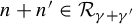 $n+n'\in \mathcal {R}_{\gamma +\gamma '}$
.
$n+n'\in \mathcal {R}_{\gamma +\gamma '}$
.
Lemma 5.3. If
 $0 < \gamma < \tfrac 12$
, then
$0 < \gamma < \tfrac 12$
, then
 $d(\mathcal {R}_{\gamma }+\mathcal {R}_{\gamma })=d(\mathcal {R}_{\gamma })=d(\mathcal {R})$
.
$d(\mathcal {R}_{\gamma }+\mathcal {R}_{\gamma })=d(\mathcal {R}_{\gamma })=d(\mathcal {R})$
.
Proof. Let
 $(N_k)_{k\geqslant 1}$
be an increasing sequence such that
$(N_k)_{k\geqslant 1}$
be an increasing sequence such that
 $$ \begin{align*}d_{(N_k)}(\mathcal{R}_{\gamma}) = \lim_{k \to \infty} \frac{|\mathcal{R}_{\gamma} \cap \{0,\ldots,N_k\}|}{N_k+1}\end{align*} $$
exists. By the mean ergodic theorem
 $$ \begin{align*} \nu(A) &\leqslant \lim_{k \to \infty} \frac{1}{N_k+1} \sum_{n=0}^{N_k} \frac{\nu(A \cap S^{-n}A)}{\nu(A)} = \lim_{k \to \infty} \frac{1}{N_k+1} \sum_{n=0}^{N_k} 1_{\mathcal{R}}(n) \frac{\nu(A \cap S^{-n}A)}{\nu(A)} \\ &\leqslant \lim_{k \to \infty} \frac{1}{N_k+1} \bigg( \sum_{n \in \mathcal{R}_{\gamma}, n \leqslant N_k} 1_{\mathcal{R}}(n) + \sum_{n \notin \mathcal{R}_{\gamma},n\leqslant N_k} 1_{\mathcal{R}}(n)(1-\gamma)\bigg) \\ &= d_{(N_k)}(\mathcal{R}_{\gamma}) + (1-\gamma)(d(\mathcal{R})-d_{(N_k)}(\mathcal{R}_{\gamma})). \end{align*} $$
Rearranging and using the assumption
 $d(\mathcal {R})=\nu (A)$
, it follows that
$d(\mathcal {R})=\nu (A)$
, it follows that
 $$ \begin{align*}\nu(A) \leqslant d_{(N_k)}(\mathcal{R}_{\gamma}) \leqslant d(\mathcal{R})=\nu(A).\end{align*} $$
Hence,
 $d_{(N_k)}(\mathcal {R}_{\gamma })=d(\mathcal {R})$
. By Lemma 5.2
$d_{(N_k)}(\mathcal {R}_{\gamma })=d(\mathcal {R})$
. By Lemma 5.2
 $\mathcal {R}_{\gamma }+\mathcal {R}_{\gamma } \subset \mathcal {R}_{2\gamma } \subset \mathcal {R}$
, so
$\mathcal {R}_{\gamma }+\mathcal {R}_{\gamma } \subset \mathcal {R}_{2\gamma } \subset \mathcal {R}$
, so
 $$ \begin{align*}d(\mathcal{R})=d_{(N_k)}(\mathcal{R}_{\gamma}) = \underline{d}_{(N_k)}(\mathcal{R}_{\gamma}) \leqslant \underline{d}_{(N_k)}(\mathcal{R}_{\gamma}+\mathcal{R}_{\gamma}) \leqslant \overline{d}_{(N_k)}(\mathcal{R}_{\gamma}+\mathcal{R}_{\gamma}) \leqslant d(\mathcal{R}).\end{align*} $$
Hence,
 $d_{(N_k)}(\mathcal {R}_{\gamma }+\mathcal {R}_{\gamma })$
exists and equals
$d_{(N_k)}(\mathcal {R}_{\gamma }+\mathcal {R}_{\gamma })$
exists and equals
 $d(\mathcal {R})$
. As
$d(\mathcal {R})$
. As
 $(N_k)_{k \geqslant 1}$
was arbitrary, the conclusion follows.
$(N_k)_{k \geqslant 1}$
was arbitrary, the conclusion follows.
For
 $0 < \gamma < \tfrac 12$
, Lemma 5.3 and Kneser’s theorem [Reference KneserKne53] (see also [Reference BiluBil97, Theorem 1.1]) therefore imply the existence of
$0 < \gamma < \tfrac 12$
, Lemma 5.3 and Kneser’s theorem [Reference KneserKne53] (see also [Reference BiluBil97, Theorem 1.1]) therefore imply the existence of
 $m \geqslant 1$
and
$m \geqslant 1$
and
 $K \subset \{0,\ldots ,m-1\}$
such that:
$K \subset \{0,\ldots ,m-1\}$
such that:
-
•
$\mathcal {R}_{\gamma } \subset K + m \mathbb {N}$
; -
•
$|K+K| = 2 |K| -1$
, where the operation on the left hand side is in
$ \mathbb {Z} /m \mathbb {Z}$
; and -
•
$\mathcal {R}_{\gamma } + \mathcal {R}_{\gamma } \subset K+K +m\mathbb {N}$
with
$ |(K+K +m\mathbb {N}) \setminus (\mathcal {R}_{\gamma } + \mathcal {R}_{\gamma })| < \infty $
.


It follows that
 $K = \{0\}$
, so
$K = \{0\}$
, so
 $\mathcal {R}_{\gamma } \subset m\mathbb {N}$
and
$\mathcal {R}_{\gamma } \subset m\mathbb {N}$
and
 $d(\mathcal {R})=d(\mathcal {R}_{\gamma })=d(\mathcal {R}_{\gamma }+\mathcal {R}_{\gamma })=m^{-1}$
. Further, for all
$d(\mathcal {R})=d(\mathcal {R}_{\gamma })=d(\mathcal {R}_{\gamma }+\mathcal {R}_{\gamma })=m^{-1}$
. Further, for all
 $n \in \mathcal {R}$
there exists
$n \in \mathcal {R}$
there exists
 $\gamma>0$
small enough such that
$\gamma>0$
small enough such that
 $n+\mathcal {R}_{\gamma } \subset \mathcal {R}$
by Lemma 5.2. As, in addition,
$n+\mathcal {R}_{\gamma } \subset \mathcal {R}$
by Lemma 5.2. As, in addition,
 $\mathcal {R}_{\gamma } \subset \mathcal {R}$
and
$\mathcal {R}_{\gamma } \subset \mathcal {R}$
and
 $d(\mathcal {R})=d(\mathcal {R}_{\gamma })$
, it follows that
$d(\mathcal {R})=d(\mathcal {R}_{\gamma })$
, it follows that
 $n \in m\mathbb {N}$
. Then the m sets
$n \in m\mathbb {N}$
. Then the m sets
 $S^{-i}A$
,
$S^{-i}A$
,
 $0\leqslant i \leqslant m-1$
are disjoint (up to
$0\leqslant i \leqslant m-1$
are disjoint (up to
 $\nu $
-null sets) and each of measure
$\nu $
-null sets) and each of measure
 $m^{-1}$
.
$m^{-1}$
.
Theorem 5.4. If
 $(X,\mathscr {B},\nu ,S)$
is ergodic and
$(X,\mathscr {B},\nu ,S)$
is ergodic and
 $$ \begin{align*}0< \underline{d}(\mathcal{R}) < \tfrac{3}{2} \nu(A),\end{align*} $$
then there exists an integer
 $m \geqslant 1$
such that
$m \geqslant 1$
such that
 $\mathcal {R} = m \mathbb {N}$
and
$\mathcal {R} = m \mathbb {N}$
and
 $X = \bigsqcup _{i=0}^{m-1} S^{-i} ( \bigcup _{j=0}^{\infty } S^{-jm}A )$
up to
$X = \bigsqcup _{i=0}^{m-1} S^{-i} ( \bigcup _{j=0}^{\infty } S^{-jm}A )$
up to
 $\nu $
-null sets.
$\nu $
-null sets.
Proof. By [Reference Björklund, Fish and ShkredovBFS21, §1.5] all the theorems in [Reference Björklund, Fish and ShkredovBFS21] hold for ergodic
 $\mathbb {N}$
-actions, so [Reference Björklund, Fish and ShkredovBFS21, Theorem 1.3] gives the existence of
$\mathbb {N}$
-actions, so [Reference Björklund, Fish and ShkredovBFS21, Theorem 1.3] gives the existence of
 $m \geqslant 1$
such that
$m \geqslant 1$
such that
 $\mathcal {R} = m \mathbb {N}$
. Therefore, the sets
$\mathcal {R} = m \mathbb {N}$
. Therefore, the sets
 $$ \begin{align*}\bigcup_{j=0}^{\infty} S^{-jm}A , S^{-1}\bigg(\bigcup_{j=0}^{\infty} S^{-jm}A\bigg) ,\ldots,S^{-(m-1)}\bigg(\bigcup_{j=0}^{\infty} S^{-jm}A \bigg)\end{align*} $$
are mutually disjoint up to
 $\nu $
-null sets, and ergodicity implies that they partition X.
$\nu $
-null sets, and ergodicity implies that they partition X.
6 Inverse theorems for trees
In this section, we prove inverse results for Theorems 4.1 and 4.2 (Theorems 6.1, 6.2 and 6.4) using the results of the previous section.
Theorem 6.1. If T is a tree and
 $2 \leqslant r \leqslant q$
with
$2 \leqslant r \leqslant q$
with
 $$ \begin{align*}\overline{d}(\overline{G}(F^r)) =\frac{\overline{\dim}_MT - \log_q(r-1)}{1-\log_q(r-1)}>0,\end{align*} $$
then
 $\overline {\dim }_M T = m^{-1}(1-\log _q(r-1))+\log _q(r-1)$
for some positive integer m. Moreover,
$\overline {\dim }_M T = m^{-1}(1-\log _q(r-1))+\log _q(r-1)$
for some positive integer m. Moreover,
 $\overline {d}(V_1^{r,m,mk})>0$
for every
$\overline {d}(V_1^{r,m,mk})>0$
for every
 $k \geqslant 1$
.
$k \geqslant 1$
.
Proof. Let
 $\mathcal {R} = \{n \in \mathbb {N} \colon \widetilde {\mu }(A_r \cap S^{-n}A_r)>0\}$
. Combining the proof of Theorem 4.1 and the hypothesis, we obtain
$\mathcal {R} = \{n \in \mathbb {N} \colon \widetilde {\mu }(A_r \cap S^{-n}A_r)>0\}$
. Combining the proof of Theorem 4.1 and the hypothesis, we obtain
 $$ \begin{align*}\overline{d}(\overline{G}(F^r)) \geqslant \overline{d}(\mathcal{R}) \geqslant \underline{d}(\mathcal{R}) \geqslant \widetilde{\mu}(A_r) \geqslant \frac{\overline{\dim}_MT - \log_q(r-1)}{1-\log_q(r-1)}=\overline{d}(\overline{G}(F^r)).\end{align*} $$
Therefore,
 $\widetilde {\mu }(A_r) = \overline {d}(\overline {G}(F^r)) = \overline {d}(\mathcal {R})=\underline {d}(\mathcal {R})$
is positive; by Theorem 5.1 it equals
$\widetilde {\mu }(A_r) = \overline {d}(\overline {G}(F^r)) = \overline {d}(\mathcal {R})=\underline {d}(\mathcal {R})$
is positive; by Theorem 5.1 it equals
 $m^{-1}$
for some positive integer m, and
$m^{-1}$
for some positive integer m, and
 $\widetilde {M} =\bigsqcup _{i=0}^{m-1} S^{-i} A_r$
up to
$\widetilde {M} =\bigsqcup _{i=0}^{m-1} S^{-i} A_r$
up to
 $\widetilde {\mu }$
-null sets.
$\widetilde {\mu }$
-null sets.
The above also shows that equality holds in Proposition 2.7 for
 $\widetilde {\mu }$
, whence
$\widetilde {\mu }$
, whence
 $\int _{A_r} H\,d\widetilde {\mu } = \widetilde {\mu }(A_r)$
and
$\int _{A_r} H\,d\widetilde {\mu } = \widetilde {\mu }(A_r)$
and
 $\int _{A_r^c}H\,d\widetilde {\mu } = (1-\widetilde {\mu }(A_r))\log _q(r-1)$
. The bounds on H then imply
$\int _{A_r^c}H\,d\widetilde {\mu } = (1-\widetilde {\mu }(A_r))\log _q(r-1)$
. The bounds on H then imply
 $\widetilde {\mu }$
-almost everywhere equalities
$\widetilde {\mu }$
-almost everywhere equalities
 $$ \begin{align} \prod_{i \in \Lambda} P1_{B_i}=c_11_{A_r}=c_11_{A_q}, \end{align} $$
 $$ \begin{align} 1_{A_{r-1}}\sum_{\substack{I \subset \Lambda \\ |I|=r-1}} \prod_{i \in I} P1_{B_i} = 1_{A_r^c}\sum_{\substack{I \subset \Lambda \\ |I|=r-1}} \prod_{i \in I} P1_{B_i} = c_21_{A_r^c}, \end{align} $$
where
 $c_1 = q^{-q}$
and
$c_1 = q^{-q}$
and
 $c_2 = (r-1)^{1-r}$
.
$c_2 = (r-1)^{1-r}$
.
Recall from §3.1 the operators
 $R_{r-1,1}$
and
$R_{r-1,1}$
and
 $R_{q,1}$
on
$R_{q,1}$
on
 $L^{\infty }(\widetilde {M},\widetilde {\mu })$
, which, for simplicity, we denote by
$L^{\infty }(\widetilde {M},\widetilde {\mu })$
, which, for simplicity, we denote by
 $R_1$
and
$R_1$
and
 $R_2$
:
$R_2$
:
 $$ \begin{align*}R_1f = \sum_{\substack{I \subset \Lambda \\ |I|=r-1}} \prod_{i \in I} P(1_{B_i}f); \quad R_2f = \prod_{i \in \Lambda} P(1_{B_i}f).\end{align*} $$
Using the facts determined previously, we compute
 $\phi _{V_1^{r,m,mk}}' =(R_2R_1^{m-1})^k1_{A_q}$
. In the following, equalities are only up to
$\phi _{V_1^{r,m,mk}}' =(R_2R_1^{m-1})^k1_{A_q}$
. In the following, equalities are only up to
 $\widetilde {\mu }$
-null sets. We compute first the case
$\widetilde {\mu }$
-null sets. We compute first the case
 $k=1$
. Note that
$k=1$
. Note that
 $A_q = S^{-m}A_q$
and
$A_q = S^{-m}A_q$
and
 $1_{S^{-i}A_q} = S1_{S^{-i+1}A_q}$
for
$1_{S^{-i}A_q} = S1_{S^{-i+1}A_q}$
for
 $i \geqslant 1$
. By Lemma 2.8
$i \geqslant 1$
. By Lemma 2.8
 $$ \begin{align*} R_11_{A_q} = \sum_{\substack{I \subset \Lambda \\ |I|=r-1}} \prod_{i \in I} P(1_{B_i}1_{A_q}) &= \sum_{\substack{I \subset \Lambda \\ |I|=r-1}}\prod_{i \in I} P(1_{B_i}S1_{S^{-m+1}A_q}) \\ &= 1_{S^{-m+1}A_q}\sum_{\substack{I \subset \Lambda \\ |I|=r-1}} \prod_{i \in I} P1_{B_i} \\ &= c_21_{S^{-m+1}A_q}, \end{align*} $$
where the last equality follows from (10) and the fact
 $S^{-m+1}A_q =S^{-m+1}A_r \subset A_r^c$
. As
$S^{-m+1}A_q =S^{-m+1}A_r \subset A_r^c$
. As
 $R_1$
is homogeneous of degree
$R_1$
is homogeneous of degree
 $r-1$
, repeating this calculation gives
$r-1$
, repeating this calculation gives
 $$ \begin{align*}R_1^{m-1}1_{A_q}=c_2^{\sum_{j=0}^{m-2}(r-1)^j}1_{S^{-1}A_q}\end{align*} $$
and, hence,
 $$ \begin{align*} \phi_{V_1^{r,m,m}}' &= R_2\bigg(c_2^{\sum_{j=0}^{m-2}(r-1)^j}1_{S^{-1}A_q}\bigg) \\ &= c_2^{q\sum_{j=0}^{m-2}(r-1)^j}\prod_{i \in \Lambda}P(1_{B_i}S1_{A_q}) \\ &= c_2^{q\sum_{j=0}^{m-2}(r-1)^j}1_{A_q}\prod_{i \in \Lambda} P1_{B_i} \\ &= c_1c_2^{q\sum_{j=0}^{m-2}(r-1)^j}1_{A_q}. \end{align*} $$
Letting
 $d_1 = c_1c_2^{q\sum _{j=0}^{m-2}(r-1)^j}$
and defining inductively
$d_1 = c_1c_2^{q\sum _{j=0}^{m-2}(r-1)^j}$
and defining inductively
 $d_k = d_{k-1}^{q(r-1)^{m-1}}d_1$
, it follows that
$d_k = d_{k-1}^{q(r-1)^{m-1}}d_1$
, it follows that
 $\phi _{V_1^{r,m,mk}}' = d_k1_{A_q} \ \widetilde {\mu }$
-almost everywhere. Then
$\phi _{V_1^{r,m,mk}}' = d_k1_{A_q} \ \widetilde {\mu }$
-almost everywhere. Then
 $$ \begin{align*}\overline{d}(V_1^{r,m,mk}) \geqslant \int_{\widetilde{M}} \phi_{V_1^{r,m,mk}}\,d\widetilde{\mu} \geqslant \int_{\widetilde{M}} \phi_{V_1^{r,m,mk}}'\,d\widetilde{\mu} = d_k\widetilde{\mu}(A_q) = \frac{d_k}{m}>0\end{align*} $$
for all
 $k \geqslant 1$
by the correspondence principle Theorem 3.4.
$k \geqslant 1$
by the correspondence principle Theorem 3.4.
Theorem 6.2. If T is a tree and
 $2 \leqslant r \leqslant q$
with
$2 \leqslant r \leqslant q$
with
 $$ \begin{align} \underline{d}(G^{\ast}(F^r)) =\frac{\dim T - \log_q(r-1)}{1-\log_q(r-1)}>0 \end{align} $$
or
 $$ \begin{align} \overline{d}(G^{\ast}(D^{r,2})) =\frac{\dim T - \log_q(r-1)}{1-\log_q(r-1)}>0, \end{align} $$
then
 $\dim T = m^{-1}(1-\log _q(r-1))+\log _q(r-1)$
for some positive integer m. Moreover,
$\dim T = m^{-1}(1-\log _q(r-1))+\log _q(r-1)$
for some positive integer m. Moreover,
 $d^{\ast }(V_1^{r,m,mk})>0$
for every
$d^{\ast }(V_1^{r,m,mk})>0$
for every
 $k \geqslant 1$
.
$k \geqslant 1$
.
Proof. Fix
 $\epsilon>0$
small enough, and let
$\epsilon>0$
small enough, and let
 $\mathcal {R} = \{n \in \mathbb {N} \colon \widetilde {\eta _{\epsilon }}(A_r \cap S^{-n}A_r)>0\}$
. In the case of (11), from the proof of Theorem 4.1 we have
$\mathcal {R} = \{n \in \mathbb {N} \colon \widetilde {\eta _{\epsilon }}(A_r \cap S^{-n}A_r)>0\}$
. In the case of (11), from the proof of Theorem 4.1 we have
 $$ \begin{align*} \frac{\dim T - \log_q(r-1)}{1-\log_q(r-1)} = \underline{d}(G^{\ast}(F^r)) \geqslant \underline{d}(\mathcal{R}) \geqslant \widetilde{\eta_{\epsilon}}(A_r) \geqslant \frac{\dim T - \epsilon -\log_q(r-1)}{1-\log_q(r-1)}, \end{align*} $$
so
 $\underline {d}(\mathcal {R}) \leqslant \tfrac 32\widetilde {\eta _{\epsilon }}(A_r)$
for small enough
$\underline {d}(\mathcal {R}) \leqslant \tfrac 32\widetilde {\eta _{\epsilon }}(A_r)$
for small enough
 $\epsilon $
. By Theorem 5.4 there is a positive integer m such that
$\epsilon $
. By Theorem 5.4 there is a positive integer m such that
 $\mathcal {R}=m\mathbb {N}$
and
$\mathcal {R}=m\mathbb {N}$
and
 $\widetilde {M} =\bigsqcup _{i=0}^{m-1} S^{-i} ( \bigcup _{j=0}^{\infty } S^{-mj}A_r ) $
up to
$\widetilde {M} =\bigsqcup _{i=0}^{m-1} S^{-i} ( \bigcup _{j=0}^{\infty } S^{-mj}A_r ) $
up to
 $\widetilde {\eta _{\epsilon }}$
-null sets.
$\widetilde {\eta _{\epsilon }}$
-null sets.
In the case of (12), we invoke the proof of Theorem 4.2. Recall that there exist a measurable set Z such that
 $A_r \subset Z$
modulo
$A_r \subset Z$
modulo
 $\widetilde {\eta _{\epsilon }}$
-null sets and an increasing chain of measurable sets
$\widetilde {\eta _{\epsilon }}$
-null sets and an increasing chain of measurable sets
 $(Z_{\rho })_{\rho>0}$
with
$(Z_{\rho })_{\rho>0}$
with
 $\bigcup _{\rho> 0} Z_{\rho } = Z$
such that for every
$\bigcup _{\rho> 0} Z_{\rho } = Z$
such that for every
 $\delta> 0$
we have
$\delta> 0$
we have
 $$ \begin{align*} \frac{\dim T - \log_q(r-1)}{1-\log_q(r-1)} &= \overline{d}(G^{\ast}(D^{r,2})) \geqslant \overline{d}(\mathcal{R}^{\delta}(Z_{\rho})) \\ &\geqslant \bigg( \liminf_{N \to \infty} \frac{1}{N+1} \sum_{n=0}^N \frac{\widetilde{\eta_{\epsilon}}(Z_{\rho} \cap S^{-n}Z_{\rho})}{\widetilde{\eta_{\epsilon}}(Z_{\rho})} \bigg) - \delta\widetilde{\eta_{\epsilon}}(Z_{\rho}) \\ &\geqslant (1-\delta)\widetilde{\eta_{\epsilon}}(Z_{\rho}) \xrightarrow{\delta \to 0} \widetilde{\eta_{\epsilon}}(Z_{\rho}) \xrightarrow{\rho \to 0} \widetilde{\eta_{\epsilon}}(Z) \\ &\geqslant \widetilde{\eta_{\epsilon}}(A_r) \geqslant \frac{\dim T - \epsilon-\log_q(r-1)}{1-\log_q(r-1)}, \end{align*} $$
where
 $\mathcal {R}^{\delta }(Z_{\rho }) = \{ n \in \mathbb {N} \colon \widetilde {\eta _{\epsilon }}(Z_{\rho } \cap S^{-n}Z_{\rho })> \delta \widetilde {\eta _{\epsilon }}(Z_{\rho })^2\}$
. Hence, for small enough
$\mathcal {R}^{\delta }(Z_{\rho }) = \{ n \in \mathbb {N} \colon \widetilde {\eta _{\epsilon }}(Z_{\rho } \cap S^{-n}Z_{\rho })> \delta \widetilde {\eta _{\epsilon }}(Z_{\rho })^2\}$
. Hence, for small enough
 $\epsilon $
and
$\epsilon $
and
 $\rho $
the assumptions of Theorem A.3 are satisfied, so there exists
$\rho $
the assumptions of Theorem A.3 are satisfied, so there exists
 $m \geqslant 1$
such that
$m \geqslant 1$
such that
 $\mathcal {R}(Z_{\rho }) = \mathcal {R}^{\delta }(Z_{\rho }) = m \mathbb {N}$
, where
$\mathcal {R}(Z_{\rho }) = \mathcal {R}^{\delta }(Z_{\rho }) = m \mathbb {N}$
, where
 $\mathcal {R}(Z_{\rho }) = \{ n \in \mathbb {N} \colon \widetilde {\eta _{\epsilon }}(Z_{\rho } \cap S^{-n}Z_{\rho })> 0 \}$
. As this is true for all
$\mathcal {R}(Z_{\rho }) = \{ n \in \mathbb {N} \colon \widetilde {\eta _{\epsilon }}(Z_{\rho } \cap S^{-n}Z_{\rho })> 0 \}$
. As this is true for all
 $\rho> 0$
small enough and
$\rho> 0$
small enough and
 $\mathcal {R} \subset \bigcup _{\rho> 0} \mathcal {R}(Z_{\rho })$
, we conclude that for
$\mathcal {R} \subset \bigcup _{\rho> 0} \mathcal {R}(Z_{\rho })$
, we conclude that for
 $\epsilon $
small enough there exists
$\epsilon $
small enough there exists
 $m \geqslant 1$
such that
$m \geqslant 1$
such that
 $\mathcal {R} \subset m \mathbb {N}$
. This immediately implies that
$\mathcal {R} \subset m \mathbb {N}$
. This immediately implies that
 ${\widetilde {M} =\bigsqcup _{i=0}^{m-1} S^{-i} ( \bigcup _{j=0}^{\infty } S^{-mj}A_r ) }$
up to
${\widetilde {M} =\bigsqcup _{i=0}^{m-1} S^{-i} ( \bigcup _{j=0}^{\infty } S^{-mj}A_r ) }$
up to
 $\widetilde {\eta _{\epsilon }}$
-null sets.
$\widetilde {\eta _{\epsilon }}$
-null sets.
In both cases, for small
 $\epsilon $
the above inequalities force
$\epsilon $
the above inequalities force
 $$ \begin{align*}\frac{\dim T - \log_q(r-1)}{1-\log_q(r-1)} = m^{-1},\end{align*} $$
and, hence,
 $$ \begin{align} \widetilde{\eta_{\epsilon}}(A_r) \geqslant (1 - \epsilon') m^{-1} = (1- \epsilon') \widetilde{\eta_{\epsilon}}\bigg(\bigcup_{j=0}^{\infty} S^{-mj}A_r\bigg), \end{align} $$
where
 $\epsilon ' \to 0$
as
$\epsilon ' \to 0$
as
 $\epsilon \to 0$
. We also have
$\epsilon \to 0$
. We also have
 $$ \begin{align*}\dim T \geqslant \widetilde{\eta_{\epsilon}}(A_r)+(1-\widetilde{\eta_{\epsilon}}(A_r))\log_q(r-1) \geqslant H(\widetilde{\eta_{\epsilon}}) \geqslant \dim T-\epsilon\end{align*} $$
and, hence, the pair of inequalities
 $$ \begin{align} \phantom{\hspace{-27pt}}\int_{A_r} H\,d\widetilde{\eta_{\epsilon}}&\geqslant \widetilde{\eta_{\epsilon}}(A_r)-\epsilon,\qquad\quad\qquad \end{align} $$
 $$ \begin{align} \int_{A_r^c} H\,d\widetilde{\eta_{\epsilon}} &\geqslant (1-\widetilde{\eta_{\epsilon}}(A_r))\log_q(r-1)-\epsilon. \end{align} $$
We denote by
 $\mathbf {A}_{\mathbf {r}} = \bigcup _{j=0}^{\infty } S^{-mj}A_r$
. Then we have
$\mathbf {A}_{\mathbf {r}} = \bigcup _{j=0}^{\infty } S^{-mj}A_r$
. Then we have
 $\widetilde {M} = \bigsqcup _{i=0}^{m-1} S^{-i}\mathbf {A}_{\mathbf {r}}$
. Given
$\widetilde {M} = \bigsqcup _{i=0}^{m-1} S^{-i}\mathbf {A}_{\mathbf {r}}$
. Given
 $\widetilde {\tau } \in \widetilde {M}$
and
$\widetilde {\tau } \in \widetilde {M}$
and
 $E \subset \widetilde {M}$
, observe that
$E \subset \widetilde {M}$
, observe that
 $S^{-i}(\widetilde {\tau }) \subset E$
if and only if
$S^{-i}(\widetilde {\tau }) \subset E$
if and only if
 $P^i1_E(\widetilde {\tau }) = 1$
. For
$P^i1_E(\widetilde {\tau }) = 1$
. For
 $i \geqslant 0$
, define
$i \geqslant 0$
, define
 $E_i$
to be
$E_i$
to be
 $\mathbf {A}_{\mathbf {r}}$
if m divides i and
$\mathbf {A}_{\mathbf {r}}$
if m divides i and
 $\mathbf {A}_{\mathbf {r}}^{\mathbf {c}}$
otherwise. Then the m-periodicity of
$\mathbf {A}_{\mathbf {r}}^{\mathbf {c}}$
otherwise. Then the m-periodicity of
 $\mathbf {A}_{\mathbf {r}}$
and
$\mathbf {A}_{\mathbf {r}}$
and
 $\mathbf {A}_{\mathbf {r}}^{\mathbf {c}} =\bigsqcup _{i=1}^{m-1} S^{-i} \mathbf {A}_{\mathbf {r}}$
under
$\mathbf {A}_{\mathbf {r}}^{\mathbf {c}} =\bigsqcup _{i=1}^{m-1} S^{-i} \mathbf {A}_{\mathbf {r}}$
under
 $S^{-1}$
gives
$S^{-1}$
gives
 $\widetilde {\eta _{\epsilon }}$
-almost everywhere equalities
$\widetilde {\eta _{\epsilon }}$
-almost everywhere equalities
 $$ \begin{align*}P^i1_{E_i} = P^iS^i1_{S^{-i}E_i} = 1_{S^{-i}E_i},\end{align*} $$
so the set
 $\mathbf {A}_{\mathbf {r'}} = \bigcap _{i \geqslant 0} \{ \widetilde {\tau } \in \widetilde {M} \colon P^i1_{E_i}(\widetilde {\tau }) = 1\}$
is a
$\mathbf {A}_{\mathbf {r'}} = \bigcap _{i \geqslant 0} \{ \widetilde {\tau } \in \widetilde {M} \colon P^i1_{E_i}(\widetilde {\tau }) = 1\}$
is a
 $\widetilde {\eta _{\epsilon }}$
-conull subset of
$\widetilde {\eta _{\epsilon }}$
-conull subset of
 $\mathbf {A}_{\mathbf {r}}$
.
$\mathbf {A}_{\mathbf {r}}$
.
Define for
 $\delta>0$
the set
$\delta>0$
the set
 $$ \begin{align*}A_\delta = \bigcap_{i=0}^{mk} \{ \widetilde{\tau} \in \mathbf{A}_{\mathbf{r'}} \colon P^iH(\widetilde{\tau}) \geqslant c_i-\delta\}, \quad c_i = \begin{cases} 1, & m \mid i,\\ \log_{q}(r-1) & \text{otherwise}. \end{cases} \end{align*} $$
It follows from (13) and inequalities (14) and (15) that by choosing
 $\epsilon $
small enough we can guarantee that
$\epsilon $
small enough we can guarantee that
 $\widetilde {\eta _{\epsilon }}(A_\delta )> 0$
. We show the existence of
$\widetilde {\eta _{\epsilon }}(A_\delta )> 0$
. We show the existence of
 $\delta $
such that the configuration
$\delta $
such that the configuration
 $V_1^{r,m,mk}$
appears at the root of
$V_1^{r,m,mk}$
appears at the root of
 $|\tau _0|$
for every
$|\tau _0|$
for every
 $\widetilde {\tau } = (\tau _i)_{i \leqslant 0} \in A_\delta $
. First note that, by the construction of
$\widetilde {\tau } = (\tau _i)_{i \leqslant 0} \in A_\delta $
. First note that, by the construction of
 $\mathbf {A}_{\mathbf {r'}}$
, if
$\mathbf {A}_{\mathbf {r'}}$
, if
 $\widetilde {\tau } \in A_\delta $
and
$\widetilde {\tau } \in A_\delta $
and
 $v \in |\tau _0|$
with
$v \in |\tau _0|$
with
 $0 \leqslant l(v) \leqslant mk$
, then
$0 \leqslant l(v) \leqslant mk$
, then
 $H(\widetilde {\tau }^v) \leqslant c_{l(v)}$
. Hence, for
$H(\widetilde {\tau }^v) \leqslant c_{l(v)}$
. Hence, for
 ${0 \leqslant i \leqslant mk}$
 $$ \begin{align} c_i-\delta \leqslant P^iH(\widetilde{\tau}) = \sum_{l(v) = i} \tau_0(v)H(\widetilde{\tau}^v) \leqslant c_i. \end{align} $$
If
 $H(\widetilde {\tau })> \log _q(q-1)$
, then
$H(\widetilde {\tau })> \log _q(q-1)$
, then
 $\widetilde {\tau } \in A_q$
, and if
$\widetilde {\tau } \in A_q$
, and if
 $H(\widetilde {\tau })> \log _q(r-2)$
, then
$H(\widetilde {\tau })> \log _q(r-2)$
, then
 $\widetilde {\tau } \in A_{r-1}$
. To prove the appearance of
$\widetilde {\tau } \in A_{r-1}$
. To prove the appearance of
 $V_1^{r,m,mk}$
at the root of
$V_1^{r,m,mk}$
at the root of
 $|\tau _0|$
it therefore suffices to give sufficiently large lower bounds for
$|\tau _0|$
it therefore suffices to give sufficiently large lower bounds for
 $H(\widetilde {\tau }^v)$
for
$H(\widetilde {\tau }^v)$
for
 $l(v) \leqslant mk$
.
$l(v) \leqslant mk$
.
Lemma 6.3. For every
 $\delta _1,\delta _2>0$
there exists
$\delta _1,\delta _2>0$
there exists
 $\delta>0$
such that for
$\delta>0$
such that for
 $1 \leqslant j \leqslant mk+1$
: (a) the set
$1 \leqslant j \leqslant mk+1$
: (a) the set
 $\{\tau _0(v) \colon \widetilde {\tau } \in A_\delta , v \in |\tau _0|(j)\} \subset [0,1]$
is contained in an interval of length less than
$\{\tau _0(v) \colon \widetilde {\tau } \in A_\delta , v \in |\tau _0|(j)\} \subset [0,1]$
is contained in an interval of length less than
 $\delta _1$
; and (b) for all
$\delta _1$
; and (b) for all
 $\widetilde {\tau } \in A_\delta $
and
$\widetilde {\tau } \in A_\delta $
and
 $v \in |\tau _0|$
with
$v \in |\tau _0|$
with
 $l(v) \leqslant j-1$
we have
$l(v) \leqslant j-1$
we have
 $H(\widetilde {\tau }^v) \geqslant c_{l(v)}-\delta _2$
.
$H(\widetilde {\tau }^v) \geqslant c_{l(v)}-\delta _2$
.
Proof. We prove both statements simultaneously by induction on j. For
 $j=1$
we have
$j=1$
we have
 $H(\widetilde {\tau }) \geqslant 1-\delta $
for all
$H(\widetilde {\tau }) \geqslant 1-\delta $
for all
 $\widetilde {\tau } \in A_\delta $
by (16), so any
$\widetilde {\tau } \in A_\delta $
by (16), so any
 $\delta < \delta _2$
suffices. Further, observe that H is a continuous function attaining its maximum at
$\delta < \delta _2$
suffices. Further, observe that H is a continuous function attaining its maximum at
 $\widetilde {\tau }$
such that
$\widetilde {\tau }$
such that
 $p_{\widetilde {\tau }}(B_i) =q^{-1}$
for all
$p_{\widetilde {\tau }}(B_i) =q^{-1}$
for all
 $i \in \Lambda $
. Hence, given
$i \in \Lambda $
. Hence, given
 $\delta _1>0$
, the set
$\delta _1>0$
, the set
 $\{\tau _0(v) \colon \widetilde {\tau } \in A_\delta , v \in |\tau _0|(1)\}$
is contained in an interval of length
$\{\tau _0(v) \colon \widetilde {\tau } \in A_\delta , v \in |\tau _0|(1)\}$
is contained in an interval of length
 $<\delta _1$
(containing
$<\delta _1$
(containing
 $q^{-1}$
) for
$q^{-1}$
) for
 $\delta $
small enough.
$\delta $
small enough.
Assuming the lemma is true for
 $j \leqslant i < mk+1$
, we prove it for
$j \leqslant i < mk+1$
, we prove it for
 $j=i+1$
. We first consider statement (b). For
$j=i+1$
. We first consider statement (b). For
 $w \in |\tau _0|(i)$
with
$w \in |\tau _0|(i)$
with
 $\widetilde {\tau } \in A_\delta $
the inequality (16) gives
$\widetilde {\tau } \in A_\delta $
the inequality (16) gives
 $$ \begin{align*}c_i - \delta \leqslant P^iH(\widetilde{\tau}) = \sum_{l(v)=i} \tau_0(v)H(\widetilde{\tau}^v) \leqslant \tau_0(w)H(\widetilde{\tau}^w) + (1-\tau_0(w)) c_i,\end{align*} $$
and rearranging gives
 $$ \begin{align*}c_i - \frac{\delta}{\tau_0(w)} \leqslant H(\widetilde{\tau}^w). \end{align*} $$
By statement (a) of the induction hypothesis,
 $$ \begin{align*}\sup_{\widetilde{\tau} \in A_\delta, w \in |\tau_0|(i)} \frac{\delta}{\tau_0(w)} \to 0\end{align*} $$
as
 $\delta \to 0$
, so by taking
$\delta \to 0$
, so by taking
 $\delta $
small enough, statement (b) is satisfied for
$\delta $
small enough, statement (b) is satisfied for
 $j=i+1$
. Combining statement (a) for
$j=i+1$
. Combining statement (a) for
 $j=i$
and statement (b) for
$j=i$
and statement (b) for
 $j=i+1$
with the same argument as in the base case proves statement (a), noting that if m does not divide j, then we consider maxima of H on
$j=i+1$
with the same argument as in the base case proves statement (a), noting that if m does not divide j, then we consider maxima of H on
 $A_r^c$
.
$A_r^c$
.
It follows that any
 $V_1^{r,m,mk}$
-detecting function is positive on
$V_1^{r,m,mk}$
-detecting function is positive on
 $A_\delta $
. By the correspondence principle Theorem 3.5 we have for all
$A_\delta $
. By the correspondence principle Theorem 3.5 we have for all
 $\epsilon>0$
 $$ \begin{align*}d^{\ast}(V_1^{r,m,mk}) \geqslant \int_{\widetilde{M}} \phi_{V_1^{r,m,mk}}\,d\widetilde{\eta_{\epsilon}} \geqslant \int_{A_\delta} \phi_{V_1^{r,m,mk}}\,d\widetilde{\eta_{\epsilon}}>0,\end{align*} $$
because
 $\widetilde {\eta _{\epsilon }}(A_\delta )>0$
.
$\widetilde {\eta _{\epsilon }}(A_\delta )>0$
.
Theorem 6.4. Let
 $\beta \kern1.2pt{<}\kern1.2pt 3/2$
and assume that
$\beta \kern1.2pt{<}\kern1.2pt 3/2$
and assume that
 $$ \begin{align*} 0 < \underline {d}(G^{\ast }(F^r)) < \beta \cdot \frac{({\dim T - \log _q(r - 1)})}{({1-\log _q(r-1)})}. \end{align*} $$
Then there exists an integer
 $m \geqslant 1$
such that
$m \geqslant 1$
such that
 $m \mathbb {N} \subset G^{\ast }(F^r)$
.
$m \mathbb {N} \subset G^{\ast }(F^r)$
.
Proof. For small enough
 $\epsilon>0$
, by the correspondence principle Theorem 3.5 and the proof of Theorem 4.1
$\epsilon>0$
, by the correspondence principle Theorem 3.5 and the proof of Theorem 4.1
 $$ \begin{align*} \beta\widetilde{\eta_{\epsilon}}(A_r) \geqslant \beta \frac{\dim T-\epsilon-\log_q(r-1)}{1-\log_q(r-1)}>\underline{d}(G^{\ast}(F^r)) \geqslant \underline{d}(\mathcal{R}), \end{align*} $$
where
 $\mathcal {R} = \{ n \in \mathbb {N} \colon \widetilde {\eta _{\epsilon }}(A_r \cap S^{-n} A_r)> 0 \}$
. Theorem 5.4 then implies that there exists
$\mathcal {R} = \{ n \in \mathbb {N} \colon \widetilde {\eta _{\epsilon }}(A_r \cap S^{-n} A_r)> 0 \}$
. Theorem 5.4 then implies that there exists
 $m \geqslant 1$
such that
$m \geqslant 1$
such that
 $m\mathbb {N} = \mathcal {R} \subset G^{\ast }(F^r)$
.
$m\mathbb {N} = \mathcal {R} \subset G^{\ast }(F^r)$
.
Question 6.5. It follows from the work of Furstenberg and Weiss in [Reference Furstenberg and WeissFW03] that for every k there exists n such that
 $d^{\ast }(D^{2,k}_n)>0$
provided that
$d^{\ast }(D^{2,k}_n)>0$
provided that
 $\dim T>0$
. On the other hand, under the assumptions of Theorem 6.4, there exists
$\dim T>0$
. On the other hand, under the assumptions of Theorem 6.4, there exists
 $m\geqslant 1$
such that
$m\geqslant 1$
such that
 $m \mathbb {N} \subset G^{\ast }(F)$
. In analogy to Proposition 1.5, is it true that the stronger claim
$m \mathbb {N} \subset G^{\ast }(F)$
. In analogy to Proposition 1.5, is it true that the stronger claim
 $d^{\ast }(D^{2,k}_m)> 0$
holds true for every k satisfying
$d^{\ast }(D^{2,k}_m)> 0$
holds true for every k satisfying
 $(1-\beta ^{-1})k < 1$
?
$(1-\beta ^{-1})k < 1$
?
Acknowledgements
We thank Michael Björklund and James Parkinson. The current paper is a sequel of joint works of A.F. and I.S. with them. A.F. is grateful to Itai Benjamini for inspiring conversations on the subject during his visit to the Weizmann Institute hosted by Omri Sarig. He thanks Omri and the Weizmann Institute for hospitality. He also thanks Haotian Wu and Cecilia González Tokman for fruitful discussions. I.S. is grateful to SMRI and the School of Mathematics and Statistics at the University of Sydney for funding his visit and for their hospitality. We also thank the anonymous referee for a thorough reading of the paper, which led to many improvements.
A Appendix. Stability in an inverse theorem for return times of ergodic systems
In the proof of Theorem 6.2 for the configuration
 $D^{r,2}$
, we are unable to apply Theorem 5.4 because we have no upper bound for
$D^{r,2}$
, we are unable to apply Theorem 5.4 because we have no upper bound for
 $\underline {d}(\mathcal {R})$
. However, we have bounds on the densities of the sets of
$\underline {d}(\mathcal {R})$
. However, we have bounds on the densities of the sets of
 $\delta $
-return times. Here we prove a stability result (Theorem A.3) giving the same conclusion as Theorem 5.4 under assumptions involving
$\delta $
-return times. Here we prove a stability result (Theorem A.3) giving the same conclusion as Theorem 5.4 under assumptions involving
 $\delta $
-return times instead of return times.
$\delta $
-return times instead of return times.
Given an ergodic measure-preserving system
 $(X,\mathscr {B},\nu ,S)$
and
$(X,\mathscr {B},\nu ,S)$
and
 $A \in \mathscr {B}$
with
$A \in \mathscr {B}$
with
 $\nu (A)>0$
, define for
$\nu (A)>0$
, define for
 $\delta>0$
the set of
$\delta>0$
the set of
 $\delta $
-return times of A
$\delta $
-return times of A
 $$ \begin{align*} \mathcal{R}^{\delta} = \{ n \in \mathbb{N} \colon \nu(A \cap S^{-n}A)> \delta \nu(A)^2 \}. \end{align*} $$
Define also for
 $0<\gamma <1$
the set
$0<\gamma <1$
the set
 $$ \begin{align*}\mathcal{R}_{\gamma} = \{n \in \mathbb{N} \colon \nu(A \cap S^{-n}A) \geqslant (1-\gamma)\nu(A)\}.\end{align*} $$
Lemma A.1. If
 $\overline {d}(\mathcal {R}^{\delta }) \leqslant (1+\eta )\nu (A)$
for all
$\overline {d}(\mathcal {R}^{\delta }) \leqslant (1+\eta )\nu (A)$
for all
 $\delta>0$
, then for any
$\delta>0$
, then for any
 $\gamma>0$
 $$ \begin{align*}\underline{d}(\mathcal{R}_{\gamma}) \geqslant \bigg(\frac{\gamma-\eta+\gamma\eta}{\gamma}\bigg)\nu(A).\end{align*} $$
Proof. Given
 $\gamma $
, choose
$\gamma $
, choose
 $\delta $
such that
$\delta $
such that
 $0 < \delta < ({1-\gamma })/{\nu (A)}$
(so
$0 < \delta < ({1-\gamma })/{\nu (A)}$
(so
 $\mathcal {R}_{\gamma } \subset \mathcal {R}^{\delta }$
). First, observe that by the mean ergodic theorem,
$\mathcal {R}_{\gamma } \subset \mathcal {R}^{\delta }$
). First, observe that by the mean ergodic theorem,
 $$ \begin{align} \underline{d}(\mathcal{R}^{\delta}) &= \liminf_{N \to \infty} \frac{1}{N+1} \sum_{n=0}^N 1_{\mathcal{R}^{\delta}}(n)\nonumber\\[4pt] &\geqslant \liminf_{N \to \infty} \frac{1}{N+1} \sum_{n=0}^N \frac{\nu(A \cap S^{-n}A)}{\nu(A)}-\delta\nu(A) = (1-\delta)\nu(A). \end{align} $$
Let
 $(N_k)_{k \geqslant 1}$
be an increasing sequence such that
$(N_k)_{k \geqslant 1}$
be an increasing sequence such that
 $$ \begin{align*} \underline {d}(\mathcal {R}_{\gamma }) = \lim _{k \to \infty } (N_k+1)^{-1} \sum _{n=0}^{N_k} 1_{\mathcal {R}_{\gamma }}(n). \end{align*} $$
By the mean ergodic theorem
 $$ \begin{align*} \nu(A) &= \lim_{k \to \infty} \frac{1}{N_k+1} \sum_{n=0}^{N_k}\frac{\nu(A \cap S^{-n}A)}{\nu(A)} \\[4pt] &\leqslant \limsup_{k \to \infty} \frac{1}{N_k+1}\sum_{\substack{n \leqslant N_k \\ n \in \mathcal{R}_{\gamma}}} \frac{\nu(A \cap S^{-n}A)}{\nu(A)} + \limsup_{k \to \infty} \frac{1}{N_k+1}\sum_{\substack{n \leqslant N_k \\ n \in \mathcal{R}^{\delta} \setminus \mathcal{R}_{\gamma}}} (1-\gamma)\\[4pt] &\quad + \limsup_{k \to \infty} \frac{1}{N_k+1} \sum_{\substack{n \leqslant N_k \\ n \in (\mathcal{R}^{\delta})^c}} \delta\nu(A) \\[4pt] &\leqslant \underline{d}(\mathcal{R}_{\gamma})+(1-\gamma)(\overline{d}(\mathcal{R}^{\delta})-\underline{d}(\mathcal{R}_{\gamma})) + \delta\nu(A)(1-\underline{d}(\mathcal{R}^{\delta})) \\[4pt] &\leqslant \gamma\underline{d}(\mathcal{R}_{\gamma}) + (1-\gamma)(1+\eta)\nu(A) + \delta\nu(A)(1-(1-\delta)\nu(A)), \end{align*} $$
where we used the assumption
 $\overline {d}(\mathcal {R}^{\delta }) \leqslant (1+\eta )\nu (A)$
and (A.1) in the last inequality. Rearranging, we obtain
$\overline {d}(\mathcal {R}^{\delta }) \leqslant (1+\eta )\nu (A)$
and (A.1) in the last inequality. Rearranging, we obtain
 $$ \begin{align*}\underline{d}(\mathcal{R}_{\gamma}) \geqslant \bigg(\frac{\gamma-\eta+\gamma\eta-\delta+\delta\nu(A)-\delta^2\nu(A)}{\gamma}\bigg)\nu(A).\end{align*} $$
Taking
 $\delta \to 0$
gives the required inequality.
$\delta \to 0$
gives the required inequality.
For
 $l \in \mathbb {N}$
and
$l \in \mathbb {N}$
and
 $\delta>0$
, define the set
$\delta>0$
, define the set
 $$ \begin{align*}\mathcal{R}_l^{\delta} = \{n \in \mathbb{N} \colon \nu(A \cap S^{-n}A \cap S^{-(l+n)}A)> \delta\nu(A)^3\}.\end{align*} $$
Lemma A.2. If
 $l \in \mathcal {R}^{\delta }$
, then
$l \in \mathcal {R}^{\delta }$
, then
 $\underline {d}(\mathcal {R}^{\delta \varepsilon }_l) \geqslant (1-\varepsilon )\nu (A)$
for all
$\underline {d}(\mathcal {R}^{\delta \varepsilon }_l) \geqslant (1-\varepsilon )\nu (A)$
for all
 $\varepsilon>0$
.
$\varepsilon>0$
.
Proof. Given
 $\varepsilon>0$
and
$\varepsilon>0$
and
 $A,B \in \mathscr {B}$
of positive measure, the set of
$A,B \in \mathscr {B}$
of positive measure, the set of
 $\varepsilon $
-transfer times from A to B is
$\varepsilon $
-transfer times from A to B is
 $\mathcal {R}_{A,B}^{\varepsilon } = \{ n \in \mathbb {N} \colon \nu (A \cap S^{-n}B)> \varepsilon \nu (A) \nu (B)\}$
. Observe that
$\mathcal {R}_{A,B}^{\varepsilon } = \{ n \in \mathbb {N} \colon \nu (A \cap S^{-n}B)> \varepsilon \nu (A) \nu (B)\}$
. Observe that
 $$ \begin{align*} \mathcal{R}^\varepsilon_{A,A\cap S^{-l}A} = \{ n \in \mathbb{N} \colon \nu(A \cap S^{-n}(A \cap S^{-l}A))> \varepsilon \nu(A) \nu(A \cap S^{-l}A)\} \subset \mathcal{R}_{l}^{\delta \varepsilon}. \end{align*} $$
By the mean ergodic theorem,
 $$ \begin{align*} \underline{d}(\mathcal{R}_{A,B}^{\varepsilon}) &= \liminf_{N \to \infty} \frac{1}{N+1} \sum_{n=0}^N 1_{\mathcal{R}_{A,B}^{\varepsilon}}(n) \\ &\geqslant \liminf_{N \to \infty} \frac{1}{N+1} \sum_{n=0}^N \frac{\nu(A \cap S^{-n}B)}{\min{(\nu(A),\nu(B))}} - \varepsilon \max {(\nu(A),\nu(B))} \\ &\geqslant (1 - \varepsilon) \max{(\nu(A),\nu(B))}, \end{align*} $$
so we have
 $$ \begin{align*} \underline{d}(\mathcal{R}_{l}^{\delta \varepsilon}) \geqslant \underline{d}(\mathcal{R}^\varepsilon_{A,A \cap S^{-l}A}) \geqslant (1 - \varepsilon) \nu(A) \end{align*} $$
as required.
Theorem A.3. If there exists
 $\eta < 1/5$
such that
$\eta < 1/5$
such that
 $\overline{d}(R^{\delta}) \le (1+\eta) \nu(A)$
for every
$\overline{d}(R^{\delta}) \le (1+\eta) \nu(A)$
for every
 $\delta > 0$
, then there exists
$\delta > 0$
, then there exists
 $m \geqslant 1$
such that
$m \geqslant 1$
such that
 $\mathcal {R}^{\delta } = m \mathbb {N}$
for all sufficiently small
$\mathcal {R}^{\delta } = m \mathbb {N}$
for all sufficiently small
 $\delta $
.
$\delta $
.
Proof. Fix
 $0 < \eta < \tfrac 15$
such that
$0 < \eta < \tfrac 15$
such that
 $\overline {d}(\mathcal {R}^{\delta }) \leqslant (1+\eta ) \nu (A)$
, and choose
$\overline {d}(\mathcal {R}^{\delta }) \leqslant (1+\eta ) \nu (A)$
, and choose
 $\gamma $
satisfying
$\gamma $
satisfying
 $$ \begin{align} \frac{3\eta}{1+\eta} < \gamma < \frac{1}{2}. \end{align} $$
Observe that
 $\mathcal {R}_{\gamma } + \mathcal {R}_{\gamma } \subset \mathcal {R}_{2\gamma } \subset \mathcal {R}^{\delta }$
for
$\mathcal {R}_{\gamma } + \mathcal {R}_{\gamma } \subset \mathcal {R}_{2\gamma } \subset \mathcal {R}^{\delta }$
for
 $0 < \delta < ({1-2\gamma })/{\nu (A)}$
by Lemma 5.2. Noting that (A.2) implies
$0 < \delta < ({1-2\gamma })/{\nu (A)}$
by Lemma 5.2. Noting that (A.2) implies
 $\gamma -\eta +\gamma \eta>0$
and
$\gamma -\eta +\gamma \eta>0$
and
 ${(1+\eta )\gamma }/({\gamma -\eta +\gamma \eta }) < 2$
, Lemma A.1 gives
${(1+\eta )\gamma }/({\gamma -\eta +\gamma \eta }) < 2$
, Lemma A.1 gives
 $$ \begin{align} \underline{d}(\mathcal{R}_{\gamma}+\mathcal{R}_{\gamma}) \leqslant \underline{d}(\mathcal{R}^{\delta}) \leqslant \overline{d}(\mathcal{R}^{\delta}) \leqslant (1+\eta)\nu(A) \leqslant \bigg(\frac{(1+\eta)\gamma}{\gamma-\eta+\gamma\eta}\bigg)\underline{d}(\mathcal{R}_{\gamma}) < 2\underline{d}(\mathcal{R}_{\gamma}). \end{align} $$
Kneser’s theorem then gives the existence of an integer
 $m \geqslant 1$
and
$m \geqslant 1$
and
 $K \subset \{0,1,\ldots ,m-1\}$
such that:
$K \subset \{0,1,\ldots ,m-1\}$
such that:
-
•
$\mathcal {R}_{\gamma } \subset K + m \mathbb {N}$
; -
•
$|K+K| = 2 |K| -1$
, where the operation on the left-hand side is in
$ \mathbb {Z} /m \mathbb {Z}$
; and -
•
$\mathcal {R}_{\gamma } + \mathcal {R}_{\gamma } \subset K+K +m\mathbb {N}$
with
$ |(K+K +m\mathbb {N}) \setminus (\mathcal {R}_{\gamma } + \mathcal {R}_{\gamma })| < \infty $
.


Combining this with Lemma A.1 gives
 $$ \begin{align*} \frac{2|K|-1}{m} &= \frac{|K+K|}{m} \leqslant \overline{d}(\mathcal{R}_{\gamma}+\mathcal{R}_{\gamma}) \leqslant \overline{d}(\mathcal{R}^{\delta}) \leqslant (1+\eta)\nu(A) \\ &\leqslant \bigg(\frac{(1+\eta)\gamma}{\gamma-\eta+\gamma\eta}\bigg)\underline{d}(\mathcal{R}_{\gamma}) \leqslant \bigg(\frac{(1+\eta)\gamma}{\gamma-\eta+\gamma\eta}\bigg)\frac{|K|}{m}, \end{align*} $$
and rearranging gives
 $$ \begin{align*}|K| \leqslant 1+\frac{\eta}{\gamma+\gamma\eta-2\eta} <2,\end{align*} $$
where the last inequality follows from (A.2). Hence,
 $|K|=1$
. Furthermore,
$|K|=1$
. Furthermore,
 $K=\{0\}$
, because otherwise
$K=\{0\}$
, because otherwise
 $\mathcal {R}_{\gamma }$
and
$\mathcal {R}_{\gamma }$
and
 $\mathcal {R}_{\gamma }+\mathcal {R}_{\gamma }$
would be disjoint subsets of
$\mathcal {R}_{\gamma }+\mathcal {R}_{\gamma }$
would be disjoint subsets of
 $\mathcal {R}^{\delta }$
giving the contradiction
$\mathcal {R}^{\delta }$
giving the contradiction
 $$ \begin{align*}\overline{d}(\mathcal{R}^{\delta}) \geqslant \underline{d}(\mathcal{R}_{\gamma}+\mathcal{R}_{\gamma})+\underline{d}(\mathcal{R}_{\gamma}) \geqslant 2\underline{d}(\mathcal{R}_{\gamma})> \overline{d}(\mathcal{R}^{\delta}).\end{align*} $$
We first prove that
 $\mathcal {R}^{\delta } \subset m\mathbb {N}$
for small enough
$\mathcal {R}^{\delta } \subset m\mathbb {N}$
for small enough
 $\delta>0$
. For
$\delta>0$
. For
 $l \in \mathbb {N}$
and
$l \in \mathbb {N}$
and
 $\delta>0$
, recall
$\delta>0$
, recall
 $$ \begin{align*}\mathcal{R}_l^{\delta^2} = \{n \in \mathbb{N} \colon \nu(A \cap S^{-n}A \cap S^{-(l+n)}A)> \delta^2\nu(A)^3\}.\end{align*} $$
As
 $\nu (A \cap S^{-(l+n)}A) \geqslant \nu (A \cap S^{-n}A \cap S^{-(l+n)}A)$
, if
$\nu (A \cap S^{-(l+n)}A) \geqslant \nu (A \cap S^{-n}A \cap S^{-(l+n)}A)$
, if
 $n \in \mathcal {R}_l^{\delta ^2}$
, then
$n \in \mathcal {R}_l^{\delta ^2}$
, then
 $l+n \in \mathcal {R}^{\delta ^2\nu (A)}$
. Assuming
$l+n \in \mathcal {R}^{\delta ^2\nu (A)}$
. Assuming
 $l \in \mathcal {R}^{\delta } \setminus m\mathbb {N}$
, we derive a contradiction. Observe that
$l \in \mathcal {R}^{\delta } \setminus m\mathbb {N}$
, we derive a contradiction. Observe that
 $\mathcal {R}_{\gamma }+\mathcal {R}_{\gamma } \subset \mathcal {R}^{\delta } \subset \mathcal {R}^{\delta ^2\nu (A)}$
, so
$\mathcal {R}_{\gamma }+\mathcal {R}_{\gamma } \subset \mathcal {R}^{\delta } \subset \mathcal {R}^{\delta ^2\nu (A)}$
, so
 $$ \begin{align*} \overline{d}(\mathcal{R}^{\delta^2\nu(A)}) &\geqslant \underline{d}(\mathcal{R}_{\gamma}+\mathcal{R}_{\gamma})+\underline{d}((l+\mathcal{R}^{\delta^2}_l) \setminus m\mathbb{N}) \\ &\geqslant m^{-1} + \underline{d}(l+(\mathcal{R}_l^{\delta^2} \cap m\mathbb{N})) \\ &= m^{-1}+\underline{d}(\mathcal{R}_l^{\delta^2} \cap m\mathbb{N}), \end{align*} $$
where the second inequality uses the assumption on l. As
 $\mathcal {R}_l^{\delta ^2}, m\mathbb {N} \subset \mathcal {R}^{\delta ^2\nu (A)}$
(up to a finite set), by Lemma A.2
$\mathcal {R}_l^{\delta ^2}, m\mathbb {N} \subset \mathcal {R}^{\delta ^2\nu (A)}$
(up to a finite set), by Lemma A.2
 $$ \begin{align*} \underline{d}(\mathcal{R}_l^{\delta^2} \cap m\mathbb{N}) &\geqslant \underline{d}(\mathcal{R}_l^{\delta^2})+\underline{d}(m\mathbb{N}) - \overline{d}(\mathcal{R}_l^{\delta^2} \cup m\mathbb{N}) \\ &\geqslant (1-\delta)\nu(A) + m^{-1} - \overline{d}(\mathcal{R}^{\delta^2\nu(A)}). \end{align*} $$
Using the hypothesis
 $\overline {d}(\mathcal {R}^{\delta ^2\nu (A)}) \leqslant (1+\eta )\nu (A)$
, we obtain
$\overline {d}(\mathcal {R}^{\delta ^2\nu (A)}) \leqslant (1+\eta )\nu (A)$
, we obtain
 $$ \begin{align} 2(1+\eta)\nu(A) \geqslant 2\overline{d}(\mathcal{R}^{\delta^2\nu(A)}) \geqslant (1-\delta)\nu(A)+2m^{-1}. \end{align} $$
As
 $|K|=1$
, Kneser’s theorem and Lemma A.1 imply
$|K|=1$
, Kneser’s theorem and Lemma A.1 imply
 $$ \begin{align*}m^{-1} \geqslant \underline{d}(\mathcal{R}_{\gamma}) \geqslant \bigg(\frac{\gamma-\eta+\gamma\eta}{\gamma}\bigg)\nu(A),\end{align*} $$
and combining with (A.4) gives
 $\gamma \leqslant {2\eta }/({1-\delta })$
after rearranging. This is compatible with (A.2) only if
$\gamma \leqslant {2\eta }/({1-\delta })$
after rearranging. This is compatible with (A.2) only if
 $\eta>({1-3\delta })/{2}$
. As
$\eta>({1-3\delta })/{2}$
. As
 $\eta < \tfrac 15$
, it follows that the above requires
$\eta < \tfrac 15$
, it follows that the above requires
 $\delta>\tfrac 15$
. Hence,
$\delta>\tfrac 15$
. Hence,
 $l \in \mathcal {R}^{\delta } \setminus m\mathbb {N}$
gives a contradiction and
$l \in \mathcal {R}^{\delta } \setminus m\mathbb {N}$
gives a contradiction and
 $\mathcal {R}^{\delta } \subset m\mathbb {N}$
for small enough
$\mathcal {R}^{\delta } \subset m\mathbb {N}$
for small enough
 $\delta>0$
.
$\delta>0$
.
Finally, we show
 $\mathcal {R}^{\delta } = m \mathbb {N}$
for small
$\mathcal {R}^{\delta } = m \mathbb {N}$
for small
 $\delta $
. Indeed, because
$\delta $
. Indeed, because
 $\underline {d}(\mathcal {R}_{\gamma })> (2m)^{-1}$
by combining equation (A.3) with the third implication of Kneser’s theorem
$\underline {d}(\mathcal {R}_{\gamma })> (2m)^{-1}$
by combining equation (A.3) with the third implication of Kneser’s theorem
 $R_{\gamma } +R_{\gamma } \subset K +K + m \mathbb {N}$
and the fact that
$R_{\gamma } +R_{\gamma } \subset K +K + m \mathbb {N}$
and the fact that
 $|K| = 1$
, for every
$|K| = 1$
, for every
 $l \in \mathbb {N}$
there exists
$l \in \mathbb {N}$
there exists
 $n \in \mathbb {N}$
such that
$n \in \mathbb {N}$
such that
 $mn,m(n+l) \in \mathcal {R}_{\gamma }$
. Therefore,
$mn,m(n+l) \in \mathcal {R}_{\gamma }$
. Therefore,
 $$ \begin{align*} \nu(A \cap S^{-ml}A) &= \nu(S^{-mn}A \cap S^{-m(n+l)}A) \\ &\geqslant \nu((A \cap S^{-mn}A) \cap (A \cap S^{-m(n+l)}A)) \\ &\geqslant \nu(A \cap S^{-mn}A) + \nu(A \cap S^{-m(n+l)}A) - \nu(A) \\ &\geqslant (1-2\gamma)\nu(A)> \delta\nu(A)^2 \end{align*} $$
for
 $\delta < ({1-2\gamma })/{\nu (A)}$
, so for sufficiently small
$\delta < ({1-2\gamma })/{\nu (A)}$
, so for sufficiently small
 $\delta>0$
we have
$\delta>0$
we have
 $ml \in \mathcal {R}^{\delta }$
for all
$ml \in \mathcal {R}^{\delta }$
for all
 $l \in \mathbb {N}$
.
$l \in \mathbb {N}$
.
A.1 Discussion
The set of transfer times
 $\mathcal {R}_{A,B}$
has strong parallels with the difference set
$\mathcal {R}_{A,B}$
has strong parallels with the difference set
 $\mathcal {A}-\mathcal {B} = \{ a-b \colon a\in \mathcal {A},\, b\in \mathcal {B} \}$
,
$\mathcal {A}-\mathcal {B} = \{ a-b \colon a\in \mathcal {A},\, b\in \mathcal {B} \}$
,
 $\mathcal {A}, \mathcal {B} \subset \mathbb {Z} / r \mathbb {Z}$
, which is one of the main objects of additive combinatorics. For example, the lower bound for
$\mathcal {A}, \mathcal {B} \subset \mathbb {Z} / r \mathbb {Z}$
, which is one of the main objects of additive combinatorics. For example, the lower bound for
 $\underline {d}(\mathcal {R}^\varepsilon _{A,B})$
in Lemma A.2 corresponds to the simple fact that
$\underline {d}(\mathcal {R}^\varepsilon _{A,B})$
in Lemma A.2 corresponds to the simple fact that
 $|\mathcal {A} - \mathcal {B}| \geqslant \max \{|\mathcal {A}|, |\mathcal {B}| \}$
. It is easy to see that the bound is tight and is attained when
$|\mathcal {A} - \mathcal {B}| \geqslant \max \{|\mathcal {A}|, |\mathcal {B}| \}$
. It is easy to see that the bound is tight and is attained when
 $\mathcal {B} - \mathcal {B}$
belongs to the centralizer of
$\mathcal {B} - \mathcal {B}$
belongs to the centralizer of
 $\mathcal {A}$
(or vice versa). It implies that
$\mathcal {A}$
(or vice versa). It implies that
 $\mathcal {A}$
and
$\mathcal {A}$
and
 $\mathcal {B}$
have some periodic structure and it is analogous to our conclusions in Theorems 5.4 and A.3 on the structure of our dynamical system. On the other hand, if
$\mathcal {B}$
have some periodic structure and it is analogous to our conclusions in Theorems 5.4 and A.3 on the structure of our dynamical system. On the other hand, if
 $\mathcal {A} = \{0,1\} \subseteq \mathbb {Z}/r\mathbb {Z}$
for large r, then
$\mathcal {A} = \{0,1\} \subseteq \mathbb {Z}/r\mathbb {Z}$
for large r, then
 $\mathcal {A} - \mathcal {A} = \{0,1,-1\}$
and, hence,
$\mathcal {A} - \mathcal {A} = \{0,1,-1\}$
and, hence,
 $\eta $
in Theorem A.3 must be less than
$\eta $
in Theorem A.3 must be less than
 $1/2$
. Moreover, the sets
$1/2$
. Moreover, the sets
 $\mathcal {R}_m^{\delta }$
from Lemma A.2 which are used in the proof of Theorem A.3 can be thought as a dynamical version of the well-known combinatorial e-transform; see, e.g., [Reference Tao and VuTV06, §5.1]. Although it is not obvious how to define the higher sumsets in the dynamical context, an analogue of the Plünnecke–Rusza triangle inequality for dynamical systems would be a first step towards such a theory.
$\mathcal {R}_m^{\delta }$
from Lemma A.2 which are used in the proof of Theorem A.3 can be thought as a dynamical version of the well-known combinatorial e-transform; see, e.g., [Reference Tao and VuTV06, §5.1]. Although it is not obvious how to define the higher sumsets in the dynamical context, an analogue of the Plünnecke–Rusza triangle inequality for dynamical systems would be a first step towards such a theory.
Question A.4. Assume that
 $(X,\mathscr {B},\nu ,S)$
is an invertible ergodic system and
$(X,\mathscr {B},\nu ,S)$
is an invertible ergodic system and
 $d(\mathcal {R}_{A,B})$
,
$d(\mathcal {R}_{A,B})$
,
 $d(\mathcal {R}_{A,C})$
,
$d(\mathcal {R}_{A,C})$
,
 $d(\mathcal {R}_{B,C})$
exist for
$d(\mathcal {R}_{B,C})$
exist for
 $A,B,C \in \mathscr {B}$
. Is it true that
$A,B,C \in \mathscr {B}$
. Is it true that
 $$ \begin{align*} \mu(C) d(\mathcal{R}_{A,B}) \leqslant d(\mathcal{R}_{A,C}) d(\mathcal{R}_{B,C}) ? \end{align*} $$


 Open access