


1 Introduction
Let $\mathbb {T} := \mathbb {R}/\mathbb {Z}$
denote the circle,
$\mathbb {T} := \mathbb {R}/\mathbb {Z}$
denote the circle, $\mathbb {N} := \{1,2,3, \ldots \}$
be the set of natural numbers,
$\mathbb {N} := \{1,2,3, \ldots \}$
be the set of natural numbers, ${\mathbb {N}_0 := \mathbb {N} \cup \{0\}}$
be the set of non-negative integers and
${\mathbb {N}_0 := \mathbb {N} \cup \{0\}}$
be the set of non-negative integers and $\mathbb {R}^+$
the set of non-negative real numbers. We investigate pigeonhole statistics for the sequence
$\mathbb {R}^+$
the set of non-negative real numbers. We investigate pigeonhole statistics for the sequence $\sqrt {n}$
modulo 1. Specifically, we look at the limiting distribution of the numbers
$\sqrt {n}$
modulo 1. Specifically, we look at the limiting distribution of the numbers $(\sqrt {n} + \mathbb {Z})_{n=1}^{N}$
among partitions of
$(\sqrt {n} + \mathbb {Z})_{n=1}^{N}$
among partitions of $\mathbb {T}$
into intervals of length
$\mathbb {T}$
into intervals of length ${1}/{N}$
as
${1}/{N}$
as $N \to \infty $
.
$N \to \infty $
.
For $s \geq 0$
,
$s \geq 0$
, $x_0 \in [0,1)$
and
$x_0 \in [0,1)$
and $N \in \mathbb {N}$
with
$N \in \mathbb {N}$
with $N \geq 1$
, define
$N \geq 1$
, define
 $$ \begin{align} S_N(x_0,s):= \bigg|\bigg\{ 1 \leq n \leq sN: \sqrt{n} \in \bigg[x_0 - \frac{1}{2N} , x_0 + \frac{1}{2N}\bigg) + \mathbb{Z} \bigg\}\bigg|. \end{align} $$
When $x_0$
ranges over the set
$x_0$
ranges over the set $ \Omega _N : =\{ {k}/{N}: 0 \leq k \leq N-1\} \subset [0,1)$
, the N intervals
$ \Omega _N : =\{ {k}/{N}: 0 \leq k \leq N-1\} \subset [0,1)$
, the N intervals $[x_0 - {1}/{2N} , x_0 + {1}/{2N}) + \mathbb {Z}$
will partition
$[x_0 - {1}/{2N} , x_0 + {1}/{2N}) + \mathbb {Z}$
will partition $\mathbb {T}$
and so the average value of
$\mathbb {T}$
and so the average value of $S_N(x_0,s)$
as
$S_N(x_0,s)$
as $x_0$
ranges over
$x_0$
ranges over $\Omega _N$
will be
$\Omega _N$
will be ${\lfloor sN \rfloor }/{N} = s + O({1}/{N})$
. As a result, it is natural to investigate the long term statistical properties of the sequences
${\lfloor sN \rfloor }/{N} = s + O({1}/{N})$
. As a result, it is natural to investigate the long term statistical properties of the sequences $\{S_N(x_0,s) : x_0 \in \Omega _N \}$
as
$\{S_N(x_0,s) : x_0 \in \Omega _N \}$
as $N \to \infty $
and, in particular, the proportion of terms equal to a given
$N \to \infty $
and, in particular, the proportion of terms equal to a given $j \in \mathbb {N}_0$
as
$j \in \mathbb {N}_0$
as $N \to \infty $
. Indeed, for each
$N \to \infty $
. Indeed, for each $j \in \mathbb {N}_0$
, we define
$j \in \mathbb {N}_0$
, we define
 $$ \begin{align} E_{j,N}(s) := \frac{1}{N} \bigg|\bigg\{ 0 \leq k \leq N-1: S_N\bigg(\frac{k}{N},s\bigg) = j \bigg\}\bigg|. \end{align} $$
This is the proportion of the intervals $\{[x_0 - {1}/{2N} , x_0 + {1}/{2N}) + \mathbb {Z} : x_0 \in \Omega _N \}$
containing exactly j of the points
$\{[x_0 - {1}/{2N} , x_0 + {1}/{2N}) + \mathbb {Z} : x_0 \in \Omega _N \}$
containing exactly j of the points $\{ \sqrt {n} : 1 \leq n \leq sN \}$
. Here we show the following.
$\{ \sqrt {n} : 1 \leq n \leq sN \}$
. Here we show the following.
Theorem 1.1. For all $j \in \mathbb {N}_0$
and
$j \in \mathbb {N}_0$
and $s \geq 0$
,
$s \geq 0$
, $E_j(s) := \lim _{N \to \infty } E_{j,N}(s)$
exists. Moreover, the limiting distribution function
$E_j(s) := \lim _{N \to \infty } E_{j,N}(s)$
exists. Moreover, the limiting distribution function $E_j(s)$
is
$E_j(s)$
is $C^2$
with respect to s.
$C^2$
with respect to s.
Our proof of Theorem 1.1 builds upon the work of Elkies and McMullen in [Reference Elkies and McMullen7]. Here ergodic theory and, specifically, Ratner’s theorem are used to determine the gap distribution of the sequence $( \sqrt {n} + \mathbb {Z} )_{n=1}^{\infty }$
via relating these properties to the equidistribution of a family of closed orbits of a certain unipotent flow in the homogeneous space
$( \sqrt {n} + \mathbb {Z} )_{n=1}^{\infty }$
via relating these properties to the equidistribution of a family of closed orbits of a certain unipotent flow in the homogeneous space
 $$ \begin{align} X = (\text{SL}(2,\mathbb{Z}) \ltimes \mathbb{Z}^2) \backslash (\text{SL}(2,\mathbb{R})\ltimes \mathbb{R}^2). \end{align} $$
We elaborate on this further in §1.1.
Remark 1.2. The limiting functions $E_j(s)$
are given more concretely by equation (5.7). They give the probability the lattice corresponding to a randomly chosen point
$E_j(s)$
are given more concretely by equation (5.7). They give the probability the lattice corresponding to a randomly chosen point $x \in X$
contains exactly j points in a fixed triangle of area s in the plane. The functions
$x \in X$
contains exactly j points in a fixed triangle of area s in the plane. The functions $E_j(s)$
agree with the limiting distribution for the probability of finding j of the points of the sequence
$E_j(s)$
agree with the limiting distribution for the probability of finding j of the points of the sequence $\{\sqrt {n}+ \mathbb {Z} : 1 \leq n \leq sN \}$
in a randomly shifted interval of length
$\{\sqrt {n}+ \mathbb {Z} : 1 \leq n \leq sN \}$
in a randomly shifted interval of length ${1}/{N}$
in
${1}/{N}$
in $\mathbb {T}$
[Reference Elkies and McMullen7]. They also agree with the limiting functions found by Marklof and Strömbergsson for the probability of finding exactly j lattice points of a typical (two-dimensional) affine unimodular lattice in a ball of radius N whose directions all lie in a random open disc of radius proportional to
$\mathbb {T}$
[Reference Elkies and McMullen7]. They also agree with the limiting functions found by Marklof and Strömbergsson for the probability of finding exactly j lattice points of a typical (two-dimensional) affine unimodular lattice in a ball of radius N whose directions all lie in a random open disc of radius proportional to ${s}/{N^2}$
on the unit circle [Reference Marklof and Strömbergsson14, Theorem 2.1 and Remark 2.3]. As we will see in §5, the work of Marklof and Strömbergsson allows us to immediately infer the aforementioned differentiability of the limiting distribution functions.
${s}/{N^2}$
on the unit circle [Reference Marklof and Strömbergsson14, Theorem 2.1 and Remark 2.3]. As we will see in §5, the work of Marklof and Strömbergsson allows us to immediately infer the aforementioned differentiability of the limiting distribution functions.
Remark 1.3. We do not give exact formulae for the functions $E_j(s)$
in terms of explicit analytic functions in this paper. The analogous functions for rectangles were considered by Strömbergsson and Venkatesh in [Reference Strömbergsson and Venkatesh17], who obtained explicit piecewise analytic formulae for small j. Based on their work, we would expect the functions
$E_j(s)$
in terms of explicit analytic functions in this paper. The analogous functions for rectangles were considered by Strömbergsson and Venkatesh in [Reference Strömbergsson and Venkatesh17], who obtained explicit piecewise analytic formulae for small j. Based on their work, we would expect the functions $E_j(s)$
to be piecewise analytic with the functions becoming increasingly complex as j increases.
$E_j(s)$
to be piecewise analytic with the functions becoming increasingly complex as j increases.
Remark 1.4. As is discussed in, for example, [Reference Technau and Yesha18], the sequence of fractional parts of the sequence $\sqrt {n}$
is of interest from the point of view of fine-scale statistics. The gap distribution of this sequence in not Poissonian (see also Remark 1.6), which contrasts with the conjectured gap distribution of the fractional parts of
$\sqrt {n}$
is of interest from the point of view of fine-scale statistics. The gap distribution of this sequence in not Poissonian (see also Remark 1.6), which contrasts with the conjectured gap distribution of the fractional parts of $n^{\alpha }$
for any other
$n^{\alpha }$
for any other $\alpha \in (0,1) \setminus \{ \tfrac {1}{2} \}$
. In our case, if we instead considered the fractional parts of
$\alpha \in (0,1) \setminus \{ \tfrac {1}{2} \}$
. In our case, if we instead considered the fractional parts of $n^{\alpha }$
for
$n^{\alpha }$
for $\alpha \in (0,1) \setminus \{ \tfrac {1}{2} \}$
, we would expect Poissonian pigeonhole statistics in the sense that the corresponding limiting distribution functions
$\alpha \in (0,1) \setminus \{ \tfrac {1}{2} \}$
, we would expect Poissonian pigeonhole statistics in the sense that the corresponding limiting distribution functions $E_j(s)$
would equal
$E_j(s)$
would equal ${s^je^{-j}}/{j!}$
. This contrasts with the case
${s^je^{-j}}/{j!}$
. This contrasts with the case
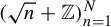
 $\alpha = \tfrac {1}{2}$
, as shown in Figure 1.
$\alpha = \tfrac {1}{2}$
, as shown in Figure 1.

Figure 1 The proportion of $N = 10\,000\,000$
intervals in partition of
$N = 10\,000\,000$
intervals in partition of $\mathbb {T}$
containing
$\mathbb {T}$
containing $0 \leq j \leq 6$
points of
$0 \leq j \leq 6$
points of $n^{\alpha } + \mathbb {Z}$
for
$n^{\alpha } + \mathbb {Z}$
for $n \leq N$
when
$n \leq N$
when $\alpha $
is equal to
$\alpha $
is equal to $\tfrac {1}{2}$
,
$\tfrac {1}{2}$
, $\tfrac {1}{3}$
and
$\tfrac {1}{3}$
and $\tfrac {2}{3}$
. For
$\tfrac {2}{3}$
. For $\alpha =1/2$
, these proportions approximate
$\alpha =1/2$
, these proportions approximate $E_j(s)$
for
$E_j(s)$
for $s = 1$
.
$s = 1$
.
We can also recast our problem in a probabilistic setting. Indeed, for $N \in \mathbb {N}$
, let
$N \in \mathbb {N}$
, let $W_N$
be a random variable which is distributed uniformly on the set
$W_N$
be a random variable which is distributed uniformly on the set $\Omega _N$
. Then, we define a sequence of stochastic processes
$\Omega _N$
. Then, we define a sequence of stochastic processes $Y^N_s$
for
$Y^N_s$
for $N \in \mathbb {N}$
and
$N \in \mathbb {N}$
and $s \geq 0$
by setting
$s \geq 0$
by setting
 $$ \begin{align} Y^N_s := S_N(W_N,s). \end{align} $$
With this notation, Theorem 1.1 states that the sequence $\mathbb {P}(Y^N_s = j)$
converges as
$\mathbb {P}(Y^N_s = j)$
converges as $N \to \infty $
.
$N \to \infty $
.
For each N, we can also think about each point $x_0 \in \Omega _N$
as giving us a locally finite Borel measure on
$x_0 \in \Omega _N$
as giving us a locally finite Borel measure on $\mathbb {R}^+$
of the form
$\mathbb {R}^+$
of the form
 $$ \begin{align*} \eta_N(x_0) := \sum_{r=1}^{\infty} \delta_{s_r(x_0)}, \end{align*} $$
where $s_1(x_0) < s_2(x_0) < s_3(x_0), \ldots , $
are the complete sequence of points
$s_1(x_0) < s_2(x_0) < s_3(x_0), \ldots , $
are the complete sequence of points $s \in ({1}/{N})\mathbb {N}$
such that
$s \in ({1}/{N})\mathbb {N}$
such that $\sqrt {sN} \in [x_0- {1}/{2N}, x_0 + {1}/{2N} ) + \mathbb {Z} $
. Namely, these are points of discontinuity of the map
$\sqrt {sN} \in [x_0- {1}/{2N}, x_0 + {1}/{2N} ) + \mathbb {Z} $
. Namely, these are points of discontinuity of the map $s \longmapsto S_N(x_0,s)$
. In this case, we have the relation
$s \longmapsto S_N(x_0,s)$
. In this case, we have the relation
 $$ \begin{align} \eta_N(x_0)([0,s]) = S_N(x_0,s). \end{align} $$
Again, recasting this in a probabilistic setting, we define the corresponding sequence of random measures/point processes $\xi _N$
by setting
$\xi _N$
by setting
 $$ \begin{align} \xi_N := \eta_N(W_N). \end{align} $$
Equation (1.5) above tells us that for an interval $(a,b] \subset \mathbb {R}^+$
, we have that the point process and stochastic process are related via
$(a,b] \subset \mathbb {R}^+$
, we have that the point process and stochastic process are related via
 $$ \begin{align} \xi_N((a,b]) = Y^N_b - Y^N_a\!. \end{align} $$
In this setting, we establish the following convergence result which helps us to understand how the limiting distribution of the points of our sequence varies with s.
Theorem 1.5. The point process $(\xi _N)_{N=1}^{\infty }$
converges in distribution to a point process
$(\xi _N)_{N=1}^{\infty }$
converges in distribution to a point process $\xi $
.
$\xi $
.
The process $\xi $
is defined similarly to the processes
$\xi $
is defined similarly to the processes $\xi _N$
as the sum of Dirac delta measures associated to the jump points of a stochastic process
$\xi _N$
as the sum of Dirac delta measures associated to the jump points of a stochastic process $Y_s:X \to \mathbb {R}$
. Here the space X can be the thought of as the homogeneous space of all two-dimensional affine unimodular lattices (which we show explicitly in §2) and
$Y_s:X \to \mathbb {R}$
. Here the space X can be the thought of as the homogeneous space of all two-dimensional affine unimodular lattices (which we show explicitly in §2) and $Y_s(x)$
gives the number of points of the lattice associated to
$Y_s(x)$
gives the number of points of the lattice associated to $x\in X$
within a certain triangle of areas s in the plane. More concretely, if the lattice associated to
$x\in X$
within a certain triangle of areas s in the plane. More concretely, if the lattice associated to $x \in X$
is
$x \in X$
is $L \subset \mathbb {R}^2$
and
$L \subset \mathbb {R}^2$
and
 $$ \begin{align} \tau(\infty) := \{ (u,v) \in \mathbb{R}^2: u \geq 0, -u\leq v \leq u \}, \end{align} $$
then
 $$ \begin{align} \xi(x) = \sum_{(u,v) \in L \cup \tau(\infty) } \delta_{\sqrt{u}}. \end{align} $$
As we illustrate in §6, $\xi $
is a simple, intensity-1 process which does not have independent increments.
$\xi $
is a simple, intensity-1 process which does not have independent increments.
Remark 1.6. The pigeonhole statistics we consider were previously studied by Weiss and Peres for the fractional parts of the sequence $2^n \alpha $
(as well as higher dimensional generalisations). In this case, the analogous processes converge to a Poisson point process [Reference Weiss19]. A Poisson point process is also (almost surely) the limiting process we would obtain if, instead of generating our point processes via considering how the points of the sequence
$2^n \alpha $
(as well as higher dimensional generalisations). In this case, the analogous processes converge to a Poisson point process [Reference Weiss19]. A Poisson point process is also (almost surely) the limiting process we would obtain if, instead of generating our point processes via considering how the points of the sequence $\sqrt {n}$
distribute among shrinking partitions of
$\sqrt {n}$
distribute among shrinking partitions of $\mathbb {T}$
, we instead consider the analogous processes defined for a sequence of points in
$\mathbb {T}$
, we instead consider the analogous processes defined for a sequence of points in $\mathbb {T}$
generated by a sequence of independent and identically distributed random variables which are uniformly distributed on
$\mathbb {T}$
generated by a sequence of independent and identically distributed random variables which are uniformly distributed on $\mathbb {T}$
[Reference Feller8, §VI.6].
$\mathbb {T}$
[Reference Feller8, §VI.6].
Similarly to what is observed in [Reference El-Baz, Marklof and Vinogradov6], even though our limiting processes is not Poissonian, its second moment is nearly Poissonian with an error resulting from the fact that, asymptotically, $\sqrt {N}$
of the points
$\sqrt {N}$
of the points $\{ \sqrt {n} + \mathbb {Z} : 1 \leq n \leq N \}$
are
$\{ \sqrt {n} + \mathbb {Z} : 1 \leq n \leq N \}$
are $0$
.
$0$
.
Corollary 1.7.
 $$ \begin{align*} \mathbb{E}[|Y^N_s|^2] \to \sum_{j=0}^{\infty} j^2E_j(s)^2 + s =\int_X |Y_s|^2 \; dm_X + s = s^2 + 2s \end{align*} $$
as $N \to \infty $
. In particular,
$N \to \infty $
. In particular,
 $$ \begin{align*} \mathrm{Var}[Y^N_s] \to 2s \end{align*} $$
as $N \to \infty $
.
$N \to \infty $
.
Remark 1.8. If we desire the (more satisfactory) convergence of the variance of the random variables $Y^N_s$
to those of
$Y^N_s$
to those of $Y_s$
, one has to avoid the escape of mass resulting from the term
$Y_s$
, one has to avoid the escape of mass resulting from the term $0$
appearing regularly in the sequence of fractional parts of
$0$
appearing regularly in the sequence of fractional parts of $\sqrt {n}$
. This can be done via removing the terms
$\sqrt {n}$
. This can be done via removing the terms $\sqrt {n}$
when n is a square and, in this case, we would have Var
$\sqrt {n}$
when n is a square and, in this case, we would have Var $[Y^N_s] \to s$
which is the variance we would obtain if the limiting point process were Poissonian. We will also use this approach in the proof of Corollary 1.7.
$[Y^N_s] \to s$
which is the variance we would obtain if the limiting point process were Poissonian. We will also use this approach in the proof of Corollary 1.7.
1.1 Ergodic theory
Let $G = \text {ASL}(2,\mathbb {R}) = \text {SL}(2,\mathbb {R})\ltimes \mathbb {R}^2$
be the affine special linear group of
$G = \text {ASL}(2,\mathbb {R}) = \text {SL}(2,\mathbb {R})\ltimes \mathbb {R}^2$
be the affine special linear group of $\mathbb {R}^2$
with multiplication law defined by
$\mathbb {R}^2$
with multiplication law defined by
 $$ \begin{align*} (M,x)(M', x') = (MM',xM' + x'), \end{align*} $$
where elements of $\mathbb {R}^2$
are viewed as row vectors. Let
$\mathbb {R}^2$
are viewed as row vectors. Let $ \Gamma = \text {SL}(2,\mathbb {Z}) \ltimes \mathbb {Z}^2$
be the discrete subgroup of G consisting of elements with integer entries. As is discussed in §2,
$ \Gamma = \text {SL}(2,\mathbb {Z}) \ltimes \mathbb {Z}^2$
be the discrete subgroup of G consisting of elements with integer entries. As is discussed in §2, $\Gamma $
is a lattice in G, meaning we have a fundamental domain
$\Gamma $
is a lattice in G, meaning we have a fundamental domain $\widetilde {\mathcal {F}}$
with finite volume (and hence, up to normalization, volume 1) under the Haar measure
$\widetilde {\mathcal {F}}$
with finite volume (and hence, up to normalization, volume 1) under the Haar measure $m_G$
on G. By restricting
$m_G$
on G. By restricting $m_G$
to
$m_G$
to $\widetilde {\mathcal {F}}$
and projecting to X, we have a right-invariant probability measure
$\widetilde {\mathcal {F}}$
and projecting to X, we have a right-invariant probability measure $m_X$
on the space
$m_X$
on the space $X: = \Gamma \backslash G$
which we call the Haar measure on X [Reference Einsiedler and Ward4, Proposition 9.20]. Let
$X: = \Gamma \backslash G$
which we call the Haar measure on X [Reference Einsiedler and Ward4, Proposition 9.20]. Let
 $$ \begin{align*} \Phi(t) := \bigg( \begin{pmatrix} e^{-{t}/{2}} & 0 \\ 0 & e^{{t}/{2}} \end{pmatrix} , (0,0) \bigg) \end{align*} $$
and
 $$ \begin{align*} a(N) := \Phi(\log(N)). \end{align*} $$
As in [Reference Elkies and McMullen7], we shall be concerned with the equidistribution of points on certain horocycle sections in the space X. Here, a horocycle section is a function $\sigma :\mathbb {R} \to G$
of the form
$\sigma :\mathbb {R} \to G$
of the form
 $$ \begin{align*} \sigma(t) := \bigg( \begin{pmatrix} 1 & 2t \\ 0 & 1 \end{pmatrix} , (x(t),y(t)) \bigg), \end{align*} $$
where $x(t)$
and
$x(t)$
and $y(t)$
are smooth functions. We call
$y(t)$
are smooth functions. We call $\sigma (t)$
a horocycle section of period
$\sigma (t)$
a horocycle section of period $p \in \mathbb {N}$
if there exists some
$p \in \mathbb {N}$
if there exists some $\gamma _0 \in \Gamma $
such that
$\gamma _0 \in \Gamma $
such that $\gamma _0 \sigma (t + p) = \gamma _0 \sigma (t)$
for all
$\gamma _0 \sigma (t + p) = \gamma _0 \sigma (t)$
for all $t \in \mathbb {R}$
. Moreover, such a horocycle section is nonlinear if there exists some
$t \in \mathbb {R}$
. Moreover, such a horocycle section is nonlinear if there exists some $\alpha , \beta \in \mathbb {Q}$
such that the set
$\alpha , \beta \in \mathbb {Q}$
such that the set $\{ t \in [0,p] : y(t) = \alpha t + \beta \}$
has zero Lebesgue measure. For such horocycle sections, the following equidistribution result is known.
$\{ t \in [0,p] : y(t) = \alpha t + \beta \}$
has zero Lebesgue measure. For such horocycle sections, the following equidistribution result is known.
Theorem 1.9. [Reference Elkies and McMullen7, Theorem 2.2], [Reference Marklof12, Theorem 4.2]
Let $\sigma $
be a nonlinear horocycle section with period p. Then, for any bounded continuous function
$\sigma $
be a nonlinear horocycle section with period p. Then, for any bounded continuous function $f:X \to \mathbb {R}$
,
$f:X \to \mathbb {R}$
,
 $$ \begin{align*} \frac{1}{p}\int_0^p f(\Gamma \sigma(x_0) \Phi(t)) \; dx_0 \to \int_X f \; dm_X \end{align*} $$
as $t \to \infty $
.
$t \to \infty $
.
Applying this to the nonlinear period 1 horocycle section
 $$ \begin{align*} n(t) := \bigg( \begin{pmatrix} 1 & 2t \\ 0 & 1 \end{pmatrix} , (t,t^2) \bigg), \end{align*} $$
one can determine the distribution of $\{ \sqrt {n}\}_{n=1}^N$
among the intervals
$\{ \sqrt {n}\}_{n=1}^N$
among the intervals $[x_0 - 1/2N, x_0 + 1/2N) + \mathbb {Z}$
when
$[x_0 - 1/2N, x_0 + 1/2N) + \mathbb {Z}$
when $x_0$
is uniformly distributed on
$x_0$
is uniformly distributed on $[0,1)$
. In our setting, we restrict
$[0,1)$
. In our setting, we restrict $x_0$
to lying in the set
$x_0$
to lying in the set $\Omega _N$
for each N and the corresponding equidistribution we desire is that of rational points on such a horocycle section. We therefore prove the following result which, like Theorem 1.9, applies more generally to functions
$\Omega _N$
for each N and the corresponding equidistribution we desire is that of rational points on such a horocycle section. We therefore prove the following result which, like Theorem 1.9, applies more generally to functions $f:X \to \mathbb {R}$
which are piecewise continuous: functions
$f:X \to \mathbb {R}$
which are piecewise continuous: functions $f:X \to \mathbb {R}$
whose points of discontinuity are contained in a set of measure zero with respect to
$f:X \to \mathbb {R}$
whose points of discontinuity are contained in a set of measure zero with respect to $m_X$
.
$m_X$
.
Theorem 1.10. Let $\sigma $
be a nonlinear horocycle section with period p. Then, for any bounded piecewise continuous function
$\sigma $
be a nonlinear horocycle section with period p. Then, for any bounded piecewise continuous function $f:X \to \mathbb {R}$
and
$f:X \to \mathbb {R}$
and $C \geq 1$
,
$C \geq 1$
,
 $$ \begin{align} \frac{1}{pN} \sum_{k=0}^{pN-1} f\bigg(\Gamma \sigma\bigg( \frac{k}{N}\bigg)a(M) \bigg) \to \int_X f \; dm_X \end{align} $$
as $N \to \infty $
and
$N \to \infty $
and ${1}/{C}N \leq M \leq CN$
.
${1}/{C}N \leq M \leq CN$
.
As we show concretely in §5, for an appropriate $f:X \to \mathbb {R}$
, we can approximate
$f:X \to \mathbb {R}$
, we can approximate $\mathbb {P}(\xi _N((a,b]) = 0)$
(or more generally
$\mathbb {P}(\xi _N((a,b]) = 0)$
(or more generally $ \mathbb {P}(\xi _N(B) = 0)$
for B as in Lemma 1.13(ii)) by a sum of the above form in equation (1.10) and, using the above equidistribution result, show Theorem 1.5. The same principle applies in the case of Theorem 1.1.
$ \mathbb {P}(\xi _N(B) = 0)$
for B as in Lemma 1.13(ii)) by a sum of the above form in equation (1.10) and, using the above equidistribution result, show Theorem 1.5. The same principle applies in the case of Theorem 1.1.
Remark 1.11. Although Theorems 1.1, 1.5 and 1.10 are stated for the points/interval centres ${k}/{N}$
for
${k}/{N}$
for $0 \leq k \leq N-1$
, one can see the methods presented in this paper also give the analogous results when considering the points/interval centres
$0 \leq k \leq N-1$
, one can see the methods presented in this paper also give the analogous results when considering the points/interval centres $({k+ \alpha })/{N}$
for any
$({k+ \alpha })/{N}$
for any $\alpha \in \mathbb {R} $
. The choice
$\alpha \in \mathbb {R} $
. The choice $\alpha = \tfrac {1}{2}$
in particular results in considering the points of the sequence
$\alpha = \tfrac {1}{2}$
in particular results in considering the points of the sequence $\sqrt {n}$
in the intervals formed via partitioning by cutting
$\sqrt {n}$
in the intervals formed via partitioning by cutting $\mathbb {T}$
at the points
$\mathbb {T}$
at the points ${k}/{N}$
for
${k}/{N}$
for $0 \leq k \leq N-1$
.
$0 \leq k \leq N-1$
.
Remark 1.12. There are many known results related to Theorem 1.10 when considering the equidistribution of discrete collections of points on expanding horocycle orbits. An effective equidistribution theorem for rational horocycle points $\{ k/N + iy \}_{k=0}^{N-1}$
in the modular surface is proved by Burrin, Shapira and Yu in [Reference Burrin, Shapira and Yu1, Theorem 1.1]. Using spectral methods, [Reference Burrin, Shapira and Yu1] shows such points equidistribute when the number of such rational points N being considered at height y satisfies
$\{ k/N + iy \}_{k=0}^{N-1}$
in the modular surface is proved by Burrin, Shapira and Yu in [Reference Burrin, Shapira and Yu1, Theorem 1.1]. Using spectral methods, [Reference Burrin, Shapira and Yu1] shows such points equidistribute when the number of such rational points N being considered at height y satisfies $N \gg y^{-({39}/{64} + \epsilon )}$
for some
$N \gg y^{-({39}/{64} + \epsilon )}$
for some $\epsilon> 0$
. This contrasts with Theorem 1.10, which corresponds to the case when
$\epsilon> 0$
. This contrasts with Theorem 1.10, which corresponds to the case when $N \asymp y^{-1}$
. Using dynamical methods, Einsiedler, Luethi and Shah prove effective equistribution results for the rational points
$N \asymp y^{-1}$
. Using dynamical methods, Einsiedler, Luethi and Shah prove effective equistribution results for the rational points
 $$ \begin{align*} \bigg\{ \bigg(\text{SL}(2,\mathbb{Z}) \begin{pmatrix} 1 & k/N \\ 0 & 1 \end{pmatrix} \begin{pmatrix} N^{-1/2} & 0 \\ 0 & N^{1/2} \end{pmatrix}, \frac{k}{N} + \mathbb{Z}\bigg) : 0 \leq K \leq N-1 \bigg\} \end{align*} $$
in the more general space SL $(2,\mathbb {Z}) \backslash $
SL
$(2,\mathbb {Z}) \backslash $
SL $(2,\mathbb {R}) \times \mathbb {T}$
[Reference Einsiedler, Luethi and Shah3]. The equidistribution of such points when projected SL
$(2,\mathbb {R}) \times \mathbb {T}$
[Reference Einsiedler, Luethi and Shah3]. The equidistribution of such points when projected SL $(2,\mathbb {Z}) \backslash $
SL
$(2,\mathbb {Z}) \backslash $
SL $(2,\mathbb {R})$
is implied by Theorem 1.10. Finally, in [Reference Marklof and Strömbergsson13], Marklof and Strömbergsson prove for fixed
$(2,\mathbb {R})$
is implied by Theorem 1.10. Finally, in [Reference Marklof and Strömbergsson13], Marklof and Strömbergsson prove for fixed $\delta> 0$
, there is full measure set of
$\delta> 0$
, there is full measure set of $\alpha \in [0,1)$
such that the points
$\alpha \in [0,1)$
such that the points $\{m\alpha + iy\}_{m=1}^N$
equidistribute in the modular surface as
$\{m\alpha + iy\}_{m=1}^N$
equidistribute in the modular surface as $y \to 0$
whenever
$y \to 0$
whenever ${y \asymp N^{-\delta }}$
.
${y \asymp N^{-\delta }}$
.
1.2 Outline of proof
Recall the following conditions which are sufficient to give the convergence in distribution of a sequence of point processes [Reference Leadbetter, Lindgren and Rootzén11, Theorem A2.2].
Lemma 1.13. [Reference Leadbetter, Lindgren and Rootzén11, Theorem A2.2]
Let $(\xi _n)_{n=1}^{\infty }$
and
$(\xi _n)_{n=1}^{\infty }$
and $\xi $
be point processes defined on
$\xi $
be point processes defined on $ \mathbb {R}^+$
with
$ \mathbb {R}^+$
with $\xi $
being simple. Suppose the following:
$\xi $
being simple. Suppose the following:
-
(i) $\mathbb {E}[ \xi _N((a,b]) ] \to \mathbb {E}[ \xi ((a,b]) ] $
as
$N \to \infty $
for all
$0 \leq a < b < \infty $
;
$\mathbb {E}[ \xi _N((a,b]) ] \to \mathbb {E}[ \xi ((a,b]) ] $
as
$N \to \infty $
for all
$0 \leq a < b < \infty $
; -
(ii)
$ \mathbb {P}[\xi _N(V) = 0 ] \to \mathbb {P}[(\xi (V) = 0 ] $
for all V of the form
$ \bigcup _{j=1}^k (a_j,b_j]$
with
$0 \leq a_1 < b_1 \leq a_2 < b_2 \leq \cdots \leq a_k < b_k$
.


Then $\xi _N \xrightarrow {d} \xi $
, where
$\xi _N \xrightarrow {d} \xi $
, where $\xrightarrow {d}$
denotes convergence in distribution.
$\xrightarrow {d}$
denotes convergence in distribution.
For our processes $\xi _N$
defined by equation (1.6), we will see that condition (i) merely amounts to the fact the average number of points of an affine unimodular lattice in a triangle of area s is s. We prove this more generally in Lemma 5.1.
$\xi _N$
defined by equation (1.6), we will see that condition (i) merely amounts to the fact the average number of points of an affine unimodular lattice in a triangle of area s is s. We prove this more generally in Lemma 5.1.
Turning to (ii), we define the measures $(\nu _N)_{n=1}^{\infty }$
on X by
$(\nu _N)_{n=1}^{\infty }$
on X by
 $$ \begin{align} \nu_N(f) = \int_X f \; d\nu_N := \frac{1}{N} \sum_{k=0}^{N-1} f\bigg(\Gamma n\bigg( \frac{k}{N}\bigg)a(N) \bigg). \end{align} $$
In §5, for a given set V as in Lemma 1.13(ii), we show how to choose the function $f :X \to \mathbb {R}$
such that
$f :X \to \mathbb {R}$
such that $\nu _N(f)$
approximates
$\nu _N(f)$
approximates $\mathbb {P}(\xi _N(B) = 0)$
. The same is true in proving Theorem 1.1, where we choose a function
$\mathbb {P}(\xi _N(B) = 0)$
. The same is true in proving Theorem 1.1, where we choose a function $f:X \to \mathbb {R}$
such that
$f:X \to \mathbb {R}$
such that $\nu _N(f)$
approximates
$\nu _N(f)$
approximates $\mathbb {P}(Y^N_s = j)$
. By taking
$\mathbb {P}(Y^N_s = j)$
. By taking $N \to \infty $
, we can then show the required limiting values are attained using Theorem 1.10. For the remainder of this section, we thus focus on the proof of Theorem 1.10.
$N \to \infty $
, we can then show the required limiting values are attained using Theorem 1.10. For the remainder of this section, we thus focus on the proof of Theorem 1.10.
Proof outline of Theorem 1.10 for
$\sigma (t) = n(t)$

By a standard approximation argument, it suffices to show we have $\nu _N(f) \to \int _X f \; dm_X$
for all
$\nu _N(f) \to \int _X f \; dm_X$
for all $f \in C_c(X)$
. This allows us to reduce to understanding weak-star limit points of the sequence of measure
$f \in C_c(X)$
. This allows us to reduce to understanding weak-star limit points of the sequence of measure $(\nu _N)$
. In particular it suffices, by the Banach–Alaoglu theorem, to show any accumulation point
$(\nu _N)$
. In particular it suffices, by the Banach–Alaoglu theorem, to show any accumulation point $\nu $
of the measures
$\nu $
of the measures $(\nu _N)$
is
$(\nu _N)$
is $m_X$
.
$m_X$
.
As is shown in Proposition 3.1, moving from $n({k}/{N})a(N)$
to
$n({k}/{N})a(N)$
to $n(({k+1})/{N})a(N)$
corresponds, up to some negligible error, to right multiplication by the unipotent element
$n(({k+1})/{N})a(N)$
corresponds, up to some negligible error, to right multiplication by the unipotent element $u(1)$
, where
$u(1)$
, where
 $$ \begin{align} u(t) := \bigg( \begin{pmatrix} 1 & 2t \\ 0 & 1 \end{pmatrix} , (0,0) \bigg) \end{align} $$
for $t \in \mathbb {R}$
. It will follow that any such
$t \in \mathbb {R}$
. It will follow that any such $\nu $
is invariant under the action of the subgroup
$\nu $
is invariant under the action of the subgroup $\{u(k)\}_{k \in \mathbb {Z}}$
.
$\{u(k)\}_{k \in \mathbb {Z}}$
.
The right-action of this subgroup on X is mixing, as is shown in Lemma 3.4. A consequence of this is that the system $(X,U_t,m_X)$
, where
$(X,U_t,m_X)$
, where $U_t(x) = xu(t)$
, is disjoint from the linear rotation flow on
$U_t(x) = xu(t)$
, is disjoint from the linear rotation flow on $[0,1)$
in the sense introduced by Furstenberg in [Reference Furstenberg9] (as is shown in Lemma 3.3). To be precise, the linear rotation flow
$[0,1)$
in the sense introduced by Furstenberg in [Reference Furstenberg9] (as is shown in Lemma 3.3). To be precise, the linear rotation flow $R_t:[0,1) \to [0,1)$
is given by
$R_t:[0,1) \to [0,1)$
is given by $R_t(s) = \{s+t\}$
, where
$R_t(s) = \{s+t\}$
, where $\{ \cdot \}$
gives the fractional part of a real number. This is used to extend to the flow
$\{ \cdot \}$
gives the fractional part of a real number. This is used to extend to the flow $U_t$
to
$U_t$
to $\widetilde {U}_t: X \times [0,1)\to X \times [0,1)$
given by
$\widetilde {U}_t: X \times [0,1)\to X \times [0,1)$
given by $\widetilde {U}_t(\Gamma g,s) = (\Gamma g u(t),\{s+t\})$
. Disjointness then tells us that the only
$\widetilde {U}_t(\Gamma g,s) = (\Gamma g u(t),\{s+t\})$
. Disjointness then tells us that the only $\widetilde {U}_t$
-invariant measure on
$\widetilde {U}_t$
-invariant measure on $ X \times [0,1) $
whole marginals (projections to X and
$ X \times [0,1) $
whole marginals (projections to X and $[0,1)$
) are
$[0,1)$
) are $m_X$
, and the Lebesgue measure
$m_X$
, and the Lebesgue measure $ds$
on
$ds$
on $[0,1)$
is the product measure
$[0,1)$
is the product measure $m_X \times ds$
.
$m_X \times ds$
.
To use this fact, we consider the corresponding special flow under the ceiling function $1$
: namely, the flow
$1$
: namely, the flow $T_t:X \times [0,1) \to X \times [0,1)$
given by
$T_t:X \times [0,1) \to X \times [0,1)$
given by
 $$ \begin{align*} T_t(\Gamma g,s) = (\Gamma g u(\lfloor s + t \rfloor ), \lbrace s+t \rbrace ). \end{align*} $$
This flow has $\nu \times ds$
as an invariant measure and is also conjugate to the flow
$\nu \times ds$
as an invariant measure and is also conjugate to the flow $\widetilde {U}_t$
. Keeping track of the measure
$\widetilde {U}_t$
. Keeping track of the measure $\nu \times ds$
under this conjugation map (described explicitly in the proof of Proposition 3.6) and using Theorem 1.9, we see the resulting measure on
$\nu \times ds$
under this conjugation map (described explicitly in the proof of Proposition 3.6) and using Theorem 1.9, we see the resulting measure on $X \times [0,1)$
indeed has marginals
$X \times [0,1)$
indeed has marginals $m_X$
and
$m_X$
and $ds$
, and so is the product measure
$ds$
, and so is the product measure $m_X \times ds$
. This in turn gives us that
$m_X \times ds$
. This in turn gives us that $\nu \times ds = m_X \times ds$
by applying the inverse of the conjugation map and so
$\nu \times ds = m_X \times ds$
by applying the inverse of the conjugation map and so $\nu = m_X$
, as required.
$\nu = m_X$
, as required.
2 The space X
Here we overview, for completeness, some of the basic properties of the space $X = \Gamma \backslash G$
which we will be using. More details can be found in [Reference Marklof12, §3.1] and [Reference Strömbergsson16, §1].
$X = \Gamma \backslash G$
which we will be using. More details can be found in [Reference Marklof12, §3.1] and [Reference Strömbergsson16, §1].
-
• X is a
$\mathbb {T}^2 = \mathbb {R}^2 / \mathbb {Z}^2 $
bundle over the base space
$B :=\text {SL}(2,\mathbb {Z}) \backslash \text {SL}(2,\mathbb {R})$
. If
$\mathcal {F}$
is a fundamental domain for the left-action of SL
$(2,\mathbb {Z})$
on SL
$(2,\mathbb {R})$
, then a fundamental domain for the left-action of
$\Gamma $
on G is We fix such
$$ \begin{align*} \widetilde{\mathcal{F}} &= \{ (I_2,x)(M,0) : x \in [0,1), M \in \mathcal{F} \} \\ &= \{ (M,x) \in G : M \in F \text{ and } x \in [0,1)^2M \}. \end{align*} $$
$\mathcal {F}$
and
$\widetilde {\mathcal {F}}$
for the remainder of paper.
-
• Let
$m_{\text {SL}(2,\mathbb {R})}$
be the Haar measure on the unimodular group
$\text {SL}(2,\mathbb {R})$
, normalised so that
$m_{\text {SL}(2,\mathbb {R})}(\mathcal {F}) = 1$
. Using Fubini’s theorem and the translation invariance, it is easy to see
$m_G = m_{\text {SL}(2,\mathbb {R})} \times dx$
is a (left) Haar measure on X, where
$dx$
represents the Lebesgue measure on
$\mathbb {R}^2$
. The right-invariant measure
$m_X$
on X is obtained by then restricting this measure
$m_G$
to
$\widetilde {\mathcal {\mathcal {F}}}$
. -
• There exists a left-invariant Reimannian metric
$d_G$
on G inducing the same topology on G as the product topology on the space SL
$(2,\mathbb {R}) \times \mathbb {R}^2$
. Fixing one such metric
$d_G$
, we construct a metric d on X via defining For more explicit details on these constructions, see [Reference Einsiedler and Ward4, §9.3]. Throughout the remaining sections, continuity of functions
$$ \begin{align*} d(\Gamma g_1, \Gamma g_2) := \inf_{\gamma \in \Gamma} d_G(\gamma g_1,g_2). \end{align*} $$
$f:X \to \mathbb {R}$
will mean continuity with respect to this metric.
-
• Any element
$(M, x) \in G$
gives us an affine unimodular lattice in
$\mathbb {R}^2$
—namely the lattice
$\mathbb {Z}^2M + x$
. Moreover, for any other
$(M', x') \in G$
, the lattice associated to
$(M',x')(M, x)$
is given by
$\mathbb {Z}^2M'M + x'M + x$
. These two lattices are identical if and only if
$(M' ,x') \in \Gamma $
. Thus we have a natural identification between elements of
$X = \Gamma \backslash G$
and such lattices. We will use this identification in §5 to construct the functions
$f:X \to \mathbb {R}$
to which we will apply Theorem 1.10.


3 The special flow under
$1$

Throughout this section, whenever $(X_1, \mu _1)$
is a measure space,
$(X_1, \mu _1)$
is a measure space, $X_2$
is a measurable space and
$X_2$
is a measurable space and $\mathcal {T}:X_1 \to X_2$
is a measurable map, we will define the measure
$\mathcal {T}:X_1 \to X_2$
is a measurable map, we will define the measure $\mathcal {T}_{*}\mu _1$
on
$\mathcal {T}_{*}\mu _1$
on $X_2$
by
$X_2$
by
 $$ \begin{align*} \mathcal{T}_{*}\mu_1(A) = \mu_1(\mathcal{T}^{-1}(A)) \end{align*} $$
for any measurable $A \subset X_2$
.
$A \subset X_2$
.
Proposition 3.1. Let $\sigma $
be a nonlinear horocycle section of period p. Define the measures
$\sigma $
be a nonlinear horocycle section of period p. Define the measures $(\nu _N)_{n=1}^{\infty }$
on X by setting
$(\nu _N)_{n=1}^{\infty }$
on X by setting
 $$ \begin{align} \nu_N(f) = \int_X f \; d\nu_N := \frac{1}{pN} \sum_{k=0}^{pN-1} f\bigg(\Gamma \sigma\bigg( \frac{k}{N}\bigg)a(N) \bigg) \end{align} $$
for any continuous bounded $f:X \to \mathbb {C}$
. Then, any weak-star limit point of the measures defined in equation (3.1) is invariant under the map
$f:X \to \mathbb {C}$
. Then, any weak-star limit point of the measures defined in equation (3.1) is invariant under the map $T:X \to X$
given by
$T:X \to X$
given by
 $$ \begin{align} T(\Gamma g) = \Gamma g u(1), \end{align} $$
where $u(1)$
is defined by equation (1.12).
$u(1)$
is defined by equation (1.12).
To see this, we will need the following lemma.
Lemma 3.2. Any $f \in C_c(X)$
is uniformly continuous in the
$f \in C_c(X)$
is uniformly continuous in the $\mathbb {T}^2$
direction. More precisely, for any
$\mathbb {T}^2$
direction. More precisely, for any $\epsilon> 0$
, we can find
$\epsilon> 0$
, we can find $\delta> 0$
such that for all
$\delta> 0$
such that for all $M \in {\textrm {SL}}(2,\mathbb {R})$
and
$M \in {\textrm {SL}}(2,\mathbb {R})$
and $u,v \in \mathbb {T}^2$
with
$u,v \in \mathbb {T}^2$
with $d_{\mathbb {T}^2}(u,v) \leq \delta $
, we have
$d_{\mathbb {T}^2}(u,v) \leq \delta $
, we have
 $$ \begin{align*} | f((I_2,u)(M,0)) - f((I_2,v)(M,0)) | < \epsilon. \end{align*} $$
Proof. Take $f \in C_c(X)$
and let K be the projection of the support of f to the base space
$f \in C_c(X)$
and let K be the projection of the support of f to the base space $B $
. Here, K is a compact set and so the map
$B $
. Here, K is a compact set and so the map $K \times \mathbb {T}^2 \ni (M,x) \longmapsto f((I_2,x)(M,0)) \in \mathbb {R}$
is uniformly continuous. This means f is uniformly continuous in the fibre direction over K in the sense that for any
$K \times \mathbb {T}^2 \ni (M,x) \longmapsto f((I_2,x)(M,0)) \in \mathbb {R}$
is uniformly continuous. This means f is uniformly continuous in the fibre direction over K in the sense that for any $\epsilon> 0$
, we can find
$\epsilon> 0$
, we can find $\delta> 0$
such that for any
$\delta> 0$
such that for any $M \in K$
and
$M \in K$
and $u,v \in \mathbb {T}^2$
with
$u,v \in \mathbb {T}^2$
with $d_{\mathbb {T}^2}(u,v) < \delta $
, we have
$d_{\mathbb {T}^2}(u,v) < \delta $
, we have
 $$ \begin{align*} | f((I_2,u)(M,0)) - f((I_2,v)(M,0)) | < \epsilon. \end{align*} $$
Hence, since f is identically zero on the fibre above all base points outside of K, f is in fact uniformly continuous in the fibre direction over all of $B $
.
$B $
.
Proof of Proposition 3.1
Suppose $\nu $
is a weak-star limit of the sequence of measures
$\nu $
is a weak-star limit of the sequence of measures $(\nu _{N_j})$
where
$(\nu _{N_j})$
where $N_j \nearrow \infty $
.
$N_j \nearrow \infty $
.
Now, for any $N \in \mathbb {N}$
and
$N \in \mathbb {N}$
and $0 \leq k \leq pN-1$
, we will see via equations (3.3) and (3.4) that the two points
$0 \leq k \leq pN-1$
, we will see via equations (3.3) and (3.4) that the two points $ \sigma (({k+1})/{N})a(N)$
and
$ \sigma (({k+1})/{N})a(N)$
and $ \sigma ({k}/{N})a(N)u(1) $
are identical in their SL
$ \sigma ({k}/{N})a(N)u(1) $
are identical in their SL $(2,\mathbb {R})$
components and, as the functions x and y are smooth and so bounded and Lipschitz on
$(2,\mathbb {R})$
components and, as the functions x and y are smooth and so bounded and Lipschitz on $[0,p]$
, differ by a distance
$[0,p]$
, differ by a distance $O({1}/{N} )$
in the
$O({1}/{N} )$
in the $ \mathbb {T}^2$
direction. Using this, we will see the measures
$ \mathbb {T}^2$
direction. Using this, we will see the measures $\{T_{*}\nu _{N_j}\}_{j \in \mathbb {N}}$
given by
$\{T_{*}\nu _{N_j}\}_{j \in \mathbb {N}}$
given by
 $$ \begin{align*} T_{*}\nu_{N_j}(f) = \frac{1}{pN_j} \sum_{k=0}^{pN_j-1} f\bigg(\Gamma \sigma\bigg(\frac{k}{N_j}\bigg)a(N_j)u(1)\bigg), \quad f \in C_c(X) \end{align*} $$
will also converge to $\nu $
as
$\nu $
as $j \to \infty $
in the weak-star topology, since, for compactness,
$j \to \infty $
in the weak-star topology, since, for compactness, $f \in C_c(X)$
,
$f \in C_c(X)$
, $f(\sigma ({k}/{N_j})a(N_j)u(1))$
and
$f(\sigma ({k}/{N_j})a(N_j)u(1))$
and $f(\sigma (({k+1})/{N})a(N))$
will be uniformly close across all
$f(\sigma (({k+1})/{N})a(N))$
will be uniformly close across all $0 \leq k \leq pN_j-1$
in equation (3.5). This will follow from the Lemma 3.2.
$0 \leq k \leq pN_j-1$
in equation (3.5). This will follow from the Lemma 3.2.
Indeed, we have
 $$ \begin{align} \sigma\bigg(\frac{k+1}{N}\bigg)a(N) &= \bigg(\!\! \begin{pmatrix} N^{-1/2} & 2(k+1)N^{-1/2} \\ 0 & N^{1/2} \end{pmatrix}\! , \bigg( x\bigg(\frac{k+1}{N}\bigg)N^{-1/2} , y\bigg(\frac{k+1}{N}\bigg) N^{1/2} \bigg)\! \bigg) \nonumber \\ &= \bigg( I_2 , \bigg(x\bigg(\frac{k+1}{N}\bigg) , y\bigg(\frac{k+1}{N}\bigg) - \frac{2(k+1)}{N}x\bigg(\frac{k+1}{N}\bigg) \bigg) \bigg) \\ &\quad\times \bigg( \begin{pmatrix} N^{-1/2} & 2(k+1)N^{-1/2} \\ \nonumber 0 & N^{1/2} \end{pmatrix}\! , (0,0 ) \bigg) \end{align} $$
and
 $$ \begin{align} \sigma\bigg(\frac{k}{N}\bigg)a(N)u(1) &= \bigg( I_2 , \bigg(x\bigg(\frac{k}{N}\bigg) , y\bigg(\frac{k}{N}\bigg) - \frac{2k}{N}x\bigg(\frac{k}{N}\bigg) \bigg) \bigg) \\ &\quad\times \bigg( \begin{pmatrix} N^{-1/2} & 2(k+1)N^{-1/2} \\ \nonumber 0 & N^{1/2}\end{pmatrix}\!, (0,0) \bigg). \end{align} $$
Take $f \in C_c(X)$
and let
$f \in C_c(X)$
and let $\epsilon> 0$
. Choose
$\epsilon> 0$
. Choose $\delta> 0$
as given by Lemma 3.2 for such
$\delta> 0$
as given by Lemma 3.2 for such $\epsilon $
. By the fact
$\epsilon $
. By the fact $x,y$
are bounded and Lipschitz on
$x,y$
are bounded and Lipschitz on $[0,p]$
, for any sufficiently large j sufficiently large, we have that
$[0,p]$
, for any sufficiently large j sufficiently large, we have that
 $$ \begin{align} d_{\mathbb{T}^2}\bigg( \!\bigg(x\bigg(\frac{k+1}{N_j}\bigg) , y\bigg(\frac{k+1}{N_j}\bigg) - \frac{k+1}{N_j}x\bigg(\frac{k+1}{N_j}\bigg) \!\bigg) , \bigg(x\bigg(\frac{k}{N_j}\bigg) , y\bigg(\frac{k}{N_j}\bigg) - \frac{k}{N_j}x\bigg(\frac{k}{N_j}\bigg) \!\bigg)\! \bigg) < \delta \end{align} $$
for all $0\leq k \leq N_j-1$
. Hence, for such j,
$0\leq k \leq N_j-1$
. Hence, for such j,
 $$ \begin{align*} & |T_{\ast}(\nu_{N_j})(f) - \nu_{N_j}(f) | \\ &\quad\leq \frac{1}{pN_j}\bigg\vert \sum_{k=0}^{pN_j-1} f\bigg(\Gamma \sigma\bigg(\frac{k}{N_j}\bigg)a(N_j)u(1)\bigg) - f\bigg(\Gamma \sigma\bigg(\frac{k}{N_j}\bigg)a(N_j)\bigg) \bigg\vert \\ &\quad\leq \frac{1}{pN_j}\bigg\vert \sum_{k=0}^{pN_j-1} f\bigg(\Gamma \sigma\bigg(\frac{k}{N_j}\bigg)a(N_j)u(1)\bigg) - f\bigg(\Gamma \sigma\bigg(\frac{k+1}{N_j}\bigg)a(N_j)\bigg) \bigg\vert + O\bigg(\frac{\parallel f \parallel_{\infty}}{N_j}\bigg) \\ &\quad\leq \epsilon + O\bigg(\frac{\parallel f \parallel_{\infty}}{N_j}\bigg). \end{align*} $$
So $ \limsup _{j \to \infty } |T_{\ast }(\nu _{N_j})(f) - \nu _{N_j}(f) | \leq \epsilon $
for any
$ \limsup _{j \to \infty } |T_{\ast }(\nu _{N_j})(f) - \nu _{N_j}(f) | \leq \epsilon $
for any $\epsilon> 0$
and so
$\epsilon> 0$
and so $ T_{\ast }(\nu ) = \lim _{j \to \infty } T_{\ast }(\nu _{N_j}) (f) = \lim _{j \to \infty } \; \nu _{N_j}(f) = \nu (f) $
, as required.
$ T_{\ast }(\nu ) = \lim _{j \to \infty } T_{\ast }(\nu _{N_j}) (f) = \lim _{j \to \infty } \; \nu _{N_j}(f) = \nu (f) $
, as required.
Next, as mentioned in §1.2, we will use the special flow under the ceiling function $1$
to show that any weak-star limit point
$1$
to show that any weak-star limit point $\nu $
of the measures (3.1) is the Lebesgue measure. Specifically, the special flow will give us a system with invariant measure
$\nu $
of the measures (3.1) is the Lebesgue measure. Specifically, the special flow will give us a system with invariant measure $\nu \times ds$
conjugate to a joining of the systems
$\nu \times ds$
conjugate to a joining of the systems $(X,U_t, m_X)$
and
$(X,U_t, m_X)$
and $([0,1), R_t, ds)$
, where
$([0,1), R_t, ds)$
, where $U_t(\Gamma g) = \Gamma g u(t) $
and
$U_t(\Gamma g) = \Gamma g u(t) $
and $R_t(s) = \{ s + t \}$
. This will imply
$R_t(s) = \{ s + t \}$
. This will imply $ \nu = m_X$
due to the following.
$ \nu = m_X$
due to the following.
Lemma 3.3. The flows $(X,U_t, m_X)$
and
$(X,U_t, m_X)$
and $([0,1), R_t, ds)$
are disjoint.
$([0,1), R_t, ds)$
are disjoint.
To see this, we will use the following lemmas.
Lemma 3.4. The system $(X,U_t,m_X)$
is mixing.
$(X,U_t,m_X)$
is mixing.
Proof. This follows from applying the proposition from [Reference Kleinbock10, §2.2] to the system $(X,U_t, m_X)$
(instead of a diagonal flow) and using that the horocycle flow on B is ergodic.
$(X,U_t, m_X)$
(instead of a diagonal flow) and using that the horocycle flow on B is ergodic.
Lemma 3.5. [Reference de la Rue2, Proposition 2.2]
Let $T:X \to X$
be an ergodic measure-preserving transformation with respect to the measure
$T:X \to X$
be an ergodic measure-preserving transformation with respect to the measure $m_X$
. Then,
$m_X$
. Then, $(X,T,m_X)$
is disjoint from any measure-preserving system given by the identity map
$(X,T,m_X)$
is disjoint from any measure-preserving system given by the identity map $I:Y \to Y$
on a probability space
$I:Y \to Y$
on a probability space $(Y,\mu )$
.
$(Y,\mu )$
.
Proof of Lemma 3.3
Let $\mu $
be a joining of
$\mu $
be a joining of $(X,U_t, m_X)$
and
$(X,U_t, m_X)$
and $([0,1), R_t, ds)$
an invariant measure on
$([0,1), R_t, ds)$
an invariant measure on $X \times [0,1)$
for the map
$X \times [0,1)$
for the map $\widetilde {U}_t(\Gamma g,s) = (\Gamma g u(t),\{s+t\})$
whose marginals are
$\widetilde {U}_t(\Gamma g,s) = (\Gamma g u(t),\{s+t\})$
whose marginals are $m_X$
and
$m_X$
and $ds$
. Here,
$ds$
. Here, $\mu $
will be invariant under the map
$\mu $
will be invariant under the map $\widetilde {U}_1$
, and so is a joining of the systems
$\widetilde {U}_1$
, and so is a joining of the systems $(X,U_1,m_X)$
and
$(X,U_1,m_X)$
and $([0,1),R_1,ds).$
Additionally,
$([0,1),R_1,ds).$
Additionally, $R_1 $
is the identity and, by Lemma 3.4,
$R_1 $
is the identity and, by Lemma 3.4, $U_1$
is mixing and hence ergodic. Thus it follows from Lemma 3.5 that
$U_1$
is mixing and hence ergodic. Thus it follows from Lemma 3.5 that $\mu = m_X \times ds$
, as required.
$\mu = m_X \times ds$
, as required.
We are now in a position to prove the following.
Proposition 3.6. Any weak-star limit point $\nu $
of the measures (3.1) is the Haar measure
$\nu $
of the measures (3.1) is the Haar measure $m_X$
on X.
$m_X$
on X.
As mentioned, the main construction we will use in this proof is the special flow under the ceiling function 1.
Lemma 3.7. [Reference Einsiedler and Ward4, Lemma 9.23]
Let $\nu $
be a finite measure on X which is invariant under
$\nu $
be a finite measure on X which is invariant under $u(1)$
. Then
$u(1)$
. Then $\nu \times ds $
is an invariant measure for the map
$\nu \times ds $
is an invariant measure for the map $ T_t:X \times [0,1) \to X \times [0,1)$
given by
$ T_t:X \times [0,1) \to X \times [0,1)$
given by $T_t(\Gamma g,s) = (\Gamma g u(\lfloor s + t \rfloor ), \lbrace s+t \rbrace ).$
Proof. If $\nu (X)> 0$
, the result is given by [Reference Einsiedler and Ward4, Lemma 9.23] (which applies to probability measures and hence any non-zero finite measure via normalizing). Otherwise, the result is trivial as
$\nu (X)> 0$
, the result is given by [Reference Einsiedler and Ward4, Lemma 9.23] (which applies to probability measures and hence any non-zero finite measure via normalizing). Otherwise, the result is trivial as $\nu \times ds$
is the zero measure.
$\nu \times ds$
is the zero measure.
Proof of Proposition 3.6
Note that for a weak-star limit point $\nu $
of the probability measures in (3.1), we have
$\nu $
of the probability measures in (3.1), we have $\nu (X) \in [0,1]$
. Thus, Lemma 3.7 implies
$\nu (X) \in [0,1]$
. Thus, Lemma 3.7 implies $\nu \times ds$
is
$\nu \times ds$
is $T_t$
invariant, where
$T_t$
invariant, where $T_t$
is as in the statement of Lemma 3.7.
$T_t$
is as in the statement of Lemma 3.7.
Now let $\psi : X \times [0,1) \to X \times [0,1) $
be given by
$\psi : X \times [0,1) \to X \times [0,1) $
be given by $\psi (\Gamma g, s) = (\Gamma g u(s) , s)$
and recall the extension of the flow
$\psi (\Gamma g, s) = (\Gamma g u(s) , s)$
and recall the extension of the flow $U_t$
to
$U_t$
to $X \times [0,1)$
is given by
$X \times [0,1)$
is given by $\widetilde {U}_t(x,s) = (xu(t),\{s+t\})$
. Using that
$\widetilde {U}_t(x,s) = (xu(t),\{s+t\})$
. Using that $s + t = \lfloor s + t \rfloor + \lbrace s + t \rbrace $
, we see that
$s + t = \lfloor s + t \rfloor + \lbrace s + t \rbrace $
, we see that $ \psi \circ T_t = \widetilde {U}_t \circ \psi $
, meaning
$ \psi \circ T_t = \widetilde {U}_t \circ \psi $
, meaning $T_t$
and
$T_t$
and $\widetilde {U}_t$
are conjugate via
$\widetilde {U}_t$
are conjugate via $\psi $
and
$\psi $
and $\mu := \psi _{\ast }(\nu \times ds) $
is an invariant measure for the flow
$\mu := \psi _{\ast }(\nu \times ds) $
is an invariant measure for the flow $\widetilde {U}_t$
. Denote the projection maps from
$\widetilde {U}_t$
. Denote the projection maps from $X \times [0,1)$
to X and
$X \times [0,1)$
to X and $[0,1)$
by
$[0,1)$
by $P_X$
and
$P_X$
and $P_{[0,1)}$
, respectively. Here
$P_{[0,1)}$
, respectively. Here ${P_{[0,1)}}_{\ast }(\mu )$
is invariant under all
${P_{[0,1)}}_{\ast }(\mu )$
is invariant under all $R_t: [0,1) \to [0,1) $
with
$R_t: [0,1) \to [0,1) $
with $t \in \mathbb {R}$
and so, if it is a probability measure, it is the Lebesgue measure
$t \in \mathbb {R}$
and so, if it is a probability measure, it is the Lebesgue measure $ds$
on
$ds$
on $[0,1)$
.
$[0,1)$
.
We now show $({P_{X}})_{\ast }\mu $
is the Haar measure
$({P_{X}})_{\ast }\mu $
is the Haar measure $m_X$
on X, which in turn shows
$m_X$
on X, which in turn shows $\mu $
is a probability measure. To do this, take
$\mu $
is a probability measure. To do this, take $f \in C_c(X)$
and let
$f \in C_c(X)$
and let $N_j \nearrow \infty $
be a sequence of natural numbers such that
$N_j \nearrow \infty $
be a sequence of natural numbers such that $\nu _{N_j}$
converges weak-star to
$\nu _{N_j}$
converges weak-star to $\nu $
as
$\nu $
as $j \to \infty $
. Then
$j \to \infty $
. Then
 $$ \begin{align} \nonumber \int_X f \; d ({P_X})_{\ast}(\mu) & = \int\! f \circ P_X \circ \psi \; d (\nu \times ds) \\[-2pt] \nonumber & = \int_0^1 \int_X f(xu(s)) \; d \nu(x) ds \\[-2pt]\nonumber & = \int_0^1 \lim_{j \to \infty} \frac{1}{pN_j} \sum_{k=0}^{pN_j -1} f\bigg(\Gamma \sigma\bigg(\frac{k}{N_j}\bigg)a(N_j)u(s)\bigg) \; ds \\ & = \lim_{j \to \infty} \int_0^1 \frac{1}{pN_j} \sum_{k=0}^{pN_j -1} f\bigg(\Gamma \sigma\bigg(\frac{k}{N_j}\bigg)a(N_j)u(s)\bigg) \; ds, \end{align} $$
where the last equality follows from the dominated convergence theorem (as f is bounded).
Similarly to as in the proof of Proposition 3.1, $ n(({k+s})/{N})a(N)$
and
$ n(({k+s})/{N})a(N)$
and $n({k}/{N})a(N)u(s)$
have the same base point and are a distance at most
$n({k}/{N})a(N)u(s)$
have the same base point and are a distance at most $O({1}/{N})$
apart in the
$O({1}/{N})$
apart in the $\mathbb {T}^2$
fibre direction whenever
$\mathbb {T}^2$
fibre direction whenever $s \in [0,1]$
. Hence, by Lemma 3.2, given any
$s \in [0,1]$
. Hence, by Lemma 3.2, given any $\epsilon> 0$
, we can ensure
$\epsilon> 0$
, we can ensure
 $$ \begin{align} \int_0^1 \frac{1}{pN_j}\sum_{k=0}^{pN_j -1} f\bigg(\Gamma \sigma\bigg(\frac{k+s}{N_j}\bigg)a(N_j) \bigg) \; ds \end{align} $$
and the integrals in equation (3.6) differ by at most $\epsilon $
provided j is sufficiently large. However, by making the substitution
$\epsilon $
provided j is sufficiently large. However, by making the substitution $t = (s+k)/N_j$
, we see that
$t = (s+k)/N_j$
, we see that
 $$ \begin{align} \int_0^1\! \frac{1}{pN_j}\sum_{k=0}^{pN_j -1} \!f\bigg(\Gamma \sigma\bigg(\frac{k+s}{N_j}\bigg)a(N_j) \bigg) \, ds & = \frac{1}{pN_j}\sum_{k=0}^{pN_j -1} \int_0^1 \!f\bigg(\Gamma \sigma\bigg(\frac{k+s}{N_j}\bigg)a(N_j) \bigg) \; ds \nonumber \\ & = \frac{1}{p} \sum_{k=0}^{pN_j -1} \int_{{k}/{N_j}}^{({k+1})/{N_j}} f(\Gamma \sigma(t) a(N_j)) \; dt \nonumber \\ & =\frac{1}{p}\int_0^p f(\Gamma \sigma(t) a(N_j)) \; dt \end{align} $$
and, by Theorem 1.9, equation (3.8) converges to $\int \! f \; d m_X$
as
$\int \! f \; d m_X$
as $j \to \infty $
. Hence, we have shown that for any
$j \to \infty $
. Hence, we have shown that for any $\epsilon> 0$
,
$\epsilon> 0$
,
 $$ \begin{align*} \bigg | \int_X f \; d ({P_X})_{\ast}(\mu) - \int_X f \; d m_X \bigg| \leq \epsilon. \end{align*} $$
Therefore, $({P_{X}})_{\ast }(\mu ) = m_X$
and so
$({P_{X}})_{\ast }(\mu ) = m_X$
and so $\mu $
is a joining of
$\mu $
is a joining of $(X,U_t, m_X)$
and
$(X,U_t, m_X)$
and $(\mathbb {T}, R_t, ds)$
. Since Lemma 3.3 shows these two systems are disjoint, we conclude
$(\mathbb {T}, R_t, ds)$
. Since Lemma 3.3 shows these two systems are disjoint, we conclude $\mu = m_X \times ds$
. To see finally that this implies
$\mu = m_X \times ds$
. To see finally that this implies $\nu = m_X$
and note, since
$\nu = m_X$
and note, since $m_X$
is invariant under the right-action of G, we have
$m_X$
is invariant under the right-action of G, we have
 $$ \begin{align*} \int g \; d(\nu \times ds)& = \int g \; d \psi^{-1}_{\ast}(\mu) = \int _{0}^1 \int_X g(xu(-s),s) \; dm_X(x)\,ds \\ &= \int _{0}^1 \int_X g(x,s) \; dm_X(x) \,ds = \int\! g \; d(m_X \times ds) \end{align*} $$
for any $g \in C_c(X \times \mathbb {T})$
. Thus,
$g \in C_c(X \times \mathbb {T})$
. Thus, $\nu \times ds = m_X \times ds$
and so
$\nu \times ds = m_X \times ds$
and so $\nu = m_X$
.
$\nu = m_X$
.
4 Completing the proof of Theorem 1.10
Proof of Theorem 1.10
By the by the Banach–Alaoglu theorem, any subsequence of the measures $(\nu _N)$
defined in equation (3.1) has a further subsequence which converges weak-star to some limiting measure
$(\nu _N)$
defined in equation (3.1) has a further subsequence which converges weak-star to some limiting measure $\nu $
. By Proposition 3.6,
$\nu $
. By Proposition 3.6, $\nu = m_X$
. This shows the sequence of measures
$\nu = m_X$
. This shows the sequence of measures $(\nu _N)$
indeed converges weak-star to
$(\nu _N)$
indeed converges weak-star to $m_X$
.
$m_X$
.
Notice that for any constant function $f:X \to \mathbb {R}$
, it is immediate that
$f:X \to \mathbb {R}$
, it is immediate that $\int _X f \; d\nu _N \to \int \! f \; dm_X$
as
$\int _X f \; d\nu _N \to \int \! f \; dm_X$
as $N \to \infty $
. This convergence therefore also holds for continuous functions which are constant outside of a compact set, being the sum of a constant function and a function in
$N \to \infty $
. This convergence therefore also holds for continuous functions which are constant outside of a compact set, being the sum of a constant function and a function in $C_c(X)$
. Now, let
$C_c(X)$
. Now, let $f:X \to \mathbb {R}$
be a bounded continuous function and let
$f:X \to \mathbb {R}$
be a bounded continuous function and let $\epsilon> 0$
. Then we can find continuous functions
$\epsilon> 0$
. Then we can find continuous functions $f_-, f_+ : X \to \mathbb {R}$
, which are constant outside some compact set, with
$f_-, f_+ : X \to \mathbb {R}$
, which are constant outside some compact set, with $f_- \leq f \leq f_+$
and for which
$f_- \leq f \leq f_+$
and for which
 $$ \begin{align*} \int_X f_+ - f_- \; dm_X < \epsilon. \end{align*} $$
Then we have
 $$ \begin{align*} &\int\! f \; dm_X - \epsilon \leq \int\! f_- \; dm_X = \liminf_{n \to \infty} \nu_N(f_-) \leq \liminf_{n \to \infty} \nu_N(f) \\ &\quad \leq \limsup_{n \to \infty} \nu_N(f) \leq \limsup_{n \to \infty} \nu_N(f_+) = \int\! f_+ \; dm_X \leq \int\! f \; dm_X + \epsilon \end{align*} $$
meaning
 $$ \begin{align*} \liminf_{n \to \infty} \nu_N(f) = \limsup_{n \to \infty} \nu_N(f) = \int\! f dm_X, \end{align*} $$
as our choice of $\epsilon> 0$
was general. Thus,
$\epsilon> 0$
was general. Thus, $(\nu _N)$
converges weakly to
$(\nu _N)$
converges weakly to $m_X$
and so
$m_X$
and so $\nu _N(f) \to \int \! f \; dm_X$
as
$\nu _N(f) \to \int \! f \; dm_X$
as $N \to \infty $
for all piecewise continuous
$N \to \infty $
for all piecewise continuous $f:X \to \mathbb {R}$
by the continuous mapping theorem.
$f:X \to \mathbb {R}$
by the continuous mapping theorem.
Finally, let $C \geq 1$
and
$C \geq 1$
and $(M_N)_{N=1}^{\infty }$
be a sequence satisfying
$(M_N)_{N=1}^{\infty }$
be a sequence satisfying $({1}/{C})N \leq M_N \leq CN$
for all
$({1}/{C})N \leq M_N \leq CN$
for all $N \in \mathbb {N}$
. Take an arbitrary subsequence
$N \in \mathbb {N}$
. Take an arbitrary subsequence $(M_{N_j})_{j=1}^{\infty }$
of the sequence
$(M_{N_j})_{j=1}^{\infty }$
of the sequence $(M_N)$
. By compactness of the interval
$(M_N)$
. By compactness of the interval $[{1}/{C},C]$
, we can find a further subsequence of
$[{1}/{C},C]$
, we can find a further subsequence of $(M_{N_j})$
, which we will still index by
$(M_{N_j})$
, which we will still index by $N_j$
, such that
$N_j$
, such that $({M_{N_j}}/{N_j}) \to c \in [{1}/{C},C]$
as
$({M_{N_j}}/{N_j}) \to c \in [{1}/{C},C]$
as $j \to \infty $
. Let
$j \to \infty $
. Let $f \in C_c(X)$
and define
$f \in C_c(X)$
and define $h \in C_c(X)$
by setting
$h \in C_c(X)$
by setting
 $$ \begin{align*} h(\Gamma g) := f(\Gamma g a(c)). \end{align*} $$
Note that
 $$ \begin{align*} \nu_{N_j}(h) = \frac{1}{pN_j}\sum_{k=0}^{pN_j-1} f\bigg(\Gamma \sigma\bigg(\frac{k}{N_j}\bigg)a(cN_j)\bigg). \end{align*} $$
Using the metric d defined in §2, we see
 $$ \begin{align*} d\bigg( \Gamma \sigma\bigg(\frac{k}{N_j}\bigg)a(cN_j), \Gamma \sigma\bigg(\frac{k}{N_j}\bigg)a(M_{N_j})\bigg) \leq d_G\bigg(e, a\bigg(\frac{M_{N_j}}{cN_j}\bigg)\bigg) \to 0 \end{align*} $$
uniformly in k as $j \to \infty $
. Using this and the fact that as f is continuous and compactly supported, f is uniformly continuous, we have
$j \to \infty $
. Using this and the fact that as f is continuous and compactly supported, f is uniformly continuous, we have
 $$ \begin{align*} \bigg| \frac{1}{pN_j}\sum_{k=0}^{pN_j-1} f\bigg(\Gamma \sigma\bigg(\frac{k}{N_j}\bigg)a(cN_j)\bigg) - \frac{1}{pN_j}\sum_{k=0}^{pN_j-1} f\bigg(\Gamma \sigma\bigg(\frac{k}{N_j}\bigg)a(M_{N_j})\bigg) \bigg |\to 0 \end{align*} $$
as $j \to \infty $
. Thus, given
$j \to \infty $
. Thus, given $\nu _{N_j}(h) \to \int h \; dm_X$
and
$\nu _{N_j}(h) \to \int h \; dm_X$
and $\int _X h \; dm_X = \int _X f \; dm_X$
by the right-invariance of
$\int _X h \; dm_X = \int _X f \; dm_X$
by the right-invariance of $m_X$
, we have
$m_X$
, we have
 $$ \begin{align} \frac{1}{pN_j}\sum_{k=0}^{pN_j-1} f\bigg(\Gamma \sigma\bigg(\frac{k}{N_j}\bigg)a(M_{N_j})\bigg) \to \int\! f \; dm_X \end{align} $$
as $j \to \infty $
. Since our original subsequence was arbitrary, equation (4.1) holds in the case where
$j \to \infty $
. Since our original subsequence was arbitrary, equation (4.1) holds in the case where $N_j = j$
as required. This can also be extended to any piecewise continuous function
$N_j = j$
as required. This can also be extended to any piecewise continuous function $f:X \to \mathbb {R}$
by the standard approximation argument above.
$f:X \to \mathbb {R}$
by the standard approximation argument above.
5 Pigeonhole statistics
As mentioned in §1.1, to prove Theorem 1.13, we are going to apply Theorem 1.10 to a family of functions $f:X \to \mathbb {R}$
such that
$f:X \to \mathbb {R}$
such that $\nu _N(f)$
gives us, up to some error of
$\nu _N(f)$
gives us, up to some error of $o(1)$
in N,
$o(1)$
in N, $\mathbb {P}(\xi _N((a,b]) = 0)$
.
$\mathbb {P}(\xi _N((a,b]) = 0)$
.
For a non-negative measurable function $f:\mathbb {R}^2 \to \mathbb {R}$
, we define
$f:\mathbb {R}^2 \to \mathbb {R}$
, we define $\widehat {f}:X \to \mathbb {R}$
by setting
$\widehat {f}:X \to \mathbb {R}$
by setting $\widehat {f}(x)$
to be the sum of all the function values at the lattice points corresponding to
$\widehat {f}(x)$
to be the sum of all the function values at the lattice points corresponding to $x \in X$
. Explicitly,
$x \in X$
. Explicitly,
 $$ \begin{align*} \widehat{f}(\Gamma(M, x)) = \sum_{m \in \mathbb{Z}^2} f(mM + x). \end{align*} $$
For such functions, the following simple version of Siegel’s formula holds [Reference Siegel15].
Lemma 5.1. Let $f:\mathbb {R}^2 \to \mathbb {R}$
be a non-negative measurable function. Then
$f:\mathbb {R}^2 \to \mathbb {R}$
be a non-negative measurable function. Then
 $$ \begin{align*} \int_X \widehat{f} \; dm_X = \int_{\mathbb{R}^2} f \; dx. \end{align*} $$
Proof. Using the non-negativity of f, the fact SL $(2,\mathbb {R})$
consists of matrices on determinant 1 and the form of the Haar measure
$(2,\mathbb {R})$
consists of matrices on determinant 1 and the form of the Haar measure $m_X$
described in §2, we see
$m_X$
described in §2, we see
 $$ \begin{align*} \int_X \widehat{f} \; dm_X =& \int_{\mathcal{F}} \int_{[0,1)^2M} \widehat{f} \; dx \; dm_{\text{SL}(2,\mathbb{R})} \\ = & \int_{\mathcal{F}} \int_{[0,1)^2} \sum_{m \in \mathbb{Z}^2} f((m + x)M) \; dx \; dm_{\text{SL}(2,\mathbb{R})}. \end{align*} $$
The result then follows from the fact that
 $$ \begin{align*} \int_{[0,1)^2} \sum_{m \in \mathbb{Z}^2} f((m + x)M) \; dx = \int_{\mathbb{R}^2} f(x) \; dx.\\[-47pt] \end{align*} $$
For a set $A \subset \mathbb {R}^2$
, we denote by
$A \subset \mathbb {R}^2$
, we denote by $f_A:X \to \mathbb {R}$
the function
$f_A:X \to \mathbb {R}$
the function $\widehat {\chi _A}$
, where
$\widehat {\chi _A}$
, where $\chi _A$
denotes the indicator function of the set A. Following [Reference Marklof12, §4], we see how such functions can be used to approximate the values of the functions
$\chi _A$
denotes the indicator function of the set A. Following [Reference Marklof12, §4], we see how such functions can be used to approximate the values of the functions $S_N$
. This will allow us to show the random variables
$S_N$
. This will allow us to show the random variables $Y_s^N$
defined by equation (1.4) converge to the same limit of a sequence of random variables
$Y_s^N$
defined by equation (1.4) converge to the same limit of a sequence of random variables $\widetilde {Y}_s^N$
which will be defined by evaluating such a function
$\widetilde {Y}_s^N$
which will be defined by evaluating such a function $f_A$
at the points
$f_A$
at the points $n(k/N)a(N)$
uniformly at random.
$n(k/N)a(N)$
uniformly at random.
Indeed, fixing some $s> 0$
and setting
$s> 0$
and setting $N' = \lfloor sN \rfloor $
, the counting function
$N' = \lfloor sN \rfloor $
, the counting function $S_N(x_0,s)$
defined in equation (1.1) is given by
$S_N(x_0,s)$
defined in equation (1.1) is given by
 $$ \begin{align} S_N(x_0,s) = \sum_{n=1}^{N'} \sum_{m \in \mathbb{Z}} \chi_{[-{1}/{2} ,{1}/{2} )} ( N(\sqrt{n} - x_0 + m) ). \end{align} $$
It turns out $S_N(x_0,s) $
can be well approximated by
$S_N(x_0,s) $
can be well approximated by $f_{\tau }(n(x_0)a(N))$
, where
$f_{\tau }(n(x_0)a(N))$
, where
 $$ \begin{align} \tau = \tau(s): = \{(x,y) \in \mathbb{R}^2 : x \in [0,\sqrt{s}], y \in [-x,x] \} \end{align} $$
is a triangle of area s in the plane (see Figure 2).

Figure 2 The boundaries of $A_{\epsilon ,\delta }$
(left) and
$A_{\epsilon ,\delta }$
(left) and $\tau $
(right).
$\tau $
(right).
To see this, it is first useful to rewrite $S_N(x_0,s)$
using the constraint imposed on the summation over m in equation (5.1) by the inner indicator function. Indeed, the constraint imposed on the inner sum is equivalent to
$S_N(x_0,s)$
using the constraint imposed on the summation over m in equation (5.1) by the inner indicator function. Indeed, the constraint imposed on the inner sum is equivalent to
 $$ \begin{align*} \bigg(x_0 - m - \frac{1}{2N}\bigg)^2 \leq n < \bigg(x_0 - m + \frac{1}{2N}\bigg)^2, \end{align*} $$
which amounts to
 $$ \begin{align*} - \frac{1}{N}(x_0 - m) \leq n - (x_0 - m)^2 - \bigg(\frac{1}{2N}\bigg)^2 < \frac{1}{N}(x_0 - m), \end{align*} $$
giving us that
 $$ \begin{align*} \chi_{[-{1}/{2} ,{1}/{2} )} ( N(\sqrt{n} - x_0 + m) ) = \chi_{[-1,1)} \bigg(\frac{N^{1/2}(n - (x_0 - m)^2 - ({1}/{2N})^2) }{N^{-{1}/{2}}(x_0 - m)} \bigg). \end{align*} $$
Note also, $|\sqrt {n} - x_0 + m| \leq {1}/{2N}$
, whenever
$|\sqrt {n} - x_0 + m| \leq {1}/{2N}$
, whenever $(m,n)$
contributes to the sum in equation (5.1). So, the summation bound
$(m,n)$
contributes to the sum in equation (5.1). So, the summation bound $1 \leq n \leq N'$
can be replaced by
$1 \leq n \leq N'$
can be replaced by
 $$ \begin{align} \chi_{(0,1]} \bigg( \frac{x_0-m+O({1}/{2N})}{\sqrt{N'}} \bigg) \end{align} $$
giving us
 $$ \begin{align*} S_N(x_0,s) =\!\! \sum_{(m,n) \in \mathbb{Z}^2} \chi_{(0,1]} \bigg( \frac{x_0-m+O({1}/{2N})}{\sqrt{N'}} \bigg) \chi_{[-1,1)} \bigg(\frac{N^{1/2}(n - (x_0 - m)^2 - ({1}/{2N})^2) }{N^{-1/2}(x_0 - m)} \bigg) \end{align*} $$
whenever $x_0 \neq 0$
. The case
$x_0 \neq 0$
. The case $x_0 = 0$
can largely be ignored as the random variable
$x_0 = 0$
can largely be ignored as the random variable $W_N$
, which is uniformly distributed on the set
$W_N$
, which is uniformly distributed on the set $\Omega _N = \{k/N : 0 \leq k \leq N-1\}$
, has probability
$\Omega _N = \{k/N : 0 \leq k \leq N-1\}$
, has probability ${1}/{N}$
of taking this value and we are interested in the limit as
${1}/{N}$
of taking this value and we are interested in the limit as $N \to \infty $
.
$N \to \infty $
.
Therefore, the counting function can be bounded above and below using the following family of functions depending on parameters $\epsilon $
and
$\epsilon $
and $\delta $
, which can be realised as functions on X:
$\delta $
, which can be realised as functions on X:
 $$ \begin{align} S_{N,\epsilon,\delta}(x_0,s) := \begin{cases} \displaystyle\sum_{(m,n) \in \mathbb{Z}^2} \chi_{(-\epsilon,\sqrt{s}+\epsilon]} \bigg(\frac{x_0-m}{N^{1/2}} \bigg) \chi_{[-1,1)} \bigg(\frac{N^{1/2}(n - (x_0 - m)^2) + \delta }{N^{-1/2}(x_0 - m)} \bigg) & \text{if } x_0 \neq 0, \\ 0 & \text{if } x_0 = 0. \end{cases} \end{align} $$
Note that equation (5.3), together with the fact that $N' = \lfloor sN \rfloor $
, implies we have
$N' = \lfloor sN \rfloor $
, implies we have
 $$ \begin{align} S_{N,-\epsilon,\delta}(x_0,s) \leq S_N(x_0,s) \leq S_{N,\epsilon,\delta}(x_0,s) \end{align} $$
for $\epsilon = \epsilon _N := {1}/{2N(N')^{1/2}} + | {(N')^{1/2}}/{N^{1/2}} - \sqrt {s} |$
,
$\epsilon = \epsilon _N := {1}/{2N(N')^{1/2}} + | {(N')^{1/2}}/{N^{1/2}} - \sqrt {s} |$
, $\delta = \delta _N := - {1}/{4N^{3/2}}$
and
$\delta = \delta _N := - {1}/{4N^{3/2}}$
and $x_0 \neq 0$
. As
$x_0 \neq 0$
. As $N \to \infty $
, the difference between the upper and lower bounds on
$N \to \infty $
, the difference between the upper and lower bounds on $S_N(x_0,s)$
given by equation (5.5) converges to zero in probability as
$S_N(x_0,s)$
given by equation (5.5) converges to zero in probability as $x_0$
runs over
$x_0$
runs over $\Omega _N$
according to
$\Omega _N$
according to $W_N$
, as is shown in Proposition 5.3.
$W_N$
, as is shown in Proposition 5.3.
The utility of introducing the functions $S_{N,\epsilon ,\delta }$
is that they can be interpreted as functions of the form
$S_{N,\epsilon ,\delta }$
is that they can be interpreted as functions of the form $f_A:X \to \mathbb {R}$
for suitable sets
$f_A:X \to \mathbb {R}$
for suitable sets $A \subset \mathbb {R}^2.$
Proposition 5.2.
 $$ \begin{align} S_{N,\epsilon,\delta}(x_0,s) = f_{A_{\epsilon,\delta}} (\Gamma n(x_0)a(N)), \end{align} $$
where $ A_{\epsilon ,\delta } = A_{\epsilon ,\delta }(s) := \{ (x,y) \in \mathbb {R}^2 : x \in (-\epsilon , \sqrt {s}+ \epsilon ], (({y+\delta })/{x}) \in (-1,1] \}. $
As one would expect, as $\epsilon $
and
$\epsilon $
and $\delta $
converge to zero, the domains
$\delta $
converge to zero, the domains $A_{\epsilon ,\delta } = A_{\epsilon ,\delta }(s)$
increasingly better approximate the triangle
$A_{\epsilon ,\delta } = A_{\epsilon ,\delta }(s)$
increasingly better approximate the triangle $\tau = \tau (s)$
. This is shown in Figure 2.
$\tau = \tau (s)$
. This is shown in Figure 2.
Proof of Proposition 5.2
From equation (5.4), if we make the substitutions $(m,n) \longmapsto (-m,-n)$
and then
$(m,n) \longmapsto (-m,-n)$
and then $n \longmapsto n + m^2$
in the sum over n, we get
$n \longmapsto n + m^2$
in the sum over n, we get
 $$ \begin{align*} S_{N,\epsilon,\delta}(x_0,s) = \sum_{(m,n) \in \mathbb{Z}^2} \chi_{(-\epsilon,\sqrt{s}+\epsilon]} \bigg( \frac{x_0+m}{N^{1/2}} \bigg) \chi_{[-1,1)} \bigg(\frac{N^{1/2}(n - x_0^2 + 2mx_0) + \delta }{N^{-{1}/{2}}(x_0 + m)} \bigg). \end{align*} $$
To realise this as the value of a function of the space X, note for
 $$ \begin{align*} (M,x) := n(x_0)a(N) = \bigg( \begin{pmatrix} N^{-1/2} & 2x_0N^{1/2} \\ 0 & N^{1/2} \end{pmatrix} , \bigg(\frac{x_0}{N^{1/2}},x_0^2 N^{1/2}\bigg) \bigg), \end{align*} $$
we have that
 $$ \begin{align*} (m,n)M + x = \bigg(\frac{x_0+m}{N^{1/2}} , (2mx_0 + n + x_0^2)N^{1/2}\bigg). \end{align*} $$
Thus,
 $$ \begin{align*} S_{N,\epsilon,\delta}(x_0,s) = f_{A_{\epsilon,\delta}} (\Gamma n(x_0)a(N)), \end{align*} $$
where $A_{\epsilon ,\delta }\, =\, A_{\epsilon ,\delta }(s)\, :=\, \{ (x,y) \in \mathbb {R}^2 : x \in (-\epsilon , \sqrt {s} + \epsilon ], \ (({y+\delta })/{x}) \in (-1,1] \}$
, as required.
$A_{\epsilon ,\delta }\, =\, A_{\epsilon ,\delta }(s)\, :=\, \{ (x,y) \in \mathbb {R}^2 : x \in (-\epsilon , \sqrt {s} + \epsilon ], \ (({y+\delta })/{x}) \in (-1,1] \}$
, as required.
To relate the random variables $Y_s^N$
to those defined on the space X, we set
$Y_s^N$
to those defined on the space X, we set $\widetilde {S}_N(x_0,s) := f_{\tau (s)} (\Gamma n(x_0)a(N))$
,
$\widetilde {S}_N(x_0,s) := f_{\tau (s)} (\Gamma n(x_0)a(N))$
, $\widetilde {Y}_s^N := \widetilde {S}_N(W_N,s)$
and, more generally,
$\widetilde {Y}_s^N := \widetilde {S}_N(W_N,s)$
and, more generally, $Y^{N,\epsilon _N,\delta _N} := S_{N,\epsilon ,\delta }(W_N,s)$
. As we will now see, the limiting distribution of the variables
$Y^{N,\epsilon _N,\delta _N} := S_{N,\epsilon ,\delta }(W_N,s)$
. As we will now see, the limiting distribution of the variables $Y_s^N$
is identical to that of
$Y_s^N$
is identical to that of $\widetilde {Y}_s^N$
. To see this, we first show the following.
$\widetilde {Y}_s^N$
. To see this, we first show the following.
Proposition 5.3. $\mathbb {P}(Y^N_s \neq Y^{N,\epsilon _N,\delta _N}) \to 0$
as
$\mathbb {P}(Y^N_s \neq Y^{N,\epsilon _N,\delta _N}) \to 0$
as $N \to \infty $
.
$N \to \infty $
.
Proof. In light of equation (5.5), it is sufficient to prove
 $$ \begin{align*} \mathbb{P}(Y^{N,-\epsilon_N,\delta_N}_s < Y^{N,\epsilon_N,\delta_N}_s) \to 0 \end{align*} $$
as $N \to \infty $
. Note
$N \to \infty $
. Note
 $$ \begin{align*} S_{N,\epsilon_N,\delta_N}(x_0,s) - S_{N,-\epsilon_N,\delta_N}(x_0,s) & = (f_{A_{\epsilon_N,\delta_N}} - f_{A_{-\epsilon_N,\delta_N}})(\Gamma n(x_0)a(N))) \\ & = f_{A_{N}} (\Gamma n(x_0)a(N)), \end{align*} $$
where $ A_{N} := A_{\epsilon _N,\delta _N} \setminus A_{-\epsilon _N,\delta _N}$
. Now, we let the set
$ A_{N} := A_{\epsilon _N,\delta _N} \setminus A_{-\epsilon _N,\delta _N}$
. Now, we let the set $A^{\prime }_{N}$
be the union of the two rectangles
$A^{\prime }_{N}$
be the union of the two rectangles $[-\epsilon _N , \epsilon _N] \times [-\eta ,\eta ]$
and
$[-\epsilon _N , \epsilon _N] \times [-\eta ,\eta ]$
and $[1 - \epsilon _N, 1 + \epsilon _N] \times [-\eta ,\eta ]$
, where
$[1 - \epsilon _N, 1 + \epsilon _N] \times [-\eta ,\eta ]$
, where $\eta := \sqrt {s} +1$
. Then, for N sufficiently large,
$\eta := \sqrt {s} +1$
. Then, for N sufficiently large, $A_{N} \subset A^{\prime }_{N}$
and
$A_{N} \subset A^{\prime }_{N}$
and $A^{\prime }_{N} \searrow A_{\infty } := \{0,1\} \times [-\eta ,\eta ]$
which has (Lebesgue) measure zero. Therefore, whenever
$A^{\prime }_{N} \searrow A_{\infty } := \{0,1\} \times [-\eta ,\eta ]$
which has (Lebesgue) measure zero. Therefore, whenever $n \leq N$
are sufficiently large,
$n \leq N$
are sufficiently large,
 $$ \begin{align*} \mathbb{P}(Y^{N,-\epsilon_N,\delta_N}_s \!<\! Y^{N,\epsilon_N,\delta_N}_s) \leq \nu_N(f_{A^{\prime}_{n}}). \end{align*} $$
Each of the functions $f_{A^{\prime }_{n}}$
is piecewise continuous as discontinuities of
$f_{A^{\prime }_{n}}$
is piecewise continuous as discontinuities of $f_{A^{\prime }_{n}}$
correspond to lattices with points in the boundary of
$f_{A^{\prime }_{n}}$
correspond to lattices with points in the boundary of $A^{\prime }_{n}$
, which has (Lebesgue) measure zero. So, taking
$A^{\prime }_{n}$
, which has (Lebesgue) measure zero. So, taking $\limsup _{N\to \infty }$
and using Theorem 1.10, we get
$\limsup _{N\to \infty }$
and using Theorem 1.10, we get
 $$ \begin{align*} \limsup_{n \to \infty} \mathbb{P}(Y^{N,-\epsilon_N,\delta_N}_s \!<\! Y^{N,\epsilon_N,\delta_N}_s) \leq \int_X f_{A^{\prime}_{n}} \; dm_X \end{align*} $$
for all n sufficiently large. Taking $n \to \infty $
and applying the dominated convergence theorem (as each set
$n \to \infty $
and applying the dominated convergence theorem (as each set $A^{\prime }_n$
is uniformly bounded and hence
$A^{\prime }_n$
is uniformly bounded and hence $f_{A^{\prime }_{n}}$
is uniformly bounded by an integrable function for n sufficiently large), we have
$f_{A^{\prime }_{n}}$
is uniformly bounded by an integrable function for n sufficiently large), we have $\int _X f_{A^{\prime }_{n}} \; dm_X \to \int _X f_{A_{\infty }} \; dm_X$
. By Lemma 5.1,
$\int _X f_{A^{\prime }_{n}} \; dm_X \to \int _X f_{A_{\infty }} \; dm_X$
. By Lemma 5.1, $\int _X f_{A_{\infty }} \; dm_X = 0$
, which shows the required result.
$\int _X f_{A_{\infty }} \; dm_X = 0$
, which shows the required result.
The above then allows us to prove the following.
Proposition 5.4. $\mathbb {P}(Y^N_s \neq \widetilde {Y}_s^N) \to 0$
as
$\mathbb {P}(Y^N_s \neq \widetilde {Y}_s^N) \to 0$
as $N \to \infty $
.
$N \to \infty $
.
Proof. This goes along similar lines to the proof of Proposition 5.3. First note that, by this result, it is sufficient to show
 $$ \begin{align*} \mathbb{P}(Y^{N,\epsilon_N,\delta_N}_s \neq \widetilde{Y}_s^N ) \to 0 \end{align*} $$
as $N \to \infty $
. Points in
$N \to \infty $
. Points in $\Omega _N$
where these random variables differ correspond to lattices with points in exactly one of the sets
$\Omega _N$
where these random variables differ correspond to lattices with points in exactly one of the sets $\tau $
or
$\tau $
or $A_{\epsilon _N,\delta _N}$
. Hence,
$A_{\epsilon _N,\delta _N}$
. Hence, $ \mathbb {P}(Y^{N,\epsilon _N,\delta _N}_s\!\neq \! \widetilde {Y}_s^N ) \leq \nu _N(f_{\tau \Delta A_{\epsilon _N, \delta _N} }).$
We can also find a sequence
$ \mathbb {P}(Y^{N,\epsilon _N,\delta _N}_s\!\neq \! \widetilde {Y}_s^N ) \leq \nu _N(f_{\tau \Delta A_{\epsilon _N, \delta _N} }).$
We can also find a sequence $\{\tau _N\}_{N=1}^{\infty }$
of regions in
$\{\tau _N\}_{N=1}^{\infty }$
of regions in $\mathbb {R}^2$
, each consisting of a triangular region with a smaller triangular region removed from its interior, such that
$\mathbb {R}^2$
, each consisting of a triangular region with a smaller triangular region removed from its interior, such that $\tau \Delta A_{\epsilon _N, \delta _N, L} \subset \tau _N$
for all N and
$\tau \Delta A_{\epsilon _N, \delta _N, L} \subset \tau _N$
for all N and $\tau _N \searrow W$
, where W has (Lebesgue) measure
$\tau _N \searrow W$
, where W has (Lebesgue) measure $0$
. By taking limsups and using Theorem 1.10, we get
$0$
. By taking limsups and using Theorem 1.10, we get
 $$ \begin{align*} \limsup_{N \to \infty} \mathbb{P}(Y^{N,\epsilon_N,\delta_N}_s \neq \widetilde{Y}_s^N ) \leq \int_X f_{\tau_n} \; dm_X \end{align*} $$
for all n. Taking $n \to \infty $
, using the dominated convergence theorem and Lemma 5.1 again gives the result.
$n \to \infty $
, using the dominated convergence theorem and Lemma 5.1 again gives the result.
Using these two propositions, we are now in a position to prove Theorems 1.1 and 1.5 using Theorem 1.10.
Proof of Theorem 1.1
Let $j \in \mathbb {N}_0$
and
$j \in \mathbb {N}_0$
and $s> 0$
. By Proposition 5.4, it is enough to show
$s> 0$
. By Proposition 5.4, it is enough to show
 $$ \begin{align*} \lim_{N \to \infty} \mathbb{P}(\widetilde{Y}_s^N = j) \end{align*} $$
exists. We have $\mathbb {P}(\widetilde {Y}^N_s = j) = ({1}/{N}) \sum _{k=0}^{N-1} \chi _{\{x_0: \widetilde {S_{N}}(x_0) = j\}}({k}/{N}) = \nu _N(f_{j,s})$
, where
$\mathbb {P}(\widetilde {Y}^N_s = j) = ({1}/{N}) \sum _{k=0}^{N-1} \chi _{\{x_0: \widetilde {S_{N}}(x_0) = j\}}({k}/{N}) = \nu _N(f_{j,s})$
, where $f_{j,s} := \chi _{\{f_\tau (s) = j\}}$
. Now, note that the points of discontinuity of
$f_{j,s} := \chi _{\{f_\tau (s) = j\}}$
. Now, note that the points of discontinuity of $\chi _{\{f_{\tau (s)} = j\}}$
correspond to lattices with points in the boundary of the set
$\chi _{\{f_{\tau (s)} = j\}}$
correspond to lattices with points in the boundary of the set $\tau (s)$
,
$\tau (s)$
, $\partial \tau (s)$
. Namely, if
$\partial \tau (s)$
. Namely, if $\Gamma (M, x)$
is a discontinuity point of
$\Gamma (M, x)$
is a discontinuity point of $f_{j,s}$
, then the lattice
$f_{j,s}$
, then the lattice $ \{mM + x \}_{m \in \mathbb {Z}^2}$
contains a point in
$ \{mM + x \}_{m \in \mathbb {Z}^2}$
contains a point in $\partial \tau $
. However, then
$\partial \tau $
. However, then $f_{\partial \tau (s)}(\Gamma (M, x)) \geq 1$
. By Markov’s inequality and Lemma 5.1, the set of all such discontinuity points is contained in a set of measure zero, namely the set
$f_{\partial \tau (s)}(\Gamma (M, x)) \geq 1$
. By Markov’s inequality and Lemma 5.1, the set of all such discontinuity points is contained in a set of measure zero, namely the set $\{f_{\partial \tau (s)} \geq 1 \}$
. So we can apply Theorem 1.10, which gives us that
$\{f_{\partial \tau (s)} \geq 1 \}$
. So we can apply Theorem 1.10, which gives us that
 $$ \begin{align*} \lim_{n \to \infty} \mathbb{P}(\widetilde{Y}^N_s = j) = \int\! f_{j,s} \; dm_X. \end{align*} $$
Hence, we see the limiting distribution $E_j(s)$
of the quantities
$E_j(s)$
of the quantities $E_{N,j}(s)$
is given by
$E_{N,j}(s)$
is given by
 $$ \begin{align} E_j(s) = m_X( \{\Gamma(M,x) \in X: |(\mathbb{Z}^2M + x)\cap \tau(s)| = j \} ). \end{align} $$
Reference [Reference Marklof and Strömbergsson14, Proposition 8.13] immediately tells us this function is $C^2$
.
$C^2$
.
Proof of Theorem 1.5
Let $Y_s:X \to \mathbb {R}$
be given by
$Y_s:X \to \mathbb {R}$
be given by $Y_s = f_{\tau (s)}$
and let
$Y_s = f_{\tau (s)}$
and let $\xi $
be the associated point process. Given a point
$\xi $
be the associated point process. Given a point $\Gamma (M,x) \in X$
, this point process takes the form
$\Gamma (M,x) \in X$
, this point process takes the form
 $$ \begin{align*} \xi(\Gamma (M,x)) = \sum_{j=1}^{\infty} \delta_{s_j}, \end{align*} $$
where $s_j = \inf \{s>0 : Y_s(\Gamma (M,x)) \geq j\}$
. In this setting we have, analogously to equation (1.7), that
$s_j = \inf \{s>0 : Y_s(\Gamma (M,x)) \geq j\}$
. In this setting we have, analogously to equation (1.7), that $\xi ((a,b]) = Y_b - Y_a$
. This agrees with equation (1.9) due to the definition of
$\xi ((a,b]) = Y_b - Y_a$
. This agrees with equation (1.9) due to the definition of $\tau (s)$
. If
$\tau (s)$
. If $s_j = s_{j+1}$
for some j, it must be the case that the lattice defined by
$s_j = s_{j+1}$
for some j, it must be the case that the lattice defined by $(M,x)$
contains multiple points on the boundary of the triangle
$(M,x)$
contains multiple points on the boundary of the triangle $\tau (s_j)$
. Now, for any
$\tau (s_j)$
. Now, for any $s>0$
, the boundary of the triangle
$s>0$
, the boundary of the triangle $\tau (s)$
is contained within the lines
$\tau (s)$
is contained within the lines $y=x$
,
$y=x$
, $y = -x$
and
$y = -x$
and $x = \sqrt {s}$
. So, if the lattice defined by
$x = \sqrt {s}$
. So, if the lattice defined by $(M,x) \in X$
does intersect the boundary of the triangle
$(M,x) \in X$
does intersect the boundary of the triangle $\tau (s)$
in a set of size at least two for some s, then either:
$\tau (s)$
in a set of size at least two for some s, then either:
-
• the lattice contains a point in the line
$y = x$
; -
• the lattice contains a point in the line
$y = -x$
; -
• the lattice contains multiple points in the line
$x = \sqrt {s}$
for some
$s> 0$
.


By Lemma 5.1, the measure of the set of all points $\Gamma (M,x) \in X$
whose corresponding lattice intersects the lines
$\Gamma (M,x) \in X$
whose corresponding lattice intersects the lines $y=x$
or
$y=x$
or $y=-x$
is zero. Moreover, in the case where we have multiple lattice points on the line
$y=-x$
is zero. Moreover, in the case where we have multiple lattice points on the line $x = \sqrt {s}$
for some
$x = \sqrt {s}$
for some $s>0$
, we can find
$s>0$
, we can find $(u,v) \in \mathbb {Z}^2$
such that
$(u,v) \in \mathbb {Z}^2$
such that $(u,v)M$
has first coordinate equal to
$(u,v)M$
has first coordinate equal to $0$
. So, for
$0$
. So, for $(u,v) \in \mathbb {Z}^2$
, define
$(u,v) \in \mathbb {Z}^2$
, define
 $$ \begin{align*}G_{u,v} := \{ (M,x) \in G: (u,v)M = (0,y) \text{ for some } y \in \mathbb{R}\}.\end{align*} $$
For all $(u,v)$
,
$(u,v)$
, $G_{u,v}$
is a codimension-one submanifold of G and so
$G_{u,v}$
is a codimension-one submanifold of G and so $m_X(G_{u,v}) =0$
. Therefore, the set of all lattices with multiple points on one of the vertical lines
$m_X(G_{u,v}) =0$
. Therefore, the set of all lattices with multiple points on one of the vertical lines $x = \sqrt {s}$
has measure zero. Consequently, the points
$x = \sqrt {s}$
has measure zero. Consequently, the points $(s_j)_{j=1}^{\infty }$
are almost surely distinct and so the process
$(s_j)_{j=1}^{\infty }$
are almost surely distinct and so the process $\xi $
is simple.
$\xi $
is simple.
To verify condition (i) in Lemma 1.13 holds, take an interval $(a,b] \subset \mathbb {R}^+$
. Then,
$(a,b] \subset \mathbb {R}^+$
. Then, $\mathbb {E}[\xi _N((a,b])] = \mathbb {E}[ Y^N_b - Y^N_a] \to b-a $
as
$\mathbb {E}[\xi _N((a,b])] = \mathbb {E}[ Y^N_b - Y^N_a] \to b-a $
as $N \to \infty $
since, for any
$N \to \infty $
since, for any $s> 0$
, the interval
$s> 0$
, the interval $[x_0 - {1}/{2N}, x_0 + {1}/{2N}) + \mathbb {Z} $
contains, on average,
$[x_0 - {1}/{2N}, x_0 + {1}/{2N}) + \mathbb {Z} $
contains, on average, $s + O({1}/{N})$
points from the sequence
$s + O({1}/{N})$
points from the sequence $(\sqrt {n})_{n=1}^{\lfloor sN \rfloor }$
as
$(\sqrt {n})_{n=1}^{\lfloor sN \rfloor }$
as $x_0$
varies across
$x_0$
varies across $\Omega _N$
. By Lemma 5.1,
$\Omega _N$
. By Lemma 5.1, $m_X( \xi ((a,b])) = m_X(Y_b - Y_a) = b-a$
.
$m_X( \xi ((a,b])) = m_X(Y_b - Y_a) = b-a$
.
To verify condition (ii) holds, let $k \in \mathbb {N}$
and
$k \in \mathbb {N}$
and $a_1 < b_1 \leq a_2 < b_2 \leq \dotsc \leq a_k < b_k$
be non-negative real numbers. Set
$a_1 < b_1 \leq a_2 < b_2 \leq \dotsc \leq a_k < b_k$
be non-negative real numbers. Set $V = \bigcup _{j=1}^k (a_j,b_j]$
.
$V = \bigcup _{j=1}^k (a_j,b_j]$
.
 $$ \begin{align} \mathbb{P}(\xi_N(V) = 0) = \mathbb{P}\bigg( \bigcap_{j=1}^k \{Y^N_{b_j} = Y^N_{a_j} \} \bigg). \end{align} $$
Now let $V_N := \bigcap _{j=1}^k (\{Y^N_{b_j} = \widetilde {Y}^N_{b_j} \} \cap \{Y^N_{a_j} = \widetilde {Y}^N_{a_j} \})$
. By Proposition 5.4,
$V_N := \bigcap _{j=1}^k (\{Y^N_{b_j} = \widetilde {Y}^N_{b_j} \} \cap \{Y^N_{a_j} = \widetilde {Y}^N_{a_j} \})$
. By Proposition 5.4, $\mathbb {P}(V_N) \to 1$
as
$\mathbb {P}(V_N) \to 1$
as $N \to ~\infty $
. Therefore,
$N \to ~\infty $
. Therefore,
 $$ \begin{align*} &\limsup_{N \to \infty} |\mathbb{P}\bigg( \bigcap_{j=1}^k \{Y^N_{b_j} = Y^N_{a_j} \} \bigg) - \mathbb{P}\bigg( \bigcap_{j=1}^k \{\widetilde{Y}^N_{b_j} = \widetilde{Y}^N_{a_j} \} \bigg) \bigg| \end{align*} $$
 $$ \begin{align*} &\quad \leq \limsup_{N \to \infty} \; \mathbb{P}\bigg( \bigcap_{j=1}^k \{Y^N_{b_j} = Y^N_{a_j} \} \Delta \bigcap_{j=1}^k \{\widetilde{Y}^N_{b_j} = \widetilde{Y}^N_{a_j} \} \bigg) \end{align*} $$
 $$ \begin{align} &\hspace{-83pt} \leq \limsup_{N \to \infty} \mathbb{P}(B_N^c) = 0.\qquad \end{align} $$
Moreover,
 $$ \begin{align} \mathbb{P}\bigg( \bigcap_{j=1}^k \{\widetilde{Y}^N_{b_j} = \widetilde{Y}^N_{a_j} \} \bigg) = \nu_N(\chi_{\{f_D = 0\}} ), \end{align} $$
where $D = D(a_1,b_1;a_2,b_2;\dotsc ;a_k,b_k)$
is the set
$D = D(a_1,b_1;a_2,b_2;\dotsc ;a_k,b_k)$
is the set $\bigcup _{j=1}^k (\tau (b_j) \setminus \tau (a_j))$
. Note that the function
$\bigcup _{j=1}^k (\tau (b_j) \setminus \tau (a_j))$
. Note that the function $\chi _{\{f_D = 0\}}$
has discontinuities at points in X whose corresponding lattice contains a point in the boundary of D. Since the boundary of D is a union of the boundaries of the triangles
$\chi _{\{f_D = 0\}}$
has discontinuities at points in X whose corresponding lattice contains a point in the boundary of D. Since the boundary of D is a union of the boundaries of the triangles $\tau (a_j)$
and
$\tau (a_j)$
and $\tau (b_j)$
, it has measure zero. Thus, we can apply Theorem 1.10 and deduce that
$\tau (b_j)$
, it has measure zero. Thus, we can apply Theorem 1.10 and deduce that
 $$ \begin{align} \nu_N(\chi_{\{f_D = 0\}} ) \to m_X(f_D = 0) \end{align} $$
as $N \to \infty $
. Finally, given
$N \to \infty $
. Finally, given
 $$ \begin{align} m_X(\xi(V) = 0) = m_X\bigg(\bigcap_{j=1}^k \{f_{\tau(a_j)} = f_{\tau(b_j)} \}\bigg) = m_X(f_D = 0), \end{align} $$
we get
 $$ \begin{align*} \lim_{N \to \infty} \mathbb{P}(\xi_N(V) = 0) = m_X(\xi(V) = 0) \end{align*} $$
by combining equations (5.8), (5.9), (5.10), (5.11) and (5.12), completing the proof.
The proof of Corollary 1.7 relies on the following consequence of the Siegel integral formula.
Lemma 5.5. [Reference El-Baz, Marklof and Vinogradov5, (3.7)]
Let $F_1,F_2 \in L^1(\mathbb {R}^2)$
. Then
$F_1,F_2 \in L^1(\mathbb {R}^2)$
. Then
 $$ \begin{align*} \int_X \sum_{m_1 \neq m_2 \in \mathbb{Z}^2} F_1((m_1M+x)F_2((m_2M+x)) dm_X(M,x) = \int_{\mathbb{R}^2}F_1 \,dx \int_{\mathbb{R}^2}F_2\, dx. \end{align*} $$
We will also use non-escape of results proved by El-Baz, Marklof and Vinogradov in [Reference El-Baz, Marklof and Vinogradov6], which is the content of equation (5.13) below.
Proof of Corollary 1.7
Expanding the formula for $|Y_s(M,x)|^2$
, we see that
$|Y_s(M,x)|^2$
, we see that
 $$ \begin{align*} \int_X |Y_s(M,x)|^2 d m_X(M,x) &= \int_X \sum_{m_1 \neq m_2 \in \mathbb{Z}^2} \chi_{\tau(s)}(m_1M+x)\chi_{\tau(s)}(m_2M+x)d m_X(M,x) \\ &\quad+ \quad \sum_{m \in \mathbb{Z}^2} \chi_{\tau(s)}(mM+x) d m_X(M,x). \end{align*} $$
This equals $s^2 +s$
by Lemmas 5.5 and 5.1.
$s^2 +s$
by Lemmas 5.5 and 5.1.
As in [Reference El-Baz, Marklof and Vinogradov6], we define
 $$ \begin{align*} \mathcal{P}_N := \{ \sqrt{n} + \mathbb{Z}: 1 \leq n \leq N \text{ and } n \text{ is not a square} \}. \end{align*} $$
Also, for an interval $I \subset \mathbb {R}$
, we define the function
$I \subset \mathbb {R}$
, we define the function $Z_N(I,\cdot ): [0,1) \to \mathbb {R} $
by setting
$Z_N(I,\cdot ): [0,1) \to \mathbb {R} $
by setting
 $$ \begin{align*} Z_N(I,\alpha) := | (|\mathcal{P}_N|^{-1}I + \alpha + \mathbb{Z}) \cap \mathcal{P}_N |. \end{align*} $$
This gives the number of points of $\mathcal {P}_N$
in the interval I when normalized and shifted by
$\mathcal {P}_N$
in the interval I when normalized and shifted by $\alpha $
. Now, equation (2.5) in [Reference El-Baz, Marklof and Vinogradov6] tells us
$\alpha $
. Now, equation (2.5) in [Reference El-Baz, Marklof and Vinogradov6] tells us
 $$ \begin{align} \lim_{R \to \infty} \limsup_{N \to \infty} \int_{\{Z_N(I,\cdot)> R\}} Z_N(I,\alpha) \; d\alpha = 0. \end{align} $$
Fix $s>0$
. For any
$s>0$
. For any $N \in \mathbb {N}$
, one can see from the inequality
$N \in \mathbb {N}$
, one can see from the inequality $\sqrt {t+1} - \sqrt {t} \geq {1}/{2\sqrt {t+1}} $
that all points
$\sqrt {t+1} - \sqrt {t} \geq {1}/{2\sqrt {t+1}} $
that all points $\mathcal {P}_{sN}$
lie a distance at least
$\mathcal {P}_{sN}$
lie a distance at least ${1}/{2\sqrt {Ns+1}}$
away from
${1}/{2\sqrt {Ns+1}}$
away from $0 \in \mathbb {T}$
. As a consequence, when N is sufficiently large, the only points of the sequence
$0 \in \mathbb {T}$
. As a consequence, when N is sufficiently large, the only points of the sequence $\{ \sqrt {n} + \mathbb {Z}: 1 \leq n \leq sN \}$
which lie in the interval of width
$\{ \sqrt {n} + \mathbb {Z}: 1 \leq n \leq sN \}$
which lie in the interval of width ${1}/{N}$
centred at
${1}/{N}$
centred at $0$
are themselves
$0$
are themselves $0$
and correspond to squares less than
$0$
and correspond to squares less than $sN$
. Therefore, when N is sufficiently large, we have
$sN$
. Therefore, when N is sufficiently large, we have $S_N(0,s) = \lfloor \sqrt {sN} \rfloor $
and, if we define
$S_N(0,s) = \lfloor \sqrt {sN} \rfloor $
and, if we define $ \widehat {E}_{j,N}(s) $
to be the proportion of the intervals
$ \widehat {E}_{j,N}(s) $
to be the proportion of the intervals $\{[x_0 - {1}/{2N} , x_0 + {1}/{2N}) + \mathbb {Z} : x_0 \in \Omega _N \}$
containing j points of
$\{[x_0 - {1}/{2N} , x_0 + {1}/{2N}) + \mathbb {Z} : x_0 \in \Omega _N \}$
containing j points of $\mathcal {P}_{sN}\!$
,
$\mathcal {P}_{sN}\!$
,
 $$ \begin{align} |E_{j,N}(s) - \widehat{E}_{j,N}(s)| \leq \frac{1}{N}. \end{align} $$
Now, for a large natural number R, we have that
 $$ \begin{align*} & \bigg|\mathbb{E}[(Y^N_s)^2] - \int Y_s^2 \; dm_X -s \bigg| \\ &\quad\leq \bigg| \frac{(S_N(0,s))^2}{N} - s \bigg| + \bigg| \frac{1}{N}\sum_{x_0 \in \Omega_N \setminus \{0\}} S_N(x_0,s)^2 - \int Y_s^2 \; dm_X \bigg| \\ &\quad\leq \bigg| \frac{(S_N(0,s))^2}{N} - s \bigg| + \bigg| \sum_{j=0}^R j^2 \widehat{E}_{j,N}(s) - \sum_{j=0}^{\infty} j^2 E_j(s) \bigg| + \sum_{j= R+1}^{\infty} j^2 \widehat{E}_{j,N}(s). \end{align*} $$
The first term above here clearly tends to $0$
as
$0$
as $N \to \infty $
, whilst the second tends to
$N \to \infty $
, whilst the second tends to $\sum _{j=R+1}^{\infty } j^2 E_j(s)$
as a consequence of Theorem 1.1 and equation (5.14). So, to complete the proof, we need to show
$\sum _{j=R+1}^{\infty } j^2 E_j(s)$
as a consequence of Theorem 1.1 and equation (5.14). So, to complete the proof, we need to show
 $$ \begin{align} \lim_{R \to \infty} \limsup_{N \to \infty} \sum_{j= R+1}^{\infty} j^2 \widehat{E}_{j,N}(s) = 0. \end{align} $$
First, note
 $$ \begin{align*} \sum_{j = R+1}^{\infty} j^2 \widehat{E}_{j,N}(s) &= \frac{1}{N} \sum_{x_0 \in \Omega_N \setminus \{0\}} S_N(x_0,s)^2 \chi_{\{S_N(\cdot, s) \geq R+1\}}(x_0) \\ &\leq \frac{1}{N}\sum_{x_0 \in \Omega_N} \bigg|Z_{sN}\bigg(\bigg[-\frac{s}{2},\frac{s}{2}\bigg),x_0\bigg)\bigg|^2 \chi_{\{Z_{sN}([-{s}/{2},{s}/{2}), \cdot ) \geq R +1 \}}\bigg(\frac{k}{N}\bigg), \end{align*} $$
since the shifted intervals $ |\mathcal {P}_{sN}|^{-1}[-{s}/{2}, {s}/{2}) + x_0 + \mathbb {Z}$
contain
$ |\mathcal {P}_{sN}|^{-1}[-{s}/{2}, {s}/{2}) + x_0 + \mathbb {Z}$
contain $[x_0 - {1}/{2N} , x_0 + {1}/{2N})~+~\mathbb {Z}$
.
$[x_0 - {1}/{2N} , x_0 + {1}/{2N})~+~\mathbb {Z}$
.
Second, for any $\alpha \in [x_0 - {1}/{2N} , x_0 + {1}/{2N})$
, as the interval
$\alpha \in [x_0 - {1}/{2N} , x_0 + {1}/{2N})$
, as the interval $ |\mathcal {P}_{sN}|^{-1}[-s, s) + \alpha + \mathbb {Z}$
contains
$ |\mathcal {P}_{sN}|^{-1}[-s, s) + \alpha + \mathbb {Z}$
contains $ |\mathcal {P}_{sN}|^{-1}[-{s}/{2}, {s}/{2}) + x_0 + \mathbb {Z}$
, we have
$ |\mathcal {P}_{sN}|^{-1}[-{s}/{2}, {s}/{2}) + x_0 + \mathbb {Z}$
, we have $Z_{sN}([-{s}/{2},{s}/{2}),x_0) \leq Z_{sN}([-s,s),\alpha )$
for any such
$Z_{sN}([-{s}/{2},{s}/{2}),x_0) \leq Z_{sN}([-s,s),\alpha )$
for any such $\alpha $
. Thus, we get
$\alpha $
. Thus, we get
 $$ \begin{align*} & \frac{1}{N}\sum_{x_0 \in \Omega_N} \bigg|Z_{sN}\bigg(\bigg[-\frac{s}{2},\frac{s}{2}\bigg),x_0\bigg)\bigg|^2 \chi_{\{Z_{sN}([-{s}/{2},{s}/{2}), \cdot ) \geq R +1 \}}(x_0) \\ &\quad\leq \frac{1}{N}\sum_{x_0 \in \Omega_N} N \int_{x_0 - {1}/{2N}}^{x_0 + {1}/{2N}} |Z_{sN}([-s,s),\alpha)|^2 \chi_{\{Z_{sN}([-s,s), \cdot ) \geq R +1 \}}(\alpha) \; d\alpha \\ &\quad=\int_{\{Z_{sN}([-s,s), \cdot )> R \}} |Z_{sN}([-s,s),\alpha)|^2 \; d\alpha. \end{align*} $$
Taking $N \to \infty $
and applying equation (5.13) gives us equation (5.15) and hence the result.
$N \to \infty $
and applying equation (5.13) gives us equation (5.15) and hence the result.
6 Properties of the limiting process
As we noted in §1, $\xi $
is a simple intensity-1 process which does not have independent increments. The simplicity of this process was shown in the proof of Theorem 1.5. The fact it has intensity 1 follows from Lemma 5.1 since for any interval
$\xi $
is a simple intensity-1 process which does not have independent increments. The simplicity of this process was shown in the proof of Theorem 1.5. The fact it has intensity 1 follows from Lemma 5.1 since for any interval $(a,b] \subset [0,\infty )$
, we have that
$(a,b] \subset [0,\infty )$
, we have that
 $$ \begin{align*} m_X[\xi((a,b])] = m_X(Y_b - Y_a) = b - a. \end{align*} $$
To see that $\xi $
does not have independent increments, consider the intervals
$\xi $
does not have independent increments, consider the intervals $A := [0,2)$
,
$A := [0,2)$
, $B := [2,\sqrt {5})$
and
$B := [2,\sqrt {5})$
and $C := [\sqrt {5},3)$
. Then,
$C := [\sqrt {5},3)$
. Then,
 $$ \begin{align*} m_X(\xi(A\cup C) \geq 1 \; | \; \xi(B) = 1) = 1, \end{align*} $$
but
 $$ \begin{align} m_X(\xi(A \cup C)) < 1. \end{align} $$
This follows from the fact that if there is exactly one point of the lattice given by $x \in X$
in the set
$x \in X$
in the set $\widetilde {B} = \{ (u,v) \in \tau (\infty ) | 4 \leq u < 5 \} $
then, by Minkowski’s theorem, there is another lattice point in
$\widetilde {B} = \{ (u,v) \in \tau (\infty ) | 4 \leq u < 5 \} $
then, by Minkowski’s theorem, there is another lattice point in $\tau (\infty )$
which lies a distance at most
$\tau (\infty )$
which lies a distance at most ${2}/{\sqrt {\pi }}$
away. Given
${2}/{\sqrt {\pi }}$
away. Given $\xi (x)(B) =1$
, this point must lie in either the set
$\xi (x)(B) =1$
, this point must lie in either the set $ \widetilde {A} = \{ (u,v) \in \tau (\infty ) | 0 \leq u < 4 \} $
or
$ \widetilde {A} = \{ (u,v) \in \tau (\infty ) | 0 \leq u < 4 \} $
or $\widetilde {C} = \{ (u,v) \in \tau (\infty ) | 5 \leq u < 9 \} $
giving us
$\widetilde {C} = \{ (u,v) \in \tau (\infty ) | 5 \leq u < 9 \} $
giving us $\xi (x)(A \cup B) \geq 1$
. Conversely, it can easily be seen via analysing the form of the Haar measure on X that a positive proportion of our affine unimodular lattices contain no points in
$\xi (x)(A \cup B) \geq 1$
. Conversely, it can easily be seen via analysing the form of the Haar measure on X that a positive proportion of our affine unimodular lattices contain no points in $\widetilde {A} \cup \widetilde {B}$
. An example of such a lattice is shown in Figure 3.
$\widetilde {A} \cup \widetilde {B}$
. An example of such a lattice is shown in Figure 3.

Figure 3 Any lattice containing a single point in $\widetilde {B}$
will contain one in either
$\widetilde {B}$
will contain one in either $\widetilde {A}$
or
$\widetilde {A}$
or $\widetilde {C}$
(left). An example of a lattice with no points in
$\widetilde {C}$
(left). An example of a lattice with no points in $\widetilde {A} \cup \widetilde {C}$
(right).
$\widetilde {A} \cup \widetilde {C}$
(right).
In terms of understanding the distribution of the points $\{\sqrt {n} + \mathbb {Z}: 1 \leq n \leq sN \}$
among our partition intervals, the lack of independent increments in the limiting point process tells us when
$\{\sqrt {n} + \mathbb {Z}: 1 \leq n \leq sN \}$
among our partition intervals, the lack of independent increments in the limiting point process tells us when $(a,b] \cap (c,d] =\emptyset $
, the points
$(a,b] \cap (c,d] =\emptyset $
, the points $ \{\sqrt {n} + \mathbb {Z}: aN < n \leq bN \}$
and
$ \{\sqrt {n} + \mathbb {Z}: aN < n \leq bN \}$
and $\{\sqrt {n} + \mathbb {Z}: cN < n \leq dN \}$
do not distribute among the partition intervals independently in the limit as
$\{\sqrt {n} + \mathbb {Z}: cN < n \leq dN \}$
do not distribute among the partition intervals independently in the limit as $N \to \infty $
. For example, when
$N \to \infty $
. For example, when $S_N(x_0,2)$
is large, then, on average,
$S_N(x_0,2)$
is large, then, on average, $S_N(x_0,\sqrt {5}) - S_N(x_0,2)$
will be also. This is made intuitively clear by the fact that if
$S_N(x_0,\sqrt {5}) - S_N(x_0,2)$
will be also. This is made intuitively clear by the fact that if $\widetilde {A}$
contains many lattice points, then we would also expect
$\widetilde {A}$
contains many lattice points, then we would also expect $\widetilde {B}$
to do so also.
$\widetilde {B}$
to do so also.
Acknowledgements
The author would like to thank Jens Marklof for his helpful guidance throughout the writing of this paper and the Heilbronn Institute for Mathematical Research for their support. Thanks should also be given to the anonymous referee for their comments and suggestions on the original version of this paper.


 Open access