


1 Introduction
Let
 $f:\mathbb {C}\rightarrow \mathbb {C}$
be an orientation-preserving branched cover. Let
$f:\mathbb {C}\rightarrow \mathbb {C}$
be an orientation-preserving branched cover. Let
 $C_f\subset \mathbb {C}$
be the set of points for which f is locally non-injective (the set of critical points). The post-critical set
$C_f\subset \mathbb {C}$
be the set of points for which f is locally non-injective (the set of critical points). The post-critical set
 $P_f=\{f^n(c)\mid c\in C_f, n\geq 1\}$
is the forward orbit of
$P_f=\{f^n(c)\mid c\in C_f, n\geq 1\}$
is the forward orbit of
 $C_f$
. If
$C_f$
. If
 $P_f$
is finite, f is said to be post-critically finite. Let
$P_f$
is finite, f is said to be post-critically finite. Let
 $g:\mathbb {C}\rightarrow \mathbb {C}$
be another post-critically finite branched cover with post-critical sets
$g:\mathbb {C}\rightarrow \mathbb {C}$
be another post-critically finite branched cover with post-critical sets
 $P_g$
. We say that
$P_g$
. We say that
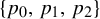
 $f,g$
are equivalent or combinatorially equivalent (or Thurston equivalent) if there exist orientation-preserving homeomorphisms
$f,g$
are equivalent or combinatorially equivalent (or Thurston equivalent) if there exist orientation-preserving homeomorphisms
 ${h_0,h_1:(\mathbb {C}, P_f)\rightarrow (\mathbb {C},P_g)}$
such that
${h_0,h_1:(\mathbb {C}, P_f)\rightarrow (\mathbb {C},P_g)}$
such that
 $h_0f=gh_1$
, and
$h_0f=gh_1$
, and
 $h_0$
and
$h_0$
and
 $h_1$
are homotopic relative to
$h_1$
are homotopic relative to
 $P_f$
. Thurston proved that a post-critically finite branched cover
$P_f$
. Thurston proved that a post-critically finite branched cover
 $\mathbb {C}\rightarrow \mathbb {C}$
is either equivalent to a polynomial or has a certain kind of topological obstruction [Reference Douady and Hubbard6]. Over the past decades, much work has been directed toward determining a holomorphic map to which an unobstructed branched cover
$\mathbb {C}\rightarrow \mathbb {C}$
is either equivalent to a polynomial or has a certain kind of topological obstruction [Reference Douady and Hubbard6]. Over the past decades, much work has been directed toward determining a holomorphic map to which an unobstructed branched cover
 $\mathbb {C}\to \mathbb {C}$
(or
$\mathbb {C}\to \mathbb {C}$
(or
 $S^2\to S^2$
) is equivalent [Reference Bartholdi and Dudko1–Reference Bonnot, Braverman and Yampolsky5, Reference Hubbard and Schleicher11, Reference Kelsey and Lodge12, Reference Nekrashevych14, Reference Nekrashevych15, Reference Rafi, Selinger and Yampolsky17–Reference Thurston19].
$S^2\to S^2$
) is equivalent [Reference Bartholdi and Dudko1–Reference Bonnot, Braverman and Yampolsky5, Reference Hubbard and Schleicher11, Reference Kelsey and Lodge12, Reference Nekrashevych14, Reference Nekrashevych15, Reference Rafi, Selinger and Yampolsky17–Reference Thurston19].
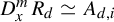
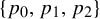
In the 1980s, Hubbard posed the twisted rabbit problem, which presented the challenge of classifying certain branched covers by the polynomial to which they were equivalent. The rabbit polynomial is the quadratic polynomial
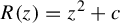 $R(z)=z^2+c$
, where
$R(z)=z^2+c$
, where
 $c\approx -0.122561+0.744862i$
for which the critical point 0 is 3-periodic. The post-critical set consists of three points:
$c\approx -0.122561+0.744862i$
for which the critical point 0 is 3-periodic. The post-critical set consists of three points:
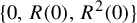 $\{0,R(0),R^2(0)\}$
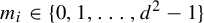
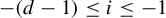
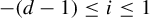
. Let x be a curve surrounding
$\{0,R(0),R^2(0)\}$
. Let x be a curve surrounding
 $R(0)$
and
$R(0)$
and
 $R^2(0)$
, and let
$R^2(0)$
, and let
 $D_x$
be the Dehn twist about x (see Figure 1). The composition
$D_x$
be the Dehn twist about x (see Figure 1). The composition
 $D_x^mR$
is a branched cover
$D_x^mR$
is a branched cover
 $\mathbb {C}\rightarrow \mathbb {C}$
, and by the Bernstein–Levy theorem [Reference Levy13] (also [Reference Hubbard10, Ch. 10]), it is equivalent to a polynomial. Hubbard’s twisted rabbit problem is as follows: for
$\mathbb {C}\rightarrow \mathbb {C}$
, and by the Bernstein–Levy theorem [Reference Levy13] (also [Reference Hubbard10, Ch. 10]), it is equivalent to a polynomial. Hubbard’s twisted rabbit problem is as follows: for
 $m \in \mathbb {Z}$
, find a function in terms of m that determines to which polynomial
$m \in \mathbb {Z}$
, find a function in terms of m that determines to which polynomial
 $D_x^mR$
is equivalent. After remaining open for nearly 25 years, Bartholdi and Nekrachevych solved the twisted rabbit problem in 2006 [Reference Bartholdi and Nekrashevych2].
$D_x^mR$
is equivalent. After remaining open for nearly 25 years, Bartholdi and Nekrachevych solved the twisted rabbit problem in 2006 [Reference Bartholdi and Nekrashevych2].
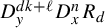
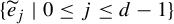
The Hubbard tree of the rabbit polynomial along with the simple closed curves x, y, and z.

Belk, Lanier, Margalit, and the second author solved a generalization of the twisted rabbit problem in which they compose quadratic polynomials where the critical point is n-periodic with powers of an analogous Dehn twist for
 $n\geq 3$
[Reference Belk, Lanier, Margalit and Winarski3]. Recently, Lanier and the second author extended their work to unicritical cubic polynomials (with any number of post-critical points).
$n\geq 3$
[Reference Belk, Lanier, Margalit and Winarski3]. Recently, Lanier and the second author extended their work to unicritical cubic polynomials (with any number of post-critical points).
1.1 The degree-d twisted rabbit problem
In this paper, we generalize Hubbard’s twisted rabbit problem to higher degree analogs of the rabbit polynomial. That is: for each
 $d\geq 2$
, there is a unicritical polynomial
$d\geq 2$
, there is a unicritical polynomial
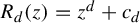 $R_d(z)=z^d+c_d$
that naturally generalizes the rabbit polynomial. The critical point
$R_d(z)=z^d+c_d$
that naturally generalizes the rabbit polynomial. The critical point
 $0$
is 3-periodic, as in the quadratic case. Let
$0$
is 3-periodic, as in the quadratic case. Let
 $x_d$
be the curve that is homotopic to the boundary of a neighborhood of the straight line segment between
$x_d$
be the curve that is homotopic to the boundary of a neighborhood of the straight line segment between
 $R_d(0)$
and
$R_d(0)$
and
 $R_d^2(0)$
. In Theorem 1.1, we describe a function that determines to which polynomial
$R_d^2(0)$
. In Theorem 1.1, we describe a function that determines to which polynomial
 $D_{x_d}^mR_d$
is equivalent in terms of m.
$D_{x_d}^mR_d$
is equivalent in terms of m.
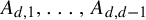
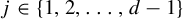
1.2 The polynomials
Before we state the solution to the degree-d twisted rabbit problem, we explain the notation we use for the polynomials that appear. For each degree d, there exist
 $d+1$
equivalence classes of polynomials that have a critical point that is 3-periodic. One of these is
$d+1$
equivalence classes of polynomials that have a critical point that is 3-periodic. One of these is
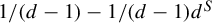
 $R_d$
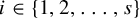
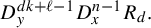
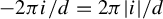
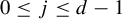
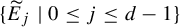
, the generalization of the rabbit polynomial (the degree-d rabbit); see Figure 2(a) for the Julia set when
$R_d$
, the generalization of the rabbit polynomial (the degree-d rabbit); see Figure 2(a) for the Julia set when
 $d=5$
. The complex conjugate of the rabbit polynomial is called the degree-d corabbit polynomial
$d=5$
. The complex conjugate of the rabbit polynomial is called the degree-d corabbit polynomial
 $\overline {R}_d$
, see Figure 2(b) for its Julia set when
$\overline {R}_d$
, see Figure 2(b) for its Julia set when
 $d=5$
. The remaining
$d=5$
. The remaining
 $d-1$
polynomials are all generalizations of the airplane polynomial. These remaining
$d-1$
polynomials are all generalizations of the airplane polynomial. These remaining
 $d-1$
polynomials have a Hubbard tree with two edges that meet at the critical point and can be indexed by the angle made by these two edges at the critical point with a fixed orientation. For
$d-1$
polynomials have a Hubbard tree with two edges that meet at the critical point and can be indexed by the angle made by these two edges at the critical point with a fixed orientation. For
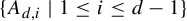
 $1 \leq i \leq d-1$
, we denote by
$1 \leq i \leq d-1$
, we denote by
 $A_{d,i}$
the degree-d generalization of the airplane for which this angle is
$A_{d,i}$
the degree-d generalization of the airplane for which this angle is
 ${2\pi i}/{d}$
; see Figures 2(c)–2(f) for the Julia sets of the four degree-d airplanes when
${2\pi i}/{d}$
; see Figures 2(c)–2(f) for the Julia sets of the four degree-d airplanes when
 $d=5$
.
$d=5$
.
The Julia sets and Hubbard trees for the unicritical polynomials of degree
 $5$
with 3-periodic critical point.
$5$
with 3-periodic critical point.

The solution to the original (quadratic) twisted rabbit problem depends on the 4-adic expansion of the power by which we twist. Similarly, the solution to the degree-d twisted rabbit problem will depend on the
 $d^2$
-adic expansion of the power by which we twist.
$d^2$
-adic expansion of the power by which we twist.
Any integer m has a
 $d^2$
-adic expansion of the form
$d^2$
-adic expansion of the form
 $m_sm_{s-1}m_{s-2}\cdots m_1$
if
$m_sm_{s-1}m_{s-2}\cdots m_1$
if
 ${m\geq 0}$
, or
${m\geq 0}$
, or
 $\overline {d^2-1}m_sm_{s-1}m_{s-2}\cdots m_1 $
if
$\overline {d^2-1}m_sm_{s-1}m_{s-2}\cdots m_1 $
if
 $m<0$
, with
$m<0$
, with
 $m_i \in \{0,1,\ldots ,d^2-1\}$
for all
$m_i \in \{0,1,\ldots ,d^2-1\}$
for all
 ${i \in \{1,2,\ldots ,s\}}$
. Let
${i \in \{1,2,\ldots ,s\}}$
. Let
 $\sigma _{d^2}(m)$
be the least value of s such that all digits of the
$\sigma _{d^2}(m)$
be the least value of s such that all digits of the
 $d^2$
-adic expansion of m to the left of
$d^2$
-adic expansion of m to the left of
 $m_s$
are repeating (that is, for all
$m_s$
are repeating (that is, for all
 $t>s$
,
$t>s$
,
 $m_t=0$
if
$m_t=0$
if
 $m\geq 0$
or
$m\geq 0$
or
 $m_t=d^2-1$
if
$m_t=d^2-1$
if
 $m<0$
).
$m<0$
).
Theorem 1.1. Let
 $R_d$
be the degree-d rabbit polynomial and
$R_d$
be the degree-d rabbit polynomial and
 $D_x$
the Dehn twist about the curve
$D_x$
the Dehn twist about the curve
 $x=x_d$
.
$x=x_d$
.
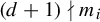
If
 $(d+1)| m_i$
for all
$(d+1)| m_i$
for all
 $i \in \{1,2,\ldots ,\sigma _{d^2}(m)\}$
, then
$i \in \{1,2,\ldots ,\sigma _{d^2}(m)\}$
, then
 $$ \begin{align*}D_x^mR_d \simeq \begin{cases} R_d &\text{if }m \geq 0,\\ \overline{R}_d&\text{if }m<0. \end{cases}\end{align*} $$
Otherwise, let i be the least index such that
 $m_i$
is not divisible by
$m_i$
is not divisible by
 $d+1$
. We may write
$d+1$
. We may write
 $m_i$
uniquely as
$m_i$
uniquely as
 $d\ell +n$
, where
$d\ell +n$
, where
 $\ell ,n \in \{0,1,\ldots ,d-1\}$
. Since
$\ell ,n \in \{0,1,\ldots ,d-1\}$
. Since
 $(d+1)\nmid m_i$
, we have that
$(d+1)\nmid m_i$
, we have that
 $\ell \neq n$
. Then,
$\ell \neq n$
. Then,
 $$ \begin{align*}D_x^mR_d \simeq \begin{cases} A_{d,n-\ell} &\text{if } n>\ell,\\ A_{d,d-(\ell-n)} &\text{if }n<\ell. \end{cases}\end{align*} $$
In particular, in the set
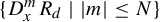 $\{D_x^mR_d\mid |m|\leq N\}$
, the airplane polynomials
$\{D_x^mR_d\mid |m|\leq N\}$
, the airplane polynomials
 $A_{d,1},\ldots , A_{d,d-1}$
occur with equal frequency. Moreover, as N tends to infinity, the probability that
$A_{d,1},\ldots , A_{d,d-1}$
occur with equal frequency. Moreover, as N tends to infinity, the probability that
 $D_x^mR_d$
(with
$D_x^mR_d$
(with
 $|m|\leq N$
) is equivalent to the rabbit or corabbit polynomial approaches zero.
$|m|\leq N$
) is equivalent to the rabbit or corabbit polynomial approaches zero.
Corollary 1.2. Fix a degree d greater than 1. For
 $S\geq 1$
, let
$S\geq 1$
, let
 $$ \begin{align*}\Sigma_S=\{m\in\mathbb{Z}\mid\sigma_{d^2}(m)\leq S\}.\end{align*} $$
With the uniform distribution on
 $\Sigma _S$
, the probability that for
$\Sigma _S$
, the probability that for
 $m \in \Sigma _S$
,
$m \in \Sigma _S$
,
 $D_x^mR_d$
is equivalent to a map in the collection
$D_x^mR_d$
is equivalent to a map in the collection
 $\{A_{d,i}\mid 1\leq i\leq d-1\}$
is given by
$\{A_{d,i}\mid 1\leq i\leq d-1\}$
is given by
 $1-{1}/{d^S}$
. In particular, for
$1-{1}/{d^S}$
. In particular, for
 $m \in \Sigma _S$
, we have the following.
$m \in \Sigma _S$
, we have the following.
-
• For any
 $i \in \{1,2,\ldots ,d-1\}$
, the probability that
$D_x^mR_d\simeq A_{d,i}$
is
${1}/({d-1}) - {1}/{(d-1)d^S}$
.
$i \in \{1,2,\ldots ,d-1\}$
, the probability that
$D_x^mR_d\simeq A_{d,i}$
is
${1}/({d-1}) - {1}/{(d-1)d^S}$
. -
• The probability that
$D_x^mR_d \simeq R_d$
is
${1}/{2d^S}$
. -
• The probability that
$D_x^mR_d \simeq \overline {R}_d$
is
${1}/{2d^S}$
.


Example 1.3. To make Theorem 1.1 concrete, we give the polynomials to which
 $D_x^mR_5$
is equivalent for
$D_x^mR_5$
is equivalent for
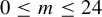 $0\leq m\leq 24$
in Table 1. We observe that
$0\leq m\leq 24$
in Table 1. We observe that
 $A_{5,1},\ldots , A_{5,4}$
each appear four times and
$A_{5,1},\ldots , A_{5,4}$
each appear four times and
 $R_d$
appears five times. The next m for which
$R_d$
appears five times. The next m for which
 $D_x^mR_5$
is equivalent to the rabbit is
$D_x^mR_5$
is equivalent to the rabbit is
 $m=150$
, which has 25-adic expansion
$m=150$
, which has 25-adic expansion
 $m_2m_1$
, with
$m_2m_1$
, with
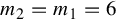 $m_2 = m_1 = 6$
. We also note that
$m_2 = m_1 = 6$
. We also note that
 $\overline {R}_5$
does not appear in the table because it only occurs when
$\overline {R}_5$
does not appear in the table because it only occurs when
 $m<0$
. For
$m<0$
. For
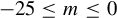 $-25\leq m\leq 0$
, the polynomial
$-25\leq m\leq 0$
, the polynomial
 $\overline {R}_d$
occurs when
$\overline {R}_d$
occurs when
 $m=-1,-7,-13,-19,-25$
.
$m=-1,-7,-13,-19,-25$
.
Base cases for
 $d=5$
.
$d=5$
.

1.3 Methods
We follow the strategy of Bartholdi and Nekrashevych [Reference Bartholdi and Nekrashevych2]: in §3, we find formulas that reduce
 $D_x^mR_d$
to
$D_x^mR_d$
to
 $R_d$
post-composed with one of a finite set of maps. Then, in §4, we determine a polynomial equivalent to each of these ‘base cases’ using the lifting algorithm of Belk, Lanier, Margalit, and the second author in [Reference Belk, Lanier, Margalit and Winarski3].
$R_d$
post-composed with one of a finite set of maps. Then, in §4, we determine a polynomial equivalent to each of these ‘base cases’ using the lifting algorithm of Belk, Lanier, Margalit, and the second author in [Reference Belk, Lanier, Margalit and Winarski3].
1.4 Other twisted rabbit problems
As mentioned above, the (quadradic) twisted rabbit problem remained open for over two decades. When Bartholdi and Nekrashevych solved the problem, it shifted the techniques used to study holomorphic dynamics. However, they gave more than just a solution to the problem that Hubbard originally posed: for instance, they gave an algorithm to determine the polynomial to which
 $gR_2$
was equivalent for any pure mapping class g. Their work opened up a world of possible generalizations: in this paper, we follow their lead by increasing the degree of the polynomial by which we twist. Belk, Lanier, Margalit, and the second author generalize the (quadratic) twisted rabbit problem by increasing the size of the post-critical set. In concurrent work of Lanier and the second author, they solve several of these problems for the cubic rabbit polynomial. In particular, they give a closed-form solution to
$gR_2$
was equivalent for any pure mapping class g. Their work opened up a world of possible generalizations: in this paper, we follow their lead by increasing the degree of the polynomial by which we twist. Belk, Lanier, Margalit, and the second author generalize the (quadratic) twisted rabbit problem by increasing the size of the post-critical set. In concurrent work of Lanier and the second author, they solve several of these problems for the cubic rabbit polynomial. In particular, they give a closed-form solution to
 $D_x^mR_3$
that agrees with our solution in that case. They also generalize this case to give a closed-form solution to determine the equivalence class of
$D_x^mR_3$
that agrees with our solution in that case. They also generalize this case to give a closed-form solution to determine the equivalence class of
 $D_x^mR_{3,n}$
, where
$D_x^mR_{3,n}$
, where
 $R_{3,n}$
is a specific cubic polynomial with n post-critical points that is a natural generalization of
$R_{3,n}$
is a specific cubic polynomial with n post-critical points that is a natural generalization of
 $R_3$
. By pairing our paper with theirs, we have a 2-parameter family of generalizations of the twisted rabbit problem: by varying both the degree d and the number of post-critical points. In this paper, we prove that we can obtain any equivalence class of a degree d-unicritical polynomial with a 3-periodic critical point by twisting the degree d rabbit polynomial by a power of
$R_3$
. By pairing our paper with theirs, we have a 2-parameter family of generalizations of the twisted rabbit problem: by varying both the degree d and the number of post-critical points. In this paper, we prove that we can obtain any equivalence class of a degree d-unicritical polynomial with a 3-periodic critical point by twisting the degree d rabbit polynomial by a power of
 $D_x$
. Lanier and the second author show that the same is not true when the critical point has period greater than 3 (at least in the cubic case). Further investigation into this 2-parameter family of twisted rabbit problems may reveal deeper structure or patterns within the set of unicritical polynomials with periodic critical point.
$D_x$
. Lanier and the second author show that the same is not true when the critical point has period greater than 3 (at least in the cubic case). Further investigation into this 2-parameter family of twisted rabbit problems may reveal deeper structure or patterns within the set of unicritical polynomials with periodic critical point.
2 Hubbard trees and degree-d polynomials
Throughout this paper, we rely heavily on the established theory of Hubbard trees [Reference Douady and Hubbard7, Reference Douady and Hubbard8]. We will use a modification of Poirier’s conditions for Hubbard trees to allow us to define (topological) Hubbard trees for unobstructed branched covers
 $\mathbb {C}\to \mathbb {C}$
[Reference Douady and Hubbard6, Reference Poirier16].
$\mathbb {C}\to \mathbb {C}$
[Reference Douady and Hubbard6, Reference Poirier16].
2.1 Hubbard trees
Let
 $f:\mathbb {C}\rightarrow \mathbb {C}$
be a post-critically finite branched cover with post-critical set
$f:\mathbb {C}\rightarrow \mathbb {C}$
be a post-critically finite branched cover with post-critical set
 $P_f$
. For our purposes, a tree T is a finite graph with no cycles, embedded in
$P_f$
. For our purposes, a tree T is a finite graph with no cycles, embedded in
 $\mathbb {C}$
such that:
$\mathbb {C}$
such that:
-
(1)
$P_f$
is contained in the vertex set of T and -
(2) all leaves of T are in
$P_f$
.


The preimage
 $f^{-1}(T)$
does not, in general, satisfy the definition of a tree given above. The lift of a tree T, denoted
$f^{-1}(T)$
does not, in general, satisfy the definition of a tree given above. The lift of a tree T, denoted
 $\widetilde {T}$
, is the hull of
$\widetilde {T}$
, is the hull of
 $f^{-1}(T)$
relative to
$f^{-1}(T)$
relative to
 $P_f$
. That is, any edge of
$P_f$
. That is, any edge of
 $f^{-1}(T)$
that is not contained in a path between a pair of points in
$f^{-1}(T)$
that is not contained in a path between a pair of points in
 $P_f$
is contracted to a point. Thus,
$P_f$
is contracted to a point. Thus,
 $\widetilde {T}$
is a tree. We say two trees T and
$\widetilde {T}$
is a tree. We say two trees T and
 $T'$
are isomorphic if they are homeomorphic as topological spaces.
$T'$
are isomorphic if they are homeomorphic as topological spaces.
Let f be a polynomial of degree
 $d\geq 2$
. Let
$d\geq 2$
. Let
 $P_f$
be the post-critical set for f. The Hubbard tree
$P_f$
be the post-critical set for f. The Hubbard tree
 $H_f$
for f is a subset of
$H_f$
for f is a subset of
 $\mathbb {C}$
comprising regulated arcs of the filled Julia set of f that connect pairs of points of
$\mathbb {C}$
comprising regulated arcs of the filled Julia set of f that connect pairs of points of
 $P_f$
(see [Reference Poirier16] or [Reference Hubbard10]). An important feature of the Hubbard tree of f is that it is invariant under f, that is,
$P_f$
(see [Reference Poirier16] or [Reference Hubbard10]). An important feature of the Hubbard tree of f is that it is invariant under f, that is,
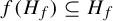 $f(H_f)\subseteq H_f$
. Likewise, it is also true that
$f(H_f)\subseteq H_f$
. Likewise, it is also true that
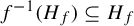 $f^{-1}(H_f)\subseteq H_f$
and that
$f^{-1}(H_f)\subseteq H_f$
and that
 $H_f$
is isotopic to
$H_f$
is isotopic to
 $\widetilde {H}_f$
.
$\widetilde {H}_f$
.
Let g be a branched cover
 $\mathbb {C}\to \mathbb {C}$
that is equivalent to f. Then, we can define the (topological) Hubbard tree for g, denoted
$\mathbb {C}\to \mathbb {C}$
that is equivalent to f. Then, we can define the (topological) Hubbard tree for g, denoted
 $H_g$
, as the pullback of
$H_g$
, as the pullback of
 $H_f$
under the equivalence between f and g. In this case, the abstract trees for
$H_f$
under the equivalence between f and g. In this case, the abstract trees for
 $H_f$
and
$H_f$
and
 $H_g$
are isomorphic.
$H_g$
are isomorphic.
Angle assignments. The combinatorial structure of a Hubbard tree is not sufficient to distinguish the combinatorial equivalence class of a branched cover
 $\mathbb {C}\to \mathbb {C}$
. That is, there are inequivalent polynomials that have isomorphic Hubbard trees. There is additional information that one can provide to distinguish post-critically finite branched covers. Following Poirier (see [Reference Poirier16]), we use an invariant angle assignment, which we define as follows. Because we think of a (Hubbard) tree as a subset of
$\mathbb {C}\to \mathbb {C}$
. That is, there are inequivalent polynomials that have isomorphic Hubbard trees. There is additional information that one can provide to distinguish post-critically finite branched covers. Following Poirier (see [Reference Poirier16]), we use an invariant angle assignment, which we define as follows. Because we think of a (Hubbard) tree as a subset of
 $\mathbb {C}$
, the edges that meet at any vertex have an associated cyclic order. An angle assignment for a vertex v is a set of angle measures between each pair of (not necessarily distinct) edges that have endpoint v and are adjacent in the cyclic order around v such that the measures of the angles sum to
$\mathbb {C}$
, the edges that meet at any vertex have an associated cyclic order. An angle assignment for a vertex v is a set of angle measures between each pair of (not necessarily distinct) edges that have endpoint v and are adjacent in the cyclic order around v such that the measures of the angles sum to
 $2\pi $
. An angle assignment for a tree T is the union of angle assignments at each of the vertices of T.
$2\pi $
. An angle assignment for a tree T is the union of angle assignments at each of the vertices of T.
The tree lift
 $\widetilde {T}$
inherits an angle assignment from T, as follows. Let
$\widetilde {T}$
inherits an angle assignment from T, as follows. Let
 $\angle $
be an angle of T adjacent to the vertex
$\angle $
be an angle of T adjacent to the vertex
 $v\in T$
with measure
$v\in T$
with measure
 $|\angle |$
. Let
$|\angle |$
. Let
 $\widetilde {v}\in f^{-1}(v)$
, and let
$\widetilde {v}\in f^{-1}(v)$
, and let
 $\nu (\widetilde {v})$
denote the local degree of
$\nu (\widetilde {v})$
denote the local degree of
 $\widetilde {v}$
under f. There exists a preimage of the angle
$\widetilde {v}$
under f. There exists a preimage of the angle
 $\angle $
at
$\angle $
at
 $\widetilde {v}$
, denoted
$\widetilde {v}$
, denoted
 $\widetilde {\angle }$
. Assign the measure of
$\widetilde {\angle }$
. Assign the measure of
 ${|\angle |}/{\nu (\widetilde {v})}$
to the angle
${|\angle |}/{\nu (\widetilde {v})}$
to the angle
 $\widetilde {\angle }$
. By applying this process to each angle in T, we define an angle assignment on
$\widetilde {\angle }$
. By applying this process to each angle in T, we define an angle assignment on
 $f^{-1}(T)$
. To define an angle assignment on
$f^{-1}(T)$
. To define an angle assignment on
 $\widetilde {T}$
, consider any edge e in
$\widetilde {T}$
, consider any edge e in
 $f^{-1}(T)$
that is contracted to a point of
$f^{-1}(T)$
that is contracted to a point of
 $\widetilde {T}$
. The edge e is the side of two angles
$\widetilde {T}$
. The edge e is the side of two angles
 $\angle _1$
and
$\angle _1$
and
 $\angle _2$
. When e is contracted to a point of
$\angle _2$
. When e is contracted to a point of
 $\widetilde {T}$
, the two angles
$\widetilde {T}$
, the two angles
 $\angle _1$
and
$\angle _1$
and
 $\angle _2$
are replaced with a new angle
$\angle _2$
are replaced with a new angle
 $\angle '$
. Assign the measure of
$\angle '$
. Assign the measure of
 $\angle '$
to be
$\angle '$
to be
 $|\angle _1|+|\angle _2|$
. We say an angle assignment on T is invariant if:
$|\angle _1|+|\angle _2|$
. We say an angle assignment on T is invariant if:
-
(1) T is isotopic to
$\widetilde {T}$
and -
(2) each angle of T has the same measure as the corresponding angle (under the isotopy) of
$\widetilde {T}$
.


Given a branched cover
 $f:\mathbb {C}\to \mathbb {C}$
, it follows from the work of Douady and Hubbard [Reference Douady and Hubbard7, Reference Douady and Hubbard8] or Poirier [Reference Poirier16] that a Hubbard tree
$f:\mathbb {C}\to \mathbb {C}$
, it follows from the work of Douady and Hubbard [Reference Douady and Hubbard7, Reference Douady and Hubbard8] or Poirier [Reference Poirier16] that a Hubbard tree
 $H_f$
, an invariant angle assignment on
$H_f$
, an invariant angle assignment on
 $H_f$
, and the restriction of f to
$H_f$
, and the restriction of f to
 $\widetilde {H}_f$
suffice to determine the equivalence class of f.
$\widetilde {H}_f$
suffice to determine the equivalence class of f.
2.2 The degree-d polynomials with a 3-periodic critical cycle
In this section, we describe the Hubbard trees for all unicritical polynomials of degree d with a
 $3$
-periodic critical point. We first count the equivalence classes of such polynomials.
$3$
-periodic critical point. We first count the equivalence classes of such polynomials.
Counting parameter rays. Every unicritical polynomial of degree d is affine conjugate to
 $z^d+c$
for some
$z^d+c$
for some
 $c \in \mathbb {C}$
. There exist exactly
$c \in \mathbb {C}$
. There exist exactly
 $d^2-1$
polynomials in this family that have a critical cycle of period
$d^2-1$
polynomials in this family that have a critical cycle of period
 $3$
. Indeed, this may be seen by counting angles of parameter rays in the Mandelbrot set. The parameter rays that land on a hyperbolic component of the Mandelbrot set that contains a polynomial with a critical cycle of period dividing 3 exactly comprise the set of parameter rays with angles in
$3$
. Indeed, this may be seen by counting angles of parameter rays in the Mandelbrot set. The parameter rays that land on a hyperbolic component of the Mandelbrot set that contains a polynomial with a critical cycle of period dividing 3 exactly comprise the set of parameter rays with angles in
 $\{{i}/{d^3-1}\mid i \in \{0,1,2,\ldots ,d^3-2\}\}$
. Among such rays, the rays at the angles
$\{{i}/{d^3-1}\mid i \in \{0,1,2,\ldots ,d^3-2\}\}$
. Among such rays, the rays at the angles
 $0, {1}/({d-1}),{2}/({d-1}),\ldots ,({d-2})/({d-1})$
land on the unique hyperbolic component of period 1. Of the remaining
$0, {1}/({d-1}),{2}/({d-1}),\ldots ,({d-2})/({d-1})$
land on the unique hyperbolic component of period 1. Of the remaining
 $d^3-d $
rays, groups of d rays each land on the same hyperbolic component. Thus, there are
$d^3-d $
rays, groups of d rays each land on the same hyperbolic component. Thus, there are
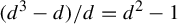 $(d^3-d)/d=d^2-1$
hyperbolic components that contain unicritical polynomials with critical cycle of period
$(d^3-d)/d=d^2-1$
hyperbolic components that contain unicritical polynomials with critical cycle of period
 $3$
. However, the affine conjugacy class (and therefore the equivalence class) of each polynomial
$3$
. However, the affine conjugacy class (and therefore the equivalence class) of each polynomial
 $z^d+c$
consists of the
$z^d+c$
consists of the
 $d-1$
polynomials
$d-1$
polynomials
 $z^d + \omega ^j c$
, where
$z^d + \omega ^j c$
, where
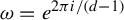 $\omega = e^{{2 \pi i}/({d-1})}$
and
$\omega = e^{{2 \pi i}/({d-1})}$
and
 $j \in \{1,2,\ldots ,d-1\}$
. Thus, there are exactly
$j \in \{1,2,\ldots ,d-1\}$
. Thus, there are exactly
 $d+1$
equivalence classes of unicritical polynomials that have a critical cycle of exact period
$d+1$
equivalence classes of unicritical polynomials that have a critical cycle of exact period
 $3$
.
$3$
.
Alternatively, we observe that every polynomial of the form
 $z^d+c$
with
$z^d+c$
with
 $c\neq 0$
is conjugate to the polynomial
$c\neq 0$
is conjugate to the polynomial
 $p_\unicode{x3bb} (z) = \unicode{x3bb} (1+{z}/{d})^d$
, where
$p_\unicode{x3bb} (z) = \unicode{x3bb} (1+{z}/{d})^d$
, where
 $\unicode{x3bb} = dc^{d-1}$
. In the polynomial family
$\unicode{x3bb} = dc^{d-1}$
. In the polynomial family
 $\{p_\unicode{x3bb} \}$
, the polynomials
$\{p_\unicode{x3bb} \}$
, the polynomials
 $p_{\unicode{x3bb} _1}$
and
$p_{\unicode{x3bb} _1}$
and
 $p_{\unicode{x3bb} _2}$
are conjugate if and only if
$p_{\unicode{x3bb} _2}$
are conjugate if and only if
 $\unicode{x3bb} _1 = \unicode{x3bb} _2$
. In this family, there are exactly
$\unicode{x3bb} _1 = \unicode{x3bb} _2$
. In this family, there are exactly
 $d+1$
distinct solutions to the equation
$d+1$
distinct solutions to the equation
 $p_\unicode{x3bb} ^{\circ 3}(0) = 0.$
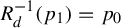
2.2.1 Hubbard trees of polynomials with three critical points
Let f be a unicritical polynomial of degree d with a 3-periodic critical point. Let
 $p_0$
be the critical point of f, let
$p_0$
be the critical point of f, let
 $p_1=f(p_0)$
be the critical value, and let
$p_1=f(p_0)$
be the critical value, and let
 $p_2=f^2(p_0)$
.
$p_2=f^2(p_0)$
.
The
 $d+1$
equivalence classes of degree d polynomials that have a critical point of period 3 can be distinguished by their Hubbard trees and an invariant angle assignment. There are only two combinatorial structures for (Hubbard) trees with three post-critical points:
$d+1$
equivalence classes of degree d polynomials that have a critical point of period 3 can be distinguished by their Hubbard trees and an invariant angle assignment. There are only two combinatorial structures for (Hubbard) trees with three post-critical points:
-
(1) a tripod, that is, a graph where
$\{p_0,p_1,p_2\}$
are all leaves and there is an unmarked trivalent vertex or -
(2) a path of length 2 (two of the post-critical points are leaves).
2.2.2 The rabbit
$R_d$
and corabbit
$\overline {R}_d$


The rabbit polynomial
 $R_d$
and corabbit polynomial
$R_d$
and corabbit polynomial
 $\overline {R}_d$
are the two polynomials (up to equivalence) that have a tripod as their Hubbard tree. Both polynomials cyclically permute edges. Therefore, the only possible invariant angle assignment is
$\overline {R}_d$
are the two polynomials (up to equivalence) that have a tripod as their Hubbard tree. Both polynomials cyclically permute edges. Therefore, the only possible invariant angle assignment is
 ${2\pi }/{3}$
at all angles, in both cases. They can be distinguished, however, because
${2\pi }/{3}$
at all angles, in both cases. They can be distinguished, however, because
 $R_d$
rotates the edges of its Hubbard tree counterclockwise and
$R_d$
rotates the edges of its Hubbard tree counterclockwise and
 $\overline {R}_d$
rotates the edges of its Hubbard tree clockwise. Because a polynomial is determined by its Hubbard tree, the invariant angle assignment, and the action of the map on the edges of its Hubbard tree, we may take this to be the definition of
$\overline {R}_d$
rotates the edges of its Hubbard tree clockwise. Because a polynomial is determined by its Hubbard tree, the invariant angle assignment, and the action of the map on the edges of its Hubbard tree, we may take this to be the definition of
 $R_d$
and
$R_d$
and
 $\overline {R}_d$
. Where
$\overline {R}_d$
. Where
 $d=5$
, the Hubbard tree for
$d=5$
, the Hubbard tree for
 $R_5$
is shown as a subset of the filled Julia set in Figure 2(a) and the Hubbard tree for
$R_5$
is shown as a subset of the filled Julia set in Figure 2(a) and the Hubbard tree for
 $\overline {R}_5$
is a subset of the filled Julia set in Figure 2(b).
$\overline {R}_5$
is a subset of the filled Julia set in Figure 2(b).
2.2.3 The airplanes
$A_{d,i}$

The remaining
 $d-1$
equivalence classes of polynomials have Hubbard trees that are paths of length 2. Moreover, the vertex of valence 2 must be
$d-1$
equivalence classes of polynomials have Hubbard trees that are paths of length 2. Moreover, the vertex of valence 2 must be
 $p_0$
because the critical point is the only point for which f maps a neighborhood d-to-1 to its image. The polynomials are distinguished by the invariant angle assignment on their Hubbard tree. For any
$p_0$
because the critical point is the only point for which f maps a neighborhood d-to-1 to its image. The polynomials are distinguished by the invariant angle assignment on their Hubbard tree. For any
 $i \in \{1,2,\ldots ,d-1\}$
, there is a polynomial such that
$i \in \{1,2,\ldots ,d-1\}$
, there is a polynomial such that
 $\angle p_1p_0p_2$
has an invariant angle assignment of
$\angle p_1p_0p_2$
has an invariant angle assignment of
 ${2\pi i}/{d}$
. Define
${2\pi i}/{d}$
. Define
 $A_{d,i}$
to be the polynomial where
$A_{d,i}$
to be the polynomial where
 $\angle p_1p_0p_2$
is
$\angle p_1p_0p_2$
is
 ${2\pi i}/{d}$
. Figures 2(c)–2(f) show the filled Julia sets and Hubbard trees (with angles) for
${2\pi i}/{d}$
. Figures 2(c)–2(f) show the filled Julia sets and Hubbard trees (with angles) for
 $A_{5,1}$
through
$A_{5,1}$
through
 $A_{5,4}$
, respectively.
$A_{5,4}$
, respectively.
3 Reduction formulas
We prove Theorem 1.1 in two steps, following the original proof of Bartholdi and Nekraschevych. In Lemma 3.2, we give an algorithm that determines a map to which
 $D_{x_d}^mR_d$
is equivalent and that either belongs to a finite set (of base cases) or is of the form
$D_{x_d}^mR_d$
is equivalent and that either belongs to a finite set (of base cases) or is of the form
 $D^k_{x_d}R_d$
, where
$D^k_{x_d}R_d$
, where
 $k\leq m$
. In the next section, we find a Hubbard tree for each of the base cases.
$k\leq m$
. In the next section, we find a Hubbard tree for each of the base cases.
3.1 Lifting
Let
 $P_d$
be the post-critical set of
$P_d$
be the post-critical set of
 $R_d$
. A homeomorphism
$R_d$
. A homeomorphism
 $h:(\mathbb {C},P_d)\rightarrow (\mathbb {C},P_d)$
is said to be liftable under
$h:(\mathbb {C},P_d)\rightarrow (\mathbb {C},P_d)$
is said to be liftable under
 $R_d$
if there exists a homeomorphism
$R_d$
if there exists a homeomorphism
 $\widetilde {h}:(\mathbb {C},P_d)\rightarrow (\mathbb {C},P_d)$
such that
$\widetilde {h}:(\mathbb {C},P_d)\rightarrow (\mathbb {C},P_d)$
such that
 $R_d\widetilde {h}=hR_d$
. In this case,
$R_d\widetilde {h}=hR_d$
. In this case,
 $hR_d$
is equivalent to
$hR_d$
is equivalent to
 $\widetilde {h}R_d$
. We use the notation
$\widetilde {h}R_d$
. We use the notation
to describe the (directional) equivalence between
 $hR_d$
and
$hR_d$
and
 $\widetilde {h}R_d$
.
$\widetilde {h}R_d$
.
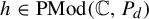
The isotopy classes of homeomorphisms that lift under
 $R_d$
form a finite index subgroup of
$R_d$
form a finite index subgroup of
 $\operatorname {\mathrm {PMod}}(\mathbb {C},P_d)$
called the liftable mapping class group
$\operatorname {\mathrm {PMod}}(\mathbb {C},P_d)$
called the liftable mapping class group
 $\operatorname {\mathrm {LMod}}(\mathbb {C},P_d)$
. As described above, there is a homomorphism
$\operatorname {\mathrm {LMod}}(\mathbb {C},P_d)$
. As described above, there is a homomorphism
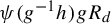
 $\psi : \operatorname {\mathrm {LMod}}(\mathbb {C},P_d)\to \operatorname {\mathrm {PMod}}(\mathbb {C},P_d)$
defined for
$\psi : \operatorname {\mathrm {LMod}}(\mathbb {C},P_d)\to \operatorname {\mathrm {PMod}}(\mathbb {C},P_d)$
defined for
 $h\in \operatorname {\mathrm {LMod}}(\mathbb {C},P_d)$
as
$h\in \operatorname {\mathrm {LMod}}(\mathbb {C},P_d)$
as
 $\psi (h)=\widetilde {h}$
.
$\psi (h)=\widetilde {h}$
.
Following Bartholdi and Nekrashevych, we use
 $\psi $
to define a version of lifting for any
$\psi $
to define a version of lifting for any
 $h\in \operatorname {\mathrm {PMod}}(\mathbb {C},P_d)$
. For any
$h\in \operatorname {\mathrm {PMod}}(\mathbb {C},P_d)$
. For any
 $h\in \operatorname {\mathrm {PMod}}(\mathbb {C},P_d)$
, there exists
$h\in \operatorname {\mathrm {PMod}}(\mathbb {C},P_d)$
, there exists
 $g\in \operatorname {\mathrm {PMod}}(\mathbb {C},P_d)$
such that
$g\in \operatorname {\mathrm {PMod}}(\mathbb {C},P_d)$
such that
 $g^{-1}h\in \operatorname {\mathrm {LMod}}(\mathbb {C},P_d)$
. Then,
$g^{-1}h\in \operatorname {\mathrm {LMod}}(\mathbb {C},P_d)$
. Then,
 $g^{-1}hR_d$
is equivalent to
$g^{-1}hR_d$
is equivalent to
 $\psi (g^{-1}h)R_d$
. Moreover,
$\psi (g^{-1}h)R_d$
. Moreover,
 $hR_d$
is equivalent to
$hR_d$
is equivalent to
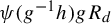 $\psi (g^{-1}h)gR_d$
[Reference Belk, Lanier, Margalit and Winarski3, Lemma 5.1]. We use the notation
$\psi (g^{-1}h)gR_d$
[Reference Belk, Lanier, Margalit and Winarski3, Lemma 5.1]. We use the notation
to denote the equivalence between
 $hR_d$
and
$hR_d$
and
 $\psi (g^{-1}h)gR_d$
obtained by lifting
$\psi (g^{-1}h)gR_d$
obtained by lifting
 $g^{-1}h$
under
$g^{-1}h$
under
 $R_d$
. In particular, the superscript g indicates which coset representative of
$R_d$
. In particular, the superscript g indicates which coset representative of
 $h\operatorname {\mathrm {LMod}}(\mathbb {C},P_d)$
we choose. If
$h\operatorname {\mathrm {LMod}}(\mathbb {C},P_d)$
we choose. If
 $h\in \operatorname {\mathrm {LMod}}(\mathbb {C},P_d)$
, the notation
$h\in \operatorname {\mathrm {LMod}}(\mathbb {C},P_d)$
, the notation ![]() is a special case of the notation
is a special case of the notation
where g is the identity, which we suppress.
3.2 Branch cuts
Let
 $f:\mathbb {C}\rightarrow \mathbb {C}$
be a post-critically finite branched cover of degree
$f:\mathbb {C}\rightarrow \mathbb {C}$
be a post-critically finite branched cover of degree
 $d\geq 2$
. A branch cut B is a union of arcs such that:
$d\geq 2$
. A branch cut B is a union of arcs such that:
-
• each endpoint of each arc in B is a critical value of f (possibly infinity);
-
• each critical value of f is an endpoint of an arc of B; and
-
• the complement of
$f^{-1}(B)$
in
$\mathbb {C}$
consists of d components.


If f is unicritical, B can be chosen to be a single arc b joining the unique critical value to infinity. A special branch cut for f is a branch cut such that all points in the post-critical set
 $P_f$
for f are contained in the closure of a single component of
$P_f$
for f are contained in the closure of a single component of
 $\mathbb {C} \setminus f^{-1}(b)$
.
$\mathbb {C} \setminus f^{-1}(b)$
.
3.3 Intersections with a branch cut
Let
 $\gamma $
be an arc in
$\gamma $
be an arc in
 $(\mathbb {C},P_f)$
with endpoints in
$(\mathbb {C},P_f)$
with endpoints in
 $P_f$
and let b be a branch cut for f. The preimage
$P_f$
and let b be a branch cut for f. The preimage
 $f^{-1}(\gamma )$
intersects the preimage
$f^{-1}(\gamma )$
intersects the preimage
 $f^{-1}(b)$
at
$f^{-1}(b)$
at
 $d|\gamma \cap b|$
points. Moreover, if we assign an orientation to b and
$d|\gamma \cap b|$
points. Moreover, if we assign an orientation to b and
 $\gamma $
, the points of intersection
$\gamma $
, the points of intersection
 $\gamma \cap b$
will inherit an orientation. The orientation of each point of
$\gamma \cap b$
will inherit an orientation. The orientation of each point of
 $\gamma \cap b$
will lift to an orientation of the corresponding d preimages of
$\gamma \cap b$
will lift to an orientation of the corresponding d preimages of
 $f^{-1}(\gamma )$
. The geometric intersection of
$f^{-1}(\gamma )$
. The geometric intersection of
 $\gamma $
and b is the minimum of
$\gamma $
and b is the minimum of
 $|\gamma \cap b|$
over all arcs homotopic to
$|\gamma \cap b|$
over all arcs homotopic to
 $\gamma $
. The algebraic intersection of
$\gamma $
. The algebraic intersection of
 $\gamma $
and b is the sum of the signed (from the orientation) intersections of the homotopy class representative of
$\gamma $
and b is the sum of the signed (from the orientation) intersections of the homotopy class representative of
 $\gamma $
that realizes the algebraic intersection.
$\gamma $
that realizes the algebraic intersection.
3.4 Defining arcs
Let c be a simple closed curve that bounds a disk that contains two points
 $p,q$
in
$p,q$
in
 $P_f$
. Then, c is homotopic to the boundary of a neighborhood of a simple arc
$P_f$
. Then, c is homotopic to the boundary of a neighborhood of a simple arc
 $\gamma _c$
with endpoints at p and q. We call
$\gamma _c$
with endpoints at p and q. We call
 $\gamma _c$
the defining arc of c.
$\gamma _c$
the defining arc of c.
A simple closed curve in
 $\mathbb {C} \setminus P_f$
is called trivial if it is homotopic to a point relative to
$\mathbb {C} \setminus P_f$
is called trivial if it is homotopic to a point relative to
 $P_f$
or bounds a single point of
$P_f$
or bounds a single point of
 $P_f$
. The next lemma gives a condition for when the preimage of a (non-trivial) curve is trivial.
$P_f$
. The next lemma gives a condition for when the preimage of a (non-trivial) curve is trivial.
Lemma 3.1. Let
 $f:\mathbb {C}\to \mathbb {C}$
be a post-critically finite branched cover of degree d and let b be a special branch cut for f. The complement of
$f:\mathbb {C}\to \mathbb {C}$
be a post-critically finite branched cover of degree d and let b be a special branch cut for f. The complement of
 $f^{-1}(b)$
in
$f^{-1}(b)$
in
 $\mathbb {C}$
consists of d (open) components. Label these components counterclockwise as
$\mathbb {C}$
consists of d (open) components. Label these components counterclockwise as
 $\Gamma _0,\ldots , \Gamma _{d-1}$
, where such
$\Gamma _0,\ldots , \Gamma _{d-1}$
, where such
 $\Gamma _0$
is the component such that its closure contains the -critical set.
$\Gamma _0$
is the component such that its closure contains the -critical set.
Let c be a curve in
 $(\mathbb {C},P_f)$
that bounds a disk containing two points in
$(\mathbb {C},P_f)$
that bounds a disk containing two points in
 $P_f$
such that neither point is the critical value. Let
$P_f$
such that neither point is the critical value. Let
 $\gamma _c$
be the defining arc of c. Suppose the algebraic intersection of
$\gamma _c$
be the defining arc of c. Suppose the algebraic intersection of
 $\gamma _c$
and b is i. Then, for each
$\gamma _c$
and b is i. Then, for each
 $0\leq j\leq d-1$
, there is a path lift of
$0\leq j\leq d-1$
, there is a path lift of
 $\gamma _c$
such that the endpoints of the path lift are in
$\gamma _c$
such that the endpoints of the path lift are in
 $\Gamma _j$
and
$\Gamma _j$
and
 $\Gamma _{(j-|i|)\mod d}$
. In particular, each component of
$\Gamma _{(j-|i|)\mod d}$
. In particular, each component of
 $f^{-1}(c)$
is trivial if and only if
$f^{-1}(c)$
is trivial if and only if
 $d\nmid i$
.
$d\nmid i$
.
Proof. For the first statement, induct on i.
The defining arc of each connected component of
 $f^{-1}(c)$
is a path lift of
$f^{-1}(c)$
is a path lift of
 $\gamma _c$
. We note that a lift of
$\gamma _c$
. We note that a lift of
 $\gamma _c$
is the defining arc of a non-trivial curve if and only if both endpoints are in
$\gamma _c$
is the defining arc of a non-trivial curve if and only if both endpoints are in
 $P_f\subset \Gamma _0$
. Moreover, the endpoints of a lift of
$P_f\subset \Gamma _0$
. Moreover, the endpoints of a lift of
 $\gamma _c$
are in the same component
$\gamma _c$
are in the same component
 $\Gamma _j$
if and only if
$\Gamma _j$
if and only if
 $d\mid i$
.
$d\mid i$
.
Lemma 3.2 is the key step that allows us to write
 $D_{x_d}^mR_d$
as a map with a lower power than m. Let
$D_{x_d}^mR_d$
as a map with a lower power than m. Let
 $x=x_d$
,
$x=x_d$
,
 $y=y_d$
, and
$y=y_d$
, and
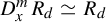
 $z=z_d$
be the curves in Figure 1.
$z=z_d$
be the curves in Figure 1.
Let c be a simple closed curve in
 $(\mathbb {C},R_d)$
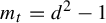
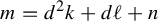
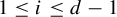
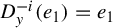
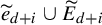
. Recall that the Dehn twist about c is trivial if and only if c is trivial. For example, in Figure 3, we illustrate the curve
$(\mathbb {C},R_d)$
. Recall that the Dehn twist about c is trivial if and only if c is trivial. For example, in Figure 3, we illustrate the curve
 $D_y^{-2}(z)$
and its lift under
$D_y^{-2}(z)$
and its lift under
 $R_5$
. By Lemma 3.1, all components of
$R_5$
. By Lemma 3.1, all components of
 $R_5^{-1}(D_y^{-2}(z))$
are trivial since
$R_5^{-1}(D_y^{-2}(z))$
are trivial since
 $5 \nmid -2$
; therefore, any lift of the
$5 \nmid -2$
; therefore, any lift of the
 $D_{D_y^{-2}(z)}$
under
$D_{D_y^{-2}(z)}$
under
 $R_5$
is trivial.
$R_5$
is trivial.
(a) The simple closed curves y and z. (b) The simple closed curve
 $D_y^{-2}(z)$
. (c) The preimage of
$D_y^{-2}(z)$
. (c) The preimage of
 $D_y^{-2}(z)$
under
$D_y^{-2}(z)$
under
 $R_d$
when
$R_d$
when
 $d=5$
. All components of the preimage are peripheral.
$d=5$
. All components of the preimage are peripheral.

Lemma 3.2. Let
 $m \in \mathbb {Z}$
,
$m \in \mathbb {Z}$
,
 $m = d^2k+d\ell +n$
with
$m = d^2k+d\ell +n$
with
 $k \in \mathbb {Z},$
and
$k \in \mathbb {Z},$
and
 $\ell ,n \in \{0,1,\ldots ,d-1\}$
. Note that
$\ell ,n \in \{0,1,\ldots ,d-1\}$
. Note that
 $k,\ell ,$
and n are unique. We have
$k,\ell ,$
and n are unique. We have
 $$ \begin{align*} D_x^mR_d \simeq \begin{cases} D_x^kR_d, & \ell =n,\\ D_y^{\ell-n}R_d, & \ell\neq n. \end{cases} \end{align*} $$
Proof. We note that for any r, the defining arcs of the curves
 $D_x^{r}(z)$
and
$D_x^{r}(z)$
and
 $D_y^{r}(z)$
have algebraic intersection
$D_y^{r}(z)$
have algebraic intersection
 $\pm r$
with the branch cut. Then, by Lemma 3.1, for all r such that
$\pm r$
with the branch cut. Then, by Lemma 3.1, for all r such that
 $d\nmid r$
, the curves
$d\nmid r$
, the curves
 $D_x^{r}(z)$
and
$D_x^{r}(z)$
and
 $D_y^{r}(z)$
lift to trivial curves. Thus,
$D_y^{r}(z)$
lift to trivial curves. Thus,
 $D_{D_x^r(z)}$
and
$D_{D_x^r(z)}$
and
 $D_{D_y^r(z)}$
are trivial for all r such that
$D_{D_y^r(z)}$
are trivial for all r such that
 $d\nmid r$
.
$d\nmid r$
.
We consider three cases.
(1) If
 $n=\ell =0$
, then we have
$n=\ell =0$
, then we have
(2) If
 $n=0,\ell \neq 0$
, then we have
$n=0,\ell \neq 0$
, then we have

The last equality holds by Lemma 3.1 since
 $D_y^{-\ell }(z)$
has algebraic intersection
$D_y^{-\ell }(z)$
has algebraic intersection
 $\ell $
with the branch cut, and
$\ell $
with the branch cut, and
 $d\nmid \ell $
.
$d\nmid \ell $
.
(3) If
 $n\neq 0$
, then we have
$n\neq 0$
, then we have

The first equality follows from the lantern relation
 $D_xD_yD_z = \mathrm {id} $
. The last line holds because
$D_xD_yD_z = \mathrm {id} $
. The last line holds because
 $1\leq n\leq d-1$
, so
$1\leq n\leq d-1$
, so
 $d\nmid n$
and we may apply Lemma 3.1.
$d\nmid n$
and we may apply Lemma 3.1.
The calculation above shows that
 $D_y^{dk+\ell }D_x^nR_d$
is equivalent to
$D_y^{dk+\ell }D_x^nR_d$
is equivalent to
 $D_y^{dk+\ell -1}D_x^{n-1}R_d.$
Performing this step n times, we have that
$D_y^{dk+\ell -1}D_x^{n-1}R_d.$
Performing this step n times, we have that
 $D_y^{dk+\ell }D_x^nR_d$
is equivalent to
$D_y^{dk+\ell }D_x^nR_d$
is equivalent to
 $$ \begin{align*}D_y^{dk+\ell-n}D_x^{n-n}R_d = D_y^{dk+\ell-n}R_d.\end{align*} $$
Finally, we have that
 $$ \begin{align*} D_x^{d^2k+d\ell+n}R_d &\simeq D_y^{dk+\ell-n}R_d \\ & \simeq \begin{cases} D_x^kR_d, & \ell=n,\\ D_y^{\ell-n}R_d, & \ell\neq n. \end{cases} \end{align*} $$
The last equivalence follows by cases (1) and (2).
Example 3.3. We illustrate the reduction formulas where
 $d=5$
and
$d=5$
and
 $m=23425$
:
$m=23425$
:
 $$ \begin{align*} 23425 &= 5^2(937) + 5(0)+0\\ 937 & = 5^2(37) + 5(2) + 2\\ 37 & = 5^2(1) + 5(2) + 2\\ 1 & = 5^2(0) + 5(0) + 1. \end{align*} $$
Therefore,
 $D_x^mR_d \simeq D_x^{937}R_d \simeq D_x^{37}R_d \simeq D_xR_d \simeq {D_y^{-1}R_d}$
.
$D_x^mR_d \simeq D_x^{937}R_d \simeq D_x^{37}R_d \simeq D_xR_d \simeq {D_y^{-1}R_d}$
.
3.5 Reduction to base cases
More generally, for
 $m=d^2k+d\ell +n$
with
$m=d^2k+d\ell +n$
with
 $\ell =n$
, Lemma 3.2 returns a branched cover
$\ell =n$
, Lemma 3.2 returns a branched cover
 $D_x^kR_d$
with
$D_x^kR_d$
with
 $k\leq m$
. We can then repeatedly apply Lemma 3.2 until one of three ‘base cases’ occurs (we describe the process precisely in the proof of Theorem 1.1):
$k\leq m$
. We can then repeatedly apply Lemma 3.2 until one of three ‘base cases’ occurs (we describe the process precisely in the proof of Theorem 1.1):
-
(1) we obtain a map
$D_y^{\ell -n}R_d$
for
$0\leq |\ell -n|\leq d-1$
to which
$D_x^mR_d$
is equivalent; -
(2)
$m\geq 0$
and
$D_x^mR_d$
reduces to
$D_x^0R_d$
; or -
(3)
$m<0$
and
$D_x^mR_d$
reduces to
$D_x^{-1}R_d$
.


It therefore suffices to compute
 $D_x^{-1}R_d$
, and
$D_x^{-1}R_d$
, and
 $D_y^iR_d$
for
$D_y^iR_d$
for
 $1\leq i\leq d-1$
and
$1\leq i\leq d-1$
and
 $-(d-1)\leq i\leq -1$
.
$-(d-1)\leq i\leq -1$
.
4 Invariant trees
In this section, we will find the Hubbard trees for
 $D_y^{i}R_d$
for
$D_y^{i}R_d$
for
 $1\leq i\leq d-1$
and
$1\leq i\leq d-1$
and
 $-(d-1) \leq i \leq -1$
, and for
$-(d-1) \leq i \leq -1$
, and for
 $D_x^{-1}R_d$
, which determines the polynomials in the base cases above.
$D_x^{-1}R_d$
, which determines the polynomials in the base cases above.
For each base case, we find an invariant tree using the tree lifting algorithm of Belk, Lanier, Margalit, and the second author [Reference Belk, Lanier, Margalit and Winarski3]. However, we will not show this process. We need only verify that each tree that we find is invariant under lifting and has an invariant angle assignment under the corresponding map, thus satisfying the conditions of Poirier. This proves that the invariant tree we found is indeed a Hubbard tree for the corresponding map.
Proposition 4.1. Let
 $R_d$
be the degree-d rabbit polynomial. Then,
$R_d$
be the degree-d rabbit polynomial. Then,
 $$ \begin{align*} D_y^i R_d & \simeq \begin{cases} A_{d,d-i}, & 1\leq i\leq d-1,\\ A_{d,-i}, & -(d-1)\leq i \leq -1.\\ \end{cases} \end{align*} $$
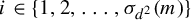
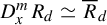
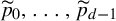
The Hubbard tree
 $H_-$
for
$H_-$
for
 $D_y^iR_d$
for
$D_y^iR_d$
for
 $-(d-1)\leq i\leq -1$
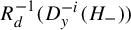
is the tree in Figure 4. The invariant angle between
$-(d-1)\leq i\leq -1$
is the tree in Figure 4. The invariant angle between
 $e_1$
and
$e_1$
and
 $e_2$
(measured counterclockwise) has measure
$e_2$
(measured counterclockwise) has measure
 $ - {2\pi i}/{d} = {2 \pi |i|}/{d}$
. The Hubbard tree
$ - {2\pi i}/{d} = {2 \pi |i|}/{d}$
. The Hubbard tree
 $H_+$
for
$H_+$
for
 $D_y^iR_d$
for
$D_y^iR_d$
for
 $1\leq i\leq d-1$
is the tree in Figure 5. The invariant angle between
$1\leq i\leq d-1$
is the tree in Figure 5. The invariant angle between
 $e^{\prime }_1$
and
$e^{\prime }_1$
and
 $e_2$
(measured counterclockwise) has measure
$e_2$
(measured counterclockwise) has measure
 $2\pi - {2\pi i}/{d}$
. Figure 4 demonstrates that
$2\pi - {2\pi i}/{d}$
. Figure 4 demonstrates that
 $H_-$
is invariant under
$H_-$
is invariant under
 $R_5^{-1}D_y$
, and Figure 5 demonstrates that
$R_5^{-1}D_y$
, and Figure 5 demonstrates that
 $H_+$
is invariant under
$H_+$
is invariant under
 $R_5^{-1}D_y^{-1}$
; the proof below explains that the figures generalize for all
$R_5^{-1}D_y^{-1}$
; the proof below explains that the figures generalize for all
 $d\geq 2$
, and for
$d\geq 2$
, and for
 $-(d-1)\leq i\leq -1$
and
$-(d-1)\leq i\leq -1$
and
 $1\leq i\leq d-1$
, respectively.
$1\leq i\leq d-1$
, respectively.
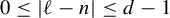
(a) The Hubbard tree
 $H_-$
for
$H_-$
for
 $D^i_yR_d$
with
$D^i_yR_d$
with
 $-(d-1)\leq i\leq -1$
. (b) A tree that is homotopic to
$-(d-1)\leq i\leq -1$
. (b) A tree that is homotopic to
 $D_y(H_-)$
. (c) A tree that is homotopic to the preimage of
$D_y(H_-)$
. (c) A tree that is homotopic to the preimage of
 $D_y(H_-)$
under
$D_y(H_-)$
under
 $R_5$
.
$R_5$
.

(a) The Hubbard tree
 $H_+$
for
$H_+$
for
 $D^i_yR_d$
with
$D^i_yR_d$
with
 $1\leq i\leq d-1$
. (b) A tree that is homotopic to
$1\leq i\leq d-1$
. (b) A tree that is homotopic to
 $D_y^{-1}(H_+)$
. (c) A tree that is homotopic to the preimage of
$D_y^{-1}(H_+)$
. (c) A tree that is homotopic to the preimage of
 $D_y^{-1}(H_+)$
under
$D_y^{-1}(H_+)$
under
 $R_5$
.
$R_5$
.

Proof. Let b be a special branch cut for
 $R_d$
(for instance, the arc b in Figure 4). By the definition of special branch cut, the preimage
$R_d$
(for instance, the arc b in Figure 4). By the definition of special branch cut, the preimage
 $R_d^{-1}(b)$
consists of d arcs from
$R_d^{-1}(b)$
consists of d arcs from
 $p_0$
to
$p_0$
to
 $\infty $
such that the complement of
$\infty $
such that the complement of
 $R_d^{-1}(b)$
in
$R_d^{-1}(b)$
in
 $\mathbb {C}$
contains d components and one of them contains both points
$\mathbb {C}$
contains d components and one of them contains both points
 $p_1$
and
$p_1$
and
 $p_2$
. Label these complementary components by
$p_2$
. Label these complementary components by
 $\Gamma _0,\ldots , \Gamma _{d-1}$
counterclockwise where
$\Gamma _0,\ldots , \Gamma _{d-1}$
counterclockwise where
 $\Gamma _0$
is the component that contains
$\Gamma _0$
is the component that contains
 $p_1$
and
$p_1$
and
 $p_2$
. The set
$p_2$
. The set
 $R_d^{-1}(p_0)$
contains d points; name them
$R_d^{-1}(p_0)$
contains d points; name them
 $\widetilde {p}_0,\ldots ,\widetilde {p}_{d-1}$
such that
$\widetilde {p}_0,\ldots ,\widetilde {p}_{d-1}$
such that
 $\widetilde {p}_j\in \Gamma _j$
.
$\widetilde {p}_j\in \Gamma _j$
.
We will show that
 $H_-$
is the Hubbard tree for
$H_-$
is the Hubbard tree for
 $D_y^iR_d$
when
$D_y^iR_d$
when
 $-(d-1)\leq i\leq 1$
and
$-(d-1)\leq i\leq 1$
and
 $H_+$
is the Hubbard tree for
$H_+$
is the Hubbard tree for
 $D_y^iR_d$
when
$D_y^iR_d$
when
 $1\leq i\leq d-1$
using the same basic strategy. First, we take the lift of the tree
$1\leq i\leq d-1$
using the same basic strategy. First, we take the lift of the tree
 $D_{y}^{-i}(H_\pm )$
under
$D_{y}^{-i}(H_\pm )$
under
 $R_d$
by computing the path lifts of the edges of
$R_d$
by computing the path lifts of the edges of
 $H_\pm $
(the edges of
$H_\pm $
(the edges of
 $H_-$
are
$H_-$
are
 $e_1$
and
$e_1$
and
 $e_2$
in
$e_2$
in
 $H_-$
, the edges of
$H_-$
, the edges of
 $H_+$
are
$H_+$
are
 $e^{\prime }_1$
and
$e^{\prime }_1$
and
 $e_2$
) and determining which are in the hull of
$e_2$
) and determining which are in the hull of
 $p_0,p_1,$
and
$p_0,p_1,$
and
 $p_2$
. We then verify the desired angle assignment is invariant under lifting.
$p_2$
. We then verify the desired angle assignment is invariant under lifting.
We first treat the case where
 $-(d-1)\leq i\leq -1$
. Note that i is negative so
$-(d-1)\leq i\leq -1$
. Note that i is negative so
 $D_y^{-i}$
is a positive (left-handed) twist. Observe that
$D_y^{-i}$
is a positive (left-handed) twist. Observe that
 $e_1$
is invariant under
$e_1$
is invariant under
 $D_y^{-i}$
for all i. The edge
$D_y^{-i}$
for all i. The edge
 $D_y^{-i}(e_2)$
intersects the branch cut b with both algebraic and geometric intersection i (with appropriately chosen orientations of b and
$D_y^{-i}(e_2)$
intersects the branch cut b with both algebraic and geometric intersection i (with appropriately chosen orientations of b and
 $e_2$
). That is, all intersections of
$e_2$
). That is, all intersections of
 $D_y^{-i}(e_2)$
and b have the same orientation (this an arc version of [Reference Farb and Margalit9, Proposition 3.2]).
$D_y^{-i}(e_2)$
and b have the same orientation (this an arc version of [Reference Farb and Margalit9, Proposition 3.2]).
For each
 $0\leq j\leq d-1$
, there is a path lift of
$0\leq j\leq d-1$
, there is a path lift of
 $D_y^{-i}(e_1)=e_1$
based at
$D_y^{-i}(e_1)=e_1$
based at
 $\widetilde {p}_j$
, call it
$\widetilde {p}_j$
, call it
 $\widetilde {e}_j$
. Because the interior of
$\widetilde {e}_j$
. Because the interior of
 $e_1$
is disjoint from the branch cut b, each
$e_1$
is disjoint from the branch cut b, each
 $\widetilde {e}_j$
is a straight line segment from
$\widetilde {e}_j$
is a straight line segment from
 $\widetilde {p}_j$
to
$\widetilde {p}_j$
to
 $p_0=R_d^{-1}(p_1)$
that is contained in the closure of
$p_0=R_d^{-1}(p_1)$
that is contained in the closure of
 $\Gamma _j$
, as in Lemma 3.1. In particular,
$\Gamma _j$
, as in Lemma 3.1. In particular,
 $\widetilde {e}_0$
is contained in the closure of
$\widetilde {e}_0$
is contained in the closure of
 $\Gamma _0$
and has endpoints
$\Gamma _0$
and has endpoints
 $p_0$
and
$p_0$
and
 $p_2$
. Since
$p_2$
. Since
 $\widetilde {e}_0$
is homotopic to a straight line segment relative to
$\widetilde {e}_0$
is homotopic to a straight line segment relative to
 $\{p_0, p_1, p_2\}$
, it is homotopic to
$\{p_0, p_1, p_2\}$
, it is homotopic to
 $e_2$
.
$e_2$
.
The arc
 $D_y^{-i}(e_2)$
twists counterclockwise
$D_y^{-i}(e_2)$
twists counterclockwise
 $|i|$
times around
$|i|$
times around
 $e_1$
(when oriented from
$e_1$
(when oriented from
 $p_0$
to
$p_0$
to
 $p_2$
). For each
$p_2$
). For each
 $0\leq j\leq d-1$
, there is a path lift of
$0\leq j\leq d-1$
, there is a path lift of
 $D_y^{-i}(e_2)$
based at
$D_y^{-i}(e_2)$
based at
 $\widetilde {p}_j$
with opposite endpoint in
$\widetilde {p}_j$
with opposite endpoint in
 $R_d^{-1}(p_2)$
; call this
$R_d^{-1}(p_2)$
; call this
 $\widetilde {E}_j$
. Each
$\widetilde {E}_j$
. Each
 $\widetilde {E}_j$
comprises a distinct component of
$\widetilde {E}_j$
comprises a distinct component of
 $R_d^{-1} (D_y^{-i}(e_2))$
. Moreover, each
$R_d^{-1} (D_y^{-i}(e_2))$
. Moreover, each
 $\widetilde {E}_j$
intersects
$\widetilde {E}_j$
intersects
 $R_d^{-1}(b)$
at
$R_d^{-1}(b)$
at
 $|i|$
points, rotating counterclockwise from
$|i|$
points, rotating counterclockwise from
 $\widetilde {p}_j$
to a point in
$\widetilde {p}_j$
to a point in
 $R^{-1}(p_2)$
. We may then apply Lemma 3.1 to determine that the opposite endpoint of
$R^{-1}(p_2)$
. We may then apply Lemma 3.1 to determine that the opposite endpoint of
 $\widetilde {E}_j$
is in
$\widetilde {E}_j$
is in
 $\Gamma _{(j+|i|)\mod d}$
.
$\Gamma _{(j+|i|)\mod d}$
.
The preimage
 $R_d^{-1}(D_y^{-i}(H_-))$
comprises the union of
$R_d^{-1}(D_y^{-i}(H_-))$
comprises the union of
 $\{\widetilde {e}_j\mid 0\leq j\leq d-1\}$
and
$\{\widetilde {e}_j\mid 0\leq j\leq d-1\}$
and
 $\{\widetilde {E}_j\mid 0\leq j\leq d-1\}$
. For each j, the union of
$\{\widetilde {E}_j\mid 0\leq j\leq d-1\}$
. For each j, the union of
 $\widetilde {e}_j$
and
$\widetilde {e}_j$
and
 $\widetilde {E}_j$
is a path between an element of
$\widetilde {E}_j$
is a path between an element of
 $R_d^{-1}(p_2)$
and
$R_d^{-1}(p_2)$
and
 $p_0$
(via
$p_0$
(via
 $\widetilde {p}_j$
). The only such path that is in the hull of
$\widetilde {p}_j$
). The only such path that is in the hull of
 $\{p_0,p_1,p_2\}$
in
$\{p_0,p_1,p_2\}$
in
 $R_d^{-1}(D_y^{-i}(H_-))$
is
$R_d^{-1}(D_y^{-i}(H_-))$
is
 $\widetilde {e}_{d+i}\cup \widetilde {E}_{d+i}$
, which contains
$\widetilde {e}_{d+i}\cup \widetilde {E}_{d+i}$
, which contains
 $p_1$
,
$p_1$
,
 $\widetilde {p}_{d+i}$
, and
$\widetilde {p}_{d+i}$
, and
 $p_0$
. This edge is homotopic to
$p_0$
. This edge is homotopic to
 $e_1$
. The other edge in the hull of
$e_1$
. The other edge in the hull of
 $\{p_0,p_1,p_2\}$
in
$\{p_0,p_1,p_2\}$
in
 $R_d^{-1}(D_y^{-i}(H_-))$
is
$R_d^{-1}(D_y^{-i}(H_-))$
is
 $\widetilde {e}_0$
, which has endpoints
$\widetilde {e}_0$
, which has endpoints
 $p_2$
and
$p_2$
and
 $p_0$
, and is homotopic to
$p_0$
, and is homotopic to
 $e_2$
. Thus, the tree
$e_2$
. Thus, the tree
 $H_-$
is invariant under lifting.
$H_-$
is invariant under lifting.
To see that the angle between
 $e_1$
and
$e_1$
and
 $e_2$
(measured counterclockwise) of
$e_2$
(measured counterclockwise) of
 $-{2\pi i}/{d}$
is invariant under
$-{2\pi i}/{d}$
is invariant under
 $D_y^iR_d$
for
$D_y^iR_d$
for
 $-(d-1)\leq i\leq -1$
, we track the preimage of all angles under the lifting process. In particular, we observe that the preimage of the angle between
$-(d-1)\leq i\leq -1$
, we track the preimage of all angles under the lifting process. In particular, we observe that the preimage of the angle between
 $e_1$
and
$e_1$
and
 $e_2$
is an angle at an unmarked vertex (of valence 2) in
$e_2$
is an angle at an unmarked vertex (of valence 2) in
 $R_d^{-1}(D_y^{-i}(H_-))$
, which is therefore irrelevant. However, because
$R_d^{-1}(D_y^{-i}(H_-))$
, which is therefore irrelevant. However, because
 $R_d^{-1}(p_1)=p_0$
, the preimage of the angle of
$R_d^{-1}(p_1)=p_0$
, the preimage of the angle of
 $2\pi $
at
$2\pi $
at
 $p_1$
(measured from
$p_1$
(measured from
 $e_1$
to itself) consists of d angles between the d path lifts of
$e_1$
to itself) consists of d angles between the d path lifts of
 $e_1$
, each of measure
$e_1$
, each of measure
 ${2\pi }/{d}$
. The path lifts of
${2\pi }/{d}$
. The path lifts of
 $e_1$
in the hull of
$e_1$
in the hull of
 $R_d^{-1}(D_y^{-i}(H_-))$
relative to
$R_d^{-1}(D_y^{-i}(H_-))$
relative to
 $\{0,p_1,p_2\}$
are
$\{0,p_1,p_2\}$
are
 $\widetilde {e}_0$
and
$\widetilde {e}_0$
and
 $\widetilde {e}_{d+i}$
. There are
$\widetilde {e}_{d+i}$
. There are
 $|i-1|$
path lifts of
$|i-1|$
path lifts of
 $e_1$
under
$e_1$
under
 $R_d$
between
$R_d$
between
 $\widetilde {e}_{d+i}$
and
$\widetilde {e}_{d+i}$
and
 $\widetilde {e}_0$
in the cyclic counterclockwise ordering of vertices adjacent to
$\widetilde {e}_0$
in the cyclic counterclockwise ordering of vertices adjacent to
 $p_0$
. Therefore, the angle between
$p_0$
. Therefore, the angle between
 $\widetilde {e}_0$
and
$\widetilde {e}_0$
and
 $\widetilde {e}_{d+i}$
is
$\widetilde {e}_{d+i}$
is
 ${2\pi |i|}/{d}$
, when measured counterclockwise. Since i is negative, the counterclockwise angle between the edges of the lift homotopic to
${2\pi |i|}/{d}$
, when measured counterclockwise. Since i is negative, the counterclockwise angle between the edges of the lift homotopic to
 $e_1$
and
$e_1$
and
 $e_2$
is
$e_2$
is
 $-{2\pi i}/{d}$
, and we have shown that
$-{2\pi i}/{d}$
, and we have shown that
 $D_y^iR_d$
is equivalent to
$D_y^iR_d$
is equivalent to
 $A_{d,-i}$
for
$A_{d,-i}$
for
 $-(d-1)\leq i\leq -1$
.
$-(d-1)\leq i\leq -1$
.
Now we show that the tree
 $H_+$
in Figure 5 is invariant under
$H_+$
in Figure 5 is invariant under
 $D_y^iR_d$
for
$D_y^iR_d$
for
 $1\leq i\leq d-1$
. Both edges
$1\leq i\leq d-1$
. Both edges
 $e^{\prime }_1$
and
$e^{\prime }_1$
and
 $e_2$
(in Figure 5) meet at the critical point
$e_2$
(in Figure 5) meet at the critical point
 $p_0$
. Orient both edges away from
$p_0$
. Orient both edges away from
 $p_0$
. The arcs
$p_0$
. The arcs
 $D_y^{-i}(e^{\prime }_1)$
and
$D_y^{-i}(e^{\prime }_1)$
and
 $D_y^{-i}(e_2)$
each intersect b in i points and all intersections have the same orientation (i.e., both arcs are directed clockwise at the points of intersection with b). For each
$D_y^{-i}(e_2)$
each intersect b in i points and all intersections have the same orientation (i.e., both arcs are directed clockwise at the points of intersection with b). For each
 $0\leq j\leq d-1$
, there is a path lift of
$0\leq j\leq d-1$
, there is a path lift of
 $D_y^{-i}(e_1)$
under
$D_y^{-i}(e_1)$
under
 $R_d$
based at
$R_d$
based at
 $\widetilde {p}_j$
and a path lift of
$\widetilde {p}_j$
and a path lift of
 $D_y^{-i}(e_2)$
based at
$D_y^{-i}(e_2)$
based at
 $\widetilde {p}_j$
; call these
$\widetilde {p}_j$
; call these
 $\widetilde {e}^{\prime }_j$
and
$\widetilde {e}^{\prime }_j$
and
 $\widetilde {E}^{\prime }_j$
, respectively. Each
$\widetilde {E}^{\prime }_j$
, respectively. Each
 $\widetilde {e}^{\prime }_j$
and
$\widetilde {e}^{\prime }_j$
and
 $\widetilde {E}^{\prime }_j$
intersects
$\widetilde {E}^{\prime }_j$
intersects
 $R_d^{-1}(b)$
at i points in a clockwise direction until it reaches its other endpoint. The other endpoint of
$R_d^{-1}(b)$
at i points in a clockwise direction until it reaches its other endpoint. The other endpoint of
 $\widetilde {E}^{\prime }_j$
is an element of
$\widetilde {E}^{\prime }_j$
is an element of
 $R_d^{-1}(p_2)$
and by Lemma 3.1, this endpoint is in
$R_d^{-1}(p_2)$
and by Lemma 3.1, this endpoint is in
 $\Gamma _{(j-i)\mod d}$
. The other endpoint of
$\Gamma _{(j-i)\mod d}$
. The other endpoint of
 $\widetilde {e}^{\prime }_j$
is
$\widetilde {e}^{\prime }_j$
is
 $p_0$
for all j. Then,
$p_0$
for all j. Then,
 $\widetilde {e}^{\prime }_0$
, which has endpoints
$\widetilde {e}^{\prime }_0$
, which has endpoints
 $p_2$
and
$p_2$
and
 $p_0$
, is in the hull of
$p_0$
, is in the hull of
 $\{p_0,p_1,p_2\}$
in
$\{p_0,p_1,p_2\}$
in
 $R_d^{-1}(D_y^{-i}(H_+))$
. In fact, as long as
$R_d^{-1}(D_y^{-i}(H_+))$
. In fact, as long as
 $1\leq i\leq d-1$
,
$1\leq i\leq d-1$
,
 $\widetilde {e}^{\prime }_0$
is homotopic to a straight line segment, that is,
$\widetilde {e}^{\prime }_0$
is homotopic to a straight line segment, that is,
 $e_2$
. Moreover, the union of
$e_2$
. Moreover, the union of
 $\widetilde {E}^{\prime }_i$
and
$\widetilde {E}^{\prime }_i$
and
 $\widetilde {e}^{\prime }_i$
forms an edge from
$\widetilde {e}^{\prime }_i$
forms an edge from
 $p_1$
to
$p_1$
to
 $p_0$
(via
$p_0$
(via
 $\widetilde {p}_i$
). As long as
$\widetilde {p}_i$
). As long as
 $1\leq i\leq d-1$
, this edge is homotopic to
$1\leq i\leq d-1$
, this edge is homotopic to
 $e^{\prime }_1$
.
$e^{\prime }_1$
.
As in the case where
 $-(d-1)\leq i\leq -1$
, to verify that the angle
$-(d-1)\leq i\leq -1$
, to verify that the angle
 $2\pi - {2\pi i}/{d}$
between
$2\pi - {2\pi i}/{d}$
between
 $e^{\prime }_1$
and
$e^{\prime }_1$
and
 $e_2$
(measured counterclockwise) is invariant under
$e_2$
(measured counterclockwise) is invariant under
 $R_d^{-1}D_y^{-i}$
, we need only consider the angle between the path lifts of
$R_d^{-1}D_y^{-i}$
, we need only consider the angle between the path lifts of
 $e^{\prime }_1$
that are in the hull of
$e^{\prime }_1$
that are in the hull of
 $\{p_0,p_1,p_2\}$
. Indeed, we saw above that
$\{p_0,p_1,p_2\}$
. Indeed, we saw above that
 $\widetilde {e}^{\prime }_0$
is always homotopic to
$\widetilde {e}^{\prime }_0$
is always homotopic to
 $e_2$
and
$e_2$
and
 $\widetilde {e}^{\prime }_i$
is part of the path in
$\widetilde {e}^{\prime }_i$
is part of the path in
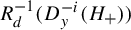 $R_d^{-1}(D_y^{-i}(H_+))$
that is homotopic to
$R_d^{-1}(D_y^{-i}(H_+))$
that is homotopic to
 $e^{\prime }_1$
. The angle between
$e^{\prime }_1$
. The angle between
 $\widetilde {e}^{\prime }_i$
and
$\widetilde {e}^{\prime }_i$
and
 $\widetilde {e}^{\prime }_0$
(measured counterclockwise) then has measure
$\widetilde {e}^{\prime }_0$
(measured counterclockwise) then has measure
 $2\pi -{2\pi i}/{d}$
, as desired. Therefore,
$2\pi -{2\pi i}/{d}$
, as desired. Therefore,
 $H_+$
with angle measure
$H_+$
with angle measure
 $2\pi - {2\pi i}/{d}$
between
$2\pi - {2\pi i}/{d}$
between
 $e^{\prime }_1$
and
$e^{\prime }_1$
and
 $e_2$
is invariant under
$e_2$
is invariant under
 $R_d^{-1}D_y^{-i}$
when
$R_d^{-1}D_y^{-i}$
when
 $1\leq i\leq d-1$
. Thus,
$1\leq i\leq d-1$
. Thus,
 $D_y^iR_d$
is equivalent to
$D_y^iR_d$
is equivalent to
 $A_{d,d-i}$
for
$A_{d,d-i}$
for
 $1\leq i\leq d-1$
.
$1\leq i\leq d-1$
.
Lemma 4.2. For all
 $d\geq 2$
, the branched cover
$d\geq 2$
, the branched cover
 $D_x^{-1}R_d$
is equivalent to
$D_x^{-1}R_d$
is equivalent to
 $\overline {R}_d$
.
$\overline {R}_d$
.
(a) The Hubbard tree H for
 $D_x^{-1}R_d$
. (b)
$D_x^{-1}R_d$
. (b)
 $D_x(H)$
. (c)
$D_x(H)$
. (c)
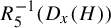 $R_5^{-1}(D_x(H))$
.
$R_5^{-1}(D_x(H))$
.

Proof. Figure 6 shows the Hubbard tree H for
 $D_x^{-1}R_d$
for all
$D_x^{-1}R_d$
for all
 $d\geq 2$
. Figure 6 also shows that the lift of
$d\geq 2$
. Figure 6 also shows that the lift of
 $D_x(H)$
under
$D_x(H)$
under
 $R_5$
is homotopic to H; a similar calculation verifies that the lift of
$R_5$
is homotopic to H; a similar calculation verifies that the lift of
 $D_x(H)$
under
$D_x(H)$
under
 $R_d$
is homotopic to H for all
$R_d$
is homotopic to H for all
 $d\geq 2$
. The angle assignment of
$d\geq 2$
. The angle assignment of
 $2\pi /3$
at each angle of the trivalent vertex is invariant under lifting. There are no Julia edges, so Poirier’s conditions verify that H is indeed the Hubbard tree of
$2\pi /3$
at each angle of the trivalent vertex is invariant under lifting. There are no Julia edges, so Poirier’s conditions verify that H is indeed the Hubbard tree of
 $D_x^{-1}R_d$
. Moreover,
$D_x^{-1}R_d$
. Moreover,
 $D_x^{-1}R_d$
rotates the edges clockwise relative to the trivalent vertex (one edge and its lift is dashed to assist tracking the rotation). Therefore,
$D_x^{-1}R_d$
rotates the edges clockwise relative to the trivalent vertex (one edge and its lift is dashed to assist tracking the rotation). Therefore,
 $D_x^{-1}R_d$
is equivalent to
$D_x^{-1}R_d$
is equivalent to
 $\overline {R}_d$
for
$\overline {R}_d$
for
 $d\geq 2$
.
$d\geq 2$
.
5 Proof of main theorem
We now combine the reduction formulas from §3 and the base cases from §4 to prove Theorem 1.1.
Proof of Theorem 1.1
As in the theorem, we consider the map
 $D_x^mR_d$
. Consider the
$D_x^mR_d$
. Consider the
 $d^2$
-adic expansion of m, which is
$d^2$
-adic expansion of m, which is
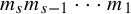 $m_sm_{s-1}\cdots m_1$
if
$m_sm_{s-1}\cdots m_1$
if
 $m\geq 0$
and
$m\geq 0$
and
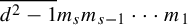 $\overline {d^2-1}m_sm_{s-1}\cdots m_1$
if
$\overline {d^2-1}m_sm_{s-1}\cdots m_1$
if
 $m<0$
.
$m<0$
.
We may write
 $m $
uniquely as
$m $
uniquely as
 $$ \begin{align*} m=d^2k_1+ d\ell_1 +n_1, \end{align*} $$
where
 $k_1\in \mathbb {Z}$
,
$k_1\in \mathbb {Z}$
,
 $\ell _1,n_1 \in \{0,1,\ldots ,d-1\}$
. We note that
$\ell _1,n_1 \in \{0,1,\ldots ,d-1\}$
. We note that
 $$ \begin{align*}k_1=\frac{m-m_1}{d^2}\quad\text{and}\quad m_1=d\ell_1+n_1.\end{align*} $$
For
 $2\leq i \leq s$
, there exist integers
$2\leq i \leq s$
, there exist integers
 $k_i \in \mathbb {Z}$
,
$k_i \in \mathbb {Z}$
,
 $0 \leq \ell _i, n_i \leq d-1$
such that
$0 \leq \ell _i, n_i \leq d-1$
such that
 $$ \begin{align*} k_{i} &= \frac{k_{i-1}-m_i}{d^2},\\ m_i & = d\ell_i + n_i,\quad\text{and }\\ k_{i-1} &= d^2k_i + d\ell_i + n_i. \end{align*} $$
That is, the
 $d^2$
-adic expansion of
$d^2$
-adic expansion of
 $k_i$
is obtained from m by dropping the right-most i digits. In particular, if
$k_i$
is obtained from m by dropping the right-most i digits. In particular, if
 $m\geq 0$
, then
$m\geq 0$
, then
 $k_s=0$
. If
$k_s=0$
. If
 $m<0$
, then
$m<0$
, then
 $k_s$
has
$k_s$
has
 $d^2$
-adic expansion
$d^2$
-adic expansion
 $\overline {d^2-1}$
and therefore
$\overline {d^2-1}$
and therefore
 $k_s=-1$
. Furthermore, we note that
$k_s=-1$
. Furthermore, we note that
 $\ell _i=n_i$
if and only if
$\ell _i=n_i$
if and only if
 $(d+1)|m_i$
.
$(d+1)|m_i$
.
By applying Lemma 3.2 to
 $D_x^mR_d$
, we have
$D_x^mR_d$
, we have
 $$ \begin{align*} D_x^mR_d \simeq \begin{cases} D_x^{k_1}R_d &\text{if } (d+1)|m_1,\\ D_y^{\ell_1-n_1}R_d & \text{otherwise.} \end{cases} \end{align*} $$
Thus, if
 $(d+1)\nmid m_1$
, we may apply Proposition 4.1, to obtain
$(d+1)\nmid m_1$
, we may apply Proposition 4.1, to obtain
 $$ \begin{align*} D_x^mR_d\simeq D_y^{\ell_1-n_1}R_d & = \begin{cases} A_{d,n_1-\ell_1} &\text{if } n_1>\ell_1,\\ A_{d,d-(\ell_1-n_1)} &\text{if } n_1<\ell_1. \end{cases} \end{align*} $$
So we can deduce the equivalence class of
 $D_x^mR_d$
directly if
$D_x^mR_d$
directly if
 $\ell _1 \neq n_1$
. Otherwise, we right-shift the
$\ell _1 \neq n_1$
. Otherwise, we right-shift the
 $d^2$
-adic expansion of m and consider
$d^2$
-adic expansion of m and consider
 $D_x^{k_1}R_d$
instead. We repeat this process for
$D_x^{k_1}R_d$
instead. We repeat this process for
 $k_1,\ldots ,k_s$
. Then, one of the following will occur.
$k_1,\ldots ,k_s$
. Then, one of the following will occur.
-
• If
$(d+1)|m_i$
for all i, then
$\ell _i=n_i$
for all i. In particular,
$\ell _s=n_s$
and we have
$$ \begin{align*} D_x^mR_d\simeq D_x^{k_1}R_d\simeq D_x^{k_2}R_d\simeq\cdots \simeq D_x^{k_{s-1}}R_d\simeq D_x^{k_s}R_d. \end{align*} $$
If
$m\geq 0$
, then
$k_s=0$
, so
$D_x^mR_d\simeq D_x^{k_s}R_d\simeq R_d$
.If
$m<0$
, then
$k_s=\overline {d^2-1}=-1$
and
$D_x^mR_d\simeq D_x^{k_s}R_d\simeq D_x^{-1}R_d$
. By Lemma 4.2,
$D_x^{-1}R_d$
is equivalent to
$\overline {R}_d$
. -
• If there exists i such that
$d+1$
does not divide
$m_i$
, choose the minimal such i and write
$m_i = d\ell _i+n_i$
, with
$\ell _i, n_i \in \{0,1,\ldots ,d-1\}$
. Then,
$\ell _i \neq n_i$
. Thus, by Proposition 4.1, we have
$$ \begin{align*} D_x^mR_d \simeq D_y^{\ell_i-n_i}R_d \simeq \begin{cases} A_{d,n_i-\ell_i}&\text{if } n_i>\ell_i,\\ A_{d,d-(\ell_i-n_i)} &\text{if } n_i<\ell_i. \end{cases} \end{align*} $$


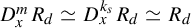

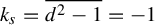
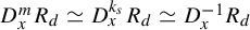


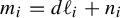


This completes the proof of the theorem.
Acknowledgements
The authors would like to thank Justin Lanier and Dan Margalit for comments on a draft of this paper. The authors would like to also thank the anonymous referee for their suggestions. This material is based upon work supported by the National Science Foundation under Grant No. DMS-1928930 while the authors participated in a program hosted by the Mathematical Sciences Research Institute in Berkeley, California, during Spring 2022. The second author was supported by the National Science Foundation under Grant No. DMS-2002951.
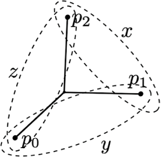
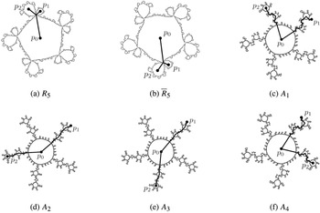

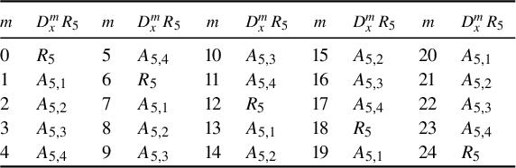


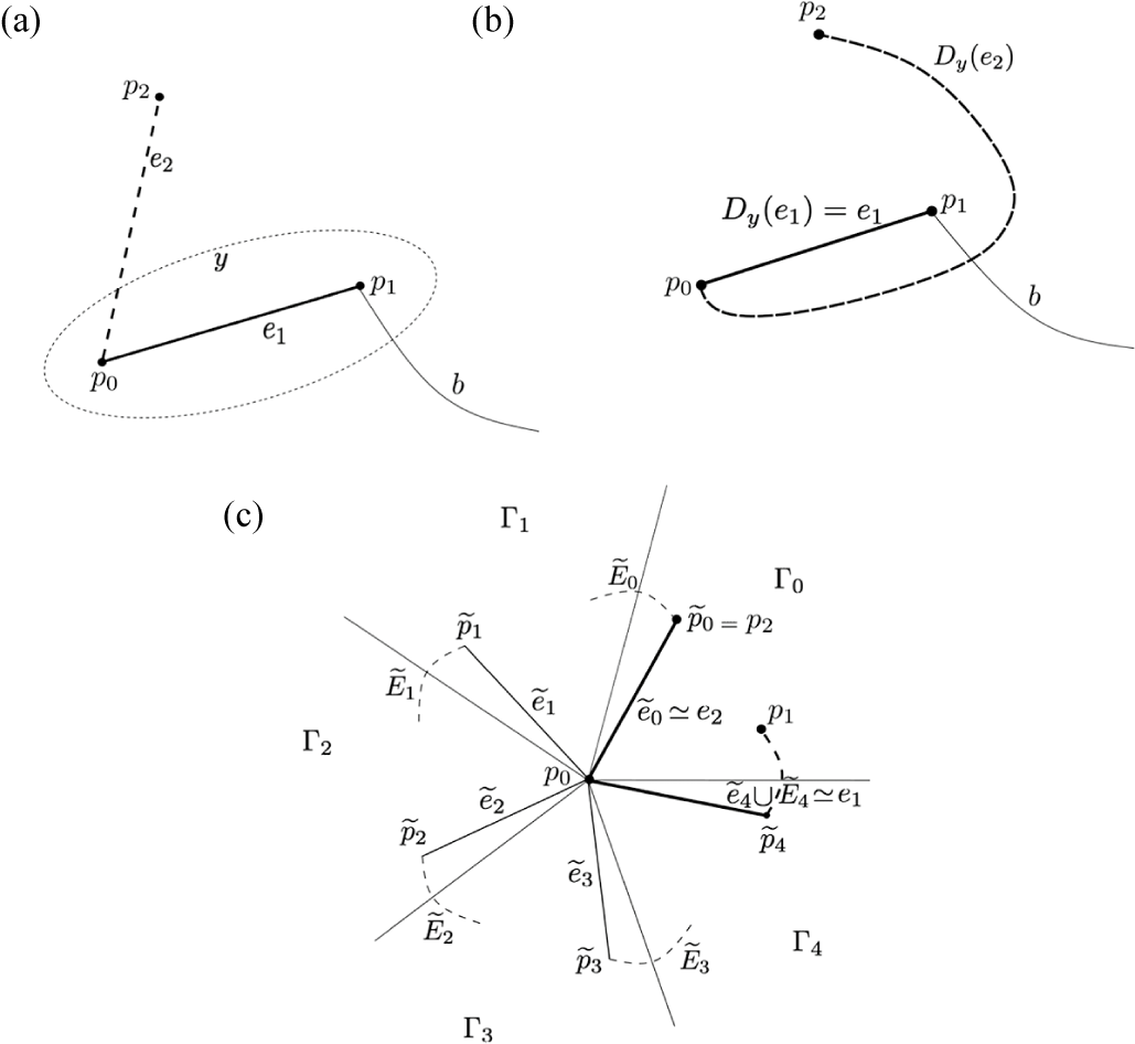


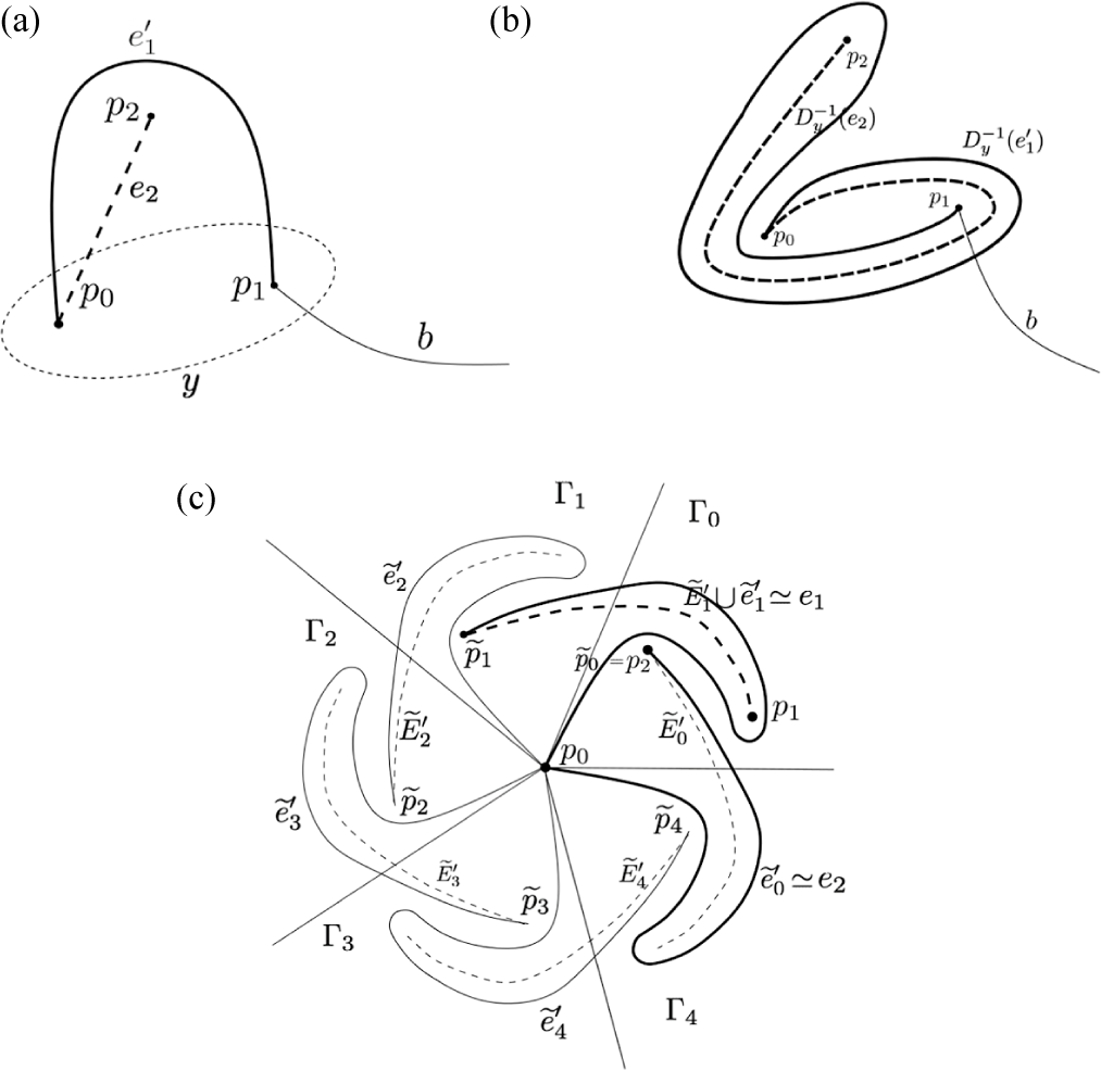


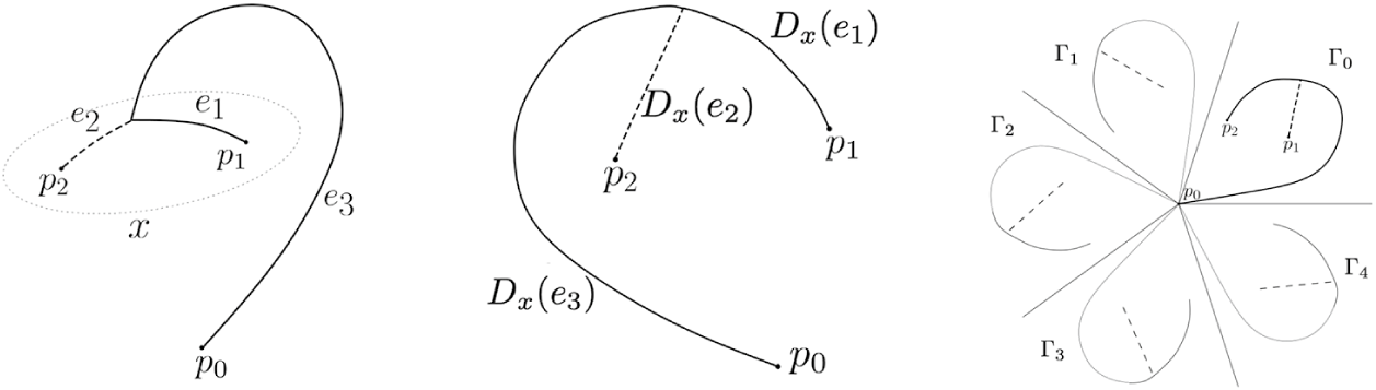


 Open access