


1. Introduction
In this second paper, we consider the evolution problem detailed in part 1 of this series of papers [Reference Needham, Billingham, Ladas and Meyer16] (and henceforth referred to as (NB1)) for the nonlocal Fisher-Kolmogorov-Petrovsky-Piskunov (Fisher-KPP) equation with top hat kernel, but now on a finite spatial interval $[0,a]$
, where
$[0,a]$
, where $a$
is the dimensionless interval length, scaled relative to the nonlocal length scale. In particular, this paper is designated as part 2 because it requires significant use and development of the theory and results detailed in part 1. As a consequence, the present paper should be read in conjunction with (NB1) to avoid significant repetition at numerous points throughout the paper. Reference to the relevant parts of (NB1) is clearly designated at all stages. As described in (NB1) and references therein, nonlocal reaction-diffusion equations arise in many different scientific areas, and finite domain effects can be relevant in a significant number of them, particularly in biomedical applications, [Reference Banerjee, Kuznetsov, Udovenko and Volpert2]. The reader is referred to the introduction of (NB1) for a more extensive and general discussion of background and related works, which need not be repeated here. In this regard, we note that the majority of significant theoretical works on the nonlocal Fisher-KPP equation have treated the Cauchy problem on the real line, in respect to travelling wave-fronts, spreading speeds and stationary patterning, and as such have been referenced and discussed in the introduction and relevant sections of (NB1) (we mention here [Reference Berestycki, Nadin, Perthame and Ryzhik3], [Reference Volpert20], [Reference Hamel and Ryzhik11], [Reference Faye and Holzer8], [Reference Li, Chen and Surulescu13], [Reference Bouin, Henderson and Ryzhik5], [Reference Fang and Zhao7], [Reference Volpert, Vougalter, Lewis, Maini and Petrovsky19] and [Reference Li, Chen and Surulescu13]). However, it is appropriate to contextualise here the relevance of considering the evolution problem on a finite spatial interval, with associated Dirichlet or Neumann boundary conditions. Specifically, from a modelling perspective, the relevance of finite interval problems arises naturally in ecological population dynamics and many biomedical applications. Modelling and analysis in these areas have recently been developed in [Reference Dornelas, Colombo, Lopez, Hernandez-Garcia and Anteneodo6] and [Reference Jewell, Krause, Maini and Gaffney12]. Also, it is worth emphasising that the key feature of the inclusion of the nonlocal term is the introduction of a nonlocal length scale into the model. There are thus two dimensionless parameters in the model, namely
$a$
is the dimensionless interval length, scaled relative to the nonlocal length scale. In particular, this paper is designated as part 2 because it requires significant use and development of the theory and results detailed in part 1. As a consequence, the present paper should be read in conjunction with (NB1) to avoid significant repetition at numerous points throughout the paper. Reference to the relevant parts of (NB1) is clearly designated at all stages. As described in (NB1) and references therein, nonlocal reaction-diffusion equations arise in many different scientific areas, and finite domain effects can be relevant in a significant number of them, particularly in biomedical applications, [Reference Banerjee, Kuznetsov, Udovenko and Volpert2]. The reader is referred to the introduction of (NB1) for a more extensive and general discussion of background and related works, which need not be repeated here. In this regard, we note that the majority of significant theoretical works on the nonlocal Fisher-KPP equation have treated the Cauchy problem on the real line, in respect to travelling wave-fronts, spreading speeds and stationary patterning, and as such have been referenced and discussed in the introduction and relevant sections of (NB1) (we mention here [Reference Berestycki, Nadin, Perthame and Ryzhik3], [Reference Volpert20], [Reference Hamel and Ryzhik11], [Reference Faye and Holzer8], [Reference Li, Chen and Surulescu13], [Reference Bouin, Henderson and Ryzhik5], [Reference Fang and Zhao7], [Reference Volpert, Vougalter, Lewis, Maini and Petrovsky19] and [Reference Li, Chen and Surulescu13]). However, it is appropriate to contextualise here the relevance of considering the evolution problem on a finite spatial interval, with associated Dirichlet or Neumann boundary conditions. Specifically, from a modelling perspective, the relevance of finite interval problems arises naturally in ecological population dynamics and many biomedical applications. Modelling and analysis in these areas have recently been developed in [Reference Dornelas, Colombo, Lopez, Hernandez-Garcia and Anteneodo6] and [Reference Jewell, Krause, Maini and Gaffney12]. Also, it is worth emphasising that the key feature of the inclusion of the nonlocal term is the introduction of a nonlocal length scale into the model. There are thus two dimensionless parameters in the model, namely $D$
, which measures the square of the ratio of the diffusion length scale (based on the kinetic time scale) to the nonlocal length scale, and
$D$
, which measures the square of the ratio of the diffusion length scale (based on the kinetic time scale) to the nonlocal length scale, and $a$
, which measures the ratio of the domain length scale to the nonlocal length scale. We examine both the Dirichlet and the Neumann models for
$a$
, which measures the ratio of the domain length scale to the nonlocal length scale. We examine both the Dirichlet and the Neumann models for $(a,D)$
throughout the positive quadrant of the parameter plane. As should be expected, significant structural differences in behaviour between the classical Fisher-KPP model and this natural nonlocal extended model become more extensive as the parameter
$(a,D)$
throughout the positive quadrant of the parameter plane. As should be expected, significant structural differences in behaviour between the classical Fisher-KPP model and this natural nonlocal extended model become more extensive as the parameter $D$
decreases and the nonlocal length scale becomes dominant (the classical local Fisher-KPP models are readily recovered, after a rescaling of dimensionless length with
$D$
decreases and the nonlocal length scale becomes dominant (the classical local Fisher-KPP models are readily recovered, after a rescaling of dimensionless length with $\sqrt {D}$
, in the limit
$\sqrt {D}$
, in the limit $D\to \infty$
, uniformly for
$D\to \infty$
, uniformly for $a\gt 0$
), and these principal, and marked, differences are fully explored, exposed and summarised at the end of each section and subsection. We remark here that throughout the paper, we regard
$a\gt 0$
), and these principal, and marked, differences are fully explored, exposed and summarised at the end of each section and subsection. We remark here that throughout the paper, we regard $a$
as a bifurcation parameter, at fixed
$a$
as a bifurcation parameter, at fixed $D$
, which is regarded as the unfolding parameter. For each fixed positive
$D$
, which is regarded as the unfolding parameter. For each fixed positive $D$
, we endeavour to give a complete description of the key qualitative and quantitative features of the model. To achieve this, we find it useful to adopt and develop a combination of well-established approaches as and when appropriate, including direct exact analysis, classical linearised and weakly nonlinear theory, local bifurcation theory, matched asymptotic methods and numerical approximation.
$D$
, we endeavour to give a complete description of the key qualitative and quantitative features of the model. To achieve this, we find it useful to adopt and develop a combination of well-established approaches as and when appropriate, including direct exact analysis, classical linearised and weakly nonlinear theory, local bifurcation theory, matched asymptotic methods and numerical approximation.
The simplicity of the top hat kernel allows us to develop both a qualitative and quantitative description of the strongly nonlinear and nonlocal structure and dynamics of the solution set to both the Dirichlet and Neumann models, whose qualitative features (strongly nonlinear and nonlocal hump formation and structure, and accumulating numbers of temporally stable multi-hump steady-state attractors), which have previously been unidentified, are expected to remain relevant for other localised kernels that are less amenable to this type of detailed analysis. In particular, we study, in detail, regimes far away from linear and weakly nonlinear limits, and address the fully nonlinear interaction between nonlocality, diffusion and competition in the underlying nonlocal PDE.
We address the evolution problem, firstly with Dirichlet and secondly with Neumann boundary conditions at the two ends of the finite spatial interval. The evolution problem is
 \begin{equation} u_t = Du_{xx} + u\left (1 - \int _{\alpha (x)}^{\beta (x)}{u(y,t)dy}\right )\,\,\text{with}\,\,(x,t)\in D_{\infty }, \end{equation}
with the domain
 \begin{equation} D_{\infty }=(0,a)\times (0,\infty ), \end{equation}
and where, with $0\lt a\le 1/2,$
we have,
$0\lt a\le 1/2,$
we have,
 \begin{equation} \alpha (x) = 0\,\,\text{and}\,\,\beta (x)=a\,\,\forall \,\,x\in [0,a], \end{equation}
whilst, with $a\gt 1/2,$
we have,
$a\gt 1/2,$
we have,
 \begin{equation} \alpha (x) = \begin{cases} 0,\,0\le x\le \dfrac {1}{2},\\[5pt] x-\dfrac {1}{2},\,\dfrac {1}{2}\lt x\le a, \end{cases} \end{equation}
and,
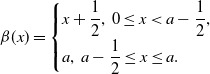 \begin{equation} \beta (x) = \begin{cases} x+\dfrac {1}{2},\,0\le x \lt a-\dfrac {1}{2},\\[5pt] a,\,a-\dfrac {1}{2}\le x \le a. \end{cases} \end{equation}
These two conditions simply ensure that the nonlocal range does not extend beyond the two boundaries of the finite interval. The associated initial condition is,
 \begin{equation} u(x,0)=u_0(x),\,x\in [0,a], \end{equation}
whilst the boundary conditions are, for the Dirichlet problem,
 \begin{equation} u(0,t) = u(a,t) = 0,\,t\in (0,\infty ), \end{equation}
or for the Neumann problem,
 \begin{equation} u_x(0,t)=u_x(a,t)=0,\,t\in (0,\infty ). \end{equation}
In the above, $D$
is the constant diffusion coefficient. The initial data have
$D$
is the constant diffusion coefficient. The initial data have $u_0\in C([0,a])\cap PC^1([0,a])$
(that is, continuous with piecewise continuous derivative), and are non-negative and nontrivial. We henceforth refer to the Dirichlet problem as (DIVP) and the Neumann problem as (NIVP), and throughout we will consider classical solutions to these two evolution problems.
$u_0\in C([0,a])\cap PC^1([0,a])$
(that is, continuous with piecewise continuous derivative), and are non-negative and nontrivial. We henceforth refer to the Dirichlet problem as (DIVP) and the Neumann problem as (NIVP), and throughout we will consider classical solutions to these two evolution problems.
To begin with, we review the basic setting in uniqueness and global existence for both of the evolution problems (DIVP) and (NIVP). To this end, it is a straightforward consequence of the parabolic strong maximum principle (and non-negative, nontrivial initial data) that, with $u\;:\;D_{\infty }\to \mathbb{R}$
being a solution to either of (DIVP) or (NIVP), then,
$u\;:\;D_{\infty }\to \mathbb{R}$
being a solution to either of (DIVP) or (NIVP), then,
 \begin{equation} u(x,t) \gt 0\,\,\forall \,\,(x,t)\in D_{\infty }. \end{equation}
It is then a consequence of the parabolic comparison theorem (with parabolic operator $N[u] \equiv u_t - Du_{xx} - u)$
that,
$N[u] \equiv u_t - Du_{xx} - u)$
that,
 \begin{equation} u(x,t) \le Me^t\,\,\forall \,\,(x,t)\in \overline {D} _{\infty }, \end{equation}
with $M=$
sup
$M=$
sup $_{y\in [0,a]}u_0(y)$
. The a priori bounds in (9) and (10) readily guarantee the existence and uniqueness of a classical solution to either of (DIVP) and (NIVP) (without repetition, this follows very closely from the discussion, and key references therein, as laid out in section 2 of (NB1) for the Cauchy problem on the real line). A further simple application of the parabolic comparison theorem establishes that, for the solution to (DIVP), there exists a positive constant
$_{y\in [0,a]}u_0(y)$
. The a priori bounds in (9) and (10) readily guarantee the existence and uniqueness of a classical solution to either of (DIVP) and (NIVP) (without repetition, this follows very closely from the discussion, and key references therein, as laid out in section 2 of (NB1) for the Cauchy problem on the real line). A further simple application of the parabolic comparison theorem establishes that, for the solution to (DIVP), there exists a positive constant $A$
, for which
$A$
, for which $u_0(x)\le A\sin \left (\frac {\pi x}{a}\right )\,\, \forall \,\, x\in [0,a]$
, and such that,
$u_0(x)\le A\sin \left (\frac {\pi x}{a}\right )\,\, \forall \,\, x\in [0,a]$
, and such that,
 \begin{equation} u(x,t) \le Ae^{\big(1-\frac {{\pi }^2D}{a^2}\big)t}\sin \left (\frac {\pi x}{a}\right )\,\,\forall \,\,(x,t)\in \overline {D}_{\infty }. \end{equation}
The remainder of the paper is structured as follows. Section 2 addresses (DIVP) in detail. Exact solutions are constructed for $0\lt a\le 1/2$
, which allow for a complete analysis of (DIVP). For
$0\lt a\le 1/2$
, which allow for a complete analysis of (DIVP). For $a\gt 1/2$
, we first consider the existence of nontrivial and non-negative steady states associated with (DIVP). We achieve this by fixing
$a\gt 1/2$
, we first consider the existence of nontrivial and non-negative steady states associated with (DIVP). We achieve this by fixing $D$
as an unfolding parameter and regarding
$D$
as an unfolding parameter and regarding $a$
as a bifurcation parameter. The detailed bifurcation structure is examined numerically via pseudo-arclength continuation (see Appendix A or [Reference Allgower and Georg1]), with the asymptotic structure of steady states examined in detail in a number of relevant limits in the positive quadrant of the
$a$
as a bifurcation parameter. The detailed bifurcation structure is examined numerically via pseudo-arclength continuation (see Appendix A or [Reference Allgower and Georg1]), with the asymptotic structure of steady states examined in detail in a number of relevant limits in the positive quadrant of the $(a,D)$
parameter plane through the use of well established regular and singular perturbation methods, the conclusions of which are gathered together in each relevant subsection. In this way, the intricate nature of this bifurcation structure is fully detailed across the primary linear and weakly nonlinear local bifurcations from the trivial steady state into the fully nonlinear and nonlocal multiple and accumulating secondary bifurcations. The linear stability of the multiple steady states generated from these accumulating secondary bifurcations is examined by analysis of the associated linear, nonlocal, variable coefficient and eigenvalue problem. This then enables us to make conjectures relating to the large-
$(a,D)$
parameter plane through the use of well established regular and singular perturbation methods, the conclusions of which are gathered together in each relevant subsection. In this way, the intricate nature of this bifurcation structure is fully detailed across the primary linear and weakly nonlinear local bifurcations from the trivial steady state into the fully nonlinear and nonlocal multiple and accumulating secondary bifurcations. The linear stability of the multiple steady states generated from these accumulating secondary bifurcations is examined by analysis of the associated linear, nonlocal, variable coefficient and eigenvalue problem. This then enables us to make conjectures relating to the large- $t$
attractors for (DIVP), and these conjectures are then supported by careful numerical solutions to (DIVP). In section 3, we follow a similar approach in developing a detailed analysis to (NIVP), and compare and contrast the results with the corresponding results in section 2. We draw some relevant conclusions in section 4. Throughout the paper, the key results and their relevance are summarised, discussed and contextualised at the end of each section and subsection. Descriptions of the numerical methods required and used in the paper are given in Appendix A.
$t$
attractors for (DIVP), and these conjectures are then supported by careful numerical solutions to (DIVP). In section 3, we follow a similar approach in developing a detailed analysis to (NIVP), and compare and contrast the results with the corresponding results in section 2. We draw some relevant conclusions in section 4. Throughout the paper, the key results and their relevance are summarised, discussed and contextualised at the end of each section and subsection. Descriptions of the numerical methods required and used in the paper are given in Appendix A.
2. The Dirichlet problem (DIVP)
In this section, we focus on the Dirichlet problem (DIVP). To begin with, we observe that when the initial data is trivial, the solution to the associated (DIVP) is the equilibrium solution
 \begin{equation} u(x,t)=u_e=0\,\,\forall \,\,(x,t)\in \bar {D}_{\infty }. \end{equation}
For initial data with $\parallel$ $u_0$
$u_0$ $\parallel _{\infty }$
small, it is straightforward to develop a linearised theory for (DIVP). For brevity, we do not present the details, which are standard, but observe that this linearised theory for (DIVP) leads directly to the conclusion that the trivial equilibrium solution is locally asymptotically stable when
$\parallel _{\infty }$
small, it is straightforward to develop a linearised theory for (DIVP). For brevity, we do not present the details, which are standard, but observe that this linearised theory for (DIVP) leads directly to the conclusion that the trivial equilibrium solution is locally asymptotically stable when $D\gt a^2/\pi ^2$
but unstable when
$D\gt a^2/\pi ^2$
but unstable when $0\lt D\lt a^2/\pi ^2$
. These conclusions can be extended, via (9) and (11), beyond the linearised regime to prove that the trivial equilibrium solution is globally asymptotically stable when
$0\lt D\lt a^2/\pi ^2$
. These conclusions can be extended, via (9) and (11), beyond the linearised regime to prove that the trivial equilibrium solution is globally asymptotically stable when $D\gt a^2/\pi ^2$
, and at least Liapunov stable when
$D\gt a^2/\pi ^2$
, and at least Liapunov stable when $D=a^2/\pi ^2.$
Thus, when
$D=a^2/\pi ^2.$
Thus, when $D\gt a^2/\pi ^2$
, the solution to (DIVP) decays to zero exponentially in
$D\gt a^2/\pi ^2$
, the solution to (DIVP) decays to zero exponentially in $t$
as
$t$
as $t\to \infty$
, uniformly for
$t\to \infty$
, uniformly for $x\in [0,a]$
. The remainder of this section focuses on considering the nature of the solution to (DIVP) when
$x\in [0,a]$
. The remainder of this section focuses on considering the nature of the solution to (DIVP) when $0\lt D\lt a^2/\pi ^2$
, and in particular the structure of the solution for
$0\lt D\lt a^2/\pi ^2$
, and in particular the structure of the solution for $t$
large. To continue, it is convenient to consider the cases when
$t$
large. To continue, it is convenient to consider the cases when $0\lt a\le 1/2$
and
$0\lt a\le 1/2$
and $a\gt 1/2$
separately.
$a\gt 1/2$
separately.
In addition, referring back to our observation in the introduction, we again note that in the limit $D \to \infty$
(after rescaling
$D \to \infty$
(after rescaling $x$
with
$x$
with $\sqrt {D}$
), (DIVP) formally becomes the classical local Fisher-KPP Dirichlet problem, and so we should expect that the associated well known classical results for this local problem are recovered in this limit, and this is confirmed in what follows.
$\sqrt {D}$
), (DIVP) formally becomes the classical local Fisher-KPP Dirichlet problem, and so we should expect that the associated well known classical results for this local problem are recovered in this limit, and this is confirmed in what follows.
2.1. $0\lt a\le 1/2$

In this case, it follows from (3) that equation (1) becomes,
 \begin{equation} u_t = Du_{xx} + u(1-a\bar{u}(t)),\,\,(x,t)\in D_{\infty }, \end{equation}
where $\bar {u}\;:\;[0,\infty )\to \mathbb{R}$
is the spatial mean value of
$\bar {u}\;:\;[0,\infty )\to \mathbb{R}$
is the spatial mean value of $u$
over the interval
$u$
over the interval $[0,a],$
given by,
$[0,a],$
given by,
 \begin{equation} \bar {u}(t) = \frac {1}{a} \int _0^a{u(y,t)}dy\,\,\forall \,\,t\in [0,\infty ). \end{equation}
Before considering (DIVP) in detail, it is instructive to first consider the possible non-negative and nontrivial steady states, which satisfy equation (13) and boundary conditions (7), as such steady states are potential attractors for the solution to (DIVP) as $t\to \infty$
when
$t\to \infty$
when $0\lt D\lt a^2/\pi ^2$
. A non-negative steady state
$0\lt D\lt a^2/\pi ^2$
. A non-negative steady state $u_s\;:\;[0,a]\to \mathbb{R}$
to (DIVP) satisfies,
$u_s\;:\;[0,a]\to \mathbb{R}$
to (DIVP) satisfies,
 \begin{equation} Du_s'' + u_s(1-a\bar {u}_s) = 0, \,\,x\in (0,a), \end{equation}
with,
 \begin{equation} u_s(x)\ge 0\,\,\forall \,\,x\in [0,a], \end{equation}
subject to the boundary conditions,
 \begin{equation} u_s(0)=u_s(a)=0, \end{equation}
and with the constant $\bar {u}_s$
given by,
$\bar {u}_s$
given by,
 \begin{equation} \bar {u}_s = \frac {1}{a}\int _0^a{u_s(y)}dy. \end{equation}
It is straightforward to analyse this boundary value problem directly, and the details are left to the reader. Apart from the trivial solution, it has an additional nontrivial solution if and only if $0\lt D\lt a^2/\pi ^2$
, and this solution is given by,
$0\lt D\lt a^2/\pi ^2$
, and this solution is given by,
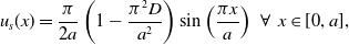 \begin{equation} u_s(x) = \frac {\pi }{2a}\left (1 - \frac {\pi ^2D}{a^2}\right )\sin \left (\frac {\pi x}{a}\right )\,\,\forall \,\,x\in [0,a], \end{equation}
with,
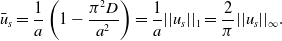 \begin{equation} \bar {u}_s = \frac {1}{a}\left (1 - \frac {\pi ^2D}{a^2}\right ) = \frac {1}{a}||u_s||_1 = \frac {2}{\pi }||u_s||_{\infty }. \end{equation}
We observe that the nontrivial steady state is a positive single hump, symmetric about $x=\frac {1}{2}a$
, and with support spanning the whole interval. It is convenient to consider this steady state with
$x=\frac {1}{2}a$
, and with support spanning the whole interval. It is convenient to consider this steady state with $0\lt D\lt 1/4\pi ^2$
fixed, and allowing
$0\lt D\lt 1/4\pi ^2$
fixed, and allowing $a$
to vary in the interval of existence
$a$
to vary in the interval of existence $(\pi \sqrt {D},1/2].$
In this context, from (19) and (20), we see directly that
$(\pi \sqrt {D},1/2].$
In this context, from (19) and (20), we see directly that $u_s$
emerges at a steady state transcritical bifurcation from the equilibrium state
$u_s$
emerges at a steady state transcritical bifurcation from the equilibrium state $u_e=0$
, when
$u_e=0$
, when $a=\pi \sqrt {D}$
(noting that the nontrivial steady solution generated by this bifurcation for
$a=\pi \sqrt {D}$
(noting that the nontrivial steady solution generated by this bifurcation for $a\in (0,\pi \sqrt {D})$
is negative, and thus ruled out) and develops for
$a\in (0,\pi \sqrt {D})$
is negative, and thus ruled out) and develops for $a\in (\pi \sqrt {D},1/2].$
For
$a\in (\pi \sqrt {D},1/2].$
For $1/12\pi ^2\le D\lt 1/4\pi ^2,$
we note that
$1/12\pi ^2\le D\lt 1/4\pi ^2,$
we note that $||u_s||_{\infty }$
is monotone increasing with
$||u_s||_{\infty }$
is monotone increasing with $a$
, whilst for
$a$
, whilst for $0\lt D\lt 1/12\pi ^2,$
we determine that now
$0\lt D\lt 1/12\pi ^2,$
we determine that now $||u_s||_\infty$
has a single maximum, at
$||u_s||_\infty$
has a single maximum, at $a=\sqrt {3}\pi \sqrt {D}$
, with value
$a=\sqrt {3}\pi \sqrt {D}$
, with value $||u_s||_\infty =1/(3^{\frac {3}{2}}\sqrt {D}).$
In Figure 1, we graph
$||u_s||_\infty =1/(3^{\frac {3}{2}}\sqrt {D}).$
In Figure 1, we graph $||u_s||_\infty$
against
$||u_s||_\infty$
against $a$
at a number of values of
$a$
at a number of values of $D.$
It is anticipated that, at fixed
$D.$
It is anticipated that, at fixed $0\lt D\le 1/4\pi ^2$
, this branch of steady solutions will be smoothly continued into
$0\lt D\le 1/4\pi ^2$
, this branch of steady solutions will be smoothly continued into $a\gt 1/2.$
This will be addressed at a later stage. For the present, we now return to considering (DIVP) in detail.
$a\gt 1/2.$
This will be addressed at a later stage. For the present, we now return to considering (DIVP) in detail.
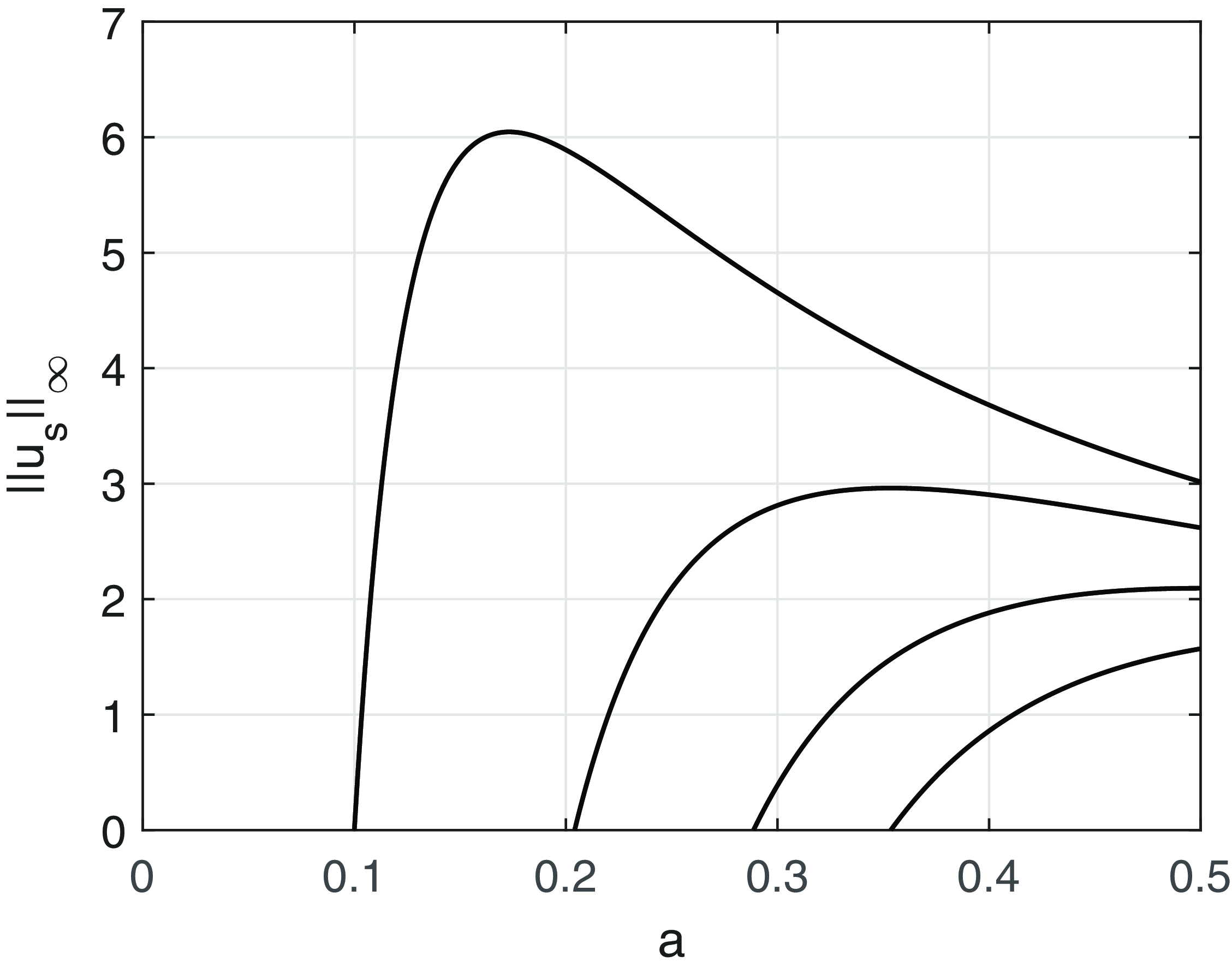
Figure 1. $||u_s||_{\infty }$
as a function of
$||u_s||_{\infty }$
as a function of $a$
for
$a$
for $\pi ^2 D = \frac {1}{100}$
,
$\pi ^2 D = \frac {1}{100}$
, $\frac {1}{24}$
,
$\frac {1}{24}$
, $\frac {1}{12}$
and
$\frac {1}{12}$
and $\frac {1}{8}$
.
$\frac {1}{8}$
.
With equation (1) now having the form given in (13), we can, in fact, directly construct the solution to (DIVP) as follows. First, we write the solution $u\;:\;\bar {D}_{\infty }\to \mathbb{R}$
to (DIVP), via Fourier’s Theorem, as,
$u\;:\;\bar {D}_{\infty }\to \mathbb{R}$
to (DIVP), via Fourier’s Theorem, as,
 \begin{equation} u(x,t) = \sum _{n=1}^{\infty }{A_{n}(t)\sin \left (\frac {n\pi x}{a}\right )}\,\,\forall \,\,(x,t)\in \bar {D}_{\infty }, \end{equation}
which satisfies the boundary conditions (7), and, for each $n\in \mathbb{N}$
,
$n\in \mathbb{N}$
, $A_n\;:\;[0,\infty )\to \mathbb{R}$
is to be determined so that (21) satisfies equation (13) and initial condition (6). For each
$A_n\;:\;[0,\infty )\to \mathbb{R}$
is to be determined so that (21) satisfies equation (13) and initial condition (6). For each $n\in \mathbb{N}$
, it follows from a direct substitution that this is achieved if and only if
$n\in \mathbb{N}$
, it follows from a direct substitution that this is achieved if and only if $A_n(t)$
satisfies the initial value problem,
$A_n(t)$
satisfies the initial value problem,
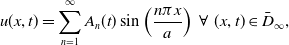
 \begin{equation} A_n'(t) = A_n(t) \left (1-D\frac {n^2\pi ^2}{a^2}-a\bar {u}(t)\right ),\,\,t\gt 0, \end{equation}
subject to,
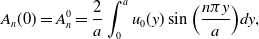 \begin{equation} A_n(0) = A_n^0 = \frac {2}{a}\int _0^a{u_0(y)\sin \left (\frac {n\pi y}{a}\right )}dy, \end{equation}
and we note, following the earlier conditions on $u_0,$
that
$u_0,$
that
 \begin{equation} A_1^0\gt 0, \end{equation}
whilst,
 \begin{equation} \bar {u}(0) = \frac {1}{a}\int _0^a{u_0(y)}dy = \frac {2}{\pi }\sum _{r=1}^{\infty }{\frac {A_{2r-1}^{0}}{(2r-1)}} \gt 0. \end{equation}
The solution to (22) and (23) is readily obtained as,
 \begin{equation} A_n(t) = A_n^0J(t)e^{-\frac {n^2\pi ^2D}{a^2}t},\,\,t\ge 0, \end{equation}
with,
 \begin{equation} J(t) = e^{(t - aI(t))}\gt 0,\,\,t\ge 0, \end{equation}
and,
 \begin{equation} I(t) = \int _0^t{\bar {u}(s)}ds,\,\,t\ge 0. \end{equation}
The solution to (DIVP) can now be written, via (21) and (26), as
 \begin{equation} u(x,t) = J(t)\sum _{n=1}^{\infty }A_n^0e^{-\frac {n^2\pi ^2D}{a^2}t}\sin \left (\frac {n\pi x}{a}\right ),\,\,(x,t)\in \bar {D}_{\infty }. \end{equation}
We note, via differentiating (27), that we may rearrange to obtain,
 \begin{equation} \bar {u}(t) = \frac {1}{a}\left (1 - \frac {J'(t)}{J(t)}\right ),\,\,t\ge 0, \end{equation}
and, via (27), that,
 \begin{equation} J(0) = 1. \end{equation}
Now, on integrating (29) across the spatial interval $[0,a]$
, we obtain,
$[0,a]$
, we obtain,
 \begin{equation} \bar {u}(t) = J(t)G(t),\,\,t\gt 0, \end{equation}
with $G\in C([0,\infty )) \cap C^{\infty }((0,\infty ))$
being the known function,
$G\in C([0,\infty )) \cap C^{\infty }((0,\infty ))$
being the known function,
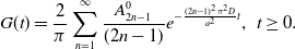 \begin{equation} G(t) = \frac {2}{\pi } \sum _{n=1}^{\infty }\frac {A_{2n-1}^0}{(2n-1)}e^{-\frac {(2n-1)^2\pi ^2D}{a^2}t},\,\,t\ge 0. \end{equation}
It follows from (27) and (32) (recalling from (9) that the solution to (DIVP) is strictly positive on $D_{\infty }$
) that,
$D_{\infty }$
) that,
 \begin{equation} G(t)\gt 0\,\,\forall \,\,t\ge 0, \end{equation}
and
 \begin{equation} G(0)=\bar {u}(0). \end{equation}
whilst,
 \begin{equation} G(t) \sim \frac {2}{\pi }A_1^0e^{-\frac {\pi ^2D}{a^2}t}\,\,\text{as}\,\,t\to \infty . \end{equation}
Direct substitution from (32) into (30) then determines that $J(t)$
is the solution to the nonlinear Bernoulli equation,
$J(t)$
is the solution to the nonlinear Bernoulli equation,
 \begin{equation} J'(t) - J(t) = -aJ^2(t)G(t),\,\,t\gt 0, \end{equation}
subject to the initial condition (31). This problem has solution $J\;:\;[0,\infty )\to \mathbb{R}$
given by,
$J\;:\;[0,\infty )\to \mathbb{R}$
given by,
 \begin{equation} J(t) = \frac {e^t}{(1 + aM(t))},\,\,t\ge 0, \end{equation}
where $M\;:\;[0,\infty )\to \mathbb{R}$
is given by,
$M\;:\;[0,\infty )\to \mathbb{R}$
is given by,
 \begin{equation} M(t) = \int _0^t{e^sG(s)}ds\,\,\forall \,\,t\ge 0, \end{equation}
with $M(t)\gt 0$
for
$M(t)\gt 0$
for $t\gt 0.$
The exact solution to (DIVP) is now complete, and given by (29) with (33), (38) and (39). On using (36), we observe that, when
$t\gt 0.$
The exact solution to (DIVP) is now complete, and given by (29) with (33), (38) and (39). On using (36), we observe that, when $0\lt D\lt a^2/\pi ^2$
,
$0\lt D\lt a^2/\pi ^2$
,
 \begin{equation} M(t) \sim \frac {2A_1^0}{\pi }\bigg(1-\frac {\pi ^2D}{a^2}\bigg)^{-1}e^{(1-\frac {\pi ^2D}{a^2})t}\,\,\text{as}\,\,t\to \infty , \end{equation}
whilst, when $D\gt a^2/\pi ^2$
,
$D\gt a^2/\pi ^2$
,
 \begin{equation} M(t)\to M_{\infty }=\int _0^{\infty }{e^sG(s)}ds\,\,\text{as}\,\,t\to \infty . \end{equation}
The marginal case when $D=a^2/\pi ^2$
has,
$D=a^2/\pi ^2$
has,
 \begin{equation} M(t) \sim \frac {2A_1^0}{\pi }t\,\,\text{as}\,\,t\to \infty . \end{equation}
It now follows from (39) and (40)–(42) that,
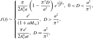 \begin{equation} J(t) \sim \begin{cases} \dfrac {\pi }{2A_1^0a}\left (1 - \dfrac {\pi ^2D}{a^2}\right )e^{\frac {\pi ^2D}{a^2}t},\,\,0\lt D\lt \dfrac {a^2}{\pi ^2}, \\[9pt] \dfrac {e^t}{(1+aM_{\infty })},\,\,D\gt \dfrac {a^2}{\pi ^2}, \\[9pt] \dfrac {\pi e^t}{2A_1^0at},\,\,D=\dfrac {a^2}{\pi ^2}, \end{cases} \end{equation}
as $t\to \infty .$
Thus we have, via (29) and (43), that the solution to (DIVP) has, when
$t\to \infty .$
Thus we have, via (29) and (43), that the solution to (DIVP) has, when $0\lt D\lt a^2/\pi ^2,$
 \begin{equation} u(x,t) = u_s(x) + O(E(t))\,\,\text{as}\,\,t\to \infty , \end{equation}
uniformly for $x\in [0,a]$
, with
$x\in [0,a]$
, with $E(t)$
being exponentially small in
$E(t)$
being exponentially small in $t$
as
$t$
as $t\to \infty .$
Conversely, when
$t\to \infty .$
Conversely, when $D\gt a^2/\pi ^2,$
we have,
$D\gt a^2/\pi ^2,$
we have,
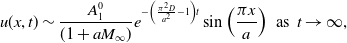 \begin{equation} u(x,t)\sim \frac {A_1^0}{(1+aM_{\infty })}e^{-\left (\frac {\pi ^2D}{a^2}-1\right )t}\sin \left (\frac {\pi x}{a}\right )\,\,\text{as}\,\,t\to \infty , \end{equation}
uniformly for $x\in [0,a]$
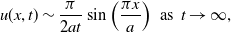
. In the marginal case,
$x\in [0,a]$
. In the marginal case, $D=a^2/\pi ^2,$
we have uniform decay to zero, as in the second case above, but now the decay is slower, being algebraic rather than exponential in
$D=a^2/\pi ^2,$
we have uniform decay to zero, as in the second case above, but now the decay is slower, being algebraic rather than exponential in $t$
, as
$t$
, as $t\to \infty$
, with, specifically,
$t\to \infty$
, with, specifically,
 \begin{equation} u(x,t)\sim \frac {\pi }{2at}\sin \left (\frac {\pi x}{a}\right )\,\,\text{as}\,\,t\to \infty , \end{equation}
uniformly for $x\in [0,a].$
The cases with $0\lt a\le 1/2$
are now complete, and we move on to consider the situation when
$0\lt a\le 1/2$
are now complete, and we move on to consider the situation when $a\gt 1/2.$
2.2.
$a\gt 1/2$

In this subsection, we consider the remaining cases, which have $0\lt D\lt a^2/\pi ^2$
when now
$0\lt D\lt a^2/\pi ^2$
when now $a\gt 1/2.$
Although the scope for direct analytical progress is much more limited in this case, considerable progress can be made in a number of significant asymptotic limits and making useful applications of well-established perturbation methods, and this, complemented and supported by evidence gained from detailed numerical solutions, results in a largely complete overall picture. Details of the numerical methods used to find steady states, compute bifurcation diagrams, solve the evolution problem and calculate eigenvalues for the linear stability problem, which are based on central finite differences and the trapezium rule, are given in Appendix A.
$a\gt 1/2.$
Although the scope for direct analytical progress is much more limited in this case, considerable progress can be made in a number of significant asymptotic limits and making useful applications of well-established perturbation methods, and this, complemented and supported by evidence gained from detailed numerical solutions, results in a largely complete overall picture. Details of the numerical methods used to find steady states, compute bifurcation diagrams, solve the evolution problem and calculate eigenvalues for the linear stability problem, which are based on central finite differences and the trapezium rule, are given in Appendix A.
To begin with, we consider the non-negative and nontrivial steady states which can exist satisfying (1) with (4), (5) and again the Dirichlet boundary conditions (7). This enables us subsequently to draw conclusions concerning the large- $t$
structure of the solution to (DIVP). It is again convenient to consider the steady state structure at fixed
$t$
structure of the solution to (DIVP). It is again convenient to consider the steady state structure at fixed $D$
(as an unfolding parameter) whilst varying
$D$
(as an unfolding parameter) whilst varying $a$
(as a bifurcation parameter). This leads us naturally to consider a number of complementary cases.
$a$
(as a bifurcation parameter). This leads us naturally to consider a number of complementary cases.
2.2.1.
$D\ge 1/4\pi ^2\approx 0.02533$
with
$0\lt (a-\pi \sqrt {D})\ll 1$


In this case, it is again straightforward to prove (via a standard linearisation of the steady form of equation (1) about the trivial equilibrium state) that a steady state transcritical bifurcation from the trivial equilibrium state, as $a$
increases through
$a$
increases through $\pi \sqrt {D}$
, generates a nontrivial, non-negative steady state, and a weakly nonlinear theory is readily developed, which gives this bifurcated steady state the following structure close to the bifurcation point, namely,
$\pi \sqrt {D}$
, generates a nontrivial, non-negative steady state, and a weakly nonlinear theory is readily developed, which gives this bifurcated steady state the following structure close to the bifurcation point, namely,
 \begin{equation} u_s(x;\;a,D) \sim A_b(D)(a-\pi \sqrt {D})\sin \left (\frac {\pi x}{a}\right )\,\,\text{as}\,\,a\to (\pi \sqrt {D})^+, \end{equation}
uniformly for $x\in [0,a]$
(the detailed calculations here are standard, and as such, left for the reader). Here
$x\in [0,a]$
(the detailed calculations here are standard, and as such, left for the reader). Here $A_b(D)$
is a strictly positive
$A_b(D)$
is a strictly positive $O(1)$
constant, independent of
$O(1)$
constant, independent of $a$
.
$a$
.
2.2.2.
$0\lt D\lt 1/4\pi ^2$
with
$0\lt (a-1/2)\ll 1$


It is in this case that we consider whether the unique steady state we have identified in subsection 2.1, which exists for $\pi \sqrt {D}\lt a\le 1/2,$
can be continued into
$\pi \sqrt {D}\lt a\le 1/2,$
can be continued into $a\gt 1/2$
. An examination of the steady state version of equation (1) in the limit as
$a\gt 1/2$
. An examination of the steady state version of equation (1) in the limit as $a\to 1/2$
determines that this continuation is certainly possible, and uniquely so, at least locally, and we perform this as a regular perturbation expansion in integral powers of
$a\to 1/2$
determines that this continuation is certainly possible, and uniquely so, at least locally, and we perform this as a regular perturbation expansion in integral powers of $(a-1/2)$
when
$(a-1/2)$
when $a$
is sufficiently close to 1/2. This results in the following leading order approximation for the continued steady state,
$a$
is sufficiently close to 1/2. This results in the following leading order approximation for the continued steady state,
 \begin{equation} u_s(x;\;a,D) \sim \pi (1-4\pi ^2D)\sin \left (\frac {\pi x}{a}\right ) + O((a-1/2))\,\,\text{as}\,\, a\to \frac {1}{2}^+, \end{equation}
uniformly for $x\in [0,a]$
.
$x\in [0,a]$
.
In the next case, we consider steady states when $D$
is large, with
$D$
is large, with $a=O(\sqrt {D})$
as
$a=O(\sqrt {D})$
as $D\to \infty$
.
$D\to \infty$
.
2.2.3.
$D\gg 1$
with
$a=O(\sqrt {D})$


We write,
 \begin{equation} a = \sqrt {D}\bar {a}, \end{equation}
so that $\bar {a}=O(1)^+$
as
$\bar {a}=O(1)^+$
as $D\to \infty .$
A balancing of terms in the steady state version of equation (1) determines that steady states have
$D\to \infty .$
A balancing of terms in the steady state version of equation (1) determines that steady states have $u_s=O(1)$
as
$u_s=O(1)$
as $D\to \infty$
, after which this nontrivial balance requires us to introduce the scaled coordinate,
$D\to \infty$
, after which this nontrivial balance requires us to introduce the scaled coordinate,
 \begin{equation} \bar {x} = x/\sqrt {D}, \end{equation}
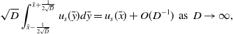
with now $\bar {x}\in [0,\bar {a}]$
. For a steady state, the nonlocal term in (1) becomes (except in passive boundary layers, where
$\bar {x}\in [0,\bar {a}]$
. For a steady state, the nonlocal term in (1) becomes (except in passive boundary layers, where $\bar {x}=O(1/\sqrt {D})^+ \text{or}\, \bar {x}= \bar {a}-O(1/\sqrt {D})^+$
),
$\bar {x}=O(1/\sqrt {D})^+ \text{or}\, \bar {x}= \bar {a}-O(1/\sqrt {D})^+$
),
 \begin{equation} \sqrt {D}\int _{\bar {x}-\frac {1}{2\sqrt {D}}}^{\bar {x}+\frac {1}{2\sqrt {D}}}{u_s(\bar {y})}d\bar {y} = u_s(\bar {x}) + O(D^{-1})\,\,\text{as}\,\,D\to \infty , \end{equation}
with $\bar {x}\in (O(1/\sqrt {D})^+, \bar {a}-O(1/\sqrt {D})^+).$
A steady state
$\bar {x}\in (O(1/\sqrt {D})^+, \bar {a}-O(1/\sqrt {D})^+).$
A steady state $u_s\;:\;[0,\bar {a}]\to \mathbb{R}$
is now expanded in the asymptotic form,
$u_s\;:\;[0,\bar {a}]\to \mathbb{R}$
is now expanded in the asymptotic form,
 \begin{equation} u_s(\bar {x},\bar {a};\;D) = U_s(\bar {x},\bar {a}) + O(D^{-1})\,\,as\,\,D\to \infty , \end{equation}
with $\bar {x}\in [0,\bar {a}]$
. On substitution from expansion (52) into equation (1) (when written in terms of the coordinate
$\bar {x}\in [0,\bar {a}]$
. On substitution from expansion (52) into equation (1) (when written in terms of the coordinate $\bar {x}$
), we obtain at leading order the local, nonlinear ODE for
$\bar {x}$
), we obtain at leading order the local, nonlinear ODE for $U_s$
,
$U_s$
,
 \begin{equation} U_s'' + U_s(1-U_s) = 0,\,\,\bar {x}\in (0,\bar {a}), \end{equation}
where $'=d/d\bar {x}$
. We note that this is precisely the Dirichlet problem for steady states on the interval
$'=d/d\bar {x}$
. We note that this is precisely the Dirichlet problem for steady states on the interval $[0,\bar {a}]$
for the local Fisher-KPP equation (see, for example, [Reference Fife9]). This is to be solved subject to the boundary and non-negativity conditions,
$[0,\bar {a}]$
for the local Fisher-KPP equation (see, for example, [Reference Fife9]). This is to be solved subject to the boundary and non-negativity conditions,
 \begin{equation} U_s(0,\bar {a})=U_s(\bar {a},\bar {a})=0\,\,,\,\,U_s(\bar {x},\bar {a})\ge 0\,\,\forall \,\,\bar {x}\in [0,\bar {a}]. \end{equation}
It is straightforward to consider solutions to this nonlinear boundary value problem by recasting it in the $(U_s,U_s')$
phase plane. We omit details, which can be readily confirmed by the reader, and simply record the conclusions. Firstly, it has no nontrivial solutions when
$(U_s,U_s')$
phase plane. We omit details, which can be readily confirmed by the reader, and simply record the conclusions. Firstly, it has no nontrivial solutions when $0\lt \bar {a}\le \pi$
. However, consistent with the earlier theory, a transcritical bifurcation from the trivial solution occurs as
$0\lt \bar {a}\le \pi$
. However, consistent with the earlier theory, a transcritical bifurcation from the trivial solution occurs as $\bar {a}$
increases through the bifurcation value
$\bar {a}$
increases through the bifurcation value $\bar {a}=\pi$
(this being, in term of
$\bar {a}=\pi$
(this being, in term of $a$
, the value
$a$
, the value $a=\pi \sqrt {D},$
consistent with the earlier theory). This bifurcation produces a unique nontrivial solution in
$a=\pi \sqrt {D},$
consistent with the earlier theory). This bifurcation produces a unique nontrivial solution in $\bar {a}\gt \pi .$
We denote this solution by
$\bar {a}\gt \pi .$
We denote this solution by $U_s=\nu (\bar {x},\bar {a})$
with
$U_s=\nu (\bar {x},\bar {a})$
with $\bar {x}\in [0,\bar {a}]$
, and it has the following key properties,
$\bar {x}\in [0,\bar {a}]$
, and it has the following key properties,
-
1.
$\nu (\bar {x},\bar {a})\gt 0\,\,\forall \,\,\bar {x}\in (0,\bar {a}),$
-
2.
$\nu (\bar {x},\bar {a})$
is symmetric about
$\bar {x}=\frac {1}{2}\bar {a},$
-
3.
$\nu (\bar {x},\bar {a})$
has a single turning point, which is a maximum, at
$\bar {x}=\frac {1}{2}\bar {a}$
, -
4. with
$A(\bar {a})=\text{sup}_{\bar {x}\in [0,\bar {a}]}(\nu (\bar {x},\bar {a}))$
, then
$A(\bar {a})$
is monotone increasing with
$\bar {a}\gt \pi$
, and
$A(\bar {a})\to 0$
as
$\bar {a}\to \pi$
, whilst
$A(\bar {a})\to 1$
as
$\bar {a}\to \infty .$


It is also straightforward to develop the following formal asymptotic approximations for the nontrivial steady state; the regular perturbation,
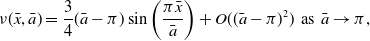 \begin{equation} \nu (\bar {x},\bar {a}) = \frac {3}{4}(\bar {a}-\pi )\sin \left (\frac {\pi \bar {x}}{\bar {a}}\right )+O((\bar {a}-\pi )^2)\,\,\text{as}\,\,\bar {a}\to \pi , \end{equation}
uniformly for $\bar {x}\in [0,\bar {a}],$
and the matched asymptotic approximation,
$\bar {x}\in [0,\bar {a}],$
and the matched asymptotic approximation,
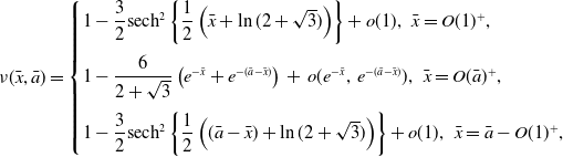 \begin{equation} \nu (\bar {x},\bar {a}) = \begin{cases} 1 - \dfrac {3}{2}\text{sech}^2 \left \{\dfrac {1}{2}\left (\bar {x}+\ln {(2+\sqrt {3})}\right )\right \}+o(1),\,\,\bar {x}=O(1)^+,\\[12pt] 1 - \dfrac {6}{2+\sqrt {3}}\left ( e^{-\bar {x}} + e^{-(\bar {a}-\bar {x})}\right )\,+\,o(e^{-\bar {x}},\,e^{-(\bar {a}-\bar {x})}),\,\,\bar {x}=O(\bar {a})^+,\\[12pt] 1 - \dfrac {3}{2}\text{sech}^2\left \{\dfrac {1}{2}\left ((\bar {a}-\bar {x})+\ln {(2+\sqrt {3})}\right )\right \}+o(1),\,\,\bar {x}=\bar {a}-O(1)^+, \end{cases} \end{equation}
as $\bar {a}\to \infty .$
We see that the structure of the steady state changes from a weakly nonlinear sinusoidal hump close to its appearance at the local bifurcation when
$\bar {a}\to \infty .$
We see that the structure of the steady state changes from a weakly nonlinear sinusoidal hump close to its appearance at the local bifurcation when $\overline {a} = \pi$
to an almost uniformly (except in thin boundary layers) flat profile across the interval when
$\overline {a} = \pi$
to an almost uniformly (except in thin boundary layers) flat profile across the interval when $\overline {a}$
becomes large. This concludes the analysis for
$\overline {a}$
becomes large. This concludes the analysis for $D$
large with
$D$
large with $a=O(\sqrt {D}),$
and the asymptotic analysis has shown that there are no non-negative nontrivial steady states for
$a=O(\sqrt {D}),$
and the asymptotic analysis has shown that there are no non-negative nontrivial steady states for $0\lt a\le \pi \sqrt {D}$
, but a unique such steady state at each
$0\lt a\le \pi \sqrt {D}$
, but a unique such steady state at each $a\gt \pi \sqrt {D}.$
The next case has $D$
of
$D$
of $O(1)$
with
$O(1)$
with $a$
large.
$a$
large.
2.2.4.
$0\lt D\le O(1)$
with
$a\gg 1$


In this case, since the domain length $a$
is large, whilst
$a$
is large, whilst $D$
remains of O(1), we expect that there will be symmetric boundary layers when
$D$
remains of O(1), we expect that there will be symmetric boundary layers when $x=O(1)^+$
and
$x=O(1)^+$
and $x=a-O(1)^+$
as
$x=a-O(1)^+$
as $a\to \infty$
, at either end of a bulk region separating these two boundary layers. We also expect that any nontrivial steady state will have
$a\to \infty$
, at either end of a bulk region separating these two boundary layers. We also expect that any nontrivial steady state will have $u_s=O(1)$
in the bulk region and in the boundary layers, as
$u_s=O(1)$
in the bulk region and in the boundary layers, as $a\to \infty$
. Therefore, it is natural to pursue an analysis of this case via the method of matched asymptotic expansions (see, for example, [Reference Miller14], chapter 8). It is instructive to begin in the boundary layers, and as these are symmetric, we need only consider the boundary layer at the left end of the domain. In this boundary layer, we expand as,
$a\to \infty$
. Therefore, it is natural to pursue an analysis of this case via the method of matched asymptotic expansions (see, for example, [Reference Miller14], chapter 8). It is instructive to begin in the boundary layers, and as these are symmetric, we need only consider the boundary layer at the left end of the domain. In this boundary layer, we expand as,
 \begin{equation} u_s(x,D,a) \sim U_b(x,D)\,\,\text{as}\,\,a\to \infty , \end{equation}
with $x=O(1)^+.$
The leading order problem is then readily obtained from substitution of (57) into equation (1) as,
$x=O(1)^+.$
The leading order problem is then readily obtained from substitution of (57) into equation (1) as,
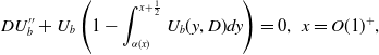 \begin{equation} DU_b'' + U_b\left (1 - \int _{\alpha (x)}^{x+\frac {1}{2}}{U_b(y,D)}dy\right ) = 0,\,\,x=O(1)^+, \end{equation}
with $U_b$
being non-negative, and subject to the boundary conditions,
$U_b$
being non-negative, and subject to the boundary conditions,
 \begin{equation} U_b(0,D)=0\,\,\text{and}\,\,U_b(x,D) \,\text{bounded as}\,\,x\to \infty . \end{equation}
This nonlocal boundary value problem depends only upon the parameter $D$
, and we have performed a systematic numerical study using a standard shooting method, together with a linearised analysis at large
$D$
, and we have performed a systematic numerical study using a standard shooting method, together with a linearised analysis at large $x$
to refine this. For convenience, we refer to this nonlocal boundary value problem as (SIBP), and the numerical analysis, together with the linearised theory (which are straightforward and, for brevity, need not be detailed here), determine the following key properties:
$x$
to refine this. For convenience, we refer to this nonlocal boundary value problem as (SIBP), and the numerical analysis, together with the linearised theory (which are straightforward and, for brevity, need not be detailed here), determine the following key properties:
-
1. For each
$D\ge \Delta _1\approx 0.00297$
(see (NB1), section 4), the numerical shooting method determines that (SIBP) has a single solution. The linearised theory then determines that this solution has
$U_b(x,D)\to 1$
, exponentially in
$x$
, as
$x\to \infty$
. In addition, it determines that
$U_b(x,D)$
is monotone when
$D\ge \Delta _m$
, but has harmonic exponential decay to unity when
$\Delta _1\lt D\lt \Delta _m$
, with the exponential decay rate reducing to zero as
$D\to \Delta _1$
. Here
$\Delta _m=2 l^{-3}\sinh \left (\frac {1}{2}l\right )$
, with
$l \approx 5.9694$
being the unique positive solution to the algebraic equation
$6\tanh \left (\frac {1}{2}l\right ) = l$
. This determines
$\Delta _m \approx 0.0928$
. -
2. For each
$0\lt D\lt \Delta _1$
, the numerical shooting method now confirms that (SIBP) has a one-parameter family of solutions, parameterised by a characteristic wavelength
$\lambda$
, with
$\lambda \in (\lambda _1^-(D),\lambda _1^+(D))$
, where the notation here is as introduced in section 3 and section 4 of (NB1). Specifically, each of these solutions is now asymptotic to a steady non-negative, periodic solution of (1), oscillating about unity, and with wavelength
$\lambda$
, as
$x\to \infty$
. In particular,(60)Here
\begin{equation} U_b(x,D)\sim F_p(x - x_b(\lambda ,D),\lambda ,D)\,\,\text{as}\,\,x\to \infty . \end{equation}
$F_p(y,\lambda ,D)$
, for
$y\in [0,\lambda )$
and
$(\lambda ,D)\in \Omega _1$
, is readily identified with that nontrivial, non-negative periodic steady state, with wavelength
$\lambda$
, and oscillating about unity, as introduced and analysed in detail in section 4 of (NB1), with the spatial translation invarience fixed so that
$F_p(0,\lambda ,D)=1\,\,\text{and}\,\, F_p'(0,\lambda ,D)\gt 0$
. In addition,
$x_b(\lambda ,D)$
is a shift of origin, which is determined in the solution of (SIBP), and can be estimated numerically when necessary.


This completes the structure in the left boundary layer. In the right boundary layer, we have, symmetrically,
 \begin{equation} u_s(x,D,a)\sim U_b(a-x,D)\,\,\text{as}\,\,a\to \infty , \end{equation}
with $x=a-O(1)^+$
. We must now connect the two boundary layers through the bulk region, when
$x=a-O(1)^+$
. We must now connect the two boundary layers through the bulk region, when $x\in (O(1)^+, a-O(1)^+)$
. The situation for
$x\in (O(1)^+, a-O(1)^+)$
. The situation for $D\ge \Delta _1$
is straightforward. In the bulk region, asymptotic matching with the solution in the left and right boundary layers (via item (1) above, and (61), using the classical Van Dyke asymptotic matching principle, [Reference Van Dyke18]) dictates that in equation (1), we must simply take,
$D\ge \Delta _1$
is straightforward. In the bulk region, asymptotic matching with the solution in the left and right boundary layers (via item (1) above, and (61), using the classical Van Dyke asymptotic matching principle, [Reference Van Dyke18]) dictates that in equation (1), we must simply take,
 \begin{equation} u_s(x,D,a) \sim 1 \,\,\text{as}\,\,a\to \infty , \end{equation}
for $x\in (O(1)^+,a-O(1)^+)$
, and the structure is complete.
$x\in (O(1)^+,a-O(1)^+)$
, and the structure is complete.
For $0\lt D\lt \Delta _1$
, the situation is more complicated due to the changing structure in the right and left boundary layers (as recorded in item (2) above) and we begin by recalling from (NB1) (see section 4) the following general properties of
$0\lt D\lt \Delta _1$
, the situation is more complicated due to the changing structure in the right and left boundary layers (as recorded in item (2) above) and we begin by recalling from (NB1) (see section 4) the following general properties of $F_p(x,\lambda ,D)$
with
$F_p(x,\lambda ,D)$
with $x\in \mathbb{R}$
:
$x\in \mathbb{R}$
:
-
•
$F_p(x,\lambda ,D)$
has exactly one maximum point and one minimum point, and no other stationary points, over one wavelength
$\lambda$
-
• Consecutive maximum and minimum points are separated by a distance
$\frac {1}{2}\lambda$
. -
•
$F_p(x,\lambda ,D)$
is an even function about each of its stationary points.


Now let $x=x_M(\lambda ,D)$
be the location of the first maximum point of
$x=x_M(\lambda ,D)$
be the location of the first maximum point of $F_p(x,\lambda ,D)$
on the positive
$F_p(x,\lambda ,D)$
on the positive $x$
-axis. Using the above properties, we can conclude for each
$x$
-axis. Using the above properties, we can conclude for each $r\in \mathbb{N}$
,
$r\in \mathbb{N}$
, $D\in (0,\Delta _1)$
and
$D\in (0,\Delta _1)$
and $\lambda \in (\lambda _1^+(D),\lambda _1^-(D))$
(see (NB1), section 4, for this notation) that the function
$\lambda \in (\lambda _1^+(D),\lambda _1^-(D))$
(see (NB1), section 4, for this notation) that the function $F_p(x-x_b(\lambda ,D),\lambda ,D)$
has a stationary point at the positive location
$F_p(x-x_b(\lambda ,D),\lambda ,D)$
has a stationary point at the positive location
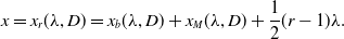 \begin{equation} x = x_r(\lambda ,D) = x_b(\lambda ,D) + x_M(\lambda ,D) +\frac {1}{2}(r-1)\lambda . \end{equation}
Therefore, following the final property above, we conclude that $F_p(x-x_b(\lambda ,D),\lambda ,D)$
:
$F_p(x-x_b(\lambda ,D),\lambda ,D)$
:
-
• is an even function of
$x$
about
$x=x_r(\lambda ,D)$
, -
• has a maximum or minimum point at this location when
$r$
is odd or even, respectively, -
• has exactly
$r$
maximum points for
$x\in [0,2x_r(\lambda ,D)]$
.


With this information in hand, we can now return to the bulk region. First, fix $D\in (0,\Delta _1)$
, and choose
$D\in (0,\Delta _1)$
, and choose $r\in \mathbb{N}$
with
$r\in \mathbb{N}$
with $r$
large. Then for each
$r$
large. Then for each $\lambda \in (\lambda _1^-(D),\lambda _1^+(D))$
, take,
$\lambda \in (\lambda _1^-(D),\lambda _1^+(D))$
, take,
 \begin{equation} a = 2x_r(\lambda ,D) = \lambda (r-1) + O(1)\,\,\text{as}\,\,r\to \infty . \end{equation}
For this large value of $a$
, as
$a$
, as $r\to \infty$
, we then take,
$r\to \infty$
, we then take,
 \begin{equation} u_s(x,D,a) \sim F_p(x-x_b(\lambda ,D),\lambda ,D) \end{equation}
for $x\in (O(1)^+,a-O(1)^+)$
. We observe, via (64) and the first comment above, that the asymptotic approximation (65) asymptotically matches (again according to the Van Dyke matching principle) with the asymptotic approximations in the boundary layers (57) and (61) when
$x\in (O(1)^+,a-O(1)^+)$
. We observe, via (64) and the first comment above, that the asymptotic approximation (65) asymptotically matches (again according to the Van Dyke matching principle) with the asymptotic approximations in the boundary layers (57) and (61) when $x=O(1)^+$
and
$x=O(1)^+$
and $x=a-O(1)^+$
, respectively. Thus, to summarise, for each fixed
$x=a-O(1)^+$
, respectively. Thus, to summarise, for each fixed $0\lt D\lt \Delta _1$
, we have shown, for each large natural number
$0\lt D\lt \Delta _1$
, we have shown, for each large natural number $r$
, and then each
$r$
, and then each
 \begin{equation} a \in (\lambda _1^-(D)(r-1)+O(1)^+, \lambda _1^+(D)(r-1)+O(1)^+) \equiv I_r(D), \end{equation}
that a nontrivial, non-negative steady state exists and we have constructed its form. Away from boundary layers at the ends of the long domain, this steady state is periodic about unity, with wavelength (for $a=O(r)$
as given in (66))
$a=O(r)$
as given in (66))
 \begin{equation} \lambda \sim a(r-1)^{-1}, \end{equation}
and having $r$
peak points across the domain. To characterise each such steady state it is instructive to measure its norm in
$r$
peak points across the domain. To characterise each such steady state it is instructive to measure its norm in $L^1$
. Firstly, for
$L^1$
. Firstly, for $0\lt D\lt \Delta _1$
and
$0\lt D\lt \Delta _1$
and $\lambda \in (\lambda _1^-(D),\lambda _1^+(D))$
, we write, over an interval of one wavelength
$\lambda \in (\lambda _1^-(D),\lambda _1^+(D))$
, we write, over an interval of one wavelength $\lambda$
,
$\lambda$
,
 \begin{equation} A(\lambda ,D) = || F_p(\cdot ,\lambda ,D)||_1 \equiv \int _0^\lambda {F_p(y,\lambda ,D)}dy, \end{equation}
and numerically determined contour plots of $A(\lambda ,D)$
in the
$A(\lambda ,D)$
in the $(D,\lambda )$
plane, for each of the first four tongues where the periodic steady states exist (see (NB1), section 4 for this notation and terminology), are shown in Figure 2. Outside the tongues,
$(D,\lambda )$
plane, for each of the first four tongues where the periodic steady states exist (see (NB1), section 4 for this notation and terminology), are shown in Figure 2. Outside the tongues, $A$
varies linearly with
$A$
varies linearly with $\lambda$
as we have plotted the result for the equilibrium solution,
$\lambda$
as we have plotted the result for the equilibrium solution, $u_e=1$
. Within the tongues, the deviation of
$u_e=1$
. Within the tongues, the deviation of $A$
from this linear behaviour becomes stronger as
$A$
from this linear behaviour becomes stronger as $D$
decreases, becoming independent of
$D$
decreases, becoming independent of $\lambda$
as
$\lambda$
as $D \to 0$
. The qualitative behaviour of
$D \to 0$
. The qualitative behaviour of $A(\lambda ,D)$
is very similar in each tongue.
$A(\lambda ,D)$
is very similar in each tongue.
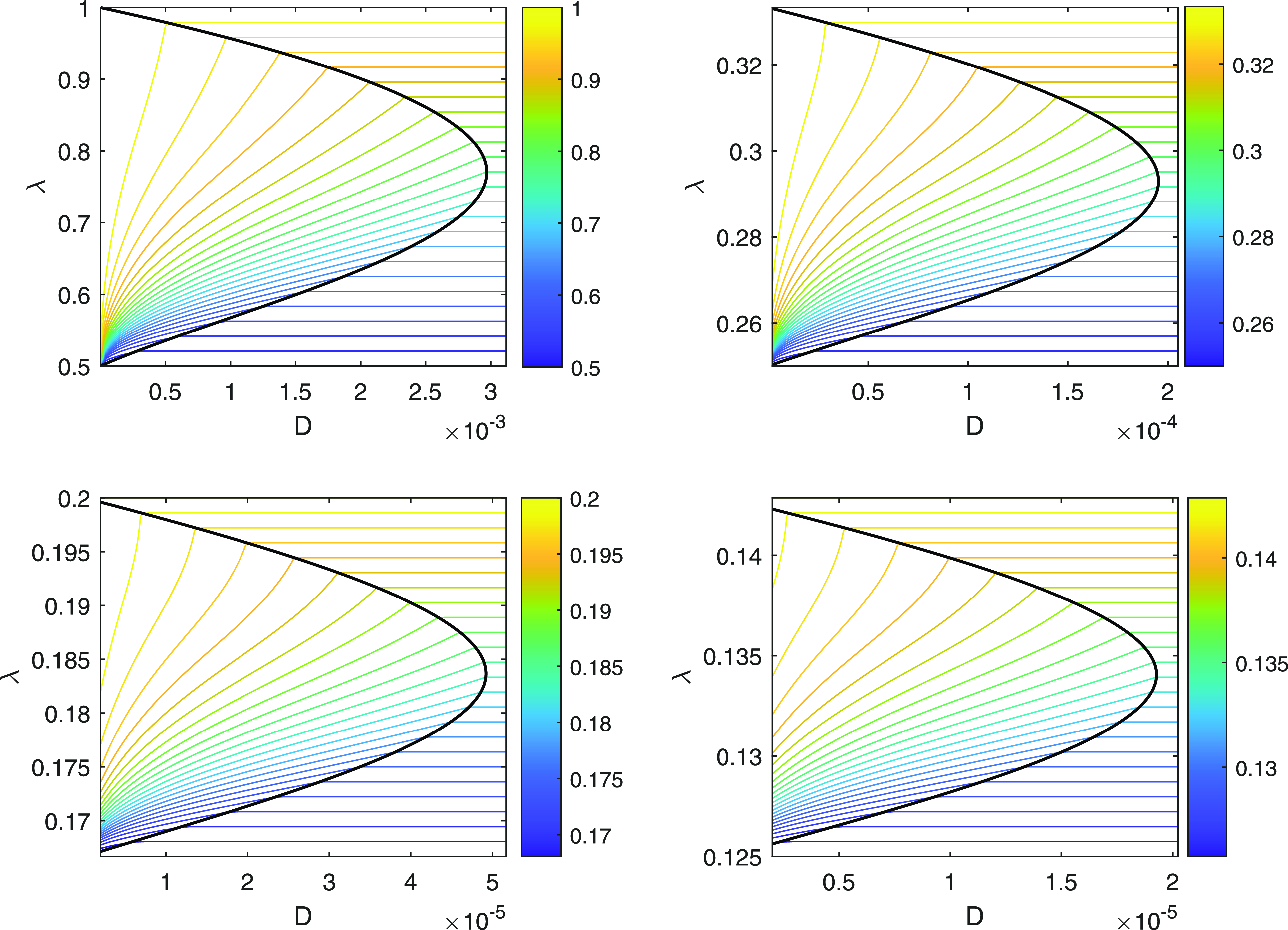
Figure 2. The $L^1$
norm,
$L^1$
norm, $A(\lambda ,D)$
, of the nontrivial, non-negative, periodic steady states identified in (NB1). The first four tongue regions are shown in the
$A(\lambda ,D)$
, of the nontrivial, non-negative, periodic steady states identified in (NB1). The first four tongue regions are shown in the $(D,\lambda )$
plane.
$(D,\lambda )$
plane.
It is now straightforward to determine, via construction and using $A(\lambda ,D)$
in the first tongue, that for fixed
$A(\lambda ,D)$
in the first tongue, that for fixed $D$
, and given large
$D$
, and given large $r$
, then,
$r$
, then,
 \begin{equation} ||u_s(\cdot ,D,a)||_1 \sim rA(a(r-1)^{-1},D)\,\,\forall \,\,a\in ((r-1)\lambda _1^-(D),(r-1)\lambda _1^+(D)). \end{equation}
With $D$
fixed and
$D$
fixed and $r$
large, we consider the
$r$
large, we consider the $(a,||u_s(\cdot ,D,a)||_1)$
bifurcation diagram when
$(a,||u_s(\cdot ,D,a)||_1)$
bifurcation diagram when $a$
is large; we have now shown above that each interval with
$a$
is large; we have now shown above that each interval with $a\in I_r(D)$
, containing the branch of
$a\in I_r(D)$
, containing the branch of $r$
-peak steady states, has an echelon overlap with its predecessor when
$r$
-peak steady states, has an echelon overlap with its predecessor when $a\in I_{r-1}(D)$
, containing the branch of
$a\in I_{r-1}(D)$
, containing the branch of $(r-1)$
-peak steady states, and this structure continues as
$(r-1)$
-peak steady states, and this structure continues as $r$
increases, with the number of overlaps, with previous echelons, increasing linearly with increasing
$r$
increases, with the number of overlaps, with previous echelons, increasing linearly with increasing $r$
. This can be represented on the
$r$
. This can be represented on the $(a,||u_s(\cdot ,D,a)||_1)$
bifurcation plane as follows: for each large
$(a,||u_s(\cdot ,D,a)||_1)$
bifurcation plane as follows: for each large $r$
, the associated
$r$
, the associated $r$
-peak branch of steady states has a graph given by (69) on this plane. The graphs of these branches form a lifting, and multiply overlapping, echelon of separate segments. At a given large
$r$
-peak branch of steady states has a graph given by (69) on this plane. The graphs of these branches form a lifting, and multiply overlapping, echelon of separate segments. At a given large $a$
, the overlapping echelons are associated with those natural numbers
$a$
, the overlapping echelons are associated with those natural numbers $r_m(a,D)\le r\le r_M(a,D)$
, where
$r_m(a,D)\le r\le r_M(a,D)$
, where
 \begin{equation} r_m(a,D) \sim \frac {a}{\lambda _1^+(D)} + 1, \end{equation}
 \begin{equation} r_M(a,D) \sim \frac {a}{\lambda _1^-(D)} + 1, \end{equation}
as $a\to \infty$
. Each segment has a base length increasing linearly with
$a\to \infty$
. Each segment has a base length increasing linearly with $r$
, a slope of O(1) and a consequent
$r$
, a slope of O(1) and a consequent $O(r)$
increase in norm on traversing the segment. In addition, each segment is lifted by an
$O(r)$
increase in norm on traversing the segment. In addition, each segment is lifted by an $O(1)$
value each time
$O(1)$
value each time $r$
is increased by unity. Careful numerical solution of the full boundary value problem, using pseudo-arclength continuation in the
$r$
is increased by unity. Careful numerical solution of the full boundary value problem, using pseudo-arclength continuation in the $(a, ||u_s||_1)$
-plane, reveals that each two consecutive, overlapping, branches in the echelon are continuously connected by a hanging, elongated loop with two facing saddle-node bifurcations, as illustrated in Figure 3. On the lower part of this loop, the associated steady state develops an additional peak through a rapid process, which occurs, for
$(a, ||u_s||_1)$
-plane, reveals that each two consecutive, overlapping, branches in the echelon are continuously connected by a hanging, elongated loop with two facing saddle-node bifurcations, as illustrated in Figure 3. On the lower part of this loop, the associated steady state develops an additional peak through a rapid process, which occurs, for $r$
large, in the neighbourhood of the stationary point at
$r$
large, in the neighbourhood of the stationary point at $x=\frac {1}{2}a$
, in the bulk region, and allows this central stationary point to flip through itself. There is then a rapid transition to the associated multi-peak steady state as each respective saddle-node bifurcation is traversed. A typical case is shown in Figure 4.
$x=\frac {1}{2}a$
, in the bulk region, and allows this central stationary point to flip through itself. There is then a rapid transition to the associated multi-peak steady state as each respective saddle-node bifurcation is traversed. A typical case is shown in Figure 4.
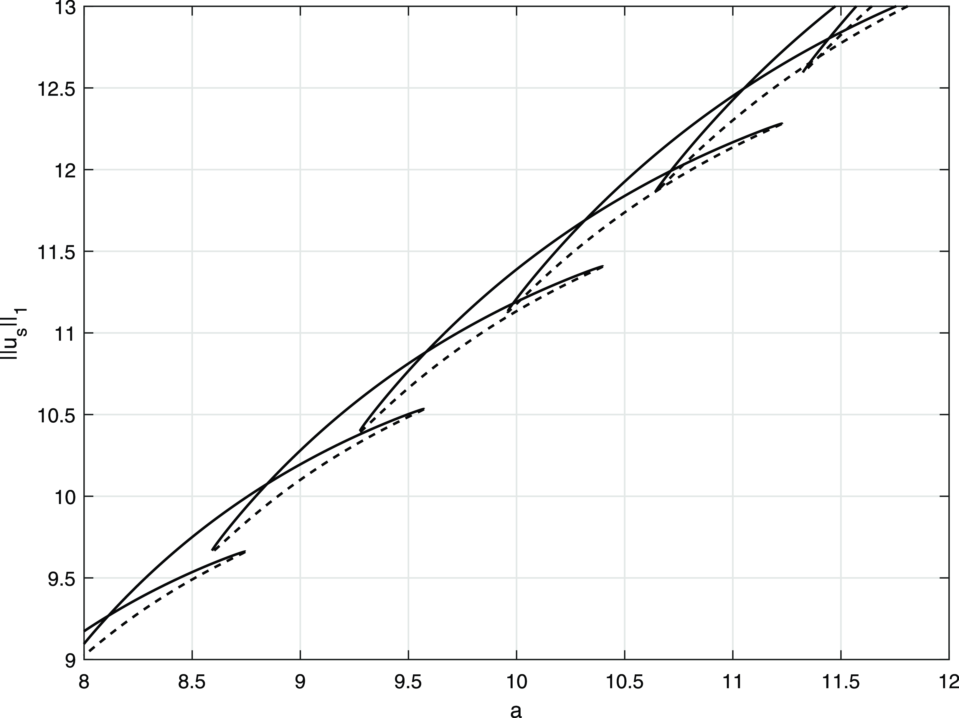
Figure 3. Part of the $(a,||u_s||_1)$
bifurcation diagram, when
$(a,||u_s||_1)$
bifurcation diagram, when $D = 2 \times 10^{-3}$
. Unstable branches of steady states are indicated by broken lines.
$D = 2 \times 10^{-3}$
. Unstable branches of steady states are indicated by broken lines.
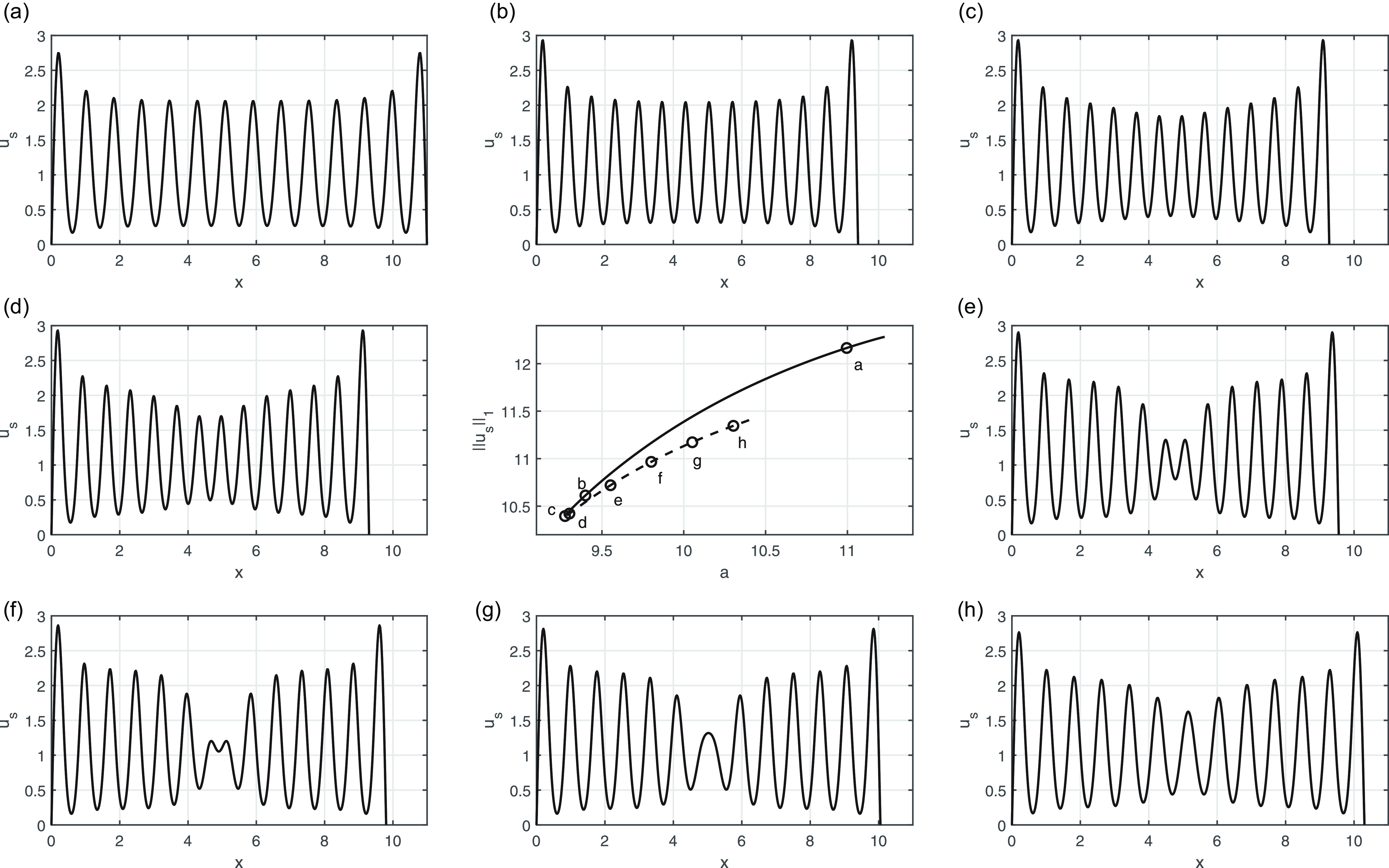
Figure 4. The profile of the steady state $u_s$
, with
$u_s$
, with $D=2\times 10^{-3}$
, as the
$D=2\times 10^{-3}$
, as the $r=14$
to
$r=14$
to $r=13$
echelon of the bifurcation diagram is traversed. The central panel shows the relevant portion of the bifurcation diagram. Note the different
$r=13$
echelon of the bifurcation diagram is traversed. The central panel shows the relevant portion of the bifurcation diagram. Note the different $u_s$
-axis range in the other panels, individually labelled (a) to (h), and identified on the central panel. Also, only the steady states (a) to (c), on the upper echelon, are stable, with the steady states (d) to (h), on the connecting loop, each being unstable.
$u_s$
-axis range in the other panels, individually labelled (a) to (h), and identified on the central panel. Also, only the steady states (a) to (c), on the upper echelon, are stable, with the steady states (d) to (h), on the connecting loop, each being unstable.
The above large- $a$
structure continues to hold as
$a$
structure continues to hold as $D$
becomes small. However, when
$D$
becomes small. However, when $D$
is small, we can take advantage of the approximations to
$D$
is small, we can take advantage of the approximations to $F_p(x,\lambda ,D)$
as detailed in section 4 of (NB1). In particular, we have, as
$F_p(x,\lambda ,D)$
as detailed in section 4 of (NB1). In particular, we have, as $D\to 0$
,
$D\to 0$
,
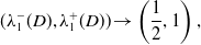 \begin{equation} (\lambda _1^-(D),\lambda _1^+(D))\to \left (\frac {1}{2},1\right ), \end{equation}
 \begin{equation} x_b(\lambda ,D) + x_M(\lambda ,D) \to \frac {1}{2}\left (\lambda -\frac {1}{2}\right )\,\,\forall \,\,\lambda \in \left (\frac {1}{2}+O(\sqrt {D}),1-O(D)\right ), \end{equation}
and
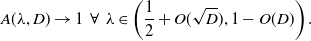 \begin{equation} A(\lambda ,D)\to 1\,\,\forall \,\,\lambda \in \left (\frac {1}{2}+O(\sqrt {D}),1-O(D)\right ). \end{equation}
This completes the examination of the steady state structure to (DIVP) when $a$
is large.
$a$
is large.
We now continue by considering the steady state structure when $D$
is small and
$D$
is small and $a\gt 1/2 + o(1)^+$
as
$a\gt 1/2 + o(1)^+$
as $D\to 0$
.
$D\to 0$
.
2.2.5.
$0\lt D\ll 1$
with
$a\gt 1/2 + o(1)$
as
$D\to 0$


In this case, to again avoid extensive repetition, we take advantage of the detailed theory developed in subsection $4.1$
of (NB1) for the periodic steady states
$4.1$
of (NB1) for the periodic steady states $F_p(x,\lambda ,D)$
with
$F_p(x,\lambda ,D)$
with $\lambda \in (\lambda _1^-(D),\lambda _1^+(D))$
, now directly using the terminology laid out in (NB1) in subsection
$\lambda \in (\lambda _1^-(D),\lambda _1^+(D))$
, now directly using the terminology laid out in (NB1) in subsection $4.1$
. Summarising from (NB1), the family of nontrivial and non-negative periodic states are given by (at leading order as
$4.1$
. Summarising from (NB1), the family of nontrivial and non-negative periodic states are given by (at leading order as $D\to 0$
, and noting that a passive edge region, of thickness
$D\to 0$
, and noting that a passive edge region, of thickness $O(D^{\frac {1}{4}})$
, is present at the end of the supported leading order form for
$O(D^{\frac {1}{4}})$
, is present at the end of the supported leading order form for $F_p$
, which provides local smoothing to the gradient discontinuity in the leading order form), for each wavelength
$F_p$
, which provides local smoothing to the gradient discontinuity in the leading order form), for each wavelength $\lambda \in (1/2 + O(D^{\frac {1}{2}})^+, 1-O(D)^+)$
, the asymptotic approximation,
$\lambda \in (1/2 + O(D^{\frac {1}{2}})^+, 1-O(D)^+)$
, the asymptotic approximation,
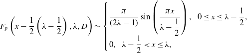 \begin{equation} F_p\left (x - \dfrac {1}{2}\left (\lambda -\dfrac {1}{2}\right ),\lambda ,D\right ) \sim \begin{cases} \dfrac {\pi }{(2\lambda -1)}\sin \left (\dfrac {\pi x}{\lambda -\dfrac {1}{2}}\right ),\,\,\, 0\le x \le \lambda -\dfrac {1}{2}, \\[5pt] 0,\,\,\,\lambda -\dfrac {1}{2} \lt x \le \lambda , \end{cases} \end{equation}
as $D\to 0$
with
$D\to 0$
with $x\in [0,\lambda ]$
. We also recall from (NB1) (equation
$x\in [0,\lambda ]$
. We also recall from (NB1) (equation $(126)$
), and using the notation (68), that
$(126)$
), and using the notation (68), that
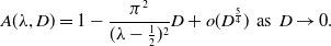 \begin{equation} A(\lambda ,D) = 1 - \frac {\pi ^2}{(\lambda -\frac {1}{2})^2}D + o(D^{\frac {5}{4}})\,\,\text{as}\,\,D\to 0. \end{equation}
with $\lambda \in (1/2+O(D^{\frac {1}{2}})^+,1-O(D)^+)$
. Now, for each
$\lambda \in (1/2+O(D^{\frac {1}{2}})^+,1-O(D)^+)$
. Now, for each $r=2,3,4\ldots$
, we can construct from (75) (by periodic glueing) an
$r=2,3,4\ldots$
, we can construct from (75) (by periodic glueing) an $r$
-peak steady state at each domain size
$r$
-peak steady state at each domain size $a$
with
$a$
with
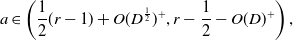 \begin{equation} a \in \left (\frac {1}{2}(r-1) + O(D^{\frac {1}{2}})^+,r-\frac {1}{2}-O(D)^+\right ), \end{equation}
which is given by
 \begin{equation} u_s(x,D,a) \sim F_p\left (x - \frac {1}{2}\left (\lambda (a,r)-\frac {1}{2}\right ),\left (a+\frac {1}{2}\right )r^{-1},D\right )\,\,\text{as}\,\,D\to 0, \end{equation}
for $x\in [0,a]$
, and
$x\in [0,a]$
, and $F_p$
approximated as in (75), with
$F_p$
approximated as in (75), with
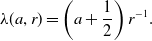 \begin{equation} \lambda (a,r)=\left (a+\frac {1}{2}\right )r^{-1}. \end{equation}
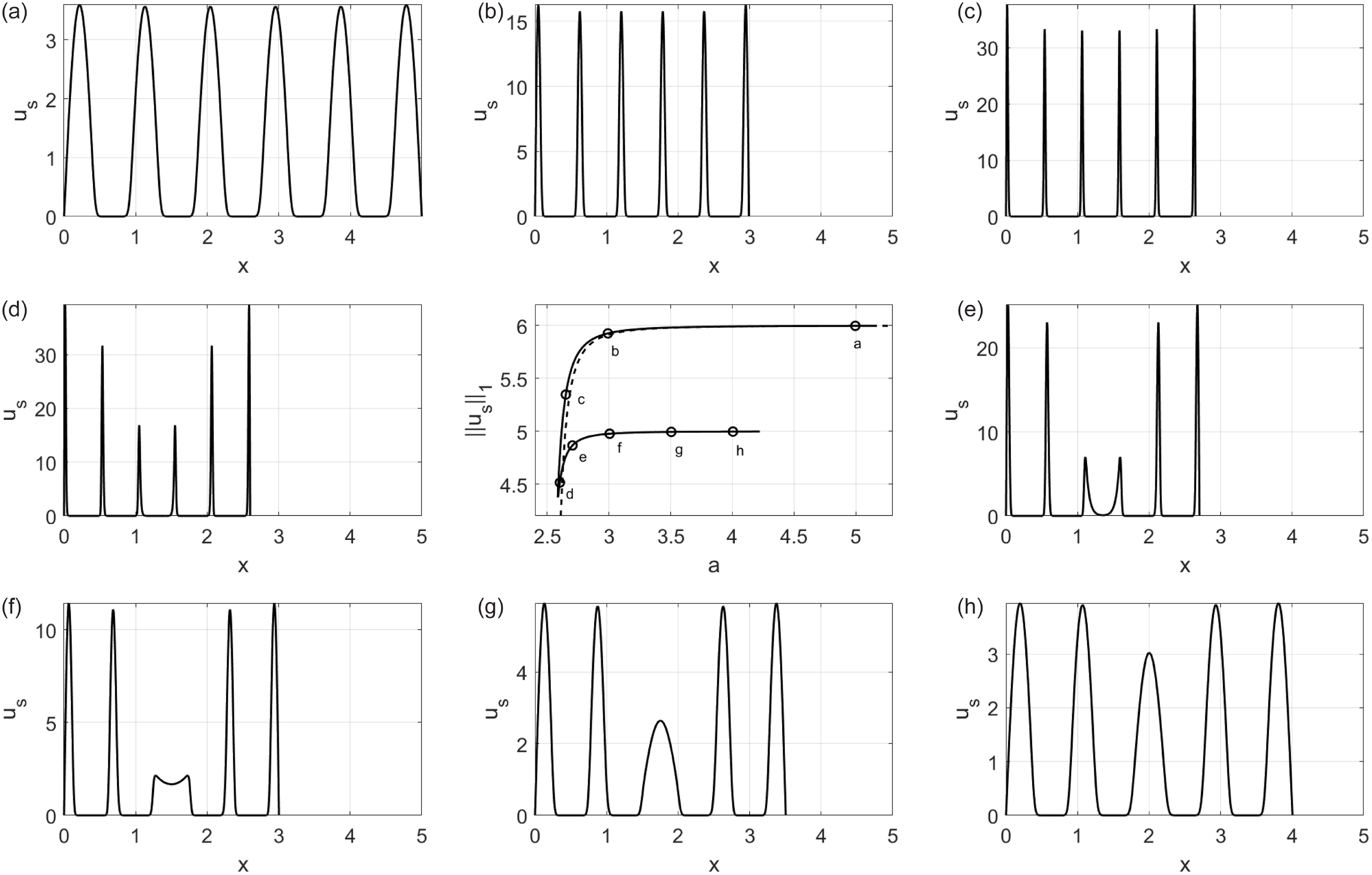
Figure 5. The profile of the steady state $u_s$
as the
$u_s$
as the $r=6$
to
$r=6$
to $r=5$
echelon of the bifurcation diagram is traversed. The central panel shows the relevant portion of the bifurcation diagram, with the broken line given by (80). Note the different
$r=5$
echelon of the bifurcation diagram is traversed. The central panel shows the relevant portion of the bifurcation diagram, with the broken line given by (80). Note the different $u_s$
-axis limits in the other panels, individually labelled (a) to (h), and identified on the central panel. The most dramatic changes in functional form occur along the upper branch of the bifurcation curve, where the peaks become taller and thinner, and then at the left-hand side of the bifurcation curve, where the number of peaks changes by one. Note that only solutions (a) to (c) are stable.
$u_s$
-axis limits in the other panels, individually labelled (a) to (h), and identified on the central panel. The most dramatic changes in functional form occur along the upper branch of the bifurcation curve, where the peaks become taller and thinner, and then at the left-hand side of the bifurcation curve, where the number of peaks changes by one. Note that only solutions (a) to (c) are stable.
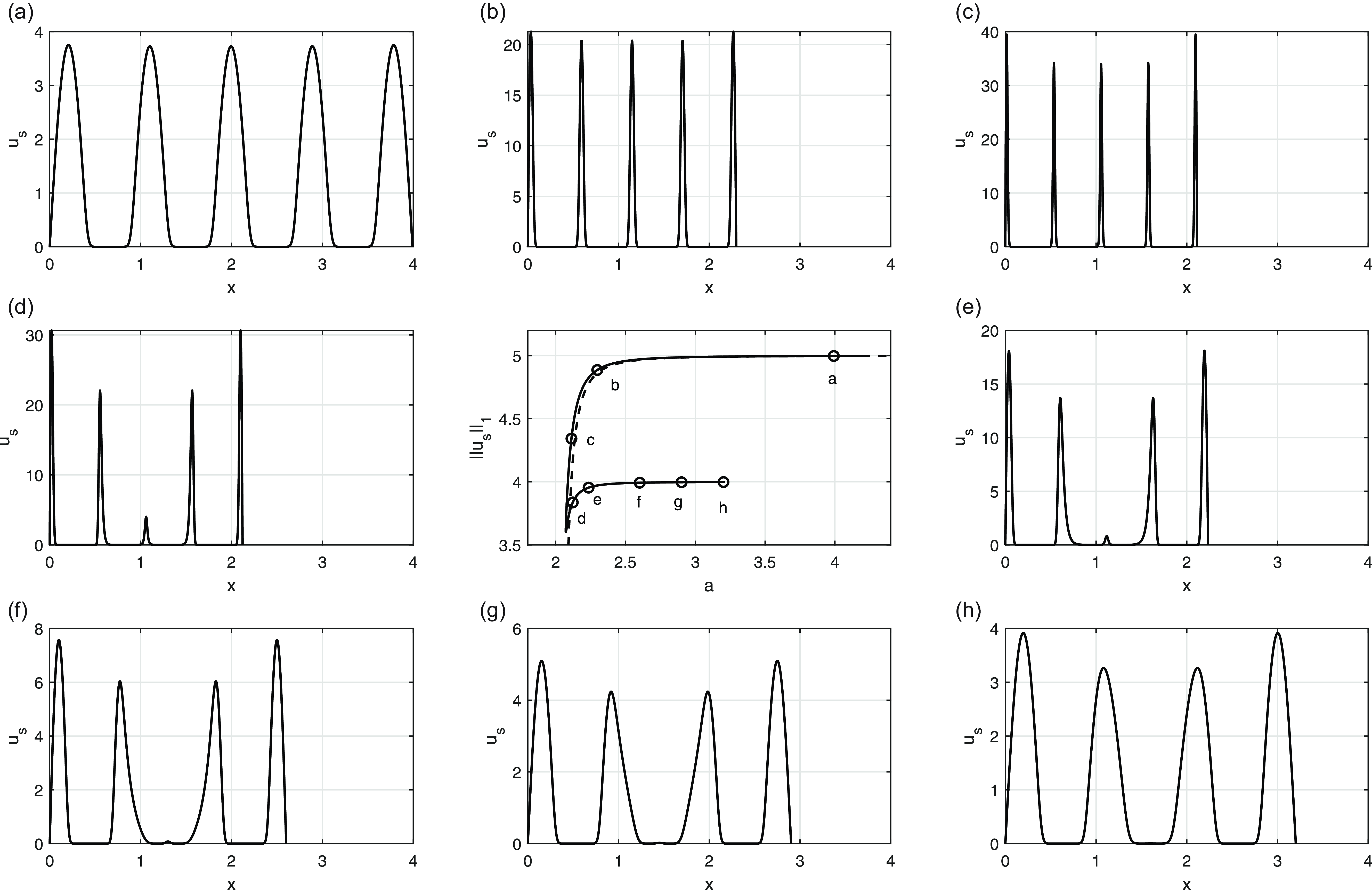
Figure 6. The profile of the steady state $u_s$
as the
$u_s$
as the $r=5$
to
$r=5$
to $r=4$
echelon of the bifurcation diagram is traversed. The central panel shows the relevant portion of the bifurcation diagram, with the broken line given by (80). The steady state in (a) of this figure is close to the steady state in (h) of the previous Figure 6 (see Figure 5, bottom right-hand panel) and is qualitatively very similar. Note the different
$r=4$
echelon of the bifurcation diagram is traversed. The central panel shows the relevant portion of the bifurcation diagram, with the broken line given by (80). The steady state in (a) of this figure is close to the steady state in (h) of the previous Figure 6 (see Figure 5, bottom right-hand panel) and is qualitatively very similar. Note the different $u_s$
-axis limits in the other panels, individually labelled (a) to (h), and identified on the central panel. Note that only solutions (a) to (c) are stable.
$u_s$
-axis limits in the other panels, individually labelled (a) to (h), and identified on the central panel. Note that only solutions (a) to (c) are stable.
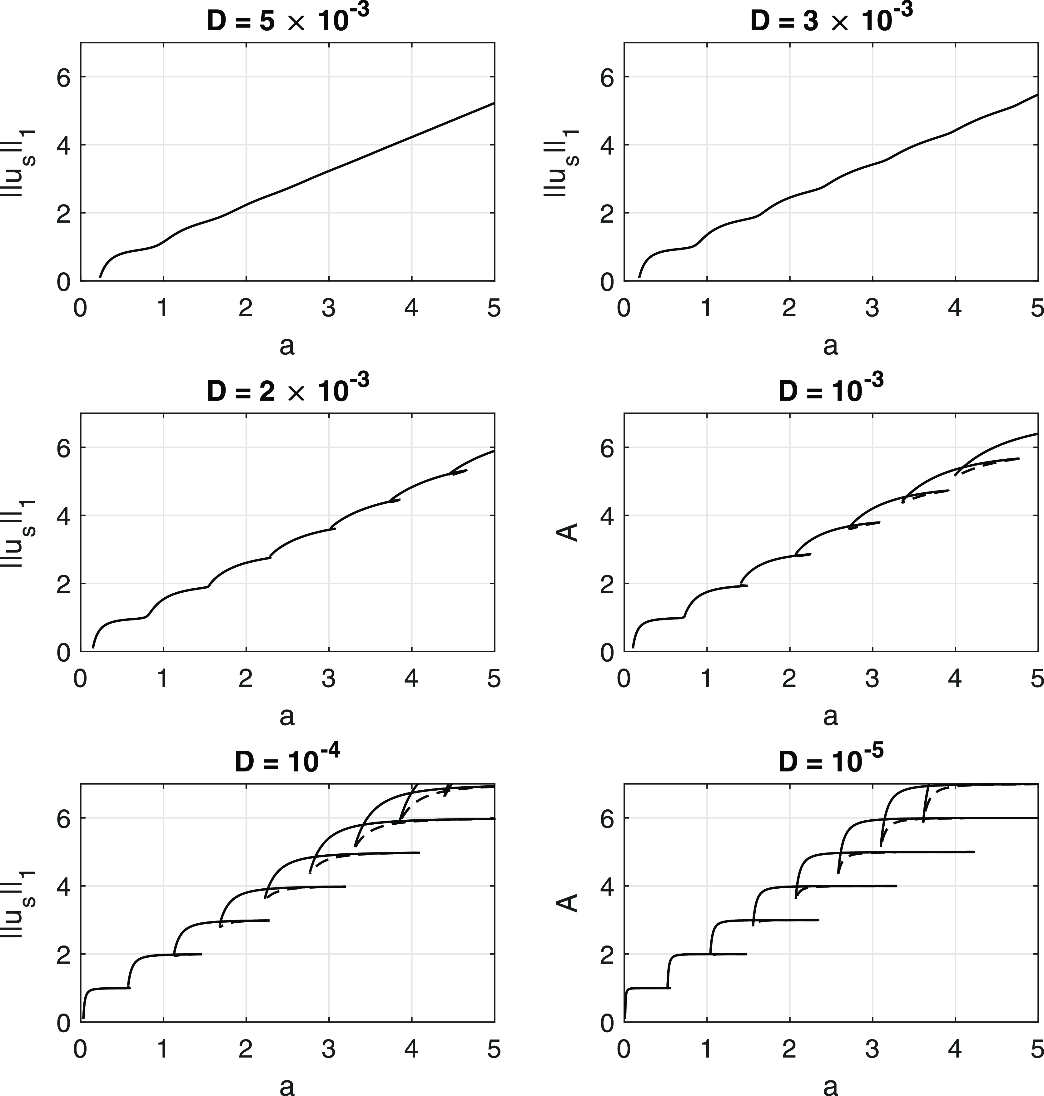
Figure 7. The $(a,||u_s||_1)$
bifurcation diagram for various values of
$(a,||u_s||_1)$
bifurcation diagram for various values of $D$
. Unstable branches are shown as broken lines.
$D$
. Unstable branches are shown as broken lines.
The steady state is uniformly approximated by (78), except in passive, thin, boundary layers at each end of the domain, when $x=O(D^{\frac {1}{2}})^+$
or
$x=O(D^{\frac {1}{2}})^+$
or $x=a-O(D^{\frac {1}{2}})^+$
, respectively, and in which
$x=a-O(D^{\frac {1}{2}})^+$
, respectively, and in which $u_s=O(D^{\frac {1}{2}})$
. In the
$u_s=O(D^{\frac {1}{2}})$
. In the $(a,||u_s(\cdot ,D,a)||_1)$
bifurcation plane, each branch of
$(a,||u_s(\cdot ,D,a)||_1)$
bifurcation plane, each branch of $r$
-peak steady states lies on the curve,
$r$
-peak steady states lies on the curve,
 \begin{equation} ||u_s(\cdot ,D,a)||_1 = r\left (1 - \frac {\pi ^2}{\left (\lambda (a,r)-\frac {1}{2}\right )^2}D + o(D^{\frac {5}{4}})\right )\,\,\text{as}\,\,D\to 0 \end{equation}
for $a \in (\frac {1}{2}(r-1) + O(D^{\frac {1}{2}})^+,r-\frac {1}{2}-O(D)^+)$
, as illustrated in the central panels of Figures 5 and 6, where this asymptotic expression can be seen to be in excellent agreement with the numerically calculated bifurcation curve. These overlapping branches form an increasing echelon as
$a \in (\frac {1}{2}(r-1) + O(D^{\frac {1}{2}})^+,r-\frac {1}{2}-O(D)^+)$
, as illustrated in the central panels of Figures 5 and 6, where this asymptotic expression can be seen to be in excellent agreement with the numerically calculated bifurcation curve. These overlapping branches form an increasing echelon as $r$
is successively increased, and each successive echelon is raised by unity, at leading order as
$r$
is successively increased, and each successive echelon is raised by unity, at leading order as $D\to 0$
. Each pair of overlapping echelon branches is connected by a loop, which consists of a very stiff subcritical saddle-node bifurcation at the head of each echelon, after which it then traces the echelon backwards, finally increasing towards the tail of the echelon, passing through a less stiff supercritical saddle-node bifurcation and then increasing by approximately unity to connect with the next echelon. Whilst traversing the loop, from head to tail, the additional peak is generated by either the minimum or maximum point at
$D\to 0$
. Each pair of overlapping echelon branches is connected by a loop, which consists of a very stiff subcritical saddle-node bifurcation at the head of each echelon, after which it then traces the echelon backwards, finally increasing towards the tail of the echelon, passing through a less stiff supercritical saddle-node bifurcation and then increasing by approximately unity to connect with the next echelon. Whilst traversing the loop, from head to tail, the additional peak is generated by either the minimum or maximum point at $x=\frac {1}{2}a$
pulling through itself, when
$x=\frac {1}{2}a$
pulling through itself, when $r$
is even or odd, respectively. This structure has been verified using pseudo-arclength continuation, and a typical numerically determined bifurcation diagram, for
$r$
is even or odd, respectively. This structure has been verified using pseudo-arclength continuation, and a typical numerically determined bifurcation diagram, for $D=10^{-5}$
, is shown in the final window of Figure 7. In addition, for the echelon-loop structure consisting of the
$D=10^{-5}$
, is shown in the final window of Figure 7. In addition, for the echelon-loop structure consisting of the $r=5$
and
$r=5$
and $r=6$
echelons, and then the
$r=6$
echelons, and then the $r=4$
and
$r=4$
and $r=5$
echelons, together with their corresponding loop connections, we graph, in Figure 5 and in Figure 6, a sequence of the associated steady states as the echelon-loop-echelon structure is traversed. In both figures, we give profiles from the upper echelon, moving backwards along this echelon onto the loop and through the lower supercritical saddle-node bifurcation, when the steady state begins its transition from a
$r=5$
echelons, together with their corresponding loop connections, we graph, in Figure 5 and in Figure 6, a sequence of the associated steady states as the echelon-loop-echelon structure is traversed. In both figures, we give profiles from the upper echelon, moving backwards along this echelon onto the loop and through the lower supercritical saddle-node bifurcation, when the steady state begins its transition from a $(r+1)$
-peak to an
$(r+1)$
-peak to an $r$
-peak form and then continue forwards along the loop towards the upper subcritical saddle-node bifurcation. We observe that the steady state profile is close to achieving its final
$r$
-peak form and then continue forwards along the loop towards the upper subcritical saddle-node bifurcation. We observe that the steady state profile is close to achieving its final $r$
-peak form prior to going through this upper saddle-node point, and so, for brevity, we stop giving profiles in both figures towards the upper end of the lower loop. We note the excellent agreement with the theory we have developed and presented above for
$r$
-peak form prior to going through this upper saddle-node point, and so, for brevity, we stop giving profiles in both figures towards the upper end of the lower loop. We note the excellent agreement with the theory we have developed and presented above for $D$
small. We also note, from (80) above, that the supercritical saddle-node bifurcation must take place in a region with
$D$
small. We also note, from (80) above, that the supercritical saddle-node bifurcation must take place in a region with $(a,||u_s||_1) = \left (\frac {1}{2}(r-1) -O(\sqrt {D}), r - O(1)\right )$
, whilst the subcritical saddle-node bifurcation should take place in a tighter region with
$(a,||u_s||_1) = \left (\frac {1}{2}(r-1) -O(\sqrt {D}), r - O(1)\right )$
, whilst the subcritical saddle-node bifurcation should take place in a tighter region with $(a,||u_s||_1) = \left (r-\frac {1}{2} + O(D), r - O(\sqrt {D}) \right )$
, as
$(a,||u_s||_1) = \left (r-\frac {1}{2} + O(D), r - O(\sqrt {D}) \right )$
, as $D\to 0$
. This is confirmed by the numerical results, as can be seen in the final panel of Figure 7. This completes the asymptotic structure for steady states when
$D\to 0$
. This is confirmed by the numerical results, as can be seen in the final panel of Figure 7. This completes the asymptotic structure for steady states when $D$
is small and
$D$
is small and $a\gt \frac {1}{2} + o(1).$
We now move on to the final case, with $D=O(1)$
and
$D=O(1)$
and $a\gt \pi \sqrt {D}$
.
$a\gt \pi \sqrt {D}$
.
2.2.6.
$D=O(1)$
with
$a\gt \pi \sqrt {D}$


In this final case, we first investigate numerically, using pseudo-arclength continuation. This provides strong evidence and support for us to formulate and propose the following key observations about the bifurcation structure in the $(a,||u_s||_1)$
bifurcation plane, for nontrivial, non-negative, steady states when
$(a,||u_s||_1)$
bifurcation plane, for nontrivial, non-negative, steady states when $D=O(1)$
and
$D=O(1)$
and $a\gt \pi \sqrt {D}$
:
$a\gt \pi \sqrt {D}$
:
-
• For each
$D\ge \Delta _1\approx 0.00297$
, the branch of single peak steady states created at the transcritical bifurcation from unity, when
$a=\pi \sqrt {D}$
, continues as a monotone increasing curve for all increasing
$a$
, with the associated steady state retaining a single peak structure for
$D\ge \Delta _m$
, but developing boundary oscillations about unity, which decay exponentially into the core for
$\Delta _1\le D \lt \Delta _m$
. In each case,
$||u_s||_1\sim a$
as
$a\to \infty$
, in agreement with section 2.2.4 above. There are no other non-negative steady state branches. The upper panels in Figure 7 show typical bifurcation curves. -
• For each
$0\lt D \lt \Delta _1$
, as
$a$
increases in the
$(a,||u_s||_1)$
bifurcation plane, first there is the single peak steady state, which emerges from the transcritical bifurcation from unity, when
$a=\pi \sqrt {D}$
. Thereafter, for each
$r=2,3,4,\ldots$
, there is an interval
$K_r(D)=[a_r(D),b_r(D)]$
, with
$\{a_r(D)\},\,\{b_r(D)\}$
both being positive, strictly increasing and unbounded sequences in
$r=2,3,\ldots$
, such that for each
$a\in K_r(D)$
, there is an
$r$
-peak nontrivial and non-negative steady state, and this has
$||u_s||_1 = O(r)$
on
$K_r(D)$
. It follows from the theory above in section 2.2.4, for
$a$
large with
$D=O(1)$
, that
$a_r(D)\sim \lambda _1^-(D)r$
and
$b_r(D)\sim \lambda _1^+(D)r$
as
$r\to \infty$
. In addition, there is a natural number
$r_c(D) = \lfloor \lambda _1^-(D)/(\lambda _1^+(D)-\lambda _1^-(D)) \rfloor +1 \ge 2$
, which is decreasing as
$D$
decreases, with
$r_c(0^+) = 2$
and
$r_c(D)\to \infty$
as
$D \to \Delta _1^-$
, and for which
$a_{r+1}(D)\gt b_r(D)$
when
$2\le r \lt r_c(D)$
whilst
$a_{r+1}(D)\le b_r(D)$
for
$r\ge r_c(D)$
. When
$2\le r\lt r_c(D)$
, the connection between the
$r^{th}$
and
$(r+1)^{th}$
echeloned branch is a monotone increasing curve in the
$(a,||u_s||_1)$
bifurcation diagram, with the associated steady state smoothly transitioning from an
$r$
-peak to an
$(r+1)$
-peak steady state. However, for
$r\ge r_c(D)$
, the lower end of the
$(r+1)^{th}$
echelon now overlaps the upper end of the
$r^{th}$
echelon, and the connection is now via a loop, which has the qualitative character of the loops visible in the numerical examples illustrated in Figure 7. As a particular illustration of this case, Figure 3 shows the
$(a,||u_s||_1)$
bifurcation diagram for
$D=2\times 10^{-3}$
, obtained numerically using pseudo-arclength continuation. For the same case, Figure 4 examines in detail the
$r=14$
echelon, with the transitional loop connecting to the
$r=13$
echelon. Associated steady state profiles are presented at points along the upper echelon and on the loop.


Each situation has now been considered. A point of interest to note is that the appearance of the multiple saddle-node loops in the $(a,||u_s||_1)$
bifurcation diagram, at each fixed
$(a,||u_s||_1)$
bifurcation diagram, at each fixed $D$
below
$D$
below $\Delta _1\approx 0.00297$
, will obviously generate multiple hysteresis behaviour in the evolution of stable steady states when the parameter
$\Delta _1\approx 0.00297$
, will obviously generate multiple hysteresis behaviour in the evolution of stable steady states when the parameter $a$
is slowly increased and then slowly decreased.
$a$
is slowly increased and then slowly decreased.
This completes the study of nontrivial, non-negative steady states for $a\gt 1/2$
. We are now in a position to return to the evolution problem (DIVP) at parameter values
$a\gt 1/2$
. We are now in a position to return to the evolution problem (DIVP) at parameter values $(a,D)$
with
$(a,D)$
with $a\gt 1/2$
and
$a\gt 1/2$
and $0\lt D\lt \pi ^2/a^2$
, which we label as region
$0\lt D\lt \pi ^2/a^2$
, which we label as region $\mathcal{H}$
. We begin by addressing the local stability properties of the nontrivial, non-negative steady states, identified and investigated in the above subsections, at each point
$\mathcal{H}$
. We begin by addressing the local stability properties of the nontrivial, non-negative steady states, identified and investigated in the above subsections, at each point $(a,D)\in \mathcal{H}$
, recalling from above that at each such point there is either,
$(a,D)\in \mathcal{H}$
, recalling from above that at each such point there is either,
-
• a single
$r$
-peak, nontrivial, non-negative steady state, for some
$r\in \mathbb{N}$
, when we label
$(a,D)\in \mathcal{H}_1$
, or, -
• an odd number, larger than unity, of nontrivial, non-negative steady states, these being an
$r$
-peak, an
$(r+1)$
-peak and a transitional steady state, from a minimum value of
$r(\ge 2)$
to a maximum value of
$r$
(which becomes unbounded with increasing
$a$
at fixed
$D\lt \Delta _1$
) when we label
$(a,D)\in \mathcal{H}_2$
. For
$D$
small, the minimum and maximum values of
$r$
are well approximated by the integer parts of
$(a+\frac {1}{2})$
and
$(2a+1)$
, respectively, which is readily determined via the asymptotic analysis presented in subsection 2.2.5.


It is again helpful to fix $D$
and then follow the nontrivial and non-negative steady state bifurcation curve in the
$D$
and then follow the nontrivial and non-negative steady state bifurcation curve in the $(a,||u_s||_1)$
bifurcation plane. As this curve is followed from the initial transcritical bifurcation at
$(a,||u_s||_1)$
bifurcation plane. As this curve is followed from the initial transcritical bifurcation at $a=\pi \sqrt {D}$
to large
$a=\pi \sqrt {D}$
to large $a$
, computational results determine that the largest eigenvalue of the linear stability problem (see Appendix B), which is zero at the small norm transcritical bifurcation, becomes negative with increasing
$a$
, computational results determine that the largest eigenvalue of the linear stability problem (see Appendix B), which is zero at the small norm transcritical bifurcation, becomes negative with increasing $a$
, and remains negative unless a fold is traversed, in which case it changes sign to positive, returning to negative after the next fold is traversed, with this pattern continuing as the bifurcation curve is continuously traversed. This enables us to conclude that at any point
$a$
, and remains negative unless a fold is traversed, in which case it changes sign to positive, returning to negative after the next fold is traversed, with this pattern continuing as the bifurcation curve is continuously traversed. This enables us to conclude that at any point $(a,D)\in \mathcal{H}_1$
, then the
$(a,D)\in \mathcal{H}_1$
, then the $r$
-peak steady state is linearly stable, whilst when
$r$
-peak steady state is linearly stable, whilst when $(a,D)\in \mathcal{H}_3$
, for each
$(a,D)\in \mathcal{H}_3$
, for each $r$
, both the
$r$
, both the $r$
-peak and the
$r$
-peak and the $(r+1)$
-peak steady states are linearly stable, with the transitional steady state being linearly unstable. Figures 8 and 9 show the dependence on
$(r+1)$
-peak steady states are linearly stable, with the transitional steady state being linearly unstable. Figures 8 and 9 show the dependence on $a$
of the value of the largest eigenvalue at each point on the bifurcation curve, at two representative values of
$a$
of the value of the largest eigenvalue at each point on the bifurcation curve, at two representative values of $D$
, namely
$D$
, namely $D=10^{-5}$
and
$D=10^{-5}$
and $D=2\times 10^{-3}$
, respectively. The eigenvalues are determined by pseudo-arclength continuation following the steady state bifurcation curve, and formulating and numerically solving the associated linear eigenvalue problem. The points which have zero largest eigenvalue correspond to the upper and lower saddle-node bifurcations on each echelon-loop-echelon cycle, with the largest eigenvalue being negative on the echelons, and positive on the loops.
$D=2\times 10^{-3}$
, respectively. The eigenvalues are determined by pseudo-arclength continuation following the steady state bifurcation curve, and formulating and numerically solving the associated linear eigenvalue problem. The points which have zero largest eigenvalue correspond to the upper and lower saddle-node bifurcations on each echelon-loop-echelon cycle, with the largest eigenvalue being negative on the echelons, and positive on the loops.
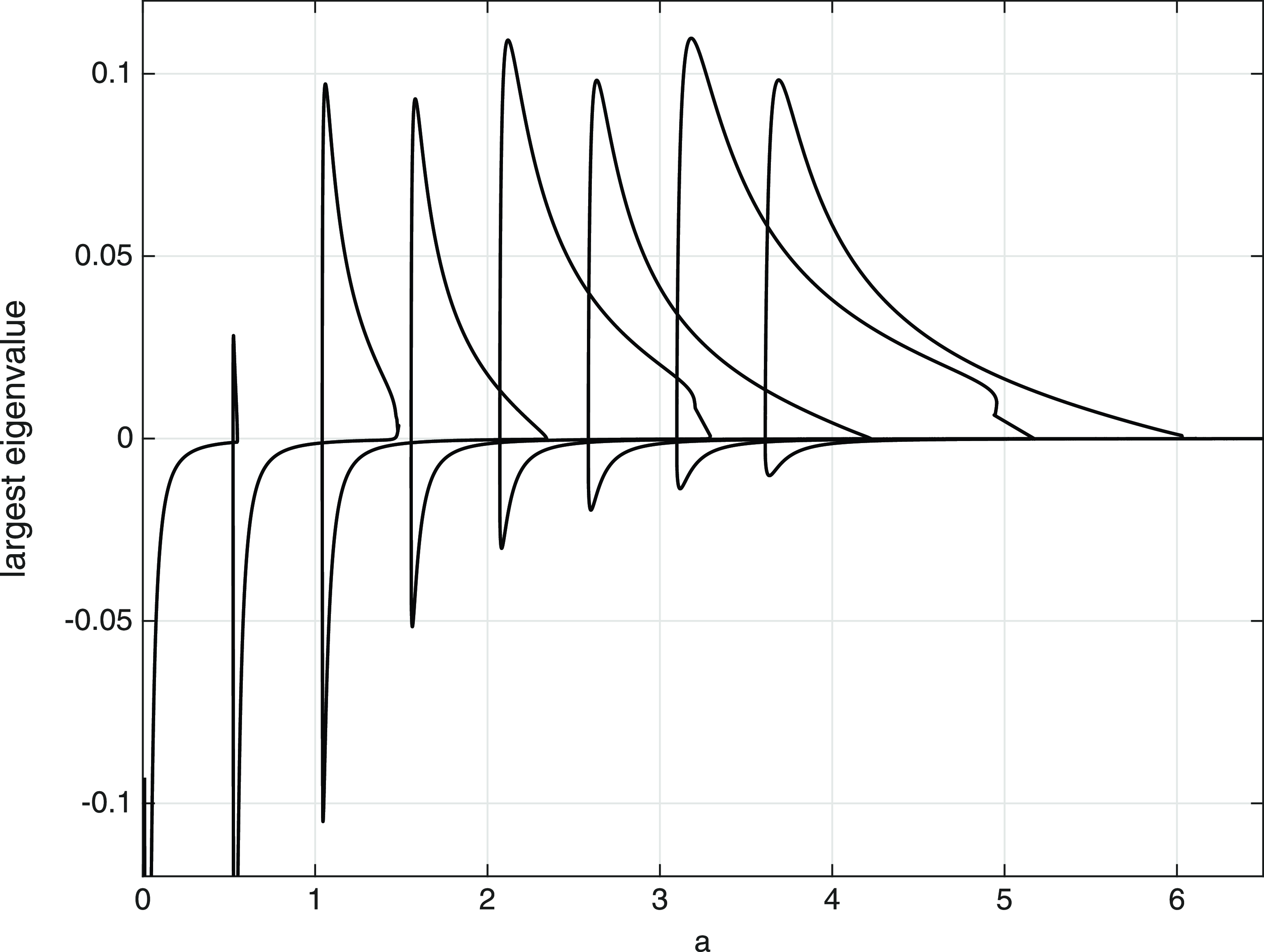
Figure 8. The dependence on $a$
of the largest eigenvalue of the linear stability problem for
$a$
of the largest eigenvalue of the linear stability problem for $D = 10^{-5}$
as the bifurcation curve is traversed. Note the slight qualitative difference in the plot between steady states with odd and even numbers of peaks.
$D = 10^{-5}$
as the bifurcation curve is traversed. Note the slight qualitative difference in the plot between steady states with odd and even numbers of peaks.
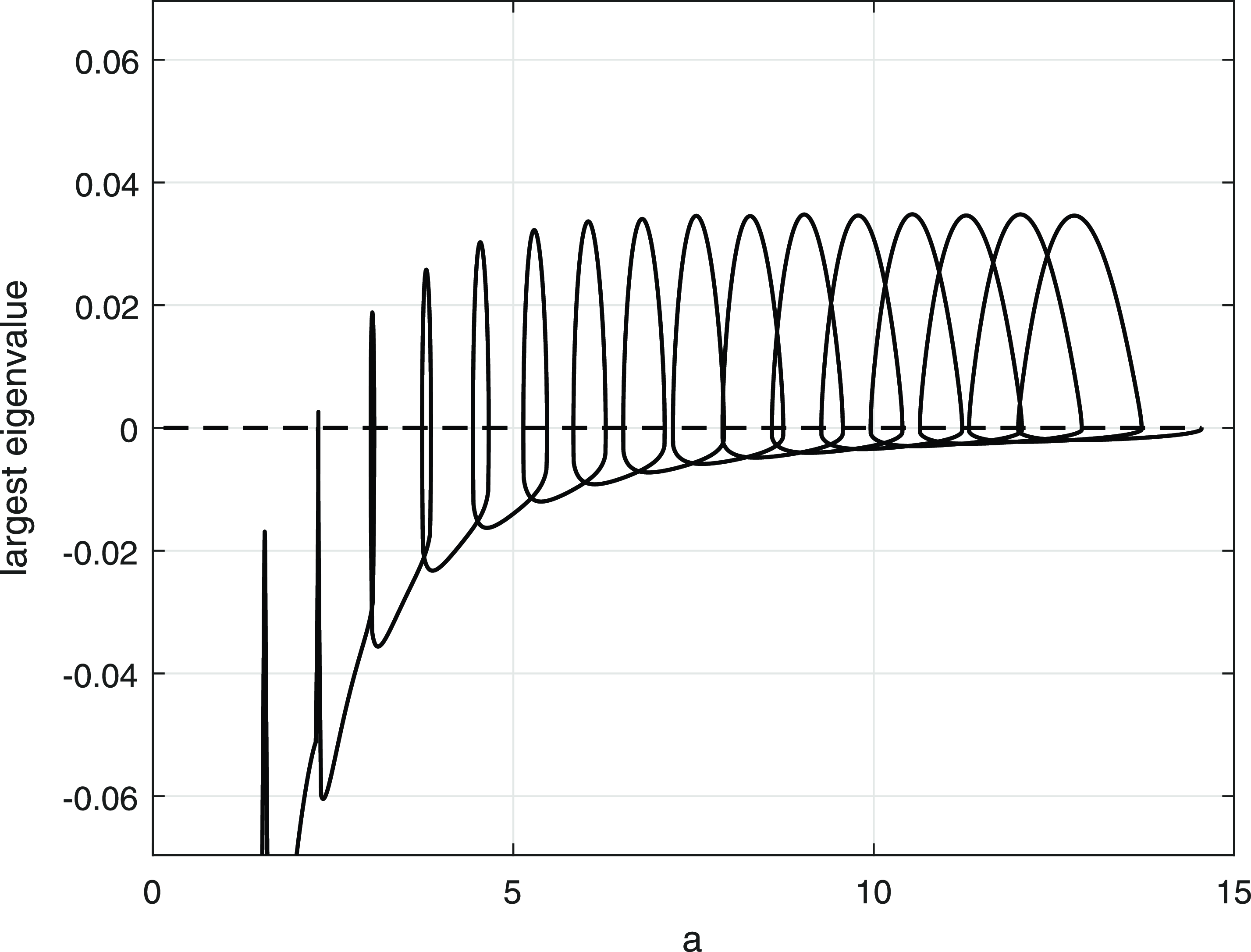
Figure 9. The dependence on $a$
of the largest eigenvalue of the linear stability problem for
$a$
of the largest eigenvalue of the linear stability problem for $D = 2 \times 10^{-3}$
as the bifurcation curve is traversed.
$D = 2 \times 10^{-3}$
as the bifurcation curve is traversed.
Interpreting this in relation to (DIVP), we conjecture that :
-
• For
$(a,D)\in \mathcal{H}_1$
, the solution to (DIVP) approaches the stable and unique
$r$
-peak steady state as
$t\to \infty$
uniformly for
$x\in [0,a]$
. -
• For
$(a,D)\in \mathcal{H}_2$
, the solution to (DIVP) approaches one of either the stable
$r$
-peak or the stable
$(r+1)$
-peak steady state, for some
$r$
between the available minimum and maximum, depending upon the initial data
$u_0\;:\;[0,a]\to \mathbb{R}$
, as
$t\to \infty$
uniformly for
$x\in [0,a]$
.


To support this conjecture, we have solved (DIVP) numerically (see Appendix A for details) for initial conditions of the form
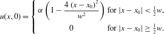 \begin{equation} u(x,0) = \left \{ \begin{array}{cc} \alpha \left (1-\dfrac {4\left (x-x_0\right )^2}{w^2}\right ) & \mbox{for $|x-x_0|\lt \frac {1}{2}w$},\\[10pt] 0 & \mbox{for $|x-x_0| \geq \frac {1}{2}w$.} \end{array}\right . \end{equation}
This is a localised initial input of $u$
based at
$u$
based at $x_0$
, with width
$x_0$
, with width $w$
and height
$w$
and height $\alpha$
, each chosen so that the support of
$\alpha$
, each chosen so that the support of $u(x,0)$
is contained in
$u(x,0)$
is contained in $[0,a]$
. This type of localised initial condition is representative of the type of initial distribution arising in applications. For
$[0,a]$
. This type of localised initial condition is representative of the type of initial distribution arising in applications. For $D=2\times 10^{-3}$
and
$D=2\times 10^{-3}$
and $a=10$
, two numerical solutions, with small, localised inputs of
$a=10$
, two numerical solutions, with small, localised inputs of $u$
(
$u$
( $\alpha = 0.01$
,
$\alpha = 0.01$
, $w = 0.1$
) are shown in Figure 10. In each case, initially, a pair of wavefronts is generated, which propagate away from
$w = 0.1$
) are shown in Figure 10. In each case, initially, a pair of wavefronts is generated, which propagate away from $x = x_0$
. In the symmetric case (top row),
$x = x_0$
. In the symmetric case (top row), $x_0 = 5$
, these reach the boundaries simultaneously and a steady state with
$x_0 = 5$
, these reach the boundaries simultaneously and a steady state with $13$
peaks is generated. In the bottom row,
$13$
peaks is generated. In the bottom row, $x_0 = 2.5$
, and the wavefronts reach the boundaries at different times. In this case, a steady state with
$x_0 = 2.5$
, and the wavefronts reach the boundaries at different times. In this case, a steady state with $14$
peaks is generated. Figure 3 shows that when
$14$
peaks is generated. Figure 3 shows that when $a=10$
, there are actually three temporally stable steady states available, with
$a=10$
, there are actually three temporally stable steady states available, with $r = 13$
,
$r = 13$
, $14$
and
$14$
and $15$
. Whatever value we choose for
$15$
. Whatever value we choose for $x_0$
, numerical solutions indicate that the
$x_0$
, numerical solutions indicate that the $r=15$
steady state is not generated using these initial conditions, and we hypothesise that this is because the slightly shorter wavelength of the
$r=15$
steady state is not generated using these initial conditions, and we hypothesise that this is because the slightly shorter wavelength of the $r=15$
steady state is too far from the natural wavelength generated behind the wavefronts when the Cauchy problem is on the whole real line, as determined in (NB1).
$r=15$
steady state is too far from the natural wavelength generated behind the wavefronts when the Cauchy problem is on the whole real line, as determined in (NB1).
The analysis of the Dirichlet problem (DIVP) is now complete, and we move on to consider the Neumann problem (NIVP).
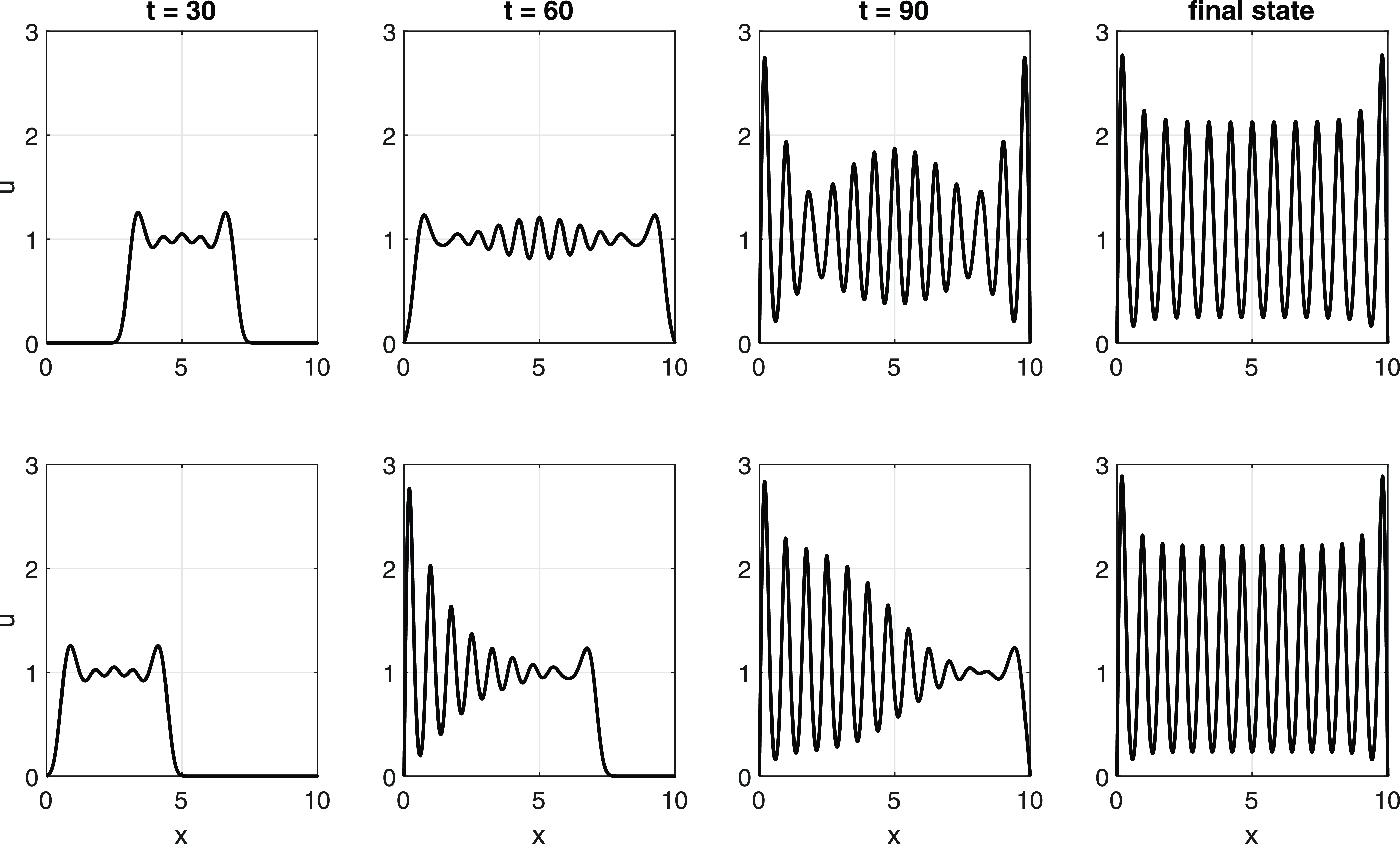
Figure 10. Solutions of (DIVP) for two different initial conditions, with $a=10$
and
$a=10$
and $D = 2 \times 10^{-3}$
. In the top row, the initial small input of
$D = 2 \times 10^{-3}$
. In the top row, the initial small input of $u$
lies symmetrically at
$u$
lies symmetrically at $x_0 = 5$
and generates a steady state with 13 peaks. In the bottom row, the initial small input of
$x_0 = 5$
and generates a steady state with 13 peaks. In the bottom row, the initial small input of $u$
lies at
$u$
lies at $x_0 = 2.5$
and generates a steady state with 14 peaks. In each case,
$x_0 = 2.5$
and generates a steady state with 14 peaks. In each case, $w = 0.1$
and
$w = 0.1$
and $\alpha = 0.01$
.
$\alpha = 0.01$
.
3. The Neumann problem (NIVP)
In this section, we analyse the Neumann problem (NIVP). The analysis is very similar to that in section 2 for the Dirichlet problem (DIVP), and so we focus mainly on presenting the key results, avoiding repetition where possible. When the initial data are trivial, the solution to the associated (NIVP) is again the equilibrium solution given in (12). For initial data with $||u_0||_{\infty }$
small, it is again straightforward to develop a linearised theory for (NIVP), and this readily determines that the trivial equilibrium solution is unstable for all
$||u_0||_{\infty }$
small, it is again straightforward to develop a linearised theory for (NIVP), and this readily determines that the trivial equilibrium solution is unstable for all $(a,D)\in (0,\infty )\times (0,\infty )$
.
$(a,D)\in (0,\infty )\times (0,\infty )$
.
Again, we recall from the introduction that in the limit $D\to \infty$
(after rescaling
$D\to \infty$
(after rescaling $x$
with
$x$
with $\sqrt {D}$
), (NIVP) becomes the classical local Fisher-KPP Neumann problem, and so the associated well known classical results for this local problem are recovered in this limit, and this is confirmed in what follows below.
$\sqrt {D}$
), (NIVP) becomes the classical local Fisher-KPP Neumann problem, and so the associated well known classical results for this local problem are recovered in this limit, and this is confirmed in what follows below.
3.1.
$0\lt a\le 1/2$

We first consider (NIVP) when $0\lt a\le 1/2$
, and so equation (1) takes on the form of (13) with (14). To begin, it is a simple direct calculation to show that the only nontrivial steady state that exists is the constant steady state,
$0\lt a\le 1/2$
, and so equation (1) takes on the form of (13) with (14). To begin, it is a simple direct calculation to show that the only nontrivial steady state that exists is the constant steady state,
 \begin{equation} u_s(x,D,a) = a^{-1}\,\,\forall \,\,(x,t)\in \bar {D}_{\infty }. \end{equation}
Moreover, the solution to (NIVP) can be determined exactly, and is given by,
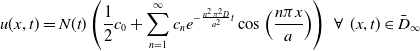 \begin{equation} u(x,t) = N(t)\left (\frac {1}{2}c_0 + \sum _{n=1}^{\infty }c_n e^{-\frac {n^2\pi ^2D}{a^2}t}\cos \left (\frac {n\pi x}{a}\right )\right )\,\,\forall \,\,(x,t)\in \bar {D}_{\infty } \end{equation}
with
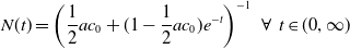 \begin{equation} N(t) = \left ( \frac {1}{2}ac_0 + (1-\frac {1}{2}ac_0)e^{-t}\right )^{-1}\,\,\forall \,\,t\in (0,\infty ) \end{equation}
and
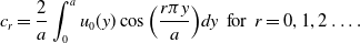 \begin{equation} c_r = \frac {2}{a}\int _0^a{u_0(y)\cos \left (\frac {r\pi y}{a}\right )}dy\,\,\text{for}\,\,r=0,1,2\ldots . \end{equation}
We observe that for all nontrivial initial data,
 \begin{equation} u(x,t) \to a^{-1}\,\,\text{as}\,\,t\to \infty , \end{equation}
uniformly for $x\in [0,a]$
. This establishes that the constant steady state
$x\in [0,a]$
. This establishes that the constant steady state $a^{-1}$
is globally asymptotically stable. This case is now complete.
$a^{-1}$
is globally asymptotically stable. This case is now complete.
3.2.
$a\gt 1/2$

Here we consider (NIVP) when $a\gt 1/2$
. As before, we begin by considering the possible nontrivial and non-negative steady states of equation (1). Again, it is convenient to fix
$a\gt 1/2$
. As before, we begin by considering the possible nontrivial and non-negative steady states of equation (1). Again, it is convenient to fix $D\gt 0$
and increase
$D\gt 0$
and increase $a\gt 1/2$
, starting by continuing from the unique constant steady state
$a\gt 1/2$
, starting by continuing from the unique constant steady state $u_s = 2$
, when
$u_s = 2$
, when $a=1/2$
. There are a number of cases where we can develop an asymptotic theory for steady states, and we deal with these first. We begin by considering this when
$a=1/2$
. There are a number of cases where we can develop an asymptotic theory for steady states, and we deal with these first. We begin by considering this when $D$
is large.
$D$
is large.
3.2.1.
$D\gg 1$

There are two cases. First, we address the case when $a\in (1/2,o(\sqrt {D}))$
as
$a\in (1/2,o(\sqrt {D}))$
as $D\to \infty$
, and expand any possible steady state in the regular perturbation form
$D\to \infty$
, and expand any possible steady state in the regular perturbation form
 \begin{equation} u_s(x,D,a) = \bar {u}_0(x,a) + D^{-1}\bar {u}_1(x,a) + O(D^{-2})\,\,\text{as}\,\,D\to \infty , \end{equation}
uniformly for $x\in [0,a]$
. After substitution into equation (1) and boundary conditions (8), and solving the resulting problem directly, we find that
$x\in [0,a]$
. After substitution into equation (1) and boundary conditions (8), and solving the resulting problem directly, we find that
 \begin{equation} \bar {u}_0(x,a) = c(a)\,\,\forall \,\,x\in [0,a], \end{equation}
with $c(a)$
a positive constant to be determined. At next order, we obtain the following linear, inhomogeneous boundary value problem for
$c(a)$
a positive constant to be determined. At next order, we obtain the following linear, inhomogeneous boundary value problem for $\bar {u}_1$
, namely,
$\bar {u}_1$
, namely,
 \begin{equation} \bar {u}''_{1} = c(a)\left (1 - c(a)\phi (x,a)\right ),\,\,x\in (0,a), \end{equation}
 \begin{equation} \bar {u}'_{1}(0,a)=\bar {u}'_1(a,a)=0. \end{equation}
Here, for $1/2\lt a\lt 1$
,
$1/2\lt a\lt 1$
,
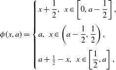 \begin{equation} \phi (x,a)= \begin{cases} x+\dfrac {1}{2},\,\,x\in \left[0,a-\dfrac {1}{2}\right],\\[12pt] a,\,\,x\in \left(a-\dfrac {1}{2},\dfrac {1}{2}\right), \\[12pt] a+\frac {1}{2}-x,\,\,x\in \left[\dfrac {1}{2}, a\right], \end{cases} \end{equation}
whilst for $a\ge 1$
,
$a\ge 1$
,
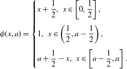 \begin{equation} \phi (x,a)= \begin{cases} x+\dfrac {1}{2},\,\,x\in \left[0,\dfrac {1}{2}\right],\\[12pt] 1,\,\,x\in \left(\dfrac {1}{2},a-\dfrac {1}{2}\right), \\[12pt] a+\dfrac {1}{2}-x,\,\,x\in \left[a-\dfrac {1}{2}, a\right]. \end{cases} \end{equation}
The solution to this linear boundary value problem is obtained directly and has,
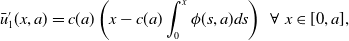 \begin{equation} \bar {u}'_1(x,a) = c(a)\left (x - c(a)\int _0^x{\phi (s,a)}ds\right )\,\,\forall \,\,x\in [0,a], \end{equation}
with now $c(a)$
being required to satisfy the solvability condition,
$c(a)$
being required to satisfy the solvability condition,
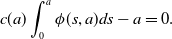 \begin{equation} c(a)\int _0^a{\phi (s,a)}ds - a = 0. \end{equation}
Equation (94) has the unique positive solution,
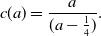 \begin{equation} c(a) = \frac {a}{(a-\frac {1}{4})}. \end{equation}
Thus, for each $a\in (1/2,o(\sqrt {D}))$
, there is a unique, nontrivial and non-negative steady state, which has,
$a\in (1/2,o(\sqrt {D}))$
, there is a unique, nontrivial and non-negative steady state, which has,
 \begin{equation} u_s(x,D,a) = \frac {a}{(a-\frac {1}{4})}\, +\,D^{-1}\left (c(a)\int _0^x{\left (y - c(a)\int _0^y{\phi (s,a)}ds\right )}dy + d(a)\right )\, +\,O(D^{-2}), \end{equation}
as $D\to \infty$
, uniformly for
$D\to \infty$
, uniformly for $x\in [0,a]$
, with the constant
$x\in [0,a]$
, with the constant $d(a)$
determined via a solvability condition at
$d(a)$
determined via a solvability condition at $O(D^{-2})$
. It should be noted that this steady state is, as it should be, an even function about
$O(D^{-2})$
. It should be noted that this steady state is, as it should be, an even function about $x=\frac {1}{2}a$
. We now observe that expansion (96) becomes nonuniform when
$x=\frac {1}{2}a$
. We now observe that expansion (96) becomes nonuniform when $a = O(\sqrt {D})$
as
$a = O(\sqrt {D})$
as $D\to \infty$
. Therefore, to continue this unique branch of steady states for
$D\to \infty$
. Therefore, to continue this unique branch of steady states for $a$
large, we first write,
$a$
large, we first write,
 \begin{equation} a = \sqrt {D} \bar {a}\,\,\text{and}\,\,x=\sqrt {D}\bar {x}, \end{equation}
with $\bar {a}=O(1)^+$
and
$\bar {a}=O(1)^+$
and $\bar {x}\in [0,\bar {a}]$
as
$\bar {x}\in [0,\bar {a}]$
as $D\to \infty$
. It then follows from (95) and (96) that we should expand possible steady states in the asymptotic form,
$D\to \infty$
. It then follows from (95) and (96) that we should expand possible steady states in the asymptotic form,
 \begin{equation} u_s(\bar {x},D,\bar {a}) = 1 + D^{-\frac {1}{2}}U_0(\bar {x},\bar {a}) + O(D^{-1})\,\,\text{as}\,\,D\to \infty , \end{equation}
for $\bar {x}\in [0,\bar {a}]$
. After substitution into equation (1) and boundary conditions (8), and solving the resulting problem directly, we find that at leading order, the only solution, which has the required symmetry about
$\bar {x}\in [0,\bar {a}]$
. After substitution into equation (1) and boundary conditions (8), and solving the resulting problem directly, we find that at leading order, the only solution, which has the required symmetry about $\bar {x}=\frac {1}{2}\bar {a}$
, is given by,
$\bar {x}=\frac {1}{2}\bar {a}$
, is given by,
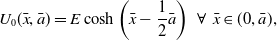 \begin{equation} U_0(\bar {x},\bar {a}) = E\cosh \left (\bar {x}-\frac {1}{2}\bar {a}\right )\,\,\forall \,\,\bar {x}\in (0,\bar {a}), \end{equation}
with $E$
a constant to be determined. We now observe that this leading order term fails to satisfy the Neumann boundary conditions at the interval end points, and we conclude that two symmetric boundary layers are required in the neighbourhood of each respective end point, and we adopt the method of matched asymptotic expansions. We will consider the boundary layer at the end
$E$
a constant to be determined. We now observe that this leading order term fails to satisfy the Neumann boundary conditions at the interval end points, and we conclude that two symmetric boundary layers are required in the neighbourhood of each respective end point, and we adopt the method of matched asymptotic expansions. We will consider the boundary layer at the end $\bar {x}=0$
. A balancing of terms determines that the boundary layer has
$\bar {x}=0$
. A balancing of terms determines that the boundary layer has $\bar {x} = O(D^{-\frac {1}{2}})$
, and so
$\bar {x} = O(D^{-\frac {1}{2}})$
, and so $x=O(1)$
, as
$x=O(1)$
, as $D\to \infty$
, and we are led to expand in the asymptotic form,
$D\to \infty$
, and we are led to expand in the asymptotic form,
 \begin{equation} u_s(x,D,\bar {a}) = 1 + D^{-\frac {1}{2}}{U}^0(x,\bar {a}) + D^{-1}{U}^1(x,\bar {a}) + O(D^{-\frac {3}{2}})\,\,\text{for}\,\,x\ge 0, \end{equation}
as $D\to \infty$
. On substitution into equation (1), solving at each order, and applying the boundary condition at
$D\to \infty$
. On substitution into equation (1), solving at each order, and applying the boundary condition at $x=0$
, we obtain,
$x=0$
, we obtain,
 \begin{equation} {U}^0(x,\bar {a}) = F, \end{equation}
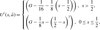 \begin{equation} {U}^1(x,\bar {a}) = \begin{cases} \left (G-\dfrac {1}{16}-\dfrac {1}{8}\left(x-\dfrac {1}{2}\right)\right ),\,\,x\gt \dfrac {1}{2},\\[12pt] \left (G - \dfrac {1}{8}x - \left(\dfrac {1}{2}-x\right)^3\right ),\,\,0\le x\le \dfrac {1}{2}, \end{cases} \end{equation}
with $F$
and
$F$
and $G$
constants to be determined via asymptotic matching to the core region. Matching (via Van Dyke’s Principle) expansion (98) (as
$G$
constants to be determined via asymptotic matching to the core region. Matching (via Van Dyke’s Principle) expansion (98) (as $\bar {x}\to 0$
) with expansion (100) (as
$\bar {x}\to 0$
) with expansion (100) (as $x\to \infty$
) determines,
$x\to \infty$
) determines,
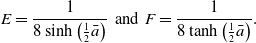 \begin{equation} E = \frac {1}{8\,\text{sinh}\left (\frac {1}{2}\bar {a}\right )}\,\,\text{and}\,\,F= \frac {1}{8\,\text{tanh}\left (\frac {1}{2}\bar {a}\right )}. \end{equation}
However, the determination of the constant $G$
requires the next term in the core region to be found, which, for brevity, we need not pursue further.
$G$
requires the next term in the core region to be found, which, for brevity, we need not pursue further.
We now make a comparison between the asymptotic forms for steady states, derived above from the full problem and valid for $D \gg 1$
, and the numerical solutions obtained by pseudo-arclength continuation following steady states of the full problem. This is done most conveniently by plotting the value of the steady state at the midpoint of the domain (minus one for clarity in a semi-logarithmic plot),
$D \gg 1$
, and the numerical solutions obtained by pseudo-arclength continuation following steady states of the full problem. This is done most conveniently by plotting the value of the steady state at the midpoint of the domain (minus one for clarity in a semi-logarithmic plot), $u_s\left (\frac {1}{2}a\right ) -1$
, as a function of
$u_s\left (\frac {1}{2}a\right ) -1$
, as a function of $a\gt \frac {1}{2}$
for various values of
$a\gt \frac {1}{2}$
for various values of $D$
, and compare with the leading order Van Dyke composite asymptotic form (see [Reference Van Dyke18]) for
$D$
, and compare with the leading order Van Dyke composite asymptotic form (see [Reference Van Dyke18]) for $u_s\left (\frac {1}{2}a\right )$
, given by
$u_s\left (\frac {1}{2}a\right )$
, given by
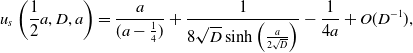 \begin{equation} u_s\left (\frac {1}{2}a,D,a\right ) = \frac {a}{(a-\frac {1}{4})}+\frac {1}{8 \sqrt {D} \sinh \left (\frac {a}{2\sqrt {D}}\right )}-\frac {1}{4a} + O(D^{-1}), \end{equation}
as $D\to 0$
, and obtained from the matched asymptotic expansions (96) and (98) above. This gives the leading order approximation uniformly for all
$D\to 0$
, and obtained from the matched asymptotic expansions (96) and (98) above. This gives the leading order approximation uniformly for all $a\gt \frac {1}{2}$
when
$a\gt \frac {1}{2}$
when $D \gg 1$
. Figure 11 shows how the agreement between the numerically determined steady state and leading order composite asymptotic form of the steady state improves as
$D \gg 1$
. Figure 11 shows how the agreement between the numerically determined steady state and leading order composite asymptotic form of the steady state improves as $D$
increases.
$D$
increases.
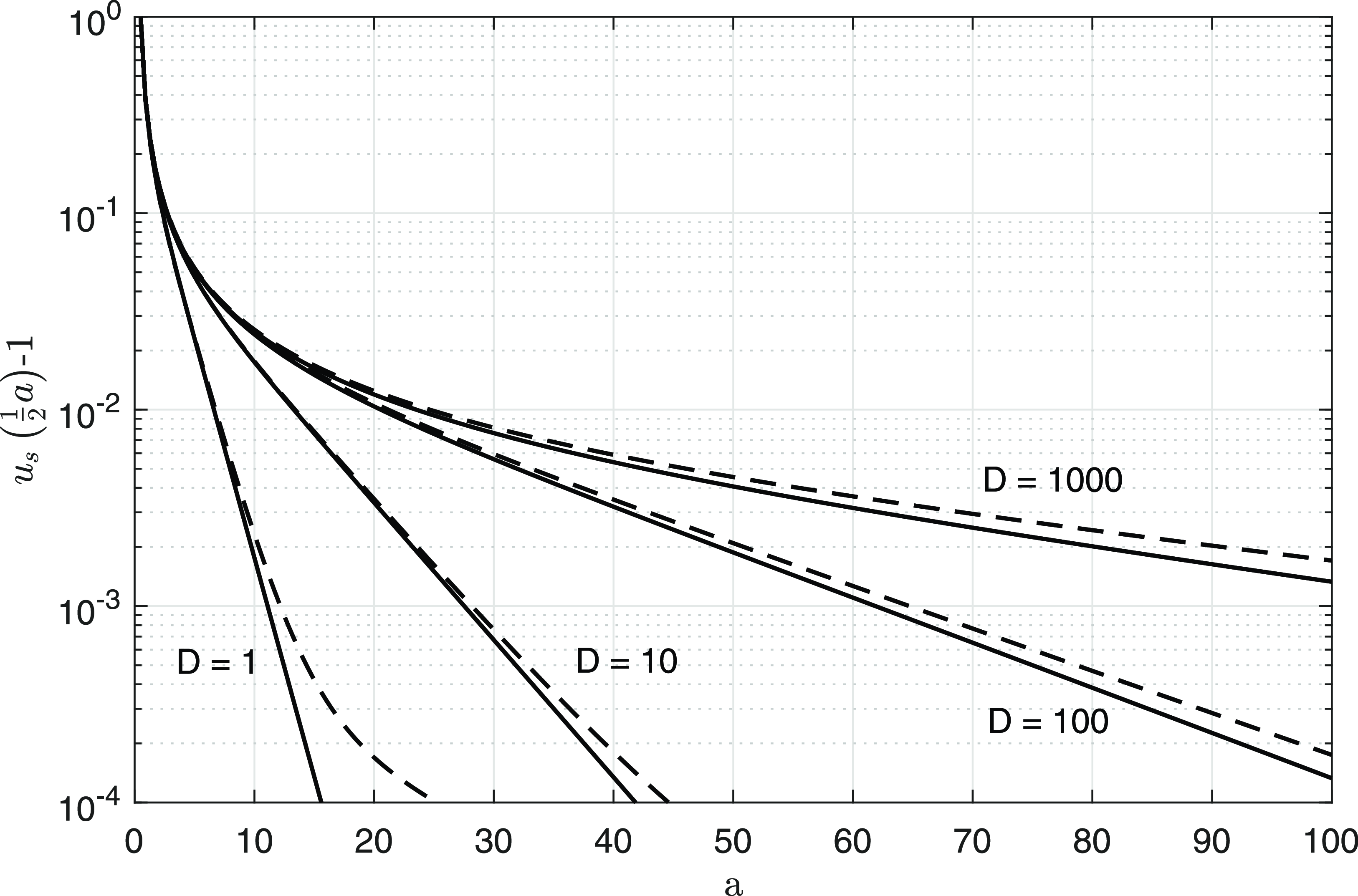
Figure 11. The value of the steady state at the midpoint of the domain (minus one for clarity), $u_s(\frac {1}{2}a) - 1$
, as a function of
$u_s(\frac {1}{2}a) - 1$
, as a function of $a\gt \frac {1}{2}$
for
$a\gt \frac {1}{2}$
for $D = 1$
,
$D = 1$
, $10$
,
$10$
, $100$
and
$100$
and $1000$
. The broken line is the leading order composite asymptotic approximation for
$1000$
. The broken line is the leading order composite asymptotic approximation for $D \gg 1$
, (104).
$D \gg 1$
, (104).
This completes the analysis and determination of the steady state structure when $D$
is large. We now consider the situation when
$D$
is large. We now consider the situation when $D=O(1)$
and
$D=O(1)$
and $a$
is large.
$a$
is large.
3.2.2.
$D=O(1)$
with
$a\gg 1$


In this case, the details are very similar to the corresponding case in section 2, as detailed in subsection 2.2.4, and so we can limit ourselves to presenting the salient results, which we have obtained from the full problem, again via construction through the application of the method of matched asymptotic expansions. For $D\ge \Delta _1$
, our asymptotic analysis demonstrates that there is a unique steady state at each large
$D\ge \Delta _1$
, our asymptotic analysis demonstrates that there is a unique steady state at each large $a$
, which has, in the bulk region,
$a$
, which has, in the bulk region,
 \begin{equation} u_s(x,D,a)\sim 1\,\,\text{as}\,\,a\to \infty \end{equation}
for $x\in (O(1)^+,a-O(1)^+)$
. However, for
$x\in (O(1)^+,a-O(1)^+)$
. However, for $0\lt D\lt \Delta _1$
, the existence of multi-peak steady states appears for
$0\lt D\lt \Delta _1$
, the existence of multi-peak steady states appears for $a$
large. In particular, for fixed
$a$
large. In particular, for fixed $D\lt \Delta _1$
, and each large integer
$D\lt \Delta _1$
, and each large integer $r$
, there is an
$r$
, there is an $r$
-peak nontrivial, non-negative steady state for each
$r$
-peak nontrivial, non-negative steady state for each $\lambda \in (\lambda _1^-(D),\lambda _1^+(D))$
, given by, in the bulk region,
$\lambda \in (\lambda _1^-(D),\lambda _1^+(D))$
, given by, in the bulk region,
 \begin{equation} u_s(x,D,a)\sim F_p(x+x_M(\lambda ,D),\lambda ,D), \end{equation}
for $x\in (O(1)^+,a-O(1)^+)$
, with corresponding
$x\in (O(1)^+,a-O(1)^+)$
, with corresponding $L^1$
norm being,
$L^1$
norm being,
 \begin{equation} ||u_s(\cdot ,D,a)||_1\sim rA(\lambda ,D) \end{equation}
and large $a$
given, in terms of
$a$
given, in terms of $\lambda$
, by
$\lambda$
, by
 \begin{equation} a = \lambda (r-1) + O(1)\,\,\text{as}\,\,r\to \infty , \end{equation}
for each $\lambda \in (\lambda _1^-(D),\lambda _1^+(D))$
. Here
$\lambda \in (\lambda _1^-(D),\lambda _1^+(D))$
. Here $x_M$
and
$x_M$
and $A$
are as given in (63) and (68), respectively. In the
$A$
are as given in (63) and (68), respectively. In the $(a,||u_s(\cdot ,D,a)||_1)$
bifurcation plane, for each large integer
$(a,||u_s(\cdot ,D,a)||_1)$
bifurcation plane, for each large integer $r$
, the associated family of
$r$
, the associated family of $r$
-peak steady states lies on an echelon above the interval with
$r$
-peak steady states lies on an echelon above the interval with $a\in I_r(D)$
(as given in (66)), parameterised by
$a\in I_r(D)$
(as given in (66)), parameterised by $\lambda \in (\lambda _1^-(D),\lambda _1^+(D))$
, via (107) and (108). Sequential echelons are again overlapping, and at a given large
$\lambda \in (\lambda _1^-(D),\lambda _1^+(D))$
, via (107) and (108). Sequential echelons are again overlapping, and at a given large $a$
, the overlapping echelons have those integer values, with
$a$
, the overlapping echelons have those integer values, with $r_m(a,D)\le r \le r_M(a,D)$
, as for the Dirichlet case. Also, for
$r_m(a,D)\le r \le r_M(a,D)$
, as for the Dirichlet case. Also, for $r$
large, each echelon has length of
$r$
large, each echelon has length of $O(r)$
and variation of
$O(r)$
and variation of $O(r)$
, and so slope of O(1), whilst each sequential echelon is lifted by
$O(r)$
, and so slope of O(1), whilst each sequential echelon is lifted by $O(1)$
with each unit increase in
$O(1)$
with each unit increase in $r$
. Again, in the bifurcation diagram, each sequential echelon is connected by a loop containing a supercritical and subcritical saddle-node bifurcation point, the traversal of which accommodates the transition from an
$r$
. Again, in the bifurcation diagram, each sequential echelon is connected by a loop containing a supercritical and subcritical saddle-node bifurcation point, the traversal of which accommodates the transition from an $r$
-peak to an
$r$
-peak to an $(r+1)$
-peak structure in the steady state. We next consider the case when
$(r+1)$
-peak structure in the steady state. We next consider the case when $D$
is small.
$D$
is small.
3.2.3.
$0\lt D\ll 1$

The case $0\lt D\ll 1$
is similar to the corresponding case for the Dirichlet problem dealt with in subsection 2.2.5, and we therefore present only the salient features of our asymptotic analysis here. For each
$0\lt D\ll 1$
is similar to the corresponding case for the Dirichlet problem dealt with in subsection 2.2.5, and we therefore present only the salient features of our asymptotic analysis here. For each $r=2,3,\ldots$
, we have constructed a branch of
$r=2,3,\ldots$
, we have constructed a branch of $r$
-peak nontrivial, non-negative steady states, for
$r$
-peak nontrivial, non-negative steady states, for
 \begin{equation} a\in \left (\frac {1}{2}(r-1),r-\frac {1}{2}\left (3-\sqrt {2}\right )\right ), \end{equation}
given by,
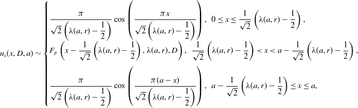 \begin{equation} u_s(x,D,a) \sim \begin{cases} \dfrac {\pi }{\sqrt {2}\left(\lambda (a,r)-\dfrac {1}{2}\right)}\cos \left (\dfrac {\pi x}{\sqrt {2}\left(\lambda (a,r)-\dfrac {1}{2}\right)}\right ),\,\,0\le x \le \dfrac {1}{\sqrt {2}}\left (\lambda (a,r)-\dfrac {1}{2}\right ),\\[12pt] F_p\left (x-\dfrac {1}{\sqrt {2}}\left(\lambda (a,r)-\dfrac {1}{2}\right),\lambda (a,r),D\right ),\,\,\dfrac {1}{\sqrt {2}}\left (\lambda (a,r)-\dfrac {1}{2}\right )\lt x\lt a-\dfrac {1}{\sqrt {2}}\left (\lambda (a,r)-\dfrac {1}{2}\right ),\\[12pt] \dfrac {\pi }{\sqrt {2}\left(\lambda (a,r)-\dfrac {1}{2}\right)}\cos \left (\dfrac {\pi (a-x)}{\sqrt {2}\left(\lambda (a,r)-\dfrac {1}{2}\right)}\right ) ,\,\,a-\dfrac {1}{\sqrt {2}}\left(\lambda (a,r)-\dfrac {1}{2}\right)\le x \le a, \end{cases} \end{equation}
as $D\to 0$
, with
$D\to 0$
, with
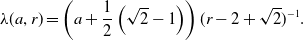 \begin{equation} \lambda (a,r) = \left (a + \frac {1}{2}\left (\sqrt {2}-1\right )\right ) (r - 2 + \sqrt {2})^{-1}. \end{equation}
Here, following (NB1), we have over one wavelength $\lambda$
, with
$\lambda$
, with $\lambda \in \left (\frac {1}{2},1\right )$
,
$\lambda \in \left (\frac {1}{2},1\right )$
,
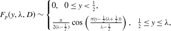 \begin{equation} F_p(y,\lambda ,D) \sim \begin{cases} 0,\,\,\,0 \le y \lt \frac {1}{2}, \\[5pt] \frac {\pi }{2(\lambda -\frac {1}{2})}\cos \left (\frac {\pi (y-\frac {1}{2}(\lambda +\frac {1}{2}))}{\lambda -\frac {1}{2}}\right ),\,\,\, \frac {1}{2}\le y\le \lambda , \end{cases} \end{equation}
as $D\to 0$
. Again, localised edge layers, of thickness
$D\to 0$
. Again, localised edge layers, of thickness $O(D^{\frac {1}{4}})$
, are present to smooth
$O(D^{\frac {1}{4}})$
, are present to smooth $F_p$
across the edge of its support regions in (112) (see section 4.1 in (NB1)). A notable and interesting feature of the
$F_p$
across the edge of its support regions in (112) (see section 4.1 in (NB1)). A notable and interesting feature of the $r$
-peak steady state in the Neumann case, given by (110), is that the peaks occurring at both end points have height and support width, which is exactly
$r$
-peak steady state in the Neumann case, given by (110), is that the peaks occurring at both end points have height and support width, which is exactly $\sqrt {2}$
times that of each interior peak. We are able to interpret this as being due to one half of the spatial extent of the boundary peak being clipped off beyond the boundary in relation to the nonlocal term in equation (1), whilst the edge layer requires that the slope at the edge of the boundary peak is equal to that at the edges of the interior peaks. This does not occur in the Dirichlet case, when all peaks have the same height in this limit. In the
$\sqrt {2}$
times that of each interior peak. We are able to interpret this as being due to one half of the spatial extent of the boundary peak being clipped off beyond the boundary in relation to the nonlocal term in equation (1), whilst the edge layer requires that the slope at the edge of the boundary peak is equal to that at the edges of the interior peaks. This does not occur in the Dirichlet case, when all peaks have the same height in this limit. In the $(a,||u_s||_1)$
bifurcation plane, the
$(a,||u_s||_1)$
bifurcation plane, the $r$
-peak echelon, for
$r$
-peak echelon, for $r=2$
,
$r=2$
, $3$
,
$3$
, $\ldots$
, is readily shown to have the curve given by,
$\ldots$
, is readily shown to have the curve given by,
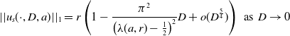 \begin{equation} ||u_s(\cdot ,D,a)||_1 = r\left (1 - \frac {\pi ^2}{\left (\lambda (a,r)-\frac {1}{2}\right )^2}D + o(D^{\frac {5}{4}})\right )\,\,\text{as}\,\,D\to 0 \end{equation}
for $a\in \left (\frac {1}{2}(r-1),(r-\frac {1}{2}\left (3-\sqrt {2}\right ))\right )$
. Finally, at each
$a\in \left (\frac {1}{2}(r-1),(r-\frac {1}{2}\left (3-\sqrt {2}\right ))\right )$
. Finally, at each $a\gt 1/2$
, there is an
$a\gt 1/2$
, there is an $r$
-peak steady state for each integer
$r$
-peak steady state for each integer $r$
satisfying
$r$
satisfying
 \begin{equation} r \in [1+a,1+2a]. \end{equation}
As in the Dirichlet case, on the $(a,||u_s||_1)$
bifurcation plane, each sequential echelon is connected by an elongated loop which has a low curvature supercritical saddle-node bifurcation at the lower end, and a high curvature subcritical saddle-node bifurcation at the upper end. A numerical illustration of the bifurcation plane, at
$(a,||u_s||_1)$
bifurcation plane, each sequential echelon is connected by an elongated loop which has a low curvature supercritical saddle-node bifurcation at the lower end, and a high curvature subcritical saddle-node bifurcation at the upper end. A numerical illustration of the bifurcation plane, at $D=10^{-5}$
, and obtained by solving the full problem, is given in Figure 12, along with the three steady state solutions when
$D=10^{-5}$
, and obtained by solving the full problem, is given in Figure 12, along with the three steady state solutions when $a = 2.75$
.
$a = 2.75$
.
Figure 12. The bifurcation diagram for (NIVP) with $D = 10^{-5}$
(left panel). The three stable steady states when
$D = 10^{-5}$
(left panel). The three stable steady states when $a = 2.75$
(indicated by the dotted line), with
$a = 2.75$
(indicated by the dotted line), with $r = 4$
,
$r = 4$
, $5$
and
$5$
and $6$
, are shown in the right-hand panel to illustrate the typical form of these steady states. Note the different scales on the
$6$
, are shown in the right-hand panel to illustrate the typical form of these steady states. Note the different scales on the $u_s$
-axes in the right-hand panels.
$u_s$
-axes in the right-hand panels.
This completes the analysis of nontrivial, non-negative steady states for small $D$
.
$D$
.
3.2.4.
$D=O(1)$
with
$a\gt 1/2$


Steady states, in this final case, are analysed via numerical pseudo-arclength continuation by fixing $D$
and then path following, from the unique nontrivial steady state at
$D$
and then path following, from the unique nontrivial steady state at $a=1/2$
, with increasing
$a=1/2$
, with increasing $a$
. The results are not qualitatively different to those that we obtained for the Dirichlet problem, and we have not added any new illustrations. The key conclusions from this numerical investigation follow directly those of subsection 2.2.6 for the Dirichlet case, and are therefore not repeated again in detail.
$a$
. The results are not qualitatively different to those that we obtained for the Dirichlet problem, and we have not added any new illustrations. The key conclusions from this numerical investigation follow directly those of subsection 2.2.6 for the Dirichlet case, and are therefore not repeated again in detail.
This completes the analysis of nontrivial, non-negative steady states for the Neumann problem when $a\gt 1/2$
. We note that the remarks concerning steady state hysteresis in section 2 relating to the Dirichlet case apply equally here. We are now in a position to consider the evolution problem (NIVP). At each
$a\gt 1/2$
. We note that the remarks concerning steady state hysteresis in section 2 relating to the Dirichlet case apply equally here. We are now in a position to consider the evolution problem (NIVP). At each $(a,D)\in (1/2,\infty )\times (0,\infty )$
, numerical solutions to (NIVP) approach one of the temporally stable nontrivial, non-negative steady states when
$(a,D)\in (1/2,\infty )\times (0,\infty )$
, numerical solutions to (NIVP) approach one of the temporally stable nontrivial, non-negative steady states when $t$
is large. As we saw for (DIVP), different initial conditions lead to different final steady states, but the behaviour of unsteady solutions to (NIVP) is not qualitatively different to those of (DIVP), and we need not present any further numerical illustrations.
$t$
is large. As we saw for (DIVP), different initial conditions lead to different final steady states, but the behaviour of unsteady solutions to (NIVP) is not qualitatively different to those of (DIVP), and we need not present any further numerical illustrations.
4. Conclusions
In this paper, we have considered evolution problems for the spatially nonlocal Fisher-KPP equation with simple top hat kernel, labelled as (DIVP), with Dirichlet boundary conditions, and (NIVP), with Neumann boundary conditions. The key feature of the inclusion of the nonlocal term is the introduction of a nonlocal length scale into the model. There are thus two dimensionless parameters in the model, namely $D$
, which measures the square of the ratio of the diffusion length scale (based on the kinetic time scale) to the nonlocal length scale, and
$D$
, which measures the square of the ratio of the diffusion length scale (based on the kinetic time scale) to the nonlocal length scale, and $a$
, which measures the ratio of the domain length scale to the nonlocal length scale. We have examined both the Dirichlet and the Neumann models for
$a$
, which measures the ratio of the domain length scale to the nonlocal length scale. We have examined both the Dirichlet and the Neumann models for $(a,D)$
throughout the positive quadrant of the parameter plane. Significant structural differences in behaviour between the classical Fisher-KPP model and this natural nonlocal extension have been identified, and these become more significant as the parameter
$(a,D)$
throughout the positive quadrant of the parameter plane. Significant structural differences in behaviour between the classical Fisher-KPP model and this natural nonlocal extension have been identified, and these become more significant as the parameter $D$
decreases. These principal, and marked, differences have been fully explored and exposed. The structural differences have included the existence of multiple, temporally stable, multipeak, nontrivial and non-negative steady states, accumulated through multiple steady state saddle-node bifurcations, with this giving rise to hysteretic behaviour with increasing and decreasing domain size
$D$
decreases. These principal, and marked, differences have been fully explored and exposed. The structural differences have included the existence of multiple, temporally stable, multipeak, nontrivial and non-negative steady states, accumulated through multiple steady state saddle-node bifurcations, with this giving rise to hysteretic behaviour with increasing and decreasing domain size $a$
, at sufficiently small
$a$
, at sufficiently small $D$
. In addition, the temporally stable multipeak steady states, when available, are shown to be large-
$D$
. In addition, the temporally stable multipeak steady states, when available, are shown to be large- $t$
attractors for the evolution problems (DIVP) and (NIVP), respectively. Although the details for (DIVP) and (NIVP) are broadly similar in key features, as highlighted in the relevant parts of section 3 and section 4, there are a number of interesting differences between the details of the two models, which should be highlighted. First, the trivial equilibrium state is universally unstable throughout the
$t$
attractors for the evolution problems (DIVP) and (NIVP), respectively. Although the details for (DIVP) and (NIVP) are broadly similar in key features, as highlighted in the relevant parts of section 3 and section 4, there are a number of interesting differences between the details of the two models, which should be highlighted. First, the trivial equilibrium state is universally unstable throughout the $(a,D)$
parameter space for (NIVP), but conditional on
$(a,D)$
parameter space for (NIVP), but conditional on $0\lt D\lt a^2/\pi ^2$
for (DIVP). In addition, when the trivial equilibrium state is unstable and
$0\lt D\lt a^2/\pi ^2$
for (DIVP). In addition, when the trivial equilibrium state is unstable and $D\lt \Delta _1$
, both models can support an accumulating number of non-negative multi-peak steady states, which have a broadly similar structure; however, a simple and clear distinguished difference, which appears when
$D\lt \Delta _1$
, both models can support an accumulating number of non-negative multi-peak steady states, which have a broadly similar structure; however, a simple and clear distinguished difference, which appears when $D$
becomes sufficiently small, and is evident in both the small
$D$
becomes sufficiently small, and is evident in both the small $D$
asymptotic theory and the numerical solutions of the full problem at small
$D$
asymptotic theory and the numerical solutions of the full problem at small $D$
, is that for the multi-peak steady states of (DIVP), all the peaks have approximately the same peak height and width, whilst for (NIVP), the two boundary peaks are exceptional in that they have a larger peak height, by a factor of
$D$
, is that for the multi-peak steady states of (DIVP), all the peaks have approximately the same peak height and width, whilst for (NIVP), the two boundary peaks are exceptional in that they have a larger peak height, by a factor of $\sqrt {2}$
, and a proportionately smaller peak width relative to each of the interior peaks, so that each peak encloses the same area.
$\sqrt {2}$
, and a proportionately smaller peak width relative to each of the interior peaks, so that each peak encloses the same area.
More generally, this paper and (NB1) have both studied a natural extension of the classical Fisher-KPP model, with the introduction of the simplest possible nonlocal effect into the saturation term. The motivation for these detailed analyses arises since nonlocal reaction-diffusion models occur naturally in a variety of (frequently biological or ecological) contexts, and as such it is of fundamental interest to examine the properties of the nonlocal Fisher-KPP model in detail, and to compare and contrast these with the well known properties of the classical Fisher-KPP model. As we have seen here, in (NB1) and in the work of many other authors (for example, [Reference Berestycki, Nadin, Perthame and Ryzhik3, Reference Billingham4, Reference Faye and Holzer8, Reference Gourley10, Reference Nadin, Perthame and Tang15, Reference Perthame and Génieys17]), the introduction of a nonlocal kernel leads to a huge increase in the complexity of possible solutions and their bifurcation structure. This has implications for the behaviour of nonlocal biological systems that are confined to a finite region, with a richer variety of spatial patterns possible than for systems with purely local interactions.
Since a top hat kernel is the simplest possible compactly-supported kernel, the detailed analysis that we present here and in (NB1) forms the basis for an investigation into the form of solutions when the kernel is not constant on its support. Our ongoing investigation suggests that adding a small variation to the kernel is, in the limit $D \to 0$
, a singular perturbation, and that unravelling the bifurcation structure, starting from the structure presented here for the top hat kernel, will reveal a wide variety of additional solution branches. This will be the subject of a subsequent paper.
$D \to 0$
, a singular perturbation, and that unravelling the bifurcation structure, starting from the structure presented here for the top hat kernel, will reveal a wide variety of additional solution branches. This will be the subject of a subsequent paper.
Competing interests
None.
A. Numerical methods
A.1. Finite difference discretisation
All of the numerical methods that we use in this paper are based on central finite differences in space for second derivatives and the trapezium rule for the convolution integral. We discretise at $N$
equally-spaced points,
$N$
equally-spaced points, $x_i$
, in
$x_i$
, in $[0,a]$
, with
$[0,a]$
, with $x_0=0$
and
$x_0=0$
and $x_N = a$
. The trapezium rule that we use for the convolution integral respects the fact that the end points,
$x_N = a$
. The trapezium rule that we use for the convolution integral respects the fact that the end points, $\alpha (x)$
and
$\alpha (x)$
and $\beta (x)$
, defined in (4) and (5), may fall between two grid points, and is calculated based on a linear variation of
$\beta (x)$
, defined in (4) and (5), may fall between two grid points, and is calculated based on a linear variation of $u$
between grid points. This is used in the discretisation of both the steady and unsteady versions of (1) and the stability problem described in Appendix B. The Neumann boundary conditions, (8), are discretised using a three point difference formula in order to maintain second order accuracy in space. We typically used
$u$
between grid points. This is used in the discretisation of both the steady and unsteady versions of (1) and the stability problem described in Appendix B. The Neumann boundary conditions, (8), are discretised using a three point difference formula in order to maintain second order accuracy in space. We typically used $N=1000$
.
$N=1000$
.
A.2. Pseudo-arclength continuation
We investigate the bifurcation diagram for the steady states, $u_s(x)$
, of (1) using pseudo-arclength continuation, [Reference Allgower and Georg1], in
$u_s(x)$
, of (1) using pseudo-arclength continuation, [Reference Allgower and Georg1], in $(a, ||u_1||_1)$
parameter space. We will use the notation
$(a, ||u_1||_1)$
parameter space. We will use the notation $A \equiv ||u_s||_1$
below for clarity. The discretised linear system that arises from (1) with
$A \equiv ||u_s||_1$
below for clarity. The discretised linear system that arises from (1) with $u_t=0$
and either Dirichlet or Neumann boundary conditions is supplemented by the conditions
$u_t=0$
and either Dirichlet or Neumann boundary conditions is supplemented by the conditions
 \begin{equation} \left (a-a_0\right )^2 + \left (A-A_0\right )^2 = ds^2, \end{equation}
and
 \begin{equation} \int _0^a u_s(x) dx = A, \end{equation}
with the trapezium rule used to evaluate this integral. Here, $a_0$
and
$a_0$
and $A_0$
are the values of the length of the domain and the area under the solution at the previous point on the solution curve, and
$A_0$
are the values of the length of the domain and the area under the solution at the previous point on the solution curve, and $ds$
is the pseudo-arclength that we attempt to traverse in the
$ds$
is the pseudo-arclength that we attempt to traverse in the $(a,A) \equiv (a, ||u_s||_1)$
parameter space. The nonlinear system of algebraic equations that determine the discretised solution is solved using ‘fsolve’ in MATLAB, with the Jacobian of the system supplied analytically. The initial discrete solution is determined for
$(a,A) \equiv (a, ||u_s||_1)$
parameter space. The nonlinear system of algebraic equations that determine the discretised solution is solved using ‘fsolve’ in MATLAB, with the Jacobian of the system supplied analytically. The initial discrete solution is determined for $a \lt \frac {1}{2}$
, in which case a simple analytical solution is available for both (DIVP) and (NIVP). Linear extrapolation is used to obtain new guesses of
$a \lt \frac {1}{2}$
, in which case a simple analytical solution is available for both (DIVP) and (NIVP). Linear extrapolation is used to obtain new guesses of $a$
and
$a$
and $A$
, and we use a simple scaling factor for
$A$
, and we use a simple scaling factor for $ds$
so that it is reduced when the solution fails to converge and increased otherwise, with
$ds$
so that it is reduced when the solution fails to converge and increased otherwise, with $10^{-6} \leq ds \leq 5 \times 10^{-3}$
. For
$10^{-6} \leq ds \leq 5 \times 10^{-3}$
. For $D$
sufficiently large, specifically
$D$
sufficiently large, specifically $D\gt 10^{-3}$
, this method is sufficient to calculate the bifurcation diagrams presented in the paper, including the loops in parameter space shown in Figure 7.
$D\gt 10^{-3}$
, this method is sufficient to calculate the bifurcation diagrams presented in the paper, including the loops in parameter space shown in Figure 7.
For smaller values of $D$
, the curvature of the saddle node bifurcation at the right of each loop becomes so large that this algorithm fails. It seems likely that this curvature becomes exponentially large as
$D$
, the curvature of the saddle node bifurcation at the right of each loop becomes so large that this algorithm fails. It seems likely that this curvature becomes exponentially large as $D \to 0$
, in effect forming a cusp at which the direction of the bifurcation curve reverses at the bifurcation, which is too much for our simple algorithm to cope with. We overcome this by using parameter continuation to generate a solution on the stable branch above the cusp and then use pseudo-arclength continuation to reach the cusp from the opposite direction. This is sufficient to generate all of the bifurcation diagrams in the paper. At all values of
$D \to 0$
, in effect forming a cusp at which the direction of the bifurcation curve reverses at the bifurcation, which is too much for our simple algorithm to cope with. We overcome this by using parameter continuation to generate a solution on the stable branch above the cusp and then use pseudo-arclength continuation to reach the cusp from the opposite direction. This is sufficient to generate all of the bifurcation diagrams in the paper. At all values of $D$
for which bifurcation loops occur, when
$D$
for which bifurcation loops occur, when $a$
becomes sufficiently large the curvature of the saddle-node bifurcation at the left of the loop also becomes too tight for our algorithm to cope with, but we have not attempted to deal with this problem as the results presented in the paper are sufficient to illustrate the form of the bifurcation diagram.
$a$
becomes sufficiently large the curvature of the saddle-node bifurcation at the left of the loop also becomes too tight for our algorithm to cope with, but we have not attempted to deal with this problem as the results presented in the paper are sufficient to illustrate the form of the bifurcation diagram.
A.3. Numerical solution of (DIVP) and (NIVP)
After discretising (DIVP) and (NIVP) in space using the finite difference method described in Appendix A.1, we use the midpoint method to evolve the solution from its initial state. If we write the discretised system as $\dot {\textbf{u}} = \textbf{F}(\textbf{u})$
, with
$\dot {\textbf{u}} = \textbf{F}(\textbf{u})$
, with $u_i = u(x_i,t)$
, this is
$u_i = u(x_i,t)$
, this is
 \begin{equation*} \bar {\textbf{u}}(t) = \textbf{u}(t) + \frac {1}{2}\Delta t \, \textbf{F}(\textbf{u}(t)),\,\,\,\textbf{u}(t+\Delta t) = \textbf{u}(t) + \Delta t \, \textbf{F}(\bar {\textbf{u}}(t)). \end{equation*}
We choose a time step, $\Delta t$
, adaptively so that the maximum change in
$\Delta t$
, adaptively so that the maximum change in $u$
is less than
$u$
is less than $10^{-4}$
, with maximum time step
$10^{-4}$
, with maximum time step $\frac {1}{4} D^{-1} \Delta x^2$
.
$\frac {1}{4} D^{-1} \Delta x^2$
.
B. Linear stability of steady states
To determine the linear stability property of the steady state $u_s$
, we define a new dependent variable
$u_s$
, we define a new dependent variable $\hat {u}(x)$
by
$\hat {u}(x)$
by
 \begin{equation*}u= u_s(x) + \hat {u}(x) e^{\sigma t},\end{equation*}
substitute into (DIVP) and (NIVP), and assume that $|\hat {u}| \ll 1$
, to obtain the linear stability problem
$|\hat {u}| \ll 1$
, to obtain the linear stability problem
 \begin{equation} D \hat {u}'' + \left (1 - \int _{\alpha (x)}^{\beta (x)} u_s(y)dy\right ) \hat {u} - u_s(x) \int _{\alpha (x)}^{\beta (x)} \hat {u}(y)dy = \sigma \hat {u},\,\,x\in (0,a), \end{equation}
subject to the boundary conditions
 \begin{equation} \hat {u}(0) = \hat {u}(a) = 0, \end{equation}
for (DIVP), and
 \begin{equation} \hat {u}'(0) = \hat {u}'(a) = 0, \end{equation}
for (NIVP). It is straightforward to discretise this linear eigenvalue problem using the finite difference approach described in Appendix A.1. The resulting matrix eigenvalue problem can then be solved in MATLAB using the built-in routine ‘eig’. This determines that the eigenvalues are real and typical results for the largest eigenvalue as a function of $a$
for fixed
$a$
for fixed $D$
are shown in Figures 8 and 9.
$D$
are shown in Figures 8 and 9.


 Open access