


1 Introduction
In this paper, we consider pattern formation in a particular system of partial differential equations (PDEs) with fractional Laplacian, where a Ginzburg–Landau equation is coupled with a mean field. We consider the following fractional amplitude equations with periodic boundary conditions:
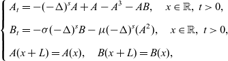 \begin{equation}\left\{\begin{aligned}&A_t=-(-\Delta)^sA+A-A^3-AB,\quad x\in \mathbb{R},\ t>0,\\[5pt]&B_t=-\sigma(-\Delta)^s B-\mu (-\Delta)^s(A^2),\quad x\in \mathbb{R},\ t>0,\\[5pt]&A(x+L)=A(x),\quad B(x+L)=B(x),\end{aligned}\right.\end{equation}
where
 \begin{equation*}\sigma>0,\quad \mu\in \mathbb{R}\quad \mbox{and}\quad L \mbox{is the minimal period}.\end{equation*}
We assume the exponent satisfies $1/2<s<1$
. The fractional Laplacian
$1/2<s<1$
. The fractional Laplacian $(-\Delta)^s$
replaces the classical Laplacian as the infinitesimal generator of the underlying Lévy process and is defined by:
$(-\Delta)^s$
replaces the classical Laplacian as the infinitesimal generator of the underlying Lévy process and is defined by:
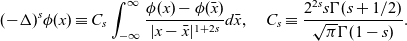 \begin{equation*}(-\Delta)^s\phi(x)\equiv C_s\int_{-\infty}^{\infty}\frac{\phi(x)-\phi(\bar{x})}{|x-\bar{x}|^{1+2s}}d\bar{x},\quad C_s \equiv \frac{2^{2s}s\Gamma(s+1/2)}{\sqrt{\pi}\Gamma(1-s)}.\end{equation*}
By taking $\tau=1/\sigma,\mu{'}=\mu/\sigma$
, equation (1.1) can be rewritten in the form:
$\tau=1/\sigma,\mu{'}=\mu/\sigma$
, equation (1.1) can be rewritten in the form:
 \begin{equation}\left\{\begin{aligned}&A_t=-(-\Delta)^sA+A-A^3-AB,\quad x\in \mathbb{R},\ t>0,\\[5pt]&\tau B_t=-(-\Delta)^s B-\mu{'}(-\Delta)^s (A^2),\quad x\in \mathbb{R},\ t>0,\\[5pt]\end{aligned}\right.\end{equation}
It is easy to see that the equation (1.2) is invariant if
 \begin{equation*}A \mbox{ transforms to }-A\quad \mbox{or if}\quad x \mbox{ transforms to }-x.\end{equation*}
Systems with a conservation law frequently arise as models in fluid mechanics, chemistry or biology. The resulting solutions often describe various types of pattern formation. As a prototype example, equation (1.1) arises in the study of the following PDE:
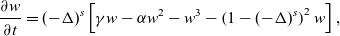 \begin{equation}\frac{\partial w}{\partial t}=(-\Delta)^s\left[\gamma w- \alpha w^2-w^3-\left(1-(-\Delta)^s\right)^2 w\right],\end{equation}
where the terms inside the brackets are the same as in the Swift–Hohenberg equation [Reference Swift and Hohenberg23] with fractional Laplacian, supplemented with a symmetry-breaking quadratic term $-\alpha w^2$
. The symmetry-breaking term is necessary for the amplitude equations to become a system as in (1.1). In case
$-\alpha w^2$
. The symmetry-breaking term is necessary for the amplitude equations to become a system as in (1.1). In case $\alpha=0$
, we would obtain a Ginzburg–Landau equation without a mean field. Note that the PDE (1.3) has the following essential features:
$\alpha=0$
, we would obtain a Ginzburg–Landau equation without a mean field. Note that the PDE (1.3) has the following essential features:
-
• It possesses conserved quantities. In a sense, it is a conservation law.
-
• It is a parabolic equation with fractional Laplacian at lowest order in w.
-
• It has the symmetry groups $x\to -x$
and
$x\to x+x_0$
for all
$x_0\in \mathbb{R}$
.
$x\to -x$
and
$x\to x+x_0$
for all
$x_0\in \mathbb{R}$
. -
• It arises in the perturbation analysis near a cubic bifurcation point in the supercritical case.
-
• The Fourier modes
$e^{i0x}$
and
$e^{\pm ix}$
are neutrally stable at the bifurcation point
$\gamma=0,\,w=0$
. -
• For
$0<\gamma<1$
and
$\frac{1}{2}<s<1$
, the growth rate
$\lambda$
of mode k for (1.3) is given by: Note that
\begin{equation*} \lambda=|k|^{2s}[\gamma-(1-|k|^{2s})^2]. \end{equation*}
$\lambda=0$
for
$k=0$
and
$|k|=(1\pm\sqrt{\gamma})^{1/2s}.$


Extending the approach of [Reference Matthews and Cox13] from the case $s=1$
to
$s=1$
to $\frac{1}{2}<s<1$
by suitable rescaling, we next show that the equations (1.1) arise as amplitude equations of (1.3). To this end, we make the ansatz
$\frac{1}{2}<s<1$
by suitable rescaling, we next show that the equations (1.1) arise as amplitude equations of (1.3). To this end, we make the ansatz
 \begin{equation} \gamma=\varepsilon^{2s} \gamma_1, \quad T=\varepsilon^{2s} t, \quad X=\varepsilon x,\end{equation}
and
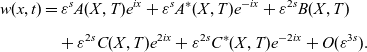 \begin{equation} \begin{aligned} w(x,t)&= \varepsilon^s A(X,T)e^{ix}+\varepsilon^s A^*(X,T) e^{-ix}+\varepsilon^{2s} B(X,T)\\[5pt] & \quad + \varepsilon^{2s} C(X, T) e^{2 i x} + \varepsilon^{2s} C^{*} (X, T) e^{-2i x} + O(\varepsilon^{3s}). \end{aligned}\end{equation}
Note that in the expansion of w, at leading order $\varepsilon^s$
there is a large-scale oscillation A (and its complex conjugate
$\varepsilon^s$
there is a large-scale oscillation A (and its complex conjugate $A^*$
). The mode B, which has been introduced at order
$A^*$
). The mode B, which has been introduced at order $\varepsilon^{2s}$
, is constant on the large spatial scale.
$\varepsilon^{2s}$
, is constant on the large spatial scale.
We substitute (1.5) into (1.3) and then solve the equations at successive orders of $\varepsilon$
. First, in order
$\varepsilon$
. First, in order $\varepsilon^{2s}$
we derive
$\varepsilon^{2s}$
we derive
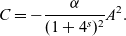 \begin{equation*}C=-\frac{\alpha}{(1+4^s)^2}A^2.\end{equation*}
Then, the following equations are established:
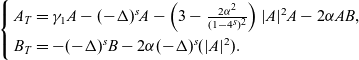 \begin{align} \left\{ \begin{array}{l} A_T= \gamma_1 A - (-\Delta)^s A - \left(3-\frac{2\alpha^2}{(1-4^s)^2}\right) |A|^2 A -2\alpha AB, \\[5pt] B_T=-(-\Delta)^s B - 2 \alpha (-\Delta)^s(|A|^2). \end{array} \right. \end{align}
The equation (1.6) arises in order $\varepsilon^{3s}$
, where A is complex-valued. The equation (1.6) is shown by equating terms of order
$\varepsilon^{3s}$
, where A is complex-valued. The equation (1.6) is shown by equating terms of order $\varepsilon^{4s}$
. In this paper, we restrict our attention to the invariant subspace in which A is real. Therefore, from now on, we consider the special case that A is real. By rescaling
$\varepsilon^{4s}$
. In this paper, we restrict our attention to the invariant subspace in which A is real. Therefore, from now on, we consider the special case that A is real. By rescaling $A,\,B,\,T\,$
and X, we can make all coefficients in equation (1.6) equal to unity, and we get (1.1).
$A,\,B,\,T\,$
and X, we can make all coefficients in equation (1.6) equal to unity, and we get (1.1).
Amplitude equations of the form (1.2) or conservative models of the form (1.3) have been considered in hydrodynamics in the case of the classical Laplacian. See for instance, [Reference Fauve7]. We also refer to [Reference Cox and Matthews5] and [Reference Matthews and Cox13], where (1.2) was derived from non-linear PDEs in the classical Laplacian case which arise in thermosolutal convection, rotating convection or magnetoconvection, respectively. Furthermore, in [Reference Coullet and Iooss4], the equation (1.2) was also derived in the study of secondary stability of a one-dimensional cellular pattern for the classical Laplacian. A related kind of Ginzburg–Landau equation, where the term $(|A|^2)_{xx}$
in the B-equation is replaced by
$(|A|^2)_{xx}$
in the B-equation is replaced by $ \partial_x (|A|^2)$
has been studied by a number of authors in the classical Laplacian case, see [Reference Riecke20], [Reference Riecke and Rappel21] and the references therein. The most common patterns occurring in that setting are travelling pulses which arise in the convection of binary fluids. In [Reference Tribelsky and Tsuboi24], a conserved variant of (1.3) for
$ \partial_x (|A|^2)$
has been studied by a number of authors in the classical Laplacian case, see [Reference Riecke20], [Reference Riecke and Rappel21] and the references therein. The most common patterns occurring in that setting are travelling pulses which arise in the convection of binary fluids. In [Reference Tribelsky and Tsuboi24], a conserved variant of (1.3) for $s=1$
has been considered which has the same linear dispersion relation but different non-linear behaviour. In this case, the behaviour becomes chaotic. In recent years, fractional diffusion systems have been investigated in fluid mechanics to model, analyse and compute the road to turbulence [Reference Chen3, Reference Gunzburger, Jiang and Xu11, Reference Samiee, Akhavan-Safaei and Zayernouri22] and also used in the study of pattern formation in reaction–diffusion systems, such as the fractional Gierer–Meinhardt system, see [Reference Gomez, Wei and Yang9, Reference Medeiros, Wei and Yang15] and the references therein.
$s=1$
has been considered which has the same linear dispersion relation but different non-linear behaviour. In this case, the behaviour becomes chaotic. In recent years, fractional diffusion systems have been investigated in fluid mechanics to model, analyse and compute the road to turbulence [Reference Chen3, Reference Gunzburger, Jiang and Xu11, Reference Samiee, Akhavan-Safaei and Zayernouri22] and also used in the study of pattern formation in reaction–diffusion systems, such as the fractional Gierer–Meinhardt system, see [Reference Gomez, Wei and Yang9, Reference Medeiros, Wei and Yang15] and the references therein.
We shall study equation (1.2) with the following periodic boundary conditions which arise from the expansion (1.4) and (1.5):
 \begin{equation}A(x+L)=A(x), \quad B(x+L)=B(x),\end{equation}
where L is the minimal period. Other boundary conditions may be more appropriate for other modelling situations. We now present our two main results on the existence and stability of stationary patterns for system (1.2).
Theorem 1.1. There exists an $\bar{L}>0$
such that for all
$\bar{L}>0$
such that for all $L>\bar{L}$
, system (1.2) admits the following three types of steady-state solutions.
$L>\bar{L}$
, system (1.2) admits the following three types of steady-state solutions.
Type I (Double-front solution). Assume that $\mu{'}<1$
. Then there exist (even) steady-state solutions of (1.2) with the following asymptotic behaviour:
$\mu{'}<1$
. Then there exist (even) steady-state solutions of (1.2) with the following asymptotic behaviour:
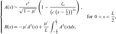 \begin{equation*} \left\{ \begin{aligned} & A(x)\sim \frac{c^s}{\sqrt{1-\mu{'}}}\left(1-\frac{\zeta_s}{\left(c\left(x-\frac{L}{4}\right)\right)^{2s}}\right), \\[5pt] & B(x)=-\mu{'}A^2(x)+\frac{\mu{'}}{L}\int_{-\frac{L}{2}}^{\frac{L}{2}}A^2(x)dx,\end{aligned} \quad \mbox{for}\,0<x<\frac{L}{2},\right. \end{equation*}
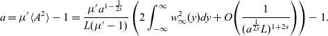
where c is the positive root of the following algebraic equation:
 \begin{equation*}c^{2s}+\frac{2\mu{'}\mathrm{I}_{v_\infty}}{L}c^{2s-1}-(1-\mu{'})=0\quad\textrm{and}\quad \mathrm{I}_{v_\infty}=\int_{\mathbb{R}}(v_\infty^2(y)-1)dy.\end{equation*}
Here, $v_\infty$
satisfies (2.6).
$v_\infty$
satisfies (2.6).
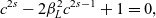
Type II (Single-spike solution). Assume that
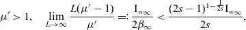 \begin{equation}\mu{'}>1,\quad\lim\limits_{L\to\infty}\frac{L(\mu{'}-1)}{\mu{'}}=: \frac{\mathrm{I}_{w_\infty}}{2\beta_\infty}<\frac{(2s-1)^{1-\frac{1}{2s}}\mathrm{I}_{w_\infty}}{2s},\end{equation}
where
 \begin{equation*}\mathrm{I}_{w_\infty}=\int_{\mathbb{R}}w_\infty^2(y)dy,\end{equation*}
and $w_\infty(y)$
is defined in (2.8). Then there exist steady-state solutions of (1.2) with the following asymptotic behaviour:
$w_\infty(y)$
is defined in (2.8). Then there exist steady-state solutions of (1.2) with the following asymptotic behaviour:
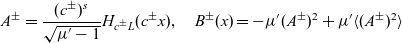
 \begin{equation*}A^{\pm}(x) \sim \frac{(c^{\pm})^s}{\sqrt{\mu{'}-1}}\frac{\xi_s}{1+|c^\pm x|^{1+2s}},\quad B^\pm (x)=-\mu{'}(A^\pm)^2+\frac{\mu{'}}{L}\int_{-L/2}^{L/2}(A^\pm)^2dx,\end{equation*}
where $c^-<c^+$
are the two roots of the following algebraic equation:
$c^-<c^+$
are the two roots of the following algebraic equation:
 \begin{equation*}c^{2s}-2\beta_\infty c^{2s-1}+1=0.\end{equation*}
Type III (Double-spike solution). Assume that
 \begin{equation} \mu{'}>1,\quad \lim\limits_{L\to\infty}\frac{L(\mu{'}-1)}{\mu{'}}=: \frac{\mathrm{I}_{w_\infty}}{2\beta_\infty}<\frac{(2s-1)^{1-\frac{1}{2s}}\mathrm{I}_{w_\infty}}{s}.\end{equation}
Then there exist steady-state solutions of (1.2) with the following asymptotic behaviour:
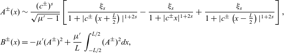 \begin{equation*} \begin{aligned} &A^{\pm}(x) \sim \frac{(c^{\pm})^s}{\sqrt{\mu{'}-1}}\left[\frac{\xi_s}{1+|c^\pm \left(x+\frac{L}{2}\right)|^{1+2s}}-\frac{\xi_s}{1+|c^\pm x|^{1+2s}}+\frac{\xi_s}{1+|c^\pm \left(x-\frac{L}{2}\right)|^{1+2s}}\right],\\[5pt] &B^\pm (x)=-\mu{'}(A^\pm)^2+\frac{\mu{'}}{L}\int_{-L/2}^{L/2}(A^\pm)^2dx, \end{aligned}\end{equation*}
where $c^-<c^+$
are the two roots of the following algebraic equation:
$c^-<c^+$
are the two roots of the following algebraic equation:
 \begin{equation*} c^{2s}-4\beta_\infty c^{2s-1}+1=0.\end{equation*}
Our next theorem classifies the stability of all the three types of solutions given in Theorem 1.1.
Theorem 1.2. Suppose that $L\gg 1$
and
$L\gg 1$
and $\tau>0$
. Then, for the single-spike solution (Type II),
$\tau>0$
. Then, for the single-spike solution (Type II), $(A^-,B^-)$
is linearly stable, while
$(A^-,B^-)$
is linearly stable, while $(A^+,B^+)$
is linearly unstable. The double-front solutions (Type I) and the double-spike solutions (Type III) are all linearly unstable.
$(A^+,B^+)$
is linearly unstable. The double-front solutions (Type I) and the double-spike solutions (Type III) are all linearly unstable.
Let us close the introduction by mentioning the new contribution of the current paper. Particularly, in the proof of Theorem 1.2, to show that the double-front solution (Type I) is unstable, the crucial point is to find a suitable test function. Following the approach of the classical case in [Reference Norbury, Wei and Winter19], we have to verify that the test function indeed satisfies the required boundary condition. Unlike in the classical case, we cannot use the ODE uniqueness theory to justify the sign condition of the derivative at the end point. Instead, we utilise the integral representation of the fractional Laplacian to achieve this goal. This part is inspired by the argument used for deriving the version of Hopf boundary lemma for fractional Laplacian, see [Reference Li and Chen12] for the details. We remark that Type I double-front solutions have also been analysed in Section 3 of [Reference Nec, Nepomnyashchy and Golovin18] in a similar context.
The paper is organised as follows: in Section 2, we present some preliminary results which are used in this paper. Further, Sections 3 and 4 are devoted to giving the proof of Theorem 1.1 and Theorem 1.2, respectively. In Section 5, we apply two numerical schemes to compute the shapes of the stable steady-state solutions with s at some specific values, and some pictures of simulations are presented. In last section, we give the concluding remarks.
Notations:
-
$w_\infty$
$w_\infty$
is the positive spike solution of (2.8).
-
$\mathrm{I}_{w_\infty}$
The integral value of
$\int_{\mathbb{R}}w^2_\infty dx$
.
-
$v_\infty$
$v_\infty$
is the layer solution of the fractional Allen–Cahn equation satisfying (2.6).
-
$\mathrm{I}_{v_\infty}$
The integral value of
$\int_{\mathbb{R}}(v^2_\infty-1) dx$
.
-
C a generic positive constant, which may change from line to line.


2 Preliminaries
2.1 Existence analysis
Consider the steady states of the equations (1.2):
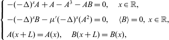 \begin{align} \left\{ \begin{array}{l} -(-\Delta)^sA+A-A^3-AB=0,\quad x\in \mathbb{R}, \\[5pt] -(-\Delta)^s B-\mu{'}(-\Delta)^s(A^2)=0,\quad \langle B \rangle=0,\, x\in \mathbb{R}, \\[5pt] A(x+L)=A(x),\quad B(x+L)=B(x), \end{array} \right. \end{align}
where $\langle B \rangle$
is the average of the function B over the minimal period, defined by:
$\langle B \rangle$
is the average of the function B over the minimal period, defined by:
 \begin{equation*}\langle B \rangle=\frac{1}{L}\int_{I}B(x)dx.\end{equation*}
Note that by adding a constant to B, (1.2) can be reduced to (2.1). Without loss of generality, we may assume that the minimal period interval is $I := [-L/2,L/2]$
.
$I := [-L/2,L/2]$
.
From the equation (2.1), we obtain that
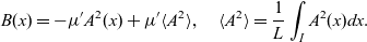 \begin{equation}B(x)=-\mu{'}A^2(x)+\mu{'}\langle A^2\rangle, \quad \langle A^2\rangle=\frac{1}{L}\int_{I}A^2(x)dx.\end{equation}
Substituting (2.2) into (2.1), we obtain
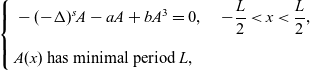 \begin{equation}\left\{\begin{aligned}& -(-\Delta)^sA-aA+bA^3=0, \quad -\frac{L}{2}<x<\frac{L}{2},\\[5pt]& A(x) \mbox{ has minimal period } L,\end{aligned}\right.\end{equation}
where
 \begin{equation}a=\mu{'}\langle A^2\rangle-1,\quad b=\mu{'}-1.\end{equation}
We consider a as a real parameter. Since (2.3) is an autonomous equation, we may assume that A satisfies the following boundary, symmetry and monotonicity conditions:
 \begin{equation}A'\!\left(-\frac{L}{2}\right)= A'\!\left(\frac{L}{2}\right)=0,\quad A(x)=A(-x),\quad A'(x)<0,\quad \mbox{for } 0<x<\frac{L}{2}.\end{equation}
It is interesting to remark that a periodic solution A of (2.3) satisfying (2.5) for $-L/2<x<L/2$
can be extended in a unique way to a periodic function on the real line with minimal period L.
$-L/2<x<L/2$
can be extended in a unique way to a periodic function on the real line with minimal period L.
To describe the possible asymptotic behaviour of A as $L\to +\infty$
, we introduce two standard limiting equations. The first one is a forward front on
$L\to +\infty$
, we introduce two standard limiting equations. The first one is a forward front on $\mathbb{R}$
. Suppose that
$\mathbb{R}$
. Suppose that $v_\infty$
is the solution of the following problem:
$v_\infty$
is the solution of the following problem:
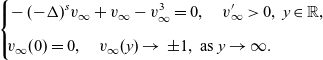 \begin{equation}\left\{\!\!\begin{aligned}&-(-\Delta)^sv_\infty+v_\infty-v_\infty^3=0,\quad {v'}_{\!\!\infty} > 0,\ y\in \mathbb{R},\\[5pt]&v_\infty(0)=0,\quad v_\infty(y)\to\ \pm 1, \ \mbox{as }y\to \infty.\end{aligned}\right.\end{equation}
It has been proved in [Reference Cabré and Sire1] that the solution $v_\infty$
is unique and by [Reference Cabré and Sire1, Theorem 2.7] the following result on its asymptotic behaviour holds
$v_\infty$
is unique and by [Reference Cabré and Sire1, Theorem 2.7] the following result on its asymptotic behaviour holds
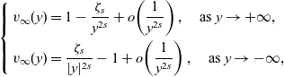 \begin{equation}\left\{\begin{array}{l} v_{\infty}(y)=1-\dfrac{\zeta_s}{y^{2s}}+o\!\left(\dfrac{1}{y^{2s}}\right),\quad \mbox{as }y\to +\infty,\\[9pt]v_{\infty}(y)=\dfrac{\zeta_s}{|y|^{2s}}-1+o\!\left(\dfrac{1}{y^{2s}}\right),\quad \mbox{as }y\to -\infty,\end{array}\right.\end{equation}
where $\zeta_s$
is a positive constant, depending only on s. There is an earlier result established for slightly shifted boundary conditions, cf. equation (23) of [Reference Nec, Nepomnyashchy and Golovin18]. Moreover, a similar exact result for a piecewise linear kinetic function exists, cf. equations for w(x) at the end of Section 2 of [Reference Volpert, Nec and Nepomnyashchy26]. Reflecting the function
$\zeta_s$
is a positive constant, depending only on s. There is an earlier result established for slightly shifted boundary conditions, cf. equation (23) of [Reference Nec, Nepomnyashchy and Golovin18]. Moreover, a similar exact result for a piecewise linear kinetic function exists, cf. equations for w(x) at the end of Section 2 of [Reference Volpert, Nec and Nepomnyashchy26]. Reflecting the function $v_\infty(y)$
with respect to the origin point, we can derive a backward front solution to the fractional Allen–Cahn equation.
$v_\infty(y)$
with respect to the origin point, we can derive a backward front solution to the fractional Allen–Cahn equation.
The second one is a single spike. We set $w_\infty$
as the solution of the following problem:
$w_\infty$
as the solution of the following problem:
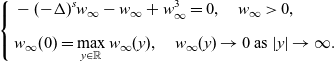 \begin{equation}\left\{\begin{aligned}&-(-\Delta)^sw_\infty-w_\infty+w_\infty^3=0,\quad w_\infty>0,\\[5pt]&w_\infty(0)=\max\limits_{y\in \mathbb{R}}w_\infty (y),\quad w_\infty(y)\to 0 \mbox{ as }|y|\to \infty.\end{aligned}\right.\end{equation}
It has been shown in [Reference Frank, Lenzmann and Silvestre8] that the solution $w_\infty$
is unique. In addition, by [Reference Frank, Lenzmann and Silvestre8, Proposition 3.1] and [Reference Nec16, lemma 3], the following result on its asymptotic behaviour holds:
$w_\infty$
is unique. In addition, by [Reference Frank, Lenzmann and Silvestre8, Proposition 3.1] and [Reference Nec16, lemma 3], the following result on its asymptotic behaviour holds:
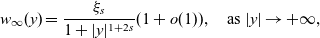 \begin{equation}w_\infty(y)=\frac{\xi_s}{1+|y|^{1+2s}}(1+o(1)),\quad \mbox{as }|y|\to +\infty,\end{equation}
where $\xi_s$
is a positive constant, depending only on s.
$\xi_s$
is a positive constant, depending only on s.
2.2 Stability analysis
In this subsection, we study some preliminary properties of the linearised eigenvalue problem. We show that the eigenvalues must be real. Moreover, we reduce the system of eigenvalue problems to a single eigenvalue problem. To study the linear stability of (1.2), we perturb (A(x), B(x)) as follows:
 \begin{equation}A_\epsilon(x,t)=A(x)+\epsilon \phi(x)e^{\lambda_{L,s}t},\quad B_\epsilon(x,t)=B(x)+\epsilon \psi(x)e^{\lambda_{L,s}t},\end{equation}
where $\lambda_{L,s}\in\mathbb{C}$
, the set of complex numbers.
$\lambda_{L,s}\in\mathbb{C}$
, the set of complex numbers.
Since we have assumed that (1.2) is invariant under the transformation $x\to -x$
and
$x\to -x$
and $x\to x+L$
, we may suppose the perturbation
$x\to x+L$
, we may suppose the perturbation $(\phi(x),\psi(x))$
has the same symmetry, and so we may assume that
$(\phi(x),\psi(x))$
has the same symmetry, and so we may assume that
 \begin{equation*} \phi,\;\ \psi\in \mathcal{X}_L,\end{equation*}
where
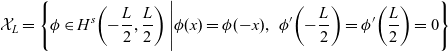 \begin{equation*} \mathcal{X}_L=\left\{\phi\in H^{s}\!\left(-\frac{L}{2},\frac{L}{2}\right)\Bigg|\phi(x)=\phi(-x),\;\ \phi'\!\left(-\frac{L}{2}\right)=\phi'\!\left(\frac{L}{2}\right)=0\right\}\end{equation*}
and $H^{s}\left(-\frac{L}{2},\frac{L}{2}\right)$
denotes the usual Sobolev space.
$H^{s}\left(-\frac{L}{2},\frac{L}{2}\right)$
denotes the usual Sobolev space.
Substituting (2.10) into (1.2) and considering the leading order part, we obtain the following eigenvalue problem:
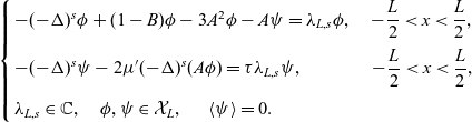 \begin{align} \left\{ \begin{array}{l} -(-\Delta)^s\phi+(1-B)\phi-3A^2\phi-A\psi=\lambda_{L,s}\phi,\quad -\dfrac{L}{2}<x<\dfrac{L}{2}, \\[9pt] -(-\Delta)^s \psi-2\mu{'}(-\Delta)^s(A\phi)=\tau\lambda_{L,s}\psi,\qquad\qquad \kern-0.8pt\!-\dfrac{L}{2}<x<\dfrac{L}{2}, \\[9pt] \lambda_{L,s}\in \mathbb{C},\quad \phi,\psi\in\mathcal{X}_L,\;\quad\;\langle\psi\rangle=0. \end{array} \right. \end{align}
We shall prove that the single (small)-spike solution $(A^-,B^-)$
of Type II is stable for all
$(A^-,B^-)$
of Type II is stable for all $\tau>0$
and all the other solutions of Type I, II or III are unstable for all
$\tau>0$
and all the other solutions of Type I, II or III are unstable for all $\tau>0$
.
$\tau>0$
.
Let
 \begin{equation}\psi=-2\mu{'}A\phi+2\mu{'}\langle A\phi \rangle+\tau\lambda_{L,s}\hat{\psi},\end{equation}
where
 \begin{equation*}\langle\hat{\psi}\rangle=0.\end{equation*}
Equation (2.12) together with (2.11) implies
 \begin{equation}-(-\Delta)^s \hat{\psi}-\tau\lambda_{L,s}\hat{\psi}=-2\mu{'}A\phi+2\mu{'}\langle A\phi \rangle.\end{equation}
Substituting (2.2) and (2.12) into (2.11), we obtain that
 \begin{equation}-(-\Delta)^s\phi-a\phi+3bA^2\phi-2\mu{'}\langle A\phi \rangle A-\tau\lambda_{L,s}A\hat{\psi}=\lambda_{L,s}\phi, \quad -\frac{L}{2}<x<\frac{L}{2},\end{equation}
where a and b are given by (2.4). If $\tau=0$
, then (2.14) becomes
$\tau=0$
, then (2.14) becomes
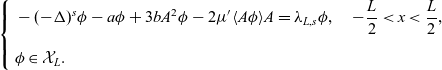 \begin{equation}\left\{\begin{aligned}&-(-\Delta)^s\phi-a\phi+3bA^2\phi-2\mu{'}\langle A\phi \rangle A=\lambda_{L,s}\phi, \quad -\frac{L}{2}<x<\frac{L}{2},\\[5pt]&\phi\in\mathcal{X}_L.\end{aligned}\right.\end{equation}
Our main result in this section is the following reduction lemma. It will be proved by variational techniques.
Lemma 2.1. Concerning the system of eigenvalue problems (2.11), we have
Lemma 2.1 implies that the stability of (2.11) is equivalent to the stability of (2.15).
Proof of Lemma 2.1. We shall prove the lemma point by point.
(a). Multiplying (2.14) by $\bar{\phi}$
, the conjugate function of
$\bar{\phi}$
, the conjugate function of $\phi$
, and integrating over I, we obtain
$\phi$
, and integrating over I, we obtain
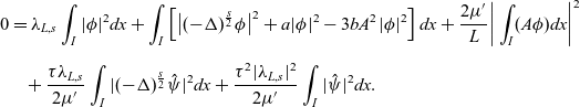
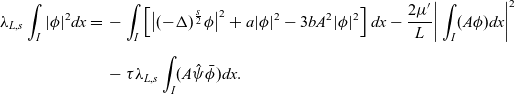 \begin{equation}\begin{aligned}\lambda_{L,s}\int_{I}|\phi|^2dx=\;&-\int_{I}\left[\big|(-\Delta)^{\frac{s}{2}}\phi\big|^2+a|\phi|^2-3bA^2|\phi|^2\right]dx-\frac{2\mu{'}}{L}\bigg|\int_{I}(A\phi) dx\bigg|^2\\[5pt]&-\tau\lambda_{L,s}\int_{I}(A\hat{\psi}\bar{\phi})dx.\end{aligned}\end{equation}
Here, we have used the expansion of $\phi$
with respect to the eigen pairs of
$\phi$
with respect to the eigen pairs of $-\Delta$
(subject to the periodic boundary condition) to treat the integration involving the fractional Laplacian. Indeed, following [Reference Cabré and Tan2], we see that the k-th eigen function of
$-\Delta$
(subject to the periodic boundary condition) to treat the integration involving the fractional Laplacian. Indeed, following [Reference Cabré and Tan2], we see that the k-th eigen function of $-\Delta$
satisfies the equation below:
$-\Delta$
satisfies the equation below:
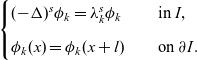 \begin{equation*} \begin{cases} (-\Delta)^s\phi_k=\lambda_k^s\phi_k \quad &\text{in } I,\\[5pt] \phi_k(x)=\phi_k(x+l)\quad &\text{on } \partial I. \end{cases} \end{equation*}
Since $(-\Delta)^s$
is a self-adjoint operator,
$(-\Delta)^s$
is a self-adjoint operator, $\lambda_k^s$
is a real number. Then, we have
$\lambda_k^s$
is a real number. Then, we have
 \begin{equation*} \begin{aligned} \int_I {\phi}_k(-\Delta)^s\phi_k dx=\int_I {\phi}_k \lambda_k^s \phi_k dx=\int_I\lambda_k^s |\phi_k|^2dx =\int_I |\lambda_k^{s/2}\phi_k|^2dx=\int_I \left|(-\Delta)^{s/2}\phi_k\right|^2dx. \end{aligned} \end{equation*}
As a consequence, we can easily get that
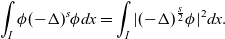 \begin{equation*}\int_{I}\phi(-\Delta)^s\phi dx=\int_{I}|(-\Delta)^{\frac s2}\phi|^2dx.\end{equation*}
Multiplying the conjugate of (2.13) by $\hat{\psi}$
and integrating over I, we get
$\hat{\psi}$
and integrating over I, we get
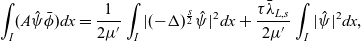 \begin{equation}\int_{I}(A\hat{\psi}\bar{\phi})dx=\frac{1}{2\mu{'}}\int_{I}|(-\Delta)^{\frac{s}{2}}\hat{\psi}|^2dx+\frac{\tau\bar{\lambda}_{L,s}}{2\mu{'}}\int_{I}|\hat{\psi}|^2dx,\end{equation}
where we have used $\langle\psi\rangle=0$
. Substituting (2.17) into (2.16) gives
$\langle\psi\rangle=0$
. Substituting (2.17) into (2.16) gives
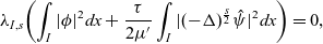
 \begin{align}\begin{split}0=\;&\lambda_{L,s}\int_{I}|\phi|^2dx+\int_{I}\left[\big|(-\Delta)^{\frac{s}{2}}\phi\big|^2+a|\phi|^2-3bA^2|\phi|^2\right]dx+\frac{2\mu{'}}{L}\bigg|\int_{I}(A\phi) dx\bigg|^2\\[5pt]&\!\!+\frac{\tau\lambda_{L,s}}{2\mu{'}}\int_{I}|(-\Delta)^{\frac{s}{2}}\hat{\psi}|^2dx+\frac{\tau^2|\lambda_{L,s}|^2}{2\mu{'}}\int_{I}|\hat{\psi}|^2dx.\end{split}\end{align}
Taking the imaginary part of (2.18), we obtain
 \begin{equation}\lambda_{I,s}\!\left(\int_{I}|\phi|^2dx+\frac{\tau}{2\mu{'}}\int_I|(-\Delta)^{\frac{s}{2}}\hat{\psi}|^2dx\right)=0,\end{equation}
where $\lambda_{L,s}=\lambda_{R,s}+\sqrt{-1}\lambda_{I,s}$
. As a consequence of (2.19), we get that
$\lambda_{L,s}=\lambda_{R,s}+\sqrt{-1}\lambda_{I,s}$
. As a consequence of (2.19), we get that
 \begin{equation*}\lambda_{I,s}=0.\end{equation*}
Therefore, $\lambda_{L,s}$
is real.
$\lambda_{L,s}$
is real.
(b). We introduce two quadratic forms, as follows:
 \begin{equation}L[\phi] := \int_{I}\left[\big|(-\Delta)^{\frac{s}{2}}\phi\big|^2+a|\phi|^2-3bA^2|\phi|^2\right]dx+\frac{2\mu{'}}{L}\left(\int_{I}|A\phi| dx\right)^2,\end{equation}
and
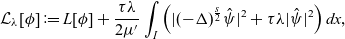 \begin{equation}\mathcal{L}_\lambda[\phi] := L[\phi]+\frac{\tau\lambda}{2\mu{'}}\int_{I}\left(|(-\Delta)^{\frac{s}{2}}\hat{\psi}|^2+\tau\lambda|\hat{\psi}|^2\right)dx,\end{equation}
observing that for $\tau\geq 0$
and
$\tau\geq 0$
and $\lambda\geq 0$
 \begin{equation}\mathcal{L}_0[\phi]=L[\phi],\quad L[\phi]\leq \mathcal{L}_\lambda[\phi].\end{equation}
Note that if all eigenvalues of (2.15) are negative, then the quadratic form $L[\phi]$
is positive definite, which together with (2.22) implies that
$L[\phi]$
is positive definite, which together with (2.22) implies that $\mathcal{L}_\lambda[\phi]$
is positive definite if
$\mathcal{L}_\lambda[\phi]$
is positive definite if $\lambda \geq 0$
. Now, we shall prove the second point by contradiction. Suppose
$\lambda \geq 0$
. Now, we shall prove the second point by contradiction. Suppose $\lambda_{L,s}\geq 0$
be an eigenvalue of (2.11), then by (2.18) we obtain that
$\lambda_{L,s}\geq 0$
be an eigenvalue of (2.11), then by (2.18) we obtain that
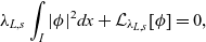 \begin{equation*}\lambda_{L,s}\int_{I}|\phi|^2dx+\mathcal{L}_{\lambda_{L,s}}[\phi]=0,\end{equation*}
which is clearly impossible. Thus, we have shown that all eigenvalues of (2.11) must be negative.
(c). Suppose (2.15) has a positive eigenvalue. Then,
 \begin{equation*}-\mu_{L,e}=\min\limits_{\phi\in \mathcal{X}_L,\int_I\phi^2dx=1}L[\phi].\end{equation*}
has a positive value $\mu_{L,e}>0$
. We claim that (2.11) admits a positive eigenvalue. Fix
$\mu_{L,e}>0$
. We claim that (2.11) admits a positive eigenvalue. Fix $\lambda\in[0,+\infty)$
, we consider another eigenvalue problem:
$\lambda\in[0,+\infty)$
, we consider another eigenvalue problem:
 \begin{equation}-\!\mu(\lambda)=\min\limits_{\phi\in \mathcal{X}_L,\int_I\phi^2dx=1}\mathcal{L}_\lambda[\phi].\end{equation}
In addition, since the operator $(-(-\Delta)^s-\tau\lambda_{L,s})$
is invertible, by (2.13) we can obtain
$(-(-\Delta)^s-\tau\lambda_{L,s})$
is invertible, by (2.13) we can obtain
 \begin{equation}\hat{\psi}=(-(-\Delta)^s-\tau\lambda_{L,s})^{-1}(-2\mu{'}A\phi+2\mu{'}\langle A\phi \rangle).\end{equation}
Substituting (2.24) into (2.21), then $\mathcal{L}_\lambda[\phi]$
depends only on
$\mathcal{L}_\lambda[\phi]$
depends only on $\phi$
, and we can regard it as an energy functional of
$\phi$
, and we can regard it as an energy functional of $\phi$
. Hence, a minimiser
$\phi$
. Hence, a minimiser $\phi$
of (2.23) satisfies the equation:
$\phi$
of (2.23) satisfies the equation:
 \begin{equation}-(-\Delta)^s\phi-a\phi+3bA^2\phi-2\mu{'}\langle A\phi \rangle A-\tau\lambda A\hat{\psi}=\mu(\lambda)\phi,\quad \phi\in\mathcal{X}_L,\end{equation}
where $\hat{\psi}\in \mathcal{X}_L$
is given by (2.13). By (2.22), we have
$\hat{\psi}\in \mathcal{X}_L$
is given by (2.13). By (2.22), we have $\mu(\lambda)\leq \mu_{L,e}$
. Moreover, since
$\mu(\lambda)\leq \mu_{L,e}$
. Moreover, since $\hat{\psi}$
is continuous with respect to
$\hat{\psi}$
is continuous with respect to $\lambda$
in
$\lambda$
in $[0,\infty)$
, we see that
$[0,\infty)$
, we see that $\mu(\lambda)$
is also continuous in
$\mu(\lambda)$
is also continuous in $[0,\infty)$
. Let us consider the following algebraic equation:
$[0,\infty)$
. Let us consider the following algebraic equation:
 \begin{equation*}h(\lambda) := \mu(\lambda)-\lambda=0,\quad \lambda\in [0,\infty).\end{equation*}
By assumption, $h(0)=\mu(0)=\mu_{L,e}>0$
. On the other hand, for
$h(0)=\mu(0)=\mu_{L,e}>0$
. On the other hand, for $\lambda>2\mu_{L,e}$
,
$\lambda>2\mu_{L,e}$
,
 \begin{equation*}h(\lambda)\leq \mu_{L,e}-\lambda<-\mu_{L,e}<0.\end{equation*}
By the intermediate value theorem, there exists a $\lambda_{L,s}\in (0,2\mu_{L,e})$
such that
$\lambda_{L,s}\in (0,2\mu_{L,e})$
such that $h(\lambda_{L,s})=0$
. Substituting
$h(\lambda_{L,s})=0$
. Substituting $\mu(\lambda_{L,s})=\lambda_{L,s}$
into (2.25), we see that
$\mu(\lambda_{L,s})=\lambda_{L,s}$
into (2.25), we see that $\lambda_{L,s}$
is an eigenvalue of (2.11). Thus, we have shown the part (c) of Lemma 2.1 and it finishes the whole proof.
$\lambda_{L,s}$
is an eigenvalue of (2.11). Thus, we have shown the part (c) of Lemma 2.1 and it finishes the whole proof.
3 Steady states: Proof of Theorem 1.1
In this section, we introduce three types of patterns for the solution A of (2.3) in detail.
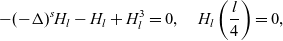
Type I (Double-front solutions). Let $\mu{'}<1$
, then
$\mu{'}<1$
, then $b<0,\, a<0$
. We rescale A as follows:
$b<0,\, a<0$
. We rescale A as follows:
 \begin{equation*}A(x)=\sqrt{\frac{a}{b}}H_{l}\left((-a)^{\frac{1}{2s}}x\right).\end{equation*}
where $l=(-a)^{\frac{1}{2s}}L$
and
$l=(-a)^{\frac{1}{2s}}L$
and $H_l$
solves
$H_l$
solves
 \begin{equation*}-(-\Delta)^sH_l+H_l-H^3_l=0,\end{equation*}
with the following boundary and symmetry conditions:
 \begin{equation*}H'_{\!\!l}\!\left(-\frac{l}{2}\right)=H'_{\!\!l}\!\left(\frac{l}{2}\right)=0,\quad H_l(y)=H_l(-y),\quad H'_{\!\!l}(y)<0 \ \mbox{ for }0<y<\frac{l}{2}.\end{equation*}
In this case, $H_l$
looks like a backward front connected to a forward front. More precisely, we need to introduce a front
$H_l$
looks like a backward front connected to a forward front. More precisely, we need to introduce a front $v_l$
in a bounded interval which satisfies the following equation:
$v_l$
in a bounded interval which satisfies the following equation:
 \begin{equation}\left\{\begin{aligned}&-(-\Delta)^sv_{l}+v_{l}-v_{l}^3=0,\quad v{'}_{\!\!l}>0,\ -\frac{l}{4}<y<\frac{l}{4},\\ &v_{l}(0)=0,\quad v{'}_{\!\!l}\!\left(-\frac{l}{4}\right)=v{'}_{\!\!l}\!\left(\frac{l}{4}\right)=0.\end{aligned}\right.\end{equation}
We remark that the existence of the forward front solution to (3.1) is ensured by [Reference Gui, Zhang and Du10, Theorem 1.2]. Then, we have
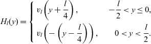 \begin{equation*}H_l(y)=\left\{\begin{aligned}&v_{l}\!\left(y+\frac{l}{4}\right),\ &-\frac{l}{2}<y\leq 0,\\ &v_{l}\!\left(-\left(y-\frac{l}{4}\right)\right),\ &0<y<\frac{l}{2}.\end{aligned}\right.\end{equation*}
The consistency condition (2.4) becomes
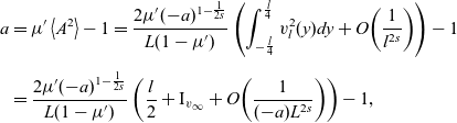 \begin{equation}\begin{aligned}a&=\mu{'}\left\langle A^2\right\rangle-1=\frac{2\mu{'}(-a)^{1-\frac{1}{2s}}}{L(1-\mu{'})}\left(\int_{-\frac{l}{4}}^{\frac{l}{4}}v_{l}^2(y)dy+O\!\left(\frac{1}{l^{2s}}\right)\right)-1\\[5pt]&=\frac{2\mu{'}(-a)^{1-\frac{1}{2s}}}{L(1-\mu{'})}\left(\frac{l}{2}+\mathrm{I}_{v_\infty}+O\!\left(\frac{1}{(-a)L^{2s}}\right)\right)-1,\end{aligned}\end{equation}
where
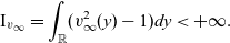 \begin{equation*}\mathrm{I}_{v_\infty}=\int_{\mathbb{R}}(v_{\infty}^2(y)-1)dy<+\infty.\end{equation*}
Therefore, if $L\gg 1$
, (3.2) can be solved if and only if the equation:
$L\gg 1$
, (3.2) can be solved if and only if the equation:
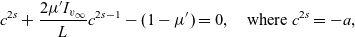 \begin{equation}c^{2s}+\frac{2\mu{'}I_{v_\infty}}{L }c^{2s-1}-(1-\mu{'})=0,\quad \mbox{where }c^{2s}=-a,\end{equation}
has a positive solution. Indeed, it is not difficult to check that
 \begin{equation*}f(x)=\frac{(1-\mu{'})-x^{2s}}{x^{2s-1}}\end{equation*}
is a strictly monotonically decreasing function for positive x. In addition, $\,f(x)\to +\infty$
as
$\,f(x)\to +\infty$
as $x\to { 0^+}$
and
$x\to { 0^+}$
and $f\!\left((1-\mu{'})^{\frac{1}{2s}}\right)=0$
, and so we can always find a unique
$f\!\left((1-\mu{'})^{\frac{1}{2s}}\right)=0$
, and so we can always find a unique $c\in\!\left(0,(1-\mu{'})^{\frac{1}{2s}}\right)$
such that
$c\in\!\left(0,(1-\mu{'})^{\frac{1}{2s}}\right)$
such that
 \begin{equation*}f(c)=\frac{2\mu{'}\mathrm{I}_{v_\infty}}{L(1-\mu{'})}.\end{equation*}
Type II (Single-spike solutions). Let $\mu{'}>1,\,A(x)>0$
. Then,
$\mu{'}>1,\,A(x)>0$
. Then, $b=\mu{'}-1>0$
and we must have
$b=\mu{'}-1>0$
and we must have $a>0$
in order to ensure that (2.3) has a solution. We rescale A as follows:
$a>0$
in order to ensure that (2.3) has a solution. We rescale A as follows:
 \begin{equation}A(x)=\sqrt{\frac{a}{b}}H_l(y),\end{equation}
where
 \begin{equation}y=a^{\frac{1}{2s}}x,\quad l=a^{\frac{1}{2s}}L.\end{equation}
Then, $H_l$
is the unique solution of the following ordinary differential equation:
$H_l$
is the unique solution of the following ordinary differential equation:
 \begin{equation*}-(-\Delta)^sH_l-H_l+H_l^3=0, \quad H_l(y)>0, \quad H_l(-y)=H_l(y),\end{equation*}
satisfying
 \begin{equation*}H'_{\!\!l}\!\left(-\frac{l}{2}\right)=H'_{\!\!l}\!\left(\frac{l}{2}\right)=0,\quad H'_{\!\!l}(y)<0 \ \mbox{ for }0<y<\frac{l}{2}.\end{equation*}
In this case, we see that for $l\gg 1$
,
$l\gg 1$
,
 \begin{equation*}H_l(y)=w_\infty(y)+O\!\left(\frac{1}{l^{1+2s}}\right),\end{equation*}
where
 \begin{equation*}w_\infty(y)=\frac{\xi_s}{1+|y|^{1+2s}}(1+o(1)).\end{equation*}
Now, we turn to check the consistency of our earlier calculation in (2.4). Substituting (3.4) into (2.4) and by simple computations, we arrive at
 \begin{equation}c^{2s}-2\beta_L^1c^{2s-1}+1=0,\end{equation}
where
 \begin{equation*}c=a^{\frac{1}{2s}},\quad \beta_L^1=\frac{\mu{'}}{2L(\mu{'}-1)}\int_{-cL/2}^{cL/2}H_{cL}^2(y)dy.\end{equation*}
Since $L\gg 1$
, we have
$L\gg 1$
, we have
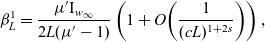 \begin{equation}\beta_L^1=\frac{\mu{'}\mathrm{I}_{w_\infty}}{2L(\mu{'}-1)}\left(1+O\!\left(\frac{1}{(cL)^{1+2s}}\right)\right),\end{equation}
where
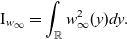 \begin{equation*}\mathrm{I}_{w_\infty}=\int_{\mathbb{R}}w_\infty^2(y)dy.\end{equation*}
Equation (3.6) has a solution if
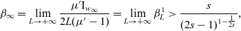 \begin{equation}\beta_\infty=\lim\limits_{L\to+\infty}\frac{\mu{'}\mathrm{I}_{w_\infty}}{2L(\mu{'}-1)}=\lim\limits_{L\to+\infty}\beta_L^1>\frac{s}{(2s-1)^{1-\frac{1}{2s}}},\end{equation}
where we have used the theory of the existence of solutions to equation (3.6):
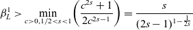 \begin{equation*}\beta_L^1>\min\limits_{c>0,1/2<s<1}\!\left(\frac{c^{2s}+1}{2c^{2s-1}}\right)=\frac{s}{(2s-1)^{1-\frac{1}{2s}}}\end{equation*}
and noted that (1.8) forces $\mu{'}\to 1$
.
$\mu{'}\to 1$
.
Under the condition (3.8), we can easily obtain that equation (3.6) has two solutions. As a consequence, we have obtained two single-spike solutions:
 \begin{equation*}A^{\pm}=\frac{(c^{\pm})^{s}}{\sqrt{\mu{'}-1}}H_{c^{\pm}L}(c^{\pm}x),\quad B^{\pm}(x)=-\mu{'}(A^\pm)^2+\mu{'}\langle(A^\pm)^2\rangle\end{equation*}
with $c^-<c^+$
. We will call
$c^-<c^+$
. We will call $(A^-,B^-)$
the single (small)-spike solution and
$(A^-,B^-)$
the single (small)-spike solution and $(A^+,B^+)$
the single (large)-spike solution. This completes the proof of Type II solutions.
$(A^+,B^+)$
the single (large)-spike solution. This completes the proof of Type II solutions.
Type III (Double-spike solutions). Assume that $\mu{'}>1$
and that A(x) changes sign. Similar to Type II solutions, we rescale A(x) as in (3.4) and set
$\mu{'}>1$
and that A(x) changes sign. Similar to Type II solutions, we rescale A(x) as in (3.4) and set $y=a^{\frac{1}{2s}}x,l=a^{\frac{1}{2s}}L$
. Then,
$y=a^{\frac{1}{2s}}x,l=a^{\frac{1}{2s}}L$
. Then, $H_l(y)$
is the solution of the following ODE:
$H_l(y)$
is the solution of the following ODE:
 \begin{equation*}-(-\Delta)^sH_l-H_l+H_l^3=0,\quad H_l\left(\frac{l}{4}\right)=0,\end{equation*}
and
 \begin{equation*}H'_{\!\!l}\!\left(-\frac{l}{2}\right)= H'_{\!\!l}\!\left(\frac{l}{2}\right)=0,\quad H_l(y)=H_l(-y),\quad H'_{\!\!l}(y)>0\;\ \mbox{ for }\;\ 0<y<\frac{l}{2}.\end{equation*}
In this case, $H_l$
looks like the superposition of two half solitons at the boundary points, both of which are positive and a negative interior soliton. Note that as
$H_l$
looks like the superposition of two half solitons at the boundary points, both of which are positive and a negative interior soliton. Note that as $l\gg 1$
, then
$l\gg 1$
, then
 \begin{equation*}H_l(y)=w_\infty\!\left(y+\frac{l}{2}\right)-w_\infty+w_\infty\!\left(y-\frac{l}{2}\right)+O\!\left(\frac{1}{l^{1+2s}}\right),\quad -\frac{l}{2}<y<\frac{l}{2}.\end{equation*}
It is easy to see that the consistency condition (2.4) implies
 \begin{equation}\begin{aligned}a=\mu{'}\langle A^2\rangle-1=\frac{\mu{'}a^{1-\frac{1}{2s}}}{L(\mu{'}-1)}\left(2\int_{-\infty}^{\infty}w_\infty^2(y)dy+O\!\left(\frac{1}{(a^{\frac{1}{2s}}L)^{1+2s}}\right)\right)-1.\end{aligned}\end{equation}
Therefore, for $L\gg 1$
, (3.9) can be solved if and only if the equation
$L\gg 1$
, (3.9) can be solved if and only if the equation
 \begin{equation*}c^{2s}-2\beta_L^2c^{2s-1}+1=0,\end{equation*}
has a solution, where
 \begin{equation*}\beta_L^2=\frac{\mu{'}\mathrm{I}_{w_\infty}}{L(\mu{'}-1)}\left(1+O\!\left(\frac{1}{(a^{1/{2s}}L)^{1+2s}}\right)\right),\end{equation*}
with
 \begin{equation*}\mathrm{I}_{w_\infty}=\int_{\mathbb{R}}w_\infty^2dy.\end{equation*}
This is the case if
 \begin{equation*}2\beta_\infty=\lim\limits_{L\to+\infty}\beta_L^2>\frac{s}{(2s-1)^{1-\frac{1}{2s}}}\end{equation*}
and it is equivalent to (1.9).
Following a similar process as we discussed for Type II solutions, we can derive two solutions $(A^\pm,B^\pm)$
. Here,
$(A^\pm,B^\pm)$
. Here, $(A^-,B^-)$
is called the double (small)-spike solution and
$(A^-,B^-)$
is called the double (small)-spike solution and $(A^+,B^+)$
is called the double (large)-spike solution. This completes the proof of existence of Type III solutions. Thus, we have solved equation (1.2) with
$(A^+,B^+)$
is called the double (large)-spike solution. This completes the proof of existence of Type III solutions. Thus, we have solved equation (1.2) with $L\gg 1$
in all three cases. As a consequence, we get Theorem 1.1.
$L\gg 1$
in all three cases. As a consequence, we get Theorem 1.1.
4 Proof of Theorem 1.2
In this section, we prove the linear stability or instability of solutions established in Theorem 1.1. In particular, we shall apply the theory of the related non-local eigenvalue problems and the variational characterisation of eigenvalues. Our approach is a generalisation of [Reference Norbury, Wei and Winter19] from the case $s=1$
to
$s=1$
to $\frac{1}{2}<s<1$
.
$\frac{1}{2}<s<1$
.
4.1 Stability of single (small)-spike solution of Type II
In this section, we prove the stability of the single (small)-spike solution of Type II. Let A(x), B(x) be the single (small)-spike solution of Type II obtained in Section 3. Then, as $L\to\infty$
, we have
$L\to\infty$
, we have
 \begin{equation*}A(x)=\sqrt{\frac{a}{\mu{'}-1}}w_\infty(cx)+O\!\left(\frac{1}{(cL)^{1+2s}}\right),\quad B(x)=-\mu{'}A^2+\mu{'}\langle A^2\rangle.\end{equation*}
Here, the constant $c=a^{\frac{1}{2s}}$
satisfies
$c=a^{\frac{1}{2s}}$
satisfies
 \begin{equation*}c^{2s}-2\beta_L^1c^{2s-1}+1=0,\quad \beta_L^1=\frac{\mu{'}\mathrm{I}_{w_\infty}}{2L(\mu{'}-1)},\quad \textrm{as} \quad L\to\infty.\end{equation*}
By Lemma 2.1, to prove the stability, we just need to consider the positive definiteness of $L[\phi]$
, defined by (2.20). By the rescaling (3.4) and (3.5), we see that
$L[\phi]$
, defined by (2.20). By the rescaling (3.4) and (3.5), we see that $L[\phi]$
can be rewritten as:
$L[\phi]$
can be rewritten as:
 \begin{equation}L[\phi]=a^{1-\frac{1}{2s}}\!\left(\int_{\tilde{I}}\left(\big|(-\Delta)^{\frac{s}{2}}\tilde{\phi}\big|^2+\big|\tilde{\phi}\big|^2-3H_l^2\tilde{\phi}^2\right)dy+\frac{2\mu{'}}{L(\mu{'}-1)a^{\frac{1}{2s}}}\left(\int_{\tilde{I}}H_l\tilde{\phi} dy\right)^2\right),\end{equation}
where $\tilde{I} := [-l/2,l/2]$
and
$\tilde{I} := [-l/2,l/2]$
and $\tilde{\phi}(y)=\phi(x)$
. Thus, as
$\tilde{\phi}(y)=\phi(x)$
. Thus, as $L\to \infty$
we obtain the following quadratic form in
$L\to \infty$
we obtain the following quadratic form in $H^1(\mathbb{R})$
:
$H^1(\mathbb{R})$
:
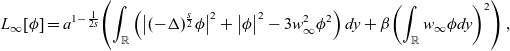 \begin{equation}L_\infty[\phi]=a^{1-\frac{1}{2s}}\!\left(\int_{\mathbb{R}}\left(\big|(-\Delta)^{\frac{s}{2}}\phi\big|^2+\big|\phi\big|^2-3w_\infty^2\phi^2\right)dy+\beta\!\left(\int_{\mathbb{R}}w_\infty\phi dy\right)^2\right),\end{equation}
where
 \begin{equation*}\phi\in\mathcal{X}_\infty:=\left\{\,f\mid f\in H^{s}(\mathbb{R}),\ f(-y)=f(y)\right\}\quad\mbox{and}\quad\beta=\lim\limits_{L\to\infty}\frac{2\mu{'}}{L(\mu{'}-1)a^{\frac{1}{2s}}}.\end{equation*}
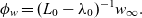
The study of (4.2) is equivalent to the study of the following non-local eigenvalue problem:
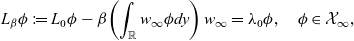 \begin{equation}L_\beta\phi := L_0\phi-\beta\!\left(\int_{\mathbb{R}}w_\infty\phi dy\right)w_\infty=\lambda_0\phi,\quad \phi\in \mathcal{X}_\infty,\end{equation}
where
 \begin{equation*}L_0\phi=-(-\Delta)^s\phi-\phi+3w_\infty^2\phi.\end{equation*}
Lemma 4.1. Concerning the linear operator $L_0$
, we have the following conclusions:
$L_0$
, we have the following conclusions:
-
(a)
$\mathrm{Ker}\{L_0\}=\left\{cw'_{\!\!\infty}(y)|c\in \mathbb{R}\right\}$
. -
(b)
$L_0$
has a unique (principal) positive eigenvalue
$\nu_1>0$
. The associated eigenfunction
$\phi_0(y)$
is positive and even after a translation if necessary. -
(c)
$L_0\!\left(\frac{1}{2}\left(w_\infty(y)+\frac{y}{s}w'_{\!\!\infty}(y)\right)\right)=w_\infty(y)$
.


Proof. We shall prove the Lemma 4.1 point by point.
(1). For the point of (a), we refer the readers to [Reference Frank, Lenzmann and Silvestre8, Theorem 3].
(2). The proof of (b) follows by the variational characterisation of the eigenvalues:
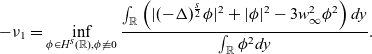 \begin{equation}-\nu_1=\inf\limits_{\phi\in H^{s}(\mathbb{R}),\phi\not\equiv 0}\frac{\int_{\mathbb{R}}\left(|(-\Delta)^{\frac{s}{2}}\phi|^2+|\phi|^2-3w_\infty^2\phi^2\right)dy}{\int_{\mathbb{R}}\phi^2dy}.\end{equation}
Let $\phi=w_\infty$
, we have
$\phi=w_\infty$
, we have
 \begin{equation*}\int_{\mathbb{R}}\left(|(-\Delta)^{\frac{s}{2}}w_\infty|^2+|w_\infty|^2-3w_\infty^4\right)dy=-2\int_{\mathbb{R}}w_\infty^4dy<0.\end{equation*}
Thus, $\nu_1>0$
. In fact,
$\nu_1>0$
. In fact, $\nu_1$
is the unique positive eigenvalue. By the variational characterisation (4.4) of
$\nu_1$
is the unique positive eigenvalue. By the variational characterisation (4.4) of $\nu_1$
, we see that the corresponding eigenfunction can be chosen to be positive. Since
$\nu_1$
, we see that the corresponding eigenfunction can be chosen to be positive. Since $w_\infty$
is even, the eigenfunction can also be chosen to be even. Indeed, suppose
$w_\infty$
is even, the eigenfunction can also be chosen to be even. Indeed, suppose $\phi$
is not even, then we write
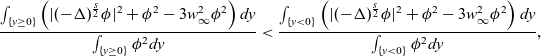
$\phi$
is not even, then we write
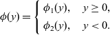 \begin{equation*}\phi(y)=\left\{\begin{aligned}&\phi_1(y),\quad y\geq 0,\\&\phi_2(y),\quad y<0.\end{aligned}\right.\end{equation*}
If
 \begin{equation}\begin{aligned}\frac{\int_{\{y\geq0\}}\left(|(-\Delta)^{\frac{s}{2}}\phi|^2+\phi^2-3w_\infty^2\phi^2\right)dy}{\int_{\{y\geq 0\}}\phi^2dy}<\frac{\int_{\{y<0\}}\left(|(-\Delta)^{\frac{s}{2}}\phi|^2+\phi^2-3w_\infty^2\phi^2\right)dy}{\int_{\{y< 0\}}\phi^2dy},\end{aligned}\end{equation}
we may choose
 \begin{equation*}\phi_{e}(y)=\left\{\begin{aligned}&\phi_1(y),\ y\geq 0,\\&\phi_1(-y),\ y<0.\end{aligned}\right.\end{equation*}
Then,
 \begin{equation*}\begin{aligned}\frac{\int_{\mathbb{R}}\left(|(-\Delta)^{\frac{s}{2}}\phi_{e}|^2+\phi_{e}^2-3w_\infty^2\phi_{e}^2\right)dy}{\int_{\mathbb{R}}\phi_{e}^2dy}<\frac{\int_{\mathbb{R}}\left(|(-\Delta)^{\frac{s}{2}}\phi|^2+\phi^2-3w_\infty^2\phi^2\right)dy}{\int_{\mathbb{R}}\phi^2dy},\end{aligned}\end{equation*}
and thus the function $\phi$
is not the eigenfunction of the principal eigenvalue. This is a contradiction. Similarly, we arrive at a contradiction if the reverse inequality of (4.5) holds. If we have equality in (4.5), then we can construct an even eigenfunction
$\phi$
is not the eigenfunction of the principal eigenvalue. This is a contradiction. Similarly, we arrive at a contradiction if the reverse inequality of (4.5) holds. If we have equality in (4.5), then we can construct an even eigenfunction $\phi_{e}$
from the eigenfunction
$\phi_{e}$
from the eigenfunction $\phi$
in the same way as above with the same eigenvalue. Since the principal eigenfunction is unique and an even eigenfunction exists, the eigenfunction has to be even.
$\phi$
in the same way as above with the same eigenvalue. Since the principal eigenfunction is unique and an even eigenfunction exists, the eigenfunction has to be even.
(3). By simple computations, we have
 \begin{equation*}L_0w_\infty=2w_\infty^3.\end{equation*}
On the other hand, setting $w_\lambda(y)=w_\infty(\lambda y)$
, we have
$w_\lambda(y)=w_\infty(\lambda y)$
, we have
 \begin{equation*}\begin{aligned}-(-\Delta)^sw_\lambda(y)=-\lambda^{2s}(-\Delta)^sw_\infty(\lambda y)=\lambda^{2s}(w_\infty(\lambda y)-w_\infty^3(\lambda y)).\end{aligned}\end{equation*}
Then
 \begin{equation*}-(-\Delta)^sw_\infty(\lambda y)-w_\infty(\lambda y)+w^3_\infty(\lambda y)=(\lambda^{2s}-1)(w_\infty(\lambda y)-w_\infty^3(\lambda y)).\end{equation*}
Differenting the above equality at $\lambda=1$
gives
$\lambda=1$
gives
 \begin{equation*}-(-\Delta)^s(yw'_{\!\!\infty})-yw'_{\!\!\infty}+3w_\infty^2(yw'_{\!\!\infty})=2s(w_\infty-w_\infty^3),\end{equation*}
which implies
 \begin{equation*}L_0\!\left(\frac{1}{s}yw'_{\!\!\infty}\right)=2(w_\infty-w_\infty^3).\end{equation*}
Hence,
 \begin{equation*}L_0\!\left(\frac{1}{2}\left(w_\infty+\frac{1}{s}yw'_{\!\!\infty}\right)\right)=w_\infty,\quad L_0^{-1}w_\infty=\frac{1}{2}\left(w_\infty+\frac{1}{s}yw'_{\!\!\infty}\right).\end{equation*}
Next, we study $L_\beta$
. Since
$L_\beta$
. Since $L_\beta$
is a self-adjoint operator, the eigenvalues of
$L_\beta$
is a self-adjoint operator, the eigenvalues of $L_\beta$
must be real.
$L_\beta$
must be real.
Theorem 4.1. Let $L_\beta$
be defined in (4.3). Then
$L_\beta$
be defined in (4.3). Then
-
(a) The eigenvalue problem (4.3) has an eigenfunction
$\phi\in\mathcal{X}_\infty$
with positive eigenvalue if and only if
$\beta<\frac{4s}{(2s-1)\mathrm{I}_{w_\infty}}$
. Moreover, for
$0<\beta<\frac{4s}{(2s-1)\mathrm{I}_{w_\infty}}$
, this positive eigenvalue is simple and isolated. -
(b) If
$\beta=\frac{4s}{(2s-1)\mathrm{I}_{w_\infty}}$
, then the eigenvalue problem (4.3) has a zero eigenvalue with eigenfunction
$\phi_0=w_\infty+\frac{1}{s}yw'_\infty(y)$
. -
(c) If
$\beta>\frac{4s}{(2s-1)\mathrm{I}_{w_\infty}}$
, then there exists
$C>0$
such that (4.6)
\begin{equation}\int_{\mathbb{R}}\left(\big|(-\Delta)^{\frac{s}{2}}\phi\big|^2+\big|\phi\big|^2-3w_\infty^2\phi^2\right)dy+\beta\!\left(\int_{\mathbb{R}}w_\infty\phi dy\right)^2\geq C\int_{\mathbb{R}}\phi^2dy.\end{equation}


Proof. We shall divide the proof into three parts.
(1). By Lemma 4.1, $\nu_1$
is the only positive eigenvalue of
$\nu_1$
is the only positive eigenvalue of $L_0$
and the corresponding eigenfunction
$L_0$
and the corresponding eigenfunction $\phi_0$
is positive and belongs to
$\phi_0$
is positive and belongs to $\mathcal{X}_\infty$
. For fixed
$\mathcal{X}_\infty$
. For fixed $\lambda_0>0, \lambda_0\neq \nu_1, (L_0-\lambda_0)^{-1}$
exists in
$\lambda_0>0, \lambda_0\neq \nu_1, (L_0-\lambda_0)^{-1}$
exists in $\mathcal{X}_\infty$
. For
$\mathcal{X}_\infty$
. For $\beta>0$
and
$\beta>0$
and $\lambda_0>0$
, we may rewrite (4.3) as:
$\lambda_0>0$
, we may rewrite (4.3) as:
 \begin{equation}\phi=\beta\!\left(\int_{\mathbb{R}}w_\infty \phi dy\right)\left((L_0-\lambda_0)^{-1}w_\infty\right).\end{equation}
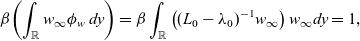
Assume first that (4.7) holds. Multiplying (4.7) by $w_\infty$
and integrating over
$w_\infty$
and integrating over $\mathbb{R}$
gives
$\mathbb{R}$
gives
 \begin{equation}\int_{\mathbb{R}}w_\infty\phi dy=\beta\!\left(\int_{\mathbb{R}}w_\infty \phi dy\right)\int_{\mathbb{R}}\left((L_0-\lambda_0)^{-1}w_\infty\right)w_\infty dy.\end{equation}
Now we claim that
 \begin{equation*}\int_{\mathbb{R}}w_\infty\phi\ dy \neq 0.\end{equation*}
We prove the conclusion by contradiction. Suppose that
 \begin{equation*}\int_{\mathbb{R}}w_\infty\phi dy = 0.\end{equation*}
Then, (4.3) implies that
 \begin{equation*}L_0\phi=\lambda_0\phi,\quad \lambda_0>0,\quad \phi\in \mathcal{X}_\infty.\end{equation*}
Using Lemma 4.1, we know that $\phi$
is positive, it follows that
$\phi$
is positive, it follows that
 \begin{equation*}\int_{\mathbb{R}}w_\infty\phi\ dy\neq 0.\end{equation*}
This is a contradiction. Therefore, (4.8) implies
 \begin{equation}\rho(\lambda_0) := \beta\int_{\mathbb{R}}\left((L_0-\lambda_0)^{-1}w_\infty\right)w_\infty dy-1=0,\quad \lambda_0>0.\end{equation}
On the other hand, suppose that (4.9) holds. For the positive root $\lambda_0$
of (4.9), we set
$\lambda_0$
of (4.9), we set
 \begin{equation*}\phi_w=(L_0-\lambda_0)^{-1}w_\infty.\end{equation*}
By (4.9), we have
 \begin{equation*}\beta\!\left(\int_{\mathbb{R}}w_\infty \phi_w\ dy\right) =\beta\int_{\mathbb{R}}\left((L_0-\lambda_0)^{-1}w_\infty\right)w_\infty dy=1,\end{equation*}
and therefore $\lambda_0\neq 0$
and
$\lambda_0\neq 0$
and $\phi_w>0$
solve (4.7). Thus, for
$\phi_w>0$
solve (4.7). Thus, for $\beta>0$
problem (4.3) has a positive eigenvalue if and only if the algebraic equation (4.9) has a positive root. We now discuss (4.9). It is not difficult to check that
$\beta>0$
problem (4.3) has a positive eigenvalue if and only if the algebraic equation (4.9) has a positive root. We now discuss (4.9). It is not difficult to check that $\rho(\lambda)<0$
for
$\rho(\lambda)<0$
for $\lambda>\nu_1$
. Thus, we only need to consider
$\lambda>\nu_1$
. Thus, we only need to consider $\lambda\in (0,\nu_1)$
. In this case,
$\lambda\in (0,\nu_1)$
. In this case,
 \begin{equation*}\rho'(\lambda)=\beta\int_{\mathbb{R}}\left(w_\infty(L_0-\lambda)^{-2}w_\infty\right)dy=\beta\int_{\mathbb{R}}\left((L_0-\lambda)^{-1}w_\infty\right)^2dy>0.\end{equation*}
On the other hand, as $\lambda\to \nu_1^-, \rho(\lambda)\to\infty$
. Thus, (4.9) has a positive real root if and only if
$\lambda\to \nu_1^-, \rho(\lambda)\to\infty$
. Thus, (4.9) has a positive real root if and only if $\rho(0)<0$
. Now, we compute
$\rho(0)<0$
. Now, we compute $\rho(0)$
. By part (c) of Lemma 4.1, we have
$\rho(0)$
. By part (c) of Lemma 4.1, we have
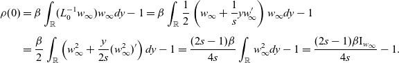 \begin{equation*}\begin{aligned}\rho(0)&=\beta\int_{\mathbb{R}}(L_0^{-1}w_\infty)w_\infty dy-1=\beta\int_{\mathbb{R}}\frac{1}{2}\left(w_\infty+\frac{1}{s}yw'_{\!\!\infty}\right)w_\infty dy-1\\[5pt]&=\frac{\beta}{2}\int_{\mathbb{R}}\left(w_\infty^2 +\frac{y}{2s}(w_\infty^2)'\right)dy-1=\frac{(2s-1)\beta}{4s}\int_{\mathbb{R}}w_\infty^2dy-1=\frac{(2s-1)\beta \mathrm{I}_{w_\infty}}{4s}-1.\end{aligned}\end{equation*}
Therefore, $\rho(0)<0$
if and only if
$\rho(0)<0$
if and only if
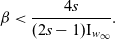 \begin{equation*}\beta<\frac{4s}{(2s-1)\mathrm{I}_{w_\infty}}.\end{equation*}
(2). Part (b) follows from part (c) of Lemma 4.1.
(3). Let
 \begin{equation*}\begin{aligned}\lambda_0=\min\limits_{\phi\in\mathcal{X}_\infty}\frac{\int_{\mathbb{R}}\left(|(-\Delta)^{\frac{s}{2}}\phi|^2+|\phi|^2-3w_\infty^2\phi^2\right)dy+\beta\left(\int_{\mathbb{R}}w_\infty\phi dy\right)^2}{\int_{\mathbb{R}}\phi^2 dy}=\min\limits_{\phi\in\mathcal{X}_\infty}\frac{\int_{\mathbb{R}}(-L_\beta\phi)\phi dy}{\int_{\mathbb{R}}\phi^2 dy}.\end{aligned}\end{equation*}
By the conclusion (a), we know that $L_\beta$
has no positive real eigenvalues since
$L_\beta$
has no positive real eigenvalues since $\beta>\frac{4s}{(2s-1)\mathrm{I}_{w_\infty}}$
. Thus,
$\beta>\frac{4s}{(2s-1)\mathrm{I}_{w_\infty}}$
. Thus, $\lambda_0\geq 0$
. We prove
$\lambda_0\geq 0$
. We prove $\lambda_0>0$
by contradiction. Suppose
$\lambda_0>0$
by contradiction. Suppose $\lambda_0=0$
, then we have a
$\lambda_0=0$
, then we have a $\phi_0\in\mathcal{X}_L$
such that
$\phi_0\in\mathcal{X}_L$
such that
 \begin{equation*}-(-\Delta)^s\phi_0-\phi_0+3w_\infty^2\phi_0-\beta\!\left(\int_{\mathbb{R}}w_\infty\phi_0 \ dy\right)w_\infty=0,\quad \int_{\mathbb{R}}\phi_0^2dy=1.\end{equation*}
Using (c) of Lemma 4.1, we see that
 \begin{equation*}-(-\Delta)^s \tilde{\phi}_0-\tilde{\phi}_0+3w_\infty^2\tilde{\phi}_0=0,\end{equation*}
where
 \begin{equation*}\tilde{\phi}_0=\phi_0-\beta\!\left(\int_{\mathbb{R}}w_\infty \phi_0 dy\right)\left(\frac{1}{2}\left(w_\infty+\frac{1}{s}yw'_{\!\!\infty}\right)\right).\end{equation*}
By (a) of Lemma 4.1, we have
 \begin{equation*}\tilde{\phi}_0=\phi_0-\beta\!\left(\int_{\mathbb{R}}w_\infty \phi_0 dy\right)\left(\frac{1}{2}\left(w_\infty+\frac{1}{s}yw'_{\!\!\infty}\right)\right)=cw'_{\!\!\infty},\end{equation*}
for some constant c.
Since $\phi_0\in\mathcal{X}_\infty$
, it follows that
$\phi_0\in\mathcal{X}_\infty$
, it follows that $\phi_0(-y)=\phi_0(y)$
. Checking the parity of both ends of the above equation, we obtain
$\phi_0(-y)=\phi_0(y)$
. Checking the parity of both ends of the above equation, we obtain $c=0$
, then
$c=0$
, then
 \begin{equation}\phi_0=\beta\!\left(\int_{\mathbb{R}}w_\infty \phi_0 dy\right)\left(\frac{1}{2}\left(w_\infty+\frac{1}{s}yw'_{\!\!\infty}\right)\right).\end{equation}
Multiplying (4.10) by $w_\infty$
and integrating over
$w_\infty$
and integrating over $\mathbb{R}$
, we have
$\mathbb{R}$
, we have
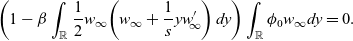 \begin{equation*}\left(1-\beta\int_{\mathbb{R}}\frac{1}{2}w_\infty\!\left(w_\infty+\frac{1}{s}yw'_{\!\!\infty}\right)dy\right)\int_{\mathbb{R}}\phi_0w_\infty dy=0.\end{equation*}
We recall that
 \begin{equation*}\int_{\mathbb{R}}\frac{1}{2}w_\infty\!\left(w_\infty+\frac{1}{s}yw'_{\!\!\infty}\right)dy=\frac{(2s-1)\mathrm{I}_{w_\infty}}{4s}.\end{equation*}
Since $\beta>\frac{4s}{(2s-1)\mathrm{I}_{w_\infty}}$
, then we have
$\beta>\frac{4s}{(2s-1)\mathrm{I}_{w_\infty}}$
, then we have $\int_{\mathbb{R}}w_\infty\phi_0\ dy=0$
and hence
$\int_{\mathbb{R}}w_\infty\phi_0\ dy=0$
and hence $\phi_0=0$
. This is a contradiction. Therefore,
$\phi_0=0$
. This is a contradiction. Therefore, $\lambda_0>0$
.
$\lambda_0>0$
.
Corollary 4.1. Let A be the single (small)-spike solution of Type II. Then there exists $c_0>0$
such that for L sufficiently large and
$c_0>0$
such that for L sufficiently large and $\phi\in\mathcal{X}_L$
, we have
$\phi\in\mathcal{X}_L$
, we have
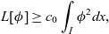 \begin{equation}L[\phi]\geq c_0\int_{I}\phi^2 dx,\end{equation}
where $L[\phi]$
is defined by (2.20).
$L[\phi]$
is defined by (2.20).
Proof. Note that
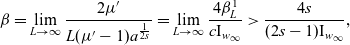 \begin{equation*}\begin{aligned}\beta =\lim\limits_{L\to\infty}\frac{2\mu{'}}{L(\mu{'}-1)a^{\frac{1}{2s}}}=\lim\limits_{L\to\infty}\frac{4\beta_L^1}{c\mathrm{I}_{w_\infty}}>\frac{4s}{(2s-1)\mathrm{I}_{w_\infty}},\end{aligned}\end{equation*}
where $\beta_L^1$
is defined in (3.7). In addition, the last inequality holds since
$\beta_L^1$
is defined in (3.7). In addition, the last inequality holds since $c<\frac{(2s-1)\beta_L^1}{s}$
and
$c<\frac{(2s-1)\beta_L^1}{s}$
and $\frac{(2s-1)\beta_L^1}{s}$
is the point such that
$\frac{(2s-1)\beta_L^1}{s}$
is the point such that $f(c)=c^{2s}-2\beta_L^1c^{2s-1}+1$
achieves its minimal value. Then, (4.11) follows from (4.6) of Theorem 4.1 and (4.1).
$f(c)=c^{2s}-2\beta_L^1c^{2s-1}+1$
achieves its minimal value. Then, (4.11) follows from (4.6) of Theorem 4.1 and (4.1).
From Lemma 2.1 and Corollary 4.1, we see that for L sufficiently large, the single (small)-spike solution of Type II is linearly stable for any $\tau>0$
.
$\tau>0$
.
4.2 Instability of other solutions
In this subsection, we will show that the other solutions are linearly unstable. By the Lemma 2.1, we just need to consider problem (2.15). To show instability, all we need to show is that the following minimisation problem admits a negative value for a certain test function:
 \begin{equation}-\mu_{L,e}=\min\limits_{\phi\in\mathcal{X}_L,\;\int_{I}\phi^2dx=1}\left[\int_{I}\left(|(-\Delta)^{\frac{s}{2}}\phi|^2+a\phi^2-3bA^2\phi^2\right)dx+\frac{2\mu{'}}{L}\left(\int_{I}A\phi dx\right)^2\right]<0,\end{equation}
which is equivalent to
 \begin{equation}-\mu_{L,e}=\min\limits_{\phi\in H^{s}(I),\;\int_{I}\phi^2dx=1}\left[\int_{I}\left(|(-\Delta)^{\frac{s}{2}}\phi|^2+a\phi^2-3bA^2\phi^2\right)dx+\frac{2\mu{'}}{L}\left(\int_{I}A\phi dx\right)^2\right]<0.\end{equation}
Thus, it is enough to find a $\phi\in H^s(I)$
such that
$\phi\in H^s(I)$
such that
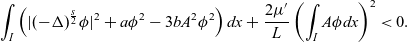 \begin{equation*}\int_{I}\left(|(-\Delta)^{\frac{s}{2}}\phi|^2+a\phi^2-3bA^2\phi^2\right)dx+\frac{2\mu{'}}{L}\left(\int_{I}A\phi dx\right)^2<0.\end{equation*}
We now consider the three types of solutions separately, with $L\gg 1$
.
$L\gg 1$
.
1. Double-front solutions of Type I. First of all, we consider the double-front solution and show that it is unstable. In this case, we choose our function such that
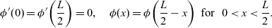 \begin{equation}\phi'(0)=\phi'\!\left(\frac{L}{2}\right)=0,\quad \phi(x)=\phi\!\left(\frac{L}{2}-x\right)\ \mbox{for }\;\ 0<x<\frac{L}{2}.\end{equation}
The last equality implies that $\phi\!\left(x+\frac{L}{4}\right)$
is an even function in
$\phi\!\left(x+\frac{L}{4}\right)$
is an even function in $\left[-\frac{L}{4},\frac{L}{4}\right]$
, and so we can extend
$\left[-\frac{L}{4},\frac{L}{4}\right]$
, and so we can extend $\phi(x)$
evenly to
$\phi(x)$
evenly to $[-L/2,0]$
. In this case,
$[-L/2,0]$
. In this case,
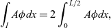 \begin{equation*}\int_{I}A\phi dx=2\int_{0}^{L/2}A\phi dx,\end{equation*}
and
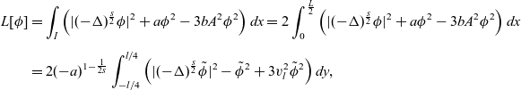 \begin{equation*}\begin{aligned}L[\phi]&=\int_{I}\left(|(-\Delta)^{\frac{s}{2}}\phi|^2+a\phi^2-3bA^2\phi^2\right)dx=2\int_{0}^{\frac{L}{2}}\left(|(-\Delta)^{\frac{s}{2}}\phi|^2+a\phi^2-3bA^2\phi^2\right)dx\\[5pt]&=2(-a)^{1-\frac{1}{2s}}\int_{-l/4}^{l/4}\left(|(-\Delta)^{\frac{s}{2}}\tilde{\phi}|^2-\tilde{\phi}^2+3v_{l}^2\tilde{\phi}^2\right)dy,\end{aligned}\end{equation*}
where $v_{l}$
is defined by (3.1) and
$v_{l}$
is defined by (3.1) and
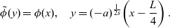 \begin{equation}\tilde{\phi}(y)=\phi(x), \quad y=(-a)^{\frac{1}{2s}}\!\left(x-\frac{L}{4}\right).\end{equation}
Let $\varphi_l$
be such that
$\varphi_l$
be such that
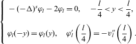 \begin{equation*}\left\{\begin{aligned}&-(-\Delta)^s\varphi_l-2\varphi_l=0,\quad -\frac{l}{4}<y<\frac{l}{4},\\[5pt]&\varphi_l(-y)=\varphi_l(y),\quad \varphi{'}_{\!\!l}\left(\frac{l}{4}\right)=-v{''}_{\!\!\!l}\left(\frac{l}{4}\right).\end{aligned}\right.\end{equation*}
In fact, $v{''}_{\!\!\!l}\left(\frac{l}{4}\right)<0$
, which we shall prove in Lemma 4.2 below.
$v{''}_{\!\!\!l}\left(\frac{l}{4}\right)<0$
, which we shall prove in Lemma 4.2 below.
Set
 \begin{equation*}\tilde{\phi}(y)=v{'}_{\!\!l}(y)+\varphi_l(y).\end{equation*}
It is easy to check that $\phi(x)$
, defined by (4.15), satisfies (4.14). We compute
$\phi(x)$
, defined by (4.15), satisfies (4.14). We compute
 \begin{equation*}\begin{aligned}-(-\Delta)^s\tilde{\phi}+\tilde{\phi}-3v_{l}^2\tilde{\phi}=-(-\Delta)^sv{'}_{\!\!l}+v{'}_{\!\!l}-3v_{l}^2v{'}_{\!\!l}-(-\Delta)^s\varphi_l+\varphi_l-3v_{l}^2\varphi_l=3(1-v_{l}^2)\varphi_l.\end{aligned}\end{equation*}
Then,
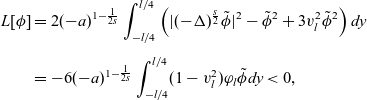 \begin{equation*}\begin{aligned}L[\phi]&=2(-a)^{1-\frac{1}{2s}}\int_{-l/4}^{l/4}\left(|(-\Delta)^{\frac{s}{2}}\tilde{\phi}|^2-\tilde{\phi}^2+3v_{l}^2\tilde{\phi}^2\right)dy\\[5pt]&=-6(-a)^{1-\frac{1}{2s}}\int_{-l/4}^{l/4}(1-v_{l}^2)\varphi_l\tilde{\phi}dy<0,\end{aligned}\end{equation*}
since
 \begin{equation*}1-v_{l}^2>0,\ \varphi_l>0,\ \tilde{\phi}>0.\end{equation*}
By (4.12), this shows that the double-front solution is unstable.
Lemma 4.2. Let $v_l$
be defined in (3.1). Then,
$v_l$
be defined in (3.1). Then, $v{''}_{\!\!\!l}\left(\frac{l}{4}\right)<0$
.
$v{''}_{\!\!\!l}\left(\frac{l}{4}\right)<0$
.
Proof. By standard elliptic regularity theory, we can show that $v_l$
is smooth enough. We set
$v_l$
is smooth enough. We set
 \begin{equation*}\psi(x)=v{'}_{\!\!l}\!\left(x+\frac{l}{4}\right).\end{equation*}
Then, it is easy to verify that
 \begin{equation}(-\Delta)^s\psi+(3w_l^2(x)-1)\psi=0, \quad \psi(x)=-\psi(-x),\quad x\in\mathbb{R},\end{equation}
where $w_l=v_l\!\left(x+\frac{l}{4}\right)$
. With the above setting, it suffices to show that
$w_l=v_l\!\left(x+\frac{l}{4}\right)$
. With the above setting, it suffices to show that $\psi'(0)<0$
. We shall prove it by contradiction. Suppose that
$\psi'(0)<0$
. We shall prove it by contradiction. Suppose that $\psi'(0)=0$
, combining with the fact that
$\psi'(0)=0$
, combining with the fact that $x=l/4$
is a local maximal point of
$x=l/4$
is a local maximal point of $v_l$
, we conclude
$v_l$
, we conclude $\psi''(0)=0$
.
$\psi''(0)=0$
.
Using the definition of the fractional Laplacian and the fact that $\psi$
is an odd function, we derive that
$\psi$
is an odd function, we derive that
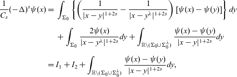 \begin{equation}\begin{aligned}\frac{1}{C_{s}}(-\Delta)^s\psi(x)=\;&\int_{\Sigma_0}\left\{\left(\frac{1}{|x-y|^{1+2s}}-\frac{1}{|x-y^\lambda|^{1+2s}}\right)\left[\psi(x)-\psi(y)\right]\right\}dy\\[5pt]&+\int_{\Sigma_0}\frac{2\psi(x)}{|x-y^\lambda|^{1+2s}}dy+\int_{\mathbb{R}\setminus(\Sigma_0\cup\Sigma_0^\lambda)}\frac{\psi(x)-\psi(y)}{|x-y|^{1+2s}}dy\\[5pt]=\;&I_1+I_2+\int_{\mathbb{R}\setminus(\Sigma_0\cup\Sigma_0^\lambda)}\frac{\psi(x)-\psi(y)}{|x-y|^{1+2s}}dy,\end{aligned}\end{equation}
where
 \begin{equation*}\Sigma_0=\left\{y\in \mathbb{R},-\frac{l}{2}<y<0\right\}\quad\mbox{and}\quad \Sigma_0^\lambda=\left\{y\in \mathbb{R},0<y<\frac{l}{2}\right\}.\end{equation*}
In the following, we shall denote $y^\lambda$
as the opposite point of y, i.e.
$y^\lambda$
as the opposite point of y, i.e. $y^\lambda=-y$
.
$y^\lambda=-y$
.
Let $x=-\delta$
and we divide
$x=-\delta$
and we divide $\Sigma_0$
into the following subregions:
$\Sigma_0$
into the following subregions:
 \begin{equation*}\Sigma_0=B_\eta\cup\Omega_{R,\eta}\cup D\cup E,\end{equation*}
where
 \begin{equation*}\begin{aligned}&B_\eta=\{-\eta\leq y\leq -2\delta\},\quad D=\{-R_c\leq y \leq -R_c+1\},\\[5pt]&\Omega_{R,\eta}=\{-R\leq y\leq -\eta\}\setminus D,\quad E=\Sigma_0\setminus(D\cup\Omega_{R,\eta}\cup \ B_\eta),\end{aligned}\end{equation*}
with $R_c\in(\eta+2,R)$
is chosen such that
$R_c\in(\eta+2,R)$
is chosen such that $\psi$
has strictly positive lower bound in D. For sufficiently small
$\psi$
has strictly positive lower bound in D. For sufficiently small $\delta$
and
$\delta$
and $\eta$
, we shall estimate
$\eta$
, we shall estimate $I_1$
in the above regions successively as follows:
$I_1$
in the above regions successively as follows:
(i). For $y\in D$
,
$y\in D$
, $\psi(y)$
is bounded away from 0 and
$\psi(y)$
is bounded away from 0 and $\psi(x)$
is sufficiently small, and so there exists a constant
$\psi(x)$
is sufficiently small, and so there exists a constant $C>0$
independent of
$C>0$
independent of $\delta$
such that
$\delta$
such that
 \begin{equation*}\psi(x)-\psi(y)<-C.\end{equation*}
Applying the Mean Value Theorem, we obtain
 \begin{equation*}\begin{aligned}\frac{1}{|x-y|^{1+2s}}-\frac{1}{|x-y^\lambda|^{1+2s}}= \frac{1}{|-x+y|^{1+2s}}-\frac{1}{|x+y|^{1+2s}}=\frac{2(1+2s)|x|}{\xi^{2+2s}}=\frac{2(1+2s)\delta}{\xi^{2+2s}},\end{aligned}\end{equation*}
where $\xi\in(|x-y|,|x-y^\lambda|)$
. Then, we have
$\xi\in(|x-y|,|x-y^\lambda|)$
. Then, we have
 \begin{equation}\int_{D}\left(\frac{1}{|x-y|^{1+2s}}-\frac{1}{|x-y^\lambda|^{1+2s}}\right)\left(\psi(x)-\psi(y)\right)dy\leq -c_1\delta,\end{equation}
for some $c_1>0$
. We will show that this actually is the dominating term as compared to the integrals in the other subregions of
$c_1>0$
. We will show that this actually is the dominating term as compared to the integrals in the other subregions of $\Sigma_0$
.
$\Sigma_0$
.
(ii). For $y\in B_\eta$
,
$y\in B_\eta$
,
 \begin{equation}\begin{aligned}\Bigg|\int_{B_\eta}\left(\frac{1}{|x-y|^{1+2s}}-\frac{1}{|x-y^\lambda|^{1+2s}}\right)\left(\psi(x)-\psi(y)\right)dy\Bigg| \leq C\delta \int_{B_\eta}\frac{\delta^3+|y|^3}{|y|^{2+2s}}dy \leq \frac{c_1}{4}\delta,\end{aligned}\end{equation}
where we have used the fact that
 \begin{equation*}|\psi(x)|\leq C\delta^3\quad\textrm{and}\quad |\psi(y)|\leq Cy^3\end{equation*}
provided $\delta$
and
$\delta$
and $\eta$
are small.
$\eta$
are small.
(iii). For $y\in E$
, in the region
$y\in E$
, in the region $A_\delta:=\{-2\delta\leq y\leq0\}$
, we have
$A_\delta:=\{-2\delta\leq y\leq0\}$
, we have
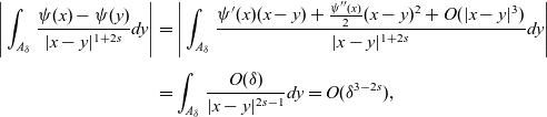 \begin{align*}\Bigg|\int_{A_\delta}\frac{\psi(x)-\psi(y)}{|x-y|^{1+2s}}dy\Bigg|&=\Bigg|\int_{A_\delta}\frac{\psi'(x)(x-y)+\frac{\psi''(x)}{2}(x-y)^2+O(|x-y|^3)}{|x-y|^{1+2s}}dy\Bigg|\\[5pt] & = \int_{A_\delta}\frac{O(\delta)}{|x-y|^{2s-1}}dy=O(\delta^{3-2s}), \end{align*}
and
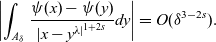 \begin{equation*} \left|\int_{A_{\delta}}\frac{\psi(x)-\psi(y)}{|x-y^{\lambda|^{1+2s}}}dy\right|=O(\delta^{3-2s}). \end{equation*}
Together with the fact that $\psi(y)$
is uniformly bounded, we derive that if R is sufficiently large then
$\psi(y)$
is uniformly bounded, we derive that if R is sufficiently large then
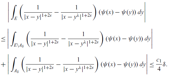 \begin{align}&\Bigg|\int_{E}\left(\frac{1}{|x-y|^{1+2s}}-\frac{1}{|x-y^\lambda|^{1+2s}}\right)\left(\psi(x)-\psi(y)\right)dy\Bigg| \nonumber \\[5pt]&\leq \Bigg|\int_{E\setminus A_\delta}\left(\frac{1}{|x-y|^{1+2s}}-\frac{1}{|x-y^\lambda|^{1+2s}}\right)\left(\psi(x)-\psi(y)\right)dy\Bigg|\\[5pt]&+\Bigg|\int_{A_\delta}\left(\frac{1}{|x-y|^{1+2s}}-\frac{1}{|x-y^\lambda|^{1+2s}}\right)\left(\psi(x)-\psi(y)\right)dy\Bigg|\leq \frac{c_1}{4}\delta.\nonumber \end{align}
(iv). For $y\in \Omega_{R,\eta}$
, we are able to choose large enough R, such that
$y\in \Omega_{R,\eta}$
, we are able to choose large enough R, such that $\psi(x)-\psi(y)\leq 0$
for
$\psi(x)-\psi(y)\leq 0$
for $\Omega_{R,\eta}$
. It is possible since
$\Omega_{R,\eta}$
. It is possible since $\psi(y)$
is bounded away from 0 and
$\psi(y)$
is bounded away from 0 and $\psi(x)\to 0$
as
$\psi(x)\to 0$
as $\delta\to 0$
. It follows that
$\delta\to 0$
. It follows that
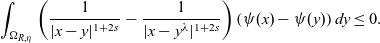 \begin{equation}\begin{aligned}\int_{\Omega_{R,\eta}}\left(\frac{1}{|x-y|^{1+2s}}-\frac{1}{|x-y^\lambda|^{1+2s}}\right)\left(\psi(x)-\psi(y)\right)dy\leq 0.\end{aligned}\end{equation}
Combining (4.18), (4.19), (4.20) and (4.21), we arrive at an estimate on $I_1$
:
$I_1$
:
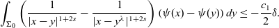 \begin{equation}\int_{\Sigma_0}\left(\frac{1}{|x-y|^{1+2s}}-\frac{1}{|x-y^\lambda|^{1+2s}}\right)\left(\psi(x)-\psi(y)\right)dy\leq-\frac{c_1}{2}\delta.\end{equation}
To estimate $I_2$
, by direct computation, we have
$I_2$
, by direct computation, we have
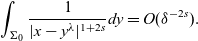 \begin{equation*}\int_{\Sigma_0}\frac{1}{|x-y^\lambda|^{1+2s}}dy=O(\delta^{-2s}).\end{equation*}
Consequently, noticing that the first and second derivatives of $\psi$
vanish at 0, we deduce that
$\psi$
vanish at 0, we deduce that
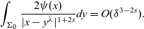 \begin{equation}\int_{\Sigma_0}\frac{2\psi(x)}{|x-y^\lambda|^{1+2s}}dy=O(\delta^{3-2s}).\end{equation}
Finally, since $\psi(y)$
is uniformly bounded at infinity, for l large enough we obtain that
$\psi(y)$
is uniformly bounded at infinity, for l large enough we obtain that
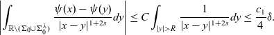 \begin{equation}\left|\int_{\mathbb{R}\setminus(\Sigma_0\cup\Sigma_0^\lambda)}\frac{\psi(x)-\psi(y)}{|x-y|^{1+2s}}dy\right|\leq C\int_{|y|>R}\frac{1}{|x-y|^{1+2s}}dy\leq \frac{c_1}{4}\delta.\end{equation}
On the other hand, we have
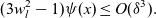 \begin{equation}(3w_l^2-1)\psi(x)\leq O(\delta^3).\end{equation}
Combining (4.22), (4.23), (4.24) and (4.25), we arrive at
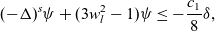 \begin{equation*}(-\Delta)^s\psi+(3w_l^2-1)\psi\leq -\frac{c_1}{8}\delta,\end{equation*}
for sufficiently small $\delta$
, which contradicts to equation (4.16). Thus, we must have
$\delta$
, which contradicts to equation (4.16). Thus, we must have $\psi'(0)<0$
.
$\psi'(0)<0$
.
2. Single (large)-spike solution of Type II. Let $(A(x),B(x))=(A^+,B^+)$
be the single (large)-spike solution of Type II. It is easy to see that
$(A(x),B(x))=(A^+,B^+)$
be the single (large)-spike solution of Type II. It is easy to see that
 \begin{equation}\begin{aligned}-\mu_{L,e}=\min\limits_{\phi\in H^s(\tilde{I}),\int_{\tilde{I}}\phi^2dx=1}a^{1-\frac{1}{2s}}\left[\int_{\hat{I}}\left(|(-\Delta)^{\frac{s}{2}}\phi|^2+\phi^2-3H_l^2\phi^2\right)dy+\beta_L\!\left(\int_{\hat{I}}H_l\phi dy\right)^2\right],\end{aligned}\end{equation}
where
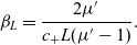 \begin{equation*}\beta_L=\frac{2\mu{'}}{c_+L(\mu{'}-1)}.\end{equation*}
Observing that
 \begin{equation*}\begin{aligned}\lim\limits_{L\to+\infty}\beta_L=\lim\limits_{L\to+\infty}\frac{2\mu{'}}{c_+L(\mu{'}-1)}=\lim\limits_{L\to+\infty}\frac{4\beta_L^1}{c_+\mathrm{I}_{w_\infty}}<\frac{4s}{(2s-1)\mathrm{I}_{w_\infty}},\end{aligned}\end{equation*}
where $\beta_L^1$
is defined in (3.7) and we have used
$\beta_L^1$
is defined in (3.7) and we have used
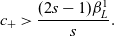 \begin{equation*}c_+>\frac{(2s-1)\beta_L^1}{s}.\end{equation*}
By Theorem 4.1, for $0<\beta<\frac{4s}{(2s-1)\mathrm{I}_{w_\infty}}$
, there exists a unique principal eigenvalue
$0<\beta<\frac{4s}{(2s-1)\mathrm{I}_{w_\infty}}$
, there exists a unique principal eigenvalue $\lambda_0>0$
and a corresponding eigenfunction
$\lambda_0>0$
and a corresponding eigenfunction $\phi_0(y)\in\mathcal{X}_\infty$
satisfying the following eigenvalue problem:
$\phi_0(y)\in\mathcal{X}_\infty$
satisfying the following eigenvalue problem:
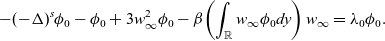 \begin{equation*}-(-\Delta)^s\phi_0-\phi_0+3w_\infty^2\phi_0-\beta\!\left(\int_{\mathbb{R}}w_\infty\phi_0dy\right)w_\infty=\lambda_0\phi_0.\end{equation*}
It is known that $\phi_0(y)=O\!\left(\frac{1}{l^{1+2s}}\right)$
for
$\phi_0(y)=O\!\left(\frac{1}{l^{1+2s}}\right)$
for $|y|\geq l$
, and so by a simple computation we can show that
$|y|\geq l$
, and so by a simple computation we can show that $\phi_0(c_+x)$
makes (4.26) negative.
$\phi_0(c_+x)$
makes (4.26) negative.
3. Double-spike layer solutions of Type III. By Lemma 4.1, the eigenvalue problem:
 \begin{equation*}-(-\Delta)^s\phi_0-\phi_0+3w_\infty^2\phi_0=\lambda_0\phi_0,\quad \phi_0\in H^2(\mathbb{R})\end{equation*}
has an eigenvalue $\lambda_0>0$
with a corresponding eigenfunction
$\lambda_0>0$
with a corresponding eigenfunction $\phi_0$
.
$\phi_0$
.
We now set
 \begin{equation*}\phi(x)=\phi_0\!\left(a^{\frac{1}{2s}}\left(x+\frac{L}{2}\right)\right)+\phi_0\!\left(a^{\frac{1}{2s}}\left(x-\frac{L}{2}\right)\right)+\phi_0(a^{\frac{1}{2s}}x),\quad x\in I.\end{equation*}
Then, we calculate
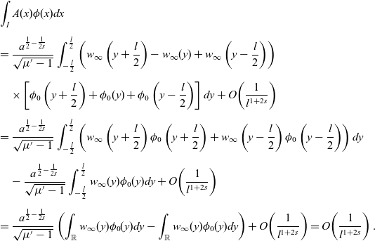 \begin{equation*}\begin{aligned}&\int_{I}A(x)\phi(x)dx\\[5pt]&=\frac{a^{\frac{1}{2}-\frac{1}{2s}}}{\sqrt{\mu{'}-1}}\int_{-\frac{l}{2}}^{\frac{l}{2}}\left(w_\infty\left(y+\frac{l}{2}\right)-w_\infty(y)+w_\infty\left(y-\frac{l}{2}\right)\right)\\[5pt]&\quad \times \left[\phi_0\left(y+\frac{l}{2}\right)+\phi_0(y)+\phi_0\left(y-\frac{l}{2}\right)\right]dy +O\!\left(\frac{1}{l^{1+2s}}\right)\\[5pt]&=\frac{a^{\frac{1}{2}-\frac{1}{2s}}}{\sqrt{\mu{'}-1}}\int_{-\frac{l}{2}}^{\frac{l}{2}}\left(w_\infty\left(y+\frac{l}{2}\right)\phi_0\left(y+\frac{l}{2}\right)+w_\infty\left(y-\frac{l}{2}\right)\phi_0\left(y-\frac{l}{2}\right)\right)dy\\[5pt]&\quad-\frac{a^{\frac{1}{2}-\frac{1}{2s}}}{\sqrt{\mu{'}-1}}\int_{-\frac{l}{2}}^{\frac{l}{2}}w_\infty(y)\phi_0(y)dy+O\!\left(\frac{1}{l^{1+2s}}\right)\\[5pt]&=\frac{a^{\frac{1}{2}-\frac{1}{2s}}}{\sqrt{\mu{'}-1}}\left(\int_{\mathbb{R}}w_\infty(y)\phi_0(y)dy-\int_{\mathbb{R}}w_\infty(y)\phi_0(y)dy\right)+O\!\left(\frac{1}{l^{1+2s}}\right)=O\!\left(\frac{1}{l^{1+2s}}\right).\end{aligned}\end{equation*}
Therefore,
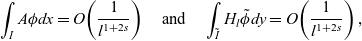 \begin{equation*}\int_{I}A\phi dx=O\!\left(\frac{1}{l^{1+2s}}\right)\quad\textrm{and}\quad\int_{\tilde{I}}H_l\tilde{\phi}dy=O\!\left(\frac{1}{l^{1+2s}}\right),\end{equation*}
where $\tilde\phi(y)=\phi(x),\;y=a^{\frac{1}{2s}}x$
. Hence,
$\tilde\phi(y)=\phi(x),\;y=a^{\frac{1}{2s}}x$
. Hence,
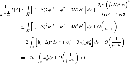 \begin{equation*}\begin{aligned}\frac{1}{a^{1-\frac{1}{2s}}}L[\phi]&\leq \int_{\tilde{I}}\left[|(-\Delta)^{\frac{s}{2}}\tilde{\phi}|^2+\tilde{\phi}^2-3H_l^2\tilde{\phi}^2\right]dy+\frac{2\mu{'}\left(\int_{\tilde{I}}H_l\tilde{\phi}dy\right)^2}{L(\mu{'}-1)a^{\frac{1}{2s}}}\\[5pt]&\leq\int_{\tilde{I}}\left[|(-\Delta)^{\frac{s}{2}}\tilde{\phi}|^2+\tilde{\phi}^2-3H_l^2\tilde{\phi}^2\right]dy+O\!\left(\frac{1}{l^{2+4s}}\right)\\[5pt]&=2\int_{\mathbb{R}}\left[|(-\Delta)^{\frac{s}{2}}\phi_0|^2+\phi_0^2-3w_\infty^2\phi_0^2\right]dy+O\!\left(\frac{1}{l^{1+2s}}\right)\\[5pt]&=-2\nu_1\int_{\mathbb{R}}\phi_0^2dy+O\!\left(\frac{1}{l^{1+2s}}\right)<0.\end{aligned}\end{equation*}
Therefore, we have $\mu_{L,e}>0$
, and it shows that the double-spike solution of Type III is unstable. At this point, we have completed the whole proof of Theorem 1.2.
$\mu_{L,e}>0$
, and it shows that the double-spike solution of Type III is unstable. At this point, we have completed the whole proof of Theorem 1.2.
5 Numerical computations
We present the results of numerical computations for the shapes of the single-spike solutions for $s=0.60,\,0.75,\,0.90,\,0.99$
. We implemented two different numerical schemes in Matlab. Both are based on parabolic problems such that the stable steady-state solutions are obtained as long-time limits. The numerical schemes use finite difference methods, in particular, a combination of the methods of Crank–Nicolson [Reference Crank and Nicolson6] and Adams–Bashforth.
$s=0.60,\,0.75,\,0.90,\,0.99$
. We implemented two different numerical schemes in Matlab. Both are based on parabolic problems such that the stable steady-state solutions are obtained as long-time limits. The numerical schemes use finite difference methods, in particular, a combination of the methods of Crank–Nicolson [Reference Crank and Nicolson6] and Adams–Bashforth.
Scheme 1. To compute the shape of the single-spike solutions, we implemented a code for the first equation of (1.2) using the Crank–Nicolson method for the linear terms and the Adams–Bashforth method for the non-linear terms. We consider the problem in the spatial interval $\Omega=(-20\pi,20\pi)$
. We substitute
$\Omega=(-20\pi,20\pi)$
. We substitute $B(x)=-\mu{'}(A^2)(x)+\mu{'}\int_\Omega A^2\,dx/|\Omega$
into the first equation and solve it with periodic boundary conditions. For the parameter values, we take
$B(x)=-\mu{'}(A^2)(x)+\mu{'}\int_\Omega A^2\,dx/|\Omega$
into the first equation and solve it with periodic boundary conditions. For the parameter values, we take $0.1^{2s}$
as the diffusion constant of
$0.1^{2s}$
as the diffusion constant of $-(-\Delta)^s A$
and
$-(-\Delta)^s A$
and $\mu{'}=1.001$
. We take into account
$\mu{'}=1.001$
. We take into account $2^{10}$
Fourier modes. The time step is 0.01.
$2^{10}$
Fourier modes. The time step is 0.01.
Scheme 2. To verify that the steady-state solutions computed by Scheme are also long-time limits of the full system (1.2), we implemented a code for the full system (1.2). For the first equation, we used the Crank–Nicolson method for the linear terms and the Adams–Bashforth method for the non-linear terms, in the same way as for Scheme . For the second equation, we used the same discretisation method for both fractional Laplacians so that the numerical scheme satisfies the conservation law exactly which lead us to choosing the forward Euler method. We took a small value for $\tau$
, namely
$\tau$
, namely $\tau=0.1$
. The other parameters are the same as in Scheme . Again, we take into account
$\tau=0.1$
. The other parameters are the same as in Scheme . Again, we take into account $2^{10}$
Fourier modes. The time step has to be taken smaller than in Scheme in order to avoid numerical instability. We chose 0.001 for
$2^{10}$
Fourier modes. The time step has to be taken smaller than in Scheme in order to avoid numerical instability. We chose 0.001 for $s=0.60,\,0.75$
, 0.0005 for
$s=0.60,\,0.75$
, 0.0005 for $s=0.90$
and 0.0003 for
$s=0.90$
and 0.0003 for $s=0.99$
.
$s=0.99$
.
We have chosen as initial values $A(x)=\frac{2}{1+x^2}$
and
$A(x)=\frac{2}{1+x^2}$
and $B(x)=0$
.
$B(x)=0$
.
The following figure shows the shapes of the spikes obtained by using Scheme based on the reduced system for the first equation of (1.2). These shapes have been confirmed as long-time limits of the full system by using Scheme . Numerically, in both schemes, the solutions converge to the same spike profile. Since the shapes for Scheme are indistinguishable from those of Scheme , they have not been included.
We observe from Figure 1 that for increasing values of s the spikes become narrower and their spatial decay becomes faster, in agreement with Theorem 1.1.

Figure 1. Spiky steady states of (1.2) for $\mu{'}=1.001,\,\tau=0.1$
achieved as long-time limits of Scheme with initial conditions
$\mu{'}=1.001,\,\tau=0.1$
achieved as long-time limits of Scheme with initial conditions $A(x)=\frac{2}{1+x^2}$
and
$A(x)=\frac{2}{1+x^2}$
and $B(x)=0.$
Spiky steady states for (1.2) have been presented for the parameter values
$B(x)=0.$
Spiky steady states for (1.2) have been presented for the parameter values $s=0.60,\,0.75,\,0.90,\,0.99$
. We have shown A(x) on the left and B(x) on the right, both restricted to the interval
$s=0.60,\,0.75,\,0.90,\,0.99$
. We have shown A(x) on the left and B(x) on the right, both restricted to the interval $-10<x<10$
. The maximum values of the spike pattern A(x) increases with s, and we have computed the maximum values as
$-10<x<10$
. The maximum values of the spike pattern A(x) increases with s, and we have computed the maximum values as $3.52,\,10.73,\,14.31,\,15.68$
.
$3.52,\,10.73,\,14.31,\,15.68$
.
For $s=0.51$
in both schemes, the solutions converge to the homogeneous steady state
$s=0.51$
in both schemes, the solutions converge to the homogeneous steady state $A=1$
,
$A=1$
, $B=0$
. Scheme gives an error of the order
$B=0$
. Scheme gives an error of the order $10^{-3}$
due to the use of the trapezoidal rule for integration. Scheme does not use any numerical integration, and the error is of the order
$10^{-3}$
due to the use of the trapezoidal rule for integration. Scheme does not use any numerical integration, and the error is of the order $10^{-10}$
.
$10^{-10}$
.
We further investigated the threshold value of s for which the solution converges to a spike solution or the homogeneous steady state $A=1,\,B=1$
. Using both Scheme and Scheme , we found that for
$A=1,\,B=1$
. Using both Scheme and Scheme , we found that for $s=0.58$
or below we get a homogeneous steady state but for
$s=0.58$
or below we get a homogeneous steady state but for $s=0.59$
or above a spike solution is formed. The computations have to be done carefully near the threshold, since the solution can stay for a long time in a state which looks like a spike solution before it either contracts to a homogeneous steady state or approaches an exact spike solution. This threshold is in qualitative agreement with the theoretical result in (1.8). Since the value of
$s=0.59$
or above a spike solution is formed. The computations have to be done carefully near the threshold, since the solution can stay for a long time in a state which looks like a spike solution before it either contracts to a homogeneous steady state or approaches an exact spike solution. This threshold is in qualitative agreement with the theoretical result in (1.8). Since the value of $\mathrm{I}_{w_\infty}$
is unknown, further quantitative comparisons are not possible. We leave this as an open problem for future research.
$\mathrm{I}_{w_\infty}$
is unknown, further quantitative comparisons are not possible. We leave this as an open problem for future research.
In summary, we have computed the spike solutions and the homogeneous steady states $A=1,\,B=0$
as long-time limits of the parabolic problem (1.1), using two different numerical schemes for
$A=1,\,B=0$
as long-time limits of the parabolic problem (1.1), using two different numerical schemes for $\mu{'}=1.001$
. For
$\mu{'}=1.001$
. For $s=0.59$
or above, the solutions converge to a spike solution which indicates that the spike solution exists in this parameter range and is stable. For
$s=0.59$
or above, the solutions converge to a spike solution which indicates that the spike solution exists in this parameter range and is stable. For $s=0.58$
or below, the solutions convergence to the homogeneous steady state
$s=0.58$
or below, the solutions convergence to the homogeneous steady state $A=1,\,B=0$
which indicates that in this parameter range the homogeneous steady state is stable. From Theorem 1.1, we know that the spike solution does not exist in this parameter range. We have found qualitative agreement between the theoretical threshold predicted in (1.8) and the numerical results.
$A=1,\,B=0$
which indicates that in this parameter range the homogeneous steady state is stable. From Theorem 1.1, we know that the spike solution does not exist in this parameter range. We have found qualitative agreement between the theoretical threshold predicted in (1.8) and the numerical results.
The threshold (1.8) is a typical feature of the Ginzburg–Landau equation with a mean field, and it is ultimately a consequence of the consistency condition (2.2). We also found that by using consistency condition (2.2), the numerical computations can be simplified substantially and included (2.2) in Scheme .
6 Conclusion
We summarize the results of this paper, draw some conclusions and give an outlook.
We have considered the existence and stability of three types of singular patterns in a fractional Ginzburg–Landau system with a mean field which has been derived from a fractional fluid mechanics model with symmetry-breaking term.
The expansion for the amplitude equations given in (1.4) and (1.5) uses an interesting scaling. In particular, the scaling of time has a fractional order of the small parameter $\varepsilon$
which comes from the fractional Laplacian. However, the scaling of space does not have a fractional order of the small parameter. Alternatively, scalings can be chosen which have the small parameters distributed between the temporal and spatial terms. We remark that it is possible to define a new small parameter:
$\varepsilon$
which comes from the fractional Laplacian. However, the scaling of space does not have a fractional order of the small parameter. Alternatively, scalings can be chosen which have the small parameters distributed between the temporal and spatial terms. We remark that it is possible to define a new small parameter: $\tilde{\varepsilon}=\varepsilon^{2s}$
, whereby the fractional scaling will move from t to x. It is also possible to split it:
$\tilde{\varepsilon}=\varepsilon^{2s}$
, whereby the fractional scaling will move from t to x. It is also possible to split it: $T = \tilde{\varepsilon}^{2s}t$
and
$T = \tilde{\varepsilon}^{2s}t$
and $X =\tilde{\varepsilon}^{1/\sqrt{2s}}x$
. Any arbitrary split such that
$X =\tilde{\varepsilon}^{1/\sqrt{2s}}x$
. Any arbitrary split such that $\varepsilon_x^{2s}=\varepsilon_t$
would work.
$\varepsilon_x^{2s}=\varepsilon_t$
would work.
There are a lot of studies on the derivation of amplitude equations for fractional-order partial derivatives in the recent decades, see [Reference Milovanov and Juul Rasmussen14, Reference Nec, Nepomnyashchy and Golovin17, Reference Tarasov and Zaslavsky25] for instance. We expect the results of the current article could provide some new insights to stimulate the development of this direction in the future.
The periodic patterns investigated are the most basic ones, namely double fronts, single spikes and double spikes. It is an important question to understand which of these patterns is preferred by the model equations and will persist in the dynamical behaviour. This motivates the study of stable vs. unstable solutions. It turns out that one of the single-spike solutions is stable, whereas the other solutions are all unstable. We can conclude that in this model spiky patterns are preferred over front patterns.
The methods used in this paper are extensions of [Reference Norbury, Wei and Winter19]. We find it interesting that it was possible to generalise the approach in [Reference Norbury, Wei and Winter19] to the fractional Laplacian setting. Although many qualitative properties remain the same, we have observed that the asymptotic behaviour for increasing spatial period changes throughout the analysis.
It will be interesting to extend the results of this study from one space dimension to several spatial dimensions. Another possible direction for future work is the investigation of pattern formation in systems of PDEs with different types of fractional terms.
Acknowledgement
The research of the third author is supported by NSFC Grants 11871470, 12171456 and 12271369. We thank the referee very much for many excellent suggestions which helped us to improve the paper.
Conflict of interests
None.


 Open access